1  

Estimating Acoustic Performance of a Cell Phone Speaker Using Abaqus

C. Jackman1, M. Zampino1

D. Cadge2, R. Dravida2, V. Katiyar2, J. Lewis2

1Foxconn Holdings LLC

2DS SIMULIA

Abstract: Consumers demand smaller electronics devices with more features and capabilities. Making devices smaller provides challenges to engineers to maintain the acoustic performances as enclosed acoustic volume sizes are reduced. This paper discusses the requirements for coupled structural-acoustic simulation and demonstrates the application of this technology to cell-phone acoustic design. Due to the smaller volume sizes, the low frequency response of the cell phone is affected. The frequency response rolls off faster at low frequencies when smaller microphone back volumes are used. The present work deals with studying this effect on a simple cell phone model with the finite element package, Abaqus. The results from the simulation can be used in better designing cell phone cavities for optimum performance.

Keywords: Diaphragm, Acoustics, Impedance Boundary, Topology, Merge/Cut, Tie, Back Volume

1. Introduction

Cell phone industry has been making great advances in terms of packing more features while reducing the size of the instrument itself. As the size reduces, it presents more challenges to the overall acoustic performance of the cell phone. At low frequencies, the acoustic pressure emitted by a cell phone device is affected by the size of the back volume which in turn is affected by the size of the instrument. Hence, in order to improve the acoustic performance cell phone designers often use more than one speaker. Additionally, the size of the back volume that would give the optimum acoustic performance has to be prototyped and developed. Fortunately the availability of finite element software codes, such as Abaqus, avoids the time consuming and expensive process of building and rebuilding of back volumes to physically test the optimum performance.

2  

Abaqus’s general nonlinear mechanics capabilities have been used for twist, hyperextension and drop test simulations (Nagaraj, 2002; Thiruppukuzhi, 2008; Theman, 2005). The general mechanics capabilities clubbed with the coupled structural-acoustic capabilities make Abaqus a powerful tool to solve the most important problems related to the cell phone industry. Powerful Abaqus/CAE modeling capabilities (including easy import of geometry from third party CAD software, a wide variety of meshing tools, virtual topology etc) along with a number of structural, acoustic element types and a broad range of material models make Abaqus a versatile software for these kinds of simulations. Additional features include nonconforming tie between structural and acoustic elements, and availability of a variety of acoustic output variables. In the present work, we setup a dual-speaker model in Abaqus and compare the simulation results of the acoustic pressure at a certain distance in the exterior of the diaphragm when the speakers are excited by a mechanical force.

2. Physics of the problem

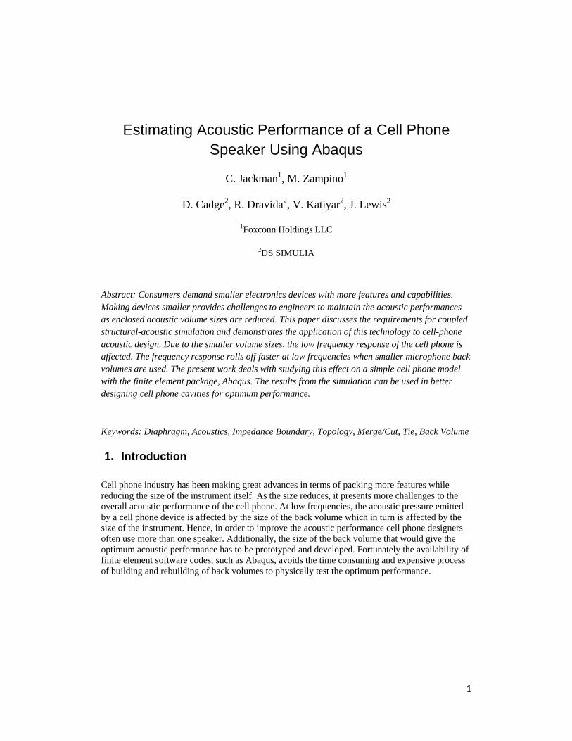
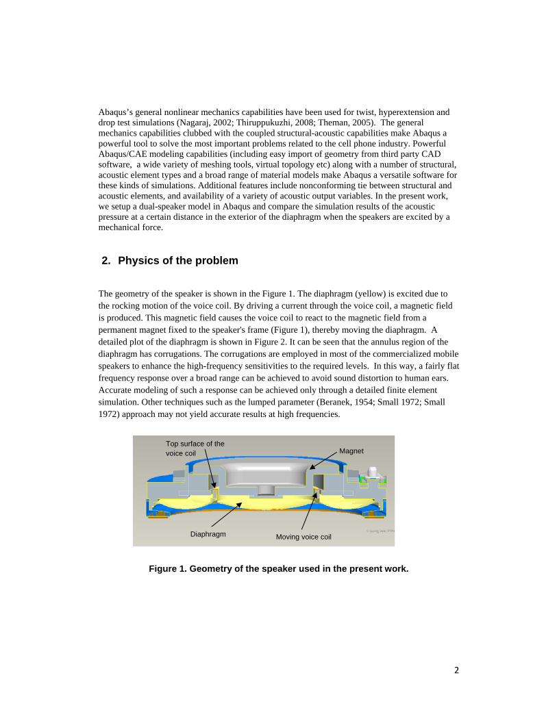
The geometry of the speaker is shown in the Figure 1. The diaphragm (yellow) is excited due to the rocking motion of the voice coil. By driving a current through the voice coil, a magnetic field is produced. This magnetic field causes the voice coil to react to the magnetic field from a permanent magnet fixed to the speaker's frame (Figure 1), thereby moving the diaphragm. A detailed plot of the diaphragm is shown in Figure 2. It can be seen that the annulus region of the diaphragm has corrugations. The corrugations are employed in most of the commercialized mobile speakers to enhance the high-frequency sensitivities to the required levels. In this way, a fairly flat frequency response over a broad range can be achieved to avoid sound distortion to human ears. Accurate modeling of such a response can be achieved only through a detailed finite element simulation. Other techniques such as the lumped parameter (Beranek, 1954; Small 1972; Small 1972) approach may not yield accurate results at high frequencies.

Figure 1. Geometry of the speaker used in the present work.

Diaphragm

Magnet

Moving voice coil

Top surface of the voice coil

3  

As the size of the cell phone decreases, the volume of air behind the diaphragm becomes smaller. This small amount of volume behind the speaker limits the range of motion of the diaphragm. The speaker does not produce enough force to compress the air beyond a certain point, hence causing the air to push back. This reduces the displacement of the speaker diaphragm, which in turn lowers the output. The frequencies affected the most by this are the ones with the largest amount of displacement, (low frequencies). This effect can be modeled in Abaqus using acoustic elements, which have predefined bulk properties to capture such volumetric effects automatically.

Figure 2. Diaphragm.

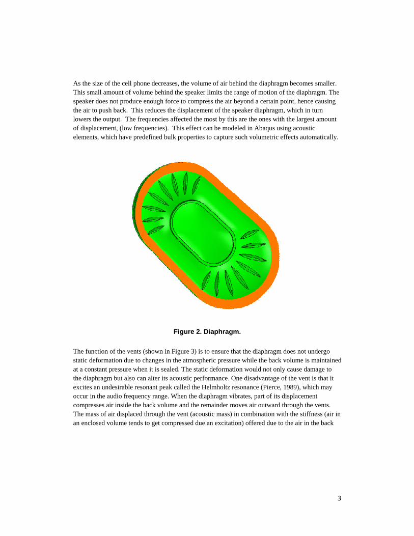
The function of the vents (shown in Figure 3) is to ensure that the diaphragm does not undergo static deformation due to changes in the atmospheric pressure while the back volume is maintained at a constant pressure when it is sealed. The static deformation would not only cause damage to the diaphragm but also can alter its acoustic performance. One disadvantage of the vent is that it excites an undesirable resonant peak called the Helmholtz resonance (Pierce, 1989), which may occur in the audio frequency range. When the diaphragm vibrates, part of its displacement compresses air inside the back volume and the remainder moves air outward through the vents. The mass of air displaced through the vent (acoustic mass) in combination with the stiffness (air in an enclosed volume tends to get compressed due an excitation) offered due to the air in the back

4  

volume produces the Helmholtz resonance. In order to tune this peak to acceptable levels, the speaker manufacturers apply a netted material on the vent.

Figure 3. Bottom view of the speaker geometry showing the vents. 3. Model Setup

We have taken two approaches to run the simulations. One is to replace the convoluted membrane with a planar membrane and tune the material properties (Young’s modulus and density) and thickness of the membrane materials. The method relies on experimental data for two cases; case 1, when the speaker’s back volume is enclosed such that the volume of air contained in it is 2cc and case 2, when the speaker’s front and back volumes are separated such that there is no acoustic interaction between them (this condition is referred to as an infinite baffle in the literature). The thickness and density of the voice coil and the diaphragm are tuned such that the simulation results match the experimental results of both cases. The results obtained by

Vents

5  

performing simulations with the tuned parameters have to be compared with another measurement with a different back volume. This is a work in progress as we will be comparing the tuned results with a 3.5 cc back volume case.

The second approach is to model the actual dual-speaker geometry in Abaqus. This methodology is advantageous because the physics of the problem is captured accurately without the need for any approximations. Also since we are using the actual geometry and the material properties, the laborious tuning methodology employed in the first approach can be completely avoided.

The original CAD speaker model was imported into Abaqus/CAE. Abaqus/CAE is a CAD neutral system, and is designed to be able to import and use geometry from many third party proprietary CAD systems, as well as neutral file formats. In some cases parts or part instances contain details such as very small faces and edges. These features, although important for machining and packaging of a component, have little impact on the mechanics of the problem. Including such features in the numerical analysis may lead to very fine mesh density leading to increased computation times. The virtual topology feature in Abaqus/CAE allowed us to exclude such small details by combining the feature with an adjacent larger feature. Nodes and elements are still created to conform to the original geometry.

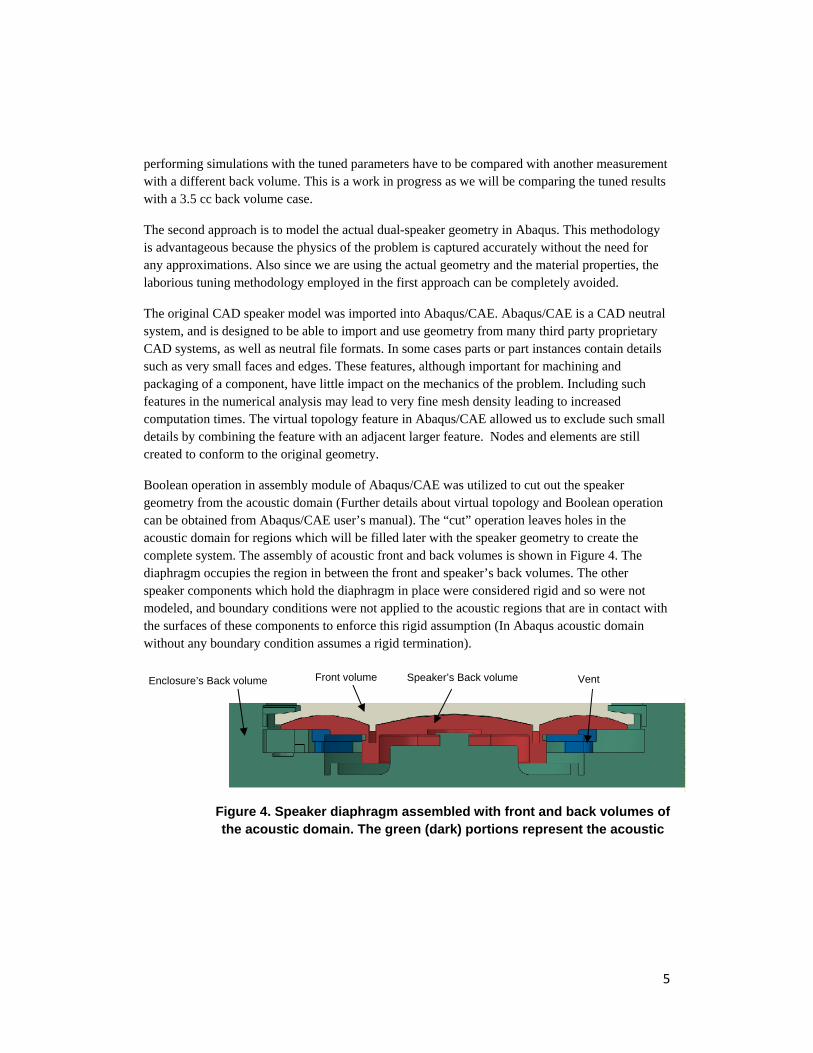
Boolean operation in assembly module of Abaqus/CAE was utilized to cut out the speaker geometry from the acoustic domain (Further details about virtual topology and Boolean operation can be obtained from Abaqus/CAE user’s manual). The “cut” operation leaves holes in the acoustic domain for regions which will be filled later with the speaker geometry to create the complete system. The assembly of acoustic front and back volumes is shown in Figure 4. The diaphragm occupies the region in between the front and speaker’s back volumes. The other speaker components which hold the diaphragm in place were considered rigid and so were not modeled, and boundary conditions were not applied to the acoustic regions that are in contact with the surfaces of these components to enforce this rigid assumption (In Abaqus acoustic domain without any boundary condition assumes a rigid termination).

Figure 4. Speaker diaphragm assembled with front and back volumes of the acoustic domain. The green (dark) portions represent the acoustic

Enclosure’s Back volume Front volume Speaker’s Back volume Vent

6  

domain. Grey (light) portion represents the diaphragm and the moving coil. The void region represents the rigid components of the speaker.

3.1 Elements, Boundary Conditions, Loads and Domain Size:

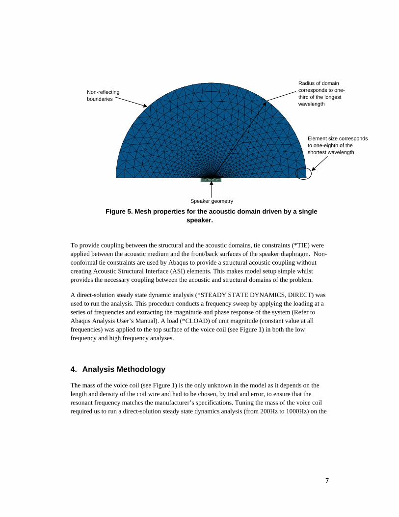
The diaphragm is modeled with modified three-dimensional solid elements (Abaqus keyword *ELEMENT, TYPE=C3D10M) and was assigned the physical properties for the material of the diaphragm given as per the manufacturer’s specifications. Modeling the diaphragm with solid elements (instead of shell elements) allowed us to cut away the acoustic domain more easily. The acoustic domain, both in the back volume and the volume exterior to the diaphragm, is modeled with three-dimensional acoustic elements (*ELEMENT, TYPE=AC3D4). These elements were assigned the physical properties of air. For problems that include unbounded acoustic domain, a boundary condition has to be applied at the exterior boundary to minimize reflections. This can be achieved by applying nonreflecting surface impedance boundary conditions (*SIMPEDANCE, TYPE=SPHERICAL) to the exterior mesh as shown in Figure 5. A pinned boundary condition was applied on the outer surface of the diaphragm (red or dark region in Figure 2) which in the actual speaker geometry was sandwiched between two bodies.

The accuracy of an acoustic analysis depends on two factors: element size in the acoustic domain and the overall size of the exterior domain. It is recommended that at least six representative inter nodal intervals fit into the shortest wavelength present in the analysis. Generally, if greater accuracy is desired 8 to 10 elements per wavelength should be used. If the domain size is many wavelengths at least 15 elements per wavelength have to be used to counter numerical dispersion. The numerical dispersion is the decay in acoustic pressure as a function of distance solely due to accumulation of numerical errors from one element to the next, which is a result of having fewer elements per wavelength (Figure 5 has an illustration of finite element mesh considerations for an acoustic analysis). In the present work, eight elements per wavelength were chosen to run the analysis. It is recommended that the domain size is at least 1/3rd of the longest wavelength (lowest frequency present in the analysis). This number, although arbitrary, ensures that the reflections from the far field are minimized when the acoustic boundary is terminated with nonreflecting impedance boundary conditions.

As the frequency range of interest grows the size of the model may approach the upper limit of memory and disk space on the computer. Hence, it is advisable to split the analysis into multiple runs with smaller frequency ranges of interest. In the present analysis our frequency range of interest from 200 Hz to 5000 Hz is split into two analyses; one from 200 Hz to 1000 Hz (Low frequency analysis) and the other from 1000 Hz to 5000 Hz (High frequency analysis).

7  

Figure 5. Mesh properties for the acoustic domain driven by a single speaker.

To provide coupling between the structural and the acoustic domains, tie constraints (*TIE) were applied between the acoustic medium and the front/back surfaces of the speaker diaphragm. Non-conformal tie constraints are used by Abaqus to provide a structural acoustic coupling without creating Acoustic Structural Interface (ASI) elements. This makes model setup simple whilst provides the necessary coupling between the acoustic and structural domains of the problem.

A direct-solution steady state dynamic analysis (*STEADY STATE DYNAMICS, DIRECT) was used to run the analysis. This procedure conducts a frequency sweep by applying the loading at a series of frequencies and extracting the magnitude and phase response of the system (Refer to Abaqus Analysis User’s Manual). A load (*CLOAD) of unit magnitude (constant value at all frequencies) was applied to the top surface of the voice coil (see Figure 1) in both the low frequency and high frequency analyses.

4. Analysis Methodology

The mass of the voice coil (see Figure 1) is the only unknown in the model as it depends on the length and density of the coil wire and had to be chosen, by trial and error, to ensure that the resonant frequency matches the manufacturer’s specifications. Tuning the mass of the voice coil required us to run a direct-solution steady state dynamics analysis (from 200Hz to 1000Hz) on the

Speaker geometry

Radius of domain corresponds to one-third of the longest wavelength

Element size corresponds to one-eighth of the shortest wavelength

Non-reflecting boundaries

8  

diaphragm, without the acoustic domain, in the presence of high enough damping in order to obtain the displacement response at the center of the diaphragm. The damping of the diaphragm (*STRUCTURAL DAMPING) was chosen such that the quality factor (Pierce, 1989; Thiel, 1972) at the resonant peak matches with the manufacturer’s specification. Additional damping was added to account for the electrical effects. The effect of the magnetic field, length of copper wire used to create the electro-magnet, as well as the resistance of this copper wire, is to create a resistance in series with the structural damping resistance provided by the diaphragm (See paper by Thiel: “Loudspeakers in Vented Boxes: Part-1” Figure 3), and the applied excitation load is scaled independent of frequency. This means that the effect of the electro-magnetic parts of the system is to add damping to the system (Thiel, 1972).

At the end of this process, the actual displacement may not match the experimental measurements but the general shape of the curve will align. This is because of using an approximate unit load as the forcing function. The physical forcing function on the diaphragm cannot be calculated in Abaqus as it is based on electrical excitation (If the electrical circuit is simple enough to be approximated by a lumped parameter model, it may be possible to calculate the equivalent mechanical components and run the complete electro-mechanical analysis in Abaqus. The static characteristics of the electromagnetic driver and its effect on the mechanical displacement of the diaphragm can be obtained by creating a user element) and hence the loading has to be approximated. It is also assumed that the force (as a function of frequency) is independent of the size of the back volume. Since the diaphragm displacement and the subsequent acoustic response are considered to be linear phenomena, the results can be scaled after the analysis to match the measurements. The following paragraph details the scaling procedure.

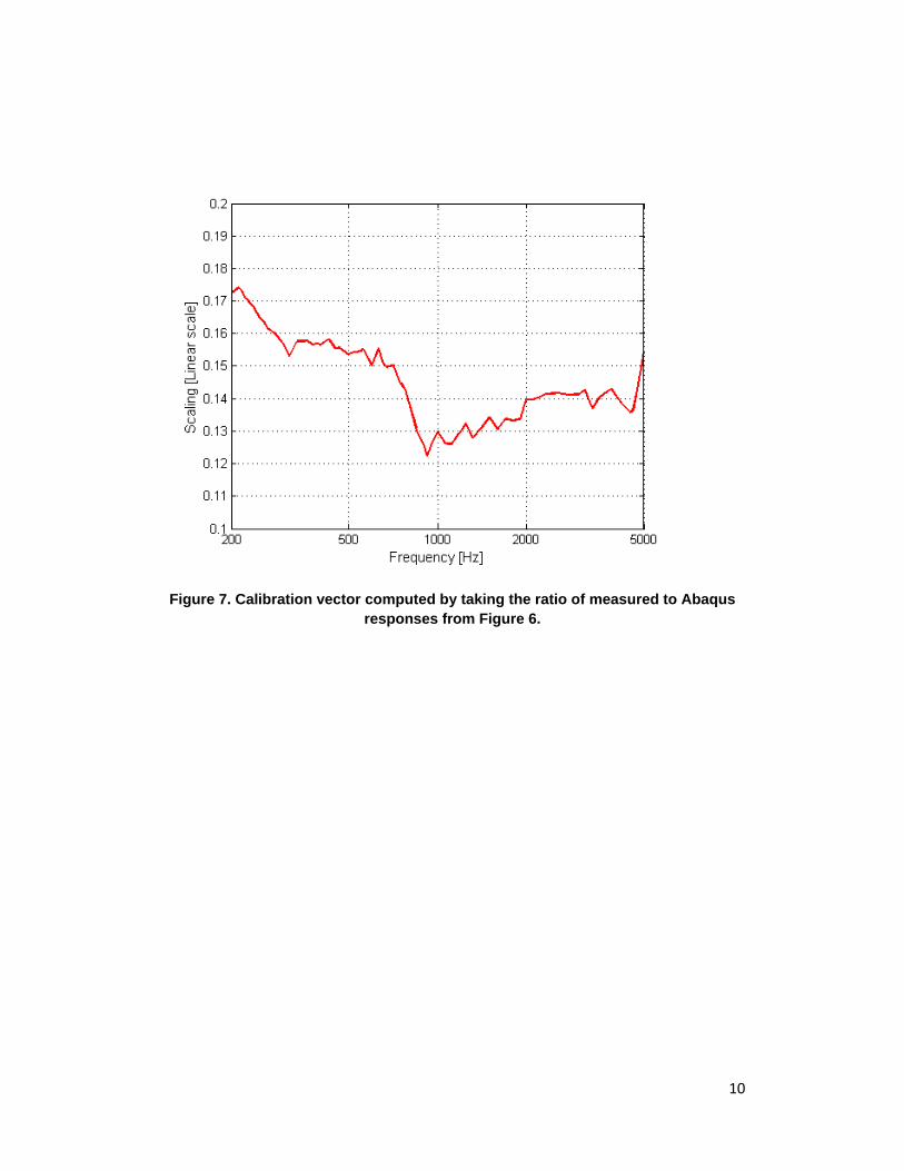
The analysis is performed assuming a unit load on the top surface of the voice coil (see Figure 1) and a calibration vector, which is a linear ratio of the acoustic pressure measured to the acoustic pressure from the Abaqus results as a function of frequency, is calculated. This calibration vector can be multiplied with the acoustic pressure results from subsequent analyses (with different back volumes), provided that unit excitation is applied on the diaphragm in those cases as well.

5. Acoustic pressure and displacement calculations

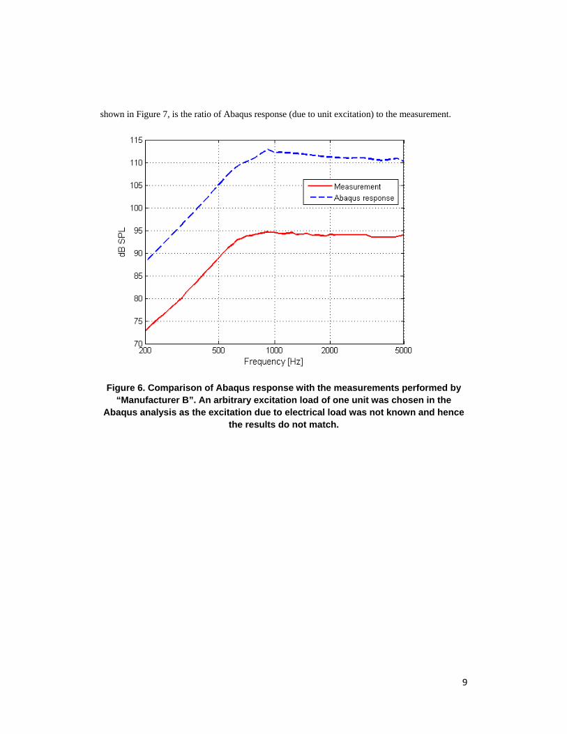
The acoustic pressure in the exterior domain at a distance of 10 cm away is shown in Figure 6. The mechanical force applied on the diaphragm (due to the electrical excitation) was not known and so an arbitrary value of 1 unit load was chosen to run the Abaqus simulation. Hence, the results in Figure 6 do not match but the general shape of the curves is identical. The calibration vector,

9  

shown in Figure 7, is the ratio of Abaqus response (due to unit excitation) to the measurement.

Figure 6. Comparison of Abaqus response with the measurements performed by “Manufacturer B”. An arbitrary excitation load of one unit was chosen in the

Abaqus analysis as the excitation due to electrical load was not known and hence the results do not match.

10  

Figure 7. Calibration vector computed by taking the ratio of measured to Abaqus responses from Figure 6.

11  

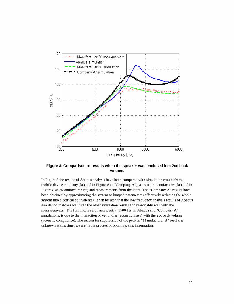
Figure 8. Comparison of results when the speaker was enclosed in a 2cc back volume.

In Figure 8 the results of Abaqus analysis have been compared with simulation results from a mobile device company (labeled in Figure 8 as “Company A”), a speaker manufacturer (labeled in Figure 8 as “Manufacturer B”) and measurements from the latter. The “Company A” results have been obtained by approximating the system as lumped parameters (effectively reducing the whole system into electrical equivalents). It can be seen that the low frequency analysis results of Abaqus simulation matches well with the other simulation results and reasonably well with the measurements. The Helmholtz resonance peak at 1500 Hz, in Abaqus and “Company A” simulations, is due to the interaction of vent holes (acoustic mass) with the 2cc back volume (acoustic compliance). The reason for suppression of the peak in “Manufacturer B” results is unknown at this time; we are in the process of obtaining this information.

12  

6. Conclusions

The present work shows that acoustic analysis in Abaqus can capture a) Helmholtz resonance and b) the reduction in acoustic pressure at low frequencies due to the presence of back volume. These effects play an important role in choosing the appropriate back-volume size during a cell phone design and in choosing the appropriate vent size during the speaker design.

The results of Abaqus simulations have been compared to those from a mobile device company and a speaker manufacturer. The results below 1000 Hz agree very well between the three simulations and the measurement. The Helmholtz resonance peak that exists in Abaqus, “Company A” results is not seen in “Manufacturer B” results and the subsequent higher frequencies are also affected by the resonant peak. The reason for this discrepancy is being investigated.

7. Future work

Several improvements can be made to the modeling strategy to reduce the analysis time.

1. Infinite elements can be employed instead of the nonreflecting impedance boundary conditions. The domain size required for infinite elements to work effectively is much smaller than the size required for nonreflecting boundaries. The infinite element formulation has a ninth-order truncation of the reflections, where as the nonreflecting boundaries have a zero-order approximation.

2. Use mode-based steady state dynamics (*STEADY STATE DYNAMICS, SUBSPACE) instead of the direct solution (*STEADY STATE DYNAMICS, DIRECT).

3. Model the diaphragm with shell elements instead of solid elements. This will reduce additional computation time associated with solving equations of the solid elements.

8. References

1. Beranek, L. L., “Noise and vibration control”, McGraw-Hill, New York, 1954. 2. Nagaraj, B., Motorola, "Two Step Method of Analyzing Hyperextension Problems with

Large Contact Interactions Using Abaqus/Explicit," Abaqus Users' Conference, pp. 1 – 7, Newport, Rhode Island, May 2002.

3. Pierce, A. D., “Acoustics: An Introduction to Physical Principles and Applications”, Acoustical Society of America, pp. 121, 330, 1989.

13  

4. Small, R. H, “Direct-Radiator Loudspeaker System Analysis”, Journal of Audio Engineering Society, Vol. 20, Num. 5, pp. 383-395, June 1972.

5. Small, R. H., “Closed-box loudspeaker systems-part 1: analysis” J Audio Eng Soc, Vol. 20, Num. 10, pp.798–808, 1972.

6. Theman, M., and Poskiparta, P., Nokia, "Evolution of Mobile Phone Drop Test Simulation at Nokia," Abaqus Users' Conference, pp. 1 – 1, Stockholm, Sweden, May 2005.

7. Thiel, A. N, “Loudspeakers in Vented Boxes: Part I”, Journal of Audio Engineering Society, Vol. 19, Num. 5, pp. 382-391, May 1971.

8. Thiel, A. N, “Loudspeakers in Vented Boxes: Part II”, Journal of Audio Engineering Society, Vol. 19, Num. 6, pp. 471-483, June 1971.

9. Thiruppukuzhi, S., Motorola," Probabilistic Simulation Applications in Product Design," Abaqus Users' Conference, pp. 285 – 301, Newport, Rhode Island, May 2008.