Estimates of species extinctions from speciesarea ...€¦ · Estimates of species extinctions from...
12
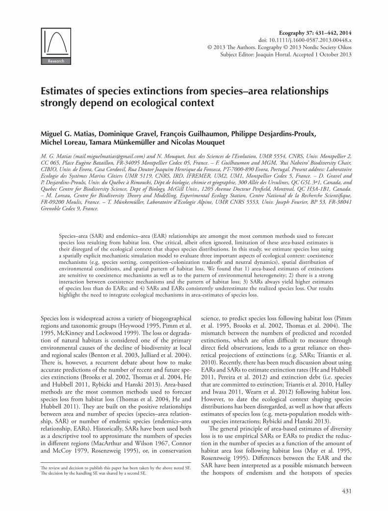
431 Estimates of species extinctions from species–area relationships strongly depend on ecological context Miguel G. Matias, Dominique Gravel, François Guilhaumon, Philippe Desjardins-Proulx, Michel Loreau, Tamara Münkemüller and Nicolas Mouquet M. G. Matias ([email protected]) and N. Mouquet, Inst. des Sciences de l’Evolution, UMR 5554, CNRS, Univ. Montpellier 2, CC 065, Place Eugène Bataillon, FR-34095 Montpellier Cedex 05, France. – F. Guilhaumon and MGM, ‘Rui Nabeiro’ Biodiversity Chair, CIBIO, Univ. de Evora, Casa Cordovil, Rua Doutor Joaquim Henrique da Fonseca, PT-7000-890 Evora, Portugal. Present address: Laboratoire Ecologie des Systèmes Marins Côtiers UMR 5119, CNRS, IRD, IFREMER, UM2, UM1, Montpellier Cedex 5, France. – D. Gravel and P. Desjardins-Proulx, Univ. du Québec à Rimouski, Dépt de biologie, chimie et géographie, 300 Allée des Ursulines, QC G5L 3ª1, Canada, and Quebec Centre for Biodiversity Science, Dept of Biology, McGill Univ., 1205 Avenue Docteur Penfield, Montreal, QC H3A-1B1, Canada. – M. Loreau, Centre for Biodiversity eory and Modelling, Experimental Ecology Station, Centre National de la Recherche Scientifique, FR-09200 Moulis, France. – T. Münkemüller, Laboratoire d’Ecologie Alpine, UMR CNRS 5553, Univ. Joseph Fourier, BP 53, FR-38041 Grenoble Cedex 9, France. Species–area (SAR) and endemics–area (EAR) relationships are amongst the most common methods used to forecast species loss resulting from habitat loss. One critical, albeit often ignored, limitation of these area-based estimates is their disregard of the ecological context that shapes species distributions. In this study, we estimate species loss using a spatially explicit mechanistic simulation model to evaluate three important aspects of ecological context: coexistence mechanisms (e.g. species sorting, competition–colonization tradeoffs and neutral dynamics), spatial distribution of environmental conditions, and spatial pattern of habitat loss. We found that 1) area-based estimates of extinctions are sensitive to coexistence mechanisms as well as to the pattern of environmental heterogeneity; 2) there is a strong interaction between coexistence mechanisms and the pattern of habitat loss; 3) SARs always yield higher estimates of species loss than do EARs; and 4) SARs and EARs consistently underestimate the realized species loss. Our results highlight the need to integrate ecological mechanisms in area-estimates of species loss. Species loss is widespread across a variety of biogeographical regions and taxonomic groups (Heywood 1995, Pimm et al. 1995, McKinney and Lockwood 1999). e loss or degrada- tion of natural habitats is considered one of the primary environmental causes of the decline of biodiversity at local and regional scales (Benton et al. 2003, Julliard et al. 2004). ere is, however, a recurrent debate about how to make accurate predictions of the number of recent and future spe- cies extinctions (Brooks et al. 2002, omas et al. 2004, He and Hubbell 2011, Rybicki and Hanski 2013). Area-based methods are the most common methods used to forecast species loss from habitat loss (omas et al. 2004, He and Hubbell 2011). ey are built on the positive relationships between area and number of species (species–area relation- ship, SAR) or number of endemic species (endemics–area relationship, EARs). Historically, SARs have been used both as a descriptive tool to approximate the numbers of species in different regions (MacArthur and Wilson 1967, Connor and McCoy 1979, Rosenzweig 1995), or, in conservation science, to predict species loss following habitat loss (Pimm et al. 1995, Brooks et al. 2002, omas et al. 2004). e mismatch between the numbers of predicted and recorded extinctions, which are often difficult to measure through direct field observations, leads to a great reliance on theo- retical projections of extinctions (e.g. SARs; Triantis et al. 2010). Recently, there has been much discussion about using EARs and SARs to estimate extinction rates (He and Hubbell 2011, Pereira et al. 2012) and extinction debt (i.e. species that are committed to extinction; Triantis et al. 2010, Halley and Iwasa 2011, Wearn et al. 2012) following habitat loss. However, to date the ecological context shaping species distributions has been disregarded, as well as how that affects estimates of species loss (e.g. meta-population models with- out species interactions; Rybicki and Hanski 2013). e general principle of area-based estimates of diversity loss is to use empirical SARs or EARs to predict the reduc- tion in the number of species as a function of the amount of habitat area lost following habitat loss (May et al. 1995, Rosenzweig 1995). Differences between the EAR and the SAR have been interpreted as a possible mismatch between the hotspots of endemism and the hotspots of species Ecography 37: 431–442, 2014 doi: 10.1111/j.1600-0587.2013.00448.x © 2013 e Authors. Ecography © 2013 Nordic Society Oikos Subject Editor: Joaquin Hortal. Accepted 1 October 2013 e review and decision to publish this paper has been taken by the above noted SE. e decision by the handling SE was shared by a second SE.
-
Upload
truongkien -
Category
Documents
-
view
215 -
download
0
Transcript of Estimates of species extinctions from speciesarea ...€¦ · Estimates of species extinctions from...
431
Estimates of species extinctions from species–area relationships strongly depend on ecological context
Miguel G. Matias, Dominique Gravel, François Guilhaumon, Philippe Desjardins-Proulx, Michel Loreau, Tamara Münkemüller and Nicolas Mouquet
M. G. Matias ([email protected]) and N. Mouquet, Inst. des Sciences de l’Evolution, UMR 5554, CNRS, Univ. Montpellier 2, CC 065, Place Eugène Bataillon, FR-34095 Montpellier Cedex 05, France. – F. Guilhaumon and MGM, ‘Rui Nabeiro’ Biodiversity Chair, CIBIO, Univ. de Evora, Casa Cordovil, Rua Doutor Joaquim Henrique da Fonseca, PT-7000-890 Evora, Portugal. Present address: Laboratoire Ecologie des Systèmes Marins Côtiers UMR 5119, CNRS, IRD, IFREMER, UM2, UM1, Montpellier Cedex 5, France. – D. Gravel and P. Desjardins-Proulx, Univ. du Québec à Rimouski, Dépt de biologie, chimie et géographie, 300 Allée des Ursulines, QC G5L 3ª1, Canada, and Quebec Centre for Biodiversity Science, Dept of Biology, McGill Univ., 1205 Avenue Docteur Penfield, Montreal, QC H3A-1B1, Canada. – M. Loreau, Centre for Biodiversity �eory and Modelling, Experimental Ecology Station, Centre National de la Recherche Scientifique, FR-09200 Moulis, France. – T. Münkemüller, Laboratoire d’Ecologie Alpine, UMR CNRS 5553, Univ. Joseph Fourier, BP 53, FR-38041 Grenoble Cedex 9, France.
Species–area (SAR) and endemics–area (EAR) relationships are amongst the most common methods used to forecast species loss resulting from habitat loss. One critical, albeit often ignored, limitation of these area-based estimates is their disregard of the ecological context that shapes species distributions. In this study, we estimate species loss using a spatially explicit mechanistic simulation model to evaluate three important aspects of ecological context: coexistence mechanisms (e.g. species sorting, competition–colonization tradeoffs and neutral dynamics), spatial distribution of environmental conditions, and spatial pattern of habitat loss. We found that 1) area-based estimates of extinctions are sensitive to coexistence mechanisms as well as to the pattern of environmental heterogeneity; 2) there is a strong interaction between coexistence mechanisms and the pattern of habitat loss; 3) SARs always yield higher estimates of species loss than do EARs; and 4) SARs and EARs consistently underestimate the realized species loss. Our results highlight the need to integrate ecological mechanisms in area-estimates of species loss.
Species loss is widespread across a variety of biogeo graphical regions and taxonomic groups (Heywood 1995, Pimm et al. 1995, McKinney and Lockwood 1999). �e loss or degrada-tion of natural habitats is considered one of the primary environmental causes of the decline of biodiversity at local and regional scales (Benton et al. 2003, Julliard et al. 2004). �ere is, however, a recurrent debate about how to make accurate predictions of the number of recent and future spe-cies extinctions (Brooks et al. 2002, �omas et al. 2004, He and Hubbell 2011, Rybicki and Hanski 2013). Area-based methods are the most common methods used to forecast species loss from habitat loss (�omas et al. 2004, He and Hubbell 2011). �ey are built on the positive relationships between area and number of species (species–area relation-ship, SAR) or number of endemic species (endemics–area relationship, EARs). Historically, SARs have been used both as a descriptive tool to approximate the numbers of species in different regions (MacArthur and Wilson 1967, Connor and McCoy 1979, Rosenzweig 1995), or, in conservation
science, to predict species loss following habitat loss (Pimm et al. 1995, Brooks et al. 2002, �omas et al. 2004). �e mismatch between the numbers of predicted and recorded extinctions, which are often difficult to measure through direct field observations, leads to a great reliance on theo-retical projections of extinctions (e.g. SARs; Triantis et al. 2010). Recently, there has been much discussion about using EARs and SARs to estimate extinction rates (He and Hubbell 2011, Pereira et al. 2012) and extinction debt (i.e. species that are committed to extinction; Triantis et al. 2010, Halley and Iwasa 2011, Wearn et al. 2012) following habitat loss. However, to date the ecological context shaping species distributions has been disregarded, as well as how that affects estimates of species loss (e.g. meta-population models with-out species interactions; Rybicki and Hanski 2013).
�e general principle of area-based estimates of diversity loss is to use empirical SARs or EARs to predict the reduc-tion in the number of species as a function of the amount of habitat area lost following habitat loss (May et al. 1995, Rosenzweig 1995). Differences between the EAR and the SAR have been interpreted as a possible mismatch between the hotspots of endemism and the hotspots of species
Ecography 37: 431–442, 2014 doi: 10.1111/j.1600-0587.2013.00448.x
© 2013 �e Authors. Ecography © 2013 Nordic Society Oikos Subject Editor: Joaquin Hortal. Accepted 1 October 2013
�e review and decision to publish this paper has been taken by the above noted SE. �e decision by the handling SE was shared by a second SE.

432
diversity (Ulrich and Buszko 2003). �ese approaches assume implicitly that the mechanisms causing species rich-ness to increase or decrease with area are equivalent and independent of the ecological context. �is is an important issue that is common to all area-based estimation of species loss and that leads to several limitations.
First, coexistence mechanisms underlying species distri-butions have generally been neglected in studies using area-based estimates of species loss (but see He and Legendre 2002, Rybicki and Hanski 2013). Different coexistence mechanisms such as species sorting (MacArthur and Levins 1967), competition–colonization trade-offs (Tilman 1994), mass effects (Shmida and Ellner 1984) or neutral dynamics (Hubbell 2001) imply different constraints on species traits, competitive hierarchies and propagule production (or dispersal). Each mechanism will determine how species will track (or not) environmental conditions and the nature of their temporal dynamics, and will thus determine the spatial distribution of ecological diversity. For instance, for species sorting we would expect a spatial distribution matching the one of environmental conditions. Dispersal limitations will result in a clumpy species distribution for both competition–colonization and neutral dynamics, irre-spective of the underlying environment. �e later may however be more aggregated, owing to the much slower process of ecological drift rather than to competitive exclu-sion. �e role of the coexistence mechanisms in shaping the patterns of distribution of individuals across the land-scape is therefore likely to have an effect on estimates of species extinctions that relies heavily on how individuals and species are sampled through space (e.g. area-based esti-mates). For example, one can expect that neutral dynamics will predict extinction rates that differ from those predicted by niche-based dynamics: under the former, species extinc-tions should mostly be mediated through demographic sto-chasticity fostered by the overall amount of habitat loss (when dispersal is global); in contrast, under niche-based dynamics, extinction probabilities should mostly be deter-mined by the availability and distribution of particular habitats, thus responding to the loss of only those habitats. More complex extinction sequences are expected under neutral dynamics with limited dispersal scenarios that lead to spatial aggregation (Chave et al. 2002). �ese constraints will likely lead to different species abundance distributions (Chase 2005, McGill et al. 2007, Kelly et al. 2008) and thus different rarity distributions. �is will consequently affect species’ susceptibility to habitat loss, and in particu-lar to the extinction debt, since the more rare species are present in the landscape the larger is the probability of sto-chastic extinctions. �is suggests that responses to habitat loss at the assemblage level will be shaped by the underly-ing mechanisms of species coexistence.
Second, species differential responses to the distribution of environmental conditions (e.g. resources, habitat types, abiotic factors, etc.) or dispersal limitation generate spatially structured species distribution across landscapes (Münkemüller et al. 2012), which are not usually taken into account in area-based estimates of species loss (but see Rybicki and Hanski 2013). Under neutral dynamics, particularly, dispersal limitations are responsible for clumpy species distri-butions, which changes the frequency at which intra- or
interspecific competition occur (Chave et al. 2002, Holyoak and Loreau 2006). Under species sorting, species distribu-tions will match environmental conditions. Both the neutral and the species sorting mechanisms are thus likely to generate all possible scenarios of spatial aggregation (from random to clumped) depending on the relative importance of dispersal limitations (neutral), spatial heterogeneity (species sorting) and the underlying structure of environmental conditions. �ese distributions of environmental conditions are therefore likely to lead to different scenarios of species extinctions after habitat loss, particularly since EARs should predict fewer extinctions when communities were driven by coexistence mechanisms leading to clumpy species distributions.
�ird, the spatial pattern of habitat loss has been shown to determine the likelihood of species undergoing extinc-tions following habitat loss (Dytham 1995, Ney-Nifle and Mangel 2000, Seabloom et al. 2002, He 2012, Rybicki and Hanski 2013). It is therefore likely to influence the way spe-cies extinctions are estimated by the different area-based estimates. Whilst the SAR approach estimates how many species are present in the remaining habitat, the EAR approach estimates how many species are lost because they were present only in the lost habitat (Kinzig and Harte 2000). In a strictly mathematical estimation of species extinctions, assuming that the spatial pattern of habitat loss is random, it is expected that these approaches should yield similar results (He and Hubbell 2011). However, since this is rarely the case, the EAR is expected to predict fewer extinctions than the SAR (Kinzig and Harte 2000). Understanding how the magnitude and pattern of habitat loss interact with the ecological mechanisms shaping species distributions and the environmental conditions is therefore essential to enhance our understanding of natural responses to habitat loss under realistic ecological contexts.
In this study, we address the three above-mentioned issues by investigating the roles of different coexistence mechanisms and their interaction with the pattern of hab-itat loss in the estimation of species loss using area-based methods (SARs and EARs). We illustrate the role of eco-logical context using artificial species distributions obtained from an individual-based spatially explicit model (after Münkemüller et al. 2012) simulating different coexistence mechanisms (species sorting, competition– colonization trade-offs or neutral dynamics). �ese simu-lations were used to compare different approaches for estimating species loss with the realized number of species loss following habitat loss (Fig. 1). We estimated species loss across the full range of possible intensities of habitat loss using different area-based methods: SAR or EAR. Furthermore, we measured the ‘true’ number of species lost immediately after habitat loss (i.e. instantaneous mea-sure; see details in Table 1) and after simulating commu-nity dynamics until a new post-destruction equilibrium was reached (i.e. equilibrium measure) to account for the dynamic responses to habitat loss. We investigated the effi-ciency of the different measures of species loss and their dependence on different ecological contexts (i.e. coexis-tence mechanisms, distribution of environmental condi-tions, and pattern of habitat loss; Table 1).
Our study provides new insight to the ongoing contro-versy regarding the use of SARs and EARs to estimate
433
species loss (He and Hubbell 2011, Pereira et al. 2012, �omas and Williamson 2012, Axelsen et al. 2013, Rybicki and Hanski 2013) by showing that the relative perfor-mances of SARs or EARs are affected by the ecological con-text in which habitat loss occurs. Several authors have previously postulated that EARs should have much higher slopes than the underlying SARs (Harte and Kinzig 1997, Ulrich and Buszko 2003), although later works showed that EAR approaches did not give better estimates of spe-cies extinctions than classical species–area curves (Kinzig
and Harte 2000, Ulrich 2005). Our study clearly showed that both area-based estimates consistently underestimate the realized species loss and that it depends on the ecologi-cal context. Our results emphasize the need for a greater awareness about the contributions of different coexistence mechanisms, spatial distribution of environmental condi-tions and the pattern of habitat loss. Understanding the underlying mechanisms driving these relationships will ultimately determine the value of estimates of species loss obtained through SARs or EARs.
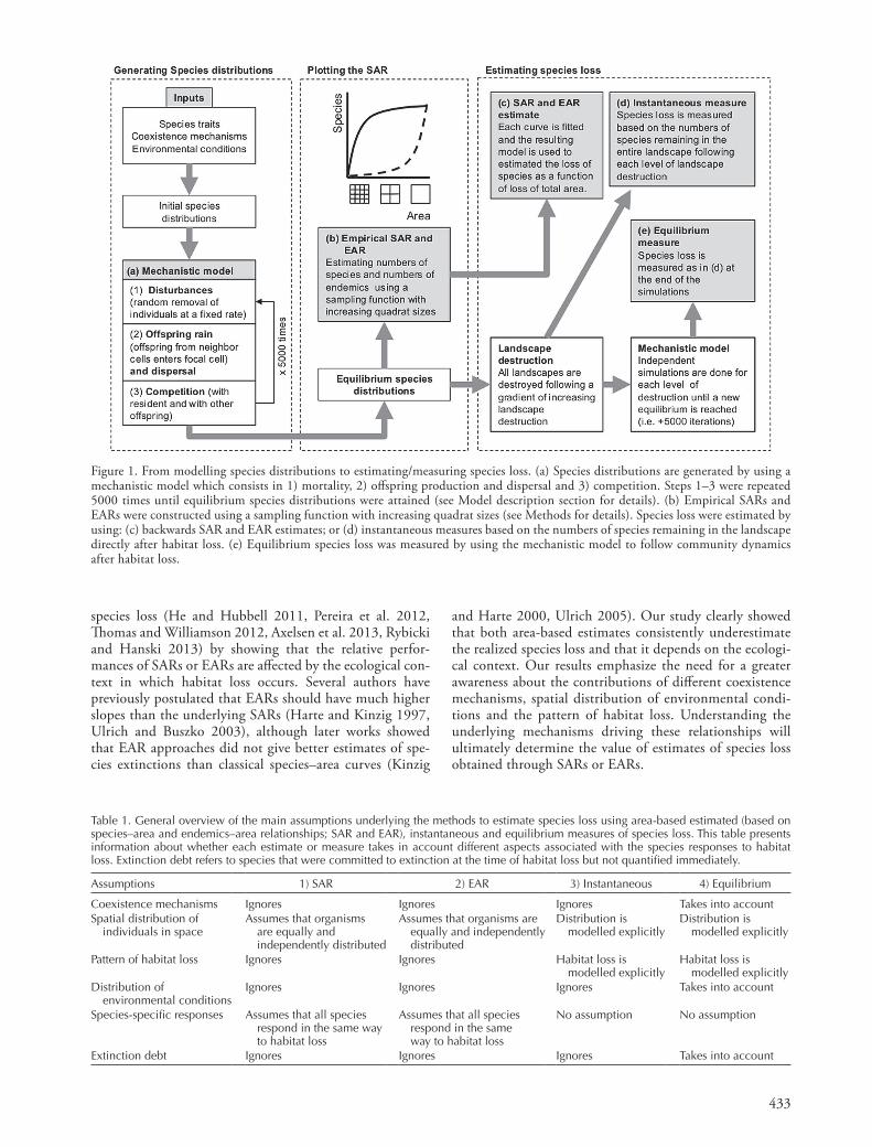
Figure 1. From modelling species distributions to estimating/measuring species loss. (a) Species distributions are generated by using a mechanistic model which consists in 1) mortality, 2) offspring production and dispersal and 3) competition. Steps 1–3 were repeated 5000 times until equilibrium species distributions were attained (see Model description section for details). (b) Empirical SARs and EARs were constructed using a sampling function with increasing quadrat sizes (see Methods for details). Species loss were estimated by using: (c) backwards SAR and EAR estimates; or (d) instantaneous measures based on the numbers of species remaining in the landscape directly after habitat loss. (e) Equilibrium species loss was measured by using the mechanistic model to follow community dynamics after habitat loss.
Table 1. General overview of the main assumptions underlying the methods to estimate species loss using area-based estimated (based on species–area and endemics–area relationships; SAR and EAR), instantaneous and equilibrium measures of species loss. This table presents information about whether each estimate or measure takes in account different aspects associated with the species responses to habitat loss. Extinction debt refers to species that were committed to extinction at the time of habitat loss but not quantified immediately.
Assumptions 1) SAR 2) EAR 3) Instantaneous 4) Equilibrium
Coexistence mechanisms Ignores Ignores Ignores Takes into accountSpatial distribution of
individuals in spaceAssumes that organisms
are equally and independently distributed
Assumes that organisms are equally and independently distributed
Distribution is modelled explicitly
Distribution is modelled explicitly
Pattern of habitat loss Ignores Ignores Habitat loss is modelled explicitly
Habitat loss is modelled explicitly
Distribution of environmental conditions
Ignores Ignores Ignores Takes into account
Species-specific responses Assumes that all species respond in the same way to habitat loss
Assumes that all species respond in the same way to habitat loss
No assumption No assumption
Extinction debt Ignores Ignores Ignores Takes into account
434
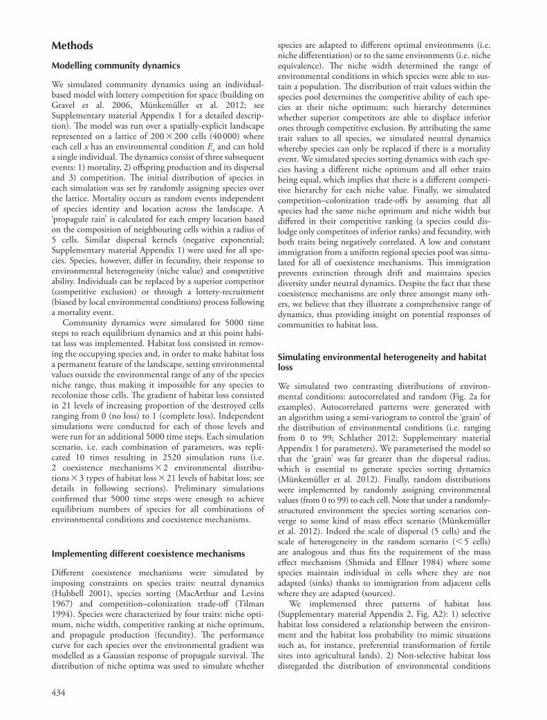
species are adapted to different optimal environments (i.e. niche differentiation) or to the same environments (i.e. niche equivalence). �e niche width determined the range of environmental conditions in which species were able to sus-tain a population. �e distribution of trait values within the species pool determines the competitive ability of each spe-cies at their niche optimum; such hierarchy determines whether superior competitors are able to displace inferior ones through competitive exclusion. By attributing the same trait values to all species, we simulated neutral dynamics whereby species can only be replaced if there is a mortality event. We simulated species sorting dynamics with each spe-cies having a different niche optimum and all other traits being equal, which implies that there is a different competi-tive hierarchy for each niche value. Finally, we simulated competition–colonization trade-offs by assuming that all species had the same niche optimum and niche width but differed in their competitive ranking (a species could dis-lodge only competitors of inferior ranks) and fecundity, with both traits being negatively correlated. A low and constant immigration from a uniform regional species pool was simu-lated for all of coexistence mechanisms. �is immigration prevents extinction through drift and maintains species diversity under neutral dynamics. Despite the fact that these coexistence mechanisms are only three amongst many oth-ers, we believe that they illustrate a comprehensive range of dynamics, thus providing insight on potential responses of communities to habitat loss.
Simulating environmental heterogeneity and habitat loss
We simulated two contrasting distributions of environ-mental conditions: autocorrelated and random (Fig. 2a for examples). Autocorrelated patterns were generated with an algorithm using a semi-variogram to control the ‘grain’ of the distribution of environmental conditions (i.e. ranging from 0 to 99; Schlather 2012; Supplementary material Appendix 1 for parameters). We parameterised the model so that the ‘grain’ was far greater than the dispersal radius, which is essential to generate species sorting dynamics (Münkemüller et al. 2012). Finally, random distributions were implemented by randomly assigning environmental values (from 0 to 99) to each cell. Note that under a randomly-structured environment the species sorting scenarios con-verge to some kind of mass effect scenario (Münkemüller et al. 2012). Indeed the scale of dispersal (5 cells) and the scale of heterogeneity in the random scenario ( 5 cells) are analogous and thus fits the requirement of the mass effect mechanism (Shmida and Ellner 1984) where some species maintain individual in cells where they are not adapted (sinks) thanks to immigration from adjacent cells where they are adapted (sources).
We implemented three patterns of habitat loss (Supplementary material Appendix 2, Fig. A2): 1) selective habitat loss considered a relationship between the environ-ment and the habitat loss probability (to mimic situations such as, for instance, preferential transformation of fertile sites into agricultural lands). 2) Non-selective habitat loss disregarded the distribution of environmental conditions
Methods
Modelling community dynamics
We simulated community dynamics using an individual-based model with lottery competition for space (building on Gravel et al. 2006, Münkemüller et al. 2012; see Supplementary material Appendix 1 for a detailed descrip-tion). �e model was run over a spatially-explicit landscape represented on a lattice of 200 200 cells (40 000) where each cell x has an environmental condition Ex and can hold a single individual. �e dynamics consist of three subsequent events: 1) mortality, 2) offspring production and its dispersal and 3) competition. �e initial distribution of species in each simulation was set by randomly assigning species over the lattice. Mortality occurs as random events independent of species identity and location across the landscape. A ‘propagule rain’ is calculated for each empty location based on the composition of neighbouring cells within a radius of 5 cells. Similar dispersal kernels (negative exponential; Supplementary material Appendix 1) were used for all spe-cies. Species, however, differ in fecundity, their response to environmental heterogeneity (niche value) and competitive ability. Individuals can be replaced by a superior competitor (competitive exclusion) or through a lottery-recruitment (biased by local environmental conditions) process following a mortality event.
Community dynamics were simulated for 5000 time steps to reach equilibrium dynamics and at this point habi-tat loss was implemented. Habitat loss consisted in remov-ing the occupying species and, in order to make habitat loss a permanent feature of the landscape, setting environmental values outside the environmental range of any of the species niche range, thus making it impossible for any species to recolonize those cells. �e gradient of habitat loss consisted in 21 levels of increasing proportion of the destroyed cells ranging from 0 (no loss) to 1 (complete loss). Independent simulations were conducted for each of those levels and were run for an additional 5000 time steps. Each simulation scenario, i.e. each combination of parameters, was repli-cated 10 times resulting in 2520 simulation runs (i.e. 2 coexistence mechanisms 2 environmental distribu-tions 3 types of habitat loss 21 levels of habitat loss; see details in following sections). Preliminary simulations confirmed that 5000 time steps were enough to achieve equilibrium numbers of species for all combinations of environmental conditions and coexistence mechanisms.
Implementing different coexistence mechanisms
Different coexistence mechanisms were simulated by imposing constraints on species traits: neutral dynamics (Hubbell 2001), species sorting (MacArthur and Levins 1967) and competition–colonization trade-off (Tilman 1994). Species were characterized by four traits: niche opti-mum, niche width, competitive ranking at niche optimum, and propagule production (fecundity). �e performance curve for each species over the environmental gradient was modelled as a Gaussian response of propagule survival. �e distribution of niche optima was used to simulate whether
435
confined to a particular sampling quadrat (He and Hubbell 2011). �e resulting empirical SAR and EAR curves describe how the average numbers of species or endemics change with the size of sampled quadrat within a given landscape (Fig. 2).
Estimating species loss
We estimated proportions of species loss with SARs and EARs following the principle that if the number of species (S) in an area (A) is characterized by a function S f (A), then it is possible to predict the number of species resulting from removing an area a from the initial total area. �is approach is often called the backward SAR estimate (He and Hubbell 2011), since it uses the generic SAR relationship to estimate the number of species for the remaining area, f (A–a). �e predicted number of extinct species following a given area of habitat loss a can be calculated as Sa(SAR) SA 2 S(A2a), where SA is initial species richness. �e propor-tion of species lost relative to the initial species richness is then lSAR Sa(SAR)/SA. �e lSAR takes values between 0 and 1. Values of 0 indicate that no species are expected to go extinct; values of 1 indicate that all species are expected to go extinct. We similarly characterized the EAR (E g(A)) and used it as
and consisted of a gradual spread of habitat loss across the landscape (e.g. volcano eruptions, indiscriminate deforesta-tion, etc). �is pattern of habitat loss was implemented with an algorithm using a semi-variogram as described before but with a grain of a 50-cell radius, with gradual and directional habitat loss (Supplementary material Appendix 2, Fig. A2). 3) Random habitat loss had no spatial structure and was implemented by randomly destroying cells. �ese three pat-terns of habitat loss were chosen to be illustrative of the major expectations of these factors and not an exhaustive exploration of either one of them (see Dytham 1995 for other patterns).
Generating SAR and EAR curves
We constructed empirical SAR and EAR curves by sampling simulated landscapes using a bisection procedure (Chave et al. 2002), such that each point in the curve represents the average number of species or endemics found in all non-overlapping quadrats of a given size that, collectively, cover the entire lattice. �is procedure was repeated with increas-ing quadrat size (i.e. 2 2, 3 3, 5 5 cells, etc.) until the size of the lattice was reached (i.e. 200 200 cells). We considered a species to be endemic when it was completely
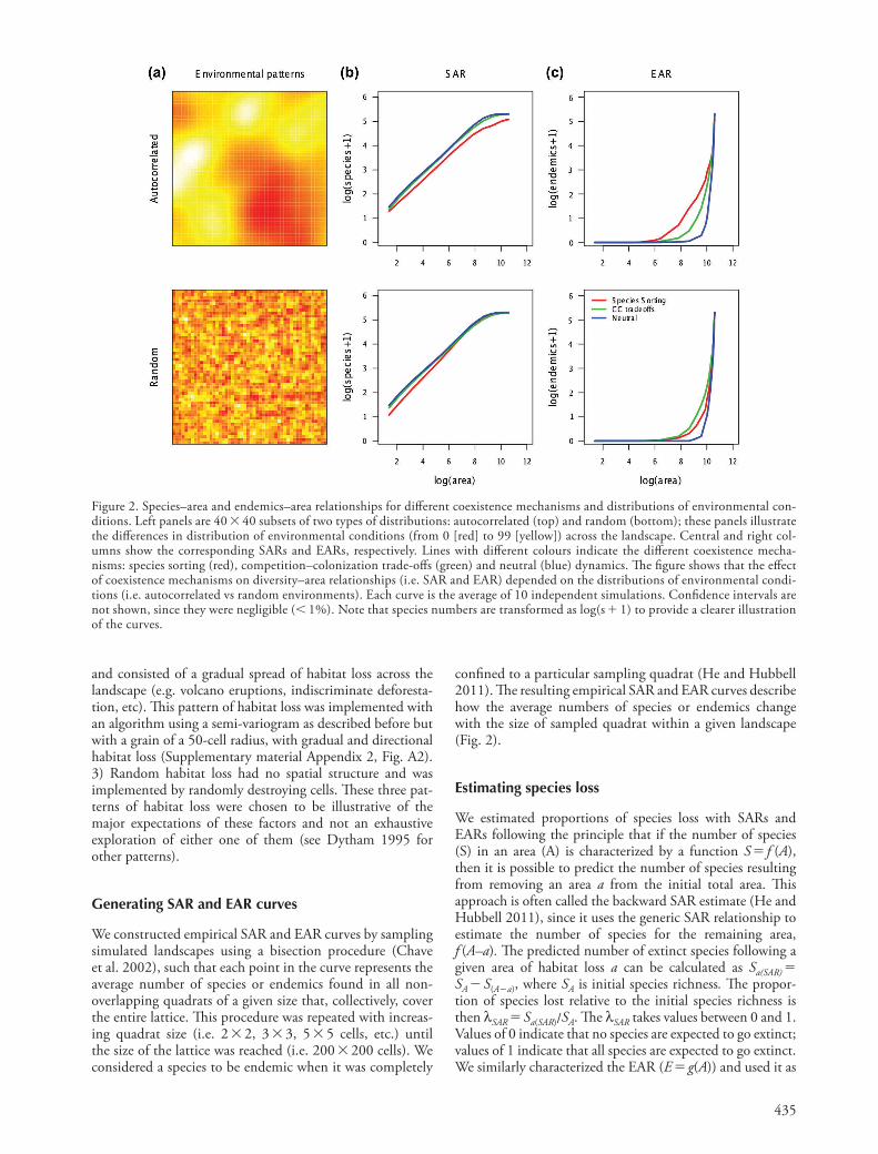
Figure 2. Species–area and endemics–area relationships for different coexistence mechanisms and distributions of environmental con-ditions. Left panels are 40 40 subsets of two types of distributions: autocorrelated (top) and random (bottom); these panels illustrate the differences in distribution of environmental conditions (from 0 [red] to 99 [yellow]) across the landscape. Central and right col-umns show the corresponding SARs and EARs, respectively. Lines with different colours indicate the different coexistence mecha-nisms: species sorting (red), competition–colonization trade-offs (green) and neutral (blue) dynamics. �e figure shows that the effect of coexistence mechanisms on diversity–area relationships (i.e. SAR and EAR) depended on the distributions of environmental condi-tions (i.e. autocorrelated vs random environments). Each curve is the average of 10 independent simulations. Confidence intervals are not shown, since they were negligible ( 1%). Note that species numbers are transformed as log(s 1) to provide a clearer illustration of the curves.
436
identical under trade-off and neutral dynamics regardless of the spatial structure of the environment. In communi-ties driven by species sorting species richness increased faster with area and reached higher values in random than in autocorrelated environments (Fig. 2b). When environ-mental conditions were randomly distributed, SARs exhib-ited similar shapes for all three coexistence mechanisms, with increases in species richness with area only slightly lower for trade-off dynamics at intermediate values of area (e.g. ~ 5000–20 000 grid cells; Fig. 2b). �e shape of the EAR was mediated by the coexistence mechanisms and the spatial structure of the environment. Under species sorting dynamics, endemic species became endemic earlier in auto-correlated (e.g. ~ 2000 grid cells; Fig. 2c) than in random environments (e.g. ~ 10 000 grid cells; Fig. 2c). �e EARs under neutral and trade-off dynamics were not sensi-tive to the spatial structure of the environment. Endemics were sampled faster under trade-off dynamics than under neutral community assembling (Fig. 2c). �e most notice-able differences due to the environmental patterns were observed under species sorting dynamics: the SARs grew faster in random environments because habitats were sampled faster than when environmental conditions (i.e. habitats) are autocorrelated and there is a closer coupling between distribution of species and types. �e opposite was true for the EAR as it grew faster in autocorrelated environments under species sorting dynamics.
Estimates and measures of species loss
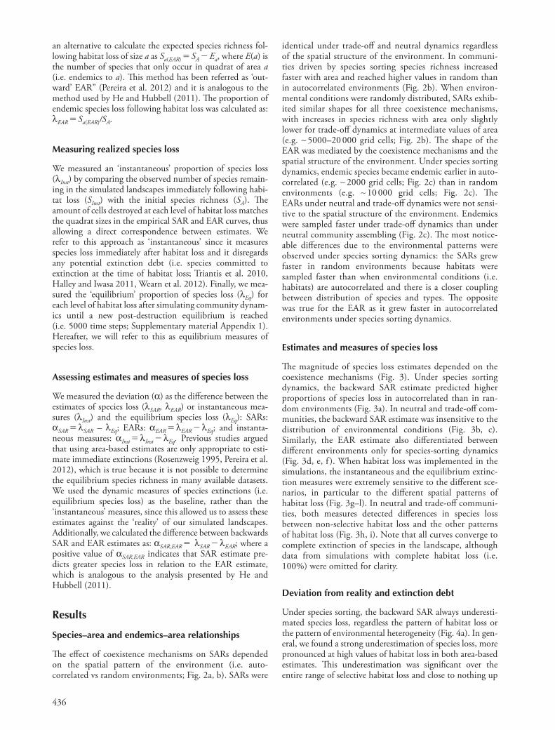
�e magnitude of species loss estimates depended on the coexistence mechanisms (Fig. 3). Under species sorting dynamics, the backward SAR estimate predicted higher proportions of species loss in autocorrelated than in ran-dom environments (Fig. 3a). In neutral and trade-off com-munities, the backward SAR estimate was insensitive to the distribution of environmental conditions (Fig. 3b, c). Similarly, the EAR estimate also differentiated between different environments only for species-sorting dynamics (Fig. 3d, e, f ). When habitat loss was implemented in the simulations, the instantaneous and the equilibrium extinc-tion measures were extremely sensitive to the different sce-narios, in particular to the different spatial patterns of habitat loss (Fig. 3g–l). In neutral and trade-off communi-ties, both measures detected differences in species loss between non-selective habitat loss and the other patterns of habitat loss (Fig. 3h, i). Note that all curves converge to complete extinction of species in the landscape, although data from simulations with complete habitat loss (i.e. 100%) were omitted for clarity.
Deviation from reality and extinction debt
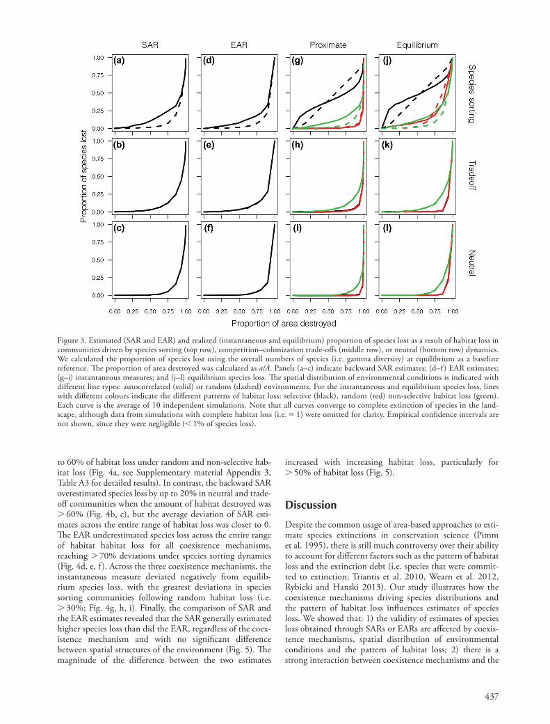
Under species sorting, the backward SAR always underesti-mated species loss, regardless the pattern of habitat loss or the pattern of environmental heterogeneity (Fig. 4a). In gen-eral, we found a strong underestimation of species loss, more pronounced at high values of habitat loss in both area-based estimates. �is underestimation was significant over the entire range of selective habitat loss and close to nothing up
an alternative to calculate the expected species richness fol-lowing habitat loss of size a as Sa(EAR) SA 2 Ea, where E(a) is the number of species that only occur in quadrat of area a (i.e. endemics to a). �is method has been referred as ‘out-ward’ EAR” (Pereira et al. 2012) and it is analogous to the method used by He and Hubbell (2011). �e proportion of endemic species loss following habitat loss was calculated as: lEAR Sa(EAR)/SA.
Measuring realized species loss
We measured an ‘instantaneous’ proportion of species loss (lInst) by comparing the observed number of species remain-ing in the simulated landscapes immediately following habi-tat loss (SInst) with the initial species richness (SA). �e amount of cells destroyed at each level of habitat loss matches the quadrat sizes in the empirical SAR and EAR curves, thus allowing a direct correspondence between estimates. We refer to this approach as ‘instantaneous’ since it measures species loss immediately after habitat loss and it disregards any potential extinction debt (i.e. species committed to extinction at the time of habitat loss; Triantis et al. 2010, Halley and Iwasa 2011, Wearn et al. 2012). Finally, we mea-sured the ‘equilibrium’ proportion of species loss (lEq) for each level of habitat loss after simulating community dynam-ics until a new post-destruction equilibrium is reached (i.e. 5000 time steps; Supplementary material Appendix 1). Hereafter, we will refer to this as equilibrium measures of species loss.
Assessing estimates and measures of species loss
We measured the deviation (a) as the difference between the estimates of species loss (lSAR, lEAR) or instantaneous mea-sures (lInst) and the equilibrium species loss (lEq): SARs: aSAR lSAR – lEq; EARs: aEAR lEAR 2 lEq; and instanta-neous measures: aInst lInst 2 lEq. Previous studies argued that using area-based estimates are only appropriate to esti-mate immediate extinctions (Rosenzweig 1995, Pereira et al. 2012), which is true because it is not possible to determine the equilibrium species richness in many available datasets. We used the dynamic measures of species extinctions (i.e. equilibrium species loss) as the baseline, rather than the ‘instantaneous’ measures, since this allowed us to assess these estimates against the ‘reality’ of our simulated landscapes. Additionally, we calculated the difference between backwards SAR and EAR estimates as: aSAR,EAR lSAR 2 lEAR; where a positive value of aSAR,EAR indicates that SAR estimate pre-dicts greater species loss in relation to the EAR estimate, which is analogous to the analysis presented by He and Hubbell (2011).
Results
Species–area and endemics–area relationships
�e effect of coexistence mechanisms on SARs depended on the spatial pattern of the environment (i.e. auto-correlated vs random environments; Fig. 2a, b). SARs were
437
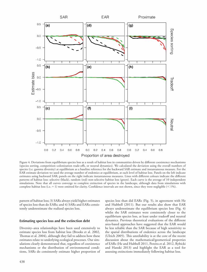
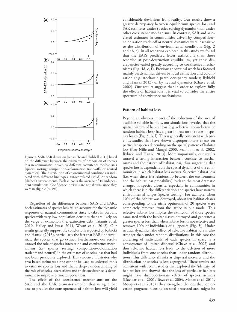
increased with increasing habitat loss, particularly for 50% of habitat loss (Fig. 5).
Discussion
Despite the common usage of area-based approaches to esti-mate species extinctions in conservation science (Pimm et al. 1995), there is still much controversy over their ability to account for different factors such as the pattern of habitat loss and the extinction debt (i.e. species that were commit-ted to extinction; Triantis et al. 2010, Wearn et al. 2012, Rybicki and Hanski 2013). Our study illustrates how the coexistence mechanisms driving species distributions and the pattern of habitat loss influences estimates of species loss. We showed that: 1) the validity of estimates of species loss obtained through SARs or EARs are affected by coexis-tence mechanisms, spatial distribution of environmental conditions and the pattern of habitat loss; 2) there is a strong interaction between coexistence mechanisms and the
to 60% of habitat loss under random and non-selective hab-itat loss (Fig. 4a, see Supplementary material Appendix 3, Table A3 for detailed results). In contrast, the backward SAR overestimated species loss by up to 20% in neutral and trade-off communities when the amount of habitat destroyed was 60% (Fig. 4b, c), but the average deviation of SAR esti-mates across the entire range of habitat loss was closer to 0. �e EAR underestimated species loss across the entire range of habitat habitat loss for all coexistence mechanisms, reaching 70% deviations under species sorting dynamics (Fig. 4d, e, f ). Across the three coexistence mechanisms, the instantaneous measure deviated negatively from equilib-rium species loss, with the greatest deviations in species sorting communities following random habitat loss (i.e. 30%; Fig. 4g, h, i). Finally, the comparison of SAR and the EAR estimates revealed that the SAR generally estimated higher species loss than did the EAR, regardless of the coex-istence mechanism and with no significant difference between spatial structures of the environment (Fig. 5). �e magnitude of the difference between the two estimates
Figure 3. Estimated (SAR and EAR) and realized (instantaneous and equilibrium) proportion of species lost as a result of habitat loss in communities driven by species sorting (top row), competition–colonization trade-offs (middle row), or neutral (bottom row) dynamics. We calculated the proportion of species lost using the overall numbers of species (i.e. gamma diversity) at equilibrium as a baseline reference. �e proportion of area destroyed was calculated as a/A. Panels (a–c) indicate backward SAR estimates; (d–f ) EAR estimates; (g–i) instantaneous measures; and (j–l) equilibrium species loss. �e spatial distribution of environmental conditions is indicated with different line types: autocorrelated (solid) or random (dashed) environments. For the instantaneous and equilibrium species loss, lines with different colours indicate the different patterns of habitat loss: selective (black), random (red) non-selective habitat loss (green). Each curve is the average of 10 independent simulations. Note that all curves converge to complete extinction of species in the land-scape, although data from simulations with complete habitat loss (i.e. 1) were omitted for clarity. Empirical confidence intervals are not shown, since they were negligible ( 1% of species loss).
438
Figure 4. Deviations from equilibrium species loss as a result of habitat loss in communities driven by different coexistence mechanisms (species sorting, competition–colonization trade-offs, or neutral dynamics). We calculated the deviation using the overall numbers of species (i.e. gamma diversity) at equilibrium as a baseline reference for the backward SAR estimate and instantaneous measure. For the EAR estimate deviation we used the average number of endemics at equilibrium, at each level of habitat loss. Panels on the left indicate estimates using backward SAR; panels on the right indicate instantaneous measures. Lines with different colours indicate the different patterns of habitat loss: selective (black), random (red) non-selective habitat loss (green). Each curve is the average of 10 independent simulations. Note that all curves converge to complete extinction of species in the landscape, although data from simulations with complete habitat loss (i.e. 1) were omitted for clarity. Confidence intervals are not shown, since they were negligible ( 1%).
pattern of habitat loss; 3) SARs always yield higher estimates of species loss than do EARs; and 4) SARs and EARs consis-tently underestimate the realized species loss.
Estimating species loss and the extinction debt
Diversity–area relationships have been used extensively to estimate species loss from habitat loss (Brooks et al. 2002, �omas et al. 2004), although they fail to address how these estimates relate to underlying ecological processes. Our sim-ulations clearly demonstrated that, regardless of coexistence mechanisms or the distribution of environmental condi-tions, SARs do consistently estimate higher proportion of
species loss than did EARs (Fig. 5), in agreement with He and Hubbell (2011). But our results also show that EAR always underestimate the equilibrium species loss (Fig. 4) whilst the SAR estimates were consistently closer to the equilibrium species loss, at least under tradeoff and neutral dynamics. Previous theoretical evaluations of the different area-based approaches have suggested that the EAR would be less reliable than the SAR because of high sensitivity to the spatial distributions of endemics across the landscape (Ulrich 2005). �is unreliability is at the core of the recent discussion about the mathematical/geometrical properties of EARs (He and Hubbell 2011, Pereira et al. 2012, Rybicki and Hanski 2013) and highlight the EAR as a tool for assessing extinctions immediately following habitat loss.
439
considerable deviations from reality. Our results show a greater discrepancy between equilibrium species loss and SAR estimates under species sorting dynamics than under other coexistence mechanisms. In contrast, SAR and asso-ciated estimates in communities driven by competition– colonization trade-off or neutral dynamics were insensitive to the distribution of environmental conditions (Fig. 2 and 4b, c). In all scenarios explored in this study we found that the EARs predicted fewer extinctions than those recorded at post-destruction equilibrium, yet these dis-crepancies varied greatly according to coexistence mecha-nisms (Fig. 4d, e, f ). Previous theoretical work has focused mainly on dynamics driven by local extinction and coloni-zation (e.g. stochastic patch occupancy models; Rybicki and Hanski 2013) or by neutral dynamics (Chave et al. 2002). Our results suggest that in order to explore fully the effects of habitat loss it is vital to consider the entire spectrum of coexistence mechanisms.
Pattern of habitat loss
Beyond an obvious impact of the reduction of the area of available suitable habitats, our simulations revealed that the spatial pattern of habitat loss (e.g. selective, non-selective or random habitat loss) has a great impact on the rates of spe-cies losses (Fig. 3j, k, l). �is is generally consistent with pre-vious studies that have shown disproportionate effects on particular species depending on the spatial pattern of habitat loss (Ney-Nifle and Mangel 2000, Seabloom et al. 2002, Rybicki and Hanski 2013). More importantly, our results unravel a strong interaction between coexistence mecha-nisms and the pattern of habitat loss, thus suggesting that species loss is dependent on the spatial dynamics of the com-munities in which habitat loss occurs. Selective habitat loss (i.e. when there is a relationship between the environment and the habitat loss probability) leads to the most dramatic changes in species diversity, especially in communities in which there is niche differentiation and species have narrow environmental ranges (species sorting). For example, when 10% of the habitat was destroyed, about ten habitat classes corresponding to the niche optimums of 20 species were completely removed from the lattice in our model. �is selective habitat loss implies the extinction of those species associated with the habitat classes destroyed and generates a greater species loss than when habitat loss is not selective and removes 10% of individuals of all species (Fig. 3j). Under neutral dynamics, the effect of selective habitat loss is also stronger than under random distributions. In this case the clustering of individuals of each species in space is a consequence of limited dispersal (Chave et al. 2002) and thus selective habitat loss leads to the deletion of more individuals from one species than under random distribu-tions. �is difference shrinks as dispersal increases and the distribution of species is less aggregated. �ese results are consistent with recent studies that explored the ‘identity’ of habitat lost and showed that the loss of particular habitats might have disproportionate effects of species richness (Davidar et al. 2001, Tews et al. 2004, Matias et al. 2011, Mouquet et al. 2013). �ey strengthen the idea that conser-vation programs focusing on total protected area might be
Figure 5. SAR-EAR deviation (sensu He and Hubbell 2011) based on the difference between the estimates of proportion of species loss in communities driven by different coexistence mechanisms (species sorting, competition–colonization trade-offs, or neutral dynamics). �e distribution of environmental conditions is indi-cated with different line types: autocorrelated (solid) or random (dashed) environments. Each curve is the average of 10 indepen-dent simulations. Confidence intervals are not shown, since they were negligible ( 1%).
Regardless of the differences between SARs and EARs, both estimates of species loss fail to account for the dynamic responses of natural communities since it takes in account species with very low population densities that are likely on the verge of extinction (i.e. extinction debt; Triantis et al. 2010, Halley and Iwasa 2011, Wearn et al. 2012). Our results generally support the conclusions reported by Rybicki and Hanski (2013), particularly the fact that EAR underesti-mate the species that go extinct. Furthermore, our results unravel the role of species interaction and coexistence mech-anisms (i.e. species sorting, competition–colonization tradeoff and neutral) in the estimates of species loss that had not been previously explored. �is evidence illustrates why area-based estimates alone cannot be used as universal tools to estimate species loss and that a deeper understanding of the role of species interactions and their coexistence is deter-minant to improve estimate species loss.
�e effect of the coexistence mechanisms on the SAR and the EAR estimates implies that using either one to predict the consequences of habitat loss will yield
440
SARs and EARs to forecast the consequences of habitat loss under different ecological contexts in the field. �is will require incorporating knowledge about species’ responses at the appropriate biological and ecological scales. It might sound very ambitious but it fits the urgency of understanding the consequences of habitat loss, proba-bly the major driver of species extinction today, far beyond climatic changes.
Moving towards realistic estimates of species loss
It seems clear that neither SARs nor EARs alone can be used as universal tools to estimate species loss (He and Hubbell 2011) and that it is necessary to develop more complex methods incorporating ecological processes to complement the predictions from area-based methods. One promising approach to explicitly incorporate various aspects of the ecological context is to use process-based distribution models (�uiller et al. 2013). Process-based models predict species distributions by combining habitat-suitability models (e.g. climatic or land-cover suitability) with either demographic (e.g. coupled niche-population models; Anderson et al. 2009, Brook et al. 2009) or physi-ological (Kearney and Porter 2009) data. �e success of these process-based approaches is often undermined by the scarcity of information available to calibrate the models (e.g. survival rates and dispersal rates), which in turn limits the application of process-based models beyond specific case studies (Brook et al. 2009). Despite the large number of parameters required for such models, it is nonetheless possible to parameterize them for a reasonable number of species and have a first-order approximation of biodiversity loss under various scenarios (Pereira et al. 2012). Alternatively, neutral models have been already used to pre-dict species distributions and estimate tree species extinc-tions in the Amazonian forest (Hubbell et al. 2008). �ese neutral-based approaches may have some unrealistic assumptions but they represent the opposite end of the spectrum, thus providing an alternative set of predictions that can be very useful to contrast with niche-based approaches. �e combination of such different modelling approaches could be used to generate envelopes of uncer-tainty around baseline predictions from traditional area-based estimates. Devising a new comprehensive framework to estimate species loss that is based on ecological mecha-nisms, and not solely on distributional patterns, should be at the forefront of future ecological discussions.
Acknowledgements – MM was supported by the grant ANR-BACH-09-JCJC-0110-01, ML by the TULIP Laboratory of Excellence (ANR-10-LABX-41), NM by the CNRS. TM was funded by the ANR-BiodivERsA project CONNECT (ANR-11-EBID-002), as part of the ERA-Net BiodivERsA 2010 call. DG and PDP were supported by NSERC and the Canada Research Chair program. TM, DG and NM received additional support from DIVERSITALP Project (ANR-07-BDIV-014). FG was supported by the ‘Range Shift’ project (PTDC/AAC-AMB/098163/2008) from Fundação para a Ciência e a Tecnologia (Portugal), co-financed by the European Social Fund. �e ‘Rui Nabeiro’ Biodiversity Chair is financed by Delta Cafés. We thank Miguel Araújo, Joaquin Hortal, and Kostas Triantis for constructive comments.
counterproductive as opposed to conservation strategies accounting for different habitats types when communities are strongly driven by species sorting dynamics.
From virtual landscapes back to reality
Our simulation approach allowed us to measure equilibrium species loss and therefore to quantify the deviation of area-based estimates (SAR and EARs) of species loss from actual extinctions after community dynamics has taken place. �is method was used to illustrate how the SAR and the EAR were ‘performing’, rather than using empirical datasets because 1) it is very difficult to determine ongoing species loss in the field and 2) the extinction debt might last for long. Our interpretation of these results is necessarily grounded on the underlying assumptions of each of the sim-ulated community assembly processes, which generated extremely simple communities that represents only extreme cases and are unlikely to encapsulate natural complexities. Our implementation of habitat habitat loss was also quite conservative since it assumes that habitat loss leads to com-pletely unsuitable habitats for all species, which is rarely the case as it is known that many species can establish popula-tions in various habitat types (Pereira and Daily 2006) and survive in human modified habitats (e.g. ‘urban exploiters’ McKinney 2002). Despite these constraints, we believe that these results are stimulating for the discussions on estimates of species loss and on the consequences of habitat loss on biodiversity.
As regards empirical studies, the ongoing development of global databases and time-series of both species distri-butions and historical sequences of land-use change is a promising line of research to investigate the effects of hab-itat loss (Triantis et al. 2010). However, most existing datasets and corresponding correlative studies are unlikely to provide unequivocal evidence for linking particular events of habitat loss to the extinction of particular spe-cies, or to allow quantifying the time lag between loss and extinction. As habitat size determines the time needed for communities to reach equilibrium (Mouquet et al. 2003), it is likely that the magnitude and velocity of habitat loss will determine the post-destruction speed of community dynamics, thus affecting the time lag in biotic responses, which are also likely to be functions of the coexistence mechanisms driving the communities. Addressing these limitations in order to achieve a comprehensive under-standing of the consequences of habitat loss will probably come from combining empirical knowledge and experi-mental approaches. �is can be done, for instance, by test-ing theoretical predictions using known experimental landscapes such as mosses (Gonzalez et al. 1998), sandy-bottoms (Bulling et al. 2008); macroalgae (Matias et al. 2011) and seagrasses (Macreadie et al. 2009). �e organ-isms colonizing these model systems often have relatively small sizes and short generation times, which makes them highly tractable to experimental manipulation (see review in Logue et al. 2011) and for measuring dynamic responses to habitat loss. Long-term empirical experiments will also be needed over larger scales for habitats such as forests, coral reefs and grasslands to determine the relevance of
441
Julliard, R. et al. 2004. Common birds facing global changes: what makes a species at risk? – Global Change Biol. 10: 148–154.
Kearney, M. and Porter, W. 2009. Mechanistic niche modelling: combining physiological and spatial data to predict species’ ranges. – Ecol. Lett. 12: 334–350.
Kelly, C. K. et al. 2008. Phylogeny, niches, and relative abundance in natural communities. – Ecology 89: 962–970.
Kinzig, A. P. and Harte, J. 2000. Implications of endemics–area relationships for estimates of species extinctions. – Ecology 81: 3305–3311.
Logue, J. B. et al. 2011. Empirical approaches to metacommunities: a review and comparison with theory. – Trends Ecol. Evol. 26: 482–491.
MacArthur, R. H. and Levins, R. 1967. Limiting similarity convergence and divergence of coexisting species. – Am. Nat. 101: 377–385.
MacArthur, R. H. and Wilson, E. O. 1967. �e theory of island biogeography. – Princeton Univ. Press.
Macreadie, P. I. et al. 2009. Fish responses to experimental fragmentation of seagrass habitat. – Conserv. Biol. 23: 644–652.
Matias, M. G. et al. 2011. Habitat identity influences endemics–area relationships in heterogeneous habitats. – Mar. Ecol. Prog. Ser. 437: 135–145.
May, R. M. et al. 1995. Assessing extinction rates. – In: Lawton, J. H. and May, R. M. (eds), Extinction rates. Oxford Univ. Press, pp. 1–24.
McGill, B. J. et al. 2007. Species abundance distributions: moving beyond single prediction theories to integration within an ecological framework. – Ecol. Lett. 10: 995–1015.
McKinney, M. L. 2002. Urbanization, biodiversity, and conservation. – Bioscience 52: 883–890.
McKinney, M. L. and Lockwood, J. L. 1999. Biotic homogeni-zation: a few winners replacing many losers in the next mass extinction. – Trends Ecol. Evol. 14: 450–453.
Mouquet, N. et al. 2003. Community assembly time and the relationship between local and regional species richness. – Oikos 103: 618–626.
Mouquet, N. et al. 2013. Extending the concept of keystone species to communities and ecosystems. – Ecol. Lett. 16: 1–8.
Münkemüller, T. et al. 2012. From diversity indices to community assembly processes: a test with simulated data. – Ecography 35: 468–480.
Ney-Nifle, M. and Mangel, M. 2000. Habitat loss and changes in the endemics–area relationship. – Conserv. Biol. 14: 893–898.
Pereira, H. M. and Daily, G. C. 2006. Modeling biodiversity dynamics in countryside landscapes. – Ecology 87: 1877–1885.
Pereira, H. M. et al. 2012. Geometry and scale in endemics–area relationships. – Nature 482: E3–E4.
Pimm, S. L. et al. 1995. �e future of biodiversity. – Science 269: 347–350.
Rosenzweig, M. L. 1995. Species diversity in space and time. – Cambridge Univ. Press.
Rybicki, J. and Hanski, I. 2013. Species–area relationships and extinctions caused by habitat loss and fragmentation. – Ecol. Lett. 16: 27–38.
Schlather, M. 2012. RandomFields: simulation and analysis of random fields. – R package ver. 2.0.54.
Seabloom, E. W. et al. 2002. Extinction rates under nonrandom patterns of habitat loss. – Proc. Natl Acad. Sci. USA 99: 11229–11234.
Shmida, A. and Ellner, S. 1984. Coexistence of plant species with Similar niches. – Vegetatio 58: 29–55.
DM, NM and MGM formulated the ideas; MGM, DG, TM and PDP implemented the modelling framework and run simulations; MGM and FG conducted data analysis; all the authors contributed for structuring and writing the paper.
References
Anderson, B. J. et al. 2009. Dynamics of range margins for metapopulations under climate change. – Proc. R. Soc. B 276: 1415–1420.
Axelsen, J. B. et al. 2013. Species–area relationships always overestimate extinction rates from habitat loss: comment. – Ecology 94: 761–763.
Benton, T. G. et al. 2003. Farmland biodiversity: is habitat heterogeneity the key? – Trends Ecol. Evol. 18: 182–188.
Brook, B. W. et al. 2009. Integrating bioclimate with population models to improve forecasts of species extinctions under climate change. – Biol. Lett. 5: 723–725.
Brooks, T. M. et al. 2002. Habitat loss and extinction in the hotspots of biodiversity. – Conserv. Biol. 16: 909–923.
Bulling, M. et al. 2008. Species effects on ecosystem processes are modified by faunal responses to habitat composition. – Oecologia 158: 511–520.
Chase, J. M. 2005. Towards a really unified theory for metacommunities. – Funct. Ecol. 19: 182–186.
Chave, J. et al. 2002. Comparing classical community models: theoretical consequences for patterns of diversity. – Am. Nat. 159: 1–23
Connor, E. F. and McCoy, E. D. 1979. �e statistics and biology of the species–area relationship. – Am. Nat. 113: 791–833.
Davidar, P. et al. 2001. Distribution of forest birds in the Andaman islands: importance of key habitats. – J. Biogeogr. 28: 663–671.
Dytham, C. 1995. �e effect of habitat destruction pattern on species persistence: a cellular model. – Oikos 74: 340–344.
Gonzalez, A. et al. 1998. Metapopulation dynamics, abundance, and distribution in a microecosystem. – Science 281: 2045–2047.
Gravel, D. et al. 2006. Reconciling niche and neutrality: the continuum hypothesis. – Ecol. Lett. 9: 399–409.
Halley, J. M. and Iwasa, Y. 2011. Neutral theory as a predictor of avifaunal extinctions after habitat loss. – Proc. Natl Acad. Sci. USA 108: 2316–2321.
Harte, J. and Kinzig, A. P. 1997. On the implications of species–area relationships for endemism, spatial turnover, and food web patterns. – Oikos 80: 417–427.
He, F. 2012. Area-based assessment of extinction risk. – Ecology 93: 974–980.
He, F. and Legendre, P. 2002. Species diversity patterns derived from species–area models. – Ecology 83: 1185–1198.
He, F. and Hubbell, S. P. 2011. Species–area relationships always overestimate extinction rates from habitat loss. – Nature 473: 368–371.
Heywood, V. H. 1995. �e global biodiversity assessment. United Nations Environment Programme. – Cambridge Univ. Press.
Holyoak, M. and Loreau, M. 2006. Reconciling empirical ecology with neutral community models. – Ecology 87: 1370–1377.
Hubbell, S. P. 2001. �e unified neutral theory of species abundance and diversity. – Princeton Univ. Press.
Hubbell, S. P. et al. 2008. How many tree species are there in the Amazon and how many of them will go extinct? – Proc. Natl Acad. Sci. USA 105: 11498–11504.
442
Triantis, K. A. et al. 2010. Extinction debt on oceanic islands. – Ecography 33: 285–294.
Ulrich, W. 2005. Predicting species numbers using species – area and endemics – area relations. – Biodivers. Conserv. 14: 3351–3362.
Ulrich, W. and Buszko, J. 2003. �e species–area relationship of butterflies in Europe: the simulation of extinction processes reveals different patterns between northern and southern Europe. – Ecography 26: 365–374.
Wearn, O. R. et al. 2012. Extinction debt and windows of conservation opportunity in the Brazilian Amazon. – Science 337: 228–232.
Tews, J. et al. 2004. Animal species diversity driven by habitat heterogeneity/diversity: the importance of keystone structures. – J. Biogeogr. 31: 79–92.
�omas, C. D. and Williamson, M. 2012. Extinction and climate change. – Nature 482: E4–E5.
�omas, C. D. et al. 2004. Extinction risk from climate change. – Nature 427: 145–148.
�uiller, W. et al. 2013. A road map for integrating eco- evolutionary processes into biodiversity models. – Ecol. Lett. 16: 94–105.
Tilman, D. 1994. Competition and biodiversity in spatially structured habitats. – Ecology 75: 2–16.
Supplementary material (Appendix ECOG-00448 at www.oikosoffice.lu.se/appendix ). Appendix 1–3.