. I .. I I l I I

r

Establishing a Statistical Criterion for Selecting Trip Generation Procedures HAROLD D. DEUTSCHMAN, Transportation Engineer,

Tri-State Transportation Commission

•TRIP generation procedures as used by regional transportation studies involve the systematic explanation of the relationship between the dependent variables (person trips per household and autos available per household) and the independent measures of social, economic, and household activities. Predicti:ve equations relating travel characteristics to the behavior of the household (measuring the travel demands of the households) are part of the basis for the systematic planning of the network of highways and mass transit facilities to meet t~is demand.

The intent of this study is to examine the independent variables used in the trip gen­eration process in the context of a developed criterion in order to choose the best single variable or combination of variables to most efficiently forecast the dependent variables of person trips per household and autos per household. Much attention is devoted to the establishment and development of a criterion to measure how closely the prediction ap­proximates reality. Sources of error examined in the forecasting process include (a) errors in estimating the independent variables, (b) errors in the simulation of the de­pendent variables for present-day conditions, and (c) errors in the forecasting equation using the independent variables. It is the joint effect of these three sources of error that produces the actual error of estimate. A minimization of this joint error is es­tablished as the standard for selecting the "best" trip generation procedure.

Preliminary findings from the Tri-State Transportation Commission are used to analyze the three types of errors and to point out the sensitivity of selection and the decision-making process of the analyst in selecting the most effective variables for trip generation purposes. In addition, auto registration and census data for the New York Metropolitan Area for the years 1950 and 1960 are used as a data base to analyze the error in the trip generation equation when used as a predictive device .

DEVELOPING THE CRITERION

A systematic approach in a trip generation process is to select an equation and/or model of n number of indep~ndent variables vs the dependent variables of person trips and autos per household. These equations are then tested against survey data to see how well they reproduce the data, the figure of merit usually consisting of the standard error of estimate and the coefficient of correlation. The next step is to examine the procedure to see if it logically may be used as a predictive device. The values of the independent variable must, of course, change over time at approximately the same rate as the dependent variable. It is not unusual to have a condition whereby an independent variable reproduces the survey data very well but fails completely when used for fore­casting purposes. A third step in the trip generating process is to estimate how accu­rately and to what geographic level of detail the independent variables may be estimated. There would be a trade-off, of course, between (a) choosing an independent variable yielding an excellent correlation with the dependent variable but being difficult to esti­mate and (b) selecting a variable which is easy to estimate but which has only a fair-to­good correlation with the dependent variable. A fourth step in the procedure is to com­pute the joint error of the three sources of error described, with the statistical

Paper sponsored by Committee on Origin and Destination and presented at the 46th Annual Meeting.

39

•.

40

SELECT INDEPENDENT VARIABLES THAT

ARE CAUSAL FACTORS IN SIMULATING

THE DEPENDE!IT VARIABLE

SELECT ONE INDEPENDENT VARIABLE

OR A LOGICAL COMBINATION

OF VARIABLES

MEASURE THE EFFECT OF THE INDEPENDENT

VARIABLES ON TIIE DEPENDENT VARIABLE

USE STANDARD ERROR OF ESTIMATE

USING PROCEDURE DEVELOPED TO ESTIMATE

THE INDEPENDENT VARIABLES, TEST PROCESS ON OLD

SURVEY DATA OR ON CENSUS DATA FOR 2

POlNTS IN TIME

(A)

MEASURE TIIE JOINT ERROR OF ESTIMATE

FROM(]) ERROR IN ESTIMATING INDEPENDENT VARIABLES &

a> ERROR IN ESTIMATING EQUATION.

(B)

MEASURE THE TOTAL ERROR OF ESTIMATE (STEPS A&B)

SELECT PROCEDURE & VARIABLES THAT

~IINIMIZE TOTAL ERROR DUE TO

Q) ESTIMATING INDEPENDENT VARIABLE

Q) SIMULATING DEPENDENT VARIABLE FOR PRESENT CONDITIONS

(})USE AS PREDICTIVE DEVICE

Figure 1. Flow chart for the selection of a statistical criterion for selecting trip generation procedures.

I 1. i I ~

l

I I

t

• 1

I ·I

I •

I

I . ·;

·1

I I I I

; ...

41

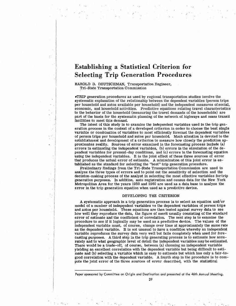
criterion for selecting a procedure simply consisting of a minimization of this joint error of estimate. A schematic diagram detailing this procedure is shown in Figure 1. The formula for calculating the joint error of estimate is as follows:

ERROR joint =

error2

in estimation

of independent variables

+

error2

in estimation equation to

simulate de -pendent variable

+

error2

in predictive power of equation

over time

ERROR IN SIMULATING DEPENDENT VARIABLES FOR PRESENT-DAY CONDITIONS

Reproducing the Survey Data

Transportation studies spend much attention in determining how well their indepen­dent variables reproduce the survey data's dependent variables. The measurement of the intensity of the effect of the independent variables on the dependent variables of per­son trips per household and autos available per household is usually made by the sta­tistical measures of the standard error of estimate and the coefficient of correlation . For the purposes of this analysis, the standard error of estimate will be used as the "error" measurement.

Preliminary findings from the Tri-State Transportation Commission are used to examine the variables for the error generated in reproducing the survey data. In ex­panding the Tri-State home interview survey, the study area was divided into 278 ex­pansion areas which are composed of groups 01 census tracts, municipalities, and groups of municipalities. These area~ are used as zones for trip generation equations in which data are available on person trips, auto availability, household characteristics, and density measures.

Trip generation rates were derived by using linear relationships between the de­pendent and independent variables. When necessary the variables were transformed to obtain this linear relationship (i.e., logarithm of gross density). Sets of equations were developed with the following independent and dependent variables:

Dependent Variable

(Xi) Person trips/household

(X:i) Vehicles/household

Independent Variable (s)

(X:i) Vehicles/household (L) Median household income (Xe) Percent single unit structures (X7) Log of gross residential density (:XS) Persons 5 years and older/household

(L), (Xe), (X7), (:XS)

In addition, linear combinations of the independent variables were tested against the two dependent variables. The results of this analysis are described below.

Dependent Variable-Person Trips per Household

The best single independent variable for estimating person trips for the survey data is vehicles per household, with the density measure of percent single unit structures ranking second while yielding a slightly greater e'rror. The ranking of the independent variables, using the standard' error of estimate divided by the mean of the dependent variable as a criterion for ranking, is as follows:

·.

42

· ..

Independent Variable

Vehicles per household Percent single unit structures Log of gross residential density Persons 5 years and older per household Median household income

S/X1 (Expressed as Percent)

15 17 21 31 32

When vehicles per household is linearly combined with percent single unit structures, the standard error of estimate for estimating person trips is reduced to 14 percent, and when persons 5 years and older is added to these two variables, the standard error of estimate is reduced to 13 percent.

Dependent Variable-Vehicles per Household

The most efficient sole determinant of vehicles per household is a measure of resi­dential density. Percent single unit structures and the logarithm of gross density, both approximations of residential density, yield the same magnitude of error (22 percent), while indicators of income and persons per household each produce about 2 times this error. The linear combination of (i.e., logarithm of) gross density and median house­hold income reduces this error of estimate to 19 percent while the inclusion of persons per household with these two independent variables yields an error of 18 percent.

The ranking of the independent variables by their associated standard error of esti­mate in estimating vehicles per household is as follows:

Independent Variable

Percent single unit structures Log of gross residential density Median household income Persons 5 years and older per household

S/X1 (Expressed as Percent)

22 22 43 45

I. t

.. ,

...

I .

The equations for the regression lines and corresponding errors of estimate are l · , detailed in Tables 1 and 2 of the Appendix for the dependent variables of vehicles per household and person trips per household.

ESTIMATION OF INDEPENDENT v ARIABLES I. There has not been a great deal of analytical work published by transportation plan- f ·

ning groups on determining the error in estimating independent variables or predictors. The ideal case would be to set up a zonal system equivalent to the one planned for use in the forecasting process, and then make use of census data for 1950 and 1960 or pre-vious surveys taken in the area to serve as the test of how well the independent vari- I ables may be estimated. Testing of this estimating process should be initiated even I . though data may be scarce or available only on a coarse geographic level.

It is generally agreed by analysts in the transportation field that the independent variables may be ranked by the ease and efficiency of estimation as follows: (a) popula­tion-related data; (b) density-related data, i.e., persons per residential area; (c) com­bination of population and density data, i. e., persons per household; and (d) income, i.e., median household income.

For the purposes of this paper, a hypothetical structure is created to measure the sensitivity of the error in estimating the independent variables on the efficiency of re­producing the survey data. The joint error of estimate from these two sources is cal­culated for an array of assumed errors of estimation for the independent variables.

The hypothetical structure used for analysis is based on a perturbation of the data from the Tri-State Transportation home interview survey in which (for purposes of ex­pansion) the study area was divided into 278 zones. An error of estimation was applied to the independent variables (income, density, and vehicle measures), this error being

·' ·'

.·

I

.. I . !

I

I ' . ,

;

43

a constant percentage of the actual zonal value, its sign (plus or minus) generated by a random number index. The following variables served as a basis for testing selected sets of equations:

Dependent Variable

(S1) Person trips/household (S2) Vehicles/household

Illustration of Perturbation Procedure

Independent Variables

(Ss.) Vehicles/household (0 % error) (S4) Vehicles/household (15 % error) (Ss) Percent single family units (O % error) (Ss) Percent single family units (10 % error) (S7) Median household income (O % error) (Se) Median household income (10 % error) (Se) Median household income (20 % error) (S10) Median household income (25 % error)

Independent Variable-Median Household Income, 10% Error (Se)

Sign of Error New Value of Actual (Survey) (Generated by Random Income With

Zone Value of Income (S7) Number Index) 10% Error (Se)

1 $5000 + $5500 2 $5500 + $6050 3 $6000 $5400 4 $4000 + $4400 5 $4500 $4050 6 $9000 $8100 7 $8200 + $9020

The (joint) error of reproducing the survey and in estimating the independent vari­ables was determined in a single calculation by running the (same) regression analysis with fixed errors in the independent variables.

Vehicles per Household

Assuming that a realistic figure for the error in estimating percent single family units is ±10 percent and the error in estimating median household income is in the range of ±20-25 percent, then either the use of (a) density as a sole variable for esti­mating vehicles per household, or (b) the linear combination of density and income to estimate vehicles per household, would yield equivalent results. If income may be estimated to within ±19 percent, then the joint ef.fect of income and density would be a better estimator of vehicles than would density alone (standard error of estimate of 22% vs 24%). A more detailed tabular description of the results is shown in Table 3, Appendix.

Person Trips per Household

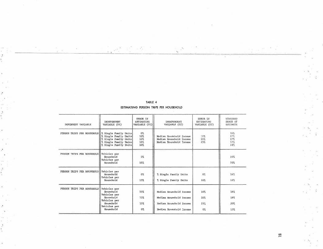
Assuming that the error in estimating the dependent variable of vehicles per house­hold is ±15 percent (with the errors in estimating density and income previously des­cribed), then the use of either (a) vehicles per household as a sole determinant, or (b) the linear combination of vehicles and income, yields (approximately) the same stan­dard error of estimate in estimating person trips per household (20%). A perturbation of a ±15 percent error in median household income (as a sole independent variable) causes the error in estimating person trips to rise from 15 percent to 20 percent (when compared to the theoretical case of vehicles estimated without any error, i.e., for known values of vehicles). See Table 4, Appendix, for a complete description of the results.

• •• *'

·.

44

60

y• 2.1ax0.656

50 • , • ~ 15'1!. ....... ...... ... 40

~ u c ~ .. .. 30 0 '; c

20

10

0 10 20 30 40 50 60 70 80 90 100

Hou11holds ptr Act1

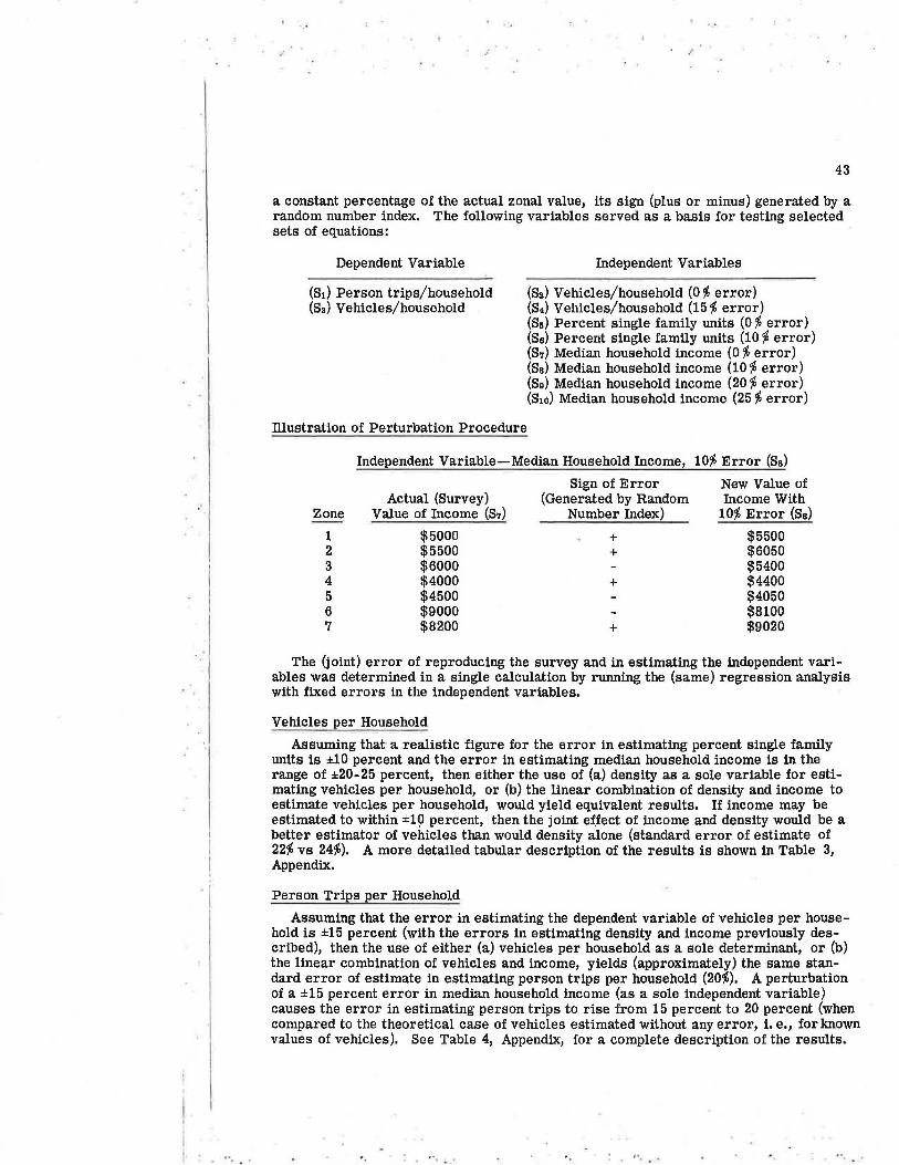
Figure 2. Relation between autos per acre and households per acre for 77 districts in Chicago, 1956-1957.

The joint error incurred in estimating the independent variables and reproducing the survey data (for the dependent variables) does not in itself yield a single clear-cut choice of trip generation equation (or procedure). It does narrow the list of variables and equations, however, to a few which now must undergo the test of forecasting efficiency.

USE AS A PREDICTIVE DEVICE

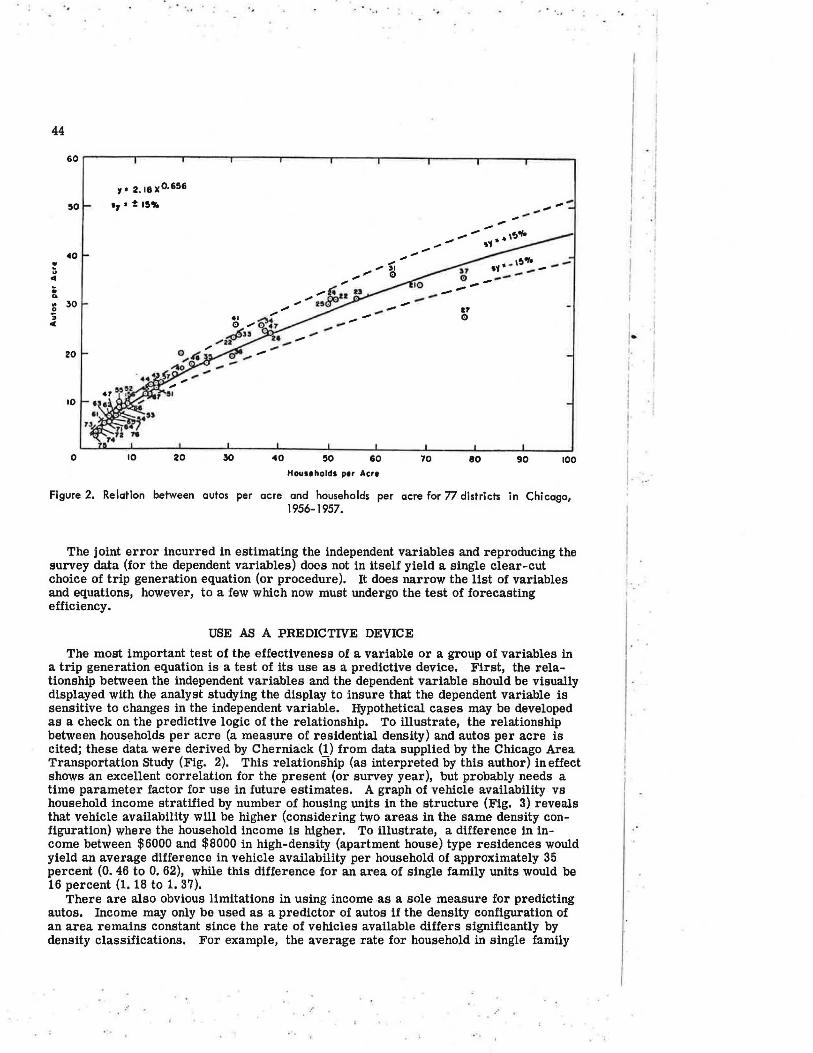
The most important test of the effectiveness of a variable or a group of variables in a trip generation equation is a test of its use as a predictive device. First, the rela­tionship between the independent variables and the dependent variable should be visually displayed with the analyst studying the display to insure that the dependent variable is sensitive to changes in the independent variable. Hypothetical cases may be developed as a check on the predictive logic of the relationship. To illustrate, the relationship between households per acre (a measure of residential density) and autos per acre is cited; these data were derived by Cherniack (1) from data supplied by the Chicago Area Transportation Study (Fig. 2). This relationship (as interpreted by this author) ineffect shows an excellent correlation for the present (or survey year), but probably needs a time parameter factor for use in future estimates. A graph of vehicle availability vs household income stratified by number of housing units in the structure (Fig. 3) reveals that vehicle availability will be higher (considering two areas in the same density con­figuration) where the household income is higher. To illustrate, a difference in in­come between $6000 and $8000 in high-density (apartment house) type residences would yield an average difference in vehicle availability per household of approximately 35 percent (0. 46 to O. 62), while this difference for an area of single family units would be 16 percent (1. 18 to 1. 37).

There are also obvious limitations in using income as a sole measure for predicting autos. Income may only be used as a predictor of autos if the density configuration of an area remains constant since the rate of vehicles available differs significantly by density classifications. For example, the average rate for household in single family

...

...

·.

1. I,

I

I.

I I

I I I I· I

.. -

DATA SOURCE PREL l_M I NARY HOME

INTERVIEW FINDINGS TRI-STATE TRANSPORTATION

COMMISSION 1963-1964

HOUSEHOLD INCOME 1000)

45

Figure 3. Vehicleavailabilityvs household income, stratified bynumberof housing units in the structure.

units earning $10, 000 per year is more than twice as great as the households living in 5 or more units per structure (ap~rtment houses) and earning a similar income.

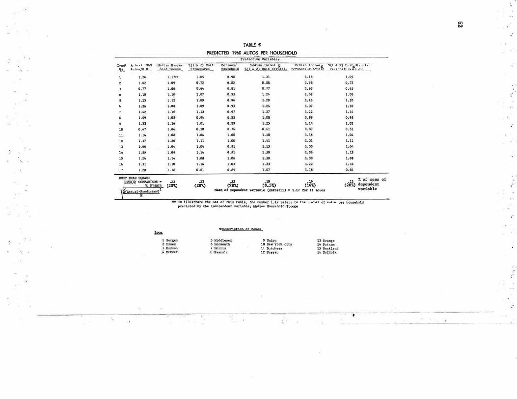
In order to derive an objective figure of merit for the effectiveness of the independent variables in predicting the dependent variable, the trip generation equation had to be tested over two points in time. To accomplish this for the dependent variable autos per household, auto registration data were abstracted from state vehicular records with census data describing the density and income variables. The base years for this analy­sis were 1950 and 1960, with counties in the New York Metropolitan Area as the geo­graphic area (or zones) used. This geographic detail is much too coarse but, because auto ownership rates were not available from the 1.950 census, county totals from auto registrations were the best available source. In the future (as in 1960), the census will report autos available to households on the census tract level such that a similar test of the predictive power of the independent variable may be conducted on a fine-grained geographic level.

The strategy involved in this analysis of evaluating the predictive power of the vari­ables for forecasting autos included deriving the best-fit linear regression line for 1950 for each of the independent variables and selected combinations of variables. These relationships were then used to estimate autos per household for 1960, and compared to the known actual figure of autos per household for 1960. The root-mean-square error was chosen as the figure of merit for comparing the results, which are shown in Table 5 in the Appendix.

TOT AL ERROR-BASIS FOR SELECTING THE TRIP GENERATION EQUATION

The procedure for calculating the total error of estimate for forecasting the depen­dent variable vehicles per household is illustrated below. It must be remembered that the joint error of reproducing the survey and error of estimating the independent

"• , ..

;

46

variables was derived from a zonal scheme of 278 zones while the error in predictive power was based on a coarse zonal scheme of only 17 zones. The total error of esti­mate, therefore, should not be used as an absolute value but as a figure of merit to compare the various trip generation equations.

Dependent Variable-Vehicles per Household

E1 Error in Reproducing E2 Survey (e1) and Error Error in

in Estimating Use as JE12 + E22

Independent Independent Variables (e2) Predictive Total Equation Variables Used (E1 = e1 + e2) Device Error

1 Percent single family units 24% 20.0% 31.0%

2 Percent single family units and median household income 23% 8.5% 24.5%

3 Median household income 49% 20.0% 53.0%

The results indicate that the linear combination of median household income and per­cent single family units yields a s ignificantly lower error of estimate (and is thus the recommended procedure) for forecasting vehicles per household when compared to the next best two equations. (It should be noted that for this sample analysis, percent single family units was given a± 10 % error and median household income a ±20% error of estimation. )

Unfortunately, data on person trips per household for two points in time were not yet available so that a similar analysis of the "total" forecast error could not be made for this dependent variable.

CONCLUSION

It is the purpose of this paper to present a methodology (or philosophy) to objectively select those independent variables that yield the best prediction of the dependent vari­ables of vehicles and person trips per household. The procedure has been illustrated by sample calculations, using the Tri-State Transportation home interview survey as the primary data source. In the near future, Census Bureau publications will describe the number of vehicles available to the households on a small-area basis along with measures of income and chlnsity. This rich source of data will make it possible to use a single consistent zonal scheme in calculating the three different sources of errors described in this paper in forecasting vehicles per household. It may also be possible to make similar calculations for the dependent variable of person trips per household if the original home interview surveys are updated so that household trip information is available for two periods of time.

In the next decade, many of tlie large metropolitan transportation studies will re­evaluate the travel demands to be generated by the households, update their travel sur­veys, and adjust their forecasts. It seems imperative to develop ~ criterion that ob­jectively tests and reevaluates the forecasting procedures to select that one which will most effectively describe the future. It is hoped that this paper stimulates more thought in this area of concern for transportation planners.

REFERENCE

1. Cherniack, Nathan. Critique of Home-Interview Type 0-D Surveys in Urban Areas. HRB Bull. 253, pp. 166-188, 1960 .

. ;

·.

-·---~-:----

Appendix

TABLE l

REGRESSION LINES-DEPENDENT VARIABLE, PERSON TRIPS PER HOUSEHOLD

E- R ql;'-a lndeoendent Variable(s) (Coefficient tl.O

~f!.d~M Variabl• 1•n No. D~scri-ption Ecuation of Conelat 1on)

X2 Total Vehicles/H, H. x1 c 4. 784X2 + 1.578 0.94

(X1) Pepon Trips/ 01 H.H, (X1=5.37) ~;r~~IJ! ~ uyears & x1 c 3. 978x3 - 5, 668 0. 72

n? :n Median Household Xi ~ 0. 0008156X

4 -0 . 06941 0,68

n> x4 Tlnllars Gross Density (living

04 XS Quarters/Sq, Mile) Xi a-Q,000099X5+ 6.736

0.68

Percent Single Unit x1 c 0.06597JCo + 3 . 292 05 X6 Structarea 0.93

06 X7 Log l;ros s !>ens ity x1 c-2.938X7 + 16,318 0,88

.· X2 Toto!. Vehicles/H. H. X1 c 4.205Xz + 0,9567X3

X3 'Persons 5 years & 0.95

07 Older -0.6180

A.< ·i;otal ve11:i.c1esfH. H.

X3 Person• 5 years & X1 = 3,502X2 + l.227X3 0.95 Older/H. H. + 0. 0001845X4 - 2. 042

08 X4 Median Dollars/H.H.

X2 Toul Vehicles/ll. H. Xi - 3.200Xi + l.200X:J X3 Pers011S 5 years ~· Older /ll. R. +0.0001955X[,. - 0.2040X7 0,95

X4 Median Dollar• 09 Household -1.040

'JO ... - ·- .., _ ___ n.n. .... .f~

X2 Total Vehicles/H.H. X1 • 2. 057X2 + 1. 012X3 X3 Persons 5 years. &

Older/H.H. + o.000111Xl,.+ o,02396xt; X4 Median Household 0,96 Dollars -1.007

X6. Percent Single Unit 10 Structure&

X3 Persona S years & Xl = 0.9217X3 + 0,05802Xo Older/H. H.

X6 Percent Single Unit + o. 985 0,93

11 Structures

s Std. Error of E!:timate

0.83

i. 67

1.74

1. 75

0 . 90

1.15

'l ,:77

0 . 73

0.73

0,67

0.85

sn.. ( <::<pressed in Percent

157.

llY.

"32'1.

337.

17'7,

21'1.

147.

147.

147.

127.

167.

IP­~

'·

· ..

' ·

...

Table l (Continued)

.· E· ~va •o Inde endent Variable(&)

··• Denende nt Variable No No. Descrintion Eauation

(X) Person Trips/H. H. X2 Total Vehicles/H. H. Xl a 2.854Xz + 0.0290Xi; 12 t 2.195

(Xl = 5.37) X6 Per Cent Single Unit

Structures

X2 Total Vehicle;/H.H. X1 • 4,50X2 • 0,20503.X7 v Log Gross Density + 2.570

13

X2 Total Vehicles/H. H. X1 m 4.501X2 + 0.000097Jl4 14 Median Household X4 Dollars +1.156

X2 Total Vehicles/a.a. x1 - s.011x2 + o.ooooo9x5 15 X5 Gross Den~ity(Living Qtrs/(mi) ) + 1.2725

16 X4 Median Household Dol- Xi • 0,000205X4 + 0.0583X

6 la rs X6 '7. Single Unit Structu1 os - 2-157

X4 ¥:dian Household Dol- ~l - o. 000358l14 - 2. 3966ll:7 rs

17 v Log Gross Density ,, + 11.909

X3 Persons ) years and X1 • l,267X3 +0.000272~ Older/H.H. + 0.0449Xt; • 1.374

18 X4 ~dian Household Dol-rs

X6 s<Mle Unit S ·- -X2 Total Vehicles/a.Ii:. Xl a 2~ 691X2 + O. 746X3 X3 Persons 5 yrs; & Olde1 19 H.H, +0,0246~ + 0.390 y~ .,., t"~no1 I"' n.;...r t- C: .. -.--.... ·-X2 Total Vehicles/a. H. X1 • 2,507X2 + 0,000107l14 X4 Median Household Dol-

20 lars. +0.0295~ + 1.74 X6 Percent Single Unit

" .• X3 l:iA~*~ (5 yrs. & 01- Xi • 3,1768~ + ,00063X4 21 X4 ~edian Household Dol- - 7 ,644 ars

~ i;oaal vehicMi'{~ · l!oi x1 = 4,1028Xz + 0, 000074~ 22 e ian Hous o -

la rs -0.3403~ + 2,887 X7 Log Gross Density

ll s (Coefficient Std. Error

of Correlation) of Estimate

0.95 • 75

0,94 .83

0.94 ,82

0,.94 .83

0.94 . 84

0.91 .98

0,95 . 74

0,95 .71

0.95 . 73

o.88 l.15

0.94 . 82

S/ 'J.., (Expreued in Per ceot)

14'7.

15% . 15'7.

15'7.

16'7.

187.

14'7.

13'7.

147.

21'7.

15'7.

11'>­(X)

.;.

..

..

...

TABLE 2

REGRESSION LINES-DEPENDENT VARIABLE, VEHICLES PER HOUSEHOLD

E- ll s sn. ~to Inde endent Variable(e} (Coefficient Std. Error (Exp-ressed

Deoendent Variable u - No. Descri,,tion Eouation of Correlation) of Estimatl!. in Pttcent)

Veh:!.cles/H.H. (li2) 23 X3 Persons 5 years &. X2 • 0, 7185X3 - 1.2009 0,66 0.35 45'}; Older/:I.H.

(x2

) = 0.79 Median Household Xi D 0.0001597Xt, - 0,2724 0.68 0.34 487. 24 X4 __ ,, ___

X5 Gross DeusitY" (Living X2 -·-0. 0000214X5 + 1. 089 o. 76 0.31 391. 25 "'·•-~--~·I <.o ><< \

26 X6 ~ Single Unit Xi • 0.01296X6 + 0.3843 0,93 0,17 22'%. '·

27 -0 Log Grose Density x2 • -0.60195Xr+ 3.0579 0,92 0,18 237.

X3 Persons 5 years & x2 • 0.5567X + OSJ001271X4 0.27 347. Older/H.H. 0.84 28 X4 Median Household -1.600 .· Dollars

X4 Median Household Dollars X:z • 0,00006141X4 • 0.515X. 0.95 0.15 19% 29 X7 Log Gross Density

+2.302

X3 Persons :S years & Xz - O,ll23X3 + o.000065JV.

30 Older/H, B.

0.95 0.14 18% X4 Medf:n Household - O. 4641X7 + 1. 780 Dol ar X7 Log GroH Density

X3 Persons 5 years & Xi • 0 .1236~ 0. 000046X4 Older/.H.H. 0.94 0.16 207. 31 X4 Median Household + o.0102x6 - o.178 Dollars

... X6 7. Single Unit

C!t-'C.1..-------

X4 Median Household Dol- Xi • O. 0000397X4 + O. Oll49X1 0.94 .16 20% 32 la rs X6 1.J!!!!~ll' Unit St'ruc- + 0.1663

X3 Per~• (~ yrs. & O~u- X:z • 0,065~ + O.Ol24X6 tl3

er H.B. 0.93 . 17 22%

X6 % Single Unit•Strucmt ~· + o. 221

.·

X3 Persbn• (5 years & x2

• 0.060X3

- 0.5833~ 0,93 .18 23~ Older) /H,H. 134 X7 Log Gross Denei ty + 2.800

~

'·

··.

DEPENDENT VARIABLE

VEIUCLES PER HOUSEHOLD

.,

VEHlCLES P£R HOUSEHO)Jl

·-

TABLE 3

ESTIMATING VEHICLES l'ER HOUSEHOLD

ERROR IN ERROR IN stA>~DARD WOl!l'ENDENT ESTIMAnNC IN DEPENDENT ESTIMATnfG ERROR OF

VARIABLE (01) VARI All LE ( 01) VARIABLE (02) VARIABLE (OZ) ESTnbl.TE

'%. Singl" Family Units 07. 227. 7. Si.ngle Family Units lO'Z Median ltousehold 1:ncorae 107. 22% 7. Single Family Units 101. Median llousehold Income 207. 237. 7. Single Family Units 107. Median l!ousehold Inc°""' 257. 23'Z Z Single Family Units Ot Median Household Income 07. 207. 7. Stngle Fami.ly Units 107. 247.

Median Household Income Ot 437.

Median Household tncomc 107. 46?:.

Median Household lncome 207. 497.

MedJ.an Household I.ncorce: 2!il 517:

- ·----·---.- .

en c

..

·-

TABLE 4

ESTIMATING PERSON TRIPS PER HOUSEHOLD

ERROR IN INDEPENDENT ESTDIATING INDEPENDENT

DEPENDENT VARIABLE VARIABLE (01) VARIABLE (01) VARIABLE (02)

PERSON TRIPS PER HOUSEHOLD % Single Family Units 0% % Single Family Units 10% Median Household Income % Single Family Units 10% Median Household Income % Single Family Units 10% Median Household Income % Single Family Uni ts 10%

PERSON TRIPS PER HOUSEHOLD Vehicles per Household 0%

Vehicles per Household 15%

PERSON TRIPS PER HOUSEHOLD Vehicles per Household 0% % Single Family Units

Vehic lea per Household 15% % Single Family Units

PERSON TRIPS PER HOUSEHOLD Vehicles per Household 15% Median Household Income

Vehicles per Household 15% Median Household Income

Vehicles per Household 15% Median Household Income .. Vehicles per Household 0% Median Household Income

ERROR IN ESTIMATING

VARIABLE (02)

107, 20% 25%

0%

10%

10%

20%

257,

0%

STANDARD ERROR OF ESTIMATE

16% 177. 17% 17% 187.

16%

20%

14%

16%

19%

19%

20%

15%

C1I .......

· ..

· ..

'·

· ..

··.

...

.,

TABLE 5

PREDICTED 1960 AUTOS PER HOUSEHOLD Pra.di.cc.l vc Varlablc.a

Zone" Act.u:,l 1960 ~d!.110 H~-::c:· :f(I 5 2j Ublt Pouons/ M:edUa tnc:ome & 1'~;::!:1n:::A ~(1 & 2) t'ri.i~_truc,ts.

...!9.:. AtJtos/R.'H 1 hold l~!!t!"la SC.rw::t'Uras l\r;iu!l' ahold ,;p & 2.) Uolt Scruc.u . tter,-011:11 /l!ous old

1.26 l.l:IH- 1.05 0.90 l .J I 1. 16 l.O>

1.02 1.09 O.IZ 0.82 o.~ 0.95 O. IJ

o;n 1.06 0 • ...,. 0.81 0 . 77 0.93 ·0.6S

1.18 1.10 1.07 o.u 1.2• l.09 1.oa

S. LZJ 1.u 1.09 0 . 96 1.29 1.16 1.10

1.26 1.08 l.09 0 . 93 1. 24 1.01 l.10

1.42 1.16 1 •. u 0.'1 1.37 l.ll 1.14

1.09 L.08· 0.94 o.ss I.OS 0 . 99 0.95

9 1.33 l.16 1.01 0.89 1.2.S t.14 1.02

10 0 . 47 1.06 o.so 0 . 76 0.61 0.87 O.SI

11 1.14 l.08 1.04 I.DO 1.18 1.16 1.04

12 1. l1 1.20 1.11 1. 00 l.41 I.JI 1.11

13 1.06 1.04 \.04 0.91 l.LJ 1.00 1.04

14 I. 59 1.09 1.14 0.91 1.30 1.06 l.15

15 1.24 1.1• 1.08 l.06 1.30 1 . 30 i.oa tu 1.n \.10 1.16 1.03 1.33 l.22 1.16·

17 l.20 l.18 0 . 81 0.89 1.07 1.16 0.81

IUX)T - SQl)ARE 23

1. o.f mean of ER!IOR COMPAi.ISON • .23 .23 .33 .10 .19

(8.51.) (161.) ( 2'07..) depend.ent (207:) (201.) (281.) Mean of Dependent Varioble (.latoafBB) • 1.17 for 17 zooea vad•b l e

** To tllun:r;ate the wie of thh ubh, chir: aumbe.c 1-. t7 re.fec.e to the~ o! au.cm per h.a'i:u:ebold p rGt..cccd by th• !.nda·pie:ndc_at varbblc. . Hedia1;1 Hoi,ta:ehold llicome

!!m!,,

le rs en 1 Ene:iit l Hudson ). Me-.rce r-

*'Pe,.er.beicr:\ of totl.H

S M!ddlou 6 tit:oom:outh 7 )ior'rh $ 'PllH.ll!c

9 Dnto·n 10 Reu vo·~.c. Ci cy 11 Du t:ch.e-u 12. N•H•U

L3 0 C"•u.fl• 14 Putn.a. lS Rcck:hnd l6 Suffolk

------- - . -- -

~

.·