Solving the Master Linear Program in Column Generation

Algorithms for Airline Crew Scheduling using a Subgradient

Method

Per Sjogren

November 28, 2009

Abstract

A subgradient method for solving large linear programs is implemented and analyzed ina column generation framework. A performance comparison of the implementation ismade versus the commercial linear programming solver XPress. Computational resultsfrom tests using data from airline crew scheduling, in particular crew rostering, showthat the method performs very well in a column generation scheme, compared to bothsimplex and barrier methods.

Acknowledgements

I would like to express thanks to Curt Hjorring and Ann-Brith Stromberg, my supervi-sors at Jeppesen Systems AB and Goteborgs universitet, respectively. Thanks also goto Tomas Gustafsson, Mattias Gronkvist, Andreas Westerlund, and the other membersof the optimization group at Jeppesen who made this thesis possible.

1

Contents

1 Introduction 3

2 Preliminaries 5

2.1 Lagrangian Duality . . . . . . . . . . . . . . . . . . . . . . . . . . . . . . 52.2 Optimality conditions . . . . . . . . . . . . . . . . . . . . . . . . . . . . 62.3 Subgradients of the Lagrangian dual function . . . . . . . . . . . . . . . 7

3 Crew Rostering 8

3.1 The basic model . . . . . . . . . . . . . . . . . . . . . . . . . . . . . . . 83.2 Extending the model . . . . . . . . . . . . . . . . . . . . . . . . . . . . . 93.3 Soft constraints . . . . . . . . . . . . . . . . . . . . . . . . . . . . . . . . 103.4 Solving Rostering Problems . . . . . . . . . . . . . . . . . . . . . . . . . 11

4 Column Generation 12

4.1 Dantzig-Wolfe decomposition . . . . . . . . . . . . . . . . . . . . . . . . 124.2 General column generation . . . . . . . . . . . . . . . . . . . . . . . . . 13

5 An overview of methods for solving linear programs 16

5.1 The Simplex Method and Variations . . . . . . . . . . . . . . . . . . . . 165.2 Barrier Methods . . . . . . . . . . . . . . . . . . . . . . . . . . . . . . . 175.3 Subgradient Methods . . . . . . . . . . . . . . . . . . . . . . . . . . . . . 19

5.3.1 Inequality constraints and restricting the dual space . . . . . . . 205.3.2 Deflected Subgradients . . . . . . . . . . . . . . . . . . . . . . . . 225.3.3 Variable Target Value Methods . . . . . . . . . . . . . . . . . . . 22

6 Computational Tests and Results 24

6.1 The Algorithm . . . . . . . . . . . . . . . . . . . . . . . . . . . . . . . . 246.2 Test cases . . . . . . . . . . . . . . . . . . . . . . . . . . . . . . . . . . . 256.3 Comparison with XPress . . . . . . . . . . . . . . . . . . . . . . . . . . . 266.4 Results within column generation . . . . . . . . . . . . . . . . . . . . . . 27

7 Conclusions 36

2

Chapter 1

Introduction

For an airline company crew salaries and costs constitute the second largest cost nextto fuel. Cost-efficient crew scheduling is thus vital for the survival of a company andvarious optimization models and methods for minimizing personnel costs have been usedfor a long time.

As an example, one approach to select schedules for crew would be to enumerateall possible schedules during the duty period for each crew member and associate acertain cost to each schedule. Then it would in principle be possible to choose thecheapest combination of schedules such that every task is scheduled to an employee.However, such an approach is not practically possible due to the huge number of possibleschedules. Instead a generation technique called column generation may be used [5].Columns (which in this case represent schedules) are then generated as needed.

One part of the column generation process is solving linear programs (LP). Althougheffective means to solve linear programs exist, e.g. the simplex and the dual simplexmethods, these methods possess an exponential worst case complexity ([9] pp. 434–435). In addition, the solutions produced by the simplex method are in several casesinefficient for the column generation process and approximate (different) solutions mightbe preferrable [8].

Due to the complexity of scheduling optimization problems many airline companiesuse optimization products developed by Jeppesen Systems AB to manage their crewscheduling. The optimization process of large-scale scheduling problems at Jeppesenincorporate many different optimization techniques of which column generation is one.The reason for this study is that it was noted at Jeppesen that a large amount of thecolumn generator runtime was spent in the linear programming solver XPress. It wasargued that a more specialized solver might be able to solve the linear programs faster.Also, as mentioned above, using a different solution technique rather than the simplexmethod for the linear program may accelerate the convergence in the column generationprocess.

In this thesis a subgradient method with variations is described and computationalresults using this method, both on pure LPs and in a column generation framework, ispresented. Most of the development made in this thesis is based on work by Sherali andcoauthors [7, 11, 12].

The outline of this thesis is as follows. In the next chapter the mathematical back-ground in optimization theory used in the thesis is presented. In Chapter 3 the crewscheduling process and modelling is described. Chapter 4 contains a brief outline ofcolumn generation. Different solution methods for linear programs are presented in

3

Chapter 5. Chapter 6 presents computational results and conclusions are drawn inChapter 7.

4

Chapter 2

Preliminaries

In this chapter a few basic results in optimization theory is presented and most of thenotation used in the thesis is introduced. Lagrangian duality is needed for explainingthe role of solving linear programs within column generation. Section 5.1 briefly touchesLP duality, for which Lagrangian duality is also needed. Subgradients are introduced inSection 2.3 and used in the subgradient methods presented in Section 5.3. Optimalityconditions are presented and used in Sections 5.1 and 5.2, respectively.

Lower-case bold letters used as variables or constants, e.g. x, b and µ denote realcolumn vectors. Either the context will limit the size of the vectors or their dimen-sions will be given. Likewise 0 denotes the zero-vector and 1 denotes a vector of ones.Functions may be vector-valued, e.g. h : R

n → Rm, and are then also written in bold.

The letteres A and D denote matrices, L denotes the Lagrangian function as defined inSection 2.1 and other capital letters denote vector spaces.

If b and c are two vectors, then b ≥ c is true if their elements bi ≥ ci for all i. Otherrelations, for example x = b, x ≤ b, are defined analogously. Thus x ≥ 0 is true if allcomponents of x are non-negative.

For a minimization problem

minimize f(x), (2.1a)

subject to h(x) = b, (2.1b)

g(x) ≤ 0, (2.1c)

x ∈ X, (2.1d)

where h : Rn → R

m,b ∈ Rm,g : R

n → Rk, f : R

n → R and X ⊆ Rn. If the optimal

objective value exists, we denote it by f∗, which is then attained at some feasible pointx∗. A point x ∈ R

n is said to be feasible in (2.1) if h(x) = b, g(x) ≤ 0 and x ∈ X.

2.1 Lagrangian Duality

The general optimization problem (2.1) can be very hard to solve depending on theproperties of f, g, h and X. Various relaxation techniques can be used to produce anapproximate solution, for example by extending the set X or removing a few of theconstraints. One such technique is the Lagrangian relaxation. See [13] Ch. 2 for adefinition of relaxation in an optimization context.

Consider the general optimization problem (2.1) where we assume that the inequalityconstraints (2.1c) are absent, i.e., k = 0. Instead of requiring the constraints (2.1b) to

5

be fulfilled we introduce a cost in the objective function for breaking these constraints.Define the Lagrangian function

L(x, µ) = f(x) + µT (b − h(x)), x ∈ Rn, µ ∈ R

m,

and the Lagrangian dual function

θ(µ) = minx∈X

L(x, µ), µ ∈ Rm. (2.2)

If x solves (2.2) and x∗ solves (2.1), then the relations

θ(µ) = f(x) + µT (b − h(x)) ≤ f(x∗) + µT (b − h(x∗)) = f(x∗) = f∗ (2.3)

hold, since x minimizes L(x, µ) over x ∈ X. Thus for every µ ∈ Rm, θ(µ) is a lower

bound on the optimal value f∗. To get the highest possible lower bound we solve theLagrangian dual problem to

θ∗ = maxµ∈Rm

θ(µ). (2.4)

From the above follows that θ∗ ≤ f∗. We define Γ = f∗ − θ∗ as the duality gapfor the problem (2.1) with k = 0. Also, for any feasible point x ∈ {x ∈ X |h(x) = b},f(x) is an upper bound on the primal optimal value f∗. If we know that Γ = 0 (whichholds, e.g. for linear programs) and the dual problem is solved to optimality we caneasily check how good a feasible point is by comparing its objective value with the lowerbound.

The Lagrangian dual function has some nice properties as, e.g. concavity.

Proposition 2.1.1. The dual function θ is concave.

Proof. Let µ0, µ1 ∈ Rm and 0 ≤ α ≤ 1. It then holds that

θ(αµ0 + (1 − α)µ1) = minx∈X

(

f(x) + [αµ0 + (1 − α)µ1]T [b − h(x)]

)

= minx∈X

[

α(

f(x) + µT0 [b − h(x)]

)

+ (1 − α)(

f(x) + µT1 [b − h(x)]

)]

≥ α minx∈X

(

f(x) + µT0 [b − h(x)]

)

+ (1 − α) minx∈X

(

f(x) + µT1 [b − h(x)]

)

= αθ(µ0) + (1 − α)θ(µ1).

The result follows.

This means that the Lagrangian properties are not dependent on the possible convex-ity of f . The Lagrangian dual function is, however, non-differentiable and an ordinaryNewton method can not be used to solve the Lagrangian dual problem. For example asubgradient method can be used instead, see Chapter 5.

2.2 Optimality conditions

The Karush-Kuhn-Tucker (KKT) optimality conditions constitute a very useful tool forboth confirming optimality and designing optimization methods. The KKT optimalityconditions are stated without a proof for a special case as needed in this thesis; for amore thorough and general presentation, see for example the textbook [1], Ch. 5.

6

Consider the minimization program (2.1), where we assume that X = Rn. Assume

further that the functions f and g are convex and differentiable and that the functionsh are linear. Then a feasible point x ∈ R

n is optimal in (2.1) if and only if there existvectors µ ∈ R

m and λ ∈ Rk such that

k∑

i=1

λi∇gi(x) +m

∑

i=1

µi∇hi(x) + ∇f(x) = 0, (2.5a)

λigi(x) = 0, i = 1, . . . k, (2.5b)

λ ≥ 0. (2.5c)

Now consider the problem (2.1); the conditions in (2.5) are then simplified. ForLagrangian duality a primal-dual pair (x∗, µ∗) is optimal in (2.1) — as in Section 2.1assuming that the inequality constraints (2.1c) are absent (i.e., k = 0) — if x∗ is feasibleand

x∗ ∈ arg minx∈X

L(x, µ∗).

This follows from the inequality (2.3) and the fact that L(x∗, µ∗) = f(x∗) for feasiblex∗. If k > 0, i.e. the program contains inequality constraints, the Lagrangian functionis defined slightly differently and an additional condition analogous to (2.5b) is neededto ensure that L(x∗, µ∗) = f(x∗) for all feasible x∗. Again, see for example [1] for athorough presentation of optimality conditions.

2.3 Subgradients of the Lagrangian dual function

Let the function θ : Rm → R be concave on R

m. A subgradient to θ at µ0 is a vectorλ ∈ R

m such that for all µ ∈ Rm it holds that

θ(µ) ≤ θ(µ0) + λT (µ − µ0). (2.6)

The subdifferential of θ at µ0 is the set of all subgradients at this point and is denotedby ∂θ(µ0). If the subdifferential of θ at µ0 contains the 0-vector then µ0 is a maximizerof θ [1, p. 159]. The function θ is differentiable at µ0 if the subdifferential contains onlya single element which then equals the gradient of θ at µ0.

Consider the Lagrangian dual function θ : Rm → R. As shown in the proof of

Proposition 2.1.1 this function is concave. Let x0 ∈ arg minx∈X L(x, µ0), i.e., x0 solvesthe program (2.2). Then b − h(x0) is a subgradient to θ at µ0 since, for all x ∈arg minx∈X L(x, µ),

θ(µ) = f(x) + µT (b − h(x)) ≤ f(x0) + µT (b − h(x0)),

and sinceθ(µ0) = f(x0) + µT

0 (b − h(x0)),

this implies thatθ(µ) − θ(µ0) ≤ (b − h(x0))

T (µ − µ0).

In this thesis subgradients will mostly be considered with respect to Lagrangian dualfunctions. We may define subgradients for convex functions analogously; the inequalityin (2.6) is then reversed.

7

Chapter 3

Crew Rostering

In this chapter a brief outline of modelling rostering problems is given and in its last sec-tion a solution process is presented. In the rostering process a set of activities consistingof pairings (i.e. sequences of flights for a duty period), reserves, training activities, andvarious ground duties need to be covered by the available crew. All these activities arereferred to as tasks. A collection of tasks for a specific crew member is called a roster.

There are numerous of rules and regulations that the personal rosters must follow.In this thesis we will limit the description of modelling by presenting examples of rulesand how to model them and refer the reader to [5] for a more detailed explanation.

In the following subsection the basic rostering model is presented. Section 3.2 ex-tends the model by introducing a few example constraints. Soft and hard constraintsare presented in Section 3.3 and in Section 3.4 a brief solution process is outlined.

3.1 The basic model

The rostering problem is built by a set T of tasks and a set C of crew members. Foreach crew member k ∈ C we need to assign a legal roster Rjk

⊂ T such that

T = Rj1 ∪ Rj2 ∪ · · · ∪ Rj|C|,

where Rji∩ Rjk

= ∅ if i 6= k. This ensures that each task is assigned to exactly onecrew member. Additionally, this set of rosters should be the ‘best’ choice in some sense.What ‘best’ means is often a combination of, e.g. paid overtime, a fair distribution ofattractive rosters, and quality of life for crew members.

In order to formulate the rostering problem as an optimization problem we modela roster Ri as a binary column vector ai such that aji = 1 if column i is a roster forcrew member j ∈ {1, . . . , |C|}. For each task j that the roster includes a(j+|C|)i, j ∈ T .All other aji = 0. Let then xi be a binary decision variable denoting whether to usethe roster modelled by ai or not. Let also ci be the cost associated to the roster Ri.Finally we define the matrix A = [a1 . . .ak] ∈ {0, 1}m×n, where n is the total number ofpossible rosters and m = |C|+ |T | is the sum of the number of tasks and crew members.

The first |C| rows of A make sure that every crew member gets assigned to exactlyone roster; these are called assignment constraints. The second block of A, called activityconstraints, makes sure that every task gets assigned exactly once. This is illustratedin Table 3.1.

8

The matrix A rel rhs DescriptionCrew 1 Crew 2 . . . Crew |C|

R1 R2 R3 R4 R5 R6 . . . Rn−2 Rn−1 Rn

1 1 1 0 0 0 . . . 0 0 0 = 1 Assignment0 0 0 1 1 1 . . . 0 0 0 = 1 constraints

. . ....

...0 0 0 0 0 0 . . . 1 1 1 = 11 1 0 0 1 0 . . . 1 0 0 = 1 Activity0 1 1 0 0 1 . . . 0 1 0 = 1 constraints...

......

......

......

......

......

1 0 1 1 0 0 . . . 0 0 1 = 1

Table 3.1: The matrix A, relations (rel), and right-hand sides (rhs) for the basic rosteringmodel; here three different rosters are generated for each crew member.

From the above we conclude that in its simplest form the rostering problem is aset-partitioning problem (SPP), that is, to

minimizex

cTx, (3.1a)

subject to Ax = 1, (3.1b)

x ∈ {0, 1}n, (3.1c)

where c ∈ Rn and A ∈ {0, 1}m×n.

One intuitive solution approach to the rostering problem would be to generate allpossible rosters Rj , j ∈ J , that is, to form all possible subsets of T and pick the bestones. This corresponds to generating the full matrix A and solving the problem (3.1).However, this approach fails at first glance because of the huge number of possiblerosters for practical instances.

Alternatively one can generate a large number of rosters and solve a set-partitioningproblem in order to obtain the best solution consisting of combinations of the rostersgenerated. Depending on the solution characteristics more rosters (columns) can be gen-erated until the solution is close to optimal. This process, known as column generation,is explained in Chapter 5.

3.2 Extending the model

The basic rostering model can be extended in several ways to include more complicatedrules. If more than one crew member is needed for a specific task — for example,a certain training activity may need two captains — the right-hand side of the rowrepresenting that task is simply changed from 1 to the required number. For every taskrequiring an additional qualification a constraint row is added. One example of such aqualification is that a flight between two different countries may need at least one crewmember to speak an additional language. Table 3.2 illustrates this.

When a task requires more than one crew member it is preferrable that not onlyinexperienced crew are assigned to it. How to model this is illustrated in Table 3.3. If,for some reason, two crew members can not work together this is modelled analogously.

9

The matrix A rel rhs DescriptionCrew 1 Crew 2 . . . Crew |C|

R1 R2 R3 R4 R5 R6 . . . Rn−2 Rn−1 Rn

1 1 1 . . . = 1 Assignment1 1 1 . . . = 1 constraints

. . ....

.... . . 1 1 1 = 1

1 1 0 0 1 0 . . . 1 0 0 = 2 Task 10 0 0 0 1 0 . . . 0 0 0 ≥ 1 T. 1, language0 1 1 0 0 1 . . . 0 1 0 = 2 Task 20 0 0 0 0 1 . . . 0 0 0 ≥ 1 T. 2, language1 0 1 1 0 0 . . . 0 0 1 = 3 Task 30 0 0 0 0 0 . . . 0 0 1 ≥ 1 T. 3, language

Table 3.2: An extended rostering model including language requirement constraints.Crew member 2 knows the language required for Tasks 1 and 2 but not for task 3. Crewmember |C| knows the language required for Task 3.

The matrix A rel rhs DescriptionCrew 1 Crew 2 . . . Crew |C|

R1 R2 R3 R4 R5 R6 . . . Rn−2 Rn−1 Rn

1 1 1 . . . = 1 Assignment1 1 1 . . . = 1 constraints

. . ....

.... . . 1 1 1 = 1

1 1 0 0 1 0 . . . 1 0 0 = 2 Task 11 1 0 0 1 0 . . . 0 0 0 ≤ 1 T. 1, inexperience0 1 1 0 0 1 . . . 0 1 0 = 2 Task 20 0 0 0 0 1 . . . 0 0 0 ≤ 1 T. 2, Inexperience1 0 1 1 0 0 . . . 0 0 1 = 3 Task 30 0 0 0 0 0 . . . 0 0 0 ≤ 1 T. 3, Inexperience

Table 3.3: An extended rostering model including inexperience constraints. Crew mem-ber 1 is inexperienced for Task 1, crew member 2 is inexperienced for Tasks 1 and 2.

The difference is that crew members might be inexperienced for one task but not foranother, while incompatibility between two crew members holds for all tasks.

3.3 Soft constraints

When using optimization software for creating a schedule the answer “This problemis infeasible” is seldom an acceptable outcome. What the user wants to know whenthe problem is infeasible is whether he or she can solve the scheduling problem by,for example, calling in extra staff or paying workers for over-time. For this reason apartition is often made between hard and soft constraints. Hard constraints may notbe broken at all, while soft constraints may be broken at a cost.

10

Consider the problem to

minimizex

cTx,

subject to Ax = b, (3.2a)

Dx ≤ d, (3.2b)

x ∈ [0, 1]n. (3.2c)

Let us assume that the constraints (3.2a) are soft in the sense that a solution x suchthat Ax ≤ b is allowed and that the constraints (3.2b) may be broken. For this settingwe introduce the variables s and t along with costs for breaking each of the constraintsand formulate the problem with soft constraints as that to

minimize cTs s + cT

t t + cTx, (3.3a)

subject to s + Ax = b, (3.3b)

−t + Dx ≤ d, (3.3c)

x ∈ [0, 1]n, (3.3d)

s, t ≥ 0. (3.3e)

The values of variables s and t denote how much the rules modelled are broken.Decisions must then be made on whether or not the constraints have been violated toomuch and whether the extra cost is acceptable.

3.4 Solving Rostering Problems

The size of rostering problems solved by Jeppesen software (or of any fairly large schedul-ing problem) makes a brute force solution approach impossible. Instead some sort ofheuristic generation process combined with fixing strategies may be used.

One approach is to put a lot of effort in generating good rosters. This could be donein a column generation scheme connected to some LP solver. When an LP-relaxationof the original problem has been solved, variables with values ‘close to 1’ can be fixedto 1 and the restricted problem is solved. This will iteratively generate a sequence ofsolutions which eventually approaches an integer solution.

Obviously a large number of LPs will have to be solved in this process. Thus it isessential that solving LPs is done as fast as possible. Column generation is explainedin the following chapter and various LP solvers are discussed in Chapter 5.

Another approach is to use local search to iteratively improve a solution. An initialfeasible assignment of all trips is then required. This can in most cases be done by asimple greedy algorithm since the initial assignment can disregard fairness and costs.

11

Chapter 4

Column Generation

In this chapter we consider the problem to

minimize cTx, (4.1a)

subject to Ax = b, (4.1b)

x ∈ X, (4.1c)

where the set X ⊂ Rn is defined by linear (in)equalities and possibly also integer

requirements. The general setting is that the matrix A has too many columns for theprogram (4.1) to be computationally tractable. Instead we generate columns of A asthey are needed. An example of this is the rostering problem, described in Chapter3, in which A consists of all possible rosters for all crew members. However, beforelooking at the general column generation scheme we present the classical Dantzig-Wolfedecomposition scheme for linear programs. For Dantzig-Wolfe decomposition, see forexample [6], and for column generation in general, see [8].

4.1 Dantzig-Wolfe decomposition

Consider the problem to

minimize cTx, (4.2a)

subject to Ax ≥ b, (4.2b)

Dx ≥ d, (4.2c)

x ≥ 0, (4.2d)

with optimal value z∗.We define the polyhedron P = {x ∈ R

n+ |Dx ≥ d} 6= ∅. If P is bounded then each

point in P can be expressed as a convex combination of its extreme points {pq}q∈Q. If Pis unbounded a nonnegative linear combination of its extreme rays need to be includedas well, but for simplicity we restrict our presentation to the case where P is bounded.1

Thus we can express

P =

x ∈ Rn

∣

∣

∣

∣

∣

∣

x =∑

q∈Q

pqλq,∑

q∈Q

λq = 1, λq ≥ 0, q ∈ Q

1The rostering problem introduced in the previous chapter has this property since the variables arecontinuously relaxed binary variables. That is, all feasible variable values are in the interval [0, 1].

12

and the problem (4.2) can be expressed as the so called (full) master problem to

minimize∑

q∈Q

λqcTpq, (4.3a)

subject to∑

q∈Q

λqApq ≥ b, (4.3b)

∑

q∈Q

λq = 1, (4.3c)

λq ≥ 0, q ∈ Q. (4.3d)

If only a subset Qi ⊂ Q of the extreme points is known the restricted master problem(RMP) is defined by substituting Q by Qi:

minimize∑

q∈Qi

λqcTpq, (4.4a)

subject to∑

q∈Qi

λqApq ≥ b, (4.4b)

∑

q∈Qi

λq = 1, (4.4c)

λq ≥ 0, q ∈ Qi. (4.4d)

Columns (i.e., extreme points of P ) of the restricted master problem are generated bysolving the subproblem

pi+1 ∈ arg min{(

cT − µTi A

)

x − vi |Dx ≥ d,x ≥ 0}

, (4.5)

with optimal value zi ≥ z∗, and where (µi, vi) is an optimal solution to the linear pro-gramming dual of the restricted master problem (4.4). Note that pi+1 is an extremepoint of P . Here, the dual variables µi and vi correspond to the constraints (4.4b) andthe convexity constraint (4.4c), respectively. Defining Qi+1 = Qi ∪ {pi+1}, we add the

column(

(Api+1)T , 1

)Twith cost coefficient cTpi+1 to the restricted master problem.

The restricted master problem is then solved again producing new dual variable values(µi+1, vi+1). The optimal value of (4.5) equals the reduced cost of the variable λi+1, andthe process is iterated until the optimal value of (4.5) is non-negative. The latter meansthat no columns are then added to the restricted master problem, since no column re-sults in an improvement. Thus, the solution to the final restricted master problem isalso a solution to the full master problem.

4.2 General column generation

In this section we consider a linear program in a standard formulation with the additionalconstraint that every variable has an upper bound. This bound is here set to 1 but mayvary between variables. Thus, let the following problem be the master problem, MP:

zMP = minimize cTx (4.6a)

subject to Ax = b, (4.6b)

x ∈ X ≡ [0, 1]n, (4.6c)

13

where A ∈ Rm×n and we assume that n ≫ m. Now, assuming that i columns of A

are known, we partition A into one known and one unknown part, i.e., A = [Ak, Au].Analogously we partition c = [cT

k , cTu ]T and x = [xT

k ,xTu ]T . This, with y = xk, allows

the formulation of the restricted master problem, RMP, as to

zRMP = minimize cTk y (4.7a)

subject to Aky = b, (4.7b)

y ∈ [0, 1]i. (4.7c)

The program (4.7) is a restriction of MP since, if y is feasible in (4.7) and x = (yT ,0T )T ,then x is feasible in (4.6). Since [0, 1]i × {0}n−i is a subset of X, it follows that zMP ≤zRMP. Relaxing the equality constraints (4.7b) in RMP (as in Section 2.1) we obtainthe Lagrangian function

Lk(y, µ) = cTk y + µT (b − Aky)

and the Lagrangian dual problem

maximizeµ∈Rm

θk(µ)

whereθk(µ) = µTb + minimize

y∈[0,1]i(cT

k − µT Ak)y.

Since MP and RMP have the same number of rows and the columns of Ak is a subsetof those of A, a dual vector µ for RMP is also a dual vector for MP and it can be usedto obtain information about MP.

Let µ be any Lagrangian dual vector (for example obtained by solving the La-grangian dual to RMP approximately). Then, if the reduced costs cu − µT Au are allnon-negative the corresponding variables xu in MP will be set to 0 and

θk(µ) = θ(µ) = µT b + maxx∈[0,1]n

(cT − µT A)x

is a lower bound on zMP. If further (y, µ) is an optimal Lagrangian primal-dual solutionfor RMP then the Langrangian duality optimality conditions from Section 2.2 yields that((yT ,0)T , µ) is an optimal primal-dual solution to MP.

However, if the reduced cost for some variable in xu is negative, then θ(µ) < θk(µ)and θk(µ) is not necessarily a lower bound on zMP. We may then let the column cor-responding to the smallest reduced cost enter Ak and compute a new dual solution,possibly warm-starting the LP solver with the previous dual variable values. Alter-natively we may add the j columns with smallest (but still negative) reduced costs.Assuming that the goal is to produce a lower bound on zMP, this process will terminateeither when all columns in MP are generated or when the reduced costs correspondingto the unknown variables xu are all non-negative.

Whether this process is worthwile depends on the manner in which columns aregenerated and how the reduced costs are calculated. In a practical rostering problemthe total number of columns is often very large and calculating the reduced costs forall possible columns is not possible. Instead it is possible to heuristically generate a setof columns utilizing the dual vector and the (relatively well-known) structure of A. Ifwe do not manage to heuristically generate any columns with negative reduced costs

14

we may assume that the dual vector is close to optimal, depending on how well theheuristic solution approximates the optimal one.

As an example of a heuristic for generating columns with negative reduced cost, agraph can be generated to represent all the tasks. Arcs with a cost associated to themrepresent tasks. Solving a k-shortest path problem in the graph will then yield a columnwith low reduced cost. The correctness of this pricing heuristic is dependent on howwell the cost of arcs represent the actual cost of rosters.

15

Chapter 5

An overview of methods for

solving linear programs

The previous chapter presents the column generation principle and defines a sequenceof linear programs that need to be solved throughout the column generation procedure.The successive linear programs are similar to each other, thus the solution of a previouslysolved linear program may be utilized when solving the next one. This warm-start (whenpossible) often reduces runtime considerably. This chapter describes a few differentmethods for solving this sequence of linear programs.

We first give a brief description of the simplex method with variations for linearprogramming. In Section 5.2 barrier methods, such as the interior point method, isdescribed. The following sections are then focused on subgradient methods with varia-tions.

5.1 The Simplex Method and Variations

The simplex method is due to George Dantzig and revolutionized the field of optimiza-tion. Since it is a well-known method this section will contain a very brief outline of itand refer the reader to, for example, the textbooks [1] and [9] for details.

This section will consider a linear program in standard form, that is,

minimize cTx, (5.1a)

subject to Ax = b, (5.1b)

x ≥ 0, (5.1c)

where A ∈ Rm×n and we denote the feasible set by Q = {x ∈ R

n |Ax = b,x ≥ 0}.A linear program that has a solution also has a solution at an extreme point of

its feasible set ([1, p. 219]). In its simplest form the simplex method initiates at anextreme point of the polytope Q and moves along the edges of Q via extreme pointsuntil optimality is verified. Under non-degeneracy assumptions the simplex algorithmterminates after a finite number of steps since there is only finitely many extreme pointsof a polytope. While in many cases the simplex method is very efficient its worst-casecomplexity is very bad; see for example [9, pp. 434–435] for an example where everyextreme point of Q is visited before termination. This example results in an exponentialnumber of iterations.

16

A solution of RMP given by the simplex method, an extreme point of the feasi-ble set, is not the dual solution needed for column generation. However, the simplexmethod produces both primal and corresponding dual solutions. Lagrangian relaxingthe constraints (5.1b) (as in Chapter 2) results in the Lagrangian dual problem to

maximizeµ∈Rm

(

bT µ + minimizex≥0

(cT − µT A)x

)

. (5.2)

If a dual solution µ results in a negative reduced cost (c− µT A)i for any variable xi thecorresponding Lagrangian subproblem solution becomes unbounded. This dual variablevalue µ can then obviously not be optimal in the Lagrangian dual problem. Thus wecan restrict the dual problem by excluding dual variable values producing unboundedsubproblems. This restriction does not change the optimal value and gives an equivalentformulation of the Lagrangian dual problem, the linear programming dual to

maximize bT µ, (5.3a)

subject to AT µ ≤ c, (5.3b)

µ ∈ Rm. (5.3c)

The linear programming primal and dual problems are closely related. As mentionedin Section 2.1, the corresponding duality gap is zero. The KKT optimality conditionsfor a primal-dual pair (x, µ) may thus be expressed as

Ax = b, (5.4a)

AT µ ≤ c (5.4b)

xT (c − µT A) = 0, (5.4c)

x ≥ 0. (5.4d)

Thus x ∈ Q is optimal in (5.1) if there exists a point µ feasible in (5.3) and suchthat (5.4c) holds. Therefore, another way to describe the simplex method is: for aprimal-dual pair (x, µ) the simplex method maintains primal feasibility and approachesdual feasibility. From this we can easily derive the dual simplex algorithm, which doesprincipally the same but maintains dual feasibility and approaches primal feasibility.

Simplex is often considered as an ultimate method for LPs, but, as mentioned above,in some cases it performs extremely slowly. Not only that, the ’random nature’ of thedual extreme point solutions produced by the simplex method is inefficient for columngeneration. This is due to an oscillating property of the dual variable values during thecolumn generation [3, p. 19]. Other methods, such as barrier or subgradient methods,may increase the over-all performance of column generation, see [8] and [3, p. 19].

5.2 Barrier Methods

Consider the general minimization program to

minimize f(x), (5.5a)

subject to g(x) ≤ 0, (5.5b)

x ∈ Rn, (5.5c)

17

with optimal value f∗ = f(x∗), where f : Rn → R and g : R

n → Rm. Letting

W = {x ∈ Rn|g(x) ≤ 0} denote the feasible set, barrier methods introduce a penalty

in the objective function that makes solutions close to the boundary of W intractable.If the boundary is approached from the interior of the feasible set, the method is aso-called interior point-method; it is an exterior point-method if it is approached fromoutside the feasible set.

We note that program (5.5) is equivalent to the problem to

minimize f(x) + χW (x),

where

χW (x) =

{

0, if x ∈ W,∞, otherwise,

is a so-called indicator function.A function such as χW is obviously not easy to handle computationally since it is

differentiable only in the interior of W and an approximation of it is therefore required.For the interior point method one such approximation is the logarithmic function whichresults in the problem to

minimizex∈Rn

f(x) − ν∑

log (−gi(x)), (5.6)

where ν > 0. If any of the elements of g(x) approaches 0 the objective increases veryfast. Letting x∗

ν be the solution to the program (5.6) for a certain value of ν > 0, thenx∗

ν → x∗ as ν → 0, see for example [1, Ch. 13]. The interior point method is then toiteratively choose smaller ν, that is νt > νt+1 > · · · > 0 such that νt → 0 as t → ∞.Solving (5.6) for each νt results in a sequence xνt → x∗ as t → ∞.

Turning our focus of interior point methods to their application to linear program-ming we consider the linear programming dual (5.3), i.e. f(µ) = btµ and g(µ) =µT A − c. If the c > 0, the solution µ = 0 is a feasible interior point that may initial-ize the interior point method. However, since A ∈ R

m×n each iteration of the barriermethod, i.e. solving (5.6) for a certain value of ν, includes solving a system of m poly-nomial equations of degree n. Furthermore, the vector c may include both negative aswell as 0 values.

Since the system of non-linear equations (5.4) can not be solved by Newton’s method[1, p. 337], we add the slack variables s to the program (5.3) to obtain a differentformulation of the optimality conditions. The slack variables transform the program to

maximizes,µ

bT µ, (5.7a)

subject to AT µ + s = c, (5.7b)

s ≥ 0., (5.7c)

µ ∈ Rm. (5.7d)

The optimality conditions (5.4) are then transformed into

Ax = b, (5.8a)

AT µ + s = c (5.8b)

xT s = 0, (5.8c)

x, s ≥ 0. (5.8d)

18

Changing the sign of the objective function (5.7a), relaxing the constraints (5.7c) andadding a penalty ν > 0 to the objective function yields the program to

minimizeµ,s

−bT µ − νn

∑

i=1

log(si), subject to AT µ + s = c, (5.9a)

The KKT conditions for the program (5.9) are given by

Ax = b, (5.10a)

AT µ + s = c, (5.10b)

xisi = ν, i = 1, . . . , n, (5.10c)

where s > 0 and ν > 0 imply x > 0. Since it is assumed that there exists an interiorpoint to the program (5.3), there exists a s > 0 such that AT µ + s = c.The system(5.10) of equations is solvable by for example Newton’s method, see [1, pp. 336–337].

One of the main drawbacks of using a barrier method for column generation is thatthere is no possible warm start. Since the linear programs solved in two subsequentcolumn generation iterations are similar a warm start would be preferrable.

5.3 Subgradient Methods

Consider the optimization problem to

minimize f(x), (5.11a)

subject to h(x) = b, (5.11b)

x ∈ X. (5.11c)

A subgradient algorithm is a generalization of a gradient based descent algorithm tonon-differentiable functions. For subgradient methods a line-search can in some casesbe made1 but usually a predetermined steplength rule is used.

A basic subgradient algorithm applied to the Lagrangian dual of (5.11)

θ∗ = maximizeµ∈Rm

θ(µ), (5.12)

whereθ(µ) = minimize

x∈X

(

f(x) + µT [b − h(x)])

, (5.13)

works in the following manner. The sequence of iterates is defined by

µk+1 = µk + αkgk, (5.14)

where αk > 0 denotes the steplength and

gk = b − h(xk),

where xk solves (5.13) for µ = µk, is a subgradient to θ at µk.

1For example by using a predetermined steplength rule and for a set number of iterations increasethe step if this results in an improvement.

19

Here,xk ∈ arg min

x∈X

(

f(x) + (µk)T [b − h(x)]

)

, (5.15)

is easily solved if (5.11) is a linear program. From the discussion on subgradients inSection 2.3 we know that gk is a subgradient to θ at µk.

The choice of the steplength αk in a subgradient method can be made to fulfilltheoretical convergence criteria and/or for its practical behavior. Two examples ofstep-length rules are (see [1, Ch. 6]), the divergent series step-length rule

αk → 0, as k → ∞,∞

∑

k=1

αk = ∞,∞

∑

k=1

α2k < ∞, (5.16)

and the socalled Polyak step lengths,

αk = sk

θ∗ − θ(µk)

(gk)T (gk), (5.17)

where sk ∈ [ǫ1, 2− ǫ2], ǫ1 > 0, ǫ2 > 0 is a step length parameter. The optimal value θ∗ of(5.12) is usually not known but an approximation of it may be used. For example theobjective value θ > θ∗of the best known feasible solution to the primal problem may beused in place of θ∗ in (5.17). The quality of the approximation determines how close toθ∗ the objective values θ(µk) can be guaranteed to reach, see [10, p. 19] Theorem 4.

Finally, we state a convergence result for subgradient methods; for a proof, see forexample [1, pp. 169–170].

Theorem 5.3.1. The algorithm (5.14) in combination with any of the step length rules(5.16) or (5.17) converges to a solution to the Lagrangian dual (5.12).

The theorem above applied to the step-length rule (5.17) is valid when the optimalvalue θ∗ is used in this formula. If θ∗ is approximated by θ then the subgradientmethod (5.14), (5.17) converges to a solution with objective value ≥ θ if θ ≤ θ∗ andwith objective value ≤ 2θ∗ − θ otherwise. See [10] for details.

5.3.1 Inequality constraints and restricting the dual space

The minimization problem (5.11) has no inequality constraints which means that thedual feasible set Π = R

m. Assume that (5.11) is a linear program including inequalityconstraints, i.e. the program to

minimize cTx, (5.18a)

subject to Ax = b, (5.18b)

Dx ≤ d, (5.18c)

x ∈ X. (5.18d)

Lagrangian relaxing the constraints (5.18b), (5.18c) yields the Lagrangian function

L(x, µ, λ) = cTx + µT (b − Ax) + λ(Dx − d).

To ensure that the function L yields a relaxation of f the additional dual variablevalues λ are required to be non-negative. Thus we define the dual space Π = R

m × Rk+

and change the step (5.14) to

(µi+1, λi+1 = PΠ

(

(µi, λi) + αigi)

,

20

where PΠ denotes the Euclidean projection onto the set Π, in this case PΠ(µ, λ) =(µ, (max{0, λj})

kj=1), and gi = (b−Ax, Dx−d). This change ensures that no infeasible

dual variable values, which give no information on the optimal value of (5.18), areevaluated.

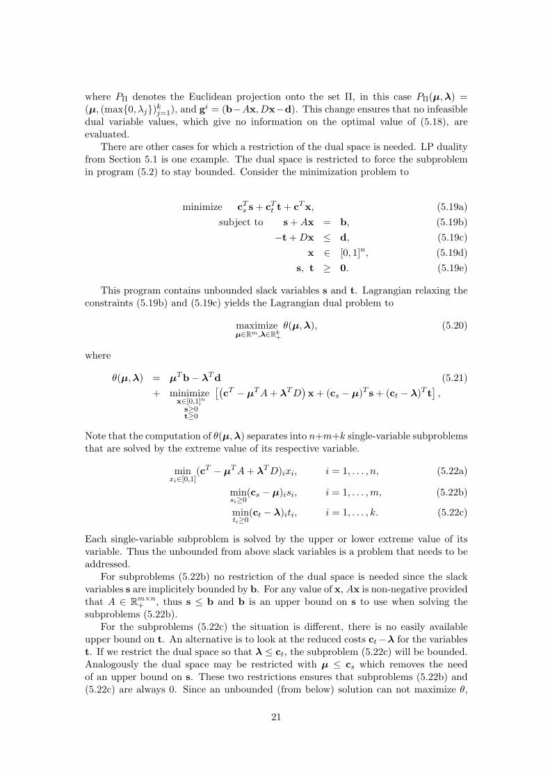
There are other cases for which a restriction of the dual space is needed. LP dualityfrom Section 5.1 is one example. The dual space is restricted to force the subproblemin program (5.2) to stay bounded. Consider the minimization problem to

minimize cTs s + cT

t t + cTx, (5.19a)

subject to s + Ax = b, (5.19b)

−t + Dx ≤ d, (5.19c)

x ∈ [0, 1]n, (5.19d)

s, t ≥ 0. (5.19e)

This program contains unbounded slack variables s and t. Lagrangian relaxing theconstraints (5.19b) and (5.19c) yields the Lagrangian dual problem to

maximizeµ∈Rm,λ∈R

k+

θ(µ, λ), (5.20)

where

θ(µ, λ) = µTb − λTd (5.21)

+ minimizex∈[0,1]n

s≥0t≥0

[(

cT − µT A + λT D)

x + (cs − µ)T s + (ct − λ)T t]

,

Note that the computation of θ(µ, λ) separates into n+m+k single-variable subproblemsthat are solved by the extreme value of its respective variable.

minxi∈[0,1]

(cT − µT A + λT D)ixi, i = 1, . . . , n, (5.22a)

minsi≥0

(cs − µ)isi, i = 1, . . . , m, (5.22b)

minti≥0

(ct − λ)iti, i = 1, . . . , k. (5.22c)

Each single-variable subproblem is solved by the upper or lower extreme value of itsvariable. Thus the unbounded from above slack variables is a problem that needs to beaddressed.

For subproblems (5.22b) no restriction of the dual space is needed since the slackvariables s are implicitely bounded by b. For any value of x, Ax is non-negative providedthat A ∈ R

m×n+ , thus s ≤ b and b is an upper bound on s to use when solving the

subproblems (5.22b).For the subproblems (5.22c) the situation is different, there is no easily available

upper bound on t. An alternative is to look at the reduced costs ct−λ for the variablest. If we restrict the dual space so that λ ≤ ct, the subproblem (5.22c) will be bounded.Analogously the dual space may be restricted with µ ≤ cs which removes the needof an upper bound on s. These two restrictions ensures that subproblems (5.22b) and(5.22c) are always 0. Since an unbounded (from below) solution can not maximize θ,

21

this restriction of the dual space yields an optimization problem that is equivalent to(5.20), which can then be stated as to

maximize θ(µ, λ),

such that µ ≤ cs,

0 ≤ λ ≤ ct,

where

θ(µ, λ) = bT µ − dT λ +

n∑

j=1

minxj∈[0,1]

(cT − µT A + λT D)jxj .

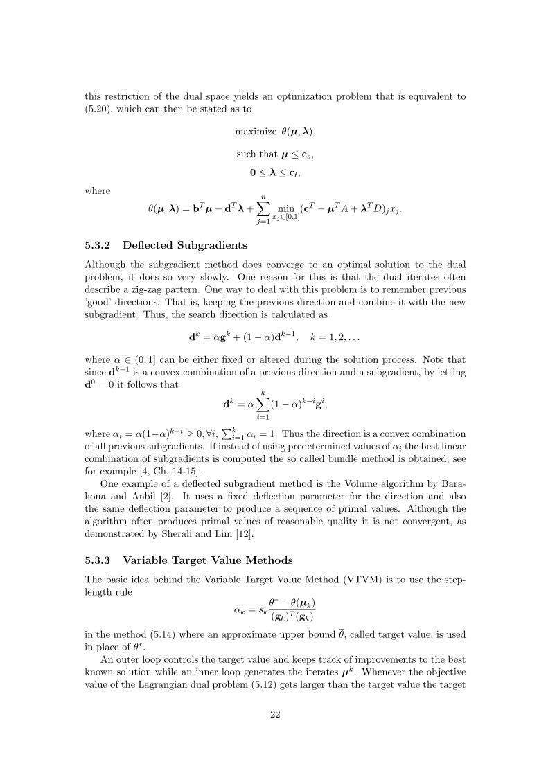
5.3.2 Deflected Subgradients

Although the subgradient method does converge to an optimal solution to the dualproblem, it does so very slowly. One reason for this is that the dual iterates oftendescribe a zig-zag pattern. One way to deal with this problem is to remember previous’good’ directions. That is, keeping the previous direction and combine it with the newsubgradient. Thus, the search direction is calculated as

dk = αgk + (1 − α)dk−1, k = 1, 2, . . .

where α ∈ (0, 1] can be either fixed or altered during the solution process. Note thatsince dk−1 is a convex combination of a previous direction and a subgradient, by lettingd0 = 0 it follows that

dk = αk

∑

i=1

(1 − α)k−igi,

where αi = α(1−α)k−i ≥ 0,∀i,∑k

i=1 αi = 1. Thus the direction is a convex combinationof all previous subgradients. If instead of using predetermined values of αi the best linearcombination of subgradients is computed the so called bundle method is obtained; seefor example [4, Ch. 14-15].

One example of a deflected subgradient method is the Volume algorithm by Bara-hona and Anbil [2]. It uses a fixed deflection parameter for the direction and alsothe same deflection parameter to produce a sequence of primal values. Although thealgorithm often produces primal values of reasonable quality it is not convergent, asdemonstrated by Sherali and Lim [12].

5.3.3 Variable Target Value Methods

The basic idea behind the Variable Target Value Method (VTVM) is to use the step-length rule

αk = sk

θ∗ − θ(µk)

(gk)T (gk)

in the method (5.14) where an approximate upper bound θ, called target value, is usedin place of θ∗.

An outer loop controls the target value and keeps track of improvements to the bestknown solution while an inner loop generates the iterates µk. Whenever the objectivevalue of the Lagrangian dual problem (5.12) gets larger than the target value the target

22

value is increased. If the inner loop has not managed to generate any good iterates thetarget value is decreased. This ensures that the target value is neither too high nor toolow, following the reasoning of step lengths from the beginning of this section. As longas the target value stays below θ∗ when it is increased the method will tend to a bettervalue. If the target value is increased above θ∗ it might be necessary to decrease it tosee an improvement in convergence. See Section (6.1) for a step by step description ofthe algorithm.

VTVM is a general convergent algorithm for nondifferential convex optimizationand can be used in combination with many different step direction strategies. See [11]for VTVM and [12] for VTVM in combination with the volume algorithm for linearprograms.

23

Chapter 6

Computational Tests and Results

This chapter contains computational results from using the VTVM on linear programsfrom crew rostering problems. Tests are done on stand alone problems comparingsolution quality and speed with that of XPress as well as solving the RMP during fullcolumn generation runs. The next section gives a detailed explanation of the algorithmVTVM. Section 6.2 describes the different test cases used. The following two sectionscompares the algorithm with XPress’s simplex and barrier algorithms.

6.1 The Algorithm

The idea behind the Variable Target Value Method (VTVM) is described in the previouschapter. In this section the actual algorithm will be stated, including the parametervalues used in the test-runs.

For a dual vector µi we denote the objective value to the Lagrangian subproblemθi = θ(µi). For this iteration xi ∈ arg minx∈X L(µi,x) solves the subproblem andgi = b − Axi is a subgradient to θ at µi. The algorithm is then as follows [12]:

(0) Initialize the parameters ǫ0 ≥ 0, ǫ > 0, kmax, β ∈ (0, 1], σ ∈ (0, 1/3], r ∈ (0, 1),r = r + 1, and τ , γ, η ∈ (0, 1]. In this implementation we use ǫ0 = 10−6, ǫ =0.1, kmax = 3000, β = 0.8, σ = 0.15, r = 0.1, τ = 75, γ = 20 and η = 0.75. Choosean initial solution µ1 (possibly from a warm start) and determine θi and gi. Setµ = µ1 and g = g1 and the best objective value known z1 = θ1. If ||g1|| < ǫ0terminate. Initialize l = k = 1, τ = γ = δ = 0 and RESET = 1. Initialize thetarget value w1 = min{UB, θ1 + ||g1||2/2} where UB is a known upper bound toθ(µ), at worst UB= ∞. Set ǫ1 = σ(w1 − θ1).

(1) If RESET = 1 set the search direction dk = gk, else dk = αgk+(1−α)dk−1, whereβ ≤ α ≤ 1. If ||dk|| = 0 set dk = gk. Set the steplength s = β(wl − θk)/||d

k||2

and set µk+1 = PΠ(µk + sdk), where PΠ denotes Euclidean projection onto thedual space. Increment τ and k by 1, set RESET = 0, and compute θk and gk.

(2) If θk > zk−1, set δ = δ + (θk − zk−1), zk = θk, µ = µk, g = gk, and γ = 0, and goto step 3. Otherwise set zk = zk−1, increment γ by 1, and go to step 4.

(3) If k > kmax or ||gk|| < ǫ0, terminate. If zk ≥ wl − ǫl, go to step 5, if τ ≥ τ go tostep 6, otherwise return to step 1.

24

(4) If k > kmax terminate. If γ ≥ γ or τ ≥ τ go to step 6. Else, return to step 1.

(5) Compute wl+1 = zk + max{ǫl + ηδ, r|zk|}. If r|zk| > ǫl + ηδ set r = r/r. Letǫl+1 = max{(wl+1 − zk)σ, ǫ}, put τ = δ = 0, and increment l by 1. Return to step1.

(6) Compute wl+1 = (zk + ǫl + wl)/2 and ǫl+1 = max{(wl+1 − zk)σ, ǫ}. If γ ≥ γ, thenset γ = max{γ + 10, 50}. If (wl −wl+1) ≤ 0.1, then set β = max{β/2, 10−6}. Putγ = τ = δ = 0 and increment l by 1. Reset µk = µ, θk = zk,g

k = g and putRESET = 1. Return to step 1.

Various strategies can be used for the deflection parameter α. Here we use α = 1for most cases. This basically turns the algorithm into a pure subgradient algorithmwith an elaborate scheme for calculating the steplength. Of course, the parameters may(and should) be tuned for the problem type solved.

In practice, the following termination criterion is added to the implementation: Ifan improvement occurs, but the improvement is smaller than some tolerance, the dualvariable is assumed to be close to an optimal point and the algorithm is terminated.

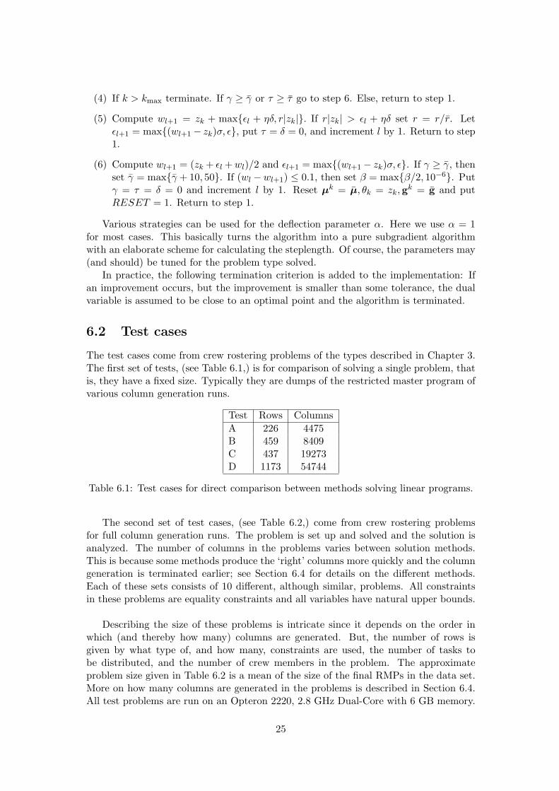
6.2 Test cases

The test cases come from crew rostering problems of the types described in Chapter 3.The first set of tests, (see Table 6.1,) is for comparison of solving a single problem, thatis, they have a fixed size. Typically they are dumps of the restricted master program ofvarious column generation runs.

Test Rows Columns

A 226 4475B 459 8409C 437 19273D 1173 54744

Table 6.1: Test cases for direct comparison between methods solving linear programs.

The second set of test cases, (see Table 6.2,) come from crew rostering problemsfor full column generation runs. The problem is set up and solved and the solution isanalyzed. The number of columns in the problems varies between solution methods.This is because some methods produce the ‘right’ columns more quickly and the columngeneration is terminated earlier; see Section 6.4 for details on the different methods.Each of these sets consists of 10 different, although similar, problems. All constraintsin these problems are equality constraints and all variables have natural upper bounds.

Describing the size of these problems is intricate since it depends on the order inwhich (and thereby how many) columns are generated. But, the number of rows isgiven by what type of, and how many, constraints are used, the number of tasks tobe distributed, and the number of crew members in the problem. The approximateproblem size given in Table 6.2 is a mean of the size of the final RMPs in the data set.More on how many columns are generated in the problems is described in Section 6.4.All test problems are run on an Opteron 2220, 2.8 GHz Dual-Core with 6 GB memory.

25

Test set Description Approximate sizerows, columns

bos 25 Boston, 25 crew 220, 4400atl 95 Atlanta, 95 crew 460, 8600bos 50 Boston, 50 crew 440, 19000atl 254 Atlanta, 254 crew 1170, 50000

Table 6.2: Test sets for column generation with ten test cases in each set. Solving aproblem determines monthly rosters for all crew in the problem.

6.3 Comparison with XPress

The behavior of the LP solver determines the success of a column generator. A fast LPsolver that produces dual variable values which in turn generate bad columns may beworse than a slow LP solver that generates good columns. In order to analyze how theVTVM performs within column generation it is necessary to know how it performs onsingle problems.

Table 6.3 shows runtimes for solving the four linear programs given in Table 6.1,solved by both the primal simplex method and the VTVM.

Test Runtime(s) Errorproblem The simplex method VTVM

A 1.0 1.19 8.0%B 3.12 1.22 1.7%C 23.15 3.19 9.5%D 193.31 10.82 8.2%

Table 6.3: Test results for single problems comparing the simplex method and VTVM.Error given by (θ∗−θk)/θ∗ where θ∗ is the optimal objective value and θk is the objectivevalue obtained at termination of the VTVM.

As seen in the table the VTVM becomes increasingly faster than the primal sim-plex method when the problem sizes increase. This is to be expected, since the simplexmethod solves several systems of linear equations while the most time consuming opera-tion in VTVM is matrix-vector multiplication.1 Additionally, VTVM in this implemen-tation terminates after a maximum of 3000 iterations, the simplex method may needmore iterations, i.e. more linear equations to solve, when the problem size increases.

The solution produced by VTVM is almost always sub-optimal, that is, has lowerobjective value compared to the optimal objective value. Further tuning of the param-eters given in Section 6.1 results in solutions with objective values closer to optimum atthe cost of longer runtimes. However, in the column generation scheme the improvedLP solution quality is not worth the increased runtime. Although the solution is sub-optimal the VTVM always produces a feasible dual solution and can be used to generatecolumns.

1Solving a system of linear equations with a sparse matrix (n columns) uses O(n2) basic, i.e. multi-plication and addition, operations. Sparse matrix-vector multiplication only uses O(n) basic operations.

26

6.4 Results within column generation

As seen in the previous section the speed of the VTVM LP solver is significantly fastercompared to the XPress simplex solver. The difference within column generation isnot quite as large since the warm-start for the simplex method is very effective2. Thebig gain comes from producing better dual solutions, thereby generating the correctcolumns earlier. This results in smaller RMPs to solve during column generation, earliertermination of the column generation algorithm, and a smaller integer program to solvewhen fixing is performed.

One problem with the subgradient method is that it does not produce primal variablevalues to be used for fixing variable values. Another is that while the subgradientmethod quickly generates good columns it performs poorly at the end of the columngeneration process. In the Jeppesen column generator several columns are generated ineach iteration. When the column generation process (where the RMP is solved by thesubgradient method) terminates, in many cases it does so after quite many iterations inwhich only a few columns have been generated. That is, it terminates after quite manyiterations without much improvement. To address these issues the LP solver switchesto the simplex method (using XPress) when the column generation scheme does notimprove much.

Figure 6.1 shows the total runtime of solving the LP relaxation using column gener-ation together with the primal and dual simplex methods (XPress), the barrier method(XPress) and the variable target value method. The barrier method and the VTVMproduce only dual values3. As evident in the figure the subgradient method does notalways perform better than the simplex method. The barrier method seems to be abetter choice over-all.

Although in some cases the only output required is a lower bound to the problem,for which a dual solution is sufficient, what is ultimately required is an integer solution.For this (continous) primal variable values constitute a good start to be used in variousfixing procedures. As mentioned above the VTVM is replaced by the simplex methodat the end of the column generation process to terminate the process earlier. Anotherresult of this is that primal values are also produced. For comparison reasons, thebarrier method runs a cross-over, also at the end of the column generation process, togenerate an optimal solution including both primal and dual variable values. Figure 6.2shows the result of this. With this change the VTVM is faster in all problem instances,even the smaller ones in the top figure. For the largest problems the column generationwith the VTVM is 40%-60% faster but even the smaller problems show significantimprovement. For even larger problems the difference between barrier and VTVM maybe larger since the barrier method includes more complex operations than VTVM, suchas linear equation solving.

The convergence of the column generation process is shown in Figures 6.3 and 6.4

2If this was not the case the difference in time between using the simplex method and the subgradientmethod in the column generation algorithm would be far greater. Consider that the subgradient methodis about 20 times faster than the simplex method on the largest stand alone problem of the previoussection, a problem of corresponding final size is solved about twice as fast with VTVM compared to thesimplex method during the column generation run. See Figure 6.2.

3The barrier method is a primal-dual method and produces both primal and dual values. However,since it is an approximate method the objective value given by the dual variable values is lower thanthe value of any feasible primal solution. Thus there are no primal values corresponding to the lowerbound and the dual values.

27

for two instances in the data sets. Using the subgradient method the column generationprocess is near convergence before the duals produced by the simplex method producecolumns that result in improvement. The spikes in the figures are due to the subgradientmethod being an approximate method so it may terminate suboptimally. That thesubgradient method on rare occations terminates very suboptimal during the columngeneration process is not a problem. At worst a few unnecessary columns are addedand in the next iteration the subgradient method will most probably not terminatetoo early on the modified RMP. These figures show the strength of the VTVM in thiscontext. Duals produced generating the correct columns early as seen by the figure withobjective value versus iteration

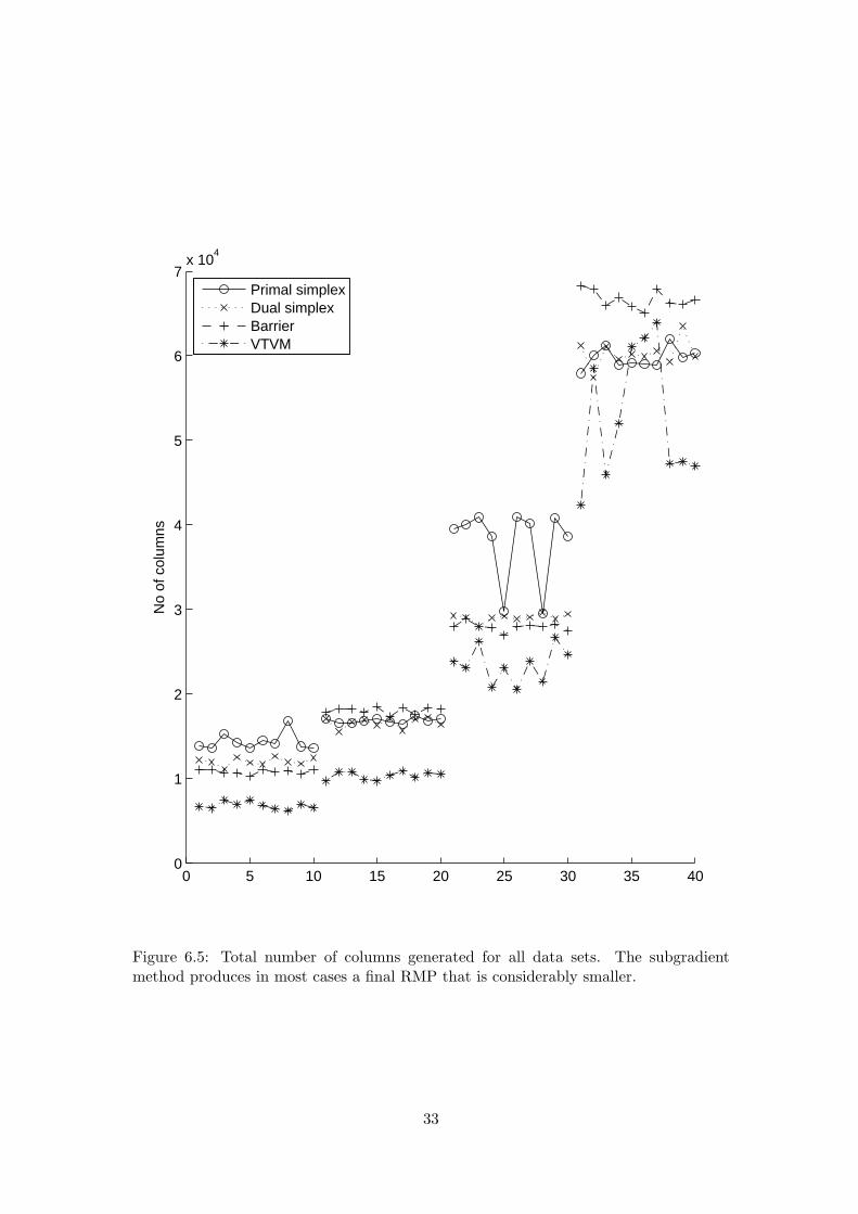
The number of columns generated in each instance is shown in Figure 6.5. The totalnumber of columns affect the speed of the RMP solver as well as the fixing procedureafter the LP relaxation has been solved. How many columns the final RMP consistsof is dependant on the number of column generation iterations, but also how many ofthose iterations generate ’many’ columns.

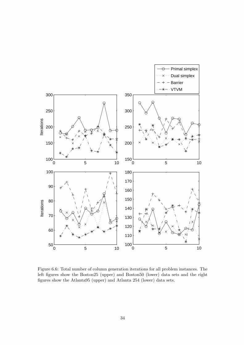
Figure 6.6 shows the number of column generation iterations for each problem in-stance. As seen in the figure the VTVM uses in most cases fewer iterations. This ofcourse affects the total runtime. However, all problems in the data sets have fairly easyrules and fast pricing problems (generating columns). Thus, a problem with a moredifficult pricing problem should be solved relatively even faster using the VTVM tosolve the restricted master problem.

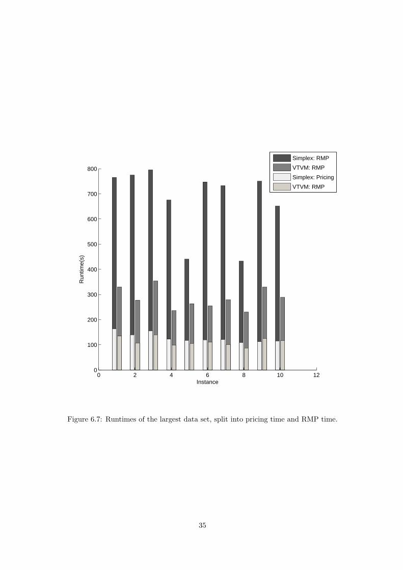
Finally, Figure 6.7 shows the runtime for the largest data set (Atlanta 254) splitinto the time for pricing and for RMP. As seen in Figure 6.6, for this data set thenumber of column generation iterations is about the same for both simplex and VTVM.As expected the time spent in the pricer is about the same for these methods as well.Using VTVM to solve the RMP the time spent solving the RMP improves greatly.Using the Simplex method, up to 85% of the runtime is spent solving the RMP. For theVTVM, around 60% of the total runtime is spent solving the RMP. Add to this thatthe VTVM has the potential to use fewer column generation iterations, thus the totalruntime can be much improved.

28

0 5 1040

60

80

100

120

140

Tot

al r

untim

e (s

)

0 5 1040

60

80

100

120

140

0 5 10200

300

400

500

600

700

800

900

1000

Tot

al r

untim

e (s

)

0 5 10500

1000

1500

2000

2500

Primal simplex

Dual simplex

Barrier

VTVM

Figure 6.1: Runtimes for the four methods for solving the LP relaxation. The barriermethod and VTVM produce only dual variable values. The figures to the left showruntimes for Boston25 (upper) and Boston50 (lower) test sets. The figures to the rightshow runtimes for Atlanta95 (upper) and Atlanta254 (lower) test sets.

29

0 5 1020

40

60

80

100

120

140

Tot

al r

untim

e (s

)

0 5 1040

60

80

100

120

0 5 10200

400

600

800

1000

Tot

al r

untim

e (s

)

0 5 10500

1000

1500

2000

2500

Primal simplex

Dual simplex

Barrier

VTVM

Figure 6.2: Runtimes for the four methods solving the LP relaxation. These are thesame test cases as in Figure 6.2. The only difference is that instead of VTVM and thebarrier method, the column generation scheme always uses the simplex method at theend when not much improvement is made. This yields primal values at termination aswell as faster convergence for VTVM.

30

0 20 40 60 80 100 120 140 160−2

−1.8

−1.6

−1.4

−1.2x 10

5

Iteration

Obj

ectiv

e

Primal simplexDual simplexBarrierVTVM

0 500 1000 1500 2000−2

−1.8

−1.6

−1.4

−1.2x 10

5

Total runtime (s)

Obj

ectiv

e

Primal simplexDual simplexBarrierVTVM

Figure 6.3: Convergence in column generation for one instance of the Atlanta254 dataset. The subgradient method generates the correct columns earlier and is almost con-verged when the dual from the simplex method starts producing the correct columns.The upper figure displays objective value versus iteration number and the lower figuredisplays objective value versus total runtime.

31

0 50 100 150 200 250 300−3.5

−3

−2.5

−2

−1.5

−1x 10

4

Iteration

Obj

ectiv

e

0 100 200 300 400 500 600 700 800 900−3.5

−3

−2.5

−2

−1.5

−1x 10

4

Total runtime (s)

Obj

ectiv

e

Primal simplexDual simplexBarrierVTVM

Primal simplexDual simplexBarrierVTVM

Figure 6.4: Convergence in column generation for one instance of the Boston50 dataset.

32

0 5 10 15 20 25 30 35 400

1

2

3

4

5

6

7x 10

4

No

of c

olum

ns

Primal simplexDual simplexBarrierVTVM

Figure 6.5: Total number of columns generated for all data sets. The subgradientmethod produces in most cases a final RMP that is considerably smaller.

33

0 5 10100

150

200

250

300

Itera

tions

0 5 10150

200

250

300

350

0 5 1050

60

70

80

90

100

Itera

tions

0 5 10100

110

120

130

140

150

160

170

180

Primal simplex

Dual simplex

Barrier

VTVM

Figure 6.6: Total number of column generation iterations for all problem instances. Theleft figures show the Boston25 (upper) and Boston50 (lower) data sets and the rightfigures show the Atlanta95 (upper) and Atlanta 254 (lower) data sets.

34

0 2 4 6 8 10 120

100

200

300

400

500

600

700

800

Instance

Run

time(

s)

Simplex: RMP

VTVM: RMP

Simplex: Pricing

VTVM: RMP

Figure 6.7: Runtimes of the largest data set, split into pricing time and RMP time.

35

Chapter 7

Conclusions

A variable target value method has been implemented and tested in a column generationsetting for crew rostering problems. For solving stand alone problems the method inthis implementation performs many times faster than the simplex method. However,this is at the cost of the solution not being optimal and without generating any primalsolutions. This suggests that the VTVM is effective for quickly producing a roughlower bound for linear programs. However, the lack of primal values and suboptimaltermination make the VTVM a poor choice for solving linear programs.

On the other hand, when used in a column generation setting the method performsvery well, resulting in earlier convergence of the column generation and in smaller prob-lems to solve in fixing procedures. Combining the VTVM with the simplex methodterminates the column generation process faster as well as producing primal valuesto use for fixing. The method is faster with respect to both runtime and number ofiterations, which is promising for its use in solving more difficult pricing problems.

Comparing the subgradient method to the barrier method, the subgradient methodrequires less memory and results in totally fewer columns generated. Thus the memoryrequirements in total is much smaller when using the subgradient method.

In conclusion the VTVM performs very well within a column generation context,with regard to both computational speed and memory requirements. When combinedwith the simplex method a nearly seamless change of LP optimizer may be made, thatis, the solution quality is equivalent and primal solutions are generated. Runtimes havebeen cut in half for full column generation runs, where most of the time earned comesfrom solving the RMP more efficiently. However, only a few less iterations of the columngeneration scheme — which often happens when using the VTVM — may result in adrastic reduction of total runtime due to the size of the final RMP.

Further development may include a development of the algorithm to produce near-feasible primal solutions analogously with the volume method. These primal solutionscould then be used in a fixing procedure to obtain a near-optimal integer solution.

36

Bibliography

[1] N. Andreasson, A. Evgrafov, and M. Patriksson. An Introduction to ContinuousOptimization. Studentlitteratur, Lund, 2005.

[2] F. Barahona and R. Anbil. The volume algorithm: Producing primal solutionswith a subgradient method. Mathematical Programming, 87(3):385–399, 2000.

[3] G. Desaulniers, J. Desrosiers, and M. Solomon. Column Generation. Springer, NewYork, 2005.

[4] J.-B. Hiriart-Urruty and C. Lemarechal. Convex Analysis and Minimization Algo-rithms II. Springer-Verlag, Berlin, 1993.

[5] N. Kohl and S. E. Karisch. Airline crew rostering: Problem types, modeling andoptimization. Annals of Operations Research, 127:223–257, 2004.

[6] L. S. Lasdon. Optimization theory for large systems. MacMillan, New York, 1970.

[7] C. Lim and H. D. Sherali. Convergence and computational analyses for some vari-able target value and subgradient deflection methods. Computational Optimizationand Applications, 34(3):409–428, 2006.

[8] M. E. Lubbecke and J. Desrosiers. Selected topics in column generation. OperationsResearch, 53(6):1007–1023, 2005.

[9] K. G. Murty. Linear Programming. John Wiley & Sons, New York, 1983.

[10] B. T. Polyak. Minimization of unsmooth functionals. USSR Computational Math-ematics and Mathematical Physics, 9:14–29, 1969.

[11] H. D. Sherali, G. Choi, and C. H. Tuncbilek. A variable target value method fornondifferentiable optimization. Operations Research Letters, 26:1–8, 2000.

[12] H. D. Sherali and C. Lim. On embeding the volume algorithm in a variable targetvalue method. Operations Research Letters, 32:455–462, 2004.

[13] L. A. Wolsey. Integer Programming. John Wiley & Sons, New York, 1998.

37