Essentialformulaes3-euw1-ap-pe-ws4-cws-documents.ri-prod.s3.amazonaws.com/... · Essentialformulae...

Essential formulae

Number and algebra

Laws of indices:

am × an = am+n am

an= am−n (am)n = amn

amn = n

√am a−n = 1

ana0 = 1

Quadratic formula:

If ax2 + bx + c = 0 then x = −b ± √b2 − 4ac

2a

Factor theorem:

If x =a is a root of the equation f (x)=0, then (x −a)is a factor of f (x).

Remainder theorem:If (ax2 +bx +c) is divided by (x − p), theremainder will be: ap2 +bp +c

or if (ax3 +bx2 +cx +d) is divided by (x − p), theremainder will be: ap3 +bp2 +cp +d

Partial fractions:

Provided that the numerator f (x) is of less degree thanthe relevant denominator, the following identities aretypical examples of the form of partial fractions used:

f (x)

(x + a)(x + b)(x + c)

≡ A

(x + a)+ B

(x + b)+ C

(x + c)

f (x)

(x + a)3(x + b)

≡ A

(x + a)+ B

(x + a)2+ C

(x + a)3+ D

(x + b)

f (x)

(ax2 + bx + c)(x + d)

≡ Ax + B

(ax2 + bx + c)+ C

(x + d)

Definition of a logarithm:

If y =ax then x = loga y

Laws of logarithms:

log(A × B)= log A + log B

log

(A

B

)

= log A − log B

log An = n × log A

Exponential series:

ex = 1 + x + x2

2!+ x3

3!+ ·· ·

(valid for all values of x)

Hyperbolic functions:

sinh x = ex − e−x

2cosech x = 1

sinh x= 2

ex − e−x

cosh x = ex + e−x

2sech x = 1

cosh x= 2

ex + e−x

tanh x = ex − e−x

ex + e−xcoth x = 1

tanh x= ex + e−x

ex − e−x

cosh2 x − sinh2 =1 1 − tanh2 x = sech2 x

coth2 x − 1 = cosech2 x

Higher Engineering Mathematics. 978-0-415-66282-6, © 2014 John Bird. Published by Taylor & Francis. All rights reserved.

Essential formulae 815

Arithmetic progression:

If a =first term and d =common difference, then thearithmetic progression is: a, a +d , a +2d , . . .

The nth term is: a +(n −1)d

Sum of n terms, Sn = n

2[2a +(n −1)d]

Geometric progression:

If a =first term and r =common ratio, then the geomet-ric progression is: a, ar , ar2, . . .

The nth term is: arn−1

Sum of n terms, Sn = a(1−rn)

(1−r)or

a(rn −1)

(r −1)

If −1<r<1, S∞ = a

(1−r)

Binomial series:

(a + b)n = an + nan−1b + n(n − 1)

2!an−2b2

+ n(n − 1)(n − 2)

3!an−3b3 + ·· ·

(1 + x)n = 1 + nx + n(n − 1)

2!x2

+ n(n − 1)(n − 2)

3!x3 + ·· ·

Maclaurin’s series:

f (x)= f (0)+ x f ′(0)+ x2

2!f ′′(0)

+ x3

3!f ′′′(0)+ ·· ·

Newton–Raphson iterative method:

If r1 is the approximate value for a real root of the equa-tion f (x)=0, then a closer approximation to the root,r2, is given by:

r2 = r1 − f (r1)

f ′(r1)

Boolean algebra:

Laws and rules of Boolean algebra

Commutative laws: A+ B = B + A

A · B = B · A

Associative laws: A+ B +C = (A+ B)+C

A · B ·C = (A · B) ·CDistributive laws: A · (B +C)= A · B + A ·C

A+(B ·C)= (A+ B) ·(A+C)

Sum rules: A+ A =1

A+1=1

A+0= A

A+ A = A

Product rules: A · A =0

A ·0=0

A ·1= A

A · A = A

Absorption rules: A+ A · B = A

A ·(A+ B)= A

A+ A · B = A+ B

De Morgan’s laws: A+ B = A · B

A · B = A+ B

Geometry and trigonometry

Theorem of Pythagoras:

b2 = a2 + c2

A

B C

cb

a

Figure FA1

Identities:

secθ = 1

cosθcosec θ= 1

sinθ

cotθ = 1

tanθtanθ = sin θ

cosθ

cos2 θ + sin2 θ = 1 1 + tan2 θ = sec2 θ

cot2 θ + 1 = cosec2 θ

816 Higher Engineering Mathematics

Triangle formulae:

With reference to Fig. FA2:

Sine rulea

sin A= b

sin B= c

sin C

Cosine rule a2 =b2 + c2 − 2bc cos A

A

B C

c

a

b

Figure FA2

Area of any triangle

(i) 12 × base × perpendicular height

(ii) 12 ab sinC or 1

2 ac sin B or 12 bc sin A

(iii)√

[s(s −a)(s −b)(s −c)] where s = a +b+c

2

Compound angle formulae:

sin(A ± B)= sin A cos B ± cos A sin B

cos(A ± B)= cos A cos B ∓ sin A sin B

tan(A ± B)= tan A ± tan B

1 ∓ tan A tan B

If R sin (ωt+α)=a sin ωt+b cos ωt,

then a = R cosα, b = R sinα,

R =√(a2 + b2) and α = tan−1 b

a

Double angles:

sin 2A = 2 sin A cos A

cos2A = cos2 A − sin2 A = 2 cos2 A − 1

= 1 − 2 sin2 A

tan 2A = 2 tan A

1 − tan2 A

Products of sines and cosines into sums ordifferences:

sin A cos B = 12 [sin(A + B)+ sin(A − B)]

cos A sin B = 12 [sin(A + B)− sin(A − B)]

cos A cos B = 12 [cos(A + B)+ cos(A − B)]

sin A sin B = − 12 [cos(A + B)−cos(A − B)]

Sums or differences of sines and cosinesinto products:

sin x + sin y = 2 sin

(x + y

2

)

cos

(x − y

2

)

sin x − sin y = 2 cos

(x + y

2

)

sin

(x − y

2

)

cos x + cos y = 2 cos

(x + y

2

)

cos

(x − y

2

)

cos x − cos y = −2 sin

(x + y

2

)

sin

(x − y

2

)

For a general sinusoidal functiony=Asin(ωt±α), then:

A = amplitude

ω = angular velocity = 2π f rad/s

2π

ω= periodic time T seconds

ω

2π= frequency, f hertz

α = angle of lead or lag (compared withy = A sinωt)

Cartesian and polar co-ordinates:

If co-ordinate (x, y)=(r,θ) then r =√

x2 + y2 and

θ= tan−1 y

xIf co-ordinate (r,θ)= (x, y) then x =r cosθ andy =r sinθ


The circle:

With reference to Fig. FA3.

Area = πr2 Circumference = 2πr

π radians = 180◦

sr

r

�

Figure FA3

For sector of circle:

s = rθ (θ in rad)

shaded area= 12r2θ (θ in rad)

Equation of a circle, centre at (a, b), radius r :

(x − a)2 + (y − b)2 = r2

Linear and angular velocity:

If v= linear velocity (m/s), s =displacement (m),t = time (s), n =speed of revolution (rev/s),θ=angle (rad), ω=angular velocity (rad/s),r = radius of circle (m) then:

v = s

tω = θ

t= 2πn v = ωr

centripetal force = mv2

r

where m =mass of rotating object.

Graphs

Equations of functions:

Equation of a straight line: y =mx +c

Equation of a parabola: y =ax2 +bx +c

Circle, centre (a, b), radius r:

(x −a)2 +(y −b)2 =r2

Equation of an ellipse, centre at origin, semi-axes a

and b:x2

a2 + y2

b2 =1

Equation of a hyperbola:x2

a2 − y2

b2 =1

Equation of a rectangular hyperbola: xy =c2

Irregular areas:

Trapezoidal rule

Area ≈(

width ofinterval

)[1

2

(first + lastordinates

)

+(

sum of remainingordinates

)]

Mid-ordinate rule

Area ≈(

width ofinterval

)(sum of

mid-ordinates

)

Simpson’s rule

Area ≈ 1

3

(width ofinterval

)[(first + lastordinate

)

+4

(sum of even

ordinates

)

+2

(sum of remaining

odd ordinates

)]

Vector geometry

If a=a1i+a2 j+a3 k and b=b1 i+b2 j+b3 k

a · b = a1b1 + a2b2 + a3b3

|a | =√

a21 + a2

2 + a23 cosθ = a · b

|a| |b|

a × b =∣∣∣∣∣∣

i j ka1 a2 a3b1 b2 b3

∣∣∣∣∣∣

|a × b | =√

[(a · a)(b · b)− (a · b)2]


Complex numbers

z =a + jb=r(cosθ+ j sinθ)=r∠θ=re jθ wherej2 =−1

Modulus r =|z|=√(a2 +b2)

Argument θ=arg z = tan−1 b

a

Addition: (a + jb)+(c+ jd)=(a +c)+ j (b+d)

Subtraction: (a + jb)−(c + jd)=(a −c)+ j (b −d)

Complex equations: If m + jn = p + jq then m = pand n =q

Multiplication: z1 z2 =r1 r2∠(θ1 +θ2)

Division:z1

z2= r1

r2∠(θ1 −θ2)

De Moivre’s theorem:

[r∠θ ]n =rn∠nθ=rn(cosnθ+ j sin nθ)=re jθ

Matrices and determinants

Matrices:

If A =(

a bc d

)

and B =(

e fg h

)

then

A + B =(

a + e b + f

c + g d + h

)

A − B =(

a − e b − f

c − g d − h

)

A × B =(

ae + bg a f + bh

ce + dg cf + dh

)

A−1 = 1

ad − bc

(d −b

−c a

)

If A=

⎛

⎜⎝

a1 b1 c1

a2 b2 c2

a3 b3 c3

⎞

⎟⎠ then A−1 = BT

|A| where

BT = transpose of cofactors of matrix A

Determinants:∣∣∣∣a bc d

∣∣∣∣= ad − bc

∣∣∣∣∣∣

a1 b1 c1a2 b2 c2a3 b3 c3

∣∣∣∣∣∣= a1

∣∣∣∣b2 c2b3 c3

∣∣∣∣− b1

∣∣∣∣a2 c2a3 c3

∣∣∣∣

+ c1

∣∣∣∣a2 b2a3 b3

∣∣∣∣

Differential calculus

Standard derivatives:

y or f (x)dy

dxor f ′(x)

axn anxn−1

sin ax a cosax

cosax −a sin ax

tan ax a sec2 ax

secax a secax tan ax

cosecax −a cosecax cot ax

cot ax −a cosec 2 ax

eax aeax

ln ax1

x

sinh ax a coshax

cosh ax a sinhax

tanhax a sech 2 ax

sech ax −a sech ax tanh ax

cosechax −a cosechax cothax

cothax −a cosech 2ax

sin−1 x

a

1√a2 − x2

sin−1 f (x)f ′(x)

√1 − [ f (x)]2

cos−1 x

a

−1√a2 − x2


y or f (x)dy

dxor f ′(x)

cos−1 f (x)− f ′(x)

√1 − [ f (x)]2

tan−1 x

a

a

a2 + x2

tan−1 f (x)f ′(x)

1 + [ f (x)]2

sec−1 x

a

a

x√

x2 − a2

sec−1 f (x)f ′(x)

f (x)√

[ f (x)]2 − 1

cosec−1 x

a

−a

x√

x2 − a2

cosec−1 f (x)− f ′(x)

f (x)√

[ f (x)]2 − 1

cot−1 x

a

−a

a2 + x2

cot−1 f (x)− f ′(x)

1 + [ f (x)]2

sinh−1 x

a

1√x2 + a2

sinh−1 f (x)f ′(x)

√[ f (x)]2 + 1

cosh−1 x

a

1√x2 − a2

cosh−1 f (x)f ′(x)

√[ f (x)]2 − 1

tanh−1 x

a

a

a2 − x2

tanh−1 f (x)f ′(x)

1 − [ f (x)]2

sech−1 x

a

−a

x√

a2 − x2

sech−1 f (x)− f ′(x)

f (x)√

1 − [ f (x)]2

y or f (x)dy

dxor f ′(x)

cosech−1 x

a

−a

x√

x2 + a2

cosech−1 f (x)− f ′(x)

f (x)√

[ f (x)]2 + 1

coth−1 x

a

a

a2 − x2

coth−1 f (x)f ′(x)

1 − [ f (x)]2

Product rule:

When y =uv and u and v are functions of x then:

dydx

=udv

dx+v

dudx

Quotient rule:

When y = u

vand u and v are functions of x then:

dydx

=v

dudx

−udv

dxv2

Function of a function:

If u is a function of x then:

dydx

= dydu

× dudx

Parametric differentiation:

If x and y are both functions of θ , then:

dydx

=dydθdxdθ

andd2ydx2 =

ddθ

(dydx

)

dxdθ

Implicit function:

ddx

[ f (y)]= ddy

[ f (y)]× dydx


Maximum and minimum values:

If y = f (x) thendydx

=0 for stationary points.

Let a solution ofdy

dx=0 be x =a; if the value of

d2 y

dx2 when x =a is: positive, the point is a minimum,

negative, the point is a maximum.

Velocity and acceleration:

If distance x = f (t), then

velocity v= f ′(t) ordx

dtand

acceleration a = f ′′(t) ord2x

dt2

Tangents and normals:

Equation of tangent to curve y = f (x) at the point(x1, y1) is:

y − y1 = m(x − x1)

where m =gradient of curve at (x1, y1).

Equation of normal to curve y = f (x) at the point(x1, y1) is:

y − y1 = − 1

m(x − x1)

Partial differentiation:

Total differentialIf z = f (u,v, . . .), then the total differential,

dz = ∂z

∂udu + ∂z

∂vdv + . . . .

Rate of change

If z = f (u,v, . . .) anddu

dt,

dv

dt, … denote the rate of

change of u, v, … respectively, then the rate of changeof z,

dz

dt= ∂z

∂u· du

dt+ ∂z

∂v· dv

dt+ . . .

Small changesIf z = f (u,v, . . .) and δx , δy, … denote small changesin x , y, … respectively, then the corresponding change,

δz ≈ ∂z

∂xδx + ∂z

∂yδy + . . . .

To determine maxima, minima and saddle points forfunctions of two variables: Given z = f (x, y),

(i) determine∂z

∂xand

∂z

∂y

(ii) for stationary points,∂z

∂x=0 and

∂z

∂y=0

(iii) solve the simultaneous equations∂z

∂x=0 and

∂z

∂y=0 for x and y, which gives the co-ordinates

of the stationary points

(iv) determine∂2z

∂x2 ,∂2z

∂y2 and∂2z

∂x∂y

(v) for each of the co-ordinates of the station-ary points, substitute values of x and y into

∂2z

∂x2 ,∂2z

∂y2 and∂2z

∂x∂yand evaluate each

(vi) evaluate

(∂2z

∂x∂y

)2

for each stationary point,

(vii) substitute the values of∂2z

∂x2 ,∂2z

∂y2 and∂2z

∂x∂yinto

the equation �=(∂2z

∂x∂y

)2

−(∂2z

∂x2

)(∂2z

∂y2

)

and evaluate

(viii) (a) if �>0 then the stationary point is a saddlepoint

(b) if �<0 and∂2z∂x2 <0, then the stationary

point is a maximum point, and

(c) if �<0 and∂2z∂x2 >0, then the stationary

point is a minimum point


Integral calculus

Standard integrals:

y∫

y dx

axn axn+1

n + 1+ c

(except where n = −1)

cosax1

asin ax + c

sin ax − 1

acosax + c

sec2 ax1

atan ax + c

cosec2 ax − 1

acot ax + c

cosecax cot ax − 1

acosec ax + c

secax tan ax1

asecax + c

eax 1

aeax + c

1

xln x + c

tan ax1

aln(secax)+ c

cos2 x1

2

(

x + sin 2x

2

)

+ c

sin2 x1

2

(

x − sin 2x

2

)

+ c

tan2 x tan x − x + c

cot2 x −cot x − x + c

1√(a2 − x2)

sin−1 x

a+ c

√(a2 − x2)

a2

2sin−1 x

a+ x

2

√(a2 − x2)+ c

y∫

y dx

1

(a2 + x2)

1

atan−1 x

a+ c

1√(x2 + a2)

sinh−1 x

a+ c or

ln

[x +√(x2 + a2)

a

]

+ c

√(x2 + a2)

a2

2sinh−1 x

a+ x

2

√(x2 + a2)+ c

1√(x2 − a2)

cosh−1 x

a+ c or

ln

[x +√(x2 − a2)

a

]

+ c

√(x2 − a2)

x

2

√(x2 − a2)− a2

1cosh−1 x

a+ c

t= tanθ

2substitution:

To determine∫ 1

a cosθ + b sinθ + cdθ let

sinθ = 2t

(1 + t2)cosθ = 1 − t2

1 + t2 and

dθ = 2 dt

(1 + t2)

Integration by parts:

If u and v are both functions of x then:∫

udv

dxdx=uv−

∫v

dudx

dx

Reduction formulae:∫

xnex dx = In = xnex − nIn−1

∫xn cos x dx = In = xn sin x + nxn−1 cos x

−n(n − 1)In−2


∫ π

0xn cos x dx = In = −nπn−1 − n(n − 1)In−2

∫xn sin x dx = In = −xn cos x + nxn−1 sin x

−n(n − 1)In−2

∫sinn x dx = In = − 1

nsinn−1 x cos x + n − 1

nIn−2

∫cosn x dx = In = 1

ncosn−1 sin x + n − 1

nIn−2

∫ π/2

0sinn x dx =

∫ π/2

0cosn x dx = In = n − 1

nIn−2

∫tann x dx = In = tann−1 x

n − 1− In−2

∫(ln x)n dx = In = x(ln x)n − nIn−1

With reference to Fig. FA4.

y

y 5 f(x)

x 5 a x 5 b x0

A

Figure FA4

Area under a curve:

area A =∫ b

ay dx

Mean value:

mean value = 1

b − a

∫ b

ay dx

Rms value:

rms value =√{

1

b − a

∫ b

ay2 dx

}

Volume of solid of revolution:

volume =∫ b

aπy2 dx about the x-axis

Centroids:

With reference to Fig. FA5:

x =

∫ b

axy dx

∫ b

ay dx

and y =12

∫ b

ay2 dx

∫ b

ay dx

y

C

Area A

xy

y 5 f(x)

x 5 a x 5 b x0

Figure FA5

Theorem of Pappus:

With reference to Fig. FA5, when the curve is rotated onerevolution about the x-axis between the limits x =a andx =b, the volume V generated is given by: V = 2πAy

Parallel axis theorem:

If C is the centroid of area A in Fig. FA6 then

Ak2B B = Ak2

GG + Ad2 or k2B B = k2

GG + d2

G B

G B

d

C

Area A

Figure FA6


Second moment of area and radius of gyration:

Shape Position of axis Second moment Radius ofof area, I gyration, k

Rectangle (1) Coinciding with bbl3

3

1√3length l

(2) Coinciding with llb3

3

b√3

breadth b

(3) Through centroid,bl3

12

1√12parallel to b

(4) Through centroid,lb3

12

b√12parallel to l

Triangle (1) Coinciding with bbh3

12

h√6Perpendicular

(2) Through centroid,bh3

36

h√18

height h

parallel to basebase b

(3) Through vertex,bh3

4

h√2parallel to base

Circle (1) Through centre,πr4

2

r√2radius r perpendicular to plane

(i.e. polar axis)

(2) Coinciding with diameterπr4

4

r

2

(3) About a tangent5πr4

4

√5

2r

Semicircle Coinciding withπr4

8

r

2radius r diameter

Perpendicular axis theorem:

If OX and OY lie in the plane of area A in Fig. FA7,

then Ak2O Z = Ak2

O X + Ak2OY or k2

O Z = k2O X + k2

OY

Z

O

Y

X

Area A

Figure FA7

Numerical integration:

Trapezoidal rule

∫ydx ≈

(width ofinterval

)[1

2

(first + last

ordinates

)

+(

sum of remaining

ordinates

)]

Mid-ordinate rule

∫ydx ≈

(width ofinterval

)(sum of

mid-ordinates

)


Simpson’s rule

∫ydx ≈ 1

3

(width ofinterval

)[(first + lastordinate

)

+ 4

(sum of even

ordinates

)

+2

(sum of remaining

odd ordinates

)]

Differential equations

First-order differential equations:

Separation of variables

Ifdy

dx= f (x) then y =

∫f (x)dx

Ifdy

dx= f (y) then

∫dx =

∫dy

f (y)

Ifdy

dx= f (x) · f (y) then

∫dy

f (y)=∫

f (x)dx

Homogeneous equations:

If Pdy

dx= Q, where P and Q are functions of both x and

y of the same degree throughout (i.e. a homogeneousfirst-order differential equation) then:

(i) rearrange Pdy

dx= Q into the form

dy

dx= Q

P

(ii) make the substitution y =vx (where v is a func-tion of x), from which, by the product rule,

dy

dx= v(1)+ x

dv

dx

(iii) substitute for both y anddy

dxin the equation

dy

dx= Q

P

(iv) simplify, by cancelling, and then separate the

variables and solve using thedy

dx= f (x) · f (y)

method

(v) substitute v= y

xto solve in terms of the original

variables.

Linear first-order:

Ifdy

dx+ Py = Q,where P and Q are functions of x

only (i.e. a linear first-order differential equation), then

(i) determine the integrating factor, e∫

P dx

(ii) substitute the integrating factor (I.F.) intothe equation

y (I.F.)=∫(I.F.) Q dx

(iii) determine the integral∫(I.F.)Q dx

Numerical solutions of first-orderdifferential equations:

Euler’s method: y1 = y0 + h(y ′)0Euler–Cauchy method: yP1 = y0 + h(y ′)0

and yC1 = y0 + 1

2h[(y ′)0 + f (x1, yp1)]

Runge–Kutta method:

To solve the differential equationdy

dx= f (x, y) given

the initial condition y = y0 at x = x0 for a range ofvalues of x = x0(h)xn:

1. Identify x0, y0 and h, and values of x1, x2, x3, . . .

2. Evaluate k1 = f (xn, yn) starting with n = 0

3. Evaluate k2 = f

(

xn + h

2, yn + h

2k1

)

4. Evaluate k3 = f

(

xn + h

2, yn + h

2k2

)

5. Evaluate k4 = f(xn + h, yn + hk3)

6. Use the values determined from steps 2 to 5 toevaluate:

yn+1 = yn + h

6{k1 + 2k2 + 2k3 + k4}

7. Repeat steps 2 to 6 for n = 1,2,3, . . .

Second-order differential equations:

If ad2ydx2 + b

dydx

+ cy = 0 (where a, b and c are con-

stants) then:

(i) rewrite the differential equation as(aD2 +bD+c)y =0

(ii) substitute m for D and solve the auxiliary equationam2 +bm +c=0


(iii) if the roots of the auxiliary equation are:(a) real and different, say m =α and m =β

then the general solution is

y = Aeαx + Beβx

(b) real and equal, say m =α twice, then thegeneral solution is

y = (Ax + B)eαx

(c) complex, say m =α± jβ, then the generalsolution is

y = eαx(Acosβx + Bsinβx)

(iv) given boundary conditions, constants A and Bcan be determined and the particular solutionobtained.

If ad2ydx2 + b

dydx

+ cy = f (x) then:

(i) rewrite the differential equation as(aD2 +bD+c)y =0

(ii) substitute m for D and solve the auxiliary equationam2 +bm +c=0

(iii) obtain the complimentary function (C.F.), u, asper (iii) above.

(iv) to find the particular integral, v, first assume aparticular integral which is suggested by f (x),but which contains undetermined coefficients (seeTable 54.1, page 561 for guidance).

(v) substitute the suggested particular integral intothe original differential equation and equaterelevant coefficients to find the constantsintroduced.

(vi) the general solution is given by y =u +v(vii) given boundary conditions, arbitrary constants in

the C.F. can be determined and the particularsolution obtained.

Higher derivatives:

y y(n)

eax an eax

sin ax an sin(

ax + nπ

2

)

y y(n)

cosax an cos(

ax + nπ

2

)

xa a!

(a − n)!xa−n

sinh axan

2

{[1 + (−1)n

]sinh ax

+[1 − (−1)n]

cosh ax}

cosh axan

2

{[1 − (−1)n

]sinh ax

+[1 + (−1)n]

cosh ax}

ln ax (−1)n−1 (n − 1)!

xn

Leibniz’s theorem:

To find the nth derivative of a product y = uv:

y(n) = (uv)(n) = u(n)v + nu(n−1)v(1)

+ n(n − 1)

2!u(n−2)v(2)

+ n(n − 1)(n − 2)

3!u(n−3)v(3)+ ·· ·

Power series solutions of second-orderdifferential equations:

(a) Leibniz–Maclaurin method(i) Differentiate the given equation n times,

using the Leibniz theorem

(ii) rearrange the result to obtain the recurrencerelation at x = 0

(iii) determine the values of the derivatives atx = 0, i.e. find (y)0 and (y ′)0

(iv) substitute in the Maclaurin expansion fory = f (x)

(v) simplify the result where possible and applyboundary condition (if given).

(b) Frobenius method(i) Assume a trial solution of the form:

y = xc{a0 +a1x +a2x2 +a3x3 + ·· · +ar xr + ·· · } a0 = 0


(ii) differentiate the trial series to find y′and y ′′

(iii) substitute the results in the given differentialequation

(iv) equate coefficients of corresponding powersof the variable on each side of the equa-tion: this enables index c and coefficientsa1,a2,a3, . . . from the trial solution, to bedetermined.

Bessel’s equation:

The solution of x2 d2y

dx2 + xdy

dx+ (x2 − v2)y = 0 is:

y = Axv{

1 − x2

22(v + 1)

+ x4

24 × 2! (v + 1)(v+ 2)

− x6

26 × 3! (v + 1)(v + 2)(v + 3)+ ·· ·

}

+ Bx−v{

1 + x2

22(v − 1)+ x4

24 × 2! (v − 1)(v − 2)

+ x6

26 × 3! (v − 1)(v − 2)(v − 3)+ ·· ·

}

or, in terms of Bessel functions and gamma functions:

y = AJv (x)+ B J−v(x)

= A( x

2

)v { 1

(v + 1)− x2

22(1! )(v + 2)

+ x4

24(2! )(v + 4)− ·· ·

}

+ B( x

2

)−v { 1

(1 − v) − x2

22(1! )(2 − v)

+ x4

24(2! )(3 − v) − ·· ·}

In general terms:

Jv (x)=( x

2

)v ∞∑

k=0

(−1)kx2k

22k(k! )(v + k + 1)

and J−v (x)=( x

2

)−v ∞∑

k=0

(−1)kx2k

22k(k! )(k − v + 1)

and in particular:

Jn(x)=( x

2

)n{

1

n!− 1

(n + 1)!

( x

2

)2

+ 1

(2! )(n + 2)!

( x

2

)4 − ·· ·}

J0(x)= 1 − x2

22(1! )2+ x4

24(2! )2

− x6

26(3! )2+ ·· ·

and J1(x)= x

2− x3

23(1! )(2! )+ x5

25(2! )(3! )

− x7

27(3! )(4! )+ ·· ·

Legendre’s equation:

The solution of (1 − x2)d2y

dx2 − 2xdy

dx+ k(k + 1)y = 0

is:

y = a0

{

1 − k(k + 1)

2!x2

+ k(k + 1)(k − 2)(k + 3)

4!x4 − ·· ·

}

+ a1

{

x − (k − 1)(k + 2)

3!x3

+ (k − 1)(k − 3)(k + 2)(k + 4)

5!x5 − ·· ·

}

Rodrigues’ formula:

Pn(x)= 1

2nn!

dn(x2 − 1)n

dxn

Statistics and probability

Mean, median, mode and standarddeviation:

If x =variate and f = frequency then:

mean x =∑

f x∑

f

The median is the middle term of a ranked set of data.


The mode is the most commonly occurring value in aset of data.

Standard deviation:

σ =√√√√[∑{

f (x − x)2}

∑f

]

for a population

Binomial probability distribution:

If n =number in sample, p =probability of the occur-rence of an event and q =1− p, then the probability of0,1,2,3, . . . occurrences is given by:

qn, nqn−1 p,n(n − 1)

2!qn−2 p2,

n(n − 1)(n − 2)

3!qn−3 p3, . . .

(i.e. successive terms of the (q + p)n expansion).

Normal approximation to a binomial distribution:Mean=np Standard deviation σ =√

(npq)

Poisson distribution:

If λ is the expectation of the occurrence of an event thenthe probability of 0,1,2,3, . . . occurrences is given by:

e−λ, λe−λ, λ2 e−λ

2!, λ3 e−λ

3!, . . .

Product-moment formula for the linearcorrelation coefficient:

Coefficient of correlation r =∑

xy√[(∑

x2)(∑

y2)]

where x = X − X and y =Y −Y and (X1,Y1),(X2,Y2), . . . denote a random sample from a bivariatenormal distribution and X and Y are the means of theX and Y values respectively.

Normal probability distribution:

Partial areas under the standardized normal curve — seeTable 61.1 on page 651.

Student’s t distribution:

Percentile values (tp) for Student’s t distribution with νdegrees of freedom – see Table 64.2, page 679, on thewebsite.

Chi-square distribution:

Percentile values (χ2p) for the Chi-square distribution

with ν degrees of freedom–see Table 66.1, page 701, onthe website.

χ2 =∑{(o−e)2

e

}

where o and e are the observed and

expected frequencies.

Symbols:

PopulationNumber of members Np , mean μ, standard deviation σ

SampleNumber of members N , mean x , standard deviation s

Sampling distributionsMean of sampling distribution of means μx

Standard error of means σx

Standard error of the standard deviations σs

Standard error of the means:

Standard error of the means of a sample distribution, i.e.the standard deviation of the means of samples, is:

σx = σ√N

√(Np − N

Np − 1

)

for a finite population and/or for sampling withoutreplacement, and

σx = σ√N

for an infinite population and/or for sampling withreplacement.

The relationship between sample meanand population mean:

μx =μ for all possible samples of size N are drawnfrom a population of size Np


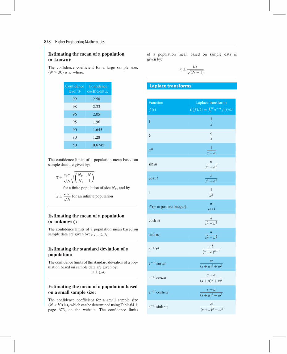
Estimating the mean of a population(σ known):

The confidence coefficient for a large sample size,(N ≥ 30) is zc where:

Confidence Confidencelevel % coefficient zc

99 2.58

98 2.33

96 2.05

95 1.96

90 1.645

80 1.28

50 0.6745

The confidence limits of a population mean based onsample data are given by:

x ± zcσ√N

√(Np − N

Np − 1

)

for a finite population of size Np , and by

x ± zcσ√N

for an infinite population

Estimating the mean of a population(σ unknown):

The confidence limits of a population mean based onsample data are given by: μx ± zcσx

Estimating the standard deviation of apopulation:

The confidence limits of the standard deviation of a pop-ulation based on sample data are given by:

s ± zcσs

Estimating the mean of a population basedon a small sample size:

The confidence coefficient for a small sample size(N<30) is tc which can be determined using Table 64.1,page 673, on the website. The confidence limits

of a population mean based on sample data isgiven by:

x ± tcs√(N − 1)

Laplace transforms

Function Laplace transforms

f (t) L{ f (t)} = ∫∞0 e−st f (t)dt

11

s

kk

s

eat 1

s − a

sin ata

s2 + a2

cosats

s2 + a2

t1

s2

tn(n = positve integer)n!

sn+1

cosh ats

s2 − a2

sinh ata

s2 − a2

e−at tn n!

(s + a)n+1

e−at sinωtω

(s + a)2 +ω2

e−at cosωts + a

(s + a)2 +ω2

e−at coshωts + a

(s + a)2 −ω2

e−at sinhωtω

(s + a)2 −ω2


The Laplace transforms of derivatives:

First derivative

L{

dydx

}

= sL{y} − y(0)

where y(0) is the value of y at x = 0

Second derivative

L{

dydx

}

= s2L{y} − sy(0)− y′(0)

where y′(0) is the value ofdy

dxat x = 0

Fourier series

If f (x) is a periodic function of period 2π then itsFourier series is given by:

f (x)= a0 +∞∑

n=1

(an cosnx + bn sin nx)

where, for the range −π to +π :

a0 = 1

2π

∫ π

−πf (x)dx

an = 1

π

∫ π

−πf (x)cosnx dx (n = 1,2,3, . . .)

bn = 1

π

∫ π

−πf (x)sin nx dx (n = 1,2,3, . . .)

If f (x) is a periodic function of period L then its Fourierseries is given by:

f (x)= a0 +∞∑

n=1

{an cos

(2πnx

L

)+ bn sin

( 2πnxL

)}

where for the range − L

2to + L

2:

a0 = 1

L

∫ L/2

−L/2f (x)dx

an = 2L

∫ L/2

−L/2f (x)cos

( 2πnxL

)dx (n = 1,2,3, . . .)

bn = 2L

∫ L/2

−L/2f (x)sin

( 2πnxL

)dx (n = 1,2,3, . . .)

Complex or exponential Fourier series:

f (x)=∞∑

n=−∞cne j 2πnx

L

where cn = 1

L

∫ L2

− L2

f (x)e− j 2πnxL dx

For even symmetry,

cn = 2

L

∫ L2

0f (x)cos

( 2πnxL

)dx

For odd symmetry,

cn = − j2

L

∫ L2

0f (x)sin

( 2πnxL

)dx

These formulae are available for downloading at the website:www.routledge.com/cw/bird

Essentialformulaes3-euw1-ap-pe-ws4-cws-documents.ri-prod.s3.amazonaws.com/... · Essentialformulae...

Documents

Transcript of Essentialformulaes3-euw1-ap-pe-ws4-cws-documents.ri-prod.s3.amazonaws.com/... · Essentialformulae...