Essays on the Economic Impacts of Climate Change … on the Economic Impacts of Climate Change on...

i

Essays on the Economic Impacts of Climate Change on

Agriculture and Adaptation

Huang Kaixing

Submitted to the University of Adelaide in partial fulfillment of the requirement for the

degree of

Doctor of Philosophy

In

Economics

June 2016

ii

Declaration

iii

Abstract

The thesis studies the potential economic impacts of climate change on agricultural production

and estimates to what extent adaptations can help to offset the potential damages of climate

change on agricultural profits. The thesis consists of three journal-style articles. Chapter 1 is the

introduction.

Chapter 2 is the article “Why do econometric studies disagree on the effect of warming on

agricultural output? A meta-analysis”. This article conducts a meta-analysis based on 130

primary econometric studies to better understand the conflict among the existing estimates of

warming on agriculture. We find that differences in the latitude of the study sample, the

temperature measure that was used, the econometric approach that was applied, and publication

biases can explain why the primary studies disagree. We also find that this disagreement can be

reduced if the primary studies use a yearly temperature measure and adopt the hedonic

modelling approach, as in doing so, they will tend to produce estimates with a similar but

previously supported view that warming will lead to positive effects on agriculture in the high

latitudes and negative effects in the low latitudes.

Chapter 3 is an article “How large is the potential economic benefit of agricultural

adaptation to climate change? Evidence from the United States”. Based on the meta-analysis of

Chapter 2, this article argues that studies of climate change impacts on agricultural profits using

panel data typically do not take account of adaptations over time by farmers, and those that do

tend to use the standard hedonic approach which is potentially biased. As an alternative, this

chapter develops a panel framework that includes farmer adaptation. When tested with United

States data, this study finds that the negative impact of expected climate change on farm profits

by 2100 is only one-third as large once likely adaptation by farmers is taken into account.

iv

Chapter 4 is the third article “The potential benefits of agricultural adaptation to warming

in China in the long run”. Based on a panel of household survey data from a large sample in

rural China, the article adopts the panel approach proposed in Chapter 3 to estimate the potential

benefits of adaptation and to identify the determinants of farmers’ adaptation capability. The

empirical results suggest that, for various model settings and climate change scenarios, long-

run adaptations should mitigate one-third to one-half of the damages of warming on crop profits

by the end of this century. These findings support the basic argument of the hedonic approach

that omitting long-run adaptations will dramatically overestimate the potential damage of

climate change. The chapter also finds that household-level capital intensity and farmland size

have significant effects on farmers’ adaptive capacities.

v

Acknowledgements

I gratefully acknowledge the constant supervision and support from my principal supervisor,

Prof. Christopher Findlay. I owe sincere thanks to my co-supervisors, Prof. Kym Anderson,

Prof. Wendy Umberger, and Dr. Jacob Wong. I am hugely indebted to my co-authors, Prof.

Jikun Huang, Prof. Jinxia Wang, and Dr. Nicholas Sim, for their invaluable efforts on the

methodology and writing of the articles included in Chapter 2 and Chapter 4.

I am very grateful to my family and friends for their support and companionship during the

past three years that I spent working on this thesis. I am forever indebted to my wife Yang Yang,

for her understanding, endless love, and unconditional support.

Finally, I thank all professional staff in the School of Economics for their heartwarming

help. The financial support from the School of Economics, University of Adelaide is gratefully

acknowledged.

vi

Contents

Essays on the Economic Impacts of Climate Change on Agriculture and Adaptation ....... i

Declaration ........................................................................................................................ ii

Abstract ............................................................................................................................ iii

Acknowledgements ........................................................................................................... v

Contents ........................................................................................................................... vi

List of Tables ................................................................................................................. viii

List of Figures .................................................................................................................. ix

Chapter 1 : Introduction .......................................................................................................... 1

1.1. The economics impacts of climate change on agriculture ......................................... 1

1.2. The extent to which adaptations help to offset climate change impacts .................... 3

1.3. The determinants of farmers’ adaptation capability .................................................. 7

Statement of Authorship for Chapter 2 ........................................................................... 10

Chapter 2 : Why Do Econometric Studies Disagree on the Effect of Warming on

Agricultural Output? A Meta-Analysis ................................................................................ 11

2.1. Introduction .............................................................................................................. 12

2.2. The meta-regression model ...................................................................................... 14

2.3. Data and the statistical analysis ............................................................................... 16

2.4. Meta-regression results ............................................................................................ 28

2.5. Conclusion ............................................................................................................... 38

2.6. Appendix: primary studies included in the meta-analysis ....................................... 39

Chapter 3 : How Large is the Potential Economic Benefit of Agricultural Adaptation to

Climate Change? Evidence from the United States ............................................................. 53

3.1. Introduction .............................................................................................................. 54

vii

3.2. Methodology and Data ............................................................................................ 61

3.3. Empirical Results ..................................................................................................... 73

3.4. Robustness Checks .................................................................................................. 80

3.5. Concluding remarks ................................................................................................. 91

3.6. Appendix .................................................................................................................. 93

Statement of Authorship for Chapter 4 ......................................................................... 106

Chapter 4 : The Potential Benefits of Agricultural Adaptation to Warming in China in the

Long Run ............................................................................................................................... 107

4.1. Introduction ............................................................................................................ 108

4.2. Data sources and summary statistics ..................................................................... 112

4.3. Conceptual framework and econometric approach ............................................... 120

4.4. Empirical results .................................................................................................... 128

4.5. Conclusions ............................................................................................................ 136

Chapter 5 : Concluding Remarks ....................................................................................... 137

5.1. Souces of the heterogeneity in the climate change impact literature ..................... 138

5.2. The extent to which US agriculture will adapt to climate change ......................... 140

5.3. Determinants of farmers’ adaptation capability in rural China ............................. 142

5.4. Policy recommendations ........................................................................................ 145

5.5. Limitation and further studies ................................................................................ 146

References ..................................................................................................................... 149

viii

List of Tables

Table 2-1: Definition of the independent variables ................................................................. 20

Table 2-2: Summary statistics of the independent variables .................................................... 21

Table 2-3: The influence of primary study characteristics on the inconsistency of the estimated

effects of warming ........................................................................................................ 30


effects of warming (sub-group regressions) ................................................................. 34

Table 3-1: Climatic variations after using different fixed effects ............................................. 64

Table 3-2 : Regression results of the effects of climatic variables on agricultural profits and

farmland values ............................................................................................................. 75

Table 3-3: Predicted end-of-this-century impact of climate change on agricultural profits and

the benefits of adaptation .............................................................................................. 78

Table 3-4: Robustness checks for the estimated impacts of climate change and the benefits of

adaptation (billions of 2012 constant dollars/year)....................................................... 86

Table 3-5: the consequences of fixed effects on the climate change impact panel study ......... 94

Table 3-6: A summary of agricultural production data .......................................................... 100

Table 3-7: Summary Statistics of Climate Normal and Climate Predictions ......................... 100

Table 4-1: Definition of variables ........................................................................................... 116

Table 4-2: Summary statistics of variables ............................................................................. 117

Table 4-3: Predicted changes in yearly climatic variables ..................................................... 119

Table 4-4: The magnitudes of inter-county climate variation and local weather shocks ....... 123

Table 4-5: Regression results of the effects of climatic variables and household characteristics

on agricultural profits.................................................................................................. 130

Table 4-6: Impacts of warming on crop profits by the end of this century and the benefits of

long-run adaptation (2010 constant USD per hectare per year) ................................. 132

ix

List of Figures

Figure 1-1: Value of land as a function of average temperature ................................................ 4

Figure 2-1: Geographic distribution of the observations .......................................................... 19

Figure 2-2: Distribution of the meta-dependent variable within each latitude quintile group . 23

Figure 2-3: Temperature measures and the estimated effects of warming ............................... 25

Figure 2-4: Publication status and the estimated effects of warming ....................................... 26

Figure 2-5: Incorporating adaptations and the estimated effects of warming .......................... 27

Figure 2-6: Biological differences and the estimated effects of warming ................................ 28

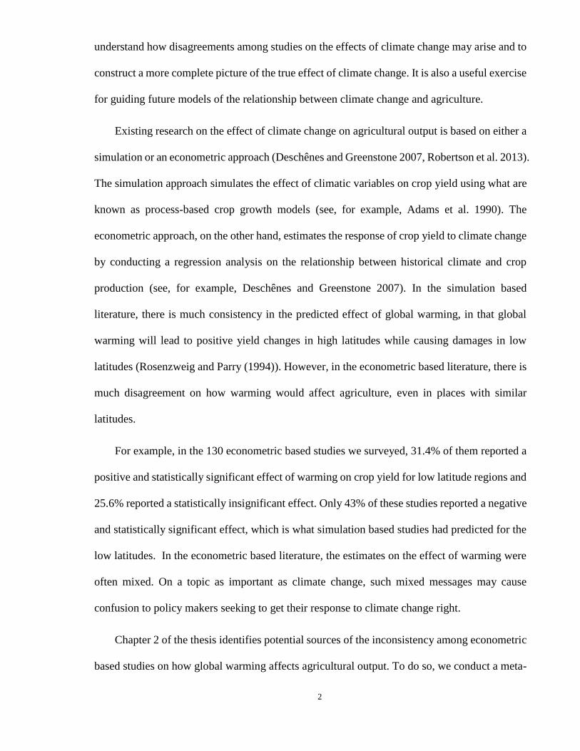
Figure 2-7: Distributions of the effects of warming within each latitude quintile group for

hedonic studies that use yearly temperature measures ................................................. 38

Figure 3-1: Predicted end-of-this-century impact of climate change on agricultural profits and

farmland rents ............................................................................................................... 77

Figure 3-2: Geographic distribution of county-level effects of climate change by the end of this

century under scenario CCSM4 RCP4.5 ...................................................................... 90

Figure 3-3: Geographic distributions of GDD and GTP for climate normal and scenario CCSM4

RCP4.5 ........................................................................................................................ 102

Figure 3-4: Yearly mean temperature fluctuations in the US, 1960–2010 ............................. 104

Figure 3-5: A simulation of farmers’ believed “true” temperature rise after an assumed 5 °C

temperature increase in the base year ......................................................................... 105

Figure 4-1: Sample provinces of the survey in China. ........................................................... 113

1

Chapter 1 : Introduction

There is a global concern that climate change could cause severe shortages in the world’s food

supply (Conway and Toenniessen 1999, Lobell and Asner 2003). To address this threat, policy

makers would benefit from robust empirical evidence on the effect that climate change has on

agricultural production. Understanding how much adaptation is likely to occur is central to any

study of the impact of climate change on agriculture and is also of paramount importance from

a policy perspective (Di Falco, Veronesi, and Yesuf 2011, Di Falco 2014). The role of adaptation

is central to the debate surrounding the impacts of climate change on agriculture. Even more

interesting from a policy perspective are the determinants of adaptation capability, because

identifying the determinants of farmers’ adaptation capabilities can support the design of

effective adaptation policies. The main purposes of this thesis are to estimate the potential

economic impacts of climate change on agriculture, to assess the extent to which adaptations

will help to offset the damages, and to identify the determinants of farmers’ adaptation

capabilities.

1.1. The economics impacts of climate change on agriculture

There is a concern across the world that climate change may lead to severe shortages in the

world’s food supply (Conway and Toenniessen 1999, Lobell and Asner 2003, Brown and Funk

2008). To address this threat, it is important for policymakers to be informed by robust empirical

evidence on the effect that global warming has on agriculture. However, in the applied

econometrics literature, there is much contention on what this effect might be or if it even exists

(see, for example, Mendelsohn, Nordhaus, & Shaw, 1994; G. C. Nelson et al., 2014; Schlenker

& Roberts, 2009). Identifying the potential sources of this dispute can enable us to better

2

understand how disagreements among studies on the effects of climate change may arise and to

construct a more complete picture of the true effect of climate change. It is also a useful exercise

for guiding future models of the relationship between climate change and agriculture.

Existing research on the effect of climate change on agricultural output is based on either a

simulation or an econometric approach (Deschênes and Greenstone 2007, Robertson et al. 2013).

The simulation approach simulates the effect of climatic variables on crop yield using what are

known as process-based crop growth models (see, for example, Adams et al. 1990). The

econometric approach, on the other hand, estimates the response of crop yield to climate change

by conducting a regression analysis on the relationship between historical climate and crop

production (see, for example, Deschênes and Greenstone 2007). In the simulation based

literature, there is much consistency in the predicted effect of global warming, in that global

warming will lead to positive yield changes in high latitudes while causing damages in low

latitudes (Rosenzweig and Parry (1994)). However, in the econometric based literature, there is

much disagreement on how warming would affect agriculture, even in places with similar

latitudes.

For example, in the 130 econometric based studies we surveyed, 31.4% of them reported a

positive and statistically significant effect of warming on crop yield for low latitude regions and

25.6% reported a statistically insignificant effect. Only 43% of these studies reported a negative

and statistically significant effect, which is what simulation based studies had predicted for the

low latitudes. In the econometric based literature, the estimates on the effect of warming were

often mixed. On a topic as important as climate change, such mixed messages may cause

confusion to policy makers seeking to get their response to climate change right.

Chapter 2 of the thesis identifies potential sources of the inconsistency among econometric

based studies on how global warming affects agricultural output. To do so, we conduct a meta-

3

analysis based on 130 primary studies, where we construct a meta-regression model that uses

their econometric estimates (of the effect of warming on agriculture) as a meta-dependent

variable and regressing it on several control variables, with each capturing a feature associated

with these studies (e.g. the geographical location on which they are based, the type of crops

studied, and the specification of the econometric model).

The meta-regression shows that 64.8% of the inconsistency among the 130 primary studies

can be explained by the differences in model specification, biological characteristics of crops,

study region and publication bias. We also find that for primary studies that have two fixed

characteristics – the use of yearly temperature and the hedonic approach – their estimates will

have less dispersion and will tend to concur with the prediction from the simulation-based

literature that warming will lead to positive effects on agriculture in high latitude regions but

damages in low latitude regions.

1.2. The extent to which adaptations help to offset climate change impacts

Understanding how much adaptation is likely to occur is central to any study of the impact of

climate change on agriculture and is also of paramount importance from the policy perspective

(Di Falco, Veronesi, and Yesuf 2011, Di Falco 2014). The role of adaptation is central to the

debate surrounding the impacts of climate change on agriculture. In an effort to avoid the

potential downward bias of the production function approach caused by omitting adaptation,

Mendelsohn, Nordhaus, and Shaw (1994) proposed a hedonic approach to identifying climate

change impacts that includes adaptations. To address the potential bias due to misspecifications

of the cross-sectional hedonic approach, Deschênes and Greenstone (2007) proposed a panel

approach to identifying climate change impacts through random inter-annual weather

fluctuations. However, because farmers can have only limited adaptations to the random year-

4

to-year weather fluctuations, the merits of this panel approach depend on how much adaptation

will actually occur in response to long-run climate change (Seo 2013).

The adaptation of agriculture to climate change is usually defined in terms of production

behavior adjustments by agricultural agents in order to moderate any negative effects or to

exploit beneficial opportunities from the changed climate (Zilberman, Zhao, and Heiman 2012,

Lobell 2014, Burke and Emerick 2015). The idea of the potential value of adaptation is usually

shown by an illustrative relationship as in Figure 1.1:

D

C

B

O

O

O

O

T2

T1

WheatWheat

Grazing

Wheat

CornL

0

L1

Wheat

Temperature

Va

lue o

f A

cti

vit

y o

n P

arcel

of

Lan

d

A

Figure 1-1: Value of land as a function of average temperature

Adapted from Mendelsohn, Nordhaus, and Shaw (1994) and Kelly, Kolstad, and Mitchell (2005)

The upper locus, shown as the heavier line, is the maximum profits from land use. Suppose

the temperature increases from 1T to 2T . If farmers adapt to this change by adjusting inputs and

managements but do not switch from wheat to corn, profits with move from A to C along

wheat’s response curve. If land use substitutions are also allowed, the profits will end up at B .

If no adaptations are made, the profits may end up at some point under the wheat response curve,

such as at D . The difference between B and D is the value of adaptation. Here, the value of

5

adaptation includes potential benefits from a full range of adaptations that could be taken by

farmers, such as adjusting inputs and managements, and switching to new varieties, crops, and

other land uses.

Empirically, numerous farm-level studies have explicitly estimated the benefits of

particular adaptation measures. For example, Kurukulasuriya and Mendelsohn (2008) examined

the benefits of crop switching as a method of adaptation; Seo and Mendelsohn (2008) provided

evidence that farmers benefit from switching among different kinds of livestock when adapting

to warming; Falco and Veronesi (2013) identified the adaptation benefit from a portfolio of

strategies, which included changing crop varieties and adopting water and soil conservation

behaviors; Huang, Wang, and Wang (2015) investigated how rice farmers benefits from

adjusting their farm-management practices in adapting to extreme weather events. The existing

farm-level adaptation studies in the literature have dramatically improved our understanding of

adaptation.

In reality, as argued by Mendelsohn, Nordhaus, and Shaw (1994), there are innumerable

potential adaptation measures that farmers could apply in response to climate change. It is nearly

impossible to capture the benefits of the full range of adaptations (as shown in Figure 1-1) by

examining only individual adaptation measures. Hence, an approach to identify the benefits of

a full range of adaptations to climate change without examining individual adaptation methods

would be valuable.

Unfortunately, an effective approach for evaluating the benefits of a full range of

adaptations has not yet been developed. Even though the hedonic approach such as that used by

Mendelsohn, Nordhaus, and Shaw (1994) implicitly includes the benefits of complete

adaptations by examining climate change impact through cross-sectional climatic differences,

it cannot be used explicitly evaluated the benefits of adaptation (Hanemann 2000). In the

6

literature, the most related method of identifying the adaptation benefit is the panel approach,

which infers adaptation benefit by comparing damages estimated from inter-annual weather

fluctuations and damages identified from long-term climate trends (Dell, Jones, and Olken 2012,

Burke and Emerick 2015). However, as shown in the conceptual framework of this chapter,

there are some potential drawbacks to examining adaptation benefits through long-term climate

trends: the historical climate trend is not large enough to predict future impacts and hence

adaptations; farmers may only partly recognize and adapt to the climate trend; and many other

concurrent trends might obscure the true effects of climate change and adaptation.

Chapter 3 of this thesis proposes an alternative approach to estimating the potential value

of a full range of adaptations. This approach depends on the basic idea that impacts identified

through cross-sectional climate differences should include the benefit of a full range of

adaptations because, as assumed in the hedonic approach, farmers should have adapted to the

climate of their regions. On the other hand, impacts identified through inter-annual weather

fluctuations will not include the adaptations to long-run climate change because farmers have

only limited ex-post adjustments in response to random year-to-year weather fluctuations, and

this short-run response is not seen as adaptation to climate change. Two types of panel model

were developed to estimate the potential impacts of climate change, one depended on cross-

sectional climate differences, and the other on inter-annual weather fluctuations. Only the

former model, namely that using cross-sectional climate differences, included the benefit of

adaptations. Hence, the differences between the predicted impacts from these two models should

reflect the value of a full range of adaptations.

This approach is combined with a panel of US county-level agricultural production and

climate data and the output of various climate models to project the potential value of

agricultural adaptation to climate change in the US. The empirical results show that, when taking

7

into account adaptations, the estimated overall damages are about 9% (or USD 3.18 billion in

2012 constant values) per year by the end of this century. If adaptations are omitted, the overall

damages are as high as 30% (or USD 10.56 billion) per year. Therefore, adaptations will help

to offset about two-thirds of the overall damages, and analysis methods omitting adaptations

can substantially overestimate the damages. These results are robust to numerous specification

checks.

1.3. The determinants of farmers’ adaptation capability

An even more interesting issue from the policy perspective is to understand the determinants of

adaptation capability, as identifying the determinants of farmers’ adaptation capability can

support the design of effective adaptation policies. Empirically, a major contribution to the field

of adaptation capability study involved the hedonic approach proposed by Mendelsohn,

Nordhaus, and Shaw (1994), which implicitly includes adaptations in its climate change impact

estimation.

On the other hand, numerous farm-level studies have explicitly estimated the benefits of


the benefits of crop-switching as a method of adaptation, whereas Seo and Mendelsohn (2008)

provided evidence that farmers benefit from switching among different kinds of livestock when

adapting to warming, and Di Falco and Veronesi (2013) identified the adaptation benefits from

a portfolio of strategies that included changing crop varieties and adopting water and soil

conservation behaviors. Even though the existing farm-level adaptation studies in the literature

have dramatically improved our understanding of adaptation, as argued by Mendelsohn,

Nordhaus, and Shaw (1994), in reality, innumerable potential adaptation measures could be

applied by farmers in response to climate change, and it is impossible to capture the benefits of

the full range of adaptations by examining only individual adaptation measures. In addition,

8

most of the farm-level studies explain the responses to weather fluctuations as adaptations, so

interpretation of these studies might have precluded some of the potential benefits of long-term

adaptation from adjusting ex ante production behaviors (Seo 2013).

However, the study of the determinants of farmers’ adaptation capability is incomplete. A

great many studies within the adaptation literature are concerned with empirically assessing

financial, informational, and institutional constraints on adaptation capacity (Kelly and Adger

2000, O'Brien, Sygna, and Haugen 2004, Parson et al. 2003). Some other studies take an

experimental or empirical approach to infer the determinants of adaptation capability under

climate change by examining farmers’ responses to extreme weather conditions or natural

disasters (See, for example, Golnaraghi and Kaul 1995, Podesta et al. 2002, Grothmann and Patt

2005, Huang, Wang, and Wang 2015). In these studies, the value of an adaptation is identified

by comparing agricultural outputs from farms that take a certain adaptation measure with the

outputs from those that do not take that adaptation measure. These studies shed important light

on the determinants of adaptation capability and generally imply that farmers with better

infrastructure, higher crop diversification, more financial and technical support, and better

information are better at adaptation. However, since they lack an explicit estimate of the value

of a full range of adaptations, previous studies do not examine the determinants of the overall

adaptation capability.

Chapter 4 of this thesis provides more empirical evidence on the determinants of farmers’

adaptation capability. Using the panel approach introduced in Chapter 3, we can explicitly

identify the potential value of a full range of adaptations, so it is possible to examine the

influencing factors of an overall adaptation capability. In our data set, complete farm and

household characteristics are included, such as the capital and labor intensity of agricultural

production and the farmers’ ages and education levels. By combining these farm and household

9

characteristics with the value of a full range of adaptations, we were able to examine the

influence of these characteristics on adaptation value and were able to gain an additional

understanding of the determinants of farmers’ adaptation capability.

10

Statement of Authorship for Chapter 2

11

Chapter 2 : Why Do Econometric Studies Disagree on the Effect

of Warming on Agricultural Output? A Meta-Analysis

Abstract

Having robust estimates of how global warming affects agriculture is important to

policymakers, but the existing econometric-based studies have been at odds on what this effect

might be. This chapter conducts a meta-analysis based on 130 primary econometric-based

studies to better understand the conflict among the existing estimates of the effect of warming

on agriculture. We find that differences in the latitude of the study sample, the temperature

measure that was used, the econometric approach that was applied, and publication biases can

explain why the primary studies disagree. We also find that this disagreement can be reduced if

the primary studies use a yearly temperature measure and adopt the hedonic modelling approach,

as in doing so, they will tend to produce estimates with a similar but previously supported view

that warming will lead to positive effects on agriculture in the high latitudes and negative effects

in the low latitudes. (JEL Q15, Q51, Q54)

Key words: Climate change impact, Agriculture, Meta-analysis, Inconsistency

12

2.1. Introduction

There is a concern across the world that climate change may lead to severe shortages in the

world’s food supply (Conway and Toenniessen 1999, Lobell and Asner 2003, Brown and Funk

2008). To address this threat, it is important for policymakers to be informed by robust

empirical evidence on the effect that global warming has on agriculture. However, in the applied

econometrics literature, there is much contention on what this effect might be or if it even exists

(see, for example, Mendelsohn, Nordhaus, and Shaw 1994, Nelson et al. 2014, Schlenker and

Roberts 2009).

In this chapter, we conduct a meta-analysis on 130 econometric-based studies to try to

understand the fundamental causes of the disagreements on the effect of warming on agriculture.

Among the 130 studies sampled here, 36.2% of them reported negative and statistically

significant marginal effects of warming, 33.2% reported positive and statistically significant

marginal effects, and the remaining 30.6% found this effect to be statistically insignificant.1 As

such, there is no consensus on the effect of warming on agriculture, which might explain why

the effect of global warming remains a greatly debated issue. To examine the fundamental

sources of this lack of consensus, we conduct a meta-analysis to help us understand why the

econometric-based literature on climate change may disagree, and in particular, if the

conclusions from such studies are dependent on the study design.

1 See the data and statistical analysis section for more details. In the summary we include both

published and unpublished primary studies. If summarize across only published studies, the shares are

31.7%, 41.4%, and 27% for studies report negative and significant, positive and significant, and

insignificant marginal effects, respectively.

13

The existing literature on the effect of global warming on agriculture are based either on a

simulation or an econometric approach (Robertson et al. 2013).2 Although there are meta-

analyses on the simulation-based studies (See, for example, Rosenzweig and Parry 1994,

Challinor et al. 2014), our study is the first to conduct a meta-analysis on the econometric-based

studies. Here, the main challenge we encounter is finding a so-called “effect-size”, which in this

context is a variable that says something about the effect of warming that is comparable across

the econometric-based studies. Having a common effect-size is crucial for enabling us to

conduct a meta-analysis to examine how the effect of warming is influenced by various features

in the econometric studies.3

To proceed, we obtain the common effect-size as the Z-values of the marginal effect of

warming on agriculture from the 130 econometric-based primary studies considered in our

meta-analysis. We then construct a meta-regression model that uses these Z-values as the meta-

dependent variable, which we regress on several independent variables capturing various

aspects of the primary studies (e.g. the geographical location, the type of crops studied, and the

specification of the econometric model). We find that a large share of the disagreement among

the primary studies can be explained by the differences in the latitude which the study is based

2 The simulation approach simulates the effect of climatic variables on crop yield using what are

known as process-based crop growth models, while the econometric approach estimates the response of

crop yield to climate change by conducting a regression analysis.

3 Since meta-analysis requires a common effect-size that is comparable among studies and this

common effect-size is not exists between the simulation study and the econometric study, it is impossible

to include both econometric and simulation studies in a single meta-analysis.

14

upon, the temperature measure used (yearly versus growing season temperature), the

econometric approach taken (hedonic versus non-hedonic models), and publication biases.

With the knowledge of how disagreements among these studies may arise, we then

investigate to what extent the dispersion in the primary estimates can be reduced if the

characteristics of the primary studies are fixed along certain dimensions. We find that for

primary studies that have two fixed characteristics – the use of yearly temperature and the

hedonic approach – their estimates will have less dispersion and will tend to concur with the

prediction from the simulation-based literature that warming will lead to positive effects on

agriculture in high latitude regions but damages in low latitude regions.4

For the remainder of the chapter, Section 2.2 introduces the meta-analysis approach that is

used in this chapter, Section 2.3 discusses the data and variables, Section 2.4 presents the meta-

regression results, and Section 2.5 concludes.

2.2. The meta-regression model

Meta-analysis is a method that uses the results from a pool of existing empirical studies that

seek to answer a common question on a given topic. It enjoys widespread use in economics

since the 1990s, such as in the area of environmental and resource economics (Nelson and

Kennedy 2009), international trade (Disdier and Head 2008), fiscal policy (Gechert 2015), and

foreign direct investments (Iršová and Havránek 2013), where the conclusions in the empirical

literature vary substantially. Meta-regression analysis is the most frequently used meta-analysis

4 It is worth to stress that this sub-group exercise is only used to illustrate the importance of these

factors in determining the observed inconsistency among primary studies, and we do not suggest that

studies with these characteristics are more reliable than other studies.

15

technique in economics. One of the main purposes of meta-regression is to identify features in

the research design that are responsible for the variation among reported empirical estimates on

the same topic (Stanley and Jarrell 1989, Smith and Huang 1995, Klomp and De Haan 2010).

In a meta-regression analysis, the dependent variable is sometimes known as the “effect size,”

which is a quantifiable result of the primary studies covered in the meta-analysis. The effect-

size can be the regression coefficient, marginal effect, elasticity, T-value, Z-value, significance

level of a coefficient, or other measures that are comparable across studies (Nelson and Kennedy

2009). The chosen effect-size for the meta-regression must be measuring the same thing as it

will be used to construct the meta-dependent variable (Stanley and Jarrell 1989).

In this study, the chosen effect-size (called meta-dependent variable hereinafter) is the Z-

value of the estimated marginal effect of warming on agricultural output or profits from the

primary study.5 There are two advantages in using the Z-value over the estimated marginal

effect itself. Firstly, the Z-value, unlike the marginal effect, has been normalized by the standard

error, which reduces heteroscedasticity (Card and Krueger 1995, Becker and Wu 2007).

Secondly, the Z-value is truly comparable across studies, unlike the marginal effect and

regression coefficient which are usually incomparable as they depend on how the regressor of

interest is defined (e.g. different units).6

5 We focus on the marginal effect of temperature for two reasons. First, warming is the most

important characteristic of climate change (IPCC, 2007). Second, the estimated marginal effects of

precipitation is less reliable because precipitation is not a good measure of water supply for crops grown,

especially for the irrigated agriculture (Schlenker, Hanemann, and Fisher 2005)

6 More detailed definition of the meta-dependent variable is provided in the next section.

16

The independent variables capture the various characteristics of the primary studies (e.g. the

geographical location where they are based on, the type of crops studied, and the specification

of the econometric model). Let iZ be the Z-value of the marginal effect of warming from primary

study i . Our meta-regression model is

0

1

1,2,...ik ii

ki i

K

k

i

Xi L

se s seZ

e

(2.1)

where ise is the standard error of the marginal effect from study i, ikX is a K-vector of

characteristics of the primary studies; 𝛼0 is a constant term of the regression; 𝛼𝑘 is the meta-

regression coefficient on the kth independent variable, and this captures the influence that the kth

study characteristic has on the heterogeneity across primary studies (Bel, Fageda, and Warner

2010); 𝜇𝑖 captures the remaining variation in iZ beyond the study characteristics under

consideration. As a clarifying remark, climate change impact studies are usually conducted with

large samples. As such, the standardized marginal effect of warming can be approximated

reasonably well by the standard normal distribution. For this reason, we refer to this

standardized marginal effect as the Z-value instead of the T-value.

2.3. Data and the statistical analysis

To perform a good meta-analysis, it is important to cover the literature as widely and as

comprehensively as possible (Cavlovic et al. 2000). We carried out a broad and inclusive search

of the rapidly growing econometric-based literature that examines the effect of climate change

on agricultural output. We searched the related published and unpublished studies from a variety

of sources. For published papers, we looked up the Web of Science, Google Scholar, Academic

OneFile, Academic Search Premier, JSTOR, and Scopus, as well as the websites of major

17

publishers of academic journals, including Springer, Elsevier, Emerald, Blackwell, and Wiley.

For unpublished papers (e.g. working papers, government reports, and dissertations), we

searched Google Scholar, SSRN, websites of renowned research institutes, and the websites of

major government agencies. In all, our search took about nine months (July 2014 - March 2015)

and covered more than 1000 papers, of which we selected 130 papers based on the following

criteria.

First, the papers must contain some econometric analysis; studies that were purely

simulation based were excluded.7 Second, they must focus on the effects of warming on the

yield or profits of four major crops (maize, soybean, wheat and rice), on farmland values, or on

agricultural profits. Third, the papers must provide enough information for us to obtain the

marginal effect of warming evaluated at the mean temperature; studies that reported solely the

effects of extreme temperatures, such as the effects of minimum and maximum temperature,

were excluded. The temperature can be measured by yearly average temperature, yearly degree-

day, growing season average temperature, or growing season degree-day. Finally, the papers

must contain enough information for us to obtain or construct the Z-value pertaining to the

marginal effect of warming on agriculture.

Even though several selection criteria were applied, the marginal effects of warming from

the chosen primary studies are still not perfectly comparable for several reasons. Firstly, the

dependent variable in the primary studies may be defined differently. For example, it could be

the yield or profits of one, several or all crops, the agricultural profits, or the farmland value.

Secondly, different measures of temperature (as an indicator of warming) may be adopted by

different primary studies. For example, some studies adopted yearly or growing season average

7 See footnote 3 for why we exclude simulation studies.

18

temperature as their temperature measure, others adopted yearly or growing season degree-day.

Thirdly, the way these primary studies are conducted may vary across countries, especially in

the use of different units for the dependent variable or the independent variables.

To make a reasonable comparison among the papers chosen for our meta-analysis, we will

focus on the Z-value of the marginal effect of warming evaluated at the mean temperature. This

Z-value tells us if an increase in temperature around its mean has a statistically significant and

positive or a statistically significant and negative effect on agricultural output, or if this effect

is statistically insignificant. Because it is a standardized statistic, it conveys information about

the effect of warming on agriculture in a consistent way across the primary studies, unlike the

regression coefficient on temperature which is generally not comparable. However, from a

hypothesis testing perspective, the magnitude of the Z-value is meaningful only when compared

with the threshold Z-value that stands for a particular significance level. Hence, we classify the

Z-value as positive and significant if it is above 1.68, negative and significant if it is below -

1.68, and insignificant otherwise.8 As such, our study will focus on the direction of the marginal

effect of warming and the significance level of this marginal effect evaluated at the mean

temperature.9

8 The critical Z-value of ±1.68 corresponds to a 10% significance level in the large sample climate

change impact studies. We also tried to use the critical values that correspond to 5% or 1% significance

levels, and the major conclusions of this study keep the same.

9 We do not compare the estimated future impacts of warming across different studies. This is

because different climate change scenarios are usually used, which make the estimated future impacts

generally incomparable.

19

Figure 2-1: Geographic distribution of the observations

From the 130 papers, we constructed a dataset with 341 observations, which is the total

number of estimates of the effect of warming on agriculture contained in these papers. If there

are multiple estimates involving the same crop, profit, or farmland value in a primary study, we

pick only one estimate for each of these from the primary study to avoid the problem of non-

independence among observations on the effect-size.10 The observations exceed the number of

paper collected because each paper often reports estimates associated with several different

crops. Figure 2-1 presents the geographic distribution of the observations, which are drawn from

36 countries and 103 locations. 27% of our sample is associated with studies on Africa, 22% on

10 Estimates within one primary study may not be independent of each other. Including correlated

effect-size estimates will result in biased standard error estimates in the meta-regression (Nelson and

Kennedy 2009). Therefore, if there are multiple estimates involving the same crop, we will only choose

one.

20

the United States, 21% on China, 7% on India, 6% on the European Union, and 17% for the rest

of the world.

Table 2-1: Definition of the independent variables

Independent variables Definition

Regional differences

(1) Latitude Mean latitude of the study area (Degree) §

Model specification

(2) Measures of output Agricultural output is measured by profits or quantity (1 =

Profits , 0 = Quantity)

(3) Temperature measures Using a yearly temperature measure or a growing season

temperature measure (1 = Yearly, 0 = Growing season) †

(4) Control for irrigation Did the primary study control for irrigation (1 =Yes, 0 = No)

Publication bias

(5) Research time Year of study (Year)

(6) Publication status Published (in journal or book) or not (1 = Yes, 0 = No)

Including adaptation

(7) Adaptation Depending on the hedonic approach or not (1 = Yes, 0 = No)

Biological differences

(8) Crop types Maize, soybean, wheat, rice, agricultural profits, or farmland

value (0 = farmland values, farmland rents or agricultural profits,

1 = Maize, 2 = Soybean, 3 = Wheat, 4 = Rice)#

§: We do not make a distinction between the latitude of Southern and Northern Hemisphere. For

example, 23.43° N is treated the same as 23.43° S.

†: The yearly temperature measure includes yearly mean temperature and yearly degree-day; the

growing season temperature measure contains growing season mean temperature and growing season

degree-day.

#: Maize, soybean, wheat and rice are the most frequently studied crops. There are also lots of

econometric studies examined the effect of warming on farmland rents, farmland values, and

agricultural profits, which reflect the effect of warming on the combination of various crops and other

farmland uses.

21

From each of these 341 observations, we gathered 8 study characteristics that we believe

have the potential to explain the disagreement among the primary studies. These characteristics

will be quantified and used as independent variables. Table 2-1 provides the definitions of the

study characteristics, which are grouped into five categories: regional differences, model

specification, publication bias, adaptation, and biological differences. The summary statistics of

independent variables are presented in Table 2-2.

Table 2-2: Summary statistics of the independent variables

Panel A: Continuous variables Mean Standard

Deviation Min Max

Latitude (Degrees) 30.07 14.80 0.005 64.32

Research time (Year) 2010 4 1992 2015

Panel B: Discrete variables Variable

= 1

Variable

= 0

Measure of output (1 = Profits, 0 = Quantity) 145 196

Temperature measures (1 = Yearly, 0 = Growing season) 232 109

Adaptation (1=Hedonic approach, 0=others) 148 193

Control for irrigation (1 = Yes, 0 = No) 41 300

Publication status (1 = Published, 0 = Unpublished) 235 106

Maize (1 = Yes, 0 = No) 70 271

Soybean (1 = Yes, 0 = No) 23 318

Wheat (1 = Yes, 0 = No) 42 299

Rice (1 = Yes, 0 = No) 53 287

Land values, land rents or agricultural profits (1 = Yes, 0 = No) 152 189

Number of observations 341

Note: the definition of independent variables can be found in Table 2-1.

The latitude is an important factor for how warming may influence agricultural production.

To show this, we distribute the 341 observations evenly into five groups according to the

latitudes associated with these observations. The low latitude group is defined as the first 20%

22

of observations nearest to the equator (either from the Southern or Northern Hemisphere). The

low-middle latitude group is defined as the next 20% of observations nearest to the equator, and

so on.

Figure 2-2 summarizes the meta-dependent variable corresponding to each of these five

latitudes groups, and show that the latitude of the region where a study is based on may explain

a significant share of the disagreement of the effects of warming among the primary studies.

This is because the marginal effects of warming on agricultural output may vary depending on

crop type, which in turn depends on regional gradients of temperature (Cramer and Solomon

1993, Ramankutty et al. 2002). From the existing meta-analyses of the simulation-based

literature, we are now aware that warming mainly has negative effects on agricultural production

in low latitudes and positive effects in high latitudes (Rosenzweig and Parry 1994, Challinor et

al. 2014). However, as shown in Figure 2-2, even the econometric estimates of the effect of

warming (i.e. the Z-value of the marginal effect) from studies in the same latitude region can be

highly mixed.

23

Figure 2-2: Distribution of the meta-dependent variable within each latitude quintile group

Note: This figure shows the percentage of observations reporting (i) positive and significant effects of

warming, (ii) insignificant effects, (iii) negative and significant effects (all at the 10% significance level)

for each of the five sample latitude quintile groups. The Low quintile group contains the first 20% of

observations nearest to the equator, the Low-Middle quintile group contains the next 20% of observations

nearest to the equator, and so on.

For example, among studies corresponding to the low latitude regions, as indicated by the

Low group in Figure 2-2, 31.9% of the estimates show that warming has a positive and

statistically significant marginal effect (at the 10% level), 21.7% of the estimates are statistically

insignificant, and 46.4% of the marginal effects are negative and statistically significant. Such

disparity can also be found among studies within each of the other four latitude groups. That

being said, from Figure 2-2, there appears to be a relationship between the extent of the

disagreement among the primary studies and the latitude in which the studies are based on. For

example, the share of studies that reported positive and significant marginal effects increases

24

with latitude. At the same time, the share of studies that reported negative and significant effects

decreases with latitude.

Differences in the temperature measure could be an important reason for why the primary

studies disagree on the effects of warming. In the econometric-based literature, temperature is

usually measured either as yearly temperature (includes yearly mean temperature and yearly degree-

day) or as growing season temperature (includes growing season mean temperature and growing

season degree-day). However, this distinction is not trivial. Figure 2-3 shows that the differences

in how temperature is measured can result in substantial disagreement about the effects of

warming. For example, the share of studies that reported statistically significant and positive

effects are much larger for studies using a yearly temperature measure than studies using a

growing season temperature measure (Panel C in Figure 2-3).

The sensitivity of the effects of warming to the way in which temperature is measured could

be due to the fact that different measures of temperature (i.e. yearly or growing season) capture

different things. For example, the temperature affects crops mainly through the growing season

during which crops are on the field. Therefore, the growing season temperature is a more

relevant measure of temperature to study its effect on crops. However, the downside of using it

is the difficulty in identifying the growing season because in certain areas, crops are grown

throughout the year. While the yearly temperature is not as tightly linked to the growing season,

it has the advantage of capturing such adaptations by farmers when farmers switch growing

seasons in response to warming (Kurukulasuriya and Mendelsohn 2008).

25

Figure 2-3: Temperature measures and the estimated effects of warming

Note: The yearly temperature measure includes yearly mean temperature and yearly degree-day;

the growing season temperature measure contains growing season mean temperature and growing

season degree-day.

Another possible source of disagreement is publication bias. Generally, there is evidence of

publication bias in applied econometric research, as results that conform to prevailing views are

more likely to be published (Rosenthal 1979). To capture the notion of publication bias, we

consider the publication status (published or unpublished) and publication year of the primary

studies as independent variables.

In the context of the global warming literature, Figure 2-4 shows that studies that reported

negative effects of warming were more likely to be published than studies that reported positive

effects. Our reading of the literature is that in the early stage of the climate change impact study,

the publications tend to be related to research that reported dramatic negative effects of warming,

which affirmed the view that warming was damaging to agriculture. However, the recent years

have seen an increasing number of publications that reported mild negative effects or even

26

positive effects of warming. That being said, Figure 2-4 demonstrates that studies showing

favorable effects of warming are still more unlikely to be published than those showing either

no effects or unfavorable effects of warming.

Figure 2-4: Publication status and the estimated effects of warming

Long-run adaptations can help farmers to exploit future benefits of climate change on

agriculture or mitigate its future negative impact (Lobell et al. 2008). Here, the primary studies

differ on whether long-run adaptations are accommodated in the design of their econometric

analysis. In the literature, the hedonic approach developed by Mendelsohn, Nordhaus, and Shaw

(1994) is the most common approach for capturing adaptations when estimating the impact of

climate change. In this approach, the possibility of long-run adaptations is reflected by the cross-

sectional differences in climate and agricultural output. The intuition is that over the long run,

it is reasonable to assume that agricultural agents would have completely adapted to the climate

of their particular regions. Therefore, the persistent regional difference in agricultural output

would contain information about long-run adaptations by agricultural agents to their local

climate.

27

Besides the hedonic approach, which looks mainly at the between-region effects of

temperature on agricultural output, there are econometric models of climate change that exploit

mainly the within-region effects of weather, whose variation comes from inter-annual weather

fluctuations (Deschênes and Greenstone 2007). Impacts of warming identified through inter-

annual weather fluctuations do not include the benefits of long-run adaptations as farmers

typically make very limited ex post adjustments to random weather outcomes (Seo 2013).

Consequently, compared with studies based on the hedonic approach, studies based on inter-

annual weather fluctuations tend to understate the benefits of warming as they do not account

for long-run adaptations. From Figure 2-5, we find some evidence to support this conjecture, as

among studies that reported significant and positive effects of warming, the proportion of

hedonic-based studies exceeds the proportion of the other types of studies by 14.1 percentage

points. This implies that studies based on the hedonic approach (which takes into account of

long-run adaptations) tend to have a more positive view about warming.

Figure 2-5: Incorporating adaptations and the estimated effects of warming

Note: Studies using the hedonic approach incorporate more long-run adaptations than studies

using other approaches (Mendelsohn et al. 2004).

28

Finally, the biological difference among crops may explain why the primary studies disagree.

In the climate change literature, there are four widely studied crops: maize, soybean, wheat, and

rice. However, as shown in Figure 2-6, the estimated effect of warming on crops is dependent

on the type of crops. For example, 78.3% of the primary studies on soybean reported positive

effects while this is true for only 22.2% of the primary studies on rice. In other words, a positive

effect of warming is more likely to be observed if the crop in question is soybean. However, the

opposite is true if a study focuses on rice.

Figure 2-6: Biological differences and the estimated effects of warming

2.4. Meta-regression results

In this section, we report the meta-regression results that demonstrate to what extent the

disagreement among the primary studies on the effect of warming on agriculture can be

explained by the study characteristics that we have discussed. The meta-dependent variable of

interest is Z-value pertaining to the marginal effect of warming evaluated at the mean

29

temperature that are either reported by the primary studies or constructed by us from the

information available in these studies. The definitions of the independent variables, each of

which pertain to a specific study characteristic, can be found in Table 2-1.

Table 2-3 reports our regression results based on the estimation of eq. (2.1). Column (1)

reports the baseline result that is obtained from estimating eq. (2.1) with the full sample. In

Columns (2)-(4), we omit studies from various regions as a sensitivity check, where Column (2)

excludes China, Column (3) excludes Africa, and Column (4) excludes the United States. These

three regions are the most extensively studied regions among the primary studies in our sample.

Across Columns (1)-(4), the influence of the independent variables on the Z-value is quite

consistent in terms of the direction of influence, magnitude, and statistical significance. This

implies that our meta-regression results are not overly dependent on the regional composition

of the primary studies used in this meta-analysis. The independent variables explain a significant

proportion of the variation in the primary estimates (as expressed by the Z-values). For the full

sample regression in Column (1), the adjusted R2 of 56.28% indicates that the independent

variables account for 56.28% of the variation in the primary estimates. For the sub-sample

regressions across Columns (2)-(4), the adjusted R2 ranges from 46% to 60.34%.

30


effects of warming

Independent variable

(1) Full

Model

(2) Exclude

China

(3) Exclude

Africa

(4) Exclude the

United States

Regional differences Latitude (Degree) 0.03*** 0.03*** 0.02*** 0.02***

(0.00) (0.00) (0.01) (0.00) Model specification

Measures of output (1 = Profits , 0 = Quantity)

0.29* 0.25 0.60** 0.24 (0.15) (0.16) (0.28) (0.18)

Temperature measures (1 =

Yearly, 0 = Growing season) 0.38*** 0.39*** 0.34*** 0.47***

(0.10) (0.11) (0.12) (0.13)

Control for irrigation

(1 = Yes, 0 = No)

-0.15 -0.13 -0.22 -0.13

(0.16) (0.19) (0.18) (0.26)

Publication bias

Research time 0.03** 0.03** 0.03** 0.02 (Year) (0.01) (0.01) (0.01) (0.02)

Publication status (1 = Yes, 0 = No)

-0.80*** -0.91*** -0.75*** -0.63*** (0.10) (0.12) (0.12) (0.13)

Including adaptation Adaptation (1=Hedonic approach, 0=others)

0.46*** 0.60*** 0.74*** 0.47*** (0.15) (0.17) (0.22) (0.17)

Biological differences Maize (1 = Yes, 0 = No)

0.58*** 0.61*** 0.50** 0.60*** (0.15) (0.19) (0.23) (0.20)

Soybean (1 = Yes, 0 = No)

0.97*** 1.03*** 0.86*** 1.11*** (0.19) (0.23) (0.26) (0.25)

Rice (1 = Yes, 0 = No)

0.72*** 0.90*** 0.56** 0.66*** (0.18) (0.26) (0.24) (0.23)

Wheat (1 = Yes, 0 = No)

0.17 0.49** 0.03 0.14 (0.17) (0.21) (0.24) (0.21)

Constant -59.10** -59.80** -71.26** -39.11

(25.89) (28.53) (29.26) (34.90) Observations 341 270 251 265 Adjusted R2 56.28% 60.34% 50.26% 46.00%

Notes: The Huber-White heteroskedastic-consistent standard errors are reported in parentheses.

Significance levels are *** p<0.01, ** p<0.05, * p<0.1. The definition of moderator variable is in Table

2-1.

From Table 2-3, we can gather some insights into why the estimated marginal effects of

warming may vary across studies. The first major source of the disagreement among these

31

studies comes from differences in where the primary studies are based on. For example, across

the four regressions presented in Table 2-3, the coefficients on latitude are all positive and

statistically significant, which imply that studies based on higher latitude regions are more likely

to report positive effects of warming than studies based on lower latitude regions. This result is

quite intuitive considering that the temperature in the low latitudes is much higher than that in

the high latitudes and that the productivity response of crops to temperature is first increasing

and then decreasing with temperature (Mendelsohn, Nordhaus, and Shaw 1994, Schlenker and

Roberts 2009).

The second major source of the disagreement comes from differences in model

specifications. For example, the positive and statistically significant coefficient on temperature

measure (which is a dummy variable) in the meta-regression implies that primary studies using

yearly temperature measures are more likely to report positive effects of warming than studies

using growing season temperature measures. As discussed, the yearly temperature rather than

the growing season temperature would be a more appropriate measure of temperature in view

of adaptations, as farmers could switch to a growing season that differs from the one assumed

in the growing season temperature measure (Kurukulasuriya and Mendelsohn 2008).

The third major source of the disagreement comes from publication bias. The coefficient on

publication status in the meta-regression is negative and statistically significant, which implies

that research that reported negative effects of warming were more likely to be published in

books or journals. The positive coefficient on research time also suggests that studies belonging

to a more recent vintage reported positive effects more frequently than earlier studies did. If

these recent studies (which reported positive effects) were carried out with improved

methodologies, the finding that they are less likely to be published than studies reporting

negative effects suggests that publication bias is likely to be present. This bias is further

32

supported when we run a meta-regression using only the sample of studies after 2010, which

controls for vintage, and find that the coefficient for publication status is still negative and

statistically significant.11

The forth major source of the disagreement comes from whether or not adaptation is

captured in the paper’s econometric design. In reality, farmers are likely to take adaptation

measures to moderate any negative effect of climate change or to even exploit any beneficial

opportunity that arise from warming. As such, econometric analyses that omit the adaptation by

farmers could overestimate the damages or underestimate the benefits of warming. This

argument is supported by the positive and statistically significant coefficient on adaptation,

which suggests that the primary studies that take adaptation into account (i.e. through the

hedonic modelling approach) tend to report Z-values that are either less negative or more

positive than the Z-values from studies that do not.

Finally, the primary studies may disagree on what the effect of warming might be if they

focus on different crops, which may respond to warming differently. As shown under the

“Biological Differences” category, the statistically significant coefficients on the dummies for

maize, soybean, and rice but not wheat imply that the response to warming may vary across

crops.

For our sensitivity analysis, we examine if our full sample baseline meta-regression result

(see Column (1) of Table 2-3) could be attributed to specific subsamples. In Column (1a) of

Table 2-4, we restrict our sample to the set of primary estimates that considered the response of

agricultural production as a whole, which is measured by agricultural profits or farmland values.

By contrast, in Column (1b), we consider the subsample of primary estimates that focused only

11 The result is available upon request.

33

on the response from the four major crops but not from agricultural production as a whole. In

Columns (2a) and (2b), we consider the subsample of primary estimates that measure

agricultural outputs based on quantities (Column 2a) or on profits and farmland values (Column

2b). In Columns (3a) and (3b), we consider the subsample of published primary studies (Column

3a) or unpublished primary studies (Column 3b). In Columns (4a) and (4b), we consider the

subsample that uses the hedonic approach (Column 4a) or other non-hedonic approaches

(Columns 4b).

Across the eight meta-regressions in Table 2-4 (Columns 1a-4b), we find very similar

conclusions about what the key drivers of the disagreement among the primary studies are. Just

as in Table 2-3, we find that all the coefficients on latitude and temperature measures across

Columns (1a)-(4b) in Table 2-4 are positive and statistically significant. The coefficients on

publication status are positive and statistically significant for most of the subsample meta-

regressions; the only exception is with the subsample of studies employing the hedonic approach

(Column 4a), where publication status is statistically insignificant. In our view, one possible

explanation for why hedonic-based studies are not influenced by publication bias is because

they have a good argument for the positive effects of warming (i.e., adaptations will help to

offset the negative effects).

34


effects of warming (sub-group regressions)


(1a) (1b) (2a) (2b)

All

agricultural

products

Four major

crops

Quantity of

output Profits and

farmland

values Regional differences

Latitude (Degree) 0.01* 0.03*** 0.01* 0.03***



0.47 0.40* - - (0.33) (0.23)


Yearly, 0 = Growing

season)

0.89*** 0.29** 0.43*** 0.29**

(0.22) (0.12) (0.15) (0.12)


(1 = Yes, 0 = No)

-0.41 -0.11 -0.12 -0.17

(0.26) (0.22) (0.24) (0.18)

Publication bias

Research time 0.01 0.03* 0.09*** 0.02 (Year) (0.04) (0.02) (0.03) (0.02)


-1.09*** -0.74*** -0.75*** -0.81*** (0.29) (0.12) (0.18) (0.12)

Including adaptation Adaptation (1=Hedonic approach,

0=others)

0.53** 0.70*** 1.00*** 0.26 (0.21) (0.25) (0.14) (0.24)


- -0.35** 0.26** 0.51**

(0.15) (0.13) (0.23) Soybean (1 = Yes, 0 = No)

- -0.21 0.19 0.68***

(0.19) (0.84) (0.23) Rice (1 = Yes, 0 = No)

- -0.83*** -0.71* 0.10

(0.17) (0.37) (0.23) Wheat (1 = Yes, 0 = No)

- - 0.29 0.85***

(0.58) (0.26)

Constant -25.41 -58.71* -190.32*** -36.81




2-1.

35

Table 2-4 (continue): The influence of primary study characteristics on the inconsistency of

the estimated effects of warming (sub-group regressions)


(3a) (3b) (4a) (4b)

Published Unpublished Hedonic

approach Other

approaches Regional differences

Latitude (Degree) 0.02*** 0.04*** 0.02*** 0.03***



0.23 0.67** 0.52 0.51*** (0.19) (0.31) (0.34) (0.19)


Yearly, 0 = Growing

season)

0.49*** 0.40*** 0.96*** 0.31***

(0.14) (0.14) (0.28) (0.11)


(1 = Yes, 0 = No)

0.03 -0.47** -0.00 -0.41**

(0.26) (0.18) (0.41) (0.18)

Publication bias

Research time 0.03** 0.03 -0.01 0.05*** (Year) (0.02) (0.03) (0.04) (0.02)


- - -0.79 -0.81***

(0.56) (0.11)

Including adaptation Adaptation (1=Hedonic approach,

0=others)

0.63*** 0.02 - - (0.21) (0.27)


0.54** 0.26 0.57 0.36** (0.21) (0.30) (0.49) (0.18)

Soybean (1 = Yes, 0 = No)

1.27*** 0.38 0.47 0.68*** (0.30) (0.32) (0.79) (0.22)

Rice (1 = Yes, 0 = No)

0.93*** -0.61 1.24 0.47** (0.23) (0.51) (0.90) (0.21)

Wheat (1 = Yes, 0 = No)

0.55** -0.66** -0.09 -0.13 (0.22) (0.33) (0.46) (0.21)

Constant -64.77** -55.22 28.93 -101.20***




2-1.

36

Besides publication status, the coefficients on adaptation are generally positive and

statistically significant, except in Columns (2b) and (3b) where the estimates are statistically

insignificant. With respect to the statistical insignificance of adaptation in Column (2b), the

intuition is that studies based on farmland values rely mainly on the hedonic approach.12 Given

that the hedonic approach already takes into account of adaptation, it may not be surprising that

the coefficient on adaptation is statistically insignificant in this instance. With respect to

Column (3b), which looks at the subsample of unpublished papers, the statistical insignificance

of adaptation suggests that the disagreement among the unpublished studies is not attributed to

whether or not adaptation is captured.

The various meta-regressions suggest that a large share of the disagreement among the

primary studies can be explained by differences in the latitudes which the studies are based on,

the measure of temperature (a yearly temperature versus a growing season temperature), the

modelling approach (hedonic versus other approaches), and publication bias. Therefore, as an

exercise, we investigate to what extent the dispersion in the primary estimates can be reduced if

the characteristics of the primary studies are fixed according to latitudes, temperature measure

and the modelling approach. Because of the large permutation of these characteristics, we fix

the temperature measure to yearly temperature, the modelling approach to the hedonic approach,

but allow the latitudes to vary. The motivation of choosing the yearly temperature measure

rather than the growing season temperature measure is to accommodate potential adaptations of

switching growing season in response to warming (Kurukulasuriya and Mendelsohn 2008). In

12 Most of the hedonic studies use farmland values or agricultural profits as the dependent variable,

but there are also some hedonic studies using the profits of a specific major crop as the dependent variable.

37

addition, the hedonic approach is better than other econometric approaches in incorporating

adaptations as discussed (Seo 2013).

For variations in latitudes, we again sort the studies into five latitude quintile groups: low

latitudes, low middle latitudes, middle latitudes, upper-middle latitudes, and high latitudes.

Compared with Figure 2-2 where the study characteristics are not fixed, Figure 2-7 shows that

the primary estimates from studies within the same latitudes will have less dispersion if they all

employ the yearly temperature measure and the hedonic approach. Interestingly, if we condition

our studies on having these two characteristics, we will observe the conclusion that global

warming mainly has positive effects on agriculture in the high latitudes and negative effects in

the low latitudes. This is the same conclusion made by several meta-analyses on the simulation-

based studies on climate change (Rosenzweig and Parry 1994, Challinor et al. 2014). As a caveat,

what this exercise shows is that primary studies that use measures of yearly temperature and the

hedonic approach will tend to agree with each other, conditioning on the latitudes that they are

based on. This exercise does not suggest that studies with these two characteristics are more

reliable than those without them.

38

Figure 2-7: Distributions of the effects of warming within each latitude quintile group for

hedonic studies that use yearly temperature measures

Note: This figure shows the percentage of observations reporting (i) positive and significant

effects of warming, (ii) insignificant effects, (iii) negative and significant effects (all at the 10%

significance level) for each of the five sample latitude quintile groups. The Low quintile group

contains the first 20% of observations nearest to the equator, the Low-Middle quintile group

contains the next 20% of observations nearest to the equator, and so on.

2.5. Conclusion

Having a good understanding of the relationship between global warming and agricultural

production can help policy makers to better anticipate issues concerning food security. However,

although there is a growing econometric based literature on this topic, there is also much

disagreement on what the effect of warming is, in particular, whether it is positive or negative,

or if there is an effect at all.

39

Employing a meta-analysis, this article identifies some potential sources of disagreement

among 130 primary studies. Our meta-regression results suggest that differences in the latitude

of the study sample, the temperature measure that was used, the econometric approach that was

implemented, and publication bias can explain why the primary estimates differ. We also find

that if the primary studies use the yearly temperature measure and adopt the hedonic modelling

approach, their estimates will have less dispersion and will tend to concur with the prediction

from the simulation-based literature that warming will lead to positive effects on agriculture in

the high latitudes but damages in the low latitudes.

2.6. Appendix: primary studies included in the meta-analysis

Ahmed, S. A., Diffenbaugh, N. S., Hertel, T. W., Lobell, D. B., Ramankutty, N., Rios, A. R., &

Rowhani, P. (2011). Climate volatility and poverty vulnerability in Tanzania. Global

environmental change, 21(1), 46-55.

Ajetomobi, J. O., Abiodun, A., & Hassan, R. (2011). Impacts of climate change on rice

agriculture in Nigeria. Tropical and Subtropical Agroecosystems, 14(2), 613-622.

Akpalu, W., Hassan, R. M., & Ringler, C. (2008). Climate variability and maize yield in South

Africa. Environment and Production Technology Division. IFPRI Paper, 843.

Almaraz, J. J., Mabood, F., Zhou, X., Gregorich, E. G., & Smith, D. L. (2008). Climate change,

weather variability and corn yield at a higher latitude locale: Southwestern Quebec.

Climatic change, 88(2), 187-197.

Amiraslany, A. (2010). The impact of climate change on Canadian agriculture: a Ricardian

approach. University of Saskatchewan working paper.

40

Attavanich, W., & McCarl, B. A. (2011). The effect of climate change, CO2 fertilization, and

crop production technology on crop yields and its economic implications on market

outcomes and welfare distribution. Paper presented at the Selected Paper prepared for

presentation at the Agricultural and Applied Economics Association’s Annual Meeting,

Pittsburgh, PA.

Auffhammer, M., Ramanathan, V., & Vincent, J. R. (2012). Climate change, the monsoon, and

rice yield in India. Climatic change, 111(2), 411-424.

Barnwal, P., & Kotani, K. (2010). Impact of variation in climatic factors on crop yield: A case

of rice crop in Andhra Pradesh, India. Economics and Management series.

Barnwal, P., & Kotani, K. (2013). Climatic impacts across agricultural crop yield distributions:

An application of quantile regression on rice crops in Andhra Pradesh, India. Ecological

Economics, 87, 95-109.

Benhin, J. K. (2006). Climate change and South African agriculture: Impacts and adaptation

options. Pretoria: The Centre for Environmental Economics and Policy in Africa,

University of Pretoria.

Benhin, J. K. (2008). South African crop farming and climate change: An economic assessment

of impacts. Global environmental change, 18(4), 666-678.

Blanc, É. (2012). The Impact of Climate Change on Crop Yields in Sub-Saharan Africa.

American Journal of Climate Change, 1(1), 1-13.

Blignaut, J., Ueckermann, L., & Aronson, J. (2009). Agriculture production's sensitivity to

changes in climate in South Africa. South African Journal of Science, 105(1 & 2), 61-

68.

Bootsma, A., Gameda, S., & McKenney, D. (2005). Potential impacts of climate change on corn,

soybeans and barley yields in Atlantic Canada. Canadian journal of soil science, 85(2),

345-357.

41

Boubacar, I. (2010). The effects of drought on crop yields and yield variability in Sahel. Paper

presented at the The Southern Agricultural Economics Association annual meeting. The

Southern Agricultural Economics Association, Orlando.

Brown, I. (2013). Influence of seasonal weather and climate variability on crop yields in

Scotland. International journal of biometeorology, 57(4), 605-614.

Cai, R., Yu, D., & Oppenheimer, M. (2012). Estimating the Effects of Weather Variations on

Corn Yields using Geographically Weighted Panel Regression. Unpublished,

Manuscript.

Charles, N. (2014). Economic impacts of climate change on agriculture and implications for

food security in Zimbabwe. African Journal of Agricultural Research, 9(11), 1001-1007.

Chebil, A., Hurd, B. H., Mtimet, N., Dhehibi, B., & Bilel, W. (2014). Economic Impact of

Climate Change on Tunisian Agriculture: The Case of Wheat Vulnerability of

Agriculture, Water and Fisheries to Climate Change (pp. 119-130): Springer.

Chen, C.-C., & Chang, C.-C. (2004). Climate Change and Crop Yield Distribution: Some New

Evidence From Panel Data Models: Institute of Economics, Academia Sinica, Taipei,

Taiwan.

Chen, C.-C., McCarl, B. A., & Schimmelpfennig, D. E. (2004). Yield variability as influenced

by climate: a statistical investigation. Climatic Change, 66(1-2), 239-261.

Chen, C., Lei, C., Deng, A., Qian, C., Hoogmoed, W., & Zhang, W. (2011). Will higher

minimum temperatures increase corn production in Northeast China? An analysis of

historical data over 1965–2008. Agricultural and Forest Meteorology, 151(12), 1580-

1588.

Chen, C., Qian, C., Deng, A., & Zhang, W. (2012). Progressive and active adaptations of

cropping system to climate change in Northeast China. European Journal of Agronomy,

38, 94-103.

42

Chen, C. C., & Chang, C. C. (2005). The impact of weather on crop yield distribution in Taiwan:

some new evidence from panel data models and implications for crop insurance.

Agricultural Economics, 33(s3), 503-511.

Chen, S., Chen, X., & Xu, J. (2013). Impacts of Climate Change on Corn and Soybean Yields

in China. Paper presented at the 2013 Annual Meeting, August 4-6, 2013, Washington,

DC.

Chen, Y., Wu, Z., Okamoto, K., Han, X., Ma, G., Chien, H., & Zhao, J. (2013). The impacts of

climate change on crops in China: A Ricardian analysis. Global and Planetary Change,

104, 61-74.

Chmielewski, F.-M., & Potts, J. (1995). The relationship between crop yields from an

experiment in southern England and long-term climate variations. Agricultural and

Forest Meteorology, 73(1), 43-66.

D ˆENIS, A., COELHO, A. B. A., & FERES, J. E. G. (2014). Irrigation as an adaptive strategy

to climate change: an economic perspective on Brazilian agriculture. Environment and

Development Economics.

De Salvo, M., Raffaelli, R., & Moser, R. (2013). The impact of climate change on permanent

crops in an Alpine region: A Ricardian analysis. Agricultural Systems, 118, 23-32.

Deressa, T., Hassan, R., & Poonyth, D. (2005). Measuring the impact of climate change on

South African agriculture: the case of sugarcane growing regions. Agrekon, 44(4), 524-

542.

Deressa, T. T., & Hassan, R. M. (2009). Economic impact of climate change on crop production

in Ethiopia: evidence from cross-section measures. Journal of African Economies,

ejp002.

43

Deschênes, O., & Greenstone, M. (2007). The Economic Impacts of Climate Change: Evidence

from Agricultural Output and Random Fluctuations in Weather. The American

Economic Review, 354-385.

Di Falco, S., Yesuf, M., Kohlin, G., & Ringler, C. (2012). Estimating the impact of climate

change on agriculture in low-income countries: household level evidence from the Nile

Basin, Ethiopia. Environmental and Resource Economics, 52(4), 457-478.

Dixon, B. L., Hollinger, S. E., Garcia, P., & Tirupattur, V. (1994). Estimating corn yield

response models to predict impacts of climate change. Journal of Agricultural and

resource economics, 58-68.

Fatima, N., & Shabbir, R. (2013). Temporal Analysis of Rice Yield and Climatic Trends in

Pakistan. World Applied Sciences Journal, 24(10), 1330-1338.

Fleischer, A., Lichtman, I., & Mendelsohn, R. (2008). Climate change, irrigation, and Israeli

agriculture: Will warming be harmful? Ecological Economics, 65(3), 508-515.

Gaál, M., Quiroga, S., & Fernandez-Haddad, Z. (2014). Potential impacts of climate change on

agricultural land use suitability of the Hungarian counties. Regional Environmental

Change, 14(2), 597-610.

Gbetibouo, G., & Hassan, R. (2005). Measuring the economic impact of climate change on

major South African field crops: a Ricardian approach. Global and Planetary Change,

47(2), 143-152.

González, J., & Velasco, R. (2008). Evaluation of the impact of climatic change on the economic

value of land in agricultural systems in Chile. Chilean Journal of Agricultural Research,

68(1), 56-68.

Guiteras, R. (2009). The impact of climate change on Indian agriculture. Manuscript,

Department of Economics, University of Maryland, College Park, Maryland.

44

Gupta, S., Sen, P., & Srinivasan, S. (2012). Impact of climate change on Indian economy:

evidence from food grain yields. Centre for Development Economics Working Paper,

218, 332-341.

Holst, R., Yu, X., & Grün, C. (2013). Climate change, risk and grain yields in China. Journal

of Integrative Agriculture, 12(7), 1279-1291.

Isik, M., & Devadoss, S. (2006). An analysis of the impact of climate change on crop yields and

yield variability. Applied Economics, 38(7), 835-844.

Issahaku, Z. A., & Maharjan, K. L. (2014). Climate Change Impact on Revenue of Major Food

Crops in Ghana: Structural Ricardian Cross-Sectional Analysis Communities and

Livelihood Strategies in Developing Countries (pp. 13-32): Springer.

Jain, S. (2007). An empirical economic assessment of impacts of climate change on agriculture

in Zambia. World Bank Policy Research Working Paper(4291).

Janjua, P. Z., Samad, G., & Khan, N. (2014). Climate Change and Wheat Production in Pakistan:

An Autoregressive Distributed Lag Approach. NJAS-Wageningen Journal of Life

Sciences, 68, 13-19.

Kabubo-Mariara, J., & Karanja, F. K. (2007). The economic impact of climate change on

Kenyan crop agriculture: A Ricardian approach. Global and Planetary Change, 57(3),

319-330.

Kaufmann, R. K., & Snell, S. E. (1997). A biophysical model of corn yield: integrating climatic

and social determinants. American Journal of Agricultural Economics, 79(1), 178-190.

Kim, M.-K., & Pang, A. (2009). Climate change impact on rice yield and production risk.

Journal of Rural Development, 32(2), 17-29.

Kristensen, K., Schelde, K., & Olesen, J. E. (2011). Winter wheat yield response to climate

variability in Denmark. The Journal of Agricultural Science, 149(01), 33-47.

45

Kucharik, C. J., & Serbin, S. P. (2008). Impacts of recent climate change on Wisconsin corn

and soybean yield trends. Environmental research letters, 3(3), 034003.

Kumar, A., & Sharma, P. (2013). Impact of climate variation on agricultural productivity and

food security in rural India: Economics Discussion Papers.

Kumar, A., Sharma, P., & Ambrammal, S. K. (2014). Climatic Effects on Food Grain

Productivity in India. Journal of Studies in Dynamics and Change, 1(1).

Kumar, K., & Parikh, J. (2001). Indian agriculture and climate sensitivity. Global environmental

change, 11(2), 147-154.

Kumar, K. K. (2011). Climate sensitivity of Indian agriculture: do spatial effects matter?

Cambridge Journal of Regions, Economy and Society, 4(2), 221-235.

Kurukulasuriya, P., Mendelsohn, R., Hassan, R., & Dinar, A. (2008). A Ricardian analysis of

the impact of climate change on African cropland. African Journal of Agricultural and

Resource Economics, 2(1), 1-23.

Landau, S., Mitchell, R., Barnett, V., Colls, J., Craigon, J., & Payne, R. (2000). A parsimonious,

multiple-regression model of wheat yield response to environment. Agricultural and

Forest Meteorology, 101(2), 151-166.

Le, P. V. (2010). Climate Change Impacts on Crop Yields: Reexamine Evidence from

Decreasing Diurnal Temperature Range. UC Berkeley, unpublished manuscript.

Lehmann, N. (2010). Regional crop modeling: how future climate may impact crop yields in

Switzerland. ETH Zurich.

Li, X., & Suzuki, N. (2013). Implications of Climate Change Impacts on Regional Maize

Production in the United States: Risk Mitigation Strategies and Food Security.

International Journal of Environmental Science & Development, 4(5).

46

Li, X., Takahashi, T., Suzuki, N., & Kaiser, H. M. (2011). The impact of climate change on

maize yields in the United States and China. Agricultural Systems, 104(4), 348-353. doi:

10.1016/j.agsy.2010.12.006

Licker, R., Kucharik, C. J., Doré, T., Lindeman, M. J., & Makowski, D. (2013). Climatic

impacts on winter wheat yields in Picardy, France and Rostov, Russia: 1973–2010.

Agricultural and Forest Meteorology, 176, 25-37.

Liu, H., Li, X., Fischer, G., & Sun, L. (2004). Study on the impacts of climate change on China's

agriculture. Climatic change, 65(1-2), 125-148.

Lobell, D. B., & Ortiz-Monasterio, J. I. (2007). Impacts of Day Versus Night Temperatures on

Spring Wheat Yields. Agronomy Journal, 99(2), 469-477.

Maddison, D. (2000). A hedonic analysis of agricultural land prices in England and Wales.

European Review of Agricultural Economics, 27(4), 519-532.

Massetti, E., & Mendelsohn, R. (2011). Estimating Ricardian models with panel data. Climate

Change Economics, 2(04), 301-319.

Masud, M. M., Rahman, M. S., Al-Amin, A. Q., Kari, F., & Leal Filho, W. (2014). Impact of

climate change: an empirical investigation of Malaysian rice production. Mitigation and

Adaptation Strategies for Global Change, 19(4), 431-444.

McCarl, B. A., Villavicencio, X., & Wu, X. (2008). Climate change and future analysis: is

stationarity dying? American Journal of Agricultural Economics, 90(5), 1241-1247.

McKeown, A., Warland, J., & McDonald, M. R. (2005). Long-term marketable yields of

horticultural crops in southern Ontario in relation to seasonal climate. Canadian journal

of plant science, 85(2), 431-438.

Mendelsohn, R., Arellano-Gonzalez, J., & Christensen, P. (2010). A Ricardian analysis of

Mexican farms. Environment and Development Economics, 15(02), 153-171.

47

Mendelsohn, R., Basist, A., Dinar, A., Kurukulasuriya, P., & Williams, C. (2007). What

explains agricultural performance: climate normals or climate variance? Climatic

change, 81(1), 85-99.

Mendelsohn, R., & Dinar, A. (2003). Climate, water, and agriculture. Land Economics, 79(3),

328-341.

Mendelsohn, R., Nordhaus, W., & Shaw, D. (1996). Climate impacts on aggregate farm value:

accounting for adaptation. Agricultural and Forest Meteorology, 80(1), 55-66.

Mendelsohn, R., Nordhaus, W. D., & Shaw, D. (1994). The impact of global warming on

agriculture: a Ricardian analysis. The American Economic Review, 753-771.

Mendelsohn, R., & Reinsborough, M. (2007). A Ricardian analysis of US and Canadian

farmland. Climatic change, 81(1), 9-17.

Miah, M. M., Haque, A. E., & Hossain, S. (2014). Economic Impact of Climate Change on

Wheat Productivity in Bangladesh: A Ricardian Approach Science, Policy and Politics

of Modern Agricultural System (pp. 97-108): Springer.

Mikémina, P. (2013). Climate Change Impact on Togo’s Agriculture Performance: A Ricardian

Analysis Based on Time Series Data. Ethiopian Journal of Environmental Studies and

Management, 6(4), 390-397.

Min, M., You, L., Hu, T., & Xu, T. (2013). Changes of geographical distribution of crop yield

in China. Paper presented at the Agro-Geoinformatics (Agro-Geoinformatics), 2013

Second International Conference on.

Molua, E. L. (2008). Turning up the heat on African agriculture: The impact of climate change

on Cameroon’s agriculture. African Journal of Agricultural and Resource Economics,

2(1), 45-64.

Molua, E. L. (2009). An empirical assessment of the impact of climate change on smallholder

agriculture in Cameroon. Global and Planetary Change, 67(3), 205-208.

48

Nagarajan, S., Jagadish, S., Prasad, A., Thomar, A., Anand, A., Pal, M., & Agarwal, P. (2010).

Local climate affects growth, yield and grain quality of aromatic and non-aromatic rice

in northwestern India. Agriculture, ecosystems & environment, 138(3), 274-281.

Ngondjeb, Y. D. (2013). Agriculture and climate change in Cameroon: An assessment of

impacts and adaptation options. African Journal of Science, Technology, Innovation and

Development, 5(1), 85-94.

Olesen, J. E., Jensen, T., & Petersen, J. (2000). Sensitivity of field-scale winter wheat production

in Denmark to climate variability and climate change. Climate Research, 15(3), 221-238.

doi: 10.3354/cr015221

Onoja, A. O., & Achike, A. (2014). Economic Analysis of Climate Change Effects on Arable

Crop Production in Nigeria. Journal of Economics and Sustainable Development, 5(10),

76-84.

Ouedraogo, M., Some, L., & Dembele, Y. (2006). Economic impact assessment of climate

change on agriculture in Burkina Faso: A Ricardian Approach. Centre for

Environmental Economics and Policy in Africa (CEEPA), University of Pretoria.

Palanisami, K., Ranganathan, C. R., Senthilnathan, S., & Govindaraj, S. Economic Analysis of

Climate Change Impacts on Agriculture at Farm Level. Climate Change in Asia and the

Pacific, 276.

Pattanayak, A., & Kumar, K. K. (2013). Weather Sensitivity of Rice Yield: Evidence from India.

Penalba, O. C., Bettolli, M. L., & Vargas, W. M. (2007). The impact of climate variability on

soybean yields in Argentina. Multivariate regression. Meteorological Applications,

14(1), 3-14.

Polsky, C. (2004). Putting space and time in Ricardian climate change impact studies:

Agriculture in the US Great Plains, 1969–1992. Annals of the Association of American

Geographers, 94(3), 549-564.

49

Poudel, S., & Kotani, K. (2013). Climatic impacts on crop yield and its variability in Nepal: do

they vary across seasons and altitudes? Climatic change, 116(2), 327-355.

PU, Z.-c., ZHANG, S.-q., BIN, J.-h., DOU, X.-y., GONG, H.-r., & CAO, X. (2013). Impact of

climate change on winter wheat yield in Urumqi, Xinjiang. Journal of Northwest A & F

University (Natural Science Edition), 3, 019.

Reinsborough, M. J. (2003). A Ricardian model of climate change in Canada. Canadian Journal

of Economics/Revue canadienne d'économique, 36(1), 21-40.

ROBERTSON, G. W. (1974). Wheat yields for 50 years at Swift Current, Saskatchewan in

relation to weather. Canadian journal of plant science, 54(4), 625-650.

Rowhani, P., Lobell, D. B., Linderman, M., & Ramankutty, N. (2011). Climate variability and

crop production in Tanzania. Agricultural and Forest Meteorology, 151(4), 449-460.

Sanghi, A., & Mendelsohn, R. (2008). The impacts of global warming on farmers in Brazil and

India. Global environmental change, 18(4), 655-665.

Sarker, M. A., Alam, K., & Gow, J. (2013). How does the variability in Aus rice yield respond

to climate variables in Bangladesh? Journal of Agronomy and Crop Science, 199(3),

189-194.

Sarker, M. A. R., Alam, K., & Gow, J. (2012). Exploring the relationship between climate

change and rice yield in Bangladesh: An analysis of time series data. Agricultural

Systems, 112, 11-16.

Schlenker, W. (2006). Inter-annual weather variation and crop yields. New York NY:

Unpublished Working Paper, Dept. of Economics and School of International and

Public Affairs, Columbia University.

Schlenker, W., Hanemann, W. M., & Fisher, A. C. (2006). The impact of global warming on

US agriculture: an econometric analysis of optimal growing conditions. Review of

Economics and Statistics, 88(1), 113-125.

50

Schlenker, W., Hanemann, W. M., & Fisher, A. C. (2007). Water availability, degree days, and

the potential impact of climate change on irrigated agriculture in California. Climatic

change, 81(1), 19-38.

Schlenker, W., & Lobell, D. B. (2010). Robust negative impacts of climate change on African

agriculture. Environmental research letters, 5(1), 014010.

Seo, S.-N. N., Mendelsohn, R., & Munasinghe, M. (2005). Climate change and agriculture in

Sri Lanka: a Ricardian valuation. Environment and Development Economics, 10(05),

581-596.

Seo, S. N., & Mendelsohn, R. (2008a). An analysis of crop choice: Adapting to climate change

in South American farms. Ecological Economics, 67(1), 109-116.

Seo, S. N., & Mendelsohn, R. (2008b). A Ricardian analysis of the impact of climate change on

South American farms. Chilean Journal of Agricultural Research, 68(1), 69-79.

Seo, S. N., Mendelsohn, R., Dinar, A., Hassan, R., & Kurukulasuriya, P. (2009). A Ricardian

analysis of the distribution of climate change impacts on agriculture across agro-

ecological zones in Africa. Environmental and Resource Economics, 43(3), 313-332.

Shakoor, U., Saboor, A., Ali, I., & Mohsin, A. (2011). Impact of climate change on agriculture:

empirical evidence from arid region. Pak. J. Agri. Sci, 48(4), 327-333.

SHI, B.-l., ZHU, X.-y., LI, H.-z., & ZHANG, Y. (2012). Impacts of climate change on winter

wheat yield in Central Planins of China: Case study of Shangqiu [J]. Geographical

Research, 1, 002.

Shrestha, S. L., & Maharjan, K. L. (2014). Climate Variables and Their Impacts on Yield of

Food Crops in Makwanpur and Ilam Districts of Nepal Communities and Livelihood

Strategies in Developing Countries (pp. 33-47): Springer.

Singh, N. P., Bantilan, C., & Byjesh, K. (2014). Economic Impact of Climate Change on

Agriculture in SAT India: An Empirical Analysis of Impacts in Andhra Pradesh Using

51

Ricardian Approach Vulnerability of Agriculture, Water and Fisheries to Climate

Change (pp. 71-87): Springer.

Sun, S., Wu, P., Wang, Y., Zhao, X., Liu, J., & Zhang, X. (2013). The impacts of interannual

climate variability and agricultural inputs on water footprint of crop production in an

irrigation district of China. Science of the Total Environment, 444, 498-507.

Timmins, C. (2006). Endogenous land use and the Ricardian valuation of climate change.

Environmental and Resource Economics, 33(1), 119-142.

Torvanger, A., Twena, M., & Romstad, B. (2004). Climate change impacts on agricultural

productivity in Norway. CICERO Working Paper.

Wang, J., Mendelsohn, R., Dinar, A., Huang, J., Rozelle, S., & Zhang, L. (2009). The impact of

climate change on China's agriculture. Agricultural Economics, 40(3), 323-337.

Ward, P. S., Florax, R. J., & Flores-Lagunes, A. (2014). Climate change and agricultural

productivity in Sub-Saharan Africa: a spatial sample selection model. European Review

of Agricultural Economics, 41(2), 199-226.

Weersink, A., Cabas, J. H., & Olale, E. (2010). Acreage response to weather, yield, and price.

Canadian Journal of Agricultural Economics/Revue canadienne d'agroeconomie, 58(1),

57-72.

Wei, T., Cherry, T. L., Glomrød, S., & Zhang, T. (2014). Climate change impacts on crop yield:

Evidence from China. Science of the Total Environment, 499, 133-140.

Welch, J. R., Vincent, J. R., Auffhammer, M., Moya, P. F., Dobermann, A., & Dawe, D. (2010).

Rice yields in tropical/subtropical Asia exhibit large but opposing sensitivities to

minimum and maximum temperatures. Proceedings of the National Academy of

Sciences, 107(33), 14562-14567.

52

Xiao, G., Zhang, Q., Yao, Y., Zhao, H., Wang, R., Bai, H., & Zhang, F. (2008). Impact of recent

climatic change on the yield of winter wheat at low and high altitudes in semi-arid

northwestern China. Agriculture, ecosystems & environment, 127(1), 37-42.

Xiong, W., Holman, I. P., You, L., Yang, J., & Wu, W. (2014). Impacts of observed growing-

season warming trends since 1980 on crop yields in China. Regional Environmental

Change, 14(1), 7-16.

You, L., Rosegrant, M. W., Wood, S., & Sun, D. (2009). Impact of growing season temperature

on wheat productivity in China. Agricultural and Forest Meteorology, 149(6), 1009-

1014.

Zhang, T., Zhu, J., & Wassmann, R. (2010). Responses of rice yields to recent climate change

in China: An empirical assessment based on long-term observations at different spatial

scales (1981-2005). Agricultural and Forest Meteorology, 150(7-8), 1128-1137. doi:

10.1016/j.agrformet.2010.04.013

Zhang, Z., Liu, X., Wang, P., Shuai, J., Chen, Y., Song, X., & Tao, F. (2014). The heat deficit

index depicts the responses of rice yield to climate change in the northeastern three

provinces of China. Regional Environmental Change, 14(1), 27-38.

Zheng, H., Chen, L., & Han, X. (2009). The effects of global warming on soybean yields in a

long-term fertilization experiment in Northeast China. The Journal of Agricultural

Science, 147(05), 569-580.

Zhou, L., & Turvey, C. G. (2014). Climate change, adaptation and China's grain production.

China Economic Review, 28, 72-89.

Zhou, Y., Li, N., Dong, G., & Wu, W. (2013). Impact assessment of recent climate change

on rice yields in the Heilongjiang Reclamation Area of north‐east China. Journal of the science

of food and agriculture, 93(11), 2698-2706.

53

Chapter 3 : How Large is the Potential Economic Benefit of

Agricultural Adaptation to Climate Change? Evidence from the

United States

Abstract

Understanding how much adaptation is likely to occur is central to any study of the impact

of climate change on agriculture and is also of paramount importance from the policy

perspective. However, an effective approach for evaluating the benefits of potential adaptations

has not been developed. This chapter develops a panel framework to estimate the potential value

of adaptation. When tested with data from the United States, this study finds that the negative

impact of expected climate change on farm profits by the year 2100 is only one-third as large

once the possibility of adaptation by farmers is taken into account in the climate change impact

estimate. (JEL Q15, Q51, Q54)

Key words: Climate change impact, agriculture, adaptation

54

3.1. Introduction

The fact that farmers can adapt to climate change by making adjustments to their agricultural

practices makes it extremely hard for an econometrician to estimate the true impact that climate

change might have on agriculture. By missing out on such adaptive responses an econometric

study may substantially overstate the true damage of climate change and policy

recommendations based on it may be more aggressive than necessary. Since Mendelsohn et al.

(1994), significant progress has been made on the methodology of estimating the impact of

climate change that accounts for adaptation (Schlenker, Hanemann, and Fisher 2005, 2006,

Kurukulasuriya and Mendelsohn 2008, Massetti and Mendelsohn 2011), but yet, not much is

known if adaptation has a large or small mitigating influence on the damage of climate change.

Having a good estimate of what the potential value of adaptation is would be useful from a

policy perspective, especially for informing governments about the benefits of adaptation before

they intervene in helping farmers to adapt. Adaptation is not often costly, and some measures

may require large amounts of investments that farmers could not afford. For example, warming

may encourage a maize producing farmer to switch land use to citrus production, as it is more

profitable to produce citrus than maize in hot areas. However, this switching may involve large

amount of investments including fixed investments such as the years forgone while waiting for

a sapling to mature into a productive citrus tree (usually takes 5 years) and ongoing investments

in specific pesticide sprayers and warehouse for citrus. If financial markets are not available for

a farmer to borrow from, these investment costs may hinder the farmer’s ability to adapt. As

such, having estimates on the value of adaptation would be useful, as governments may be

willing to support the farmers in dealing with the cost of adaptation if they know that the benefits

of adaptation are large. Even if the cost of adaptation is low, which is the case if farmers adopt

the witching growth season of crops, such estimates on the value of adaptation can also help

55

governments to decide on whether to pursue a policy of influencing farmers’ perception about

climate change, as adaptation will not take place unless farmers’ recognize that a change in the

weather pattern actually reflects a change in the climate, which is a difficult thing for them to

do.

Currently, the estimates of agricultural adaptation to climate change in the literature comes

mainly from micro-level, multinomial model studies that focus on the benefits of adaptation

accruing to specific adaptation measures. For example, Kurukulasuriya and Mendelsohn (2008)

have found that crop-switching can help Africa farmers reduce the damage by 98 USD per

hectare per year under a Canadian Climate Centre (CCC) climate scenario by the year of 2100.

Seo and Mendelsohn (2008) have found that Africa farmers can benefit from switching among

different kinds of livestock when adapting to warming; for example, they have found that the

net revenue from each beef cattle will drop by 78.8 USD while that from each goat will increase

by 2.4 USD by the year of 2060 under a CCC climate scenario. Falco and Veronesi (2013) have

shown that adaptation by adopting water and soil conservation behaviors can also help to reduce

damages of climate change on crop profits.

However, because numerous adaptation measures can potentially be applied by farmers, it

is not feasible to estimate the total benefits of adaptation by first estimating the benefits accruing

to each possible adaptation measure, and then aggregating these benefits up across all measures.

For example, as an adaptive response, farmers can shift growing season, adjust production

inputs such as water, fertilizers, pesticide, and labor, adopt a heat tolerant variety of the same

crop, switch land use between wheat, maize, soybean, rice, and dozens of other crops, change

land use from crop production to grazing, orchards, forestry, and many other uses. More

importantly, farmers can implement these measures in isolation or in combination, and as such,

the value of adaptation associated with a particular method may be omitted or double counted.

56

Hence, even though the micro-level adaptation studies have dramatically improved our

understanding about the potential value of adaptation in agricultural practices to climate change,

little is known about the size of the overall benefits accruing to the full range of adaptation

methods that farmers can adopt when confronted with climate change.

Building upon a number of insights from the literature, we propose a simple approach to

estimate the total benefit of agricultural adaptation to climate change. In principle, this can be

achieved by obtaining two climate change impact estimates – one that takes adaptation into

account and another that reflects the impact of climate change in the absence of any adaptive

behavior – and then compare the difference between these estimates. However, the problem in

doing so is that the econometric models that generate these estimates may differ quite

significantly in model specification and the data type (e.g. cross-sectional versus panel data)

that is used. As such, because comparing these econometric models is like “comparing apples

and oranges”, the difference between their climate change impact estimates may reflect not only

the value of adaptation but also differences between features about the models themselves. A

similar concern has also been articulated by Hanemann (2000), who argues that the value of

adaptation cannot be measured by comparing the climate change impact estimate from the cross-

sectional hedonic model of Mendelsohn, Nordhaus, and Shaw (1994), which incorporates the

benefits accruing to the full range of adaptation measures, with the impact estimate from the

production-function model of Adams (1989), which omits the benefits of adaptation completely,

as these models differ in specification, model assumptions, and the type of data that they are

based upon.

This “apples and oranges” issue in estimating the value of adaptation is a challenging

problem. It is our view that this problem cannot be eliminated completely, as this would entail

using an identical model (so as to compare “apples with apples”) to generate a climate change

57

impact estimate that takes the benefits of adaptation into account and another that does not,

which is an infeasible thing to do. Instead, the best we can do is to use two nearly identical

models, differing only in one aspect that determines whether or not the estimated climate change

impact would have taken adaptation into account.

In this chapter, we propose an approach that identifies the value of adaptation by comparing

the impact estimates from two panel models, where these models are the same except for the

specification of the fixed effects that these models used. Specifically, our first panel model is

constructed to include the time fixed effect only, so that the impact of climate change estimated

from this model will include the benefits of adaptation. As Fisher et al. (2012) have observed,

the magnitudes of inter-annual weather fluctuations for a given year are almost the same across

regions. Therefore, by including the time fixed effect into this model, we will be able to purge

most of the inter-annual weather fluctuations, leaving the cross-sectional climate differences as

the remaining weather variation to be used for estimating the climate change impact.

Furthermore, based on the insights from the hedonic approach of Mendelsohn, Nordhaus, and

Shaw (1994), the impact of climate change identified through cross-sectional climate

differences (which captures long-run climate differences) would include the benefits of

adaptation as it is reasonable to assume that in the long run, farmers should have fully adapted

to the climate of their regions. The underlying reason is that if a region’s climate becomes

similar to another region’s due to climate change, we would expect farmers in the former to

eventually to adopt farming methods as now practiced by farmers in the latter.

Our second model is the same as the first except that it includes only the county fixed effect

(as we use county-level climate data), as opposed to the first model that includes only the time

fixed effect. In doing so, our second model enables us to estimate what the impact of climate

change might be in the absence of adaptation. Intuitively, the county fixed effect will eliminate

58

all (long-run) cross-sectional inter-county climate differences, so that what remains in the

weather variation will come from the inter-annual weather fluctuations. The impact of climate

change identified through inter-annual weather fluctuations will reflect the impact in the absence

of adaptation, since farmers can only implement limited ex-post adjustments in response to

random year-to-year weather fluctuations, and such short-run responses are not viewed as long-

run adaptation to climate change by the literature (Massetti and Mendelsohn 2011, Seo 2013,

Moore and Lobell 2014).13

With the climate change impact estimates obtained from these two panel models, we may

uncover the value of adaptation by taking the difference between the impact estimate from the

first panel model (which incorporates adaptation) and that from the second panel model (which

does not). We combine this approach with a panel of US county-level agricultural production

and climate data and various climate change projections. Our results show that when taking into

account of adaptation, climate change (under the RCP4.5 climate change scenario) could cause

the end-of-this-century agricultural profits per year to be 9% less than the current agricultural

profits per year, or 3.18 billion dollars less per year in profits at the end of the century than what

we currently observe (at 2012 constant values). If there are no adaptations, climate change could

cause the end-of-this-century agricultural profits per year to be lower by 30%, or 10.56 billion

dollars less per year, instead. Therefore, adaptation by farmers can help to offset about two-

13 We admit that there are also some ex-post adjustments can be taken by farmers in response to

inter-annual weather fluctuations, such as change the using of labour, fertilizers, and pesticides. Some

household-level studies explain these short-run responses as adaptation. However, it worth to notice that

these short-run responses can be made with or without climate change, which is a long-run phenomenon.

Therefore, when we estimate the benefits of adaptation to long-run climate change, we prefer to exclude

the benefits of the response to inter-annual weather fluctuation.

59

thirds of the potential overall damage from climate change when adaptation is absent. This

conclusion is robust across a number of robustness checks that consider the implications of

model specification, omitted variable bias, the influence of inventory and storage, and

alternative climate change scenarios on the impact estimates.

It is worth pointing out that the benefits of adaptation estimated in this chapter are likely to

be a lower bound and the actual benefits of adaptation could be larger than what we have

estimated. Our first panel model identifies climate change impact through cross-sectional

climate differences. This enables us to estimate the impact of climate change that incorporates

the benefits of all existing adaptation methods, but not future adaptation methods that are

possibly more effective in mitigating the effects of climate change. Therefore, our estimates of

the value of adaptation are likely to reflect a lower bound, which suggests that adaptation could

potentially help to reduce more than two-thirds of the damage caused by climate change in the

absence of adaptation.

Our study makes the following contributions. Firstly, it proposes a new approach to estimate

the value of adaptation by the amount of the damage by climate change that adaptation can help

to mitigate. Hence, it complements the literature that focuses on adaptation and most notably,

Burke and Emerick (2016), who have looked at estimating the economic benefit of adaptation

to recent climate trends by comparing the estimated damages from a model that identifies the

impact of climate change through recent climate trends and another model that does so through

inter-annual weather fluctuations. Burke and Emerick (2016) have found that the difference in

the climate change impact estimates from these two models is statistically insignificant. This

can be reconciled by the fact that farmers usually have difficulty in recognizing the real changes

60

in climate trends and thus adapt to them.14 Given that farmers may not fully adapt to climate

trends, the Burke and Emerick (2016) approach of estimating the value of adaptation based on

the adaptation to climate trends may not be able to capture the value of long-run adaptation

completely, which is what we hope to study in this chapter.

Our study related to the body of micro-level studies that attempt to estimate the value of

adopting certain methods of adapting to climate change. In this literature, the focus is mainly on

estimating the potential benefit that specific adaptation methods have (See, for example,

Kurukulasuriya and Mendelsohn 2008, Seo and Mendelsohn 2008, Wang et al. 2010, Di Falco,

Veronesi, and Yesuf 2011, Falco and Veronesi 2013), but not the potential benefit of accruing

to adaptation which is the focus of this chapter. These studies are important for providing us

with detailed knowledge about the benefits of specific adaptation methods and our study

complements them by taking a more macro perspective on the issue of adaptation.

Our study also related to the literature that is interested in estimating the impact of climate

change that accounts for adaptation (see, for example, Mendelsohn, Nordhaus, and Shaw 1994,

Schlenker, Hanemann, and Fisher 2005, 2006, Kurukulasuriya and Mendelsohn 2008, Massetti

and Mendelsohn 2011). The conclusion of this chapter that the impact of climate change on

agricultural profits would be mild if adaptations are taken into account is consistent with

previous studies that include adaptations. The differences is that the main focus of this chapter

14 Farmers may not fully recognize and adapt to trends in the climate because climate trends are

accompanied by large inter-annual weather fluctuations which obscure farmers’ recognition of the trends.

In the Appendix C, a Bayesian learning process shows that, ten years after a once-and-for-all mean

temperature rise, only about 40 percent of the change is recognized by farmers (i.e. farmers on average

under-estimate the change in the temperature).

61

is to identify the benefits of adaptation instead of estimating the damages of climate change on

agricultural profits.

This chapter proceeds as follows. Section 3.2 explains the methodology and the data source

that we use. Section 3.3 presents the estimation results. Section 3.4 presents further results

related to several robustness checks. Section 3.5 concludes. Section 3.6 is the appendix of this

chapter.

3.2. Methodology and Data

We propose a panel data approach to estimate the economic benefits that may accrue to

agricultural adaptation in response to climate change. To illustrate how such benefits can be

captured in our framework, let us focus on the weather outcome ( itw ) of county i in year t .

First, notice that itw can be decomposed into three components:

it i t itw T d

where iT is the climate (i.e., long-term average weather outcome) of county i that varies

across counties; td represents the inter-annual weather fluctuation in year t that is common

across counties but varies across years; and it is the county-specific weather shock.15

This panel framework depends on a key fact emphasized by Fisher et al. (2012) that the size

of the inter-annual weather fluctuation is generally the same across regions in a given year.

15 Here, we assume the climate of a county

iT is constant for not too long time period. However,

relaxing this assumption does not affect the weather decomposition. Because the climate trend over time

is usually common across counties, it can be captured in the second parttd . In the following econometric

estimations, we control for the climate trend by a continuous time trend.

62

Because the inter-annual weather fluctuation consists of two components - the common

component td and the idiosyncratic component it - the observation of Fisher et al. (2012)

implies that the inter-annual weather fluctuation would be driven mostly by the common

weather component ( td ), which in turn suggests that the county-specific weather shock ( it )

would be very small. Consequently, the decomposition of itw can be approximated by

it i tw T d (3.1)

Recall that to estimate the value of adaptation, we need a climate change impact estimate

that takes adaptation into account and another that does not. However, because these estimates

come from two different models, the difference between them may reflect not only the value of

adaptation itself, but also the fact that the models are different. To deal with the latter the best

we can, we need two nearly identical models in which the only difference between them is the

difference that will determine whether or not the climate change impact estimate would

incorporate the benefits of adaptation. In our approach, we employ two nearly identical panel

data models where the only difference between them lies in the component of the weather

variation itw in Eq. (3.1) (i.e. iT or td ) that each model uses when estimating the climate

change impact, Since these components can be extracted from itw by using the appropriate fixed

effect, the two panel models will be identical in every aspect except for the type of fixed effects

that they used.

Specifically, our first panel model contains the time fixed effect. This eliminates the inter-

annual weather fluctuation caused by td , so that what is left after purging td from the weather

outcome variable would be the long-run climate ( iT ). Hence, in estimating the impact of climate

change using the variation in iT , which is generated by the cross-sectional inter-county climate

differences, the impact estimate will capture the effect of adaptation to climate change in the

63

long run. Intuitively, if climate change causes county i’s climate to become what we observe for

county j now, we would expect farmers in county i to eventually adopt the farming practices

adopted by farmers presently in county j. Therefore, as farmers are fully adapted to the climate

of their regions, the impact of climate change on agriculture identified through cross-sectional

regional differences in the climate would be capturing the mitigating effect from adaptation as

well (Mendelsohn, Nordhaus, and Shaw 1994).

The second panel model contains the county fixed effect, which eliminates the long-run

climate component ( iT ). The remaining variation in the weather outcome that is used for

identifying the impact of climate change would then be drawn from the inter-annual weather

fluctuation ( td ). However, as discussed, farmers can only make limited ex-post adjustments in

response to random year-to-year weather fluctuations and this short-run response is not a true

reflection of adaptation to climate change (Massetti and Mendelsohn 2011, Seo 2013). As such,

in a panel model with county fixed effects, which identifies the impact of climate change

through inter-annual weather fluctuations, its estimated impact will reflect the impact of climate

change in the absence of any long-run adaptive response.

Therefore, to estimate the potential value of adaptation to climate change, we may compare

the climate change impact estimate of the first “time fixed effect” panel model, which

incorporates the effects of adaptation, with that of the second “county fixed effect” panel model,

which does not. These two models are the same in every aspect except that they use a different

component in the weather outcome to identify the impact of climate change.

Before moving on to the discussion on the econometric models and dataset, we provide some

empirical evidence to show that the county-specific weather shock ( it ) is extremely small,

especially relative to the cross-sectional climate variation and inter-annual weather fluctuations

that are used by the first and second panel models for the climate change impact estimate. To

64

do so, let us take a panel of county-level temperature and precipitation data during 1987-2012

for 2155 US counties as an example.

Table 3-1: Climatic variations after using different fixed effects

A. Panel A. Percentage of counties with remaining temperature variation below/above (°C):

±0.4 ±0.6 ±0.8 ±1.0

(A1). State-by-year fixed effect and county

fixed effect 4.8 0.7 0.2 0.0

(A2). State-by-year fixed effect only 68.5 53.9 40.6 29.2

(A3). County fixed effect only 79.4 64.5 48.8 34.6

B. Panel B. Percentage of counties with remaining precipitation variation below/above (Inches):

±4 ±6 ±8 ±10

(B1). State-by-year fixed effect and county

fixed effect 10.3 2.4 0.6 0.2

(B2). State-by-year fixed effect only 20.4 8.0 3.6 1.4

(B3). County fixed effect only 32.5 14.2 5.1 1.5

Notes: All entries are the percentage of counties with a remaining temperature deviation from a

zero-mean that is at least as large as the corresponding values reported in the column heading

(i.e. ±4, ±6, ±8, and ±10). All entries are calculated from a balanced county-level panel data for

census years from 1987 to 2012 for 2155 US sample counties. The temperature is measured by

growing season average temperature (°C), and the precipitation is measured by growing season

total precipitations (inches). See Appendix B for detailed data descriptions.

Row A1 of Table 3-1 shows the temperature variation that pertains to the county-specific

weather shock ( it ), which is the temperature variation after using state-by-year fixed effects to

eliminate the inter-annual common weather fluctuations ( td ) and using county fixed to

eliminate the inter-county climate differences (Ti). 16 This variation can be derived by first

16 State-by-year fixed effect is equal to imposed individual year-fixed effect for each state. Since the

US covers large geographic areas, the state-by-year fixed effect is better than the year-fixed effect in

65

subtracting state-by-year mean and then subtracting the remaining county mean from each

observation (see Panel D of Table 3-5 in the Appendix A for an illustration). As Row (A1) of

Table 3-1 shows, the variation pertaining to it is extremely small: there are no counties with

an absolute value of it that is larger than 1°C, while only 4.8% of counties have an absolute

value of it that is larger than 0.4°C.

By contrast, there is a much wider range in the temperature component pertaining to iT ,

which is obtained as the residual temperature after the state-by-year fixed effect has partialled

out the common fluctuation ( td ) from temperature itself. As shown in Row (A2) of Table 3-1,

the variation pertains to iT (see Panel B of Table 3-5 in the Appendix A), which is the long run

temperature of county i, exceeds 1°C for 29.2% of counties and 0.4°C for 68.5% of counties.

Similarly, the variation pertaining to the within-county inter-annual temperature fluctuation td

(see Panel C of Table 3-5 in the Appendix A), which can be obtained after purging out iT from

temperature using the county fixed effect, also has a much wider range of values relative to what

is seen for the county-specific weather shock ( it ). As shown in Row (A3) of Table 3-1, 34.6%

of counties have an absolute value of inter-annual fluctuation that exceeds 1°C of its county

mean, whereas none of the counties have a county-specific weather shock with that size.17

We also test the variation of precipitation after using different fixed effects and present the

result in Panel B of Table 3-1. Similar results are found for precipitations: the variation pertains

accounting for inter-annual common fluctuations. In fact, using state-by-year fixed effects instead of

year-fixed effects is a common practice in the empirical study.

17 In the case of the county-specific weather shock, the mean is zero.

66

to it is quite small, while the variations pertaining to iT and td are much larger. Furthermore,

similar results are found when we replace the growing season average temperature by other

temperature measures such as yearly mean temperature and growing season Degree-day (not

reported here). All these tests support the fact that the county-specific component in each of

these climatic variables is extremely small relative to the long-run cross-sectional component

and the common inter-annual fluctuation associated with these variables.

A. Econometric approach

The first panel model, where the coefficients on the climatic variables are estimated by

exploiting the cross-sectional climate variation, is shown in Eq. (3.2):

1 1 1

1,..., ; 1,...,

n K G

it ij jt itk k itg g st itj k gy w y c l u

i n t T

(3.2)

where ity denotes agricultural profits per acre in county i and year t ; itc consists of five

climatic variables that include the temperature measures of growing season degree-days (GDD)

and its quadratic term, the precipitation measures of growing season total precipitation (GTP)

and its quadratic term, and square root of growing season harmful degree-days (GHDD), which

is a measure of the extreme heat. All these climatic variables are calculated according to the

commonly used method in the literature (see, for example, Schlenker, Hanemann, and Fisher

2006, Deschênes and Greenstone 2007). Detailed calculations for each variable are presented in

the Appendix B.

The vector of control variable itl includes ten land quality indicators; st is the state-by-year

dummy that is used to filter out year-to-year weather and other fluctuations that are common

across counties within each state, and also captures all state-level determinants of agricultural

67

profits whether or not they are observed or unobserved, time-varying or time-invariant; and itu

is an . . .i i d distributed error term.

We model Eq. (3.2) with a spatial autoregressive structure (Anselin 1988, Elhorst 2010),

where the dependent variable of county i is spatially related to that of all other counties. This

spatial relationship is captured by 1

n

ij jtjw y

in Eq. (3.2), where ijw is a spatial-weight defined

as the inverse of the distance between counties i and j , where this distance is calculated based

on the coordinates of their respective centroids. By using ijw as weights, the relationship

between the dependent variables of counties i and j would be weaker the further apart these

counties are. In Eq. (3.2), whether or not spatial dependence is relevant for determining a

county’s agricultural profits depends on the parameter 𝜌. In our study, we allow for to be

non-zero to let the data speak on whether spatial dependence in agricultural profits across

counties exists. If 𝜌 is zero, Eq. (3.2) becomes a standard panel regression with state-by-year

fixed effects.

In the panel data literature, there has been increasing emphasis on the importance of

modelling spatial dependence in the conditional mean (De Hoyos and Sarafidis 2006). In the

context of climate change, there is evidence that the cross-sectional units in question are

spatially related (see, for example, Schlenker, Hanemann, and Fisher 2006). For the US counties

east of the 100º meridian, which is our sample, we have tested for the presence of spatial

dependence using the semiparametric method of Frees (2004) and find strong evidence to reject

the null hypothesis of spatial independence. Therefore, for our baseline study, we will control

for spatial correlation in the regression model

In many panel studies on the impact of climate change, the issue of spatial correlation is

usually addressed by clustering the error term at a larger spatial resolution or by adjusting the

68

error term with a spatial-weighting matrix so that the correlation between the unobservables of

the cross-sectional units decay smoothly with distance (Deschênes and Greenstone 2007, Fisher

et al. 2012). If the spatial correlation is caused by omitted determinants of profits that are

uncorrelated with the climatic variables, the standard (non-spatially autocorrelated) panel

estimators are consistent but inefficient. In this case, adjusting the error term by, such as,

clustering the error term at a larger spatial resolution is a good choice.

However, if these omitted determinants responsible for the spatial dependence between

counties are correlated with the climatic variables, the standard panel estimators of the climatic

variable coefficients will be biased and inconsistent. In which case, the appropriate response is

to include spatial lags into the model instead of adjusting for spatial correlation in the error term

as has been done in this literature (Lee 2002, Lee and Yu 2010). For our study, to capture the

cross-sectional dependence between counties, we model the spatial autoregressive structure in

the econometric framework directly rather than accounting for spatial dependence by clustering

the standard errors only. Nevertheless, in one of our robustness check (see Table 3-4 below),

we find that our results are not sensitive to the omitting spatial autoregression from our model

(i.e. setting 0 ) and in place of it. In particular, we find that the estimated benefit of

adaptation is similar whether or not we control for spatial lags in the model or omit spatial lags

but cluster the standard errors.

The second panel model, where coefficients on the climatic variables are estimated by

exploiting inter-annual weather fluctuations, is shown in Eq. (3.3):

1 1 1

1,..., ; 1,...,

n K G

it ij jt itk k itg g i t itj k gy w y c l q

i n t T

(3.3)

69

where the descriptions for ity , itkc , itgl , and ijw in Eq. (3.2) apply here. The only difference

between Eqs. (3.2) and (3.3) is in their fixed effects structure. Specifically, Eq. (3.3) includes

the county fixed effect ( i ) but not Eq. (3.2). Conversely, Eq. (3.2) includes the state-by-year

fixed effect ( st ) but not Eq. (3.3). In addition, Eq. (3.3) includes a time trend tq to partial out

any confounding trend effects such as technological improvements from the effect of inter-

annual weather fluctuation.18

Eq. (3.2) includes the state-by-year fixed effect but not the county fixed effect so that its

coefficients on the climatic variables will be estimated by exploiting the within-state inter-

county climate differences. Therefore, the predicted climate change impact that we obtain from

estimating Eq. (3.2) would have captured the benefit of adaptation. On the other hand, Eq. (3.3)

includes the county fixed effect but not the state-by-year fixed effect so that its coefficients on

the climatic variables will be estimated by exploiting the random year-to-year weather

fluctuations. Therefore, the predicted climate change impact that we obtain by estimating Eq.

(3.3) would not have taken adaptation into account.

B. Long-run benefits of adaptation

After estimating Eqs. (3.2) and (3.3), we feed into them the end-of-this-century climate

projections generated by the climate models commonly considered in the literature (i.e. CCSM4,

18 We are not seeking to control for the effect of price shocks induced by output fluctuations in Eq.

(3.3), because the price shock can be seen as a “natural insurance” of farmers to weather fluctuations.

Eliminating price shocks will overestimate the impact of weather fluctuations.

70

CESM1-BGC, CanESM2, and NorESM1-M)19 to obtain the end-of-this-century impact on

agricultural profits with and without adaptations respectively. The difference in the projected

climate change impact from these two models would reflect the benefit of adaptation. It is worth

pointing out that, as in the hedonic approach, the benefit of adaptations estimated in this manner

is only a lower bound. This is because the projected impact containing the effects of adaptation

can only capture the potential benefit of adaptation based on current production technologies

and management methods, not future and possibly more effective innovations which is

unobserved.

C. Comparison with Deschênes and Greenstone (2007)

Readers who are familiar with the literature might find the panel regression models in Eqs. (3.2)

and (3.3) to be similar to the Deschênes and Greenstone (2007):

1 1

1,..., ; 1,...,

K G

it itk k itg g i st itk gy c l

i n t T

(3.4)

where the descriptions for 𝑦𝑖𝑡, 𝑐𝑖𝑡𝑘 and 𝑙𝑖𝑡𝑔 are the same as in Eqs. (3.2) and (3.3). If the spatial

dependence coefficient 𝜌 in Eq. (3.2) is equal to zero, the only difference between Eqs. (3.2),

(3.3), and (3.4) is in their fixed effects structure. In particular, Eq. (3.2) only includes the state-

by-year fixed effect ( st ), and Eq. (3.3) only includes the county fixed effect ( i ), but Eq. (3.4)

includes both county and state-by-year fixed effects.

While the difference between Eqs. (3.2), (3.3), and (3.4) appears to be minor, it has

significant implications on how the coefficients on the climatic variables are estimated. As

19 See Section 3.2 for more details.

71

discussed, by including both the time fixed effect (i.e., state-by-year fixed effect here) and the

location fixed effect (i.e., county fixed effect here), the cross-sectional climate difference and

inter-annual common weather fluctuations will be eliminated from the climatic variable.

Therefore, the coefficients on the climatic variables of Eq. (3.4) will be estimated using the

climatic variation associated with the county-specific weather shock. However, as the county-

specific weather shock is very small, the impact of climate change obtained by estimating Eq.

(3.4) may not offer an accurate picture of the true extent of the impact of climate change (Fisher

et al. 2012).20

By contrast, Eq. (3.2) only includes the state-by-year fixed effect ( st ), which eliminates the

inter-annual common weather fluctuations. In this case, the coefficients in Eq. (3.2) will be

identified through within-state inter-county climate differences, which have substantial

variation (see Row A2 of Table 3-1). In addition, unlike Eq. (4), Eq. (3.3) only includes the

county fixed effect ( i ) to eliminate the cross-sectional climate difference. Therefore the

coefficients of Eq. (3.3) will be identified mainly through inter-annual common weather

fluctuations generated by common weather shocks, which again have substantial variation (see

Row A3 of Table 3-1).

D. Data

This study makes use of a panel data on county-level agricultural production, climate and other

socio-economic and geophysical data for 2155 US counties east of the 100º meridian drawn

20 According to the IPCC Fifth Assessment Report (2014), the lower bound of the best prediction of

mean temperature increase is 1.0 ºC. However, as shown in Row A1 of Table 1, no temperature variation

pertains to it exceed 1.0ºC.

72

from various sources. Below, we will provide a brief summary of the variables used in this study.

Detailed information on the data source, data processing, and summary statistics are presented

in the Appendix B.

Agricultural profits and farmland value: we follow the literature to construct US county-

level agricultural profits per acre from Census of Agriculture for the census years of 1982, 1987,

1992, 1997, 2002, 2007, and 2012. Agricultural profits are used as the dependent variable of the

panel models expressed by Eqs. (3.2) and (3.3). As a robustness check, we also derive farmland

value data from Census of Agriculture and used it as the dependent variable in Eq. (3.2).

Historical climate data: the daily maximum temperature, minimum temperature and

precipitation data from 1981 to 2012 are derived from Parameter-elevation Regressions on

Independent Slopes Model (PRISM 2014). We follows the literature to construct the standard

county-level measures of climatic variables: growing season degree-days (GDD), growing

season harmful degree-days (GHDD) and growing season total precipitation (GTP) (Schlenker,

Hanemann, and Fisher 2006, Deschênes and Greenstone 2007).

Climate change predictions: we use the latest high resolution climate predictions from

General Circulation Model (GCM) runs conducted under the Coupled Model Intercomparison

Project Phase 5 (CMIP5) (Taylor, Stouffer, and Meehl 2012). We mainly use the climate

projection for the medium scenario RCP4.5 from four of the most widely used CMIP5 models:

CCSM4, CESM1-BGC, CanESM2, and NorESM1-M. Each model provides daily maximum

temperature, minimum temperature and precipitation under various scenarios for the periods

from 2006 to 2100. As a robustness check, we also use climate projection for the highest

scenario RCP8.5 from these four CMIP5 models. The climate projection data is used to calculate

the state-level changes in climatic variables (see Appendix B for the details of the calculation).

73

Control variables: we follow Mendelsohn, Nordhaus, and Shaw (1994) and many others to

use a set of county-level soil quality measures as controls. These data are from the National

Resource Inventory and have been widely used. The soil quality controls include measures of

soil salinity, sand content, clay content, K-Factor, flood risk, permeability, slope length,

moisture in top soil, share of wetland and irrigated land. We also use county-level per capita

income, population density, and centroid latitude as control variables for robustness check.

3.3. Empirical Results

In this section, we will first estimate Eqs. (3.2) and (3.3), and in particular, focus on the effect

that the five climatic variables might have on agricultural profits. We then plug into the

estimated versions of Eqs. (3.2) and (3.3), the projections of climate change from the four

climate models to obtain predictions for the end-of-this-century impact of climate change with

and without adaptations. The benefits of adaptation can then be calculated as the difference in

the end-of-this-century impacts predicted by Eqs. (3.2) and (3.3). To simplify our discussion,

we will refer to Eq. (3.2) as the adaptation model and Eq. (3.3) as the non-adaptation model

interchangeably.21

21 Eqs. (3.2) and (3.3) are estimated using the maximum likelihood estimation routine of (Belotti,

Hughes, and Mortari 2014).

74

A. Baseline model estimates

The estimated coefficients of the climatic variables in Eq. (3.2) and (3.3) are reported in

Columns 1a and 1b of Table 3-2, respectively.22 For both models, we find that the responses of

agricultural profits to GDD and GTP are hump-shaped. In addition, the effect of the square root

of GHDD is negative. These estimates concur with what the literature has presented (Schlenker,

Hanemann, and Fisher 2006) and offer some evidence that the qualitative relationship between

agricultural profits and the climatic variables does not depend on whether adaptation is

accounted for.

22 Estimates reported in Columns 1b, 2b, 3a, and 3b are robustness checks that will be discussed in

the following section. To facilitate the comparison with the results from the main regressions (1a and

1b), we put them together in a single table.

75

Table 3-2 : Regression results of the effects of climatic variables on agricultural profits and

farmland values

Independent Variables

Profits:

With adaptation

Profits:

No adaptation

Farmland values:

With adaptation

(1a) (1b) (2a) (2b) (3a) (3b)

GDD (in 100 unit /ºC) 7.80 7.34 12.3 12.3 255.6 277.8

(2.35) (2.37) (1.10) (1.10) (21.3) (21.5)

GDD square (in 10000 unit) -0.17 -0.16 -0.29 -0.29 -5.37 -5.85

(0.05) (0.05) (0.03) (0.03) (0.45) (0.45)

GTP (inches) 2.06 2.10 0.38 0.36 19.9 24.9

(0.69) (0.69) (0.61) (0.61) (10.8) (10.8)

GTP square -0.03 -0.04 -0.03 -0.03 -0.05 -0.08

(0.01) (0.01) (0.01) (0.01) (0.22) (0.22)

GHDD square root -3.94 -4.14 -10.05 -10.11 -180.2 -179.1

(1.46) (1.47) (0.95) (0.95) (30.4) (30.2)

Control for spatial dependence Yes Yes Yes Yes Yes Yes

State-by-year fixed effects Yes Yes No No Yes Yes

State-fixed effects Yes Yes No No Yes Yes

County-fixed effects No No Yes Yes No No

Time trend No No Yes Yes No No

10 land quality indicators Yes No Yes No Yes No

Notes: This table shows the estimated coefficients of the climatic variables in Eq. (3.2) and (2). Columns 1a and

1b report estimates from model (1) with agricultural profits as the dependent variable; column 2a and 2b report

estimates from model (3)with agricultural profits as the dependent variable; columns 3a and 3b report estimates

from a variation of model (1) that use the farmland value as the dependent variable. The only difference between

the “a” and “b” versions of the model is that version “b” excludes the soil controls. The Huber-White

heteroskedastic consistent standard errors are reported in parentheses.

However, quantitatively, there is a significant difference in the estimated coefficients across

Eqs. (3.2) and (3.3), which is due to the fact that Eq. (3.2) accounts for adaptations but not Eq.

(3.3). For example, from the estimates of the coefficients in Eqs. (3.2) and (3.3), the optimal

76

GDD that maximizes agricultural profits is found to be 2294 degree-days for the adaptation

model (i.e. Eq. (3.2)) but 2121 degree-days for the non-adaptation model (i.e. Eq. (3.2)). This

suggests that with adaptation, agricultural production would become more heat tolerant on

average. Similarly, the optimal GTP associated with the adaptation model is higher than that

associated with the non-adaptation model, and the negative effect of GHDD is weaker in the

adaptation model than that in non-adaptation model.

B. Predicted end-of-this-century benefits of adaptation

Figure 3-1 presents the predicted end-of-this-century impact of climate change on

agricultural profits with adaptation (green hollow-circle) and without (red circle). The impact is

calculated by plugging into the estimated adaptation panel model (Column 1a of Table 3-2) and

non-adaptation panel model (Column 2a of Table 3-2), the climate projections for the end of the

century made by four climate models - CCSM4, CESM1-BGC, CanESM2 and NorESM1-M –

under the RCP4.5 climate scenario. Figure 3-1 also presents some robustness checks as shown

by the green triangle, red triangle, and green square. We will discuss these robustness checks in

the next section.

77

Figure 3-1: Predicted end-of-this-century impact of climate change on agricultural profits and

farmland rents

Notes: This figure reports the impact of climate change projections from four climate models (CCSM4,

CESM1-BGC, CanESM2, and NorESM1-M) under the scenario RCP4.5. See the climate projection for each

climate model in Table 3-5. All entries are calculated for the 2155 rain-fed non-urban sample counties. Total

impacts are calculated by summing impacts across all sample counties. The historical average total annual profits

for these sample counties are $35.3 billion. See the text for further details.

From Figure 3-1, we find that the predicted impact of climate change on agricultural profits

is negative regardless of whether adaptation is taken into account. However, the negative impact

is less severe when it is calculated from the adaptation model (green hollow-circle) than when

it is calculated from the non-adaptation model (red circle). Using the end-of-this-century climate

projections from the CCSM4, CESM1-BGC, CanESM2 and NorESM1-M climate models, the

end-of-this-century changes in agricultural profits predicted by the adaptation model are -1.27,

78

-1.57, -4.63 and -5.52 billion per year at 2012 constant dollars respectively.23 These changes are

much smaller than what the non-adaptation model predicts, which are -5.96, -7.21, -12.92, and

-16.14 billion dollars per year, respectively. In addition, the t-test shows that the difference in

the predicted climate change impact with or without adaptation with respect to each of the four

climate models (i.e. CCSM4, CESM1-BGC, CanESM2 and NorESM1-M) is statistically

significant at the 1% level.

Table 3-3: Predicted end-of-this-century impact of climate change on agricultural profits

and the benefits of adaptation

Climate projection model CCSM4 CESM1-BGC CanESM2 NorESM1-M Average

(1) damage estimated by

the adaptation model -3.6% -4.4% -12.4% -15.6% -9.0%

(2) damage estimated by

the non-adaptation

model -16.9% -20.4% -36.6% -45.7% -29.9%

(3) benefits of adaptation

[100*(Row (2) –

Row(1))/Row(2)] 78.7% 78.2% 66.3% 65.8% 72.2%

Notes: This table reports the percentage of climate change impact on agricultural profits with adaptation (Row

A) and without adaptation (Row B). We also calculated the percentage of damage estimated by the model

without adaptation can be offset by adaptation. The climate changes are the end-of-this-century projections from

four climate models (CCSM4, CESM1-BGC, CanESM2, and NorESM1-M) under the scenario RCP4.5. The

historical average total annual profits for these sample counties are $35.3 billion, which are the denominator of

the calculation of percentage. See the text for further details.

23 Since the projected warming is increasing from CCSM4, CESM1-BGC, CanESM2 and NorESM1-

M in ascending order (see Table 3-7), we can say that the predicted total impacts increase with the

magnitudes of predicted warming.

79

In Table 3-3, we compare the impact of climate change estimated with and without taking

adaptation into account. Using the climate projection from each of the four climate models,

Table 3-3 first provides the percentage of damage caused by climate changed that is predicted

by the model with adaptation (Row (1)) and without adaptation (Row (2)). These percentages

are calculated by dividing the estimated damages with adaptation (as shown by the green

hollow-circle in Figure 3-1) and without adaptation (as shown by the red circle in Figure 3-1)

by the total yearly agricultural profits of the sample area (35.3 billion constant US dollars per

year). To calculate the benefit of adaptation to climate change, Row (3) of Table 3-3 reports the

proportion of the damage estimated by the model without adaptation that would be offset if

adaptation had taken place.

We find that, if adaptations are taken into account, the damage on agricultural profits that

climate change may cause is estimated to be -3.6%, -4.4%, -12.4%, or -12.4% based on climate

change projections by climate models CCSM4, CESM1-BGC, CanESM2 and NorESM1-M.

However, by not taking adaptations into account, the corresponding damages are estimated to

be -16.9%, -20.4%, -36.6%, or -45.7%. Therefore, adaptations can help to offset 78.7%, 78.2%,

66.3% or 65.8% of the potential output loss from the change in the climate projected by the

CCSM4, CESM1-BGC, CanESM2 and NorESM1-M climate models, respectively. The last

column of Table 3-3 reports the average percentage of damage from climate change and the

value of adaptation based on estimates associated with the four climate models. On average, the

damage on agricultural profits is 9% with adaptations and 30% without adaptations, so that

adaptation can help to reduce 72.4% of the overall damages from climate change. Hence,

omitting adaptation from the econometric models will dramatically overestimate the negative

impact of climate change.

80

3.4. Robustness Checks

This section provides some robustness checks to explore the issues of omitted variable bias, the

potential influence of yearly storage and inventory adjustments on the estimation, among others.

A. Omitted variable bias

One concern with using Eq. (3.2) is that unobserved inter-county heterogeneity may cause our

estimate of Eq. (3.2) to be biased. In particular, Eq. (3.2) takes care of the confounding effects

of common inter-annual fluctuations and the time-invariant differences among states through

the state-by-year fixed effects, but because it does not contain the county fixed effects, the

unobserved inter-county heterogeneity within each state remains in the model. 24 If this

unobserved heterogeneity is correlated with agricultural productivity and the climatic variables

in Eq. (3.2), the estimated impact of climate change based on Eq. (3.2) could be biased.

To get a sense of how critical this issue might be, we check for the sensitivity of Eq. (3.2)’s

estimates by dropping the most important profit determinants from our model – all the soil

quality controls – and reporting the new estimates in Column 1b of Table 3-2. Intuitively, the

county-level soil characteristics are highly persistent across time and thus look like fixed effects

themselves. If the exclusion of the soil quality controls, though highly important for agricultural

profits and correlated with climate (Burke et al. 1989), does not result in significant changes to

our estimates of Eq. (3.2), it may be reasonable to infer that the unobserved permanent county

factors would not have large confounding effects as well.

24 In order to account for the inter-county unobservable differences, county-fixed effects are applied

in model (3). The cost of applying county-fixed effects is eliminating all inter-county climate differences.

As a result, no signals can be used to incorporate adaptations.

81

Comparing Columns 1a with 1b of Table 3-2, we find that the estimated coefficients on the

climatic variables for the adaptation model are very similar whether or not the county-level soil

characteristics are controlled for. In particular, the t-test shows that the difference between the

coefficients on each climatic variable estimated with or without the soil quality controls is not

statistically significant. The robustness of the estimated coefficients is also observed when we

only exclude various subgroups of the soil quality controls.

The estimated impact of climate change is also robust to the exclusion or inclusion of the

soil quality controls, and as such, it may be reasonable to infer that the estimated climate change

impact is not significantly confounded unobserved county heterogeneity. To observe this, we

plug into the estimated adaptation model without soil controls (see Column 1b of Table 3-2),

the end-of-this-century climate projections to estimate the climate change impact. This predicted

impact is also reported in Figure 3-1 as marked by the green hollow-triangle. As shown in Figure

3-1, the impacts estimated from the adaptation model without the soil quality controls (green

hollow-triangle) and the adaptation model with the soil quality controls (green hollow-circle)

are very close to each other. We conducted a t-test to statistically evaluate if there is a difference

between them but find that this difference is not statistically significant.

As a side remark, while the non-adaptation model (Eq. (3.3)) contains county fixed effects,

which take care of any unobserved time-invariant inter-county heterogeneity, we carried out the

same sensitivity check as we do for the adaptation model and find its estimates to be robust to

omitting the soil quality controls as well (compare Columns 2a with 2b of Table 3-2).25 We use

the estimates reported in Columns 2b of Table 3-2 to estimate the climate change impacts

25 This result is perhaps not surprising as the soil quality variables are highly persistent across time,

and therefore, have very little within-county variation.

82

without adaptation and report the results in Figure 3-1 (red triangle). We find that the estimated

end-of-this-century impacts are virtually the same between the non-adaptation model that

control for soil quality (red circle of Figure 3-1) and the non-adaptation model that does not

control for soil quality (red triangle of Figure 3-1).

Based on these results, it appears unlikely that unobserved inter-county heterogeneity would

have large enough confounding effects to invalidate our main conclusions on the potential

benefits of long-run adaptations.

B. The influence of yearly storage and inventory adjustments

A potential concern of using the annual agricultural profit as the dependent variable is that it

does not take into account of yearly storage and inventory adjustments (Fisher et al. 2012). The

annual profits data from the Census of Agriculture measures the difference between reported

sales and expenditures in the same year. However, in response to output and price changes

caused by weather fluctuations, farmers tend to adjust their storage and inventory in order to

maximize their total discounted profits. Consequently, some of the current year’s output might

be sold in the following year, or part of the current year’s profits might come from the previous

year’s production.

Not explicitly controlling for storage and inventory adjustments does not necessarily

undermine our conclusion that the potential value of adaptation is large.26 There are two reasons

for this. First, for the non-adaptation model (i.e. Eq. (3.3)), not accounting for storage and

26 Actually, for the sample area, the data for storage and inventory adjustments is not available, so

we cannot control for these adjustments.

83

inventory adjustments potentially biases our results in a favorable way in that our estimate of

the damage from Eq. (3.3) is likely to be a conservative one. The intuition is that inventory

adjustments serve as a kind of “self-insurance” by reducing the output risks resulting from

weather fluctuations.27 Hence, by not holding inventory “fixed” which is what Eq. (3.3) does,

the impact of climate change estimated from the non-adaptation model will be mitigated by any

benefit that inventory adjustments may yield. Given that the estimated damages based on the

non-adaptation model are expected to be less severe than what is true in reality if storage and

inventory adjustments are not controlled for, the benefits of adaptation that we report in our

baseline results are likely to be understated.

Second, for the adaptation model, the estimates may not necessary contain large biases even

if it does not explicitly control for storage and inventory adjustments. Intuitively, the adaptation

model accounts for these inter-annual adjustments non-parametrically through its state-by-year

fixed effect. This is because within each state, much of the inter-annual weather fluctuations,

which are the cause of inter-annual storage and inventory adjustments, come from common

weather shocks (see Section 3.2 for the empirical evidence). If farmers within each state adjust

their storage and inventory in a similar way, this adjustment (though unobserved) would be

partially taken care of by the state-year fixed effect that is contained in the model.

Finally, we draw indirect evidence to show that the bias for adaptation model from not

accounting for storage and inventory adjustments is unlikely to be large. The evidence is based

on the following argument: if omitting storage and inventory adjustments causes our estimates

27 This argument is quite similar to the one in Fisher et al. (2012), in which the authors see the

weather fluctuation caused price variation as a “natural insurance” of agricultural production, and believe

that accounting for price fluctuations will overestimate the effect of weather fluctuations on profits.

84

in Eq. (3.2) to have large biases, then the estimated effect of climate change on agricultural

profits per acre (our baseline) would be very different from that on farmland rents that calculated

from farmland value, as farmland value is not subject to the bias of storage and inventory

adjustments.

Hence, we estimate Eq. (3.2) using farmland value as a dependent variable in place of

agricultural profits. The estimated coefficients on the climatic variables in Eq. (3.2) that uses

farmland value as the dependent variable are reported in Column 3a of Table 3-2.28 Using these

estimates, we predict the end-of-this-century impact of climate change on farmland values based

on the four climate model projections, and transform this predicted impact into the impact on

farmland rents following Schlenker, Hanemann, and Fisher (2005).29 The results of this exercise

are reported in Figure 3-1 as marked by the green hollow-square.

For any given climate model, we find that the end-of-this-century impact of climate change

on farmland rents (green hollow-square in Figure 3-1) is similar to that on agricultural profits

(green hollow-circle in Figure 3-1). From our t-tests, we find that the estimated damages on

agricultural profits are also not statistically significantly different from that on farmland rents.

This result supports the argument that even if we consider agricultural profits as the dependent

variable, which omits information about storage and inventory adjustments, this would not cause

the estimates of climate change impact from the adaptation model to suffer from large biases. It

28 We have not estimated the effects of climatic variables on farmland values based on Eq. (3.3)

because the parameters in this model are identified through inter-annual weather fluctuations and

farmland value, which is the present discounted value of the land rent stream into the infinite future, has

very little fluctuations year-on-year.

29 The conversion is based on an implicit discount rate of 2.90 percent.

85

is worth pointing out that we have not estimated the effects of climatic variables on farmland

values based on Eq. (3.3) because the parameters in this model are identified through inter-

annual weather fluctuations but farmland value should have very little inter-annual fluctuations

it is by definition the present discounted value of the land rent stream into the infinite future.

C. Further robustness checks

Table 3-4 reports a series of other robustness checks on how sensitive our results are to various

alternative specifications of Eqs. (3.2) and (3.3), where the results to look out for are: a) climate

change will lead to mild damages if adaptations are included, and b) potential adaptations will

help to offset at least two-thirds of the damages that would take place without adaptations.

All the alternative specifications considered here include the same fixed effects and soil

quality controls as in Eqs. (3.2) and (3.3). For each alternative specification of Eqs. (3.2) and

(3.3), we first estimate the end-of-this-century impact of climate change based on the climate

projections from each of the four climate models, and then average up the predicted impacts

associated with these four models. Following which, we calculate the value of adaptation as the

difference between the predicted average impacts calculated from the alternative adaptation and

non-adaptation models.

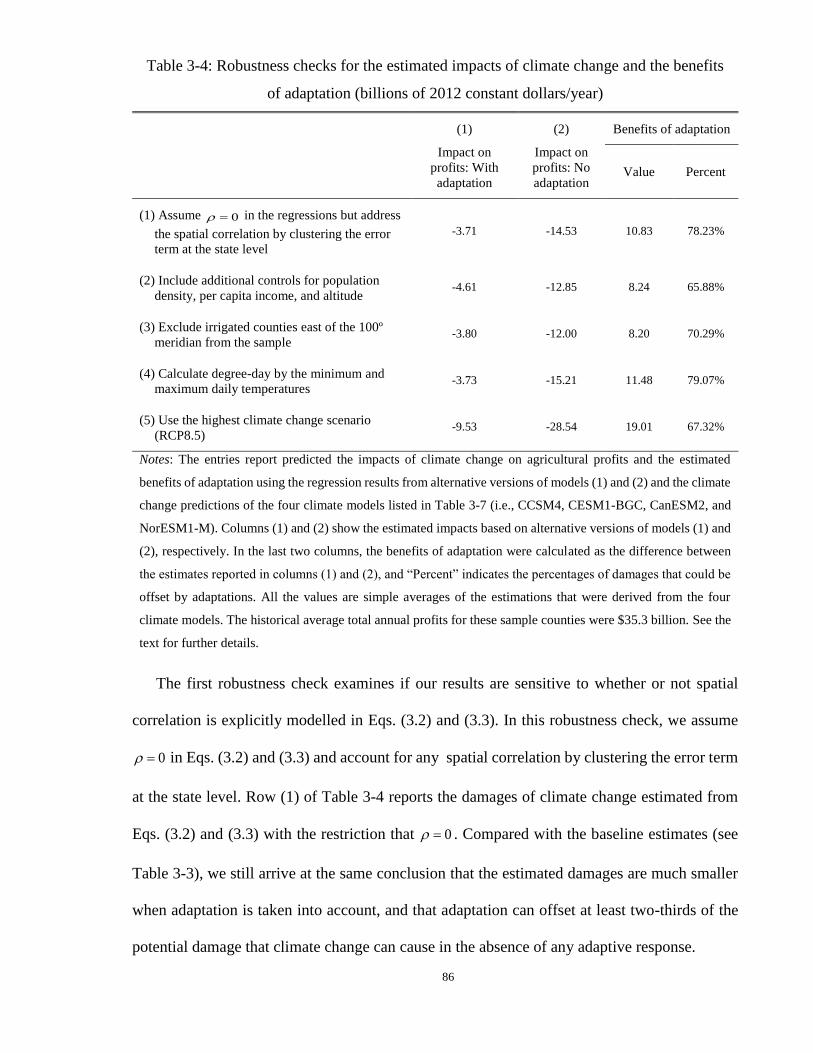
86

Table 3-4: Robustness checks for the estimated impacts of climate change and the benefits

of adaptation (billions of 2012 constant dollars/year)

(1)

Impact on

profits: With

adaptation

(2)

Impact on

profits: No

adaptation

Benefits of adaptation

Value Percent

(1) Assume 0 in the regressions but address

the spatial correlation by clustering the error

term at the state level

-3.71 -14.53 10.83 78.23%

(2) Include additional controls for population

density, per capita income, and altitude -4.61 -12.85 8.24 65.88%

(3) Exclude irrigated counties east of the 100º

meridian from the sample -3.80 -12.00 8.20 70.29%

(4) Calculate degree-day by the minimum and

maximum daily temperatures -3.73 -15.21 11.48 79.07%

(5) Use the highest climate change scenario

(RCP8.5) -9.53 -28.54 19.01 67.32%

Notes: The entries report predicted the impacts of climate change on agricultural profits and the estimated

benefits of adaptation using the regression results from alternative versions of models (1) and (2) and the climate

change predictions of the four climate models listed in Table 3-7 (i.e., CCSM4, CESM1-BGC, CanESM2, and

NorESM1-M). Columns (1) and (2) show the estimated impacts based on alternative versions of models (1) and

(2), respectively. In the last two columns, the benefits of adaptation were calculated as the difference between

the estimates reported in columns (1) and (2), and “Percent” indicates the percentages of damages that could be

offset by adaptations. All the values are simple averages of the estimations that were derived from the four

climate models. The historical average total annual profits for these sample counties were $35.3 billion. See the

text for further details.

The first robustness check examines if our results are sensitive to whether or not spatial

correlation is explicitly modelled in Eqs. (3.2) and (3.3). In this robustness check, we assume

0 in Eqs. (3.2) and (3.3) and account for any spatial correlation by clustering the error term

at the state level. Row (1) of Table 3-4 reports the damages of climate change estimated from

Eqs. (3.2) and (3.3) with the restriction that 0 . Compared with the baseline estimates (see

Table 3-3), we still arrive at the same conclusion that the estimated damages are much smaller

when adaptation is taken into account, and that adaptation can offset at least two-thirds of the

potential damage that climate change can cause in the absence of any adaptive response.

87

In the second robustness check, we examine how sensitive our results are when new control

variables are included. If our results are robust to varying the set of controls, this can be taken

as additional evidence that omitted variable bias, if it exists, is unlikely to be strong enough as

to invalidate our conclusion. Row (2) of Table 3-4 provides the new estimates of Eqs. (3.2) and

(3.3) that now include county-level population density, per capital income, and altitude as

additional controls.30 We find that when these variables are controlled for, the estimated damage

on agricultural profits from the adaptation model is only 4.1 percentage points higher than what

was found without these controls (i.e. the estimated damage rises from 9.0% in the baseline case

to 13.1% here). In addition, based on the new estimates, we find that adaptation could still help

to offset about two-thirds of the damage from climate change. We also tried models that include

only one or two of these three variables and obtain similar results.

The third robustness check explores the consequence of excluding irrigated counties in our

sample. Counties west of the 100º meridian have already been excluded from this study to

address the concern that unmeasurable irrigation differences across regions may give rise to

biased estimates. However, even though the agricultural production of most counties east of the

100º meridian depends on rainfall, some these counties still use irrigation water as a supplement.

30 We do not include these controls in our main regressions because if these variables are not

correlated with climate, omitting them will not cause a bias in the estimation; if they are correlated with

climate, it is most likely that these variables are themselves outcomes of climate but not the cause. In

this case, including these factors in the model will partially eliminate the explanatory power of climatic

variables, even though climate is the true underlying determinant (Dell, Jones, and Olken 2014).

88

In this exercise, we exclude counties east of the 100º meridian that use irrigation.31 As Row (3)

of Table 3-4 shows, whether or not these irrigated counties are excluded does not drive the main

results of this chapter. As such, our results are robust to any unmeasurable irrigation difference

for counties east of the 100º meridian.

The forth robustness check considers another way of calculating degree-day. Following

much of the literature, we have calculated degree-day from the daily mean temperature as the

idea of degree-day was proposed by agronomists who examined the relationship between daily

mean temperatures and the biomass yield of crops via field experiments (Ritchie and NeSmith

1991). Recently, there have been suggestions that degree-day calculated from daily minimum

and maximum temperatures would be a more accurate predictor of crop yields (Schlenker and

Roberts 2009, Tack, Barkley, and Nalley 2015). In this exercise, we follow the method of

(Schlenker and Roberts 2009) to calculate degree-day by minimum and maximum temperatures

and investigate if how degree-day is calculated matters for the results of this study. As shown

in Row (4), when degree-days are calculated by minimum and maximum temperatures, the

damage from climate change predicted by the non-adaptation model (-15.21%) (see Column (2))

remains much larger than the damage predicted by the adaptation model (-3.73%) (see Column

(1)), and the benefit of adaptations in this case (where adaptation can help to offset 79.1% of

the damage without adaptation) is significantly larger than our baseline estimate (72.2%) (see

Table 3-3).

31 We follow Schlenker, Hanemann, and Fisher (2005) to define the counties with more than 20

percent of irrigated farmland as the irrigated counties. We also tried to exclude counties with more than

5 percent or 10 percent of irrigated farmland and obtained reasonably similar results.

89

The fifth and final robustness check re-estimates the impact of climate change under the

highest climate change scenario, namely the RCP8.5 scenario. The RCP4.5 and RCP8.5

scenarios are the medium and upper bound climate change scenarios developed for the latest

IPCC Fifth Assessment Report. So far, we have followed much of the literature in examining

the impact of climate change under the RCP4.5 scenario. In this exercise, we will consider the

climate change projections from the four climate models under the RCP8.5 scenario,32 and for

the adaptation and non-adaptation models, re-estimate the damages of climate change based on

each of these climate projections.

The damage estimates under the RCP8.5 scenario with or without adaptation is reported in

Row (5). Here, we find that both the adaptation and non-adaptation models predict much higher

damages, which is not surprising given the more severe climate change scenario under RCP8.5.

However, just as before, the predicted damages from the adaptation model are much smaller

than what the non-adaptation model predicts, and comparing these predictions shows that

adaptation still has the ability to help offset about two-thirds (67.3%) of the potential damage

from climate change under the RCP8.5 scenario.

32 For example, the predicted mean temperature rise from model CanESM2 under RCP8.5 is 6.3 ºC

by the end of this century, while the predicted mean temperature rise by the same model under RCP4.5

is only 2.3 ºC. When measured in growing season degree-days, the model CanESM2 predicted a 1,199

degree-days rise using RCP8.5 compared to a 583 degree-days rise using RCP4.5.

90

Figure 3-2: Geographic distribution of county-level effects of climate change by the end of

this century under scenario CCSM4 RCP4.5

Notes: the left figure presents the effects that include adaptations and the right figure presents the effects without

adaptations. The county-level effects are calculated by combining the estimated climate coefficients from model

(1) and (2) with the predicted county-level climate changes. Here we take the predictions from climate model

CCSM4 as an example; the geographic distributions of effects predicted from other climate models are quite

similar. The sample includes 2155 rain-fed non-urban counties east of the 100º meridian. All values are expressed

in 2012 constant dollars.

Finally, Figure 3-2 maps the geographic distribution of the climate change impact on

agricultural profits. Taking the climate projection from the CCSM4 climate model as an

example, we calculate the county-level impact with and without adaptations for each county in

our study. From Panel B of Figure 3-2, we can see that warming will hurt the southern counties

will lose but benefit the northern counties. However, if the effect of adaptation is taken into

account, the losses by the southern counties would be smaller while the gains by northern

counties would be larger, as is shown in Panel A. In particular, if predictions are made taking

into account of adaptations, we find that no counties will lose more than 20 dollars per acre per

year (Panel A). However, when adaptations are not taken into account, 863 southern counties

A A B

91

are predicted to lose more than 20 dollars per year and 321 southern counties are predicted to

lose more than 30 dollars (Panel B).

3.5. Concluding remarks

Having a good estimate of what the potential value of adaptation is would be useful from a

policy perspective, especially for informing governments about the benefits of adaptation before

they intervene in helping farmers to adapt. because numerous adaptation measures can

potentially be applied by farmers, it is not feasible to estimate the total benefits of adaptation by

first estimating the benefits accruing to each possible adaptation measure, and then aggregating

these benefits up across all measures. It is also difficult to estimate the benefits of total

adaptations by comparing two models in which one takes adaptation into account and another

reflects the impact of climate change in the absence of any adaptive behavior. This is because

the difference between these two models may also reflect the differences in specification, model

assumptions, and the type of data that they are based upon. To reduce the chance of “comparing

apples and oranges”, this chapter propose an approach that identifies the value of adaptation by

comparing the impact estimates from two panel models, where these models are the same except

for the specification of the fixed effects that these models used.

We find that when taking into account of adaptation, climate change (under the RCP4.5

climate change scenario) could cause the end-of-this-century agricultural profits per year to be

9% less than the current agricultural profits per year, or 3.18 billion dollars less per year in

profits at the end of the century than what we currently observe (at 2012 constant values). If

there are no adaptations, climate change could cause the end-of-this-century agricultural profits

per year to be lower by 30%, or 10.56 billion dollars less per year, instead. Therefore, adaptation

by farmers can help to offset about two-thirds of the potential overall damage from climate

change when adaptation is absent. This conclusion is robust across a number of robustness

92

checks that consider the implications of model specification, omitted variable bias, the influence

of inventory and storage, and alternative climate change scenarios on the impact estimates.

There are several important caveats in explaining the empirical result. First of all, even

though this chapter estimates that there are large potential benefits of agricultural adaptation to

climate change, we do not suggest that the benefits can be exploited by farmers quickly and

freely. This chapter only suggests that if famers can fully adaptation to a climate change, the

benefit of adaptation could be significant. More specifically, we only suggest that, for example,

facing a warming, farmers in a currently cold county of a state could be significantly benefit by

mimicking the production behaviour of farmers currently in a hot county of the same state.

However, adaptation may require significant investments and farmers may not adaptation to a

climate change immediately.

Second, in this partial equilibrium analysis, agricultural prices are assumed constant under

climate change. This assumption is reliable if most of the negative effects in currently hot areas

are offset by the positive effects in currently cold regions. Otherwise, agricultural prices will

rise resulting in a smaller overall profit loss. In this case, the benefits of adaptation tend to be

underestimated. Third, the potential benefits from technological advancements induced by

climate change are not included in the adaptation benefit estimation; hence, this study only

estimates the lower boundary of adaptation benefits. Fourth, to avoid potential bias from

irrigation, we follow the literature and use only data from US counties east of the 100º meridian.

Hence, the results of this chapter apply to only the eastern US and not to the whole country.

Finally, this chapter does not take into account the fertilization effects of higher CO2

concentration. In fact, evidence from agronomic experiments suggest that CO2 concentration

has the potential to offset in part the negative effect of global warming on agriculture, but the

magnitude of this effect is still debated (Long et al. 2006).

93

3.6. Appendix

A. An illustration of the remaining variation after different fixed effects are employed in a

panel model

In Table 3-5, we demonstrate how a generic weather variable would be transformed by

employing certain fixed effects in a climate change impact panel study. To simplify this

discussion, we consider a balanced panel with two years and two counties. In Panel A of Table

3-5, we let itw represent the weather realization of county i in year t , where , 1,2i t . Each

weather observation can be decomposed into three parts: the first part iT represents the county

i’s climate (e.g. the long-term average temperature or precipitation), which has variations across

counties; the second part td measures the inter-annual weather fluctuations that are common

across counties in the same year but vary over time; the last part it represents the county-

specific weather shock. The within-county means and within-year means, which are used in the

discussion below, are also reported in Panel A of Table 3-5.

Panel B of Table 3-5 shows the consequence of including the time fixed effect into a panel

study on climate change, which is to transform the model by subtracting the yearly weather

realizations of each county with the average weather across counties in the same year. Hence,

when the time fixed effect is included, the common inter-annual weather fluctuation ( td ) will

be filtered out by this transformation, and what remains in the weather variation will be

attributed only to the county-specific climate ( iT ) and the county-specific weather shock ( it ).

If the variation pertaining to the latter ( it ) is small, the impact of the weather variable (when

the time fixed effect is included) would then be identified mainly through cross-sectional

climate differences (i.e. 1 2T T or 2 1T T ).

94

Table 3-5: the consequences of fixed effects on the climate change impact panel study

Year 1 Year 2 Within-county mean

A. Panel A. No fixed effects

County 1 11 1 1 11w T d 12 1 2 12w T d 1 2 11 12

12 2

d dT

County 2 21 2 1 21w T d 22 2 2 22w T d 1 2 21 22

22 2

d dT

Within-year

mean 1 2 11 21

12 2

T Td

1 2 12 22

22 2

T Td

B. Panel B. Time fixed effects: subtracting within-year mean from each observation

County 1 1 2 11 21

2 2

T T 1 2 12 22

2 2

T T

County 2 2 1 21 11

2 2

T T 2 1 22 12

2 2

T T

C. Panel C. County fixed effects: subtracting within-county mean from each observation

County 1 1 2 11 12

2 2

d d 2 1 12 11

2 2

d d

County 2 1 2 21 22

2 2

d d 2 1 22 21

2 2

d d

D. Panel D. Two way fixed effects: subtracting within-county and within-year mean, and plus sample mean

County 1 11 12 21 22

4

11 12 21 22

4

County 2 11 12 21 22

4

11 12 21 22

4

Notes: itw is the weather outcome of county i in year t , where , 1,2i t ;

iT represents the climate of

county i , which is assumed to be constant over time but different across counties; td measures the inter-

annual weather fluctuations that are common across counties in the same year but vary over time; it is

the county-specific weather shocks.

Panel C of Table 3-5 shows the consequence of including the county fixed effect into a panel

study on climate change, which is to transform the model by subtracting the within-county mean

from each county. Hence, what remains in the weather variation will be attributed only to the

common inter-annual weather fluctuation ( td ) and the county-specific weather shock ( it ). If

95

the variation pertaining to the latter (it ) is small, the impact of the weather variable would then

be identified mainly through inter-annual weather fluctuation (i.e. 1 2d d or 2 1d d ).

Finally, Panel D of Table 3-5 shows the consequence of including the county fixed effect

along with the year fixed effect. This two-way fixed effect structure eliminates both cross-

sectional differences in the climate ( iT ) and the common inter-annual weather fluctuation ( td ).

As a result, the climate change impact will be estimated mainly by exploiting the variation

pertains to the county-specific weather shock ( it ), which is extremely small as shown in Table

3-1.

B. Data sources and summary statistics

This study makes use of a panel of county-level agricultural production, climate and other

socio-economic and geophysical data for 2155 US counties east of the 100º meridian. This

section provides data sources and summary statistics.

Agricultural production: we follow the literature to construct US county-level agricultural

profits per acre from Census of Agriculture for the census years of 1982, 1987, 1992, 1997,

2002, 2007, and 2012. Agricultural profits are calculated as the difference between agricultural

revenue and agricultural expenditure.33 In this data source, agricultural revenue measures the

before-taxes total market value of all agricultural products sold in a county during a particular

year. These products include livestock, poultry, and other derivative products, as well as crops

that include nursery and greenhouse crops and hay. Agricultural expenditure covers all variable

33 The agricultural profits data is constructed for the years after 1987 since expenditure data are only

available after this time.

96

costs for agricultural production, farm business related interest paid on debts, and maintenance

costs.

As a robustness check, we consider farmland value per acre as another measure of

agricultural productivity.34 Farmland values estimate the value of land and buildings used in

agricultural production. These county-level aggregate measures are divided by farmland area to

obtain the county-level agricultural profits per acre and farmland value per acre, which are the

dependent variables of the econometric study. The farmland area includes acres used in crops,

grazing, and pasture.35

Climate: the daily maximum temperature, minimum temperature and precipitation data from

1981 to 2012 are derived from Parameter-elevation Regressions on Independent Slopes Model

(PRISM 2014). PRISM Climate Group provides 4 × 4 kilometre gridded daily data after the

year of 1981 for the entire US, which is regarded as one of the most reliable small scale climatic

data sets. County-level climate measures are calculated as the simple averages of the climate

cells over the agricultural land within each county. This study follows the literature to construct

the standard county-level measures of climatic variables: growing season degree-days (GDD),

growing season harmful degree-days (GHDD) and growing season total precipitation (GTP)

(Schlenker, Hanemann, and Fisher 2006, Deschênes and Greenstone 2007).

34 The hedonic approach usually considers farmland value per acre as the dependent variable.

Therefore, we follow the same as a robustness check, although we do not focus on it in our paper as it

has little time-variation for a panel study.

35 See previous studies such as Deschênes and Greenstone (2007) for more detailed agricultural

production data descriptions.

97

GDD measures the cumulative exposure to heat between 8 ºC and 32 ºC during the growing

season from April to September. In detail, a day with a mean temperature (say 𝑧̅) below 8ºC

contributes zero degree-days, between 8ºC and 32ºC contributes 𝑧̅ − 8 degree-days, above

32ºC contributes 24 degree-days. GDD is then calculated as the sum of the daily degree-days in

the growing season.

GHDD is calculated as the sum of degree-days above a harmful threshold. We set the

threshold of harmful temperature as 32ºC. Thus, a day with a mean temperature (say 𝑧̅) above

32ºC contributes 𝑧̅ − 32 harmful degree-days; otherwise, it contributes zero harmful degree-

days (Ritchie and NeSmith 1991).36 Finally, GTP is the total precipitation in inches during the

growing season.

Climate predictions: we use the latest high resolution climate predictions from General

Circulation Model (GCM) runs conducted under the Coupled Model Intercomparison Project

Phase 5 (CMIP5) (Taylor, Stouffer, and Meehl 2012). The data of 42 climate projections from

21 CMIP5 GCMs and two Representative Concentration Pathways (RCP) scenarios (RCP4.5

36 The agronomy literature suggests a range of possible thresholds for harmful degree-days. The most

frequently used one is 34 °C (Ritchie and NeSmith 1991). A more recent study that examined nonlinear

temperature effects suggests that crop yields decrease sharply for mean temperatures higher than 29°–

32 °C (Schlenker and Roberts 2009). Since the heat below 32 °C has been included in the calculation of

GDD, we prefer to set the threshold of GHDD as 32 °C. In addition, some studies prefer to calculate

harmful degree-days through daily maximum temperatures. However, most of the heat used to calculate

GHDD in this approach has already been included in the measure of GDD, because a day with a

maximum temperature higher than 34 °C is most likely with the mean temperature below 32 °C.

98

and RCP8.5) 37 are available from the NASA Earth Exchange Global Daily Downscaled

Projections (NEX-GDDP) dataset. 38 Each model provides daily maximum temperature,

minimum temperature and precipitation under various scenarios for the periods from 2006 to

2100, and with a spatial resolution of 0.25 degrees × 0.25 degrees (about 25 km × 25 km). Each

model also provides simulated historical daily data from 1950 to 2005 for the same spatial

resolution. Since point estimates based on a single climate projection can be misleading (Burke

et al. 2015), to estimate the impact of climate change here, we use the climate projection for the

medium scenario RCP4.5 from four of the most widely used CMIP5 models: CCSM4, CESM1-

BGC, CanESM2, and NorESM1-M.39

Control variables: we follow the literature to use a set of county-level soil quality variables

as controls. These data are from the National Resource Inventory and have been widely used.

The soil quality controls include measures of soil salinity, sand content, clay content, K-Factor,

flood risk, permeability, slope length, moisture in top soil, share of wetland and irrigated land.40

37 The RCPs include four climate change scenarios which were developed for the Fifth Assessment

Report of the Intergovernmental Panel on Climate Change (IPCC), and the RCP4.5 and RCP8.5 represent

the medium and highest scenarios, respectively.

38 Data from the NASA Earth Exchange Global Daily Downscaled Projections (NEX-GDDP) dataset

is available from https://cds.nccs.nasa.gov/nex-gddp/.

39 There are over twenty recognized climate change prediction models available, and large prediction

discrepancies are observed across models. We do not have evidence that any particular model is more

reliable than others (Solomon 2007). See http://cmip-pcmdi.llnl.gov/cmip5/availability.html for details

of modelling centres.

40 See Appendix A of Mendelsohn, Nordhaus, and Shaw (1994) for a detailed description of soil

controls.

https://cds.nccs.nasa.gov/nex-gddp/

http://cmip-pcmdi.llnl.gov/cmip5/availability.html

99

Since the land qualities are almost constant over time, the missing values in the soil quality

controls are interpolated. We also use county-level per capita income and population density as

control variables for robustness check.

Irrigation water is heavily subsidized in the US and it is impossible to control for irrigation

differences among counties. In order to avoid the potential bias caused by unmeasurable

irrigation differences, we follow Schlenker, Hanemann, and Fisher (2006) in using only data

from counties east of the 100º meridian, which account for a large proportion (71.6%) of US

agricultural profits. Importantly, in these counties, farming largely relies on rainfall, as opposed

to farming in the arid West that depends mainly on irrigation. As such, we will address the issue

of unmeasurable irrigation differences by focusing on counties east of the 100º meridian.

We also exclude urban counties in this study as farming in these counties usually take place

on a very small scale. Urban counties are defined as counties having a population density of

more than 400 people per square mile (Schlenker, Hanemann, and Fisher 2005). We exclude

counties with missing values during the sample years to form a balanced panel. In doing so, we

are left with 2155 non-urban rain-fed sample counties across the seven census years. All profits

and land prices are translated into 2012 dollars using the GDP implicit price deflator.

100

Table 3-6: A summary of agricultural production data

1982 1987 1992 1997 2002 2007 2012

County average of:

Farmland prices ($1/acre) 2073 1387 1363 1614 1927 2566 3332

Agricultural profits ($1/acre) -- 66 66 83 42 83 99

Areas of land in farms (th. acres) 366 366 362 365 370 372 375

Agricultural expenses ($1/acre) -- 242 253 264 264 335 432

Notes: All entries are county-level averages over the 2155 rain-fed non-urban counties weighted by acres of

farmland. Agricultural profits and expenses are not available prior to 1987. All dollars are in 2012 constant

values.

Table 3-6 summarizes the agricultural production data. Large non-linear variations in

farmland prices and agricultural profits are observed during 1982–2012, but no obvious

correlations can be found between them. The farmland areas remain almost constant, while

agricultural expenses show an increasing trend.

Table 3-7: Summary Statistics of Climate Normal and Climate Predictions

Growing Season:

Average temperature

(°C) GDD (°C) GHDD (°C) GTP (Inches)

Climate Normal

20.23

(3.25)

2272

(558)

0.11

(0.43)

23.50

(3.60)

Predicted climatic changes by the end of this century under scenario RCP45:

CCSM4 1.95

(0.61)

379

(55)

0.38

(0.66)

1.90

(2.17)

CESM1-BGC 2.04

(0.99)

384

(65)

0.49

(1.55)

2.63

(2.97)

CanESM2 2.27

(0.50)

583

(74)

1.47

(3.01)

0.41

(1.61)

NorESM1-M 2.79

(0.80 )

547

(89)

3.13

(4.92 )

1.35

(1.80 )

Notes: All entries are simple averages over the 2155 sample counties. See the text for how the climate

normal and climate predictions are calculated. Standard deviations are reported in parentheses.

101

Table 3-7 reports statistics of climate normal and climate projections (temperature and

precipitation). County-level climate normal is calculated as a 20 year average of the climatic

variable (i.e. average temperature, GDD, GHDD or GTP) from 1981 to 2000 for each county.

The projected county-level climates based on various scenarios for each climate projection

model (i.e. CCSM4, CESM1-BGC, CanESM2 or NorESM1-M) are calculated by the following

steps: Step 1: Map the gridded climate predictions from each climate projection model into each

state to provide state-level climate predictions,41 Step 2: Calculate state-level climate change

predictions as the difference between the predicted 2081–2100 average and the simulated

historical average of 1981–2000 based on each model, Step 3: Add the predicted state-level

climate changes from Step 2 to the county-level climate normal to form county-level climate

predictions for the end of this century.42

Compared with the climate normal, the predicted mean temperature rise based on these four

climate models ranges from 1.95°C to 2.79°C, which is within the range of the best prediction

of mean temperature increase (i.e. 1.0°C to 3.7ºC) by the Intergovernmental Panel on Climate

Change (IPCC) Fifth Assessment Report (2014). Large changes in the GDD are predicted where

41 The spatial resolution of climate predictions does not allow us to calculate the county-level

predictions.

42 The climate normal is usually defined as a 30 year average, but the daily fine scale data before

1981 is not available, and the simulated historical data after 2006 is not provided by CMIP5 models.

Calculating climate normal as a 20 or 30 year average should have no significant effect on climate change

impact predictions. The crucial thing is to make sure that the period during which the climate normal is

calculated is the same as the base period that is used to formulate climate change predictions for each

model, because the model output is not at the same spatial resolution as the observed data (Fisher et al.

2012).

102

the changes range from 379 to 547. The GHDD normal, which is a simple average of GHDD

over all sample counties, is very small (i.e. only 0.11). This comes from the fact that a large

share of counties has a mean temperature of less than 32°C and these countries contribute zero

GHDD.

That being said, 30% of sample counties contribute positive GHDD and 70 hot counties

have more than 1 GHDD (with large standard deviations). Because there are observed counties

with extreme GHDD, we may credibly predict what might happen in the event of hot

temperatures (i.e. when GHDD is large).

Figure 3-3: Geographic distributions of GDD and GTP for climate normal and scenario

CCSM4 RCP4.5

103

Notes: The samples are 2155 rain-fed non-urban counties east of the 100º meridian. This figure compared

the geographic distribution of the climate prediction of the representative scenario CCSM4 RCP4.5 with

the distribution of climate normal.

Lastly, Figure 3-3 compares the geographic distribution of the climatic variables of climate

normal with the distribution of predictions from the representative model CCM4 RCP4.5. The

distributions of predictions from the other three models are quite similar. For the climate normal,

the GDD is decreasing from southern counties to northern counties, and the GTP is decreasing

from east counties to west counties. The predictions from CCSM4 RCP4.5 follow the same

geographic pattern, but predict a hotter and wetter climate. We mapped distributions of the

prediction from other climate models and find similar results.

C. A Bayesian learning simulation of the believed climate trend

This section argues that farmers may not fully recognize and adapt to the recent climate

trends because large inter-annual weather fluctuations accompanied with it may obscure farmers’

recognition of the climate trend. As shown in Figure 3-4, even though there are significant

increasing trend in the yearly mean temperature in the United States from 1960 to 2010, the

inter-annual temperature fluctuation is much larger than the warming trend.

104

Figure 3-4: Yearly mean temperature fluctuations in the US, 1960–2010

Data source: Physical Sciences Division of National Oceanic and Atmospheric Administration

(http://www.esrl.noaa.gov/psd/)

This section provides a simple learning model to show that, even when there are obvious

climate trend, farmers’ perception of the trend is very limited. Assume farmers’ belief of “true”

mean temperature follows a simple Bayesian learning process. Denote farmers’ belief of mean

temperature in period t as tc and with the precision t . In each period, they observe the

realization of temperature ts and update their belief to 1tc using a weighted combination of

prior belief and the realized temperature. Assume the variance ( 2 ) of realized temperature is

unchanged when mean temperature increases, and denote 21/ . According to DeGroot

(1970), for a sudden temperature increase, such as c , in the base year, the farmers’ belief

about mean temperature after T years is given by:

t t tT

t

c T sc

T

105

with 1t t . In expectation, the difference between belied temperature change and true

temperature change is given by:

01 /

cD

T

(3.5)

We combine equation (3.5) with the empirical data as used in Figure 3-4 to draw a

simulation of farmers’ belief. Assume the initial precision of belief ( 0 ) as the inverse of the

variance of temperature during 1960-1970, which is a period before large temperature variance.

Assume the temperature variance during 1970-2010 as 2 . Then we can simulate the evolution

of farmers’ belief after a once for all, for example 5 °C, mean temperature rise in the base year.

The result is shown in Figure 3-5. We find that, after 10 years only about 40 percent of the mean

temperature rise is believed as true temperature rise and only about 80 percent of the change is

believed after 50 years. Since the believed climate change is much small than the actual change,

farmers’ adaptation to recent climate trend is potentially quite limited.

Figure 3-5: A simulation of farmers’ believed “true” temperature rise after an assumed 5 °C

temperature increase in the base year

106

Statement of Authorship for Chapter 4

107

Chapter 4 : The Potential Benefits of Agricultural Adaptation to

Warming in China in the Long Run

Abstract

Abstract: Understanding the extent to which agriculture can adapt to climate change and the

determinants of farmers’ adaptive capacity are of paramount importance from a policy

perspective. Based on a panel of household survey data from a large sample in rural China, the

present chapter adopts a panel approach to estimate the potential benefits of long-run adaptation

and to identify the determinants of farmers’ adaptive capacity. The empirical results suggest

that, for various model settings and climate change scenarios, long-run adaptations should

mitigate one-third to one-half of the damages of warming on crop profits by the end of this

century. These findings support the basic argument of the hedonic approach that omitting long-

run adaptations will dramatically overestimate the potential damage of climate change. The

chapter also finds that household-level capital intensity and farmland size have significant

effects on farmers’ adaptive capacities. (JEL Q15, Q51, Q54)

Keywords: climate change impact, agriculture, adaptation capability

108

4.1. Introduction

Estimating the potential impacts of climate change on agriculture is crucial for understanding

food security issues and for assessing the potential costs associated with the effects of

greenhouse gas emissions (Lobell and Asner 2003). However, any estimate of the impact of

climate change is potentially biased if adaptation measures that are believed to determine the

future severity of the impact of climate change on agriculture are not included (Lobell et al.

2008). Thus, investigating the extent to which effective adaptation measures are likely to be

implemented is central to the study of the potential impact of climate change on agriculture. An

even more interesting issue from a policy perspective is identifying and understanding the

determinants of farmers’ adaptive capacity, as that knowledge can support the design of

effective adaptation policies.

The adaptation of agriculture to climate change is usually defined in terms of production

behavior adjustments by agricultural agents in order to moderate any negative effects or to

exploit beneficial opportunities from the changed climate. Many previous studies have stressed

the difference between long-term adaptations to climate change and short-term responses to

weather fluctuations: in adapting to long-term climate change, farmers can adjust land use and

other ex ante production behaviors, but in responding to random inter-annual weather variations,

farmers can only make limited ex post adjustments due to time constraints or the need for large

fixed investments (Seo 2013). Examining farmers’ responses to inter-annual weather

fluctuations or extreme weather events may shed important light on possible adaptations to

changes in climate variation (see, e.g., Huang, Wang, and Wang 2015). However, in the present

study, we focus only on adaptations to changes in the long-term climate trend; thus, for

simplicity, the term “adaptation” in this chapter refers only to such long-term adaptation to the

climate trend.

109

Empirically, a major contribution to the field of adaptation study involved the hedonic

approach proposed by Mendelsohn, Nordhaus, and Shaw (1994), which implicitly included

adaptations in its climate change impact estimation. The hedonic approach identifies climate

change impacts through cross-sectional climatic differences. Since it is assumed that agricultural

agents will have completely adapted to the climate of their particular regions, by examining how

the local climate in different regions affects the value of farmland, this approach includes a full

range of adaptations. Nevertheless, this approach cannot explicitly evaluate the benefits of

adaptation (Hanemann 2000).

On the other hand, numerous farm-level studies have explicitly estimated the benefits of


the benefits of crop-switching as a method of adaptation, Seo and Mendelsohn (2008) provided

evidence that farmers benefit from switching among different kinds of livestock when adapting

to warming, and Falco and Veronesi (2013) identified the adaptation benefits from adopting

water and soil conservation behaviors. Even though existing farm-level adaptation studies have

dramatically improved our understanding of adaptation, as argued by Mendelsohn, Nordhaus,

and Shaw (1994), in reality, there are innumerable potential adaptation measures that farmers

could apply in response to climate change, and it is impossible to capture the benefits of the full

range of long-run adaptations by examining only individual adaptation measures.

Therefore, an approach to identifying the benefits of long-run adaptations without examining

individual adaptation measures would be valuable. The value of long-run adaptations refers to

the total benefits from all potential adaptation measures that could be taken by farmers given

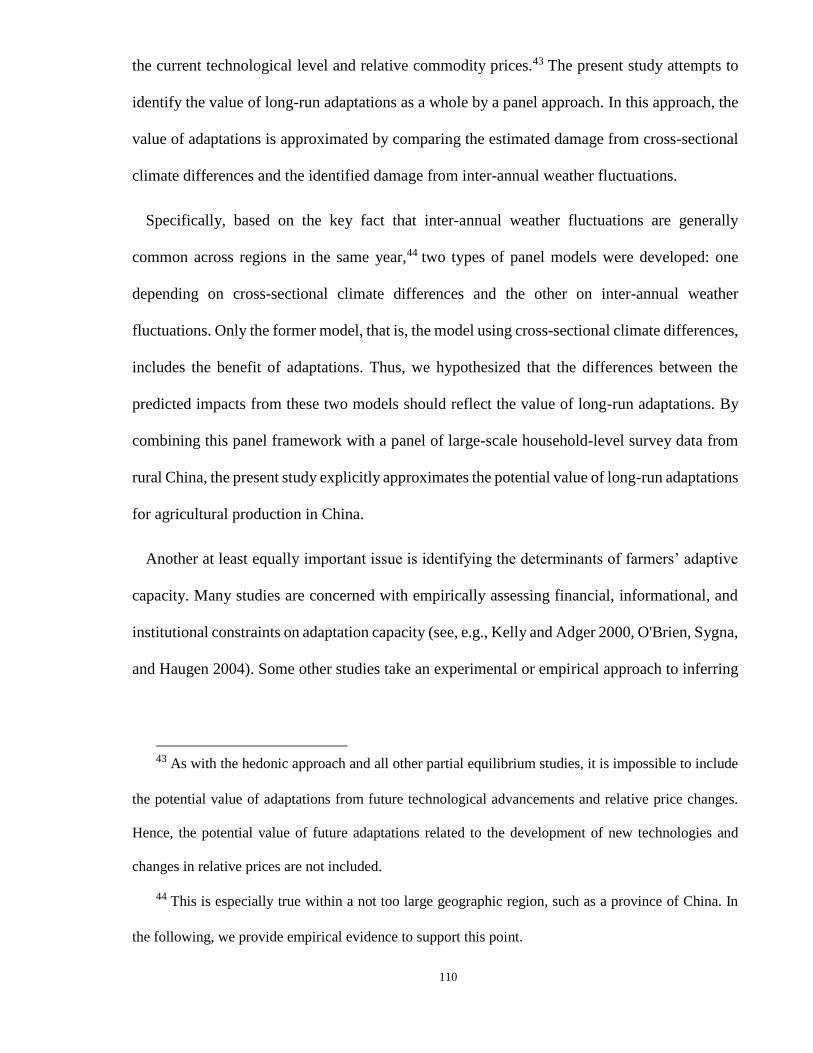
110

the current technological level and relative commodity prices.43 The present study attempts to

identify the value of long-run adaptations as a whole by a panel approach. In this approach, the

value of adaptations is approximated by comparing the estimated damage from cross-sectional

climate differences and the identified damage from inter-annual weather fluctuations.

Specifically, based on the key fact that inter-annual weather fluctuations are generally

common across regions in the same year,44 two types of panel models were developed: one

depending on cross-sectional climate differences and the other on inter-annual weather

fluctuations. Only the former model, that is, the model using cross-sectional climate differences,

includes the benefit of adaptations. Thus, we hypothesized that the differences between the

predicted impacts from these two models should reflect the value of long-run adaptations. By

combining this panel framework with a panel of large-scale household-level survey data from

rural China, the present study explicitly approximates the potential value of long-run adaptations

for agricultural production in China.

Another at least equally important issue is identifying the determinants of farmers’ adaptive

capacity. Many studies are concerned with empirically assessing financial, informational, and

institutional constraints on adaptation capacity (see, e.g., Kelly and Adger 2000, O'Brien, Sygna,

and Haugen 2004). Some other studies take an experimental or empirical approach to inferring

43 As with the hedonic approach and all other partial equilibrium studies, it is impossible to include

the potential value of adaptations from future technological advancements and relative price changes.

Hence, the potential value of future adaptations related to the development of new technologies and

changes in relative prices are not included.

44 This is especially true within a not too large geographic region, such as a province of China. In

the following, we provide empirical evidence to support this point.

111

the determinants of adaptive capacity under climate change by examining farmers’ responses to

extreme weather conditions or natural disasters (see, e.g., Grothmann and Patt 2005, Huang,

Wang, and Wang 2015). These studies shed important light on the determinants of adaptive

capacity and generally imply that farmers with better infrastructure, higher crop diversification,

more financial and technical support, and better information are better at adaptation.

However, since previous studies lack an explicit estimate of the overall value of long-run

adaptations, they generally evaluate the determinants of a specific adaptation behavior but not

the determinants of overall adaptive capacity. Our study’s panel approach allows us to explicitly

identify the potential value of long-run adaptations as a whole, so it is possible to examine the

factors influencing overall adaptive capacity. In our data set, complete farm and household

characteristics are included. By combining these farm and household characteristics with the

value of long-run adaptations, we were able to examine the influence of these characteristics on

adaptation value and gain additional understanding of the determinants of farmers’ adaptive

capacity.

Three characteristics distinguish this chapter from previous studies. First, this chapter

investigates the benefits of long-run adaptations of agriculture to climate change in China, while

most previous studies examined the damage from climate change (see, e.g., Wang et al. 2009,

Chen, Chen, and Xu 2016). Second, in this study, the value of a full range of long-run

adaptations can be explicitly estimated, whereas the hedonic studies only implicitly include the

potential benefits of a range of long-run adaptations and other studies only explicitly examine

the benefits of one or a few specific adaptation measures. Third, this chapter provides empirical

evidence on the determinants of the value of long-run adaptations in China.

The following sections describe the study’s data sources and summary statistics, conceptual

framework and econometric models, and empirical results.

112

4.2. Data sources and summary statistics

The data for agricultural production and household characteristics were collected from a large-

scale household-level survey conducted in rural China in late 2012 and early 2013. Funding was

available for the field survey in eight of the 34 provinces and regions of China (see Figure 4-1).

The survey was dependent on funding from several separate projects supporting research in

specific provinces or regions, so it was conducted only in those provinces supported by these

projects. Specifically, the survey in the provinces of Hebei, Henan, Anhui, Shandong, and

Jiangsu was mainly supported by funding from Ministry of Science and Technology in China,

the survey in the provinces of Jiangxi and Yunnan was mainly supported by funding from the

Australian Centre for International Agricultural Research, and the survey in Jilin province was

mainly supported by National Natural Sciences Foundation in China.

Even though which provinces were included in the survey depended on funding availability,

the eight sample provinces approximately represent the various agricultural systems in China.

Specifically, the Jilin province represents the monoculture agricultural system in cold areas of

China; Hebei, Henan, Anhui, Shandong, and Jiangsu represent the rotation agricultural system

in China’s temperate climate zone; the Jiangxi province represents rice production in southern

China; and the Yunnan province represents agricultural production in the plateau climate zone.

Thirty-one sample counties were selected from the eight sample provinces. We selected three

sample counties from each of seven sample provinces, but we selected 10 sample counties from

Jiangxi because extra funding was available for this province. Within each sample province, we

divided all the counties into three groups (10 groups for Jiangxi) based on the condition of the

agricultural production infrastructure and randomly selected one county from each group.

113

Figure 4-1: Sample provinces of the survey in China.

We selected the townships and villages before interviewing the actual households. Within

each of the 31 selected counties, we divided all the townships into three groups based on the

condition of the agricultural production infrastructure and randomly selected one township from

each group. We used the same approach to select three villages from each township. Finally, we

randomly selected 10 households for face-to-face interviews in each sampled village. We

identified a total of 2,790 households in the eight provinces. After dropping the households with

missing data for agricultural output, input, or household characteristics, the final sample used in

the analysis comprised 2733 households.

114

The farmlands in the survey are mainly used for crops and orchards.45 The crop production

and orchard data were collected separately. For land used for crop production, only the larger

two plots were investigated if the household managed more than two plots. This sample

selection rule helped to reduce measurement error because, in our data set, each household

managed 7.6 plots on average and some plots were quite small. Collecting data from small plots

might incur large measurement errors because, according to our experience, it is harder for

farmers to precisely recall unit land inputs and outputs for a small plot. There is no major

concern about the representativeness of the sample plots selected because, on average, the larger

two plots took up 86.3 percent of the cropland area managed by each farmer. For orchards, the

data were collected for all orchards managed because each household usually managed only one

or two orchards.

Household-level agricultural profits per hectare were collected for two years from 2010 to

2012.46 According to the survey, farmers usually plant multiple crops in sequence in a plot

45 Forestry and animal husbandry were excluded from this survey because, in our sample provinces,

mainly local governments, not households, manage the forests. In addition, the household-level animal

husbandry in the sample is mainly free ranging and usually does not take up farmland. Orchards comprise

fruits, vegetables, and nut-producing trees.

46 This is because another purpose of this survey was to investigate the effects of natural disasters

(drought and flood) on agricultural production. For each county, the year with the highest loss and the

year with the lowest loss due to natural disasters were selected out of the three years from 2010 to 2012.

Thus, the two sample years may differ between some counties, and consequently we can form only an

unbalanced panel from this data set. To avoid the potential bias introduced by this sample selection rule,

we include the percentage of profit loss due to natural disasters as a control variable in the following

econometric regressions.

115

within a year. The main growing season is usually used for staple crops, such as rice, wheat,

and maize, while other seasons are used for minor crops, such as oilseed rape, beans, and

vegetables. The profits per hectare were constructed as revenue minus cost. The revenues were

the market value of all the products harvested in a year, and the costs were the total production

expenditure in a year. The costs included only expenses for seed, fertilizers, pesticides, labor,

and machinery.47 Finally, the profits per hectare were translated into US dollars (USD) using

China’s rural Consumer Price Indices (CPI) and the exchange rate between RMB and USD as

of 2010. In the following econometric analyses, we mainly used crop profits per hectare as the

dependent variable. As a robustness check, we also provide analyses using the weighted average

of profits per hectare from cropland and orchards as the dependent variable.

46 Since the family members of each household provide most of the labor input, the labor costs are

measured as the total labor inputs (in work days) for each hectare of farmland times the daily wage. The

daily wage is the average daily wage for agricultural labor in each village.

116

Table 4-1: Definition of variables

Variables Definition

Dependent variable

Crop profits Profits from crop production only (2010 constant USD/ha)

Crop and orchard profits Average profits from cropland and orchards weighted by land area

(2010 constant USD/ha)

Climate variables

Degree-day Yearly degree-day (degrees)

Degree-day2 Square of yearly degree-day

Precipitation Yearly total precipitation (mm)

Precipitation2 Square of yearly total precipitation

Farm and household characteristics

Capital intensity Production capital per hectare (1000 USD/ha)

Land size Land area managed by a household (ha)

Labor intensity Labor input per hectare (days/ha) †

Education Education of head of household (years)

Age Age of head of household (years)

Other control variables

Irrigation Irrigation water used per year per hectare (m3/ha)

Disaster loss Loss per hectare caused by natural disasters (%)

Market access Distance to the nearest market of production inputs (km)

Soil quality County-level land quality measured by loam in the soil (%)#

Road density County-level density of paved road and railway (km/km2)§

†: The labor intensity is measured by the total working days per hectare per year. Since there are usually multiple

growing seasons within a year, the labor inputs are the sum across growing seasons within a year.

#: Loam is a standard indicator of soil quality. Loam is considered ideal for agricultural uses because it retains

nutrients well and retains water, while still allowing excess water to drain away. The data come from Resources

and Environment Data Centre of Chinese Academy of Sciences (http://www.resdc.cn/).

§: The road density is calculated by the authors from a shapefile of 1:100,000 scale road information map for the

year 2008 in China. Road density is measured as the kilometers of paved road and railway within a county divided

by the total area of the county.

Detailed farm and household characteristics with the potential to affect agricultural profits

and adaptive capacity were also collected in the survey. As defined in Table 4-1, these

117

characteristics include the capital intensity, labor intensity, and farmland size of the household;

education level and age of the head of household; irrigation water used per hectare; agricultural

loss per hectare caused by natural disasters; and market access. County-level agricultural land

quality and road density were also included as control variables. County-level land quality was

measured as the percentage of loam in the soil, while county-level road density was measured

as the number of kilometers of paved road and railway within a county divided by the total area

of the county. The summary statistics of the data are provided in Table 4-2.

Table 4-2: Summary statistics of variables

Variables Mean Standard

deviation

Minimum

value

Maximum

value

Crop profits (USD/ha) 2186 1465 -2048 22156

Crop and orchard profits (USD/ha) 2259 1638 -2048 34922

Degree-day (degrees/year) 3472 999 1941 5688

Precipitation (mm/year) 1182 707 302 2866

Capital intensity (1000 USD/ha) 59.1 77.3 1.0 898.4

Land size (ha) 2.2 5.5 0.0 44.5

Labor intensity (days/ha) 0.5 0.8 0.0 19.0

Education (years) 6.8 3.0 0.0 16.0

Age (years) 52.8 10.3 18.0 88.0

Irrigation (m3 /ha) 2788 3287 0.0 14991

Disaster loss (%) 10.6 10.8 0.0 100.0

Market access (km) 2.2 3.1 0.0 25.0

Loam (%) 30.9 4.9 21.8 40.0

Road density (km/km2) 0.5 0.3 0.2 1.1

Note: The definitions of the variables are provided in Table 4-1.

The county-level daily mean temperature and precipitation data were derived from the China

Meteorological Data Sharing Service System (http://cdc.nmic.cn). This data set provides real

data for each of the 677 meteorological stations throughout China and offers the most detailed

118

and reliable climate data set in China. At least one meteorological station is sited in 22 of the 31

sample counties. For those counties with more than one meteorological station, county-level

climate was calculated as the sample average from all the meteorological stations within the

county. For the nine sample counties in which meteorological stations were not available, we

instead used climate data from the nearest meteorological station.48

Daily mean temperature and precipitation were used to construct values for county-level

yearly degree-days (DD) and yearly total precipitation (TP). 49 DD measures cumulative

exposure to temperatures of between 8°C and 32°C during the year. For example, a day with a

mean temperature below 8°C contributes zero DDs, between 8°C and 32°C it contributes the

difference between the mean and 8°C, and above 32°C it contributes 24 DDs. DD is the sum of

daily measures across the calendar year. TP is the total precipitation in mm during the calendar

year. For the robustness test in the econometric analysis, we also calculated the growing season

48 The alternative meteorological stations used were within a distance of 20km from the nearest

border of the sample county.

49 Some previous studies focusing on only one or several crops used growing season heat and

precipitation measures. In the present study, since the agricultural profits relate to all crops planted in

the plots during the whole year and not to only a specific crop, and since crops have quite different

growing seasons, we preferred to use the yearly measures instead of the growing season measures.

According to the survey, multiple planting in sequent seasons is a common practice in middle and low

latitudes of China, and in some provinces plants are usually growing in every season of the year. For

example, farmers in Yunnan province usually plant potatoes in the same plots after harvesting rice each

September, while farmers in Jiangxi province plant oilseed rape from January to April before the

temperature is high enough for other crops. Hence, it is impossible to find a discrete “growing season”

in the present study.

119

degree-day and growing season total precipitation. We followed the literature in defining

growing season to be from March to October.

Finally, to predict climate change impacts, we collected the latest climate change projections

that were developed for the Fifth Assessment Report of the Intergovernmental Panel on Climate

Change (IPCC). The climate projections from 21 modeling centers and two Representative

Concentration Pathway (RCP) scenarios, namely RCP4.5 and RCP8.5, which represent the

medium and highest scenarios, respectively, were downloaded from the NASA Earth Exchange

Global Daily Downscaled Projections (NEX-GDDP) data set (https://cds.nccs.nasa.gov/nex-

gddp). Each model provides daily minimum temperature, maximum temperature, and

precipitation under each scenario for the periods from 2006 to 2100, with a spatial resolution of

0.25 degrees × 0.25 degrees (about 25 km × 25 km). Each model also provides simulated

historical daily data from 1950 to 2005 for the same spatial resolution.

Table 4-3: Predicted changes in yearly climatic variables

Climate change

scenario Variable Mean

Standard

deviation

Minimum

value

Maximum

value

RCP4.5

Mean temperature 2.7 0.3 2.4 3.3

Degree-day 684.0 127.2 500.2 941.0

Total precipitation (mm) 98.2 76.2 12.1 240.5

RCP8.5

Mean temperature 5.2 0.5 4.6 6.2

Degree-day 1400.7 211.4 1056.4 1668.0

Total precipitation (mm) 109.7 66.5 21.9 215.5

Note: The predicted changes in climatic variables are calculated as the differences between the 30-

year historical average (1976–2005) and the 30-year prediction average (2071–2100).

The climate change predictions were calculated as the difference between the 1976–2005

average and the 2071–2100 average. Specifically, we first mapped the gridded climate

predictions into each sample province to formulate province-level climate predictions for each

year, then calculated the 30-year historical simulation average (1976–2005) and the 30-year



120

prediction average (2071–2100) for each province.50 Since point estimates depending on a

single climate projection can be misleading (Burke et al. 2015),51 we used the average prediction

of the CMIP5 models in the following impact estimation. Table 4-3 reports the projected climate

changes of scenarios RCP4.5 and RCP8.5. The projected yearly mean temperature rise is 2.7ºC

and 5.2ºC for RCP4.5 and RCP8.5, respectively. Despite the dramatic difference in the change

of yearly degree-day predicted by these two scenarios, their predicted precipitation changes are

quite similar.

4.3. Conceptual framework and econometric approach

Two sources of meteorological variation are usually employed to identify the impact of climate

change: cross-sectional climate differences used in the hedonic approach, such as in

Mendelsohn, Nordhaus, and Shaw (1994), and inter-annual random weather fluctuations

adopted by panel studies, such as in Deschênes and Greenstone (2007).52 Econometric methods

based on these two sources of meteorological variation differ in their ability to incorporate long-

run adaptations. Specifically, climate change impacts identified through cross-sectional climate

50 The spatial resolution of climate predictions does not allow us to calculate the county-level

predictions.

51 There are over twenty recognized climate change prediction models available, and large prediction

discrepancies are observed across models. We do not have evidence that any particular model is more

reliable than the others (Solomon 2007). For details of the modeling centers, see “CMIP5 Coupled Model

Intercomparison Project,” Program for Climate Model Diagnosis and Intercomparison, http://cmip-

pcmdi.llnl.gov/cmip5/availability.html.

52 “Climate” describes the long-term average of weather outcomes for a given region, while “weather”

refers to a particular year’s realization of climate distribution (Dell, Jones, and Olken 2014).



121

variations should include the benefit of long-run adaptations because, as assumed in the hedonic

approach, farmers should have adapted to the climate of their regions (Mendelsohn, Nordhaus,

and Shaw 1994). On the other hand, impacts identified through inter-annual weather fluctuations

do not include the benefits of long-run adaptations since farmers will have made only limited

ex post adjustments in response to random weather outcomes (Seo 2013).

Even though the hedonic approach provides a potentially ideal way to implicitly incorporate

long-run adaptations into climate change impact studies, this approach cannot be used to

estimate explicitly the value of adaptations (Hanemann 2000). Therefore, the merits of the

hedonic approach depend crucially on the magnitude of the value of long-run adaptation: if the

value of long-run adaptions is negligible, using the method depending on inter-annual weather

fluctuations will not result in a significant bias due to omitting adaptations. In addition,

explicitly estimating the value of long-run adaptations is necessary for identifying the

determinants of overall adaptive capacity. Hence, an econometric approach that can be used to

estimate the value of long-run adaptations is valuable.

Based on the key fact that inter-annual weather fluctuations are generally common across

regions in the same year, Huang (2015) combined the basic idea of the hedonic approach with

panel data and developed a panel framework that could be used to estimate explicitly the value

of long-run adaptations. The basic idea of this panel framework is shown as equation (4.1):

it i t itw T d (4.1)

in which itw is the weather outcome of county i in year t ;

iT is the climate (i.e., long-term

average weather outcome) of county i , which is assumed to be constant over time but differ

across counties; td measures the inter-annual weather fluctuations that are common across

counties in the same year but vary over time; and it represents county-specific weather

122

shocks.53 In a panel model with time fixed effects, the inter-annual weather fluctuations that are

common across observations (td ) can be filtered out, and thus the remaining meteorological

variation pertains only to cross-sectional climate differences (iT ) and idiosyncratic local shocks

(it ). Since the local shocks are quite small (as shown in Table 4-4), the impacts are mainly

identified through cross-sectional climate differences, and therefore the long-run adaptations

are included. On the other hand, the county fixed effect can be used to eliminate inter-county

differences in climate 𝑇𝑖, which is constant over time, with the remaining variation pertaining

only to common inter-annual weather fluctuations (td ) and county-specific weather shocks

(it ). Since the variation in county-specific weather shocks is very small, the impacts are mainly

identified through the common inter-annual weather fluctuations and thus do not include

adaptation benefits.

53 Here, we assume the climate of a county

iT is constant for not too long time (such as three years).

However, relaxing this assumption does not affect the weather decomposition as shown in equation (1).

Because the climate trend over time is usually common across counties (as shown in Table 4), it can be

captured in the second parttd .

123

Table 4-4: The magnitudes of inter-county climate variation and local weather shocks

C. Panel A. Percentage of counties with temperature variance below/above (°C):

±0.1 ±0.2 ±0.3 ±0.4

Inter-county mean temperature variation 96.7 93.5 90.3 74.2

County-specific temperature shocks 22.5 4.3 2.1 0.0

D. Panel B. Percentage of counties with precipitation variance below/above (mm):

±100 ±200 ±300 ±400

Inter-county total precipitation variation 96.7 93.5 83.9 64.5

County-specific precipitation shocks 18.3 5.4 4.3 2.1

Note: Temperature is measured by the yearly mean temperature (°C), while the precipitation is

measured by the yearly total precipitation (mm). The “inter-county mean temperature variation” and

the “inter-county total precipitation variation” represent the climate (i

T ) differences, which are

calculated as the deviation of the county mean from the sample mean. The “county-specific

temperature shocks” and the “county-specific precipitation shocks” measure the variation in local

shocks (it ), which are calculated as the remaining variation after the county mean and the year

mean are subtracted from each observation. All entries are calculated for the sample counties and

sample years (2010–2012). See the text for further details.

Table 4-4 shows the actual size of the variation pertaining toit and

iT . We found that 74.2

percent of the sample counties had deviations in their yearly mean temperature (iT ) from the

sample mean that were larger than 0.4°C, while no counties had county-specific temperature

shocks (it ) higher than 0.4°C (see Panel A of Table 4-4). The same result applied to

precipitation, with 64.5 percent of the counties having more than 400 mm of deviation from the

yearly total precipitation (iT ) from the sample mean and only 2.1 percent of counties having

local precipitation shocks (it ) of more than 400 mm (see Panel B of Table 4-4). These results

support our argument that climate change impacts can be identified mainly through inter-county

mean climate differences in a panel model with time fixed effects and through common inter-

annual weather fluctuations in a panel model with county fixed effects.

124

However, since these climatic variables were calculated only for a three-year panel, it is likely

that the small county-specific temperature and precipitation shocks, as shown in Table 4-4, are

the result of too short a panel period. To test this possibility, we calculated the values for the

same variables as shown in Table 4-4 using 30 years of weather data for the sample counties

and found quite similar results. Since the magnitudes of inter-annual weather fluctuations were

quite similar across regions, it is reasonable to find small county-specific weather shocks after

removing the inter-county climate differences and the common inter-annual weather

fluctuations. Similar results have been found in previous studies using US data (Fisher et al.

2012).

The panel model used to identify climate change impact through cross-sectional climate

differences is shown in equation (4.2), in which ijty denotes the crop profits per hectare of

household i in county j and year t; itC is a vector of county-level climate variables, including

yearly DD, yearly total precipitation, and their quadratic terms; ijtL is a vector of the farm and

household characteristics as shown in Table 4-1, including capital intensity, land size, labor

intensity, head of household education and age, irrigation, disaster loss, and market access; jtK

is a vector of the county-level soil quality and transportation controls as defined in the last two

rows of Table 4-1; , , and are coefficients; and pt represents the province-by-year

dummy. The dummy was used to filter out year-to-year weather and other fluctuations that were

common across counties within each province.54 Thus, the coefficients of the climate variables

54 The province-by-year fixed effect equates to imposing an individual-year fixed effect for each

province. Since China covers a large geographic area, the province-by-year fixed effect is better than the

individual-year fixed effect in accounting for inter-annual common fluctuations.

125

in this model were identified mainly through the inter-county mean climate differences, and the

benefits of adaptations could then be included. Finally, in the estimation, the error term 𝜇𝑖𝑡 is

clustered at the province level in order to address the potential bias from the spatial correlation

of the error term (Deschênes and Greenstone 2007, Fisher et al. 2012).

' ' '

ijt jt ijt jt pt ijty C L K (4.2)

The model used to identify climate change impacts through inter-annual weather fluctuations

is presented in equation (4.3). The settings for ijty , jtC , ijtL , and jtK are the same as for equation

(4.2). The only difference is in the use of fixed effects. Model (4.3) includes the county fixed

effects j to eliminate inter-county climate differences and does not use any type of time fixed

effects, as these tend to eliminate most of the year-to-year weather fluctuations.55 Thus, the

climatic coefficients are mainly identified through the year-to-year weather fluctuations and do

not include the benefits of adaptations. Finally, the error term ijt is clustered at the province

level.

' ' '

ijt jt ijt jt j ijty C L K (4.3)

By combining the estimates of the climate variables from models (4.2) and (4.3) with the

climate change predictions, we were able to project the impacts with and without adaptations,

55 In equation (3) we are not seeking to control for the effect of price shocks induced by output

fluctuations because the price shock can be seen as farmers’ “natural insurance” for weather fluctuations.

Eliminating price shocks would thus overestimate the impact of weather fluctuations (Fisher et al. 2012).

126

respectively. The differences in the projected impacts between these two models can be

interpreted as the benefits of long-run adaptation.

The most significant advantage of this approach is evaluating the value of long-run

adaptations as a whole, thus freeing the analyst from the burden of estimating the value of each

of the innumerable adaptive responses by farmers. This advantage is derived directly from the

basic idea of the hedonic approach: obtaining information about adaptations to future climate

change by examining the current production differences across climate regions.56 Large cross-

sectional climate differences are observed, and farmers should have adapted to the long-run

climate of their regions.

A large body of studies has shown that climate has tremendous effects on agricultural

production across regions, and most of the cross-sectional differences in agricultural production

practices resulting from climatic differences can be explained as the result of farmers’ long-run

adaptation to the climate of their regions. Specifically, the distributions of crop types and crop

varieties across regions are mainly the result of farmers’ adaptive choices based on their long-

run climate observations. Regional gradients of temperature result in the distribution of different

crops and varieties from north to south (Cramer and Solomon 1993, Ramankutty et al. 2002),

56 Another way of forecasting adaptations to future climate change is by examining farmers’

responses to historical climate change. Unfortunately, the historical climate changes were too small for

the period during which agricultural production data is available. For example, the Inter-government

Panel on Climate Change report of 1995 indicated that mean surface air temperature increased by about

0.3~0.6 °C in the prior 100 years, while the best prediction of mean temperature increase by the end of

this century is about 2.5 °C (see scenario RCP4.5 of Table 3). Hence, the available historical time-series

data may not offer much information about farmers’ potential adaptations to future climate change.

127

while for regions with sufficiently warm temperatures, cultivation is strongly determined by the

distribution of precipitation (Leemans and Solomon 1993).

Even though crop choice is critically dependent on climate, humans have adopted various

other adaptive behaviors to overcome natural limitations to some extent. In response to the

observed climate, farmers in different climate regions choose the optimal farm-management

practices for their regions. For example, the sowing time in the temperate zones of northern

China is much later than it is in the tropics of southern China so that crops have sufficiently

warm temperatures during germination (Chen, Hu, and Yu 2005); moreover, busting is usually

chosen in southeast China where precipitation is abundant during the growing season, while

conservation tillage measures are taken by farmers in northwest China where precipitation is

quite limited (Zhang et al. 2011). In modern agricultural production, additional adaptive

measures are available that depend on intensive investments, such as the adoption of greenhouse

and ground water irrigation systems to address insufficiency in growing season temperature and

precipitation (Jin and Young 2001, Thomas 2008).

Even though climate differences and farmers’ adaptive behaviors can explain many cross-

sectional production differences, many other non-climatic factors also have significant effects.

For example, differences in land quality, transportation, and the availability of ground water for

irrigation also have significant effects on variations in agricultural profits. Nevertheless, cross-

sectional climate differences can still be a useful instrumental variable for identifying the

benefits of adaptation to future climate change. As suggested by Dell, Jones, and Olken (2014),

non-climatic variables with the potential to influence agricultural profits and also correlate with

climatic variables are themselves most likely the result of climate but not the cause of it.

Omitting these variables will not necessarily result in biased estimates of the coefficients of

climatic variables. Moreover, in our econometric analyses, we did our best to control for non-

128

climatic determinants of agricultural profits, including capital intensity, land size, labor intensity,

head of household education and age, irrigation, disaster loss, market access, land quality, and

transportation.

4.4. Empirical results

The regression results are shown in Table 4-5. Columns 1a and 1b present the regression results

from model (4.2) and model (4.3), respectively, using crop profits as the dependent variable,

while columns 2a and 2b represent the regression results from model (4.2) and model (4.3),

respectively, using the average profits of crops and orchards as the dependent variable.57 For all

of the four regressions, the estimated coefficients of the yearly degree-day are statistically

significant and show the inverted U-shaped relationship that is usually found in climate change

impact studies and indicates agricultural profits increasing with degree-day up to a turning point,

after which they decline.

The coefficients of precipitation are all statistically insignificant, presumably because the

control variables, especially the household-level detailed control for irrigation, and the fixed

effects account for a significant share of the effects of precipitation. Previous studies have

generally found that precipitation is not a good measure of water supply for crops grown,

especially for irrigated agriculture (Schlenker, Hanemann, and Fisher 2005). In the data, the

agricultural production of 78.0 percent of households depends on irrigation, so control for

irrigation is necessary. Even though we included a detailed measure of current irrigation water

used, we don’t have a good measure of the future availability of irrigation water. Hence, the

57 The magnitudes of the estimated coefficients of model (4.2) and model (4.3) are not directly

comparable because different fixed effects are used. However, as shown in the following, the impacts

calculated from these coefficients are comparable.

129

estimated effects of the predicted changes in precipitation are unreliable. Therefore, in the

following calculation of the impacts of climate change and the benefits of adaptations, we

mainly focus on the effects of warming.

Most of the control variables in these four regressions have statistically significant effects on

profits per hectare. Specifically, profits per hectare increase with increasing capital intensity

until a turning point, after which the effect becomes negative, but the negative effect is

negligible (the coefficient of the square term is approximate to zero). The effect of land size on

profits also shows an inverted U-shaped relationship. In addition, profits per hectare rise

significantly with the education level of the head of household and the volume of irrigation

water used, and decline significantly with losses due to natural disasters and the distance to

market. All these significant effects are quite intuitive.

130

Table 4-5: Regression results of the effects of climatic variables and household characteristics

on agricultural profits

Independent variables Crop profits Crop and orchard profits

(1a) (1b) (2a) (2b)

Climate variables

Degree-day (100 degrees/year) 200.99* 1,148.51*** 183.21* 1,040.01***

(107.10) (188.95) (87.25) (221.23)

Degree-day2 -3.20* -15.29*** -3.03* -13.48***

(1.62) (2.91) (1.33) (3.41)

Precipitation (100 mm/year) 76.04 -45.27 84.27 -39.00

(70.09) (39.82) (70.67) (46.62)

Precipitation2 -2.44 2.66 -2.51 2.59

(2.44) (1.36) (2.43) (1.60)

Farm and household characteristics

Capital intensity (1000 USD/ha) 14.60* 21.00** 19.97* 24.56**

(6.28) (9.05) (8.67) (10.60)

Capital intensity2 -0.00*** -0.00** -0.00** -0.00*

(0.00) (0.00) (0.00) (0.00)

Land size (ha) 357.71** 344.45*** 429.03** 445.74***

(120.44) (49.53) (148.81) (58.00)

Land size2 -20.76* -20.60*** -23.63* -25.52***

(9.75) (3.91) (11.73) (4.57)

Labor intensity (days/ha) 2.41 1.33** 1.78 0.75

(1.40) (0.61) (1.31) (0.72)

Labor intensity2 -0.00 0.00 -0.00 0.00

(0.00) (0.00) (0.00) (0.00)

Education (year) 15.27* 15.89*** 21.41** 21.30***

(7.51) (6.11) (8.41) (7.15)

Age (year) 1.03 -0.22 -0.68 -2.61

(2.59) (1.90) (2.15) (2.23)

Other controls

Irrigation (m3/ha) 0.04** 0.02*** 0.05** 0.03***

(0.02) (0.01) (0.02) (0.01)

Disaster loss (%) -37.23*** -36.50*** -36.74*** -36.05***

(4.94) (1.66) (4.11) (1.95)

Market access -44.51** -27.18*** -41.72** -26.00***

(16.19) (6.86) (15.59) (8.03)

Soil quality control 27.85 - 32.27 -

(21.92) (22.44)

Road density control 336.06 - 478.85 -

(255.36) (285.75)

Province-by-year fixed effects Yes No Yes No

County fixed effects No Yes No Yes

Observations 5,466 5,466 5,466 5,466

R-squared 0.213 0.248 0.166 0.198

Note: The definitions of the variables are given in Table 4-1. Stand errors clustered at the province-

level are reported in parentheses. Coefficients of soil quality control and road density control are omitted

in columns 1b and 2b because these county-level variables are mainly time invariant and have been

accounted for by the county fixed effects. Significance levels are *** p <0.01, ** p <0.05, * p <0.1.

131

We combined the estimated coefficients of degree-day and degree-day square of models (4.2)

and (4.3) with the climate change scenarios to predict the impacts of warming with and without

long-run adaptations, respectively. Row (1) of Table 4-6 reports the predicted yearly impact of

warming on crop profits per hectare by the end of this century for two scenarios. The model that

did not include long-run adaptations predicted much more damage (column 2) than the model

that included long-run adaptations (column 1) for both scenarios. The t-test as reported in

column (3) found statistically significant differences between the estimated impacts with and

without long-run adaptations.

Specifically, under the median climate change scenario RCP4.5, the predicted changes in crop

profits per hectare will be -163.7 USD and -370.6 USD with and without long-run adaptations,

respectively. These damages correspond to 7.5 percent and 17.0 percent of the current mean

annual profits per hectare in the sample area (see Table 4-2). Column (4) reports the percentage

of damages that will be offset by long-run adaptations. Long-run adaptations will help to

mitigate 55.8 percent and 56.1 percent of the damages predicted by the model that did not

include long-run adaptations for scenarios RCP4.5 and RCP8.5, respectively. In addition,

relatively large standard deviations from the estimated damages were found, implying that there

are significant regional differences in the impacts of warming.

132

Table 4-6: Impacts of warming on crop profits by the end of this century and the benefits of

long-run adaptation (2010 constant USD per hectare per year)

Model setting Scenario

Impacts (3)

T-value of

the t-test

between

columns

(1) and (2)

(4)

Percentage

of damages

offset by

adaptation

(%)

(1)

With

adaptation

(2)

No

adaptation

(1) Impacts of

warming on crop

profits

RCP4.5 -163.7 -370.6 26.5*** 55.8

(92.7) (397.5)

RCP8.5 -908.0 -2069.7 58.2*** 56.1

(223.9) (1019.4)

Robustness tests

(2) Including the

effects of changes

in precipitation

RCP4.5 -154.6 -313.1 17.6*** 50.6

(119.9) (454.1)

RCP8.5 -842.8 -1981.1 57.6*** 57.5

(307.6) (986.4) (3) Excluding

household

characteristics and

soil controls in the

regressions

RCP4.5 -217.9 -375.5 20.1*** 42.0

(114.3) (394.1)

RCP8.5 -1208.9 -2095.1 43.1*** 42.3

(328.2) (1022.3)

(4) Using the profits

from both crops and

orchards as the

dependent variable

RCP4.5 -169.9 -268.8 12.3*** 36.8

(104.2) (408.6)

RCP8.5 -977.8 -1654.2 44.4*** 40.9

(184.5) (774.6)

(5) Using growing

season climatic

variables

RCP4.5 -144.0 -221.5 8.8*** 35.0

(72.0) (454.1)

RCP8.5 -1041.5 -1559.9 222.8*** 33.2

(82.9) (88.2) Note: Standard deviations are reported in parentheses. Significance levels are *** p <0.01, ** p

<0.05, * p <0.1. See the text for further details.

Row (2) to row (5) of Table 4-6 provide robustness tests. The main analysis as shown in row

(1) only includes the effects of warming. In row (2), the effects of changes in precipitation are

also included in the estimation. We find that including precipitation in the estimation does not

significantly change the estimated impacts and adaptations. Both models estimated slightly

smaller damages for each scenario, and adaptations are still expected to offset about half of the

damages.

133

A potential concern of panel model (2), which depends on inter-county climate differences,

is omitted-variable biases. Even though the inter-annual common fluctuations and the inter-

province time-invariant differences are well controlled by the province-by-year fixed effects,

we did not control for within-province inter-county differences apart from the controls listed in

Table 4-1. To test for potential omitted-variable bias, we dropped all household-level controls

and the soil-quality control from the regression. As shown in row (3), the estimated benefits of

long-run adaptation drop from 55.8 percent to 42.0 percent for scenario RCP4.5 and from 56.1

percent to 42.3 percent for scenario RCP8.5. The results are similar if we only exclude control

subgroups. Since omitting all these crucial determinants of crop profits only reduces the

adaptation benefits by about 12 percent, the remaining omitted variables might not cause a large

bias.

The main analysis only includes profits from annual crops. Because the responses of perennial

plants to climate change might be different from those of annual crops, including the profits

from orchards for which production is mainly dependent on perennial plants, the analysis might

lead to a different adaption estimate. Row (4) of Table 4-6 shows this possibility. The impacts

are estimated from regressions that used the weighted average of profits from crops and orchards

as the dependent variable. For the model with long-run adaptations, the estimated impacts are

quite similar to the impacts on crop profits. However, the model without long-run adaptations

predicted significantly smaller damage than that reported in row (1), presumably because

perennial orchards are more resistant than annual crops to inter-annual weather fluctuations. As

reported in the last column, long-run adaptations will still help to reduce a significant share of

the damages (i.e., 36.8 percent under scenario RCP4.5 and 40.9 percent under scenario RCP8.5).

Since adjusting the growing season may be an important way of adapting to climate change,

in the main analysis, we use yearly climatic variables instead of growing season climatic

134

variables to allow for the adjustment of growing seasons in the long run. Intuitively, using

growing season climatic variables in the estimation will underestimate the benefits of adaptation.

In row (5), we provide the estimates using growing season climatic variables with a fixed

growing season from March to October. As expected, the estimated benefits of adaptation drop

to 35.0 percent for scenario RCP4.5 and to 33.2 percent for RCP8.5. The main conclusion

remains that omitting long-run adaptations will dramatically overestimate the damages.

Finally, we investigated the effects of farm and household characteristics on the benefits of

adaptation. We first calculated the impacts of warming predicted by RCP4.5 on crop profits for

each household using the estimates from column (1a) and (1b) of Table 4-5, respectively.

Second, we calculated the household-level adaptation value as the difference in the impact

estimated from these two models. Third, we performed a regression analysis of the household-

level values of adaptation against the farm and household characteristics listed in Table 4-1 and

controlled for the mean temperature differences among counties. The significant regression

coefficients are reported in equation (4.4)58:

*** 7*** 2***

*** *** 2 ** **

*** *** 2

Adaptation_value 10.4 Capital_intensity 2.3 Capital_intensity

65.5 Land_scale 6.1 Land_scale 7.3 Age 0.01 irrigation

4.4 Degree-day 0.001 Degree-day

e

(4.4)

We found that the cross-sectional adaptation value first decreased and then increased with the

degree-day. In other words, very cold and very hot areas have higher adaptation values than

temperate areas. This result is intuitive, because farmers in cold areas have more potential to

58 We also tried the regressions using adaptation values calculated from other warming scenarios

and found almost no differences in the significance levels and effect directions of each variable.

135

adopt adaptation measures to exploit the beneficial opportunities of warming, while farmers in

hot areas are more likely to take adaptation measures to moderate the negative effects of

warming.

More importantly, both capital intensity and farmland size have statistically significant effects

on the adaptation value. For farmers with limited production capital, increases in capital

intensity will raise their adaptive capacity. When production capital is quite abundant, further

increases in capital intensity will reduce the value of adaptation, presumably due to decreasing

returns from physical capital investment, but the negative effects are negligible (the coefficient

of the square term is only 72.3e ). Hence, a government policy targeted at enhancing farmers’

adaptive capacity can work by encouraging investment in the physical capital of agricultural

production.

On the other hand, the value of adaptation decreases with farmland size at first and then

increases after a turning point. A possible explanation is that, for small household farms in China,

increasing farmland size means less labor can be input per hectare of land in response to

warming. However, once the land size is large enough, modern agricultural production methods

such as mechanized agriculture production are available to reduce labor force constraints. Hence,

for those areas with the possibility of significantly increasing their household-level farmland

size, a government policy to increase farmland size would enhance adaptive capacity.

In addition, the age of the head of household also had a statistically significant negative effect

on adaptation value. This could reflect the fact that old farmers have less adaptation ability than

young farmers. Finally, agricultural production that depends more heavily on irrigation had

lower adaptation values. This could be explained by the fact that irrigation is itself an adaptation,

so currently irrigated farms might experience lower marginal benefits than currently non-

irrigated farms from further irrigation improvements.

136

4.5. Conclusions

This chapter provides empirical support for the basic argument of the hedonic approach that

omitting long-run adaptations will dramatically overestimate the damage of climate change.

Depending on large-scale household-level survey data from rural China, the empirical results

show that long-run adaptations are able to offset one-third to one-half of the damages of

warming using various model settings and climate change scenarios. Hence, omitting long-run

adaptations will dramatically overestimate the damages of warming. This study also finds that

capital intensities and farmland size have significant effects on farmers’ adaptive capacities.

There are several important caveats to the empirical results. First, the potential benefits from

future technological advancements induced by climate change are not included in the estimation.

Hence, this study estimates only the lower boundary of adaptation benefits. Second, forestry

and animal husbandry were excluded from the survey. If it is possible for farmers to adapt to

warming by switching land use among crops, animal husbandry, and forestry, this study would

tend to underestimate the benefits of long-run adaptation. Third, in this partial equilibrium

analysis, agricultural prices are assumed to be constant during climate change. This assumption

is reliable if the positive effects in currently cold regions offset most of the negative effects in

currently hot areas. Otherwise, agricultural prices will rise and the benefits of adaptation will be

even greater.

137

Chapter 5 : Concluding Remarks

Having a good understanding of the relationship between climate change and agricultural

production can help policy makers to better anticipate issues concerning food security. However,

although there is a growing econometric literature on this topic, there is also much disagreement

on what exactly the effect of warming is: Whether it is positive or negative, or if there is an

effect at all. Using a standard meta-analysis, Chapter 2 of the thesis identifies some potential

sources of this disagreement using the estimates of the effect of warming on agricultural output

from 130 primary studies.

The role of adaptation is central to the debate surrounding the impacts of climate change on

agriculture. Understanding how much adaptation is likely to occur is central to any study of the

impact of climate change and is also of paramount importance from the policy perspective.

Chapter 3 of the thesis combines the basic idea of the traditional hedonic approach with the

panel method proposed by Deschênes and Greenstone (2007), developing a panel framework

that can be used to incorporate a full range of adaptations to climate change and to explicitly

estimate the value of adaptation.

An even more interesting issue from the policy perspective is to identify and understand the

determinants of farmers’ adaptation capability, as that knowledge can support the design of

effective adaptation policies. Using large-scale household-level survey data from rural China,

Chapter 4 of the thesis employed the panel framework developed in Chapter 3 to identify the

determinants of adaptation capability.

138

5.1. Souces of the heterogeneity in the climate change impact literature

Chapter 2 conducts a meta-analysis based on 130 primary econometric studies to better

understand the conflict among the existing estimates of warming on agriculture. We carried out

a broad and inclusive search of the rapidly growing econometric based literature that examines

the effect of climate change on agricultural output. In all, we selected 130 papers based on

several criteria.

The summary statistics of the primary studies suggest that (1) differences in model

specification of the primary studies may account for different conclusions; (2) differences in

certain study characteristics (e.g. the latitude of the region in which the study is based on) may

also explain why the econometric estimates disagree; (3) the conflicting results could be due to

publication bias, which refers to the fact that research with ‘statistically significant’ results tend

to be published more often than those with ‘negative’ results. According to these summary

statistics, 10 characteristics of primary studies were chosen as the independent variables in the

meta-regression.

The meta-regressions find that 10 independent variables explain a significant proportion of

the variation in the primary estimates. For example, the adjusted R2 of 64.89% indicates that the

10 independent variables account for 64.89% of the variation in the primary estimates. Most of

the independent variables are statistically significant. The location of the primary studies can

influence the estimates of the effect of warming on crop yield. For instance, the coefficient of

latitude is positive and statistically significant, which implies that studies based on higher

latitude regions are more likely to report positive effects of warming than studies based on lower

latitude regions.

Publication bias and biological differences in crops are also important in accounting for the

disagreement among primary studies. Under the Publication Bias category, the coefficient on

139

research time is positive and statistically significant, which implies that studies that are

published more recently tend to report positive effects more frequently than those published

earlier. The coefficient of publication status is negative and statistically significant, which

means published papers or books are more likely than unpublished materials to report negative

effects. Under the Biological Differences category, the significant coefficients on the dummies

for maize, soybean, and rice but not wheat imply that the effects of warming can differ for

different crops.

The specification of the econometric model has a strong influence on the eventual estimated

effects of warming as well. Under the Model Specification category, the variables measures of

output, temperature measures, and data types are all positive and statistically significant. To

investigate the relative importance of model specification in explaining the disparity among the

primary studies, we conducted a regression analysis for each sub-category of variables.

Comparing the adjusted R2 across the four sub-category regressions, we find that model

specification has the strongest influence on the primary estimates. In particular, differences in

model specification can explain 30% of the disagreement among primary studies, whereas 15%

of the disagreement can be explained by biological differences in crops, 12.4% by regional

differences, and 9.8% by publication bias.

Given that differences in model specification account for the largest share of the

disagreement, we investigate the extent to which these studies could be reconciled if they had

adopted a certain set of specifications. We find that if the primary studies use the yearly

temperature measure and adopt the hedonic modelling approach, their estimates will have less

dispersion and will tend to concur with the prediction from the simulation-based literature that

warming will lead to positive effects on agriculture in the high latitudes but damages in the low

latitudes.

140

5.2. The extent to which US agriculture will adapt to climate change

Understanding how much adaptation is likely to occur is central to any study of the impact of

climate change on agriculture and is also of paramount importance from the policy perspective.

However, an effective approach for evaluating the benefits of potential adaptations has not yet

been developed. Chapter 3 of the thesis develops a panel framework to estimating the potential

value of adaptation.

This panel framework depends on the basic idea that impacts identified through cross-

sectional climate differences should include the benefit of a full range of adaptations because,

as assumed in the hedonic approach, farmers should have adapted to the climate of their regions.

On the other hand, impacts identified through inter-annual weather fluctuations will not include

the adaptations to long-run climate change since farmers have only limited ex-post adjustments

in response to random year-to-year weather fluctuations, and this short-run response is not seen

as adaptation to climate change. Two types of panel model were developed to estimate the

potential impacts of climate change. One depended on cross-sectional climate differences and

the other on inter-annual weather fluctuations. Only the former model, that is, the model using

cross-sectional climate differences, included the benefit of adaptations. Hence, the differences

between the predicted impacts from these two models should reflect the value of a full range of

adaptations.

To estimate the climate change impacts on US agriculture and the potential values of

adaptation, this study combines this panel framework with a panel of county-level agricultural

production, climate, and other socio-economic and geophysical data for 2155 US counties east

of the 100º meridian. We follow the literature to construct US county-level agricultural profits

141

and farmland value per acre from the Census of Agriculture for the census years of 1982, 1987,

1992, 1997, 2002, 2007, and 2012. The daily maximum temperature, minimum temperature,

and precipitation data from 1981 to 2012 are derived from the Parameter-elevation Regressions

on Independent Slopes Model (PRISM). We also use the latest high-resolution climate

predictions from general circulation model (GCM) runs conducted under the Coupled Model

Intercomparison Project Phase 5 (CMIP5).

The econometric estimations conclude that, for estimates from the model that includes

adaptations, the overall impacts on agricultural profits are negative but generally quite small.

The changes in agricultural profits from climate predictions per year and by the end of this

century are, in billions of 2012 constant USD, -1.27 (-3.6%, CCSM4), -1.57 (-4.4%, CESM1-

BGC), -4.63 (-12.3%, CanESM2) and -5.52 (-15.6%, NorESM1-M). On the other hand, the

model that does not include adaptations predicts relatively large falls in agricultural profits,

ranging from USD -5.96 (-16.8%) to -16.14 (-45.7%) billion for different climate predictions.

The average impacts of these four climate predictions are 9% with adaptations and 30% without

adaptations.

We calculate the benefit of adaptation as the difference between estimates of the models

with and without adaptations. The benefit of adaptation ranges from USD 4.69 to 10.62 billion

per year, and this benefit increases with the level of predicted warming. Adaptations will help

to offset 78.7%, 78.2%, 66.3% and 65.8% of potential output loss from the predicted climate

change given by CCSM4, CESM1-BGC, CanESM2 and NorESM1-M, respectively. On average,

adaptation is estimated to reduce 72.4% of the overall predicted damages from climate change.

Hence, omitting adaptation from models will dramatically overestimate the impacts.

142

The main conclusions of this study are quite robust to numerous specification checks.

Specifically, under the medium climate change scenario, RCP4.5, the predicted changes in

climate will lead to mild damages if adaptations are included. In addition, potential adaptations

will help to offset at least two-thirds of the damages predicted by the model that does not include

adaptations, even under the highest climate change scenario, RCP8.5.

5.3. Determinants of farmers’ adaptation capability in rural China

Understanding the determinants of farmers’ adaptation capability is of paramount importance

from a policy perspective, especially for developing countries where agricultural production is

potentially most vulnerable to climate change. However, most of the adaptation study involved

the hedonic approach proposed by Mendelsohn, Nordhaus, and Shaw (1994), which implicitly

includes adaptations in its climate change impact estimation. The benefits of adaptations cannot

be explicitly evaluated by this approach. In addition, most of the farm-level studies explain the

responses to weather fluctuations as adaptations, so interpretation of these studies might have

precluded some of the potential benefits of long-term adaptation from adjusting ex ante

production behaviors.

Therefore, an approach to identifying the benefits of a full range of adaptations without

examining individual adaptation measures would be valuable. The value of examining the full

range of adaptations as a whole refers to the total benefits from all potential adaptation measures

that could be taken by farmers given the current technological level and relative commodity

prices. However, this is not yet possible, as an effective approach to evaluating the benefits of

a full range of adaptations has not been developed. The present study attempts to identify the

value of a full range of adaptations using the panel approach proposed in Chapter 3.

143

In this approach, the value of adaptations was approximated by comparing the damages

estimated from cross-sectional climate differences and the damages identified from inter-annual

weather fluctuations. Specifically, based on the key fact that inter-annual weather fluctuations

are generally common across regions in the same year, two types of panel model were developed:

one depended on cross-sectional climate differences, and the other on inter-annual weather

fluctuations. Only the former model, that using cross-sectional climate differences, included the

benefit of adaptations. Thus, we hypothesized that the differences between the predicted impacts

from these two models should reflect the value of a full range of long-term adaptations.

By combining this panel framework with a panel of large-scale household-level survey data

from rural China, the present study not only predicts the potential damage of global warming

on agricultural profits with farmers’ adaptations applied, but also explicitly approximates the

potential value of a full range of long-term adaptations. We find that agricultural profits increase

with climate variables up to a turning point, after which they decline. In addition, most of the

farm and household characteristics have statistically significant effects on agricultural profits.

For example, labor intensity has a negative and statistically significant effect on agricultural

profits. A potential explanation for this is that because labor is abundant in rural China, higher

labor input will drive down the marginal labor output. The effect of capital intensity is positive

and statistically significant, which implies that increased capital input per hectare will enhance

agricultural profits per hectare. This reflects the fact that production capital is scarce in rural

China. Finally, agricultural profits increase significantly with the volume of irrigation water

used and decrease with losses caused by natural disasters.

We combined the estimated coefficients from the econometric models with the climate

change scenarios to predict the impacts of warming with and without adaptations, respectively.

We found that the model that did not include adaptations predicted twice as much damage as

144

the model that included adaptations for both scenarios. If we include adaptations, by the end of

this century, the predicted changes in agricultural profits per year, per hectare, will be

USD -196.9 billion (scenario RCP4.5) and USD -996.3 billion (scenario RCP8.5), which

corresponds to 8.4% and 42.5% of the current mean annual profits per hectare in China,

respectively. In addition, relatively large standard deviations for the estimated damages are

found, implying that there are significant regional differences in the impacts of warming.

As expected, the model without long-term adaptations consistently predicted much higher

impacts than the model with adaptations, and furthermore, the value of adaptation increased

almost linearly with warming. The values of adaptations ranged from USD 225.8 billion to USD

1512.8 billion per hectare per year (in 2010 constant dollars). Interestingly, we found that, for

various degrees of warming, long-term adaptations will always help to offset about 50% of the

damages predicted by the model that does not include long-term adaptations.

More importantly, the regression coefficients of farm and household characteristics implied

that labor intensity and capital intensity have a statistically significant positive effect on the

adaptation value. Farmers with higher labor and capital intensity will be good at adaptation.

However, the farmers’ education level had a negative effect on adaptation value. A possible

explanation is that educated people have higher opportunity costs of adaptation. In addition, the

age of the household head also had a statistically significant negative effect on the adaptation

value; this may reflect the fact that old farmers have less adaptation ability than young farmers.

Finally, agricultural production that depends more heavily on irrigation had lower adaptation

values.

145

5.4. Policy recommendations

Food security is at increasing pressure owing to diminishing returns from technological

advances and world population growth; yet, changes in climate may make the situation even

worse. To address this threat, policy makers need to be informed by robust empirical evidence

on the effect that global warming has on agricultural production. Understanding how much

adaptation is likely to occur is central to any study of the impact of climate change on agriculture

and is also of paramount importance from the policy perspective. The role of adaptation is

central to the debate surrounding the impacts of climate change on agriculture. Even more

interesting from a policy perspective are the determinants of adaptation capability, because

identifying the determinants of farmers’ adaptation capabilities can support the design of

effective adaptation policies.

To illustrate the importance of including adaptations in the climate change impact study,

this thesis develops a panel framework that can be used both to incorporate a full range of

adaptations to climate change and to explicitly estimate the value of adaptation. Combining this

framework with empirical data from the United States and China we find that, if the potential

adaptations are taken into account, the overall impact of climate change on the agricultural

production of these two countries is quite small. The overall fall in US agricultural profits will

be about 9% per year by the end of this century, and the potential impact of climate change on

agricultural profits in China will be about 8.4% annually.

If adaptations are omitted or farmers cannot adapt to the climate change, however, the

overall damage will be much higher: 30% of profits in the United States and 18% in China.

Therefore, improving farmers’ adaptation capabilities will be crucial in reducing the damage

caused by climate change from a policy perspective. The empirical study in Chapter 4 found

that increasing farm-level labor and capital intensities will significantly enhance farmers’

146

adaptation capabilities, presumably because adaptation requires a large amount of labor and

capital input. Hence, a government policy providing incentives for farmers to invest more time

in managing their farms will lead to a higher adaptation level and less damage due to climate

change. In addition, a government policy with the target of improving the capital intensity of

agricultural production will also enhance farmers’ adaptation capabilities and reduce the overall

damage from climate change.

5.5. Limitation and further studies

In Chapter 2 of the thesis, a standard meta-analysis is applied to identify some potential sources

of the disagreement among econometric studies concerning the climate change impacts on

agriculture. However, because studies summarized in the meta-analysis usually utilize different

units, we can only use the z-value of the marginal effect of warming at the mean as the meta-

dependent variable. Even though using the z-value as the meta-dependent variable helps to make

primary studies comparable, much useful information is omitted. For example, if we can use the

coefficients of climate variables as the meta-dependent variable, the global-level overall impacts

of climate change can be identified by the meta-analysis. Efforts to adjust the units of primary

studies and to make the coefficients from primary studies comparable will lead to a more

sophisticated meta-analysis that can provide further policy recommendations.

The panel method proposed in Chapter 3 provides a potential method for identifying the

value of adaptations under climate change. Even though this method has the advantage of

identifying adaptations, it is potentially vulnerable to omitted variables. Although the inter-

annual fluctuations that are common across counties and the time-invariant differences among

states are well controlled by the fixed effects, we do not control for inter-county differences

within each state. In order to account for the inter-county unobservable differences, county-

fixed effects are applied in previous studies. The cost of applying county-fixed effects is

147

eliminating all inter-county climate differences. As a result, no signals can be used to

incorporate adaptations. We conducted numerous tests to ensure the omitted variables would

not cause significant biases in our estimation; however, further studies developing an approach

that avoids the omitted variables biases would be valuable.

Another potential bias of our study in Chapter 3 comes from the measurement error of

agricultural profits data. A potential concern of using annual agricultural profits as the

dependent variable is the potential bias results from yearly storage and inventory adjustments.

The annual profits data from the US Census of Agriculture measures the difference between

reported sales and expenditures during the same year. However, in response to output and price

changes caused by weather fluctuation, farmers tend to adjust their storage and inventory in

order to maximize total discounted profits. As a result, some of the outputs of this year might

be sold in the next year, or part of this year’s profits might come from last year’s production. In

further studies, developing a way to adjust the bias derived from the agricultural profits data

will help to provide more precise estimates of climate change impacts and the value of

adaptations.

In addition, there are several important caveats in explaining the empirical result of

Chapter 3. First, this study does not take into account the fertilization effects of higher CO2

concentration. In fact, evidence from agronomic experiments suggests that CO2 concentration

has the potential to offset in part the negative effect of global warming on agriculture, but the

magnitude of this effect is still debated. Second, in this partial equilibrium analysis, agricultural

prices are assumed to be constant under climate change. This assumption is reliable if most of

the negative effects in currently hot areas are offset by the positive effects in currently cold

regions. Otherwise, agricultural prices will rise, resulting in a smaller overall profit loss. Third,

to avoid potential bias from irrigation, we follow the literature and use only data from US

148

counties east of the 100º meridian. Hence, the results of this chapter apply only to eastern US

and not to the whole country. Fifth, the potential benefits from technological advancements

induced by climate change are not included in the adaptation benefit estimation. Previous studies

show that technological advancements may play an important role in agricultural adaptation to

climate change (Emerick et al. 2016). Consequently, this study estimates only the lower

boundary of adaptation benefits.

Finally, the conclusions of Chapter 4 depend heavily on the sample areas. Based on a panel

of household survey data from rural China, Chapter 4 adopts the panel approach developed in

Chapter 3 to estimate the potential benefits of adaptation and to identify the determinants of

farmers’ adaptation capability. In the survey, only 31 counties in eight sample provinces were

selected to represent the various agricultural systems in China. However, provinces and counties

in China different dramatically in conditions of agricultural production, such as the irrigation

water availability, soil quality, and transportation costs. Further studies that expand the sample

areas should lead to more reliable conclusions.

149

References

Adams, Richard M. 1989. "Global climate change and agriculture: an economic perspective."

American Journal of Agricultural Economics 71 (5):1272-1279.

Adams, Richard M, Cynthia Rosenzweig, Robert M Peart, Joe T Ritchie, Bruce A McCarl, J

David Glyer, R Bruce Curry, James W Jones, Kenneth J Boote, and L Hartwell Allen.

1990. "Global climate change and US agriculture." Nature 345:219-224.

Anselin, L. 1988. Spatial Econometrics: Methods and Models. Vol. 4: Springer Science &

Business Media.

Becker, Betsy Jane, and Meng-Jia Wu. 2007. "The synthesis of regression slopes in meta-

analysis." Statistical Science:414-429.

Bel, Germà, Xavier Fageda, and Mildred E Warner. 2010. "Is private production of public

services cheaper than public production? A meta‐regression analysis of solid waste

and water services." Journal of Policy Analysis and Management 29 (3):553-577.

Belotti, Federico, Gordon Hughes, and Andrea Piano Mortari. 2014. "XSMLE: Stata module

for spatial panel data models estimation." Statistical Software Components.

Burke, Ingrid C, CM Yonker, WJ Parton, CV Cole, DS Schimel, and K Flach. 1989. "Texture,

climate, and cultivation effects on soil organic matter content in US grassland soils."

Soil science society of America journal 53 (3):800-805.

Burke, Marshall, John Dykema, David B Lobell, Edward Miguel, and Shanker Satyanath. 2015.

"Incorporating climate uncertainty into estimates of climate change impacts." Review

of Economics and Statistics 97 (2):461-471.

Burke, Marshall, and Kyle Emerick. 2015. "Adaptation to Climate Change: Evidence from US

Agriculture." Working paper, University of California, Berkeley.

150

Burke, Marshall, and Kyle Emerick. 2016. "Adaptation to Climate Change: Evidence from US

Agriculture." American Economic Journal: Economic Policy 8 (3):106-140.

Card, David, and Alan B Krueger. 1995. "Time-series minimum-wage studies: a meta-analysis."

The American Economic Review:238-243.

Cavlovic, Therese A, Kenneth H Baker, Robert P Berrens, and Kishore Gawande. 2000. "A

meta-analysis of environmental Kuznets curve studies." Agricultural and Resource

Economics Review 29 (1):32-42.

Challinor, AJ, J Watson, DB Lobell, SM Howden, DR Smith, and N Chhetri. 2014. "A meta-

analysis of crop yield under climate change and adaptation." Nature Climate Change 4

(4):287-291.

Chen, Shuai, Xiaoguang Chen, and Jintao Xu. 2016. "Impacts of climate change on agriculture:

Evidence from China." Journal of Environmental Economics and Management 76:105-

124.

Chen, Xiaoqiu, Bing Hu, and Rong Yu. 2005. "Spatial and temporal variation of phenological

growing season and climate change impacts in temperate eastern China." Global

Change Biology 11 (7):1118-1130.

Conway, Gordon, and Gary Toenniessen. 1999. "Feeding the world in the twenty-first century."

Nature 402:C55-C58.

Cramer, Wolfgang P., and Allen M. Solomon. 1993. "Climatic classification and future global

redistribution of agricultural land." Climate Research 3 (1-2):97-110.

De Hoyos, Rafael E, and Vasilis Sarafidis. 2006. "Testing for cross-sectional dependence in

panel-data models." Stata Journal 6 (4):482.

DeGroot, Morris H. 1970. Optimal Statistical Decisions. New York: McGraw-Hill.

151

Dell, Melissa, Benjamin F. Jones, and Benjamin A. Olken. 2012. "Temperature Shocks and

Economic Growth: Evidence from the Last Half Century." American Economic Journal:

Macroeconomics 4 (3):66-95. doi: doi: 10.1257/mac.4.3.66.

Dell, Melissa, Benjamin F. Jones, and Benjamin A. Olken. 2014. "What Do We Learn from the

Weather? The New Climate-Economy Literature." Journal of Economic Literature 52

(3):740-98.

Deschênes, Olivier, and Michael Greenstone. 2007. "The Economic Impacts of Climate Change:

Evidence from Agricultural Output and Random Fluctuations in Weather." The

American Economic Review:354-385.

Di Falco, Salvatore. 2014. "Adaptation to climate change in Sub-Saharan agriculture: assessing

the evidence and rethinking the drivers." European Review of Agricultural Economics

41 (3):405-430.

Di Falco, Salvatore, Marcella Veronesi, and Mahmud Yesuf. 2011. "Does adaptation to climate

change provide food security? A micro-perspective from Ethiopia." American Journal

of Agricultural Economics 93 (3):829-846.

Disdier, Anne-Célia, and Keith Head. 2008. "The puzzling persistence of the distance effect on

bilateral trade." The Review of Economics and statistics 90 (1):37-48.

Elhorst, J. Paul. 2010. "Spatial Panel Data Models." In Handbook of Applied Spatial Analysis,

edited by Manfred M. Fischer and Arthur Getis, 377-407. Springer Berlin Heidelberg.

Emerick, Kyle, Alain de Janvry, Elisabeth Sadoulet, and Manzoor H Dar. 2016. "Technological

innovations, downside risk, and the modernization of agriculture." American Economic

Review 106 (6):1537-61.

Falco, Salvatore Di, and Marcella Veronesi. 2013. "How Can African Agriculture Adapt to

Climate Change? A Counterfactual Analysis from Ethiopia." Land Economics 89 (4).

152

Fisher, Anthony C, W Michael Hanemann, Michael J Roberts, and Wolfram Schlenker. 2012.

"The Economic Impacts of Climate Change: Evidence from Agricultural Output and

Random Fluctuations in Weather: Comment." The American Economic Review 102

(7):3749-60.

Frees, Edward W. 2004. Longitudinal and panel data: analysis and applications in the social

sciences: Cambridge University Press.

Gechert, Sebastian. 2015. "What fiscal policy is most effective? A meta-regression analysis."

Oxford Economic Papers:gpv027.

Golnaraghi, Maryam, and Rajiv Kaul. 1995. "The science of policymaking: Responding to

ENSO." Environment: Science and Policy for Sustainable Development 37 (1):16-44.

Grothmann, Torsten, and Anthony Patt. 2005. "Adaptive capacity and human cognition: the

process of individual adaptation to climate change." Global Environmental Change 15

(3):199-213.

Hanemann, W Michael. 2000. "Adaptation and its measurement." Climatic Change 45 (3):571-

581.

Huang, Jikun, Yangjie Wang, and Jinxia Wang. 2015. "Farmers' Adaptation to Extreme Weather

Events through Farm Management and Its Impacts on the Mean and Risk of Rice Yield

in China." American Journal of Agricultural Economics 97 (2):602-617.

Iršová, Zuzana, and Tomáš Havránek. 2013. "Determinants of horizontal spillovers from FDI:

Evidence from a large meta-analysis." World Development 42:1-15.

Jin, Leshan, and Warren Young. 2001. "Water use in agriculture in China: importance,

challenges, and implications for policy." Water policy 3 (3):215-228.

Kelly, David L, Charles D Kolstad, and Glenn T Mitchell. 2005. "Adjustment costs from

environmental change." Journal of Environmental Economics and Management 50

(3):468-495.

153

Kelly, P Mick, and W Neil Adger. 2000. "Theory and practice in assessing vulnerability to

climate change andFacilitating adaptation." Climatic change 47 (4):325-352.

Klomp, Jeroen, and Jakob De Haan. 2010. "Inflation and Central Bank Independence: A Meta‐

Regression Analysis." Journal of Economic Surveys 24 (4):593-621.

Kurukulasuriya, Pradeep, and Robert Mendelsohn. 2008. "Crop switching as a strategy for

adapting to climate change." African Journal of Agricultural and Resource Economics

2 (1):105-126.

Lee, Lung-Fei. 2002. "Consistency and efficiency of least squares estimation for mixed

regressive, spatial autoregressive models." Econometric theory 18 (02):252-277.

Lee, Lung-fei, and Jihai Yu. 2010. "Estimation of spatial autoregressive panel data models with

fixed effects." Journal of Econometrics 154 (2):165-185.

Lobell, David B. 2014. "Climate change adaptation in crop production: Beware of illusions."

Global Food Security 3 (2):72-76.

Lobell, David B, and Gregory P Asner. 2003. "Climate and management contributions to recent

trends in US agricultural yields." Science 299 (5609):1032-1032.

Lobell, David B., Marshall B. Burke, Claudia Tebaldi, Michael D. Mastrandrea, Walter P.

Falcon, and Rosamond L. Naylor. 2008. "Prioritizing climate change adaptation needs

for food security in 2030." Science 319 (5863):607-610.

Massetti, Emanuele, and Robert Mendelsohn. 2011. "Estimating Ricardian models with panel

data." Climate Change Economics 2 (04):301-319.

Mendelsohn, Robert, Ariel Dinar, Alan Basist, Pradeep Kurukulasuriya, Mohamed Ihsan Ajwad,

Felix Kogan, and Claude Williams. 2004. "Cross-sectional analyses of climate change

impacts." World Bank Policy Research Working Paper (3350).

154

Mendelsohn, Robert, William D Nordhaus, and Daigee Shaw. 1994. "The impact of global

warming on agriculture: a Ricardian analysis." The American Economic Review:753-

771.

Moore, Frances C, and David B Lobell. 2014. "Adaptation potential of European agriculture in

response to climate change." Nature Climate Change 4 (7):610-614.

Nelson, Gerald C, Dominique Mensbrugghe, Helal Ahammad, Elodie Blanc, Katherine Calvin,

Tomoko Hasegawa, Petr Havlik, Edwina Heyhoe, Page Kyle, and Hermann Lotze‐

Campen. 2014. "Agriculture and climate change in global scenarios: why don't the

models agree." Agricultural Economics 45 (1):85-101.

Nelson, Jon P, and Peter E Kennedy. 2009. "The use (and abuse) of meta-analysis in

environmental and natural resource economics: an assessment." Environmental and

Resource Economics 42 (3):345-377.

O'Brien, Karen, Linda Sygna, and Jan Erik Haugen. 2004. "Vulnerable or resilient? A multi-

scale assessment of climate impacts and vulnerability in Norway." Climatic change 64

(1-2):193-225.

Parameter-elevation Regressions on Independent Slopes Model Climate Group. 2014. "PRISM

Climate Data." Oregon State University Accessed 02 March 2014.

http://www.prism.oregonstate.edu/recent/.

Parson, Edward A, Robert W Corell, Eric J Barron, Virginia Burkett, Anthony Janetos, Linda

Joyce, Thomas R Karl, Michael C MacCracken, Jerry Melillo, and M Granger Morgan.

2003. "Understanding climatic impacts, vulnerabilities, and adaptation in the United

States: building a capacity for assessment." Climatic Change 57 (1-2):9-42.

Podesta, Guillermo, David Letson, Carlos Messina, Fred Royce, R Andres Ferreyra, James

Jones, James Hansen, Ignacio Llovet, Martı́n Grondona, and James J O'Brien. 2002.

http://www.prism.oregonstate.edu/recent/

155

"Use of ENSO-related climate information in agricultural decision making in Argentina:

a pilot experience." Agricultural Systems 74 (3):371-392.

Ramankutty, N., J. A. Foley, J. Norman, and K. McSweeney. 2002. "The global distribution of

cultivable lands: current patterns and sensitivity to possible climate change." Global

Ecology and Biogeography 11 (5):377-392.

Ritchie, JT, and DS NeSmith. 1991. "Temperature and crop development." In Modeling plant

and soil systems. Agron. Monogr, 5-29.

Robertson, Richard, Gerald Nelson, Timothy Thomas, and Mark Rosegrant. 2013.

"Incorporating Process-Based Crop Simulation Models into Global Economic

Analyses." American Journal of Agricultural Economics 95 (2):228-235.

Rosenthal, Robert. 1979. "The file drawer problem and tolerance for null results."

Psychological bulletin 86 (3):638.

Rosenzweig, Cynthia, and Martin L Parry. 1994. "Potential impact of climate change on world

food supply." Nature 367 (6459):133-138.

Schlenker, Wolfram, W Michael Hanemann, and Anthony C Fisher. 2005. "Will US agriculture

really benefit from global warming? Accounting for irrigation in the hedonic approach."

The American Economic Review 95 (1):395-406.

Schlenker, Wolfram, W Michael Hanemann, and Anthony C Fisher. 2006. "The impact of global

warming on US agriculture: an econometric analysis of optimal growing conditions."

Review of Economics and Statistics 88 (1):113-125.

Schlenker, Wolfram, and Michael Roberts. 2006. "Nonlinear effects of weather on crop yields:

implications for climate change." Review of Agricultural Economics.

Schlenker, Wolfram, and Michael J Roberts. 2009. "Nonlinear temperature effects indicate

severe damages to US crop yields under climate change." Proceedings of the National

Academy of Sciences 106 (37):15594-15598.

156

Seo, S Niggol, and Robert Mendelsohn. 2008. "Measuring impacts and adaptations to climate

change: a structural Ricardian model of African livestock management1." Agricultural

economics 38 (2):151-165.

Seo, S. Niggol. 2013. "An essay on the impact of climate change on US agriculture: weather

fluctuations, climatic shifts, and adaptation strategies." Climatic Change 121 (2):115-

124. doi: 10.1007/s10584-013-0839-8.

Smith, V Kerry, and Ju-Chin Huang. 1995. "Can markets value air quality? A meta-analysis of

hedonic property value models." Journal of political economy:209-227.

Solomon, Susan. 2007. Climate change 2007-the physical science basis: Working group I

contribution to the fourth assessment report of the IPCC. Vol. 4: Cambridge University

Press.

Stanley, Tom D, and Stephen B Jarrell. 1989. "Meta‐Regression analysis: A quantitative

method of literature surveys." Journal of Economic Surveys 3 (2):161-170.

Tack, Jesse, Andrew Barkley, and Lawton Lanier Nalley. 2015. "Effect of warming

temperatures on US wheat yields." Proceedings of the National Academy of

Sciences:201415181.

Taylor, Karl E, Ronald J Stouffer, and Gerald A Meehl. 2012. "An overview of CMIP5 and the

experiment design." Bulletin of the American Meteorological Society 93 (4):485-498.

Thomas, Axel. 2008. "Agricultural irrigation demand under present and future climate scenarios

in China." Global and Planetary Change 60 (3):306-326.

Wang, Jinxia, Robert Mendelsohn, Ariel Dinar, and Jikun Huang. 2010. "How Chinese farmers

change crop choice to adapt to climate change." Climate Change Economics 1 (03):167-

185.

157

Wang, Jinxia, Robert Mendelsohn, Ariel Dinar, Jikun Huang, Scott Rozelle, and Lijuan Zhang.

2009. "The impact of climate change on China's agriculture." Agricultural Economics

40 (3):323-337.

Zhang, Shulan, Pingru Li, Xueyun Yang, Zhaohui Wang, and Xinping Chen. 2011. "Effects of

tillage and plastic mulch on soil water, growth and yield of spring-sown maize." Soil

and Tillage Research 112 (1):92-97.

Zilberman, David, Jinhua Zhao, and Amir Heiman. 2012. "Adoption versus adaptation, with

emphasis on climate change." Annual Review of Resource Economics, Vol 4 4 (1):27-

53.

Essays on the Economic Impacts of Climate Change … on the Economic Impacts of Climate Change on...

Documents

Transcript of Essays on the Economic Impacts of Climate Change … on the Economic Impacts of Climate Change on...