
Essays on the Determinants of Growth Rates...
290
Dissertation sumitted in partial fulfillment of the requirements for the degree of Philosophy Doctor in Economics and Management, Scuola Superiore Sant’Anna, Pisa Th` ese pr´ esent´ ee pour obtenir le grade de Docteur de l’Universit´ e Louis Pasteur, Strasbourg I Discipline: Sciences Economiques by Andr´ e LORENTZ Essays on the Determinants of Growth Rates Differences Among Economies: Bringing Together Evolutionary and Post-Keynesien Growth Theories. Essais sur les sources des diff´ erentiels de croissance entre ´ economies: Rapprocher les th´ eories Post-Keynesiennes et Evolutionistes de la croissance. Defended on the 29th of November 2005 Soutenue publiquement le 29 novembre 2005 Members of the Commission: Membres du Jury: Supervisors: M. Giovanni DOSI, Professeur, Scuola Superiore Sant’Anna Directeurs de Th` ese: Pisa, Italy M. Patrick LLERENA, Professeur, Universit´ e Louis Pasteur, Strasbourg I Internal examiner: M. Claude DIEBOLT, Directeur de Recherche, UMR 7522 Rapporteur Interne: CNRS-Universit´ e Louis Pasteur, Strasbourg External examiers: M. Jean-Luc GAFFARD, Professeur, Universit´ e de Nice Rapporteurs Externes: Sophia Antipolis et Institut Universitaire de France M. Bart VERSPAGEN, Professeur, Technische Universiteit Eindhoven, Netherlands Invited member: M. Giulio BOTTAZZI, Associate Professor, Scuola Superiore Membre invit´ e: Sant’Anna, Pisa, Italy
Transcript of Essays on the Determinants of Growth Rates...
Dissertation sumitted in partial fulfillment of the
requirements for the degree of
Philosophy Doctor in Economics andManagement,Scuola Superiore Sant’Anna, Pisa
These presentee pour obtenir le grade de
Docteur de l’Universite Louis Pasteur,Strasbourg IDiscipline: Sciences Economiques
by Andre LORENTZ
Essays on the Determinants of GrowthRates Differences Among Economies:
Bringing Together Evolutionary and Post-KeynesienGrowth Theories.
Essais sur les sources des differentiels de croissance entre economies:Rapprocher les theories Post-Keynesiennes et Evolutionistes de la croissance.
Defended on the 29th of November 2005Soutenue publiquement le 29 novembre 2005
Members of the Commission:Membres du Jury:
Supervisors: M. Giovanni DOSI, Professeur, Scuola Superiore Sant’AnnaDirecteurs de These: Pisa, Italy
M. Patrick LLERENA, Professeur, Universite Louis Pasteur,Strasbourg I
Internal examiner: M. Claude DIEBOLT, Directeur de Recherche, UMR 7522Rapporteur Interne: CNRS-Universite Louis Pasteur, StrasbourgExternal examiers: M. Jean-Luc GAFFARD, Professeur, Universite de NiceRapporteurs Externes: Sophia Antipolis et Institut Universitaire de France
M. Bart VERSPAGEN, Professeur, Technische UniversiteitEindhoven, Netherlands
Invited member: M. Giulio BOTTAZZI, Associate Professor, Scuola SuperioreMembre invite: Sant’Anna, Pisa, Italy


Collegio dei Docenti :
Prof. Giulio BOTTAZZI
Prof. Claude DIEBOLT
Prof. Giovanni DOSI
Prof. Jean-Luc GAFFARD
Prof. Patrick LLERENA
Prof. Bart VERSPAGEN


Acknowledgements
Since the beginning of my PhD in September 2001, I have been carrying outmy research both at the Scuola Superiore Sant’Anna di Studi Universitari edi Perfezionamento in Pisa and the Universite Louis Pasteur in Strasbourg.This doctoral thesis is therefore the outcome of these four last years of myresearch work. Along these years I largely benefited from the help, commentsand support of several people.
I am particularly thankful to my supervisors Pr. Giovanni Dosi and PrPatrick Llerena. I wish to acknowledge their great and inspiring support;both of them have guided and challenged my work to push it forward. I wishto acknowledge the credits and trust they gave to my work; they offered methe freedom to conduct my research as I intended to. I also wish to thankPatrick Llerena for encouraging me to attend the PhD program in Pisa, andGiovanni Dosi to make its best to insure the very high quality of the program.
I wish to thank Professors Giulio Bottazzi, Claude Diebolt, Jean-LucGaffard and Bart Verspagen, members of the commission, for having kindlyaccepted to evaluate this thesis.
During the preparation of this thesis I had the chance to be hosted bythe Eindhoven Center for Innovation Studies, at the Technical University ofEindhoven, NL. I wish to thank all the people at ECIS for their hospitality,and the fruitful environment they have created. This visiting stay was finan-cially supported by the Marie Curie Multi Partner Training Site EDS-ETIC.I wish to thank Monique Flasaquier for taking care of all the administrativesrelated to this felowship.
I am grateful to all the people that provided me with comments, sugges-tions and support, particularly: Esben Andersen, Mikhail Anoufriev, LaurentBach, Carolina Castaldi, Fulvio Castellacci, Tommaso Ciarli, Mario Cimoli,Michele Di Maio, Giorgio Fagiolo, Matthieu Farcot, Roberto Gabriele, Car-oline Hussler, Stanley Metcalfe, Fabio Montobbio, Lionel Nesta, Onder No-maler, Alessandro Nuvolari, Thi Kim Cuong Pham, Toke Reichstein, MariaSavona, Gerald Silverberg, Mauro Sylos Labini, Adam Szirmai, Marco Va-lente, Bart Verspagen, Claudia Werker and Murat Yildizoglu.
v

Among these, I am particularly grateful to Maria Savona, for the passion-ate care she devoted to the correction of this thesis. The remaining errorsare all mine.
I also wish to thank Elisa, Laura, Luisa and Serena in Pisa, and Daniellein Strasbourg. Without their support and professional help, I’m not sureI would have been able to deal with all the administrative constraints sur-rounding the elaboration of this thesis.
I wish to thank all my mates in Pisa, Eindhoven, and Strasbourg for allthe good times we spent and will spend. You all know who you are and thelist would be too long to be cited here.
Finally , I’m particularly thankful to my family for their unconditionalsupport.
vi

M. Lorentz Andre a ete membre de la promotion Marie Curie duCollege Doctoral Europeen des Universite de Strasbourg pendant lapreparation de sa these de 2002 a 2005.
Il a beneficie des aides specifiques du CDE et a suivi un enseignementhebdomadaire sur les affaires europeennes dispense par des specialistesinternationaux.
Ses travaux de recherche ont ete effectues dans le cadre d’une conven-tion de co-tutelle avec la Scuola Superiore Sant’Anna di Studi Univer-sitari e di Perfezionamento, Pise, Italie et l’Universite Louis Pasteurde Strasbourg, France.
vii

viii
Resume
Essais sur les sources des differentiels de crois-sance entre economies:Rapprocher les theories Post-Keynesiennes et Evolutionnaire dela croissance.
Les facteurs expliquant la persistance de differences de taux de croissanceentre economies est un sujet de recherche recurrent en sciences economiques,comme le montre le developpement recent des “ Nouvelles Theories de laCroissance ” (NTC). Ce developpement a eu pour consequence d’eclipser despans entiers de la litterature proposant des alternatives interessantes dans lacomprehension des facteurs de divergence entre economies ou regions.
Dans la lignee des travaux de J.A. Schumpeter, l’approche evolutionnisteconstitue l’une de ces alternatives. Elle developpe une analyse du processusde croissance economique centree sur le changement technologique. Les mo-teurs de la croissance s’y trouvent dans l’emergence et la diffusion de chocstechnologiques, imprevisibles, par nature, a la fois en termes d’intensite etde frequence. L’origine de ces chocs etant d’ordre micro-economique, les fac-teurs expliquant les differences de taux de croissance entre economies residentalors dans la capacite des economies a generer ou adopter ces changementstechnologiques. Une question se pose alors : Les seuls aspects technologiquespeuvent-ils expliquer ces differences ?
L’approche post-keynesienne offre une seconde alternative au NTC. Si lechangement technique y joue egalement un role central, ce dernier s’integredans une representation plus complexe du processus de croissance, presentantainsi une vision certainement plus subtile. Pour Kaldor (1966) la croissanceeconomique est soutenue par un ensemble de mecanismes cumulatifs. Ilparle alors de “ croissance cumulative ”. La croissance est ainsi tiree parla demande agregee, elle meme tiree par sa composante exterieure via unmultiplicateur. La demande exterieure est fonction des revenus etrangersmais surtout de la competitivite de l’economie domestique, cette derniere
ix
dependant de son avancement technologique. Ainsi le changement technique,lie a l’existence de rendements croissants, affecte la croissance au travers de lademande agregee. Ces rendements croissants lient le changement techniquea la croissance economique et donc a la demande agregee. La combinaisonde ces deux facteurs constitue le coeur de cette “ croissance cumulative ”.Il existe de ce fait un ensemble de retours macro-economiques affectant lechangement technique et donc la croissance. Ces derniers constituent unepart importante des facteurs expliquant les differences en terme de taux decroissance des economies.
Nous cherchons, au travers de cette these, a construire un cadre d’analysebase sur les elements proposes dans ces deux approches theoriques. Nousnous attachons, dans une premiere partie a mettre en evidence le caracterecomplementaire de ces deux approches, facilitant de ce fait leur rapproche-ment. Ainsi, l’approche kaldorienne permet une representation plus completedu cadre macro-economique, capturant ainsi certains effets des dynamiquesmacro-economiques sur le changement technique, approche que ne permetpas l’analyse schumpeterienne. Pour autant, l’analyse schumpeterienne ap-porte une comprehension microeconomique du processus de changement tech-nologique, manquant a l’approche kaldorienne. C’est donc le rapprochementde ces deux approches qui permet une representation plus complete du pro-cessus de croissance.
De plus, ce rapprochement est facilite par l’existence de certains pointsde convergence. En effet, post-keynesiens et schumpeteriens s’accordent surl’importance du changement technique. Ils s’entendent egalement sur le faitque ce dernier est lie a l’existence ou l’emergence de rendements croissants.
Les deux courants se differencient dans la representation formelle de cesrendements croissants. D’un cote, la “ croissance cumulative ” se base surune representation macro-economique agregee, liant le taux de croissance dela productivite a celui du PIB. Cette relation est connue sous le nom deLoi de Kaldor-Verdoorn. Les schumpeteriens, de leur cote, considerent cesrendements croissants comme emergeant des processus microeconomiques liesa l’apparition et a la diffusion de chocs technologiques. Les rendements sontalors par nature dynamiques.
L’existence de rendements croissants et une vision intrinsequement dy-namique des mecanismes economiques font que chacun de ces courants depensee tend a rejeter l’analyse traditionnelle en termes d’equilibres. Lepresent travail cherche a rester en phase avec cette vision, proposant uneapproche du processus de croissance “ hors de l’equilibre ”.
La seconde partie de notre these se concentre sur le changement tech-
x
nologique et l’existence de rendements croissants. Nous nous attachons danscette partie a rapprocher les representations, a priori divergentes, de ces com-posants cles du processus de croissance. Ainsi, apres avoir verifie la loi deKaldor-Verdoorn au travers d’estimations empiriques, nous nous proposonsde montrer qu’une telle loi constitue une propriete emergente d’un modelemicroeconomique evolutionniste.
Cette loi permet d’identifier l’existence de rendements croissants au niveauagrege. La simplicite de sa forme fonctionnelle evite l’abus d’hypotheses surles caracteristiques et comportements microeconomiques. La loi de Kaldor-Verdoorn a ete remise en cause, notamment du fait de l’emergence de nou-veaux modes de production ou secteurs d’activite.
Nous proposons une estimation macro-economique de la loi, basee surdes estimations en coupes transversales de differents echantillons de pays,pour ces 50 dernieres annees. Ces estimations nous montrent que la loi deKaldor-Verdoorn est verifiee pour la majeure partie des echantillons. Maisce resultat reste sensible au choix de l’echantillon utilise. Notons que leseul echantillon pour lequel la loi ne se verifie pas pour les deux dernieresdecennies est justement celui utilise originellement par Kaldor.
Nous proposons ensuite d’estimer la loi au niveau sectoriel pour ces 20dernieres annees en nous basant toujours sur une analyse en coupe transver-sale. Ces estimations nous permettent de conclure que la loi de Kaldor-Verdoorn est egalement verifiee au niveau sectoriel et ce pour la plupart dessecteurs, y compris ceux apparus apres les annees 70. Ce resultat paraıt encontradiction avec l’analyse de Kaldor (1966) pour qui l’existence de rende-ments croissants est un caractere propre aux seuls secteurs manufacturiers.
Ainsi verifiee au travers de ces estimations, la loi de Kaldor-Verdoorn meten evidence l’existence de rendements croissants tant aux niveaux macro-economiques que sectoriels. Elle n’offre neanmoins aucune indication surles sources de ces rendements croissants. Pour mettre en lumiere certainesde ces sources, nous avons recours a un modele microeconomique base surune modelisation evolutionniste du changement technologique. Ce dernier sebase sur une population de firmes heterogenes dont la rationalite se limitea l’application de regles de decisions predefinies. Ces firmes sont sujettes ade possibles mutations dans leurs caracteristiques technologiques. Ces mu-tations sont endogenes et liees aux investissements en capital et en R&D desfirmes. Ce modele fait alors l’objet d’une serie de simulations. A partir deces dernieres, nous avons pu mettre en evidence l’emergence d’une relationde type Kaldor-Verdoorn semble au niveau agrege, confirmant l’existencede rendements croissants. De plus, nous avons pu constater l’influence nonnegligeable de certaines caracteristiques micro-economiques sur la valeur descoefficients de la loi telle qu’estimees a partir des simulations : plus les chocs
xi
technologiques sont frequents, favorises en cela par les investissements enR&D, plus le coefficient de la loi de Kaldor-Verdoorn est important et signifi-catif. Enfin, plus l’amplitude de ces chocs est importante, plus les rendementsd’echelle, mesure au travers du coefficient de Verdoorn sont importants; maisces derniers sont de moins en moins significatifs.
Dans la troisieme partie de la these, nous cherchons a transposer leselements complementaires des deux approches dans des modeles macro-economiques.Les modeles developpes se basent sur une modelisation evolutionniste duchangement technique telle que decrite precedemment. Ces processus sontensuite integres dans un cadre macro-economique inspire par les modeles de“croissance cumulative”. Les composants macro-economiques des modelesagissent comme des contraintes sur les processus micro-economiques lies auchangement technologique, ces contraintes macro-economiques etant ellesmemes affectees par ces processus microeconomiques. Ainsi ces modelesajoutent au cadre evolutionniste un ensemble de retours des niveaux macroa micro mais egalement micro a macro. Ce cadre d’analyse sera developpeau travers de trois modeles :
Le premier est un modele compose d’un unique secteur de production. Cemodele sert de base aux modeles developpes dans les chapitres suivants. Lecadre macro-economique s’inspire des travaux de modelisation de la “crois-sance cumulative” de Dixon et Thirlwall (1975) ou Thirlwall (1979). Lademande agregee, fonction des exportations, y est deduite de la balance despaiements. Les simulations mettent en evidence l’emergence de regimes dedivergence distincts. Dans un de ces regimes, les divergences sont dues auxchocs technologiques, mais n’ont qu’un effet transitoire. Cet effet peut, pourcertaines specifications des mecanismes de liaison micro-macro, conduire a ladisparition des economies les plus faibles. Le dernier regime se caracterisepar une persistance des differences de taux de croissance directement liee auxcaracteristiques de la demande.
Un second modele ajoute une dimension multi-sectorielle a notre anal-yse; la modelisation des contraintes macro-economique suivant un schemasimilaire au modele precedent. Ce modele nous permet de mettre en par-allele les facteurs lies au processus de specialisation sectorielle et la persis-tance de differences de taux de croissance entre economies. Deux regimes despecialisation emergent de ces simulations. Le premier est lie aux differencestechnologiques micro-economiques et aux mecanismes de liaisons micro-macro.Dans ce cas la competition internationale conduit les economies a se specialiserdans les secteurs les plus competitifs. Dans l’autre regime, la structure sec-torielle des economies est directement dictee par les caracteristiques de la de-mande. C’est alors la specialisation qui conduit a l’apparition de differences
xii
en taux de croissance. Ces differences ne sont que transitoires s’il n’existepas de differences significatives au niveau des demandes sectorielles. Dans lecas contraire, ces differences persistent dans le temps.
Dans le troisieme modele, nous relachons la contrainte liee a la balance despaiements, mais introduisons, du cote des demandes sectorielles, des niveauxde satiete et un certain degre d’interdependance intersectorielle. Ces modi-fications ont pour effet de relativiser certains resultats du modele precedent.Ainsi, des lors que les niveaux de satiete sont atteints, les effets de la structurede la demande sur la specialisation et les differences de taux de croissances’estompent. Seul un changement structurel constant, consecutif a des chocsau niveau de la structure de la demande, permet de retrouver cette persis-tance des differences en taux de croissance.
Un resultat important se degage de ces trois modeles : les contraintesmacro-economiques ont une influence cruciale sur l’emergence de differencesen matiere de taux de croissance. Ce sont des canaux lies aux contraintesmacro-economiques qui permettent aux chocs technologiques d’affecter ladynamique macro-economique dans son ensemble. Ces chocs sont eux memeaffectes par cette dynamique macro-economique grace aux effets de retourdu niveau macro vers le niveau micro engendres par ces contraintes.
xiii

xiv
Contents
Resume ix
I Facts and Thoughts on Economic Growth: SomeIntroductory Considerations 1
1 Why do growth rates differ among economies? An Introduc-tion 3
2 Alternative Theorising on Economic Growth 92.1 A Macro-approach to Growth and Technical Change . . . . . 10
2.1.1 N. Kaldor: Towards ‘cumulative causation’ growth . . 102.1.2 Cumulative Causation: From Thoughts to Models . . . 14
2.2 Evolutionary Theorising on Economic Growth: . . . . . . . . . 172.2.1 Evolutionary Thinking and the Work of Nelson and
Winter. . . . . . . . . . . . . . . . . . . . . . . . . . . 172.2.2 Evolutionary Modelling of Economic Growth. . . . . . 20
2.3 Towards an Integrated Approach ? . . . . . . . . . . . . . . . 262.3.1 Complementarity, Convergences and Divergences . . . 262.3.2 Formal Attempts of Integration: . . . . . . . . . . . . . 29
2.4 Concluding remarks . . . . . . . . . . . . . . . . . . . . . . . . 32
II Productivity Dynamics And Technical Change:Towards Evolutionary Micro-Foundations Of The Kaldor-Verdoorn Law 39
3 Does The Kaldor-Verdoorn Law Still Mean Something? 433.1 A Macroscopic approach of the Kaldor-Verdoorn Law . . . . . 45
3.1.1 Estimating the Kaldor-Verdoorn Law using Kaldor’ssample . . . . . . . . . . . . . . . . . . . . . . . . . . . 47
xv
3.1.2 Extending the estimation to the Pre-1974 OECD mem-bers . . . . . . . . . . . . . . . . . . . . . . . . . . . . 51
3.1.3 Extending the estimation to non Pre-1974 OECD mem-bers . . . . . . . . . . . . . . . . . . . . . . . . . . . . 57
3.2 A sectoral approach to the Kaldor-Verdoorn Law. . . . . . . . 643.2.1 Sectoral estimations of the Kaldor-Verdoorn Law: 1980-
1990 . . . . . . . . . . . . . . . . . . . . . . . . . . . . 663.2.2 Sectoral estimations of the Kaldor-Verdoorn Law: 1990-
2000 . . . . . . . . . . . . . . . . . . . . . . . . . . . . 723.3 Conclusion: Towards a ‘Kaldor-Verdoorn’ Paradox ? . . . . . . 83
4 Evolutionary Modelling Technological Dynamics And TheKaldor-Verdoorn Law 854.1 An Evolutionary model of technical change and firm dynamics 86
4.1.1 Firms characteristics: Defining the population. . . . . . 874.1.2 Defining firms performance: The selection mechanisms. 884.1.3 Changes in Firms characteristics: The mutation mech-
anisms . . . . . . . . . . . . . . . . . . . . . . . . . . . 904.2 Evolutionary micro-founded technical change and the Kaldor-
Verdoorn Law: Main Simulation Results . . . . . . . . . . . . 924.2.1 Micro-characteristics and aggregate productivity dy-
namics . . . . . . . . . . . . . . . . . . . . . . . . . . . 934.2.2 The Kaldor-Verdoorn Law as an emergent property . . 103
4.3 Concluding Remarks . . . . . . . . . . . . . . . . . . . . . . . 109
III Macro-Constraints, Technical Change And GrowthRates Differences 117
5 Balance of Payment Constraint and Growth Rate Differ-ences 1215.1 A Growth Model with Integrated Economies: . . . . . . . . . . 122
5.1.1 Defining the macro-economic framework: . . . . . . . . 1235.1.2 Evolutionary micro-foundations of technical change. . . 126
5.2 Growth Rate Difference Among Integrated Economies : MainSimulation Results . . . . . . . . . . . . . . . . . . . . . . . . 1305.2.1 Selection and growth rates differences . . . . . . . . . . 1325.2.2 Demand characteristics and growth rate differences . . 1345.2.3 Technology and growth rate divergence. . . . . . . . . 137
5.3 Concluding remarks. . . . . . . . . . . . . . . . . . . . . . . . 141
xvi
6 Sectoral Specialisation and Growth Rate Differences 1476.1 A Multi-Sectoral Growth Model. . . . . . . . . . . . . . . . . 148
6.1.1 The macro-economic framework: International trade,economic growth, and wage dynamics. . . . . . . . . . 149
6.1.2 Firms: production, construction of production capacity 1536.2 Sectoral Specialisation and Growth Rate Differences: Main
Simulation Results . . . . . . . . . . . . . . . . . . . . . . . . 1576.2.1 Some patterns of sectoral specialisation and their de-
terminants . . . . . . . . . . . . . . . . . . . . . . . . . 1596.2.2 Sectoral specialisation and GDP growth rate differences 167
6.3 Concluding Remarks . . . . . . . . . . . . . . . . . . . . . . . 173
7 Structural Change and Growth Rate Differences 1777.1 A growth model with an evolving demand structure . . . . . . 178
7.1.1 Macro-constraints: demand dynamics, wages and ex-change rates. . . . . . . . . . . . . . . . . . . . . . . . 179
7.1.2 Firm level dynamics and the micro-foundations of tech-nical change: A reminder . . . . . . . . . . . . . . . . . 183
7.2 Simulation Results . . . . . . . . . . . . . . . . . . . . . . . . 1867.2.1 Demand characteristics and growth rate differences: . . 1887.2.2 Demand Shocks, structural change and growth rates
differences . . . . . . . . . . . . . . . . . . . . . . . . . 1977.3 Concluding remarks . . . . . . . . . . . . . . . . . . . . . . . . 204
IV Conclusions 213
8 Summary and Conclusions 215
A Data-Sets Used In Chapter 3 229
B Mathematical Appendix to Chapter 5 253B.1 The computation of the balance of payment constraint . . . . 253B.2 From balance of payment constraint to the expression of GDP 254
C Mathematical Appendix to Chapter 6 257C.1 The computation of sectors exports and imports growth rates 257C.2 The computation of the balance of payment constraint . . . . 259C.3 From balance of payment constraint to the expression of GDP
growth rate . . . . . . . . . . . . . . . . . . . . . . . . . . . . 260
xvii

D Mathematical Appendix to Chapter 7 263D.1 Dynamics of sector’s share . . . . . . . . . . . . . . . . . . . . 263D.2 Defining aggregate product. . . . . . . . . . . . . . . . . . . . 264
xviii

Part I
Facts and Thoughts onEconomic Growth: Some
Introductory Considerations
1

2
Chapter 1
Why do growth rates differamong economies? AnIntroduction
The empirical stylised fact that countries rarely grow at the same rate isunanimously accepted in the economic analysis. These differences even tendto persist over time (Kaldor 1957), not only between advanced and devel-oping countries. Despite a tendency towards converging growth rates at theaggregate level among the most advanced economies, in Europe for exam-ple, evidences of patterns of divergence can be found at the regional level(Fagerberg and Verspagen (1996). Economic growth is uneven by nature.
The empirical evidences has highlighted the endogenous nature of theeconomic growth process. As a matter of fact, economic growth seems tobe largely affected by the actions of the various economic agents at vari-ous economic levels (Dosi, Freeman and Fabiani (1994), Verspagen (2000)).Economic growth is therefore also an endogenous process.
Empirical evidences also show that the persistence of the differences ingrowth rates across economies are usually related to the differences in theability of the economies to sustain economic growth, and/or to develop thenecessary competences to catch-up with the leading economies (Dosi andCastaldi (2002), Castaldi and Dosi (2003), Fagerberg and Verspagen (2001).Economic growth is therefore a persistently uneven and endogenous process.
The aim of this thesis is to provide some theoretical explanation to thepersistence of growth rates differences across economies.
Understanding growth rates differences among economies necessarily re-quires the understanding of the growth process itself. This is an age-old issuein economics. Reverting to the classics, economic growth has been considered
3
as an endogenous process driven by the changes in the production capacitiesof the economies. Two major viewpoints emerged from the classical lit-erature. First the Smith/Young approach highlights the key role played byincreasing returns. These rely on the increasing specialisation, led by the pro-cesses of division of labour, both at the micro- and the macro-economic level.Second, the Marx/Schumpeter approach considers technological change asthe main driving force sustaining long-run waves of economic growth.
Contemporary theories are traditionally considered to start with the Har-rod (1939, 1946) and Domar (1946) analysis. This latter approaches the anal-ysis of long-run growth following Keynes’ (1936) short run analysis. Withinthis so-called Harrod-Domar framework, a dichotomy between demand andtechnology related growth’s engines generates the instability of the long-rungrowth path.
On the demand side, the ‘warranted rate of growth’ defines the rate atwhich productive capital is accumulated. The latter depends on the combina-tion of a multiplier effect on savings and an accelerator effect on investments;both are directly inspired by the short-run Keynesian macro-economics.
On the technological side, the ‘natural rate of growth’ defines the rate atwhich the production capacity grows. The natural rate of growth is a functionof the exogenous rates of growth of population and of labour productivity.
The ‘warranted’ and ‘natural’ rates of growth are independent, and there-fore unlikely to be the same. If the warranted rate of growth is lower thanthe natural one, the economy grows at the same rate as the one of capitalaccumulation, leading to an under-use of the labour factor (i.e. long-rununemployment). On the contrary if the economy grows at the natural rateof growth , lower than the warranted one, there is full employment but withunder-use of capital. The only balanced growth path corresponds to the‘knife-edge’ situation where the two rates of growth are equal and thereforeall the production factors are fully employed.
Solow (1956) solves the instability of long-run growth found in the Harrod-Domar framework, by introducing some degrees of substitution between pro-duction factors. The unique balanced growth path is then defined by the sumof the population’s rate of growth and of technical change. In other words,growth is driven by something similar to the ‘natural rate of growth’. Eacheconomy converges necessarily towards this exogenously determined rate ofgrowth. If differences in growth rates among economies do occur, these areonly due to their initial conditions, i.e. to their relative position with respectto the exogenous rate of growth. Solow solves therefore the problem of theinstability of growth allowing for factor substitution and for the ‘natural rate
4
of growth’ to prevail. This latter is however entirely defined by non-economicfactors.
The ‘New Growth Theory’ (NGT) which developed from the mid-1980sonwards, aimed to endogenising the factors underlying economic growth. Themain answer provided by the NGT was to bring some economic justificationto the existence of non-decreasing returns. These latter insure the endoge-nous nature of the growth process. A first wave of NGT models simply as-sumed the existence of increasing returns. These latter were founded on theexistence of positive externalities due respectively to: (i) the accumulationof knowledge through learning-by-doing (Romer (1986)); (ii) the accumula-tion of human capital (Lucas (1988)); (iii) the externalities produced by thepublic expenditures in tangible or intangible public goods (Barro (1990)).
The second wave of models follows the contribution by Romer (1990),Grossman and Helpmann (1991) and Aghion and Howitt (1992). Thesemodels provide a micro-founded justification to the existence of increasingreturns. According to Romer (1990), increasing returns are due to the accu-mulation of new intermediate good sectors, emerging from an explicit R&Dprocess. Romer (1990) presents therefore a ‘Neo-classically’ micro-foundedinterpretation of Young’s concept of (1928) macro-level division of labour.Grossman and Helpmann (1991) and Aghion and Howitt (1991) propose adynamic justification to increasing returns. These latter are rooted in theincreasing in the quality level of the intermediate goods. The mechanisms un-derlying this improvement result from a ‘creative-destruction’ process drivenby R&D activity. These models present a Neo-classical re-interpretation ofthe Schumpeter/Marx analysis.
In all these cases, the differences in growth rates among economies arelinked to the amplitude of the externalities. This latter is in turn related tothe size of the economies: the larger the economy, the higher the growth rate.This argument holds only when the economies are closed to foreign trade. Ifthe economies are open, externalities tend to diffuse among economies. Asshowed by Grossmann and Helpmann (1991), in open economies either allthe economies converge to the same rate of growth, or the lagging economiesto disappear. There is no intermediate situation. The most recent devel-opments of the NGT have integrated more complex representations of theaggregate production function or the consumption function. Differences ingrowth rates are then justified by the existence of multiple equilibria. Despitethe increasing complexity in the representation of growth mechanisms withinNGT developments, the persistence in the differences in long-run growth aredeterministically linked to the initial conditions, as in the Solow model.
5
Over the years and the growing sophistication of the model, the main-stream growth theory tend to overlook rather than solve the original di-chotomy in the growth mechanisms originally stressed within the Harrod-Domar framework. NGT has basically assumed the existence of the Say’sLaw. This has led the demand component to be simply ignored in the anal-ysis, as stressed by Thirlwall (2003):
“NGT lies squarely in the orthodox neoclassical camp in which growthis driven from the supply side. Saving leads to investment, a country’sbalance of payments looks after itself, and countries converge on theirown natural rate of growth which is not itself explicitly dependent onthe strength of demand within an economy [...] To assume that Say’sLaw of Markets holds is just not good enough”
With supply’s growth path driving all the growth process, the attention is allfocused on the technological components of the growth mechanisms: first asan exogenous component, and later as an outcome of the R&D investmentsdecisions. For the New Growth Theory technology is the only factor sustain-ing growth by generating increasing returns. The focus on these increasingreturns is such that, as pointed out by Boyer and Juillard (1992), the NGTmight even tend to present “too many contradictory explanation for a singlephenomenon”.
Prior to the NGT, the idea that increasing returns are a source of growthgoes back to the classical growth theories. Young (1928) developed the ideathat the existence of increasing returns not only generates growth but alsoinsures that growth is a self-sustained process. For Young (1928), increasingreturns are not limited to the micro-economic level and the large-scale unit ofproduction but emerge at the macro-economic level due to the macro-divisionof labour, which generates new markets and extends the existing ones. Theselatter are therefore not supply-driven but demand-driven. The emergence ofnew markets via the emergence of new intermediate goods is at the heartof Romer’s model of increasing returns. However, this demand-driven factoris passively affecting growth, due to the systematic use of the Say’s law. Inother words the NGT develops around a very narrow re-appropriation of theclassical growth theories.
After five decades of development of the mainstream growth theories,what we actually know about growth mechanisms can be summarised as fol-lows: First, the main source of growth relies in the existence of increasingreturns. Second, if growth rates differentials exist, these are deterministi-cally determined by differences in the initial conditions and especially thesize of the economies. In this sense, the NGT might provide a poor expla-
6

nation for the growth rates differential, based on the misinterpretation ofprevailing theories, as pointed out by Fine (2002). Further, NGT overlooksa long tradition of heterodox growth analysis drawn upon the same classicaltheories.
We will not propose here another critical view of the NGT. We will ratherrevert to the initial Harrod-Domar dual representation of the growth mecha-nisms (i.e. demand vs. technology). The aim of this work is to go beyond thedichotomy of the Harrod-Domar framework and provide an approach of thegrowth mechanisms based on the co-evolution of technological developmentsand the expansion of demand. In this sense, growth rates differences amongeconomies ought to be linked not only to the differences in technological fac-tors, nor to the demand factors but also to the channels through which thesetwo interact.
Chapter 2, presents an alternative approach to the NGT theories thatrepresents the theoretical background of our thesis. This chapter is followedby a detailed outline of the different points developed along the thesis.
7

8
Chapter 2
Alternative Theorising onEconomic Growth
In the introduction we recalled the recent developments in the mainstreamgrowth theory, and we came to the conclusion that the ‘Harrod-Domar’ di-chotomy explaining growth mechanisms has not be solved yet. In its morerecent developments the New Growth Theory give a central role to increasingreturns. These latter rely on technological change as well as in the extensionof the markets. This latter source of increasing returns corresponds exactlyto the demand counterpart of the Harrod-Domar framework. In other words,the mainstream growth theories seems to be back to its starting point.
This might leave open the possibility to explore another route and topropose an alternative approach to endogenous growth processes. Our aimalong this thesis is to propose such an approach to highlight the sources ofgrowth differentials among economies. To revert to the problem posed bythe Harrod-Domar approach, such a framework tackles simultaneously thedemand and technological sources of the growth process and their interac-tions in explaining growth. In this sense, our proposed framework capturesthe micro-effects of technological dynamics on the macro-level as well as themacro-to-micro feedback mechanisms.
This chapter reviews the theoretical foundations which we build upon toprovide our alternative framework. The development of the New GrowthTheory tend to overlook a whole stream of literature which dates to the firsthalf of the 20th century. Among these alternative approaches, we examinetwo of them. These are, first, the Post-Keynesian or Kaldorian approach toeconomic growth also known as Cumulative Causation growth theory, andsecond the Neo-Schumpeterian or Evolutionary theory, which dates back from
9
the seminal work of Nelson and Winter (1982). On the one hand, the Kaldo-rians, including Kaldor himself, consider growth as a self-reinforcing processlinked to the strong interconnections between macro-dynamics and techno-logical dynamics. On the other hand, the evolutionary approach allows toaccount for technological dynamics, their micro-foundations and their effecton macro-dynamics. As we argue later in this chapter, even if these twoapproaches only propose partial analysis of the interactions between macro-dynamics and technological change, they nevertheless seem to complete eachother providing room for building an integrated framework.
The chapter is organised as follows : Section 2.1 is devoted to the reviewof Kaldor’s work on growth and the formal developments of cumulative cau-sation theory. Section 2.2 focuses on the foundations on Evolutionary theoryand the recent development in evolutionary modelling of economic growth.The last section (2.3) is devoted to the discussion of the complementaritiesamong these two approaches, the possible connections for providing a morecomplete framework.
2.1 A Macro-approach to Growth and Tech-
nical Change
2.1.1 N. Kaldor: Towards ‘cumulative causation’ growth
The scope of issues considered by N. Kaldor along his career covered a widerange of economic questions, from imperfect competition to monetary macro-economics. Here we concentrate on his contribution to the theory of economicgrowth. If Kaldor’ s influence on the latter is undeniable, his contributionswere scattered along his diverse works without, as he acknowledged himself,ever fully elaborate a ‘general theory’ based on his diverse contributions.
For the scope of this survey, we can point three major statements to befound in Kaldor’ s work on economic growth:
First, economic growth is an historical process. In this respect Kaldor re-ported a set of empirical regularities (i.e.‘stylised facts’) concerning long-rungrowth. Second, the undeniable influence of technical change and increasingreturns on growth have to be considered as endogenous processes. Finally, heconsidered aggregate demand as necessary to ensure a self-sustainable growthprocess.
These three components of Kaldor’s growth analysis are the basis for thedevelopment of his ‘cumulative causation’ approach to economic growth, aswe detail in the next section.
10
Introducing his 1957 growth model, Kaldor clearly pointed out the im-portance of modelling and understanding the process of economic growth asan historical process:
“A satisfactory model concerning the nature of the growth processin a capitalist economy must also account for the remarkable histor-ical constancies revealed by recent empirical investigations.” Kaldor(1957)1
In this respect, he underlines the following set of statistical regularities, orstylised facts, characterising the histroy of economic growth in capitalisteconomies :
- Industrialised economies face continuous growth in GDP and continu-ous increase in labour productivity.
- Industrialised economies face continuous increase in the ratio capitalper workers.
- Profits rates on capital are regular.
- Ratio capital over GDP is constant and regular over periods.
- Income distribution is constant over time. The share of labour incomeover GDP is constant over time, this implies that the wage growth ratewill be proportional on average to productivity increases.
- There exist non-negligible differences among economies in growth ratesof GDP and of labour productivity increases.
This set of stylised facts were probably the most influential contribution of N.Kaldor to the analysis of economic growth, cited by most of growth theorists,from the ‘New Growth Theorists’ to ‘Evolutionary economists’, including ob-viously his direct followers.
For Kaldor these facts challenge directly the Neo-classical approach toeconomic growth, and the use of a traditional production function. Hestresses the need to consider technical change as an economically driven pro-cess (see Kaldor (1957)). He then considers technical change as driven byinvestments, and the renewing the production capabilities, rejecting at thesame time the concept of ‘stock of capital’ in favour of a more disaggregateconception of production capabilities (closer to the idea of capital vintages).
1p. 260, as reprinted in ‘Essays on Economic Stability and Growth’
11
The accumulation of newer, and therefore more productive machinery, im-plies gains in labour productivity. In this respect he introduces the conceptof ‘technical progress function’ (Kaldor (1957), Kaldor and Mirrlees (1962)).The latter links the rate of growth of labour productivity to that of capitalper worker (i.e. investment in capital goods) in an increasing but concavefunction.
In the mid-sixties, starting from his Inaugural Lecture in Cambridge(1966), Kaldor’s increasing interest towards applied economic growth ledhim to modifies his conceptualisation of technical change. Namely he wentbeyond the ‘technical progress function’, to capture the effect of technicalchange on growth. From the mid-sixties on, in Kaldor’ s view, technicalchange, at the heart of the growth process, is directly linked to the existenceof increasing returns. These latter can be static and/or dynamic (Kaldor(1966,1972)). As static increasing returns, one has to understand the ‘clas-sic’ concept of increasing returns to scale, mainly at the firm level. Theyemerge in large scale production systems due to labour specialisation andlearning-by-doing.2 Dynamic increasing returns are the combination of twodistinct processes. The first one is directly linked to the ‘technical progressfunction’. It implies that the resources generated are invested in produc-tion capacities, allowing for larger production scales, but also more efficientones due to the accumulation of more recent generations of machinery. Thesecond effect refers directly to Young (1928), and relies on a macro-level ex-tension of the idea of division of labour to be found in the Classics analysis. According to Young the existence of a macro-level division of labour gen-erates a self-sustaining economic growth process. In this respect, dynamicincreasing returns occur at the macro (or meso) level. For Kaldor, these in-creasing returns are the main engine for productivity increasing, but remainmainly confined to the manufacturing sectors. This leads him to present themanufacturing sector as the main engine for growth (Kaldor (1966)), andcompetitive advantage in international trades (Kaldor (1981)).
The formalisation chosen to represent these increasing returns effectsrefers directly to the work of Verdoorn. The equation is nowadays knownas the Kaldor-Verdoorn Law. It linearly links the productivity growth rateto the growth rate of output via the Verdoorn coefficient, plus a constantterm. This equation will be at the heart of the cumulative causation growthmodels.
Moreover, the undeniable role of increasing returns in generating a sus-
2Note that the latter will constitute one of foundations of the NGT, but twenty yearslater.
12
tained growth in production capacities of the economies is not sufficient forN. Kaldor to explain growth processes. In this respect, he considers, Young(1928) or Myrdal (1957) analysis as incomplete. He stresses the necessity toconsider the demand factor in the analysis of economic growth3. Demandprovides the missing link between increases of production capacities due toincreasing returns and the generation of income growth.
Demand induces a ‘chain reaction’ along the economy. The rate at whichindustries grow is related to the rate at which the others grow. Dynamicindustries generate income, then demand spreads across the entire economy:
“[T]he increase in demand for any commodities [...] reflects the in-creasing in supply of other commodities, and vice versa ” (Kaldor(1966) p.19)
The nature of this ‘chain reaction’ is rooted in the demand structure ofthe economy. The demand structure relates to three distinct but interrelatedcomponents: Internal consumption, capital investment and external demand.
First the internal demand structure is defined by the “changes in theconsumption structure associated with the rise in real incomes per head”(Kaldor (1966), p.19). This is linked to the income elasticities of each sector’sdemand. The latter directly influences the distribution of growth impulseswithin the economy:
“The chain reaction is likely to be more rapid the more the demand in-creases are focused on commodities which have a large supply response[i.e. increasing returns], and the larger demand response induced byincrease in production.” (Kaldor (1966) p.19)
Income elasticities are directly connected to the social structure of the econ-omy. Hence Kaldor (1966) distinguishes three income classes affecting thenature of income elasticities:
- Low-income classes, which mainly consume food and primary goods.
- High-income classes whose consumption is rather concentrated on ser-vices.
- A middle-income class whose consumption is concentrated on manu-factured goods.
The value of income elasticities at the aggregate level depends on the relativeimportance of these groups in the economy. The higher the income elasticity,
3See Kaldor (1966, 1970, 1972).
13
the more efficient the ‘chain reaction’, therefore economic growth mechanismsrely on mostly on this middle income group.
The second component of demand dynamics is represented by capital in-vestment. It concerns the industrial sectors. This component explains howdemand dynamics allow growth impulses to diffuse across the economy, de-pending on the properties of production technologies in each industries, andthe cross sectoral linkages. The rate of growth of products demand trig-gers investment expansion. Investments affect economic growth through twodistinct channels, first as exposed above by providing dynamic increasing re-turns (i.e. the renewing of production capacities) and second by constitutingan outlet for the industrial sectors.
External demand is the last component of aggregate demand. For Kaldor,to sustain growth, economies have to reach the stage in which they become‘net-exporter’ of manufactured consumer and capital goods. In advancedstages of development, self-sustained growth relies on the combination ofgrowth impulses linked to external demand with the self-generated growthof domestic demand:
“both rate of growth of induced investments and the rate of growth ofconsumption become attuned to the rate of growth of the autonomouscomponent of demand, so that [the latter] will govern the rate ofgrowth of the economy as a whole.” (Kaldor (1970))4
For Kaldor the whole growth process is in turn driven by this autonomouscomponent of demand, function of the world income growth.
2.1.2 Cumulative Causation: From Thoughts to Mod-els
From his diverse contributions Kaldor derives what he calls ‘the principlesof cumulative causation’, according to which economic growth is a self-reinforcing phenomenon generating the necessary resources to sustain itselfover the long-run. The cumulative nature of the growth process relies on acircular conception of the growth process and the co-evolution of two majordynamics: increasing returns and increasing aggregate demand.
Dynamic increasing returns ensure the long run growth of productioncapacities. These increasing returns are directly related to technical change.Technical change is itself generated within the economic system, throughinvestments and division of labour5.
4As quoted by Boyer and Petit (1991)5In this respect N. Kaldor recognized almost two decades before what will become the
driving forces of growth for the New Growth Theory
14
Following the Keynesian tradition, Kaldor considers economic growth asa demand driven process. Increases in aggregate demand will drive eco-nomic growth absorbing the increases in production capacities. Increases inthe autonomous component of aggregate demand (i.e. exports) leads to a ‘multiplied’ increase of output and thus income (Kaldor (1966,1981)). Thisstresses at the same time the importance of international trade for growth.
These two main dynamics are interrelated. In generating income, ag-gregate demand dynamics create the resources to sustain investment andthen sustain dynamic increasing returns. This effect is synthesised by theKaldor-Verdoorn Law. Second, dynamic increasing returns sustain the com-petitiveness of the economy on international markets. This latter fosters ex-ports and therefore sustains aggregate demand dynamics via the multipliereffect. These two cumulative causation then makes that economic growth isa circular and self-reinforcing process.
This cumulative vision of the growth process leads Kaldor to consider twopossible growth path:
- Growing through a ‘virtuous circle’ : The multiplier effect ensure thatgains in productivity are sufficient to sustain competitiveness and there-fore aggregate demand, on the one hand. Dynamic increasing returns,on the other hand, ensure that aggregate demand provides the neces-sary resources allowing to sustain dynamic increasing returns.
- Drowning in a ‘vicious circle’ : Dynamic increasing returns are notsufficient to sustain competitiveness and/or the multiplier effect doesnot allow demand to sufficiently sustain dynamic increasing returns.
The structural characteristics of the economies (i.e. among others, industrialspecialisation) defines the ability to enter in a virtuous circle. These twogrowth schemes, and the cumulative nature of the growth process recalls thegrip of history and the undeniable historical nature of growth analysis. Itoffers theoretical foundations to the existence of continuous, but significantlydifferent, GDP and labour productivity growth rates among industrialisedeconomies as reported in the 1957 paper’ s set of stylised facts.
Dixon and Thirlwall (1975) present one of the first attempt to formaliseKaldor’s analysis. Following Kaldor’s decriptive account of the cumulativemechanisms underlying economic growth, they develop a simple model ofregional growth.
Following the Keynesian tradition, GDP is represented by aggregate de-mand. Its growth rate (yt) is a linear function of the exports growth rate
15
(xt) through a multiplier6. The latter is directly inspired by Hick’s ‘super-multiplier’ principle.
yt = εxt
Exports represent here the only ‘autonomous’ component of aggregatedemand. The growth rate of exports is linearly linked to foreign incomegrowth rate (y∗t ) by income elasticity on the one hand. The latter is consid-ered by the authors as a proxy for non-price competitiveness. This argumentrepresents the degree of specialisation or of integration of the economy inworld trades. On the other hand exports growth rate is linearly related tothe growth rate differential between domestic (pt) and ‘world average’ prices(p∗t ) by price elasticity. This second component captures the effect of pricecompetitiveness dynamics on the dynamics of external demand.
xt = αy∗t + β (p∗t − pt)
Domestic prices are set applying a mark-up on unitary production costs.Price dynamics are then determined by the difference between an exogenouswage growth rate (wt) and an ‘endogenously’ defined labour productivitygrowth rate (at).
pt = wt − at
Note that Dixon and Thirlwall made the implicit assumption that laboursupply perfectly respond to labour demand itself driven by growth.
Technical progress implies labour productivity growth rate (at). It isformally represented by the so-called ‘Kaldor-Verdoorn Law’. Hence increasein productivity will be function of economic growth (yt).
at = λyt + ε
The model as defined by Dixon and Thirlwall (1975), is compatible withthe stylised facts concerning the structure of income distribution among pro-duction factors, capital intensity and profit rates on capital. It generatescontinuous growth rates in GDP and labour productivity. It is also easy toshow with this model that for some values of the structural parameters theeconomy enters into a virtuous growth circle, while falling in a vicious growthcircle for some other values.
In its 1979 paper, Thirwall introduces in this framework an explicit bal-ance of payment constraint.7 To achieve this, the authors introduce an ex-plicit formulation for imports dynamics, modelled on exports dynamics as inDixon and Thirlwall (1975), and exchange rate dynamics.
6Equations are ours. They aim at clarifying the argument and do not intend to repro-duce exactly the model by Dixon and Thirlwall (1975).
7See Thirwall (1979) and Mc Combie and Thirlwall (1994).
16
The import growth function, jointly with the introduction of a balanceof payment constraint leads to the formalisation of a trade multiplier in theHarrrodian tradition. The latter is computed as the ratio between incomeelasticities to external demand and to internal demand for foreign goods.Hence the structure of demand directly influences growth dynamics. The ex-change rates dynamics absorbs partially competitiveness differences. Theseexchange rates dynamics, also neutralises the effect of decreases in wages toaccelerate growth through external demand channels linked to price compet-itiveness (See Mc Combie and Thirlwall (1994)). Introducing this constrainttends to limit growth rate differentials but does not eliminate them.
Amable (1992) develops the non price competitiveness dimension of de-mand dynamics in the balance of payment constrained cumulative causationframework. Imports and exports dynamics representations become also lin-early dependant on the ‘quality’ competitiveness of the economy. Qualityincreases through a learning by doing process, function of the accumulationrate of GDP. This specification reinforces at the same time the cumulativenature of the growth process and its path dependency.
2.2 Evolutionary Theorising on Economic Growth:
2.2.1 Evolutionary Thinking and the Work of Nelsonand Winter.
The Evolutionary approach to economic change develops around Nelson andWinter work. Their book, “Evolutionary Theory of Economic Change”, pub-lished in 1982, is considered as the foundation of modern evolutionary the-orising on the economic analysis of technical change. Part IV of their bookconcerns directly the analysis of economic growth. It has provided the foun-dations of the evolutionary modelling approach of economic growth.
Evolutionary theory is in the direct line of Schumpeter writings on longrun economic development. It gives a central position to technological change,whether radical or incremental, due to the single entrepreneur or to institu-tionalised R&D activity. Moreover, evolutionary theory places the source oftechnical change at the firm level; in their investment behaviours, and theirlearning capacities.
Following Schumpeter ’s idea, economic systems evolve out-of-equilibrium.The existence of turbulence led by technical change cannot be understood inan equilibrium framework; as quoted by Andersen (1994):
17
“[T]here was a source of energy within the economic system whichwould of itself disrupt any equilibrium that might be attained.”
This source of energy is technical change. Thus evolutionary modelling doesnot assume a priori the existence of an equilibrium. If it exists, it has toemerge from economic dynamics.
Moreover, evolutionary theory substitutes population dynamics to therepresentative agent assumption. These population of agents are heteroge-neous, and evolve in highly uncertain environments. This uncertainty is dueto the imperfection of information and of the perception of the technology dy-namics of an intrinsically uneven nature. This uncertainties are incompatiblewith the substantial rationality found in mainstream economics. Evolution-ary economics therefore naturally assume that agents are bounded rational.The behaviours are then confined to the application of decision routine suchas fixed or adaptive decision rules. The uncertain nature of the world and thelimitation of the rationality of the agents brought evolutionary economics to-wards an ‘out-of-equilibrium’ analysis focusing on dynamics processes ratherthan on the existence of equilibrium.
From the modelling perspective, evolutionary economics directly refers toits namesake in natural sciences. The dynamics of economic systems rest onthree major characteristics:
- Heterogeneity: Economic agents can differ in their characteristics ( i.e.in term of behaviour, history, learning capacity among others) similarlyto the genetic characteristics in natural sciences.
- Mutation: Agents characteristics can be subject to evolution. Thismechanism of mutation may concern behavioural patterns, or techno-logical patterns among others.
- Selection: This process allows to differentiate between heterogeneousagents. It defines survival or extinction of agents on the basis of givencharacteristics (i.e. competitiveness, profitability and so on...)
These three features governing evolutionary dynamics are strongly in-terrelated. The selection process could only occur in a heterogeneous envi-ronment. The selection process, however, tends to limit heterogeneity. Tosurvive the selection process, heterogeneous agents have to mutate. The con-tinuous mutations in the populations characteristics insure the persistence ofselection process. An evolutionary modelling cannot therefore be consideredwithout these interrelated processes.
Further, Evolutionary growth models all aim to reproduce historical growthpatterns. As stated by Nelson and Winter (1982):
18
“The challenge to an evolutionary formulation [is to] provide an anal-ysis that at least comes close to matching the power of the neo-classical theory to predict and illuminate the macro-economic patternsof growth”. (Nelson and Winter (1982) p. 206)
Evolutionary growth modelling does not attempt to represent a balanced orstable growth path, but aims to reproduce a set of regularities and facts tobe observed and emerging from the long-run growth patterns found alonghistory.8 The seminal work by Nelson and Winter (1982) explicitly aimsto reproduce and explain Solow (1957) data on total factor productivityfor the United States. Their main target is to model growth process in anevolutionary way, generating “considerable diversity of behaviour at the levelof firm” as well as an “[...]aggregative time path of certain variables [...]”,staying consistent with history but also compatible with Solow’s results.
To sum up, we can briefly sketch Nelson and Winter (1982) growth modelas follows :
First, heterogeneity is considered at the firms level. Each firm is charac-terised by its own production process (which can differ from others). Firmsproduce using a Leontiev type of production function. This excludes anysubstitution between capital and labour for a given technology. Firms ex-hibit constant returns to scale in the short-run. Increasing returns emergefrom technology dynamics. Technologies (i.e. production factors’ productiv-ity levels) are drawn from a given and finite ‘pool of existing techniques’.The latter represents the state of advancement in scientific and technicalknowledge. At any point in time, only some of the production techniques areknown and used, while other remain to be discovered.
Second, selection occurs through market mechanisms. At each period,aggregate demand (assumed exogenous) and aggregate supply (defined byfirms production capacities) clear the market for homogeneous goods. Ateach period, market clearing defines the price level. The latter, combinedto wage level, technological parameters and capital stock, defines each firms’profitability level. When firms’ profitability level is below a given threshold,they exit the market.
Finally, mutation concerns here the changes in technological character-istics (i.e. the production function parameters). Mutation corresponds totechnical progress as a result from a formal R&D activity. This latter is oftwo distinct types :
- ‘Local search’ consists in the development of unused and undiscovered
8Evolutionary growth models being, in fact, the outcome of a large empirical literaturedeveloped often by the same scholars. Even if we choose not to review this literature here,this fact deserves to be stressed.
19
sets of techniques within the pool. The local nature of this processresides in the concentration of the probability distribution of the pos-sible new techniques around the existing ones. This reflects in a waythe increasing cost of changing existing routines to adopt more distanttechniques.
- ‘Imitation’ consists in the adoption of other firms techniques. Theprobability of success in imitating is proportional to the spread of agiven technology in the economy.
The entire macro-economic dynamics is resulting from the micro-dynamicsof competition and technical change. Formally, Nelson and Winter (1982)consider economic growth as driven at the micro-level.
2.2.2 Evolutionary Modelling of Economic Growth.
Nelson and Winter (1982) contribution has been follwed by an entire branchof evolutionary economics devoted to the formal modelling of the economicgrowth process. However, the seminal quality of their work did not preventthis literature from being highly heterogeneous. The core of the evolutionaryprinciples, such as heterogeneity, selection and mutation processes or as-sumptions as the bounded rationality or the key role played by technologicalchanges remain common characteristics of these models. Their formal rep-resentation of the growth mechanisms nevertheless differ among approaches.These approaches can be grouped into three main trajectories.
A first trajectory emerged with the works by Chiaromonte and Dosi(1993), Dosi and Fabiani (1994) and Dosi, Fabiani, Aversi and Meacci (1994).These models share with Nelson and Winter (1982) a disembodied conceptionof technical change, that distinguishes them from other evolutionary growthmodels. The production process is represented by a Leontiev productionfunction. Chiaromonte and Dosi (1993) consider a two sector model with acapital good sector and a consumption good sector. The capital good is usedin the production process of the consumption good. While in Dosi and Fabi-ani (1994) and Dosi, Fabiani, Aversi and Meacci (1994), labour representsthe only production factor.
Heterogeneity is considered at the firm level, representing the most disag-gregated level of analysis of these models. It concerns both firms technolog-ical capacities (i.e. productivity levels) and firms’ behaviours. Hence firmsmight differ in terms of technological strategies, by allocating resources (i.e.profits) to R&D activity (innovation or imitation), and in terms of market
20
strategies, the mark-up pricing rule being function of ‘market share targets’by firms (in Chiaromonte and Dosi (1993) and Dosi et al. (1994)) or using afixed parameter (Dosi and Fabiani (1994)).
Selection operates through market mechanisms. This various contibu-tions represent these mechanisms by a replicator equation. The latter linksthe market share dynamics to the competitiveness of firms relative to theaverage competitiveness. The formal definition of competitiveness slightlydiffers among models. In Chiaromonte and Dosi (1994), competitiveness ismeasured using prices and unsatisfied demand. In Dosi and Fabiani (1994)and Dosi et al. (1994) economies are open. Authors consider economies assubmarkets. Hence when firms act on their domestic markets, competitive-ness is the inverse of price. When they operate on a foreign market it alsoincludes the exchange rate. Entry and exit processes resulting from selectionare such that every entry corresponds to the exit of a firm. Exit occurs whenthe market share in a submarket is lower then a given threshold.
Finally mutation operates, as in the Nelson and Winter model, throughtechnological change resulting from the R&D activity. Technical change in-duce productivity increases. In Dosi and Fabiani (1994) and Dosi et al.(1994), the latter result from innovation or imitation. These processes arestochastic, and quite similar to those used in Nelson and Winter (1982). Thesuccess of R&D depends on the employment resources devoted to this activ-ity. The same processes are found in Chiaromonte and Dosi (1993) in thecapital good sector. In the consumption good sector, technical progress isdeterministic. Firms constantly learn to use the capital goods.
Unlike in Nelson and Winter (1982), where the macro-dynamics are de-rived from micro-dynamics, these models consider an explicit macro-frameworkfor the micro-dynamics exposed above. All these models adopt a Keynesianvision. Total firms output is derived, and constrained by aggregate demand.Dosi and Fabiani (1994) and Dosi et al. (1994) consider multi-sectorial openeconomies. Aggregate demand is composed by domestic demand as a con-stant share of the total wage bill (the other share being devoted to imports),and external demand. Chiaromonte and Dosi (1993) consider a closed econ-omy. Aggregate demand for consumption goods correspond to the total wagebill. The aggregate demand for capital goods is derived from the production(constrained by demand) level of the consumption good. In all these mod-els wages are set at the macro level. Their dynamics is linearly related tolabour productivity, employment and consumption price growth rates. Dosiand Fabiani (1994) as well as Dosi et al. (1994) introduce an explicit repre-sentation of growth rate dynamics of exchange rates, function of the tradebalance and external debt.
More recently Castaldi (2003) has proposed an extension to the Dosi and
21
al. model. The author stresses the importance of geographical distance inthe absorption of spillovers directly affecting the growth dynamics.
The open economy models are used to analyse the convergence/divergencepatterns of growth rates among countries. The models show a strong ten-dency towards divergence. According to the authors this in fact reflect thepersistence of inter-firms asymmetries in productivity, profits and marketshares, and is strongly related to micro-behaviours. Convergence dependson strong conditions on selection (replicator dynamic parameters) and ondiffusion and appropriability of technological externalities. Chiaromonte andDosi (1993) model is used to refine Nelson and Winter (1982) results.
A second group of Evolutionary growth model to be found in the litera-ture develop along the one proposed by Silverberg and Lehnert (1994) andreconsidered in Silverberg and Verspagen (1994, 1995, 1998). These modelsshare a common embodied conception of technical change. Technical progressis assumed to be incorporated in capital vintages.
The Silverberg and Lehnert (1994) model can be described as follows.Production techniques represent the lowest level of aggregation. Heterogene-ity occurs at this level with respect to labour productivity embodied in thetechniques. New techniques vintages are generated randomly, following aPoisson distribution. By assumption, Silverberg and Lehnert consider thateach new technique’s labour productivity is a multiple of that of the “best-practice” technique. This multiplicative relation is fixed and constant overtime. Thus technological progress would lead to proportional improvementsof labour productivity. Adoption of new technologies by producers thendepends on the profitability of the techniques. Given wage rates (economy-wide fixed) and output price levels (as each different technique produces onehomogeneous good), the diversity of production techniques reflected in thediversity of labour productivity would lead to uneven profit rates.
The selection process follows a replicator mechanism, where the profitabil-ity of each production technique is compared to the average profit rate. Thetechniques for which profitability is above the average are more likely to beadopted and those below would tend to disappear. These selection dynamicswould lead to convergence among profitability of techniques towards the ‘bestpractice’ techniques. This selection process implies that, at a given momentin time, only a finite number of techniques are still used, representing themost advanced techniques ever discovered within the economy.
These evolutionary micro-mechanisms are then considered within a macro-economic framework directly inspired by Goodwin (1967) model of growthand cycles. Silverberg and Lehnert (1994) consider the co-evolution of em-ployment and wages in explaining short-run cycles along long-run trends.
22
More precisely, wage dynamics are deterministic, and follow a linear Phillipscurve depending on both the wage level and the rate of employment. Em-ployment at the micro level follows the dynamics of capital accumulation,which depend on profits. Capital accumulation influences labour productiv-ity because of the embodied nature of technical progress; the latter will itselfinfluence the dynamics of employment, wages and gross products.
Silverberg and Lehnert use this framework to model both economic growthprocess and technological long waves. They conclude that innovation clustersdo not necessary to lead to the existence of long waves in Schumpeter’s analy-sis. Generating stochastic innovation in this framework might be sufficient toexplain the existence of long waves. However, the model concentrates on thediffusion of technical change and its effect on economic growth, overlookingthe sources behind the generation of technical change.
In this respect, Silverberg and Verspagen (1994) completes SilverbergLehnert (1994) model by introducing changes in the strategic mechanismsthrough ‘behavioural learning’, and considering micro-founded mechanismsfor the generation of technical change. Heterogeneity is considered at the firmlevel. It concerns the technologies adopted, and firm R&D strategies. Capitalvintages are developed within firms. The discovery of new techniques israndom. The innovation potential (influencing the probability at which newvintage are discovered) depends on a firm’s R&D efforts and on its abilityto benefit from spillovers from other firms’ R&D efforts. These spilloversmight be defined as follows: first firms can catch spillovers from economy-wide R&D spending (weighted by the market share sum of firms’ individualR&D levels), and second depending on both economy-wide and firm-specificspillovers. This would also imply that, once an innovation is discovered andintroduced into the production process, this would gradually ease other firms’imitation or adoption of this innovation.
Firms are characterised by experiencing learning processes in choosingbetween innovation and imitation. Firms will choose imitation when theirprofitability is ‘unsatisfactory’ with respect to the leading firms (in terms ofprofits). In this sense, imitation behaviour is endogenously determined anddirectly depending on its relative technological gap. As a result, the leadingfirms would less frequently adopt imitative behaviour than laggards ones.
This model provides the following results. First firms’ micro-behaviourconverge over time to a “stable evolutionary equilibrium” characterised by apositive rate of technical change and R&D investment. Second, within thisframework, the initial conditions have a great influence on the steady state,and a low or non-existent rate of R&D would lead to stagnation in a “lowgrowth trap”.
Silverberg and Verspagen (1995, 1998) introduce behavioural learning on
23
R&D investment choices. Firms are still assumed to be bounded rational,following decision rules for their investment choices. The firms are able tolearn to invest and renew these decision rules according to their own expe-rience or the others experience. The renewing of decision rules can occur intwo ways: Through experimentation, corresponding to a random renewingof the decision rules, or through imitation, corresponding to the adoption ofother firms’ R&D strategies. The updates in the decision rules are subjectto an ‘internal selection process’. Hence the firms will stick to their decisionrules as long as they remain profitable decisions.
These two last variations of the Silverberg and Lehnert (1994) model thenstress the importance of firms behaviour in the dynamics of growth, technicalchange and market structures.
The last family of models considered here is the so-called ‘Technology-Gap’ approach. In this framework, economic growth is directly driven byknowledge. A given economy is represented by its knowledge and techno-logical dynamics. This implies that a given economy builds upon its ownknowledge stock and/or by exploiting the knowledge spillover from the othereconomies. The economy dynamics are then directly linked to the interplayof two opposite processes. On the one hand, innovation will increase theinnovator knowledge stock, but at the same time increase the technologicaland then economic gap with its followers. On the other hand, the diffu-sion of technologies and their adoption through imitation tend to reduce thetechnological gap.
The Technology-Gap approach considers economic growth as a processthat is based on the co-evolution of technological creation and diffusion. Itsmain aim is to explain inter-country growth rate differentials by this co-evolution.
Fagerberg (1988) models aggregate output, or GDP as an increasing func-tion of knowledge domestically created, knowledge created abroad and theability of the economy to exploit this knowledge as a base for technologicalcreation. This last component can be seen as the velocity of change in adopt-ing/adapting new technologies or knowledge in production process routines.The existence of this factor can also be seen as representing somehow themacro-competencies of the economy. These competencies allow the economyto combine different knowledge but also to exploit and gain from knowledgecreation and diffusion. In this respect this approach can be seen as a macro-view of Nelson and Winter principles founding the evolutionary theory offirms. This macro-competencies cannot be only understood as the aggre-gation of firm level competencies, but as the whole spectrum of corporateand institutional competencies promoting knowledge diffusion and creation.
24
In this respect this approach can be seen as a schematic view of what thesystems of innovation literature develops there in details.
The diffusion of foreign available knowledge is assumed to follow a lo-gistic functional form. The diffusion of internationally available knowledgedepends on the knowledge gap, such as the more the follower knowledge stockreaches the leader one, the longer and more difficult it would be to benefitfrom the others knowledge. The first technologies to be adopted are theleast complex and/or the easiest to reproduce. The remaining ones requiremore R&D effort or competence increasing has to be done. Note that, asstressed by Fagerberg (1988), imitation might be used by followers to reachthe leaders, but this would be insufficient without a gradual transition toinnovation-driven technological progress within these countries. This willalso mean that competencies to exploit knowledge should gradually be com-pleted by competencies to create knowledge. This quite simple and schematicmodelling is rather developed in terms of empirical contribution.
Caniels and Verspagen (1999) complete the ‘traditional’ Technology-Gapframework, reconsidering the mechanisms linked to the diffusion of knowledgeand technologies among economies (regions). The authors consider a two-dimensional spillover mechanism, including at the same time technologicaland geographical distance. In this respect the absorption of foreign knowl-edge is localised and depends simultaneously from the technological gap andgeographical neighbourhood. The geographical distance restrains the possi-bility to reduce the technological gap. The creation of domestic creation ofknowledge follows a Kaldor-Verdoorn Law.
Using this model to consider the evolution of patterns of technology gapsamong regions, Caniels and Verspagen (1999) found that with high initial dis-parities, GDP growth rate differential tends to reduce, rather then increase.Geographical distance as technological distance, however largely influencethe catching-up process. The authors revert to the model to reproduce thewell-known ‘centre-periphery’ dynamic of the technology gaps as found inthe development literature. The more the periphery region is far from lead-ing centre, the harder the catching-up. This geographical specification aimsas well to consider the tacit dimension of knowledge and of understanding,adopting or absorbing technologies.
The principles developed by the ‘Technology gap’ approach can be foundin some recent developments in the cumulative causation approach literature.These are discussed in the following section.
25
2.3 Towards an Integrated Approach ?
The aim of this chapter is to propose a theoretical base to the formal frame-work developed in this thesis. This framework builds upon the two ap-proaches exposed in the previous section. These latter, however, only tacklesparts of the co-evolving demand dynamics and technical change dynamicsexplaining growth mechanisms. Our claim is then that it is possible to com-bine elements of these two approaches and find a unifying formal frameworkto consider explicitly the interaction channels between macro-evolution andmicro-dynamics of technological progress. The last part of this chapter dis-cusses the possibility of merging cumulative causation and evolutionary mod-elling of the economic growth process, and reviews the rare attempts foundin the literature.
2.3.1 Complementarity, Convergences and Divergences
The existence of strong complementarities between the two approaches mightallows the integration of these two approaches in a unified framework, mod-elling the co-evolution of macro-dynamics and technical change. To highlightthese complementarities we recall briefly the main features of each of theseanalytical frames.
On the one hand cumulative causation presents a circular and self-sustainedvision of the growth process. The latter is directly linked to the co-evolutionof macro-dynamics and technical change. These two processes are inter-connected. First macro-dynamics are linked to technical change via the ex-istence of dynamic increasing returns. Second technical change is stronglyrelated to macro-dynamics. Aggregate demand dynamics provides the neces-sary resources to sustain technical change. However this macroscopic analysisof the growth phenomenon relies on a schematic representation of the mech-anisms driving technical change. This representation leads to questionablequasi-automatic and constant improvements in technologies, leaving asidethe analysis of the technological processes themselves.
Evolutionary modelling of economic growth, on the other hand, considerstechnical change as the core process driving macro-dynamics. This streamof literature is devoted to the analysis of the emergence and diffusion oftechnologies and technical change within the economic systems. In line withthe Schumpeterian vision, it considers that the whole economic dynamicsare responding to the micro-generated technological dynamics. The em-phasis is then put on the analysis of micro determinants and behaviours.The macro-dynamics are the resulting processes of the aggregation of micro-dynamics. The status given to macro-dynamics excludes any explicit consid-
26
eration about the influence of the latter on the technological dynamics.Hence where the Kaldorian approach lacks of micro-foundations of the
processes driving technological change, evolutionary theories provide an com-plete set of micro-based dynamics. The emphasis on micro-dynamics howeversuffers from the lack of macro-foundations. In particular it lacks of a macro-frame allowing feedbacks from the macro-dynamics on the micro-level ones.In other words there is no explicit macro-constraint on the micro-dynamics.This is exactly where the Kaldorian approach completes the evolutionarymodelling of the growth process. It emphasises the importance of the macro-structure in absorbing and amplifying the growth impulses emanating fromtechnological dynamics. These growth impulses generate income providingthrough demand dynamics the resources to sustain technological dynamics.
These two approaches, in addition to their apparent complementarity,also share some common conceptions of the representation of the growthprocess. This convergence of point of views consolidates the idea to integratethem.
First, these two streams of literature recognise the historical nature ofthe growth process. This latter is to be found in the common belief thattheory is rooted in reality. The modelling of the growth process is in factbased on a set of statistical regularities (i.e. Kaldor’s stylised facts amongothers). Models aim first at reproducing observed growth path rather thangenerating balanced growth path to empirically tested ex-post as the NGTtends to do. In this respect sticking to facts and history might be seen asan alternative to the NGT quasi-autism towards the empirical reliability oftheories.
Second, Kaldorians as well as evolutionary theories on growth recognisethe cumulative nature of the growth process. The latter can be linked to thecumulative and irreversible nature of technical change, and/or of knowledgeaccumulation, as in evolutionary approaches. It can also result from thecomplex interactions between macro-dynamics and technical change as forthe cumulative causation approach. In any case the cumulative nature of thegrowth process principally relies on the existence of dynamic increasing re-turns. The presence of the latter generates irreversibility in the technologicalevolution. This reveals the path dependant nature of the growth path.
These two first points naturally lead the two approaches to converge inthe rejection of the equilibrium concept. This leads them to consider ‘out-of-equilibrium’ approaches to growth rather than the analysis of dynamicequilibria or balanced growth.
When turning to the modelling side of the theories, one can not helpto stress some similarities. The way cumulative causation links exports dy-
27
namics to competitiveness seems to be an implicit selection process, closeto the replicator mechanism to be found in many evolutionary models. Ex-ports grow when competitiveness is higher then the average. This selectionprocess, nevertheless, remains implicit. In this respect cumulative causationalready integrates evolutionary principles. This aspect is at the heart of themodel developed by Verspagen (1993) as discussed below.
On the evolutionary side, we can build a bridge between Kaldor’s ‘techni-cal progress function’ and the modelling of the R&D process. Hence, startingfrom Nelson and Winter (1982) up to recent models, technical change as re-sulting from the R&D process is a function of investments. These latterinfluence directly the probability of success of the R&D activity. In short,technical change in evolutionary modelling can be considered as stochas-tic version of the ‘technical progress function’ developed by Kaldor (1957).Hence, these approaches are not only complementary but also converging insome aspects. In particular this convergence occurs at two levels. First onthe formal ground, they share common mechanisms linked to the growth pro-cess, such as the existence of dynamic increasing returns, explicit or implicitselection processes and the dependance of technical change to investments.Second, on the methodological ground, they commonly reject the equilib-rium vision, considering the growth process as an historical, irreversible andcumulative process.
However, besides this convergence points we have to stress an importantpoint of divergence. This latter concerns the direction of the causal rela-tionships in the models. Kaldorians consider the growth process as resultingfrom interactions between aggregate demand dynamics and technical change.These interactions occur at the macro-level. This therefore implies that it isthe macro-dynamics influence directly the implicit micro-dynamics underly-ing the Kaldor-Verdoorn Law, displaying in other words a top-down process(from macro-to-micro). Rather, the evolutionary approach clearly consid-ers economic dynamics as a bottom-up process (from micro-to-macro). Thedynamics of the economies are the direct consequence of micro-dynamics,and/or micro-behaviours.
Building an integrated approach on these two streams of literature shouldtherefore take into account this divergence of point of view. We believe thatit is possible to overcome this divergence. This highlights the necessity, asmodeller, to be particularly careful on the functioning of the interactionchannels between macro and micro dynamics.
28
2.3.2 Formal Attempts of Integration:
The frontiers between cumulative causation and evolutionary conceptions ofthe growth process are not hermetically sealed. These two approaches po-tentially complete each others and a certain number of authors have alreadytried to integrate some elements from both streams of literature into thesame framework.
The recent developments in the cumulative causation approach largelyintegrate the principles developed by the ‘Technology Gap’ literature.9 Thesemodels mainly address the question of the catching-up mechanisms, includingthe traditional cumulative causation mechanisms to which these models addsome mechanisms linked to the diffusion of technologies.
Amable (1993), Leon Ledesma (2000), Castellacci (2001) or Lorentz (2001),reconsider simply the formal representation of technical change. These mod-els add to the traditional Kaldor-Verdoorn Law some mechanisms favouringthe diffusion and adoption of foreign technologies. These modifications aimto include the effect of technological diffusion into the process of catching-up. The latter reduces divergence in growth and productivity, but stressesthe importance of adoption/adaptations capacities for the economies to gainfrom the external flows of technology. It somehow creates an intermediatepath to the traditional vicious vs. virtuous circle in explaining growth differ-entials: the catching-up path, which can be at work either wholly or partiallyor on the contrary can fail.
Cimoli (1994) and Los and Verspagen (2003) develop multi-sectoral mod-els relying on cumulative causation frameworks, including mechanisms oftechnological diffusion. These authors link the catching-up in growth andtechnology to the specialisation patterns. These models add therefore a thirddimension in the explaining the growth rates differentials and the catching-up path: the specialisation pattern. The latter plays a crucial role. Thestructure of the economies condition the effect of the cumulative mechanismsand/or technology diffusion favouring the catching-up process.
These two types of cumulative causation models are however confined tothe inclusion of the only technological diffusion mechanisms.
On the evolutionary theory side, only few formal works explicitly intro-duce cumulative causation modelling in the evolutionary framework. Thesemainly are the works by Verspagen (1993, 1999, 2002).
Verspagen (1993, chap. 7) proposes an evolutionary re-reading of cumula-tive causation approach to economic growth modelling. He represents growth
9See Castellacci (2001) for a survey.
29
within a multi-sectoral balance of payment constraint framework. The mostdisaggregated unit of analysis is the sectoral level. Sectors of a given countrydiffer in terms of goods produced. This would imply that the different sectorsmight experience different income elasticities inside and among countries.
A selection mechanism is explicitly introduced through a replicator equa-tion, reflecting competition between foreign and domestic producers of agiven sector. This reflects the idea that consumers, in the absence of qualitydifferences (reflected in income elasticities), would prefer low-price products.Production costs are endogenously determined as a function of both techno-logical and macro-economic factors, i.e. production costs depend negativelyon the technological level of the sector and exchange rates, and positivelyon wage rates. Wages are determined through productivity growth and theunemployment growth rate, including some persistence, reflecting wage fix-ation as a path-dependent process. Exchange rates are quite rigid. Theyadjust slowly to ensure purchasing power parity in the long term. Thus, theselection process is a traditional evolutionary market selection process.
Another selection process applies at a more aggregate level and concernsthe sectoral composition of aggregate demand. Hence, following Pasinetti(1981), Verspagen (1993) considers endogenous structural changes in the de-mand pattern. Income elasticities (for each sector) are a function of thedistance between the actual demand level and a predefined satiation level.In this respect the model can generate patterns of sectoral specialisationgenerating uneven GDP growth rates.10
Verspagen’ s specification of technological progress is directly rooted inthe Kaldorian tradition as it is modelled using the Kaldor-Verdoorn Law.This approach of technical progress is, in his own words, ‘stylised’ and “doesnot involve endogenous investment in R&D[...]”. Technological change ishowever endogenously determined through dynamic increasing returns rep-resented by the Kaldor-Verdoorn Law. Concerning his approach to technicalchange, Verspagen (1993) is then rather closer to the Kaldorian traditionthan to the Nelson and Winter search process approach.
His framework is developed to analyse the influences of a country’s in-tegration into worldwide trade and of its technological level on the growthrates constrained by trade balances, and more precisely, to analyse effectsof differences in technological competence between countries, on the growthrate differential among nations. The multi-sectoral aspect of his analysisallows him to consider endogenous specialisation patterns. Cumulative char-acteristics of growth, technical change and wages tend then to bring about an
10A country leading in a given sector could grow slower then others if it is specialisedin low growing sectors.
30
explicit tendency towards industrial specialisation. This aspect was assumedin the Kaldorian growth analysis, but is justified in this framework by theevolutionary selection mechanisms. This model tends to highlight clear rela-tions between sectorial specialisation, technological change, and the growthprocess. These processes are both interdependent and self-reinforcing.
Verspagen (1999, 2002) proposes a slightly different approach. The modeluses a schematic multi-sectorial representation of the Dutch economy directlyinspired by Keynesian macro-economics. The structure of the economy ex-plicitly considers the interaction structure among sectors, with the use of aninput/output matrix as an aggregate representation of the production ca-pacities. Following the Kaldorian tradition, Verspagen considers that longrun growth is linked to external demand. The computation of the aggregatedemand dynamics is deduced from the balance of payment constraint. Heobtains a reduced form for GDP growth rates including the sectorial interac-tions within what can be considered as a trade multiplier. The dynamics ofexternal demand are modelled using a replicator equation. External demandis function of the competitiveness of the economy.
The framework presented aims to analyse the effect of different scenar-ios on the macro-dynamics, through their diffusion along the economy. Theauthor concentrates on two types of scenarios: competitiveness shocks andtechnological shocks. The first scenario induces some modifications in thegrowth impulse generated by external demand dynamics. The second affectsthe factors coefficient of the input/output matrix. These shocks will affectthe structure of the economy. For a given growth impulse generated by ex-ternal demand, it is then the propagation of these growth impulse that willbe modified. Technical change is not endogenously considered in this model.Its interest for us is exactly that it demonstrate that the macro-economicframework itself strongly influences the macro-dynamics, by defining andconstraining the diffusion channels of growth impulses.
These two formal integration of cumulative causation and evolutionary el-ements into the same frameworks are nevertheless limited and remain macro-centred. First, Verspagen (1993) proposes an evolutionary re-interpretationof the international competitions components of the cumulative causation ap-proach introducing explicit selection mechanisms. Second, Verspagen (1999,2002) injects in a Post-Keynesien framework random shocks in the structureand the competitiveness. These latter induce some of the uncertain nature oftechnical change found in the evolutionary literature. These two approaches,however, do not develop any micro-foundations. This leaves room for acumulative causation framework that includes evolutionary micro-foundedtechnological change.
31
2.4 Concluding remarks
We have aimed along this chapter to build the theoretical base for the ap-proach to endogenous growth processes. This theoretical base relies on twoheterodox approaches to the analysis of economic growth: the cumulativecausation framework and the formalised branch of the evolutionary analysisof economic growth.
Our aim is to tackle the possible interactions between macro and techno-logical dynamics. This implies that we consider not only the way technicalchange generates productivity increases and then GDP growth, as it is usuallyconsidered in the mainstream growth theory. We also include the analysisof the possible influence of macro-dynamics on technological change itself.Such an analysis then requires a framework that considers at the same timea clear understanding of the emergence and diffusion of technologies andof the macro-economic framework and mechanisms underlying the growthprocess.
The two considered approaches seem, as we argued in this chapter, tocomplete each other in describing these mechanisms. Hence when cumulativecausation approach provides a complete description of the macro-mechanismsunderlying the growth process, its description of technological dynamics re-mains schematic. It however helps considering the channel through whichtechnical change contributes to economic growth, generating income andthen demand allowing GDP growth. But it also underlines the importance ofmacro-dynamics in generating the resources necessary for technical changeto occur. This last point might be one of the weaknesses of evolutionarymodels. These latter, on the other side, provide a more complete analysisof the emergence and diffusion of technologies at a micro-level, stressing theimportance of firms behaviours in terms of R&D activity and investmentbehaviours, and the role of competition through the selection mechanisms.
This disclosed complementarity leads us to integrate the two approacheswithin the same framework. This would provide us with a modelling ofthe growth process allowing for a more complete analysis of the interactionsbetween macro-dynamics and technical change. Few formal attempts can befound in the literature trying to achieve this merging.
We cconsidered two examples, Verspagen (1993), Verspagen (1999, 2002).Both show an analysis of growth mechanisms which bridges together Post-Keynesien and Evolutionary frameworks.
Verspagen (1993) reconsiders the cumulative causation framework intro-ducing explicit selection mechanisms, while in his later contributions, he
32

considers the diffusion of stochastic technological shocks within an economythrough the sectoral interaction and its effect on growth.
All these models nevertheless share a common limitation: none of them re-ally micro-found the technological change mechanisms, which remain macro-focused. This leaves room for the formal developments proposed in thisthesis.
33

34
Outline of the Thesis
The aim of this thesis is to provide an alternative analysis of growth ratesdifferences across economies, which merges both Post-Keynesian and Schum-peterian approaches. We rely on the strong complementarity of these twoapproaches, as stressed in the previous chapter. On the one hand, the Kaldo-rian cumulative causation theory provides Schumpeterian’s stream of contri-butions with a more embracing macro-economic framework, able to capturethe macro-constraints affecting the micro-dynamics of firms’ behaviour. Onthe other hand, the Evolutionary/Schumpeterian approach provides Kaldo-rians with a micro-founded the dynamics of technological change.
In line with both the post-Keynesian and the Schumpeterian streams ofliterature, this work draws upon the rejection of mainstream equilibrium-centred analysis and aims to provide an out-of-equilibrium analysis of thegrowth process.
Unlike the (few) existing attempts to merge these two views on the growthmechanisms, our approach introduces an explicit micro-dimension. In linewith the Schumpeterians, we root the existence of increasing returns in themicro-dynamics leading to the emergence and diffusion of technologies. Themacro-economic framework, inspired by the Post-Keynesian literature takesinto account these micro-dynamics. The thesis is organised as follows.
Following the introductive part (Chapters 1, 2), the second part of thiswork focuses on the analysis of increasing returns and productivity dynamicsby relying on the use of the Kaldor-Verdoorn Law. The simplicity of the func-tional form allows for a simple methodological alternative for the empiricalidentification of the existence of increasing returns at the aggregated level.However, the relevance of the law has been questioned by the literature; firstdue to the arising of new production tools and the emergence of new sectorsof activity after the 70’s crisis; second due to the sensitiveness of the sampleof country used for the empirical estimation.
In Chapter 3 we first estimate the law at the macro level across-countriesfor the last 50 years, and on various samples of countries. The empirical
35
investigations aim to test whether the law still holds today. Second, we esti-mate the law at the sectoral level, across-countries, for the last 20 years. Inthis second case, we aim to test whether the law holds for most of the indus-trial sectors or if the increasing returns remains limited to the manufacturingactivities as it was claimed by Kaldor.
Overall, we check whether evidence of the existence of increasing returns,at the macro as well as the sectoral level, exists. Nevertheless, the empiricalestimation of the Kaldor-Verdoorn Law as such does not offer any indicationson the sources of these increasing returns. In order to explore these sources,in Chapter 4 we draw upon an evolutionary micro-founded model of technicalchange. The latter represents a population of heterogeneous and boundedrational firms. These firms are subject to endogenous mutations in their tech-nological characteristics and try to survive the market selection mechanisms.The simulations first aim to test whether the Kaldor-Verdoorn Law emergesas an aggregated property of these micro dynamics. Second simulations car-ried out in Chapter 4 aim to show that the various micro-characteristicsmight have a direct effect on the value, significance and explanatory powerof the law.
In the third part of the work (Chapters 5, 6, 7), we synthesise the Kaldo-rian and neo-Schumpeterian streams of literature into macro simulation mod-els. The models provide evolutionary micro-foundations for technical change.The latter are similar to the model described above. These micro-dynamicsare then integrated within macro-frames inspired by the cumulative causa-tion models. In particular, macro-dynamics rely on demand dynamics, whichaffect firms’ ability to invest and therefore to mutate. These macro-dynamicsare themselves subject to the micro-level productivity dynamics. The macro-components act on the micro-dynamics as macro-constraints. These latterare themselves directly affected by micro-dynamics. Our models therefore in-tegrate to the evolutionary frame a set of feedback mechanisms from macro-to-micro but also from micro-to-macro. This part of our thesis proposes threedistinct models.
In Chapter 5, we develop a one-sector growth model where the macro-frame is directly inspired by the one proposed in Dixon and Thirlwall (1975)and Thirlwall (1979) modelling of Kaldor’s cumulative causation. Aggregatedemand dynamics is there function of its external component through a mul-tiplier deduced from the balance of payment constraint. Simulations test theconditions leading to the emergence of divergence regimes. We focus on theeffects of demand and technology characteristics and on the micro-to-macromechanisms as affecting the growth differentials.
A second model (Chapter 6) extends this analysis by introducing a multi-
36
sectoral dimension to the balance of payment constraint based model of ag-gregate demand dynamics. This model allows us to stress the role of sectoralspecialisation in generating growth rate differences. Also in this case, wemake use of the simulations tool to identify the sources of sectoral specialisa-tion patterns and test the influence of these patterns on growth differential.
Finally, a third model (Chapter 7) proposes to release the balance ofpayment constraint and introduces sectoral interdependencies in demand dy-namics as well as in satiation levels. With this model we aim to highlightthe importance of the sectoral structure of economies as well as structuralchanges in explaining growth rates differences. The simulations carried out inthis chapter test whether the introduction of satiation levels and the changesoperated in the demand structure affect the patterns of growth differences.
The main goal of these three models is to show that the macro-constraintsare crucial in generating growth rates differences. First, the micro-dynamicsof technical change might only affect macro-dynamics via macro-mechanisms.Second, the nature and structure of aggregate demand should shape macro-dynamics, which in turn directly affect micro-dynamics.
Finally, in Chapter 8 we provide a summary of the findings. We thendiscuss these results and the potential developments of the approach proposedin this thesis.
37

38

Part II
Productivity Dynamics AndTechnical Change: Towards
EvolutionaryMicro-Foundations Of The
Kaldor-Verdoorn Law
39

40
Introduction
The second part of our thesis focuses of the technological component of thegrowth process. More precisely we choose to analyse productivity dynamicsas a process driven by the existence of increasing returns.
Most of the theoretical approaches to economic growth consider technicalchange as a key factor for growth. In this respect, technical change is usuallyrelated to the existence of increasing returns. From A. Smith to the latestNew Growth Theory (NGT), increasing returns are presented as the majorengine for long-run growth. Among all these theoretical approaches, Kaldor’scumulative causation as well as the Evolutionary/Schumpeterian approachesshares this view. These two streams of literature, however, diverge in theway they formalise increasing returns, as stressed in Chapter 2.
Within the Evolutionary framework, and following Schumpeter’s pre-cepts, technical change emerges at the micro-level and diffuses into the econ-omy, triggering the macro-dynamics. The existence of increasing returns isrooted in these micro-dynamics leading to the emergence and diffusion oftechnology. The increasing returns are therefore intrinsically dynamic. How-ever, increasing returns do not represent a prerequisite for technical changeto occur, as in the NGT, but rather they can be considered an emergentproperty of the micro-dynamics of technical change.
For the Kaldorians, technical change is only one of the components re-sponsible for the cumulative causations underlying the growth process. Tech-nical change within this framework relies on the existence of static and dy-namic increasing returns. These latter are therefore a prerequisite for tech-nical change to occur. For Kaldor, increasing returns are rooted in large-scale manufacturing activities, in line with the Smithian concept of staticincreasing returns, and in the renewal of production capacities through in-vestments. Finally, increasing returns are also due to the macro-level divisionof labour as described by Young (1928). Kaldor (1966) supports this analy-sis by re-interpreting the empirical evidences provided by Verdoorn (1949),which shows a positive, robust and significant relationship between labour
41
productivity on the one hand, and employment growth rates on the otherone, and gross product’s growth rate. This relationship is known as theKaldor-Verdoorn Law.
We aim along this part of our thesis to build a bridge between thesetwo, seemingly divergent views on increasing returns. We try to show thata Kaldor-Verdoorn Law emerges as a property of the micro-dynamics gen-erated by an evolutionary micro-model. This second part of our thesis isorganised as follows.
Chapter 3 proposes to estimate the law at the macro level across-countriesfor the last 50 years, and on various samples of countries. The empirical anal-ysis tests whether the law still holds today. In the chapter we also estimatethe law for 56 industrial activities, for the last 20 years. In this second case,we test whether the law holds for most of the sectors or if the increasingreturns remain confined to the manufacturing activities as Kaldor claimed11.
Chapter 4 draws upon an evolutionary micro-founded model of techni-cal change to explore the sources of increasing returns highlighted by theKaldor-Verdoorn Law. The model relies on a population of heterogeneousand bounded rational firms that are subject to endogenous mutations intheir production technologies and that try to survive the market selectionmechanisms. We first test whether the Kaldor-Verdoorn Law emerges as anemergent property of the micro-dynamics generated by the model. Secondthe simulations aim to test the effect of various micro-characteristics on thevalue, significance and robustness of the law.
11
“I am not suggesting that the Verdoorn relationship applies only tomanufacturing activities or that it applies to every manufacturing in-dustry considered separately. But its application outside the industrialfield is clearly far more limited.” (Kaldor (1966) p. 16)
42
Chapter 3
Does The Kaldor-VerdoornLaw Still Mean Something?
As pointed in Chapter 2, Kaldor’s cumulative causation mechanisms under-lying the growth process relies on two main components. The first one isthe demand dynamics, the second one technical change (Kaldor (1966, 1972,1981)). This latter relies on the existence of increasing returns, which can beeither static or dynamic. Kaldor’s analysis of the increasing returns revertsto the one proposed by Young (1928), who attributes them to a large scaledivision of labour, the enlarging of the existing markets and the creation ofnew activities.1
For Kaldor (1966), Verdoorn’s (1949) empirical analysis clearly supportsthe hypothesis of the existence of these dynamic increasing returns:
“This [i.e. dynamic increasing returns], in my view, is the basic reasonfor the empirical relationship between the growth of productivity andthe growth of production which has recently come to be known as the‘Verdoorn Law’ [...]. It is dynamic rather than a static relationship...primarily because technical progress enters into it, and not just areflection of the economies of large-scale production.” (Kaldor (1966)p. 10)
Verdoorn’s (1949) article aimed to find a method to forecast changes in labour
1
“In addition, as Allyn Young emphasised, increasing returns is a ‘macro-phenomenon’ -just because so much of the economies of scale emerge as aresult of increased differentiation, the emergence of new processes and newsubsidiary industries, they cannot be ‘disconnected adequately by observingthe effect of variations in the size of an individual firm or of a particularindustry’. (Kaldor (1966) p.9-10)”
43
productivity. As a matter of fact, his empirical investigations stressed theexistence of a constant relationship between growth rates of labour produc-tivity and of production for the pre- and the post-World War I periods for aselected number of countries.2
These results have been interpreted by Kaldor (1966) as supporting theexistence of dynamic increasing returns. He himself estimated the same re-lationship for the period 1953-1963 using a sample of 12 countries3. Further,he estimated a relation between employment and production growth rates.Both the empirical relationships appeared to be significant and robust, andbecame known as the Kaldor Verdoorn Law.
The simplicity of the functional form at the basis of the Kaldor Ver-doorn law represented a simple alternative to forecast productivity changesor to quantify the magnitude of the increasing returns. This might explainthe wide popularity of the law. McCombie, Pugno and Soro (2002) countedmore than 80 papers making use of the Kaldor-Verdoorn Law since Verdoorn(1949) article. Most of these contributions make use of the law to measureincreasing returns for specific countries, regions or sectors and/or account fordifferences among these latter.
Unlike the above-mentioned contributions, in this chapter we aim to testwhether the Law, as originally estimated by Kaldor (1966) still holds ratheruse the law for country or sector comparisons. This is motivated by thearising of some critics on the reliability of the Law since the late 1970.
For instance, Rowthorn (1975) strongly questioned Kaldor’s estimates.He showed that the results of the estimations dramatically change dependingon whether Japan was included or not in the sample. Once Japan was ex-cluded, the empirical analysis showed constant or even decreasing returns, de-pending on the time period. Even so, Kaldor (1975), in replying to Rowthorn,stressed the difference in the specification estimated, claiming that the oneused by Rowthorn was more sensitive to short run effects. In other terms, hepointed out the possible sensitiveness of the estimation results to the inclu-sion of outlier such as fast growing countries. This debate remains still openin the Kaldor-Verdoorn Law literature.
Boyer and Petit (1981, 1991), brought evidences that from 1970 onwards,and for a selected number of advanced economies, the Law seems not to holdanymore. For Boyer and Petit, this evidence can be attributed to the dra-
2The countries included in the analysis were, depending on the period, Switzerland, UK,USA, Germany, Japan, Finland, Hungary, Holland, Norway, Poland, Canada, Czechoslo-vakia, Estonia and Italy.
3Austria, Belgium, Canada, Denmark, France, West Germany, Italy, Japan, Nether-lands, Norway, UK and USA.
44
matic changes in the sectoral structure of these economies that occurred overthe same period. Among these, they claim that the growth of tertiary sectorsand/or the shift from embodied to R&D based technical change are respon-sible for the evidences found by Boyer and Petit (1981). The traditionalsources of increasing returns, such as manufacturing activities are graduallyleft aside. More recent empirical investigations, as Knell (2004), however,seem to show that the law tends to become significant again, from the 1990sonwards. of significance of the law from 1990 onwards.
In Section 3.1 we test whether the Kaldor-Verdoorn holds at the aggregatelevel, using a cross-country estimation of the Law for the last five decadesusing various samples of countries.
Section 3.2 presents an empirical estimation of the Law for 56 industrialsectors for the last 20 decades. The aim of this second section is to testwhether the Kaldor-Verdoorn Law is verified at the sectoral level.
The last section summarises and discusses some ambiguous results of theempirical analyses.
3.1 A Macroscopic approach of the Kaldor-
Verdoorn Law
The first section of this chapter proposes to estimate the Kaldor-VerdoornLaw at the macro-level using a cross-country estimation for various time pe-riods. We reproduce a similar procedure to the one used by Kaldor (1966).This first set of estimates aims to test whether the law holds over the varioustime periods.
We choose to estimate the two forms of the law:
- The ‘Verdoorn specification’ links the growth rate of productivity (p) tothe growth rate of gross product (y). Formally this specification takesthe following form:
p = a1 + a2y (3.1)
We consider that the Kaldor-Verdoorn Law holds if the estimated val-ues of the Verdoorn coefficient (a2) is significantly positive and differentfrom zero. In this case, the higher the value of the Verdoorn coefficient,the higher the increasing returns are.
- The ‘Kaldor specification’ links the growth rate of employment (e) tothe growth rate of GDP (y). This specification is represented by the
45
equation that follows:e = b1 + b2y (3.2)
The Kaldor-Verdoorn Law holds if the estimated value of b2 is signif-icantly lower than one. When b2 equals one, this corresponds to thecase of constant returns to scale.
The two specifications are equivalent. We can easily show this starting fromthe Verdoorn specification. Labour productivity is defined as the ratio ofgross product over total employment. Its growth rate can be expressed asthe differences between gross product and employment growth rates:
p = y − e
The Verdoorn specification can the be rewritten as:
y − e = a1 + a2y
e = −a1 + (1− a2)y
If the Kaldor-Verdoorn Law holds, then a2 is significantly different from zeroand simultaneously b2 is significantly different from one. Hence when b2 isnot significantly different from zero:
- if a2 is significantly different from zero, the law holds with high increas-ing returns.
- if a2 is not significantly different from zero, then not only the law doesnot hold but there is no significant relationship between employment,labour productivity and GDP growth rates.
The data-set used for this section is derived from the 2004 “GroningenGrowth & Development Center & The Conference Board, Total EconomyDatabase”4. More specifically, our data-set relies on the Real GDP and RealGDP per hours in constant 1990 US dollars time series for the period 1949 to2000, for a selected number of countries. We build a cross-country sample forGDP, employment and labour productivity growth rates for these five timedecades.
Following Kaldor (1966), we choose to estimate the Kaldor-Verdoorn Lawusing the decades’ growth rates. These latter are computed as the growthrates between the average values over the two initial and the average overthe two last years of a given decade. We used an average over two periods
4available at http://www.ggdc.net
46
to limit the effect of short run picks. Hence for the periode 1950-1960, thegrowth rates of a variable X is computed as follows:(
X1959+X1960
2
)−(
X1949+X1950
2
)(
X1959+X1960
2
)Note that estimations realised using the average annual growth rates exhibitssimilar results. We then revert to the decades growth rates as a referencepoint with Kaldor (1966).
The data-set is divided in three different samples of countries. These arepresented in Tables 3.5 and 3.10. This sub-division corresponds to the threeset of estimations presented in this section:
- The first sample corresponds to the sample of 12 countries originallyused by Kaldor (1966).
- The second sample adds to the first all the pre-1974 OECD members.
- The third sample adds to the second one a selected number of EasternEuropean, Latin American and Asian countries.
The detailed data-set used in this section can be found in appendix.
3.1.1 Estimating the Kaldor-Verdoorn Law using Kaldor’ssample
We first propose to estimate the Kaldor-Verdoorn Law for the sample ofcountry originally used by Kaldor (1966) : Austria, Belgium, Canada, Den-mark, France, West Germany, Italy, Japan, Netherlands, Norway, UK andUSA. We refer to this sample as the ‘Kaldor’s sample’. We test the law usinga cross-country estimation for the five decades: 1950-1960, 1960-1970, 1970-1980, 1980-1990 and 1990-2000. The first decade corresponds to the periodused by Kaldor (1966). We then revert to this specific period as a point ofcomparison with Kaldor’s results.
We first estimate the Verdoorn specification (Equation 3.1) that linkslabour productivity growth rates (p) to GDP growth rate. Figure 3.1 showsfor every time periods, the labour productivity growth rate versus GDPgrowth rate scatter plots.
We use the ordinary least square method to estimate the Verdoorn spec-ification of the Law. Table 3.1 presents the results of the estimation for thedifferent time periods. These estimations of the Verdoorn specification usingKaldor’s sample shows the following results:
47
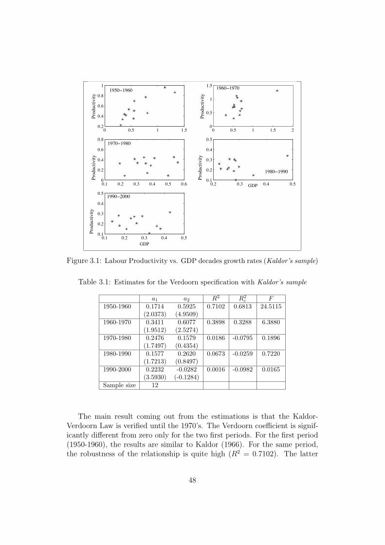
0 0.5 1 1.50.2
0.4
0.6
0.8
11950−1960
Productivity
0 0.5 1 1.5 20
0.5
1
1.5 1960−1970
Productivity
0.1 0.2 0.3 0.4 0.5 0.60
0.2
0.4
0.6
0.81970−1980
Productivity
0.2 0.3 0.4 0.50.1
0.2
0.3
0.4
0.5
1980−1990
GDP
Productivity
0.1 0.2 0.3 0.4 0.50.1
0.2
0.3
0.4
0.51990−2000
GDP
Productivity
Figure 3.1: Labour Productivity vs. GDP decades growth rates (Kaldor’s sample)
Table 3.1: Estimates for the Verdoorn specification with Kaldor’s sample
a1 a2 R2 R2c F
1950-1960 0.1714 0.5925 0.7102 0.6813 24.5115(2.0373) (4.9509)
1960-1970 0.3411 0.6077 0.3898 0.3288 6.3880(1.9512) (2.5274)
1970-1980 0.2476 0.1579 0.0186 -0.0795 0.1896(1.7497) (0.4354)
1980-1990 0.1577 0.2620 0.0673 -0.0259 0.7220(1.7213) (0.8497)
1990-2000 0.2232 -0.0282 0.0016 -0.0982 0.0165(3.5930) (-0.1284)
Sample size 12
The main result coming out from the estimations is that the Kaldor-Verdoorn Law is verified until the 1970’s. The Verdoorn coefficient is signif-icantly different from zero only for the two first periods. For the first period(1950-1960), the results are similar to Kaldor (1966). For the same period,the robustness of the relationship is quite high (R2 = 0.7102). The latter
48
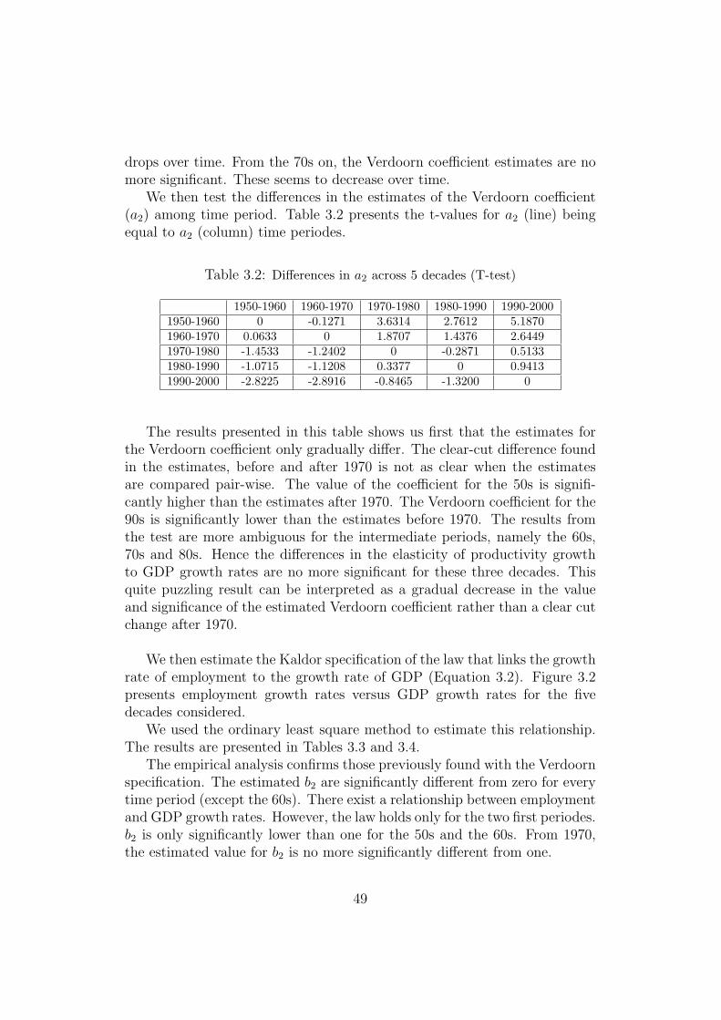
drops over time. From the 70s on, the Verdoorn coefficient estimates are nomore significant. These seems to decrease over time.
We then test the differences in the estimates of the Verdoorn coefficient(a2) among time period. Table 3.2 presents the t-values for a2 (line) beingequal to a2 (column) time periodes.
Table 3.2: Differences in a2 across 5 decades (T-test)
1950-1960 1960-1970 1970-1980 1980-1990 1990-20001950-1960 0 -0.1271 3.6314 2.7612 5.18701960-1970 0.0633 0 1.8707 1.4376 2.64491970-1980 -1.4533 -1.2402 0 -0.2871 0.51331980-1990 -1.0715 -1.1208 0.3377 0 0.94131990-2000 -2.8225 -2.8916 -0.8465 -1.3200 0
The results presented in this table shows us first that the estimates forthe Verdoorn coefficient only gradually differ. The clear-cut difference foundin the estimates, before and after 1970 is not as clear when the estimatesare compared pair-wise. The value of the coefficient for the 50s is signifi-cantly higher than the estimates after 1970. The Verdoorn coefficient for the90s is significantly lower than the estimates before 1970. The results fromthe test are more ambiguous for the intermediate periods, namely the 60s,70s and 80s. Hence the differences in the elasticity of productivity growthto GDP growth rates are no more significant for these three decades. Thisquite puzzling result can be interpreted as a gradual decrease in the valueand significance of the estimated Verdoorn coefficient rather than a clear cutchange after 1970.
We then estimate the Kaldor specification of the law that links the growthrate of employment to the growth rate of GDP (Equation 3.2). Figure 3.2presents employment growth rates versus GDP growth rates for the fivedecades considered.
We used the ordinary least square method to estimate this relationship.The results are presented in Tables 3.3 and 3.4.
The empirical analysis confirms those previously found with the Verdoornspecification. The estimated b2 are significantly different from zero for everytime period (except the 60s). There exist a relationship between employmentand GDP growth rates. However, the law holds only for the two first periodes.b2 is only significantly lower than one for the 50s and the 60s. From 1970,the estimated value for b2 is no more significantly different from one.
49
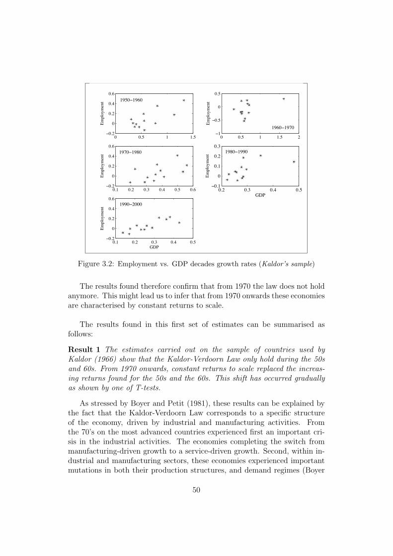
0 0.5 1 1.5−0.2
0
0.2
0.4
0.6
1950−1960Employment
0 0.5 1 1.5 2−1
−0.5
0
0.5
1960−1970
Employment
0.1 0.2 0.3 0.4 0.5 0.6−0.2
0
0.2
0.4
0.61970−1980
Employment
0.2 0.3 0.4 0.5−0.1
0
0.1
0.2
0.31980−1990
GDP
Employment
0.1 0.2 0.3 0.4 0.5−0.2
0
0.2
0.4
0.61990−2000
GDP
Employment
Figure 3.2: Employment vs. GDP decades growth rates (Kaldor’s sample)
The results found therefore confirm that from 1970 the law does not holdanymore. This might lead us to infer that from 1970 onwards these economiesare characterised by constant returns to scale.
The results found in this first set of estimates can be summarised asfollows:
Result 1 The estimates carried out on the sample of countries used byKaldor (1966) show that the Kaldor-Verdoorn Law only hold during the 50sand 60s. From 1970 onwards, constant returns to scale replaced the increas-ing returns found for the 50s and the 60s. This shift has occurred graduallyas shown by one of T-tests.
As stressed by Boyer and Petit (1981), these results can be explained bythe fact that the Kaldor-Verdoorn Law corresponds to a specific structureof the economy, driven by industrial and manufacturing activities. Fromthe 70’s on the most advanced countries experienced first an important cri-sis in the industrial activities. The economies completing the switch frommanufacturing-driven growth to a service-driven growth. Second, within in-dustrial and manufacturing sectors, these economies experienced importantmutations in both their production structures, and demand regimes (Boyer
50
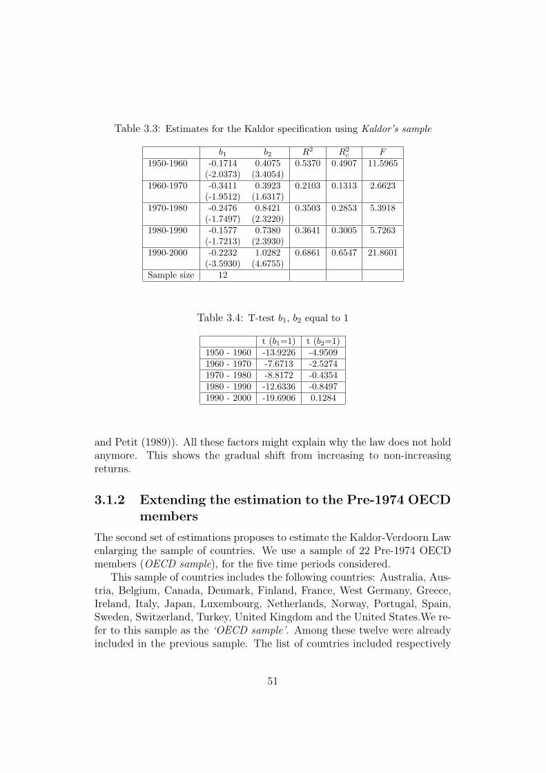
Table 3.3: Estimates for the Kaldor specification using Kaldor’s sample
b1 b2 R2 R2c F
1950-1960 -0.1714 0.4075 0.5370 0.4907 11.5965(-2.0373) (3.4054)
1960-1970 -0.3411 0.3923 0.2103 0.1313 2.6623(-1.9512) (1.6317)
1970-1980 -0.2476 0.8421 0.3503 0.2853 5.3918(-1.7497) (2.3220)
1980-1990 -0.1577 0.7380 0.3641 0.3005 5.7263(-1.7213) (2.3930)
1990-2000 -0.2232 1.0282 0.6861 0.6547 21.8601(-3.5930) (4.6755)
Sample size 12
Table 3.4: T-test b1, b2 equal to 1
t (b1=1) t (b2=1)1950 - 1960 -13.9226 -4.95091960 - 1970 -7.6713 -2.52741970 - 1980 -8.8172 -0.43541980 - 1990 -12.6336 -0.84971990 - 2000 -19.6906 0.1284
and Petit (1989)). All these factors might explain why the law does not holdanymore. This shows the gradual shift from increasing to non-increasingreturns.
3.1.2 Extending the estimation to the Pre-1974 OECDmembers
The second set of estimations proposes to estimate the Kaldor-Verdoorn Lawenlarging the sample of countries. We use a sample of 22 Pre-1974 OECDmembers (OECD sample), for the five time periods considered.
This sample of countries includes the following countries: Australia, Aus-tria, Belgium, Canada, Denmark, Finland, France, West Germany, Greece,Ireland, Italy, Japan, Luxembourg, Netherlands, Norway, Portugal, Spain,Sweden, Switzerland, Turkey, United Kingdom and the United States.We re-fer to this sample as the ‘OECD sample’. Among these twelve were alreadyincluded in the previous sample. The list of countries included respectively
51
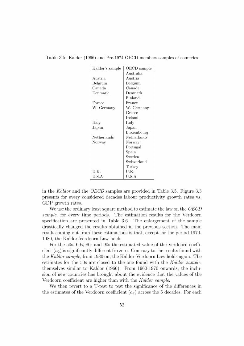
Table 3.5: Kaldor (1966) and Pre-1974 OECD members samples of countries
Kaldor’s sample OECD sampleAustralia
Austria AustriaBelgium BelgiumCanada CanadaDenmark Denmark
FinlandFrance FranceW. Germany W. Germany
GreeceIreland
Italy ItalyJapan Japan
LuxembourgNetherlands NetherlandsNorway Norway
PortugalSpainSwedenSwitzerlandTurkey
U.K. U.K.U.S.A U.S.A
in the Kaldor and the OECD samples are provided in Table 3.5. Figure 3.3presents for every considered decades labour productivity growth rates vs.GDP growth rates.
We use the ordinary least square method to estimate the law on the OECDsample, for every time periods. The estimation results for the Verdoornspecification are presented in Table 3.6. The enlargement of the sampledrastically changed the results obtained in the previous section. The mainresult coming out from these estimations is that, except for the period 1970-1980, the Kaldor-Verdoorn Law holds.
For the 50s, 60s, 80s and 90s the estimated value of the Verdoorn coeffi-cient (a2) is significantly different fro zero. Contrary to the results found withthe Kaldor sample, from 1980 on, the Kaldor-Verdoorn Law holds again. Theestimates for the 50s are closed to the one found with the Kaldor sample,themselves similar to Kaldor (1966). From 1960-1970 onwards, the inclu-sion of new countries has brought about the evidence that the values of theVerdoorn coefficient are higher than with the Kaldor sample.
We then revert to a T-test to test the significance of the differences inthe estimates of the Verdoorn coefficient (a2) across the 5 decades. For each
52
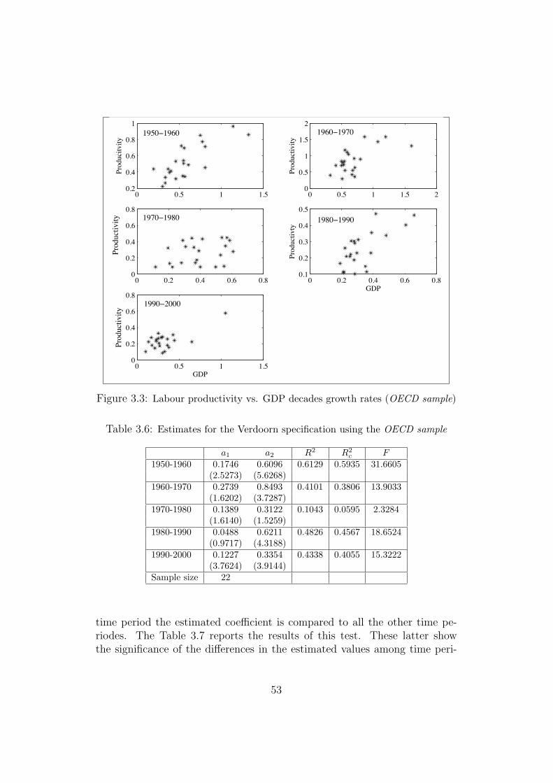
0 0.5 1 1.50.2
0.4
0.6
0.8
11950−1960
Producitvity
0 0.5 1 1.5 20
0.5
1
1.5
21960−1970
Productivity
0 0.2 0.4 0.6 0.80
0.2
0.4
0.6
0.81970−1980
Productivity
0 0.2 0.4 0.6 0.80.1
0.2
0.3
0.4
0.5
1980−1990
GDPProductivty
0 0.5 1 1.50
0.2
0.4
0.6
0.81990−2000
GDP
Productivity
Figure 3.3: Labour productivity vs. GDP decades growth rates (OECD sample)
Table 3.6: Estimates for the Verdoorn specification using the OECD sample
a1 a2 R2 R2c F
1950-1960 0.1746 0.6096 0.6129 0.5935 31.6605(2.5273) (5.6268)
1960-1970 0.2739 0.8493 0.4101 0.3806 13.9033(1.6202) (3.7287)
1970-1980 0.1389 0.3122 0.1043 0.0595 2.3284(1.6140) (1.5259)
1980-1990 0.0488 0.6211 0.4826 0.4567 18.6524(0.9717) (4.3188)
1990-2000 0.1227 0.3354 0.4338 0.4055 15.3222(3.7624) (3.9144)
Sample size 22
time period the estimated coefficient is compared to all the other time pe-riodes. The Table 3.7 reports the results of this test. These latter showthe significance of the differences in the estimated values among time peri-
53
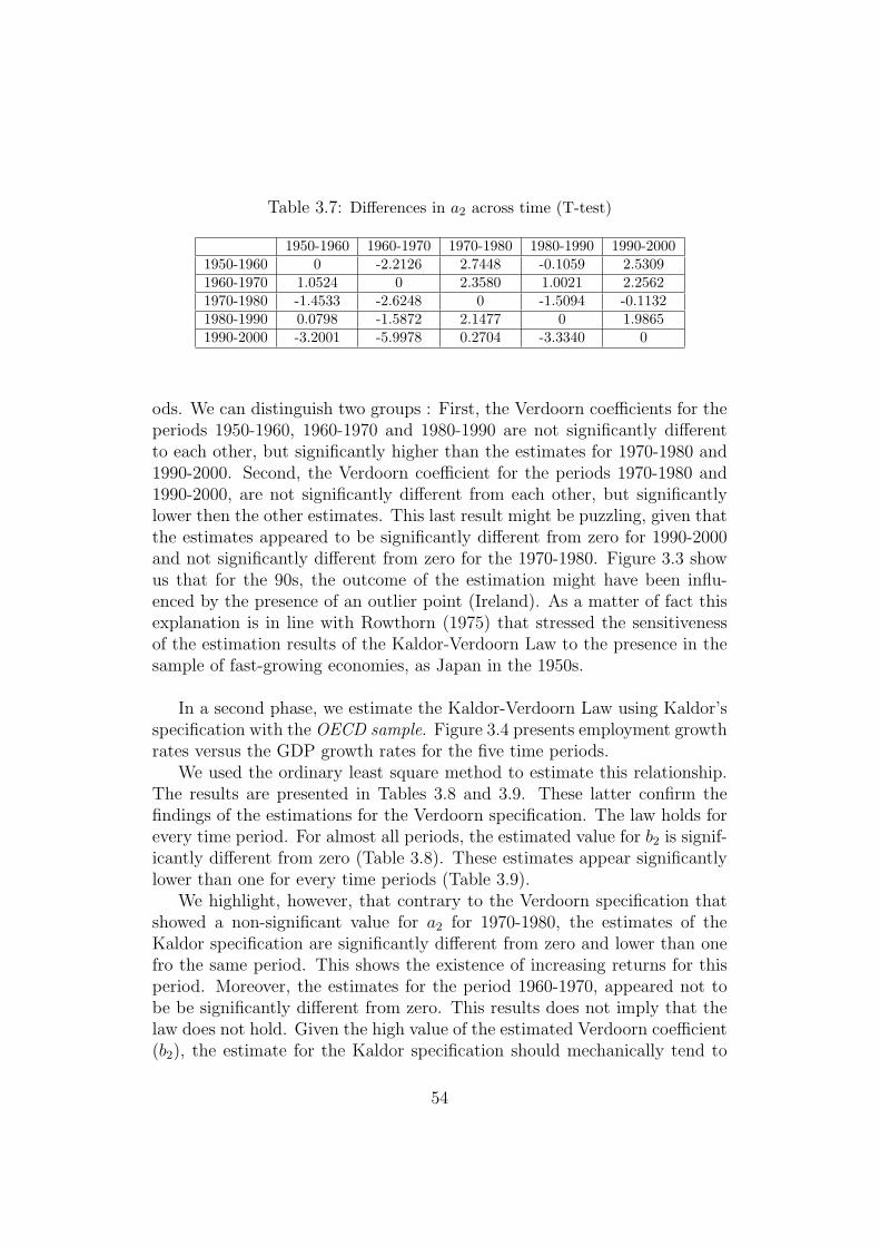
Table 3.7: Differences in a2 across time (T-test)
1950-1960 1960-1970 1970-1980 1980-1990 1990-20001950-1960 0 -2.2126 2.7448 -0.1059 2.53091960-1970 1.0524 0 2.3580 1.0021 2.25621970-1980 -1.4533 -2.6248 0 -1.5094 -0.11321980-1990 0.0798 -1.5872 2.1477 0 1.98651990-2000 -3.2001 -5.9978 0.2704 -3.3340 0
ods. We can distinguish two groups : First, the Verdoorn coefficients for theperiods 1950-1960, 1960-1970 and 1980-1990 are not significantly differentto each other, but significantly higher than the estimates for 1970-1980 and1990-2000. Second, the Verdoorn coefficient for the periods 1970-1980 and1990-2000, are not significantly different from each other, but significantlylower then the other estimates. This last result might be puzzling, given thatthe estimates appeared to be significantly different from zero for 1990-2000and not significantly different from zero for the 1970-1980. Figure 3.3 showus that for the 90s, the outcome of the estimation might have been influ-enced by the presence of an outlier point (Ireland). As a matter of fact thisexplanation is in line with Rowthorn (1975) that stressed the sensitivenessof the estimation results of the Kaldor-Verdoorn Law to the presence in thesample of fast-growing economies, as Japan in the 1950s.
In a second phase, we estimate the Kaldor-Verdoorn Law using Kaldor’sspecification with the OECD sample. Figure 3.4 presents employment growthrates versus the GDP growth rates for the five time periods.
We used the ordinary least square method to estimate this relationship.The results are presented in Tables 3.8 and 3.9. These latter confirm thefindings of the estimations for the Verdoorn specification. The law holds forevery time period. For almost all periods, the estimated value for b2 is signif-icantly different from zero (Table 3.8). These estimates appear significantlylower than one for every time periods (Table 3.9).
We highlight, however, that contrary to the Verdoorn specification thatshowed a non-significant value for a2 for 1970-1980, the estimates of theKaldor specification are significantly different from zero and lower than onefro the same period. This shows the existence of increasing returns for thisperiod. Moreover, the estimates for the period 1960-1970, appeared not tobe be significantly different from zero. This results does not imply that thelaw does not hold. Given the high value of the estimated Verdoorn coefficient(b2), the estimate for the Kaldor specification should mechanically tend to
54
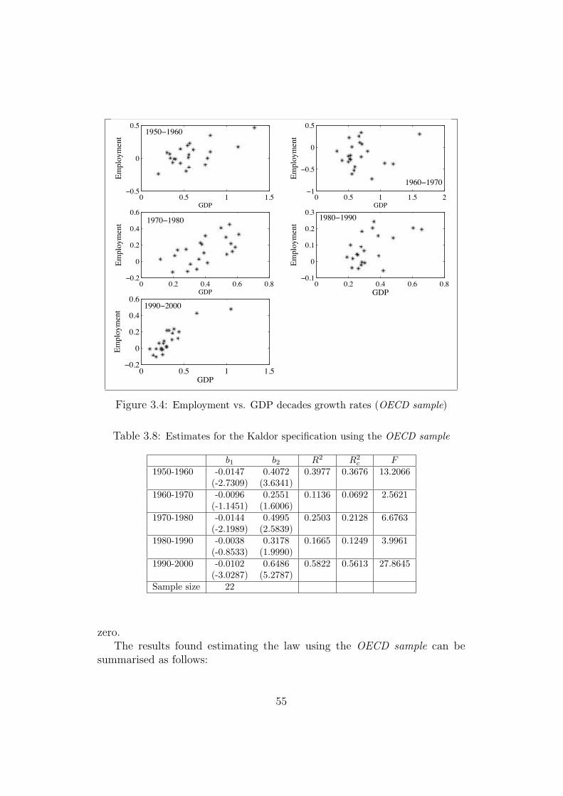
0 0.5 1 1.5−0.5
0
0.51950−1960
Employment
GDP0 0.5 1 1.5 2
−1
−0.5
0
0.5
1960−1970
GDP
Employment
0 0.2 0.4 0.6 0.8−0.2
0
0.2
0.4
0.61970−1980
GDP
Employment
0 0.2 0.4 0.6 0.8−0.1
0
0.1
0.2
0.31980−1990
GDPEmployment
0 0.5 1 1.5−0.2
0
0.2
0.4
0.61990−2000
GDP
Employment
Figure 3.4: Employment vs. GDP decades growth rates (OECD sample)
Table 3.8: Estimates for the Kaldor specification using the OECD sample
b1 b2 R2 R2c F
1950-1960 -0.0147 0.4072 0.3977 0.3676 13.2066(-2.7309) (3.6341)
1960-1970 -0.0096 0.2551 0.1136 0.0692 2.5621(-1.1451) (1.6006)
1970-1980 -0.0144 0.4995 0.2503 0.2128 6.6763(-2.1989) (2.5839)
1980-1990 -0.0038 0.3178 0.1665 0.1249 3.9961(-0.8533) (1.9990)
1990-2000 -0.0102 0.6486 0.5822 0.5613 27.8645(-3.0287) (5.2787)
Sample size 22
zero.The results found estimating the law using the OECD sample can be
summarised as follows:
55
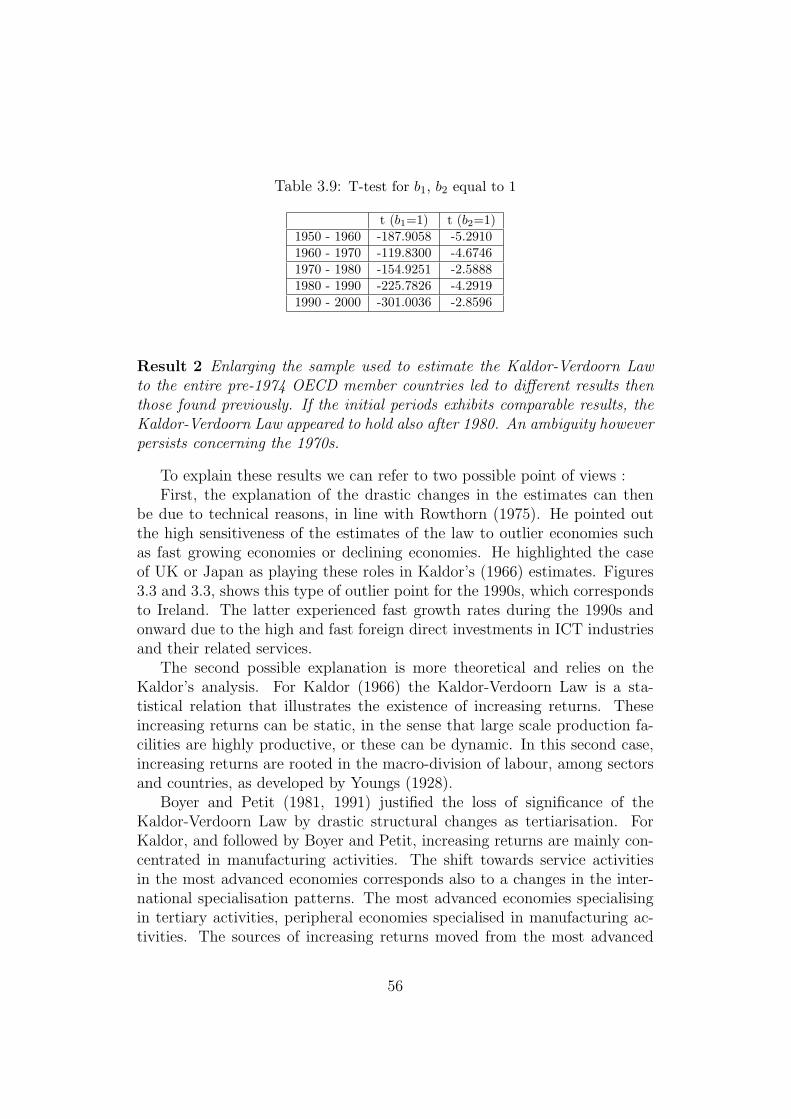
Table 3.9: T-test for b1, b2 equal to 1
t (b1=1) t (b2=1)1950 - 1960 -187.9058 -5.29101960 - 1970 -119.8300 -4.67461970 - 1980 -154.9251 -2.58881980 - 1990 -225.7826 -4.29191990 - 2000 -301.0036 -2.8596
Result 2 Enlarging the sample used to estimate the Kaldor-Verdoorn Lawto the entire pre-1974 OECD member countries led to different results thenthose found previously. If the initial periods exhibits comparable results, theKaldor-Verdoorn Law appeared to hold also after 1980. An ambiguity howeverpersists concerning the 1970s.
To explain these results we can refer to two possible point of views :First, the explanation of the drastic changes in the estimates can then
be due to technical reasons, in line with Rowthorn (1975). He pointed outthe high sensitiveness of the estimates of the law to outlier economies suchas fast growing economies or declining economies. He highlighted the caseof UK or Japan as playing these roles in Kaldor’s (1966) estimates. Figures3.3 and 3.3, shows this type of outlier point for the 1990s, which correspondsto Ireland. The latter experienced fast growth rates during the 1990s andonward due to the high and fast foreign direct investments in ICT industriesand their related services.
The second possible explanation is more theoretical and relies on theKaldor’s analysis. For Kaldor (1966) the Kaldor-Verdoorn Law is a sta-tistical relation that illustrates the existence of increasing returns. Theseincreasing returns can be static, in the sense that large scale production fa-cilities are highly productive, or these can be dynamic. In this second case,increasing returns are rooted in the macro-division of labour, among sectorsand countries, as developed by Youngs (1928).
Boyer and Petit (1981, 1991) justified the loss of significance of theKaldor-Verdoorn Law by drastic structural changes as tertiarisation. ForKaldor, and followed by Boyer and Petit, increasing returns are mainly con-centrated in manufacturing activities. The shift towards service activitiesin the most advanced economies corresponds also to a changes in the inter-national specialisation patterns. The most advanced economies specialisingin tertiary activities, peripheral economies specialised in manufacturing ac-tivities. The sources of increasing returns moved from the most advanced
56
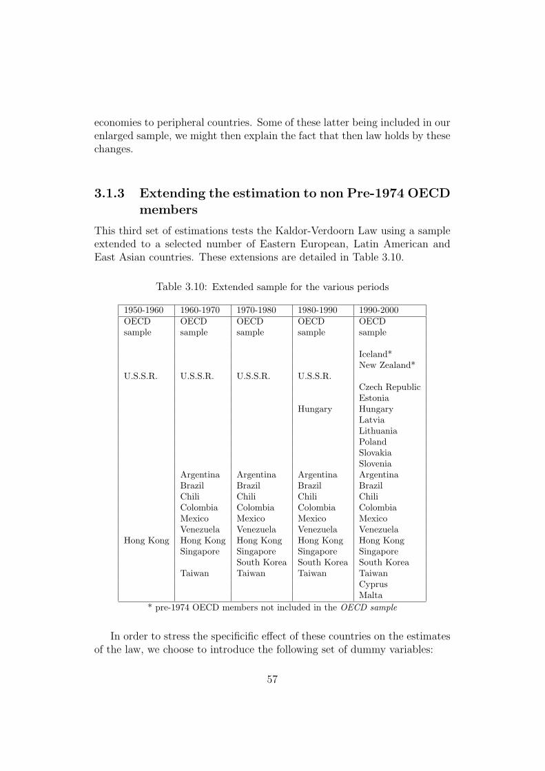
economies to peripheral countries. Some of these latter being included in ourenlarged sample, we might then explain the fact that then law holds by thesechanges.
3.1.3 Extending the estimation to non Pre-1974 OECDmembers
This third set of estimations tests the Kaldor-Verdoorn Law using a sampleextended to a selected number of Eastern European, Latin American andEast Asian countries. These extensions are detailed in Table 3.10.
Table 3.10: Extended sample for the various periods
1950-1960 1960-1970 1970-1980 1980-1990 1990-2000OECD OECD OECD OECD OECDsample sample sample sample sample
Iceland*New Zealand*
U.S.S.R. U.S.S.R. U.S.S.R. U.S.S.R.Czech RepublicEstonia
Hungary HungaryLatviaLithuaniaPolandSlovakiaSlovenia
Argentina Argentina Argentina ArgentinaBrazil Brazil Brazil BrazilChili Chili Chili ChiliColombia Colombia Colombia ColombiaMexico Mexico Mexico MexicoVenezuela Venezuela Venezuela Venezuela
Hong Kong Hong Kong Hong Kong Hong Kong Hong KongSingapore Singapore Singapore Singapore
South Korea South Korea South KoreaTaiwan Taiwan Taiwan Taiwan
CyprusMalta
* pre-1974 OECD members not included in the OECD sample
In order to stress the specificific effect of these countries on the estimatesof the law, we choose to introduce the following set of dummy variables:
57
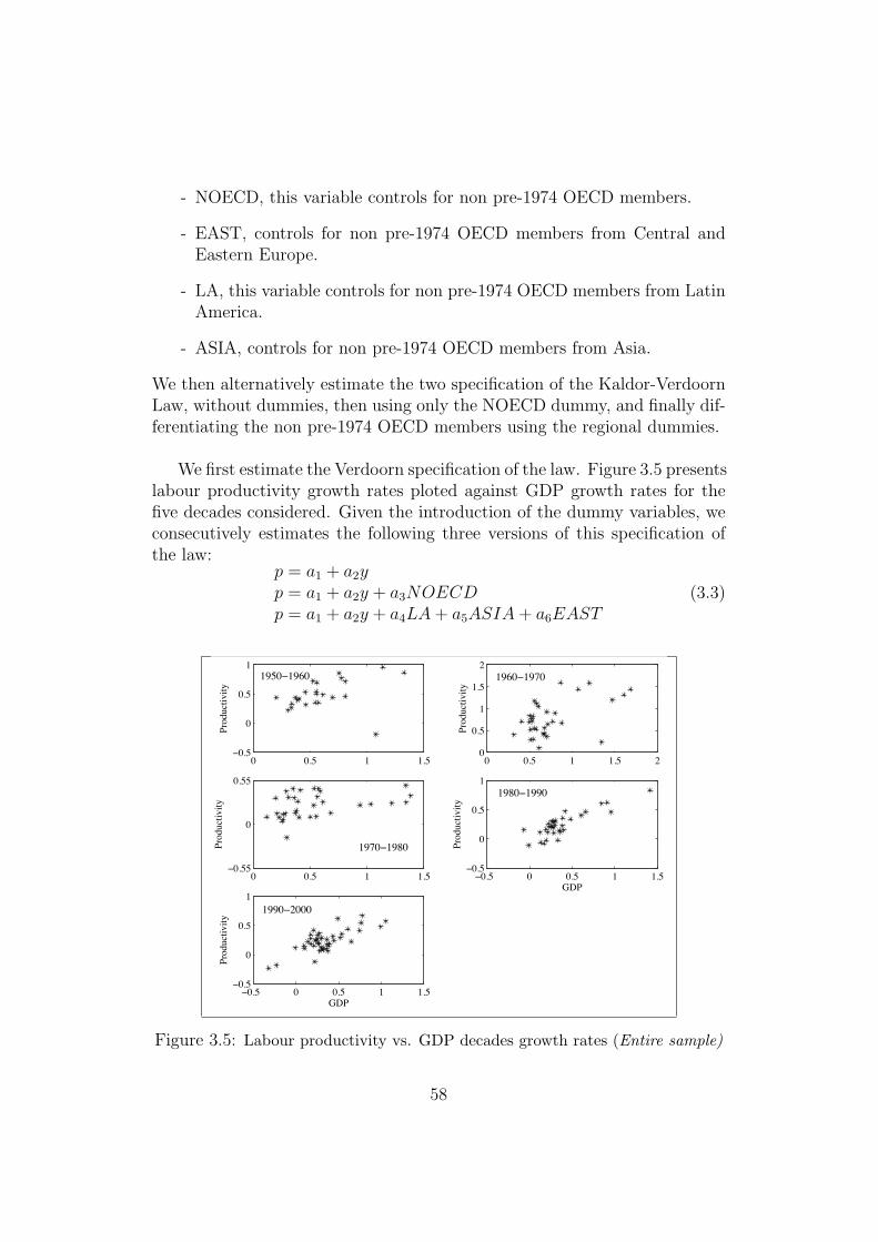
- NOECD, this variable controls for non pre-1974 OECD members.
- EAST, controls for non pre-1974 OECD members from Central andEastern Europe.
- LA, this variable controls for non pre-1974 OECD members from LatinAmerica.
- ASIA, controls for non pre-1974 OECD members from Asia.
We then alternatively estimate the two specification of the Kaldor-VerdoornLaw, without dummies, then using only the NOECD dummy, and finally dif-ferentiating the non pre-1974 OECD members using the regional dummies.
We first estimate the Verdoorn specification of the law. Figure 3.5 presentslabour productivity growth rates ploted against GDP growth rates for thefive decades considered. Given the introduction of the dummy variables, weconsecutively estimates the following three versions of this specification ofthe law:
p = a1 + a2yp = a1 + a2y + a3NOECDp = a1 + a2y + a4LA + a5ASIA + a6EAST
(3.3)
0 0.5 1 1.5−0.5
0
0.5
1
Productivity
1950−1960
0 0.5 1 1.5 20
0.5
1
1.5
2
Productivity
1960−1970
0 0.5 1 1.5−0.55
0
0.55
Productivity
1970−1980
−0.5 0 0.5 1 1.5−0.5
0
0.5
1
GDP
Productivity
1980−1990
−0.5 0 0.5 1 1.5−0.5
0
0.5
1
GDP
Productivity
1990−2000
Figure 3.5: Labour productivity vs. GDP decades growth rates (Entire sample)
58
We used the ordinary least square methode to estimate the three rela-tionship for each time period. The results of these estimations are presentedin Table 3.11.
The main result coming out from these estimations for almost all peri-ods (1960-1970, 1970-1980, 1980-1990 and 1990-2000), the Kaldor-VerdoornLaw holds for all the specification, including the dummy variables or thealternative one. For the 50s, the estimated value for the Verdoorn coeffi-cient appears not significant when the relationship is estimated without thedummy variable for the non pre-1974 OECD members. Once the dummyis introduced, the Kaldor-Verdoorn Law holds, the coefficient being signifi-cantly different from zero. Moreover its value, appears to be slightly smallerthan the estimates using the Kaldor sample and the OECD sample.
For all the periods until the 90s, the estimated value for the Verdoorncoefficient are similar to the estimated values realised with the two othersamples, when the dummy variables are introduced. In other words, theenlargement to non OECD members does not seem to affect the value of theVerdoorn parameter.
59
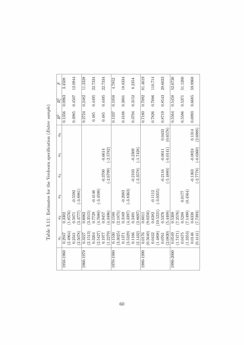
Tab
le3.
11:
Est
imat
esfo
rth
eV
erdo
orn
spec
ifica
tion
(Ent
ire
sam
ple)
a1
a2
a3
a4
a5
a6
R2
R2 c
F19
50-1
960
0.29
470.
3302
0.13
560.
0963
3.45
08(2
.496
4)(1
.857
6)0.
2341
0.50
71-0
.559
20.
4985
0.45
0712
.094
4(2
.507
8)(3
.477
7)(-
3.89
81)
1960
-197
00.
3227
0.60
620.
2724
0.24
8211
.232
8(2
.151
3)(3
.351
5)0.
3264
0.77
29-0
.414
60.
485
0.44
9522
.733
4(2
.542
7)(4
.768
0)(-
3.45
98)
0.19
770.
9457
-0.3
700
-0.6
614
0.48
50.
4495
22.7
334
(1.2
279)
(4.3
496)
(-2.
6799
)(-
2.57
82)
1970
-198
00.
1530
0.15
800.
1337
0.10
584.
7852
(3.3
025)
(2.1
875)
0.13
710.
3169
-0.2
083
0.41
880.
3801
18.8
334
(3.5
329)
(4.3
397)
(-3.
8363
)0.
1166
0.34
91-0
.210
3-0
.230
90.
3794
0.31
528.
2354
(2.1
432)
(2.8
697)
(-3.
3578
)(-
1.74
28)
1980
-199
00.
0176
0.60
110.
7180
0.70
9281
.461
9(0
.564
0)(9
.025
6)0.
0432
0.63
82-0
.111
20.
7826
0.76
8611
0.71
4(1
.480
8)(1
0.52
21)
(-3.
0355
)0.
0761
0.53
76-0
.211
6-0
.001
10.
0433
0.87
190.
8543
29.6
023
(2.0
830)
(5.4
408)
(-5.
4880
)(-
0.01
41)
(0.6
578)
1990
-200
00.
0549
0.53
080.
5564
0.54
5852
.672
6(1
.747
1)(7
.257
6)0.
0475
0.52
880.
0177
0.55
860.
5371
51.1
200
(1.3
353)
(7.1
498)
(0.4
564)
0.01
460.
6338
-0.1
363
-0.0
024
0.13
140.
6993
0.66
8559
.896
8(0
.414
1)(7
.739
3)(-
2.77
78)
(-0.
0360
)(2
.698
8)
60
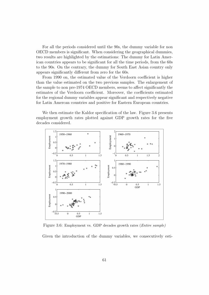
For all the periods considered until the 90s, the dummy variable for nonOECD members is significant. When considering the geographical dummies,two results are highlighted by the estimations: The dummy for Latin Amer-ican countries appears to be significant for all the time periods, from the 60sto the 90s. On the contrary, the dummy for South East Asian country onlyappears significantly different from zero for the 60s.
From 1990 on, the estimated value of the Verdoorn coefficient is higherthan the value estimated on the two previous samples. The enlargement ofthe sample to non pre-1974 OECD members, seems to affect significantly theestimates of the Verdoorn coefficient. Moreover, the coefficients estimatedfor the regional dummy variables appear significant and respectively negativefor Latin Amercan countries and positive for Eastern European countries.
We then estimate the Kaldor specification of the law. Figure 3.6 presentsemployment growth rates plotted against GDP growth rates for the fivedecades considered.
0 0.5 1 1.5−0.5
0
0.5
1
1.51950−1960
Employment
0 0.5 1 1.5 2−1
0
1
21960−1970
Employment
0 0.5 1 1.5−0.5
0
0.5
1
1.51970−1980
Employment
−0.5 0 0.5 1 1.5−0.5
0
0.5
1
1980−1990
GDP
Employment
−0.5 0 0.5 1 1.5−0.5
0
0.5
1
1990−2000
GDP
Employment
Figure 3.6: Employment vs. GDP decades growth rates (Entire sample)
Given the introduction of the dummy variables, we consecutively esti-
61
mates the following three versions of this specification of the law:
e = b1 + b2ye = b1 + b2y + b3NOECDe = b1 + b2y + b4LA + b5ASIA + b6EAST
(3.4)
We used the ordinary least square methode to estimate the three relation-ships for each time period. The results of these estimations are presented inTable 3.12.
The Kaldor’s specification of the relationship confirms the results foundpreviously. The estimates are such that the law holds for every time periods,when the dummy variables are included into the estimation. The estimatedvalue for the coefficient b2 appears to be significantly different from zero forall the periods except 1960-1970, and significantly lower then one for all thetime periods when the dummy is included. For the 60s, the fact that b2
appears not significantly different from zero is mechanically due to the factthat the estimated value of a2 tends to one.
The main results of the estimation realised using the extended sample ofcountries can be summarised as follows:
Result 3 Enlarging the sample used to estimate the Kaldor-Verdoorn Lawto a selected numbers of Eastern European, Latin American and South EastAsian countries, confirms that the Law holds at the macro-economic level.The estimated value of the Verdoorn coefficients appears similar to the oneestimated. The dummy for the non pre-1974 OECD countries appears to besignificant until the 90s. The dummy for Latin American countries remainssignificant over time, while for South East Asian it appears insignificant fromthe 70s on.
In this third case, the results can be explained in two ways: First, onceagain we can refer to Rowthorn (1975) ’s critic. The estimations can besensitive to the existence of outliers. In this case, the existence of an outlierpoint (Hong Kong) explains why the estimated values for the period 1950-1960 are not significant. This problem is however accounted for with theintroduction of the dummy variables.
The second explanation relies on the dynamic increasing returns. ForKaldor (1966), relying on Young (1928), the dynamic increasing returns arelinked to the division of labour across sectors. In this case again, the resultscan then be explained by the international division of labour and the real-location of manufacturing activities to peripheral countries. The fact thatthe dummy for South Asian countries is not significantly different from zerofrom the 70s onwards might confirms this interpretation.
62
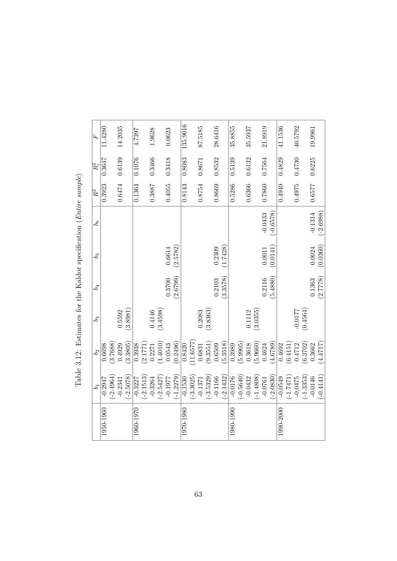
Tab
le3.
12:
Est
imat
esfo
rth
eK
aldo
rsp
ecifi
cati
on(E
ntire
sam
ple)
b 1b 2
b 3b 4
b 5b 6
R2
R2 c
F19
50-1
960
-0.2
947
0.66
980.
3923
0.36
4711
.428
0(-
2.49
64)
(3.7
688)
-0.2
341
0.49
290.
5592
0.64
740.
6139
14.2
035
(-2.
5078
)(3
.380
5)(3
.898
1)19
60-1
970
-0.3
227
0.39
380.
1364
0.10
764.
7397
(-2.
1513
)(2
.177
1)-0
.326
40.
2271
0.41
460.
3887
0.34
661.
9628
(-2.
5427
)(1
.401
0)(3
.459
8)-0
.197
70.
0543
0.37
000.
6614
0.40
550.
3418
0.06
23(-
1.22
79)
(0.2
496)
(2.6
799)
(2.5
782)
1970
-198
0-0
.153
00.
8420
0.81
430.
8083
135.
9016
(-3.
3025
)(1
1.65
77)
-0.1
371
0.68
310.
2083
0.87
540.
8671
87.5
185
(-3.
5329
)(9
.355
1)(3
.836
3)-0
.116
60.
6509
0.21
030.
2309
0.86
690.
8532
28.6
416
(-2.
1432
)(5
.351
8)(3
.357
8)(1
.742
8)19
80-1
990
-0.0
176
0.39
890.
5286
0.51
3935
.885
5(-
0.56
40)
(5.9
905)
-0.0
432
0.36
180.
1112
0.63
660.
6132
35.5
937
(-1.
4808
)(5
.966
0)(3
.035
5)-0
.076
10.
4624
0.21
160.
0011
-0.0
433
0.78
600.
7564
21.8
919
(-2.
0830
)(4
.678
9)(5
.488
0)(0
.014
1)(-
0.65
78)
1990
-200
0-0
.054
90.
4692
0.49
490.
4829
41.1
536
(-1.
7471
)(6
.415
1)-0
.047
50.
4712
-0.0
177
0.49
750.
4730
40.5
792
(-1.
3353
)(6
.370
2)(0
.456
4)-0
.014
60.
3662
0.13
630.
0024
-0.1
314
0.65
770.
6225
19.9
961
(-0.
4141
)(4
.471
7)(2
.777
8)(0
.036
0)(-
2.69
88)
63
To sum up the findings of the macro-level estimations of the Kaldor-Verdoorn Law. We can stress that if the Law does hold after 1970 whenestimated for a restricted sample of advanced economies, the latter is verifiedwhen estimated on the extended versions of the sample. This result can findan explanation in the drastic changes in the structures of the most advancedeconomies after 1970 and in the international reallocation of manufacturingactivities. The sources of increasing returns have then migrated to peripheralcountries.
3.2 A sectoral approach to the Kaldor-Verdoorn
Law.
The second section of this chapter proposes to estimate the Kaldor-VerdoornLaw at the sectoral level. We use cross-country estimations for a selectednumber of sectors over two periods, 1980-1990 and 1990-2000. Our sampleincludes 16 countries namely: Austria, Belgium, Denmark, Finland, France,Germany, Greece, Ireland, Italy, Luxembourg, Netherlands, Portugal, Spain,Sweden, UK and USA. We use this sample of countries to estimated theKaldor-Verdoorn Law for the 56 sectors detailed in Table 3.13.
As in the previous section we estimate the Kaldor-Verdoorn Law usingthe specifications:
- the Verdoorn specification:
p = a1 + a2y
- the Kaldor specification:e = b1 + b2y
where p, e, and y, respectively represents the growth rates of labour produc-tivity, employment, and real GDP.
Our data-set is built upon the October 2003, “Groningen Growth andDevelopment Center, 60-Industry Database”5. More specifically, we rely onthe “1995 constant prices value added” and the “Total employment in hours”series for the period 1979 to 2000 to compute the sector’s gross output,employment and labour productivity growth rates. The detailed data-setcan be found in appendix. We choose to estimate the Kaldor-Verdoorn Lawusing the decades’ growth rates. These are computed as the growth ratesbetween the average values over the two initial and the average over the twolast years of a given decade.
5The database is available at http://www.ggdc.net
64

Table 3.13: List of sectors
1 Agriculture 31 Furniture, miscellaneous manufacturing;2 Forestry recycling3 Fishing 32 Electricity, gas and water supply4 Mining and quarrying 33 Construction5 Food, drink & tobacco 34 Sale, maintenance, repair of motor6 Textiles vehicles; retail sale of automotive fuel7 Clothing 35 Wholesale trade and commission trade,8 Leather and footwear except of motor vehicles and motorcycles9 Wood & products of wood 36 Retail trade, except of motor vehicles;
and cork repair of personal and household goods10 Pulp, paper & paper products 37 Hotels & catering11 Printing & publishing 38 Inland transport12 Mineral oil refining, coke 39 Water transport
& nuclear fuel 40 Air transport13 Chemicals 41 Supporting and auxiliary transport14 Rubber & plastics activities; travel agencies15 Non-metallic mineral products 42 Communications16 Basic metals 43 Financial intermediation, except17 Fabricated metal products insurance and pension funding18 Mechanical engineering 44 Insurance and pension funding,19 Office machinery except compulsory social security20 Insulated wire 45 Activities auxiliary to financial21 Other electrical machinery intermediation
and apparatus nec 46 Real estate activities22 Electronic valves and tubes 47 Renting of machinery and equipment23 Telecommunication equipment 48 Computer and related activities24 Radio and television receivers 49 Research and development25 Scientific instruments 50 Legal, technical and advertising26 Other instruments 51 Other business activities, nec27 Motor vehicles 52 Public administration and defence;28 Building and repairing compulsory social security
of ships and boats 53 Education29 Aircraft and spacecraft 54 Health and social work30 Railroad equipment and 55 Other community, social and
transport equipment nec personal services56 Private households
with employed persons
We choose to realise these estimations , first, to test its reliability at themeso-level. Second, we aim to see whether the assertion made on the effectof structural change on the macro-estimates can be confirmed by the sectorallevel analysis. Finally we aim to stress the possible changes in the estimatesarising from one period to the other.
65
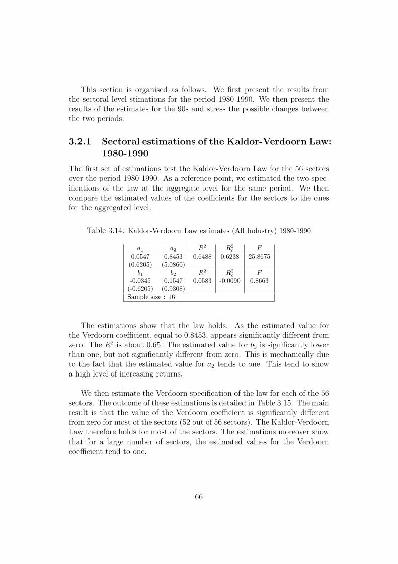
This section is organised as follows. We first present the results fromthe sectoral level stimations for the period 1980-1990. We then present theresults of the estimates for the 90s and stress the possible changes betweenthe two periods.
3.2.1 Sectoral estimations of the Kaldor-Verdoorn Law:1980-1990
The first set of estimations test the Kaldor-Verdoorn Law for the 56 sectorsover the period 1980-1990. As a reference point, we estimated the two spec-ifications of the law at the aggregate level for the same period. We thencompare the estimated values of the coefficients for the sectors to the onesfor the aggregated level.
Table 3.14: Kaldor-Verdoorn Law estimates (All Industry) 1980-1990
a1 a2 R2 R2c F
0.0547 0.8453 0.6488 0.6238 25.8675(0.6205) (5.0860)
b1 b2 R2 R2c F
-0.0345 0.1547 0.0583 -0.0090 0.8663(-0.6205) (0.9308)Sample size : 16
The estimations show that the law holds. As the estimated value forthe Verdoorn coefficient, equal to 0.8453, appears significantly different fromzero. The R2 is about 0.65. The estimated value for b2 is significantly lowerthan one, but not significantly different from zero. This is mechanically dueto the fact that the estimated value for a2 tends to one. This tend to showa high level of increasing returns.
We then estimate the Verdoorn specification of the law for each of the 56sectors. The outcome of these estimations is detailed in Table 3.15. The mainresult is that the value of the Verdoorn coefficient is significantly differentfrom zero for most of the sectors (52 out of 56 sectors). The Kaldor-VerdoornLaw therefore holds for most of the sectors. The estimations moreover showthat for a large number of sectors, the estimated values for the Verdoorncoefficient tend to one.
66
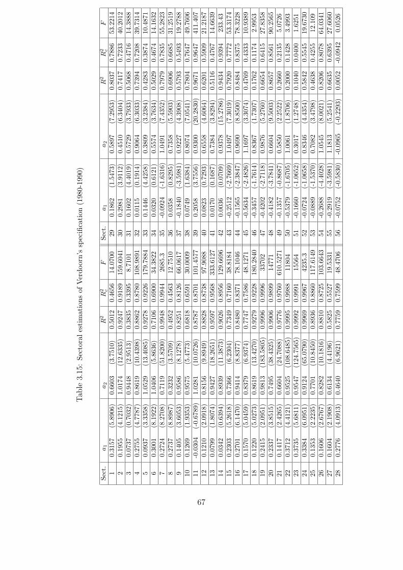
Tab
le3.
15:
Sect
oral
esti
mat
ions
ofV
erdo
orn’
ssp
ecifi
cati
on(1
980-
1990
)
Sect
.a1
a2
R2
R2 c
FSe
ct.
a1
a2
R2
R2 c
F1
0.31
57(5
.890
6)0.
6603
(3.7
510)
0.50
120.
4656
14.0
700
290.
1862
(1.5
473)
0.58
97(7
.295
3)0.
8037
0.78
8653
.221
42
0.19
55(4
.121
5)1.
0174
(12.
6335
)0.
9247
0.91
8915
9.60
4130
0.29
81(3
.911
2)0.
4510
(6.3
404)
0.74
170.
7233
40.2
012
30.
0737
(0.7
032)
0.94
48(2
.951
3)0.
3835
0.33
958.
7101
310.
1602
(4.4
019)
0.57
29(3
.793
3)0.
5068
0.47
1614
.388
84
0.27
55(4
.778
7)0.
8619
(10.
4398
)0.
8862
0.87
8010
8.98
9132
0.01
15(0
.191
4)0.
9064
(6.3
033)
0.73
940.
7208
39.7
314
50.
0937
(3.3
358)
1.05
29(1
3.40
85)
0.92
780.
9226
179.
7884
330.
1446
(4.4
258)
0.38
09(3
.238
4)0.
4283
0.38
7410
.487
16
0.30
01(8
.192
2)1.
0406
(5.8
636)
0.71
060.
6900
34.3
822
340.
0320
(0.6
121)
0.55
74(3
.763
4)0.
5029
0.46
7414
.163
27
0.27
24(8
.270
8)0.
7119
(51.
8200
)0.
9948
0.99
4426
85.3
35-0
.092
4(-
1.63
16)
1.04
91(7
.435
2)0.
7979
0.78
3555
.282
38
0.27
37(8
.898
7)0.
3232
(3.5
709)
0.49
520.
4563
12.7
510
360.
0358
(0.8
295)
0.73
58(5
.590
3)0.
6906
0.66
8531
.251
99
0.14
05(3
.605
3)0.
9586
(8.1
278)
0.82
510.
8126
66.0
617
37-0
.184
0(-
3.59
81)
0.92
27(4
.390
8)0.
5793
0.54
9319
.278
810
0.12
69(1
.935
3)0.
9575
(5.4
773)
0.68
180.
6591
30.0
009
380.
0749
(1.6
384)
0.80
74(7
.054
1)0.
7804
0.76
4749
.760
611
-0.0
304
(-0.
6789
)1.
0281
(10.
0726
)0.
8787
0.87
0110
1.45
7739
0.20
58(3
.755
6)0.
9300
(20.
2830
)0.
9671
0.96
4741
1.40
712
0.12
10(2
.091
8)0.
8156
(9.8
949)
0.88
280.
8738
97.9
088
400.
0823
(0.7
293)
0.65
58(4
.606
4)0.
6201
0.59
0921
.218
713
0.07
99(1
.807
4)0.
9427
(18.
2651
)0.
9597
0.95
6833
3.61
2741
0.01
70(0
.168
7)0.
7384
(3.8
294)
0.51
160.
4767
14.6
639
140.
0342
(0.6
394)
0.89
39(1
1.38
73)
0.90
260.
8956
129.
6696
420.
0036
(0.0
709)
0.93
78(1
5.27
86)
0.94
340.
9394
233.
4315
0.23
03(5
.261
8)0.
7366
(6.2
304)
0.73
490.
7160
38.8
184
43-0
.251
2(-
2.76
69)
1.04
97(7
.301
9)0.
7920
0.77
7253
.317
416
0.27
01(6
.147
0)0.
9414
(8.8
377)
0.84
800.
8371
78.1
046
44-0
.156
5(-
2.38
47)
0.96
90(8
.850
0)0.
8484
0.83
7578
.322
817
0.15
70(5
.045
9)0.
8379
(6.9
374)
0.77
470.
7586
48.1
271
45-0
.563
4(-
2.48
26)
1.16
97(3
.307
4)0.
4769
0.43
3310
.938
918
0.12
20(5
.027
3)0.
8619
(13.
4270
)0.
9279
0.92
2818
0.28
4046
-0.3
457
(-1.
7614
)0.
8367
(1.7
307)
0.17
620.
1174
2.99
5319
0.24
15(2
.095
1)0.
9813
(183
.580
5)0.
9996
0.99
9633
702
47-0
.420
2(-
2.71
18)
0.98
76(5
.276
0)0.
6654
0.64
1527
.835
820
0.23
37(3
.851
5)0.
7495
(38.
4325
)0.
9906
0.98
9914
771
48-0
.418
2(-
3.78
41)
0.66
04(9
.500
3)0.
8657
0.85
6190
.256
521
0.14
17(2
.426
5)0.
6604
(24.
7088
)0.
9776
0.97
6061
0.52
7149
-0.1
357
(-0.
8687
)0.
5850
(2.2
522)
0.26
600.
2135
5.07
2622
0.37
12(4
.412
1)0.
9525
(108
.648
5)0.
9995
0.99
8811
804
50-0
.537
9(-
1.67
05)
1.00
61(1
.870
6)0.
2000
0.14
283.
4993
230.
3735
(5.6
811)
0.95
47(1
24.7
565)
0.99
920.
9991
1556
451
-0.1
660
(-1.
0652
)0.
3017
(1.2
748)
0.10
400.
0400
1.62
5124
0.33
84(6
.095
1)0.
9124
(65.
0790
)0.
9969
0.99
6742
35.3
52-0
.072
4(-
1.06
58)
0.83
46(4
.435
4)0.
5842
0.55
4519
.673
025
0.13
53(2
.223
5)0.
7701
(10.
8450
)0.
8936
0.88
6011
7.61
4953
-0.0
889
(-1.
5370
)0.
7082
(3.4
798)
0.46
380.
4255
12.1
0926
0.16
06(2
.676
7)0.
8282
(10.
1816
)0.
8810
0.87
2510
3.66
4354
-0.2
688
(-4.
4028
)1.
0545
(8.0
021)
0.82
060.
8078
64.0
341
270.
1604
(2.1
908)
0.61
34(4
.419
6)0.
5825
0.55
2719
.533
155
-0.2
919
(-3.
5981
)1.
1813
(5.2
541)
0.66
350.
6395
27.6
060
280.
2776
(4.0
913)
0.46
40(6
.962
1)0.
7759
0.75
9948
.470
656
-0.0
752
(-0.
5830
)-0
.096
5(-
0.22
93)
0.00
52-0
.094
20.
0526
67
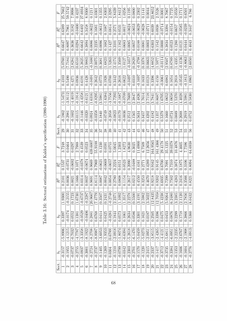
Tab
le3.
16:
Sect
oral
esti
mat
ions
ofK
aldo
r’s
spec
ifica
tion
(198
0-19
90)
Sect
.b 1
b 2R
2R
2 cF
Sect
.b 1
b 2R
2R
2 cF
1-0
.315
7(-
5.89
06)
0.33
97(1
.930
0)0.
2101
0.15
373.
7248
29-0
.186
2(-
1.54
73)
0.41
03(5
.076
0)0.
6647
0.63
8925
.766
22
-0.1
955
(-4.
1215
)-0
.017
4(-
0.21
55)
0.00
36-0
.073
10.
0464
30-0
.298
1(-
3.91
12)
0.54
90(7
.718
4)0.
8097
0.79
6159
.574
23
-0.0
737
(-0.
7032
)0.
0552
(0.1
723)
0.00
21-0
.069
20.
0297
31-0
.160
2(-
4.40
19)
0.42
71(2
.828
4)0.
3636
0.31
827.
9998
4-0
.275
5(-
4.77
87)
0.13
81(1
.673
0)0.
1666
0.10
712.
7988
32-0
.011
5(-
0.19
14)
0.09
36(0
.651
0)0.
0294
-0.0
400
0.42
375
-0.0
937
(-3.
3358
)-0
.052
9(-
0.67
37)
0.03
14-0
.037
80.
4539
33-0
.144
6(-
4.42
58)
0.61
91(5
.262
5)0.
6642
0.64
0227
.693
46
-0.3
001
(-8.
1922
)-0
.040
6(-
0.22
87)
0.00
37-0
.067
40.
0523
34-0
.032
0(-
0.61
21)
0.44
26(2
.988
3)0.
3894
0.34
588.
9300
7-0
.272
4(-
8.27
08)
0.28
81(2
0.96
67)
0.96
910.
9669
439.
6007
350.
0924
(1.6
316)
-0.0
491
(-0.
3480
)0.
0086
-0.0
622
0.12
118
-0.2
737
(-8.
8987
)0.
6768
(7.4
779)
0.81
140.
7969
55.9
188
36-0
.035
8(-
0.82
95)
0.26
42(2
.007
5)0.
2235
0.16
814.
0301
9-0
.140
5(-
3.60
53)
0.04
14(0
.350
7)0.
0087
-0.0
621
0.12
3037
0.18
40(3
.598
1)0.
0773
(0.3
681)
0.00
96-0
.061
20.
1355
10-0
.126
9(-
1.93
53)
0.04
25(0
.243
1)0.
0042
-0.0
669
0.05
9138
-0.0
749
(-1.
6384
)0.
1926
(1.6
823)
0.16
820.
1087
2.83
0311
0.03
04(0
.678
9)-0
.028
1(-
0.27
48)
0.00
54-0
.065
70.
0755
39-0
.205
8(-
3.75
56)
0.07
00(1
.526
3)0.
1427
0.08
142.
3295
12-0
.121
0(-
2.09
18)
0.18
44(2
.237
1)0.
2780
0.22
245.
0045
40-0
.082
3(-
0.72
93)
0.34
42(2
.417
4)0.
3101
0.25
715.
8439
13-0
.079
9(-
1.80
74)
0.05
73(1
.109
2)0.
0808
0.01
511.
2303
41-0
.017
0(-
0.16
87)
0.26
16(1
.356
9)0.
1162
0.05
311.
8412
14-0
.034
2(-
0.63
94)
0.10
61(1
.351
7)0.
1154
0.05
231.
8272
42-0
.003
6(-
0.07
09)
0.06
22(1
.012
7)0.
0683
0.00
171.
0256
15-0
.230
3(-
5.26
18)
0.26
34(2
.227
8)0.
2617
0.20
904.
9630
430.
2512
(2.7
669)
-0.0
497
(-0.
3457
)0.
0085
-0.0
624
0.11
9516
-0.2
701
(-6.
1470
)0.
0586
(0.5
500)
0.02
12-0
.048
80.
3025
440.
1565
(2.3
847)
0.03
10(0
.282
9)0.
0057
-0.0
653
0.08
0017
-0.1
570
(-5.
0459
)0.
3301
(3.4
191)
0.45
500.
4161
11.6
900
450.
5634
(2.4
826)
-0.1
697
(-0.
4798
)0.
0188
-0.0
629
0.23
0218
-0.1
220
(-5.
0273
)0.
1621
(2.5
982)
0.32
530.
2771
6.75
0946
0.34
57(1
.761
4)0.
1633
(0.3
378)
0.00
81-0
.062
80.
1141
19-0
.241
5(-
2.09
51)
0.01
87(3
.502
2)0.
4670
0.42
8912
.265
647
0.42
02(2
.711
8)0.
0124
(0.0
663)
0.00
03-0
.071
10.
0044
20-0
.233
7(-
3.85
15)
0.25
05(1
2.84
35)
0.92
180.
9162
164.
9565
480.
4182
(3.7
841)
0.33
96(4
.885
2)0.
6303
0.60
3923
.865
221
-0.1
417
(-2.
4265
)0.
3396
(12.
7058
)0.
9202
0.91
4516
1.43
6649
0.13
57(0
.868
7)0.
4150
(1.5
977)
0.15
420.
0938
2.55
2622
-0.3
712
(-4.
4121
)0.
0475
(5.4
238)
0.69
350.
6700
29.4
178
500.
5379
(1.6
705)
-0.0
061
(-0.
0114
)0.
0000
-0.0
714
0.00
0123
-0.3
735
(-5.
6811
)0.
0453
(5.9
264)
0.72
990.
7091
35.1
225
510.
1660
(1.0
652)
0.69
83(2
.950
7)0.
3834
0.33
948.
7067
24-0
.338
4(-
6.09
51)
0.08
76(6
.248
0)0.
7502
0.73
1039
.037
852
0.07
24(1
.065
8)0.
1654
(0.8
789)
0.05
23-0
.015
40.
7725
25-0
.135
3(-
2.22
35)
0.22
99(3
.238
5)0.
4283
0.38
7410
.487
653
0.08
89(1
.537
0)0.
2918
(1.4
335)
0.12
800.
0657
2.05
5026
-0.1
606
(-2.
6767
)0.
1718
(2.1
120)
0.24
160.
1875
4.46
0554
0.26
88(4
.402
8)-0
.054
5(-
0.41
36)
0.01
21-0
.058
50.
1711
27-0
.160
4(-
2.19
08)
0.38
66(2
.785
6)0.
3566
0.31
067.
7596
550.
2919
(3.5
981)
-0.1
813
(-0.
8063
)0.
0444
-0.0
239
0.65
0128
-0.2
776
(-4.
0913
)0.
5360
(8.0
432)
0.82
210.
8094
64.6
938
560.
0752
(0.5
830)
1.09
65(2
.605
0)0.
4043
0.34
476.
786
68
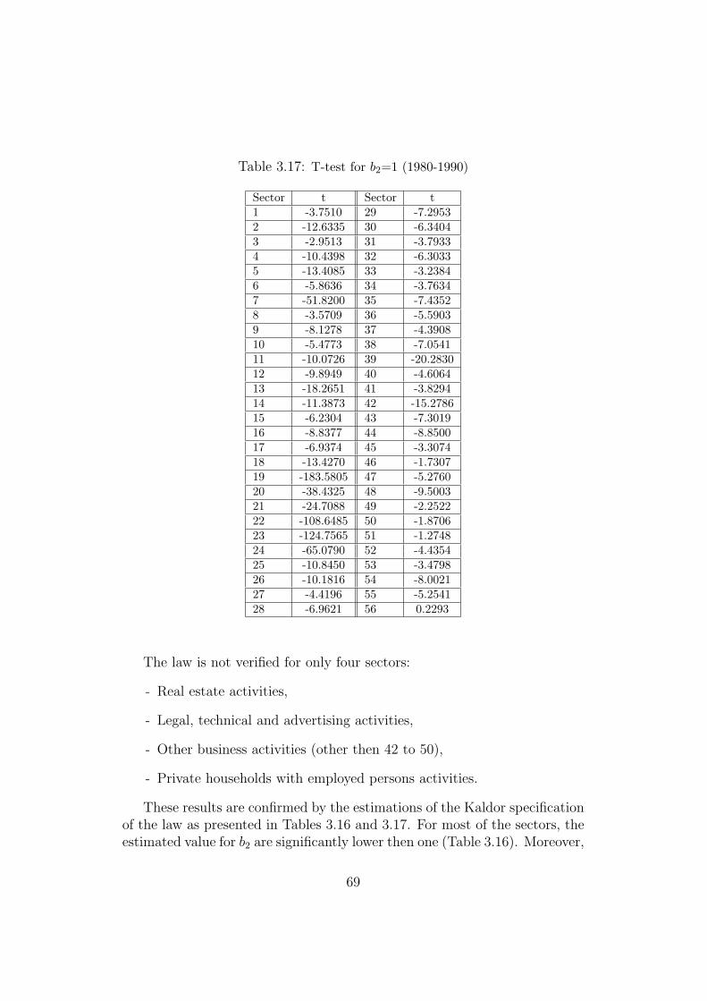
Table 3.17: T-test for b2=1 (1980-1990)
Sector t Sector t1 -3.7510 29 -7.29532 -12.6335 30 -6.34043 -2.9513 31 -3.79334 -10.4398 32 -6.30335 -13.4085 33 -3.23846 -5.8636 34 -3.76347 -51.8200 35 -7.43528 -3.5709 36 -5.59039 -8.1278 37 -4.390810 -5.4773 38 -7.054111 -10.0726 39 -20.283012 -9.8949 40 -4.606413 -18.2651 41 -3.829414 -11.3873 42 -15.278615 -6.2304 43 -7.301916 -8.8377 44 -8.850017 -6.9374 45 -3.307418 -13.4270 46 -1.730719 -183.5805 47 -5.276020 -38.4325 48 -9.500321 -24.7088 49 -2.252222 -108.6485 50 -1.870623 -124.7565 51 -1.274824 -65.0790 52 -4.435425 -10.8450 53 -3.479826 -10.1816 54 -8.002127 -4.4196 55 -5.254128 -6.9621 56 0.2293
The law is not verified for only four sectors:
- Real estate activities,
- Legal, technical and advertising activities,
- Other business activities (other then 42 to 50),
- Private households with employed persons activities.
These results are confirmed by the estimations of the Kaldor specificationof the law as presented in Tables 3.16 and 3.17. For most of the sectors, theestimated value for b2 are significantly lower then one (Table 3.16). Moreover,
69
for a large number of sector b2 is not significantly different from zero. Thesecorresponds to the high value estimated for the Verdoorn coefficient.
Finally for the four sectors, the estimation for the Kaldor specificationshows the following result. The estimate for b2 appears significantly posi-tive but not significantly different from one, only for the “Other businessactivities (other then 42 to 50)” and the “Private households with employedpersons activities”. In other words, the Law does not hold for these twosectors because these are characterised by constant returns to scale. For the“Real estate activities” and the “Legal, technical and advertising” sectors,the estimation of the Law exhibits simultaneously that a2 and b2 are nonsignificantly different from zero. For these sectors, no clear relationship be-tween employment, productivity and gross output seems to occur.
We then revert to a T-test to compare the estimated values of the Ver-doorn coefficient for each sector to its estimated value for the aggregate level(‘All industry’). The results of this test are detailed in Table 3.18. For mostof the sectors, the estimated Verdoorn coefficient is not significantly differentfrom the aggregate one.
However, for the following sectors the estimated value of the coefficientappears to be significantly bigger then for the aggregate:
- Forestry,
- Food, drinks and tobacco,
- Office machinery,
- Electronic valves and tubes,
- Telecom equipment,
- Radio and TV receivers.
Among these sectors, four corresponds to electronics and manufacturing di-rectly applied to the Information and communication technologies (ICTs).
The following sectors, for which the law holds, show an estimated valuefor a2 significantly lower then the aggregate one. Most of these are traditionalmanufacturing activities:
- Clothing,
- Leather and footwear,
- Insulated wire,
70
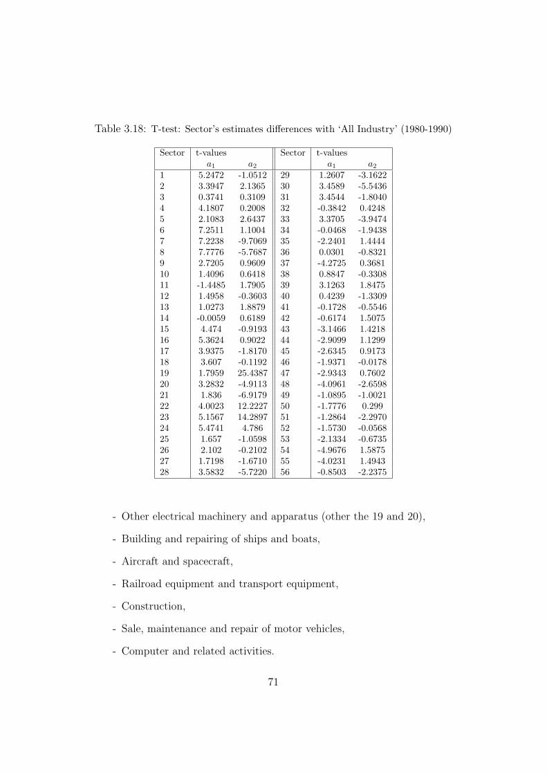
Table 3.18: T-test: Sector’s estimates differences with ‘All Industry’ (1980-1990)
Sector t-values Sector t-valuesa1 a2 a1 a2
1 5.2472 -1.0512 29 1.2607 -3.16222 3.3947 2.1365 30 3.4589 -5.54363 0.3741 0.3109 31 3.4544 -1.80404 4.1807 0.2008 32 -0.3842 0.42485 2.1083 2.6437 33 3.3705 -3.94746 7.2511 1.1004 34 -0.0468 -1.94387 7.2238 -9.7069 35 -2.2401 1.44448 7.7776 -5.7687 36 0.0301 -0.83219 2.7205 0.9609 37 -4.2725 0.368110 1.4096 0.6418 38 0.8847 -0.330811 -1.4485 1.7905 39 3.1263 1.847512 1.4958 -0.3603 40 0.4239 -1.330913 1.0273 1.8879 41 -0.1728 -0.554614 -0.0059 0.6189 42 -0.6174 1.507515 4.474 -0.9193 43 -3.1466 1.421816 5.3624 0.9022 44 -2.9099 1.129917 3.9375 -1.8170 45 -2.6345 0.917318 3.607 -0.1192 46 -1.9371 -0.017819 1.7959 25.4387 47 -2.9343 0.760220 3.2832 -4.9113 48 -4.0961 -2.659821 1.836 -6.9179 49 -1.0895 -1.002122 4.0023 12.2227 50 -1.7776 0.29923 5.1567 14.2897 51 -1.2864 -2.297024 5.4741 4.786 52 -1.5730 -0.056825 1.657 -1.0598 53 -2.1334 -0.673526 2.102 -0.2102 54 -4.9676 1.587527 1.7198 -1.6710 55 -4.0231 1.494328 3.5832 -5.7220 56 -0.8503 -2.2375
- Other electrical machinery and apparatus (other the 19 and 20),
- Building and repairing of ships and boats,
- Aircraft and spacecraft,
- Railroad equipment and transport equipment,
- Construction,
- Sale, maintenance and repair of motor vehicles,
- Computer and related activities.
71
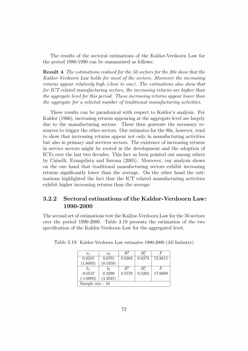
The results of the sectoral estimations of the Kaldor-Verdoorn Law forthe period 1980-1990 can be summarised as follows:
Result 4 The estimations realised for the 56 sectors for the 80s show that theKaldor-Verdoorn Law holds for most of the sectors. Moreover the increasingreturns appear relatively high (close to one). The estimations also show thatfor ICT related manufacturing sectors, the increasing returns are higher thanthe aggregate level for this period. These increasing returns appear lower thanthe aggregate for a selected number of traditional manufacturing activities.
These results can be paradoxical with respect to Kaldor’s analysis. ForKaldor (1966), increasing returns appearing at the aggregate level are largelydue to the manufacturing sectors. These then generate the necessary re-sources to trigger the other sectors. Our estimates for the 80s, however, tendto show that increasing returns appear not only in manufacturing activitiesbut also in primary and services sectors. The existence of increasing returnsin service sectors might be rooted in the development and the adoption ofICTs over the last two decades. This fact as been pointed out among othersby Cainelli, Evangelista and Savona (2005). Moreover, our analysis showson the one hand that traditional manufacturing sectors exhibit increasingreturns significantly lower than the average. On the other hand the esti-mations highlighted the fact that the ICT related manufacturing activitiesexhibit higher increasing returns than the average.
3.2.2 Sectoral estimations of the Kaldor-Verdoorn Law:1990-2000
The second set of estimations test the Kaldor-Verdoorn Law for the 56 sectorsover the period 1990-2000. Table 3.19 presents the estimation of the twospecification of the Kaldor-Verdoorn Law for the aggregated level.
Table 3.19: Kaldor-Verdoorn Law estimates 1990-2000 (All Industry)
a1 a2 R2 R2c F
0.0210 0.6701 0.8388 0.8273 72.8615(1.6093) (8.5359)
b1 b2 R2 R2c F
-0.0547 0.3299 0.5578 0.5262 17.6609(-1.6093) (4.2025)Sample size : 16
72
The estimations show that the law holds. As the estimated value forthe Verdoorn coefficient, equal to 0.6701 appears significantly different fromzero. This estimated value is significantly lower then the one found for the80s. The R2, around 0.84, is on the other side higher than the one found forthe 80s. The explanatory power of the law increased. The estimated valueof b2 is significantly lower than one, confirming the first result.
We then estimate the Verdoorn specification of the law for each of the56 sectors. These are detailed in Table 3.20. As for the previous period, theestimates for 1990-2000 show that for a large number of sectors, 46 out of56 sectors, the Kaldor-Verdoorn Law seems verified. For these 46 sectors,the estimated value of the Verdoorn coefficient appears significantly differ-ent from zero. The nature of these 46 sectors is heterogeneous, and countsprimary, manufacturing as well as service activities. The existence of increas-ing returns is, thus, not limited to the manufacturing sectors. These sectorswhere the law holds, also show a regain in the robustness of the law. Forthese sectors the value of the R2 are generally higher than for the 80s.
Among the sectors where the Kaldor-Verdoorn Law is not verified, wecount the same four services activities already pointed out in the estimatesfor the 80s, namely:
- Real estate activities,
- Legal, technical and advertising activities,
- Other business activities (other then 42 to 50),
- Private households with employed persons activities.
For three other service sectors, the estimates appears non-significant for the90s while it was in the 80s:
- Retail trade and repair of personal and households goods (except ofmotor vehicles),
- Hotels and catering,
- Computer and related activities.
73

Tab
le3.
20:
Sect
oral
esti
mat
ions
ofth
eV
erdo
orn
spec
ifica
tion
(199
0-20
00)
Sect
.a1
a2
R2
R2 c
FSe
ct.
a1
a2
R2
R2 c
F1
0.28
42(8
.131
9)0.
8906
(9.0
770)
0.85
480.
8444
82.3
924
29-0
.068
1(-
0.24
14)
0.46
42(1
.512
7)0.
1497
0.08
432.
2881
20.
2516
(4.1
785)
0.94
53(3
0.85
46)
0.98
550.
9845
952.
008
300.
1448
(1.0
832)
0.72
11(7
.114
5)0.
7833
0.76
7950
.615
30.
1887
(3.8
328)
1.02
72(4
.614
2)0.
6033
0.57
5021
.291
231
0.11
06(3
.663
3)0.
7407
(13.
9275
)0.
9327
0.92
7919
3.97
54
0.34
02(6
.673
9)0.
7899
(9.4
782)
0.86
520.
8555
89.8
359
320.
1699
(2.1
946)
1.01
86(5
.417
0)0.
6770
0.65
3929
.343
65
0.06
52(2
.301
1)1.
1916
(7.5
265)
0.80
180.
7877
56.6
488
330.
0242
(0.7
499)
0.45
49(6
.497
0)0.
7509
0.73
3142
.211
06
0.30
36(1
0.84
26)
0.72
03(2
5.86
65)
0.97
950.
9780
669.
075
34-0
.054
3(-
1.01
48)
0.96
23(5
.333
9)0.
6702
0.64
6628
.450
87
0.37
82(6
.289
1)0.
5547
(2.9
828)
0.38
860.
3449
8.89
7035
-0.0
365
(-0.
7205
)0.
8521
(8.0
819)
0.82
350.
8109
65.3
174
80.
2814
(5.5
771)
0.37
32(2
.146
9)0.
2617
0.20
504.
6092
360.
1023
(1.5
988)
0.39
21(2
.004
8)0.
2231
0.16
764.
0193
90.
0995
(2.5
910)
0.72
67(2
5.44
10)
0.97
880.
9773
647.
243
37-0
.059
5(-
1.32
57)
0.11
59(0
.647
9)0.
0291
-0.0
402
0.41
9810
0.13
47(3
.206
7)0.
9160
(8.5
434)
0.83
910.
8276
72.9
896
380.
1164
(1.4
421)
0.75
01(5
.789
2)0.
7054
0.68
4333
.514
511
0.08
22(1
.939
0)0.
8510
(17.
5466
)0.
9565
0.95
3430
7.88
439
0.18
87(2
.364
1)0.
7561
(5.9
260)
0.71
500.
6946
35.1
174
120.
1814
(4.0
867)
1.01
05(1
00.8
555)
0.00
010.
0001
1.01
7240
-0.0
112
(-0.
1607
)0.
8675
(17.
5264
)0.
9594
0.95
6330
7.17
613
0.11
76(1
.493
5)0.
8630
(14.
4380
)0.
9371
0.93
2620
8.45
641
-0.2
027
(-2.
1403
)0.
9492
(7.6
676)
0.80
770.
7939
58.7
923
14-0
.024
8(-
0.56
81)
0.93
84(9
.694
0)0.
8703
0.86
1193
.973
842
0.13
21(1
.431
6)0.
8731
(11.
5504
)0.
9050
0.89
8213
3.41
215
0.16
19(5
.714
4)0.
6398
(5.4
941)
0.68
310.
6605
30.1
848
430.
1337
(2.1
391)
0.54
32(5
.312
6)0.
6684
0.64
4828
.223
816
0.21
60(5
.144
7)0.
9990
(6.5
714)
0.75
520.
7377
43.1
831
44-0
.047
8(-
0.73
77)
0.84
27(7
.139
8)0.
7845
0.76
9150
.976
317
0.09
79(2
.083
5)0.
5893
(4.1
624)
0.55
310.
5212
17.3
252
45-0
.203
3(-
1.31
29)
0.64
84(5
.719
7)0.
7316
0.70
9332
.715
518
0.11
05(4
.057
8)0.
6300
(5.6
948)
0.69
850.
6769
32.4
306
46-0
.175
8(-
1.20
60)
0.56
91(1
.550
0)0.
1465
0.08
552.
4026
190.
1212
(0.4
777)
0.99
71(3
90.6
071)
0.00
000.
0000
1.52
5747
-0.2
858
(-2.
2217
)0.
8411
(11.
0220
)0.
8967
0.88
9312
1.48
420
0.21
30(2
.360
4)0.
3561
(2.2
889)
0.27
230.
2203
5.23
9148
-0.0
754
(-0.
1786
)0.
1902
(0.9
608)
0.06
19-0
.005
10.
9232
210.
1643
(4.7
909)
0.57
44(6
.877
8)0.
7716
0.75
5347
.304
449
-0.1
536
(-1.
4426
)0.
8314
(28.
3171
)0.
9828
0.98
1680
1.85
622
0.00
01(0
.001
1)0.
0010
(2.5
898)
0.00
000.
0000
6.70
6850
-0.2
922
(-1.
3026
)0.
4399
(1.0
168)
0.06
880.
0022
1.03
3823
0.01
35(0
.102
7)0.
6139
(11.
3809
)0.
9088
0.90
1812
9.52
551
-0.3
087
(-1.
1856
)0.
3714
(1.0
262)
0.07
000.
0035
1.05
3024
-0.2
845
(-1.
6279
)0.
0093
(0.0
300)
0.00
01-0
.076
80.
0009
520.
0202
(0.6
161)
0.62
53(3
.194
8)0.
4216
0.38
0310
.206
625
-0.4
750
(-2.
7873
)-0
.001
4(-
0.00
34)
0.00
00-0
.071
40.
0000
53-0
.086
3(-
2.33
73)
0.80
74(8
.950
6)0.
8512
0.84
0680
.112
426
0.11
71(0
.299
0)0.
5452
(2.3
555)
0.28
380.
2327
5.54
8254
-0.1
164
(-3.
5779
)0.
7053
(10.
3518
)0.
8844
0.87
6210
7.15
927
0.10
94(1
.701
9)0.
9098
(14.
2493
)0.
9355
0.93
0920
3.04
255
-0.2
544
(-2.
7022
)1.
1674
(3.5
685)
0.47
630.
4389
12.7
344
280.
1891
(2.4
239)
0.06
78(0
.409
8)0.
0119
-0.0
587
0.16
7956
0.01
89(0
.176
4)-0
.173
2(-
0.86
58)
0.06
97-0
.023
30.
7496
74
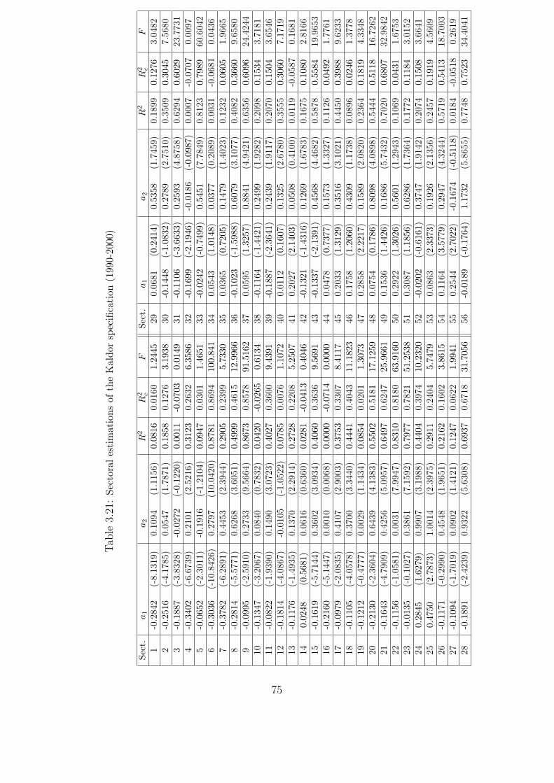
Tab
le3.
21:
Sect
oral
esti
mat
ions
ofth
eK
aldo
rsp
ecifi
cati
on(1
990-
2000
)
Sect
.a1
a2
R2
R2 c
FSe
ct.
a1
a2
R2
R2 c
F1
-0.2
842
(-8.
1319
)0.
1094
(1.1
156)
0.08
160.
0160
1.24
4529
0.06
81(0
.241
4)0.
5358
(1.7
459)
0.18
990.
1276
3.04
822
-0.2
516
(-4.
1785
)0.
0547
(1.7
871)
0.18
580.
1276
3.19
3830
-0.1
448
(-1.
0832
)0.
2789
(2.7
510)
0.35
090.
3045
7.56
803
-0.1
887
(-3.
8328
)-0
.027
2(-
0.12
20)
0.00
11-0
.070
30.
0149
31-0
.110
6(-
3.66
33)
0.25
93(4
.875
8)0.
6294
0.60
2923
.773
14
-0.3
402
(-6.
6739
)0.
2101
(2.5
216)
0.31
230.
2632
6.35
8632
-0.1
699
(-2.
1946
)-0
.018
6(-
0.09
87)
0.00
07-0
.070
70.
0097
5-0
.065
2(-
2.30
11)
-0.1
916
(-1.
2104
)0.
0947
0.03
011.
4651
33-0
.024
2(-
0.74
99)
0.54
51(7
.784
9)0.
8123
0.79
8960
.604
26
-0.3
036
(-10
.842
6)0.
2797
(10.
0420
)0.
8781
0.86
9410
0.84
134
0.05
43(1
.014
8)0.
0377
(0.2
089)
0.00
31-0
.068
10.
0436
7-0
.378
2(-
6.28
91)
0.44
53(2
.394
4)0.
2905
0.23
995.
7330
350.
0365
(0.7
205)
0.14
79(1
.402
3)0.
1232
0.06
051.
9665
8-0
.281
4(-
5.57
71)
0.62
68(3
.605
1)0.
4999
0.46
1512
.996
636
-0.1
023
(-1.
5988
)0.
6079
(3.1
077)
0.40
820.
3660
9.65
809
-0.0
995
(-2.
5910
)0.
2733
(9.5
664)
0.86
730.
8578
91.5
162
370.
0595
(1.3
257)
0.88
41(4
.942
1)0.
6356
0.60
9624
.424
410
-0.1
347
(-3.
2067
)0.
0840
(0.7
832)
0.04
20-0
.026
50.
6134
38-0
.116
4(-
1.44
21)
0.24
99(1
.928
2)0.
2098
0.15
343.
7181
11-0
.082
2(-
1.93
90)
0.14
90(3
.072
3)0.
4027
0.36
009.
4391
39-0
.188
7(-
2.36
41)
0.24
39(1
.911
7)0.
2070
0.15
043.
6546
12-0
.181
4(-
4.08
67)
-0.0
105
(-1.
0522
)0.
0785
0.00
761.
1072
400.
0112
(0.1
607)
0.13
25(2
.678
0)0.
3555
0.30
607.
1719
13-0
.117
6(-
1.49
35)
0.13
70(2
.291
4)0.
2728
0.22
085.
2507
410.
2027
(2.1
403)
0.05
08(0
.410
0)0.
0119
-0.0
587
0.16
8114
0.02
48(0
.568
1)0.
0616
(0.6
360)
0.02
81-0
.041
30.
4046
42-0
.132
1(-
1.43
16)
0.12
69(1
.678
3)0.
1675
0.10
802.
8166
15-0
.161
9(-
5.71
44)
0.36
02(3
.093
4)0.
4060
0.36
369.
5691
43-0
.133
7(-
2.13
91)
0.45
68(4
.468
2)0.
5878
0.55
8419
.965
316
-0.2
160
(-5.
1447
)0.
0010
(0.0
068)
0.00
00-0
.071
40.
0000
440.
0478
(0.7
377)
0.15
73(1
.332
7)0.
1126
0.04
921.
7761
17-0
.097
9(-
2.08
35)
0.41
07(2
.900
3)0.
3753
0.33
078.
4117
450.
2033
(1.3
129)
0.35
16(3
.102
1)0.
4450
0.39
889.
6233
18-0
.110
5(-
4.05
78)
0.37
00(3
.344
0)0.
4441
0.40
4311
.182
346
0.17
58(1
.206
0)0.
4309
(1.1
738)
0.08
960.
0246
1.37
7819
-0.1
212
(-0.
4777
)0.
0029
(1.1
434)
0.08
540.
0201
1.30
7347
0.28
58(2
.221
7)0.
1589
(2.0
820)
0.23
640.
1819
4.33
4820
-0.2
130
(-2.
3604
)0.
6439
(4.1
383)
0.55
020.
5181
17.1
259
480.
0754
(0.1
786)
0.80
98(4
.089
8)0.
5444
0.51
1816
.726
221
-0.1
643
(-4.
7909
)0.
4256
(5.0
957)
0.64
970.
6247
25.9
661
490.
1536
(1.4
426)
0.16
86(5
.743
2)0.
7020
0.68
0732
.984
222
-0.1
156
(-1.
0581
)0.
0031
(7.9
947)
0.83
100.
8180
63.9
160
500.
2922
(1.3
026)
0.56
01(1
.294
3)0.
1069
0.04
311.
6753
23-0
.013
5(-
0.10
27)
0.38
61(7
.159
2)0.
7977
0.78
2151
.253
851
0.30
87(1
.185
6)0.
6286
(1.7
364)
0.17
720.
1184
3.01
5224
0.28
45(1
.627
9)0.
9907
(3.1
988)
0.44
040.
3974
10.2
320
52-0
.020
2(-
0.61
61)
0.37
47(1
.914
2)0.
2074
0.15
083.
6641
250.
4750
(2.7
873)
1.00
14(2
.397
5)0.
2911
0.24
045.
7479
530.
0863
(2.3
373)
0.19
26(2
.135
6)0.
2457
0.19
194.
5609
26-0
.117
1(-
0.29
90)
0.45
48(1
.965
1)0.
2162
0.16
023.
8615
540.
1164
(3.5
779)
0.29
47(4
.324
4)0.
5719
0.54
1318
.700
327
-0.1
094
(-1.
7019
)0.
0902
(1.4
121)
0.12
470.
0622
1.99
4155
0.25
44(2
.702
2)-0
.167
4(-
0.51
18)
0.01
84-0
.051
80.
2619
28-0
.189
1(-
2.42
39)
0.93
22(5
.630
8)0.
6937
0.67
1831
.705
656
-0.0
189
(-0.
1764
)1.
1732
(5.8
655)
0.77
480.
7523
34.4
041
75
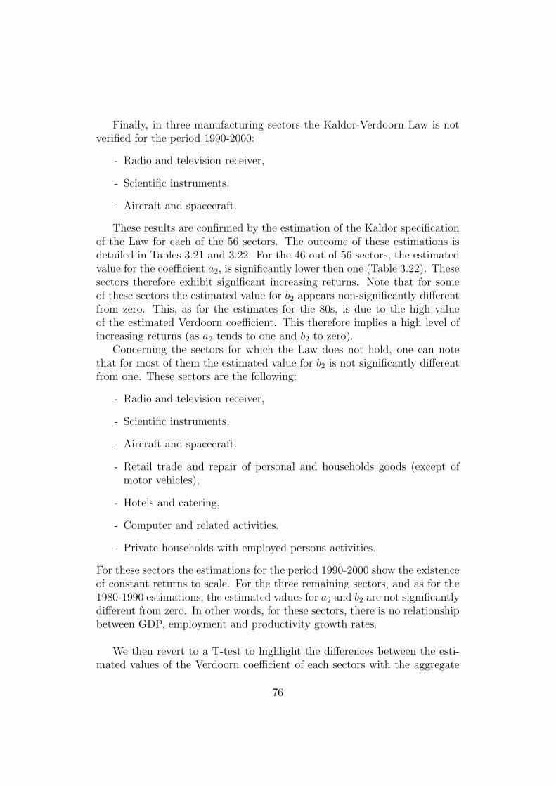
Finally, in three manufacturing sectors the Kaldor-Verdoorn Law is notverified for the period 1990-2000:
- Radio and television receiver,
- Scientific instruments,
- Aircraft and spacecraft.
These results are confirmed by the estimation of the Kaldor specificationof the Law for each of the 56 sectors. The outcome of these estimations isdetailed in Tables 3.21 and 3.22. For the 46 out of 56 sectors, the estimatedvalue for the coefficient a2, is significantly lower then one (Table 3.22). Thesesectors therefore exhibit significant increasing returns. Note that for someof these sectors the estimated value for b2 appears non-significantly differentfrom zero. This, as for the estimates for the 80s, is due to the high valueof the estimated Verdoorn coefficient. This therefore implies a high level ofincreasing returns (as a2 tends to one and b2 to zero).
Concerning the sectors for which the Law does not hold, one can notethat for most of them the estimated value for b2 is not significantly differentfrom one. These sectors are the following:
- Radio and television receiver,
- Scientific instruments,
- Aircraft and spacecraft.
- Retail trade and repair of personal and households goods (except ofmotor vehicles),
- Hotels and catering,
- Computer and related activities.
- Private households with employed persons activities.
For these sectors the estimations for the period 1990-2000 show the existenceof constant returns to scale. For the three remaining sectors, and as for the1980-1990 estimations, the estimated values for a2 and b2 are not significantlydifferent from zero. In other words, for these sectors, there is no relationshipbetween GDP, employment and productivity growth rates.
We then revert to a T-test to highlight the differences between the esti-mated values of the Verdoorn coefficient of each sectors with the aggregate
76
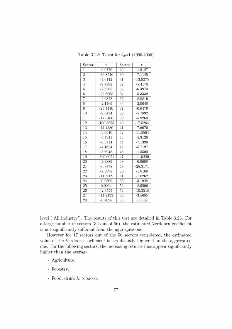
Table 3.22: T-test for b2=1 (1990-2000)
Sector t Sector t1 -9.0770 29 -1.51272 -30.8546 30 -7.11453 -4.6142 31 -13.92754 -9.4782 32 -5.41705 -7.5265 33 -6.49706 -25.8665 34 -5.33397 -2.9828 35 -8.08198 -2.1469 36 -2.00489 -25.4410 37 -0.647910 -8.5434 38 -5.789211 -17.5466 39 -5.926012 -100.8555 40 -17.526413 -14.4380 41 -7.667614 -9.6940 42 -11.550415 -5.4941 43 -5.312616 -6.5714 44 -7.139817 -4.1624 45 -5.719718 -5.6948 46 -1.550019 -390.6071 47 -11.022020 -2.2889 48 -0.960821 -6.8778 49 -28.317122 -2.5898 50 -1.016823 -11.3809 51 -1.026224 -0.0300 52 -3.194825 0.0034 53 -8.950626 -2.3555 54 -10.351827 -14.2493 55 -3.568528 -0.4098 56 0.8658
level (‘All industry’). The results of this test are detailed in Table 3.23. Fora large number of sectors (32 out of 56), the estimated Verdoorn coefficientis not significantly different from the aggregate one.
However for 17 sectors out of the 56 sectors considered, the estimatedvalue of the Verdoorn coefficient is significantly higher than the aggregatedone. For the following sectors, the increasing returns thus appear significantlyhigher than the average:
- Agriculture,
- Forestry,
- Food, drink & tobacco,
77
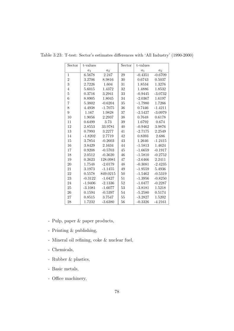
Table 3.23: T-test: Sector’s estimates differences with ‘All Industry’ (1990-2000)
Sector t-values Sector t-valuesa1 a2 a1 a2
1 6.5678 2.247 29 -0.4351 -0.67092 3.2706 8.9816 30 0.6743 0.50373 2.7226 1.604 31 1.8534 1.32764 5.6015 1.4372 32 1.4886 1.85325 0.3716 3.2941 33 -0.9445 -3.07326 8.8905 1.8045 34 -2.0367 1.61977 5.3802 -0.6204 35 -1.7980 1.72668 4.4938 -1.7075 36 0.7446 -1.42119 1.167 1.9828 37 -2.5427 -3.097910 1.9056 2.2937 38 0.7648 0.617811 0.6499 3.73 39 1.6792 0.67412 2.8553 33.9781 40 -0.9462 3.987613 0.7993 3.2277 41 -2.7175 2.254914 -1.8202 2.7719 42 0.8393 2.68615 3.7854 -0.2603 43 1.2646 -1.241516 3.8429 2.1634 44 -1.5813 1.462417 0.9208 -0.5703 45 -1.6659 -0.191718 2.0512 -0.3620 46 -1.5810 -0.275219 0.2623 128.0981 47 -2.6466 2.241120 1.7548 -2.0179 48 -0.3081 -2.423521 3.1973 -1.1455 49 -1.9559 5.493622 0.5578 849.0215 50 -1.5462 -0.531923 -0.3122 -1.0427 51 -1.3956 -0.825024 -1.9406 -2.1336 52 -1.0477 -0.228725 -3.1081 -1.6077 53 -3.8181 1.521826 0.1594 -0.5397 54 -5.2580 0.517427 0.8515 3.7547 55 -3.2827 1.520228 1.7232 -3.6380 56 -0.3326 -4.2161
- Pulp, paper & paper products,
- Printing & publishing,
- Mineral oil refining, coke & nuclear fuel,
- Chemicals,
- Rubber & plastics,
- Basic metals,
- Office machinery,
78

- Electronic valves and tubes,
- Motor vehicles,
- Air transport,
- Supporting and auxiliary transport activities, activities of travel agen-cies,
- Communications,
- Renting of machinery and equipment,
- Research and development.
The level of the increasing returns in these sectors is therefore higher thanthe average one. No clear pattern emerges, as these sectors are part of theprimary as well as manufacturing or service sectors.
For 7 of the 56 sectors, the estimated Verdoorn coefficient is significantlylower than the aggregate one for the period 1990-2000. Among these, the fol-lowing corresponds to sectors where the coefficient appeared non significantlydifferent from zero:
- Radio and television receiver,
- Hotels and catering,
- Computer and related activities.
- Real estate activities.
The remaining three sectors, show increasing returns (a2 significantlydifferent from zero and b2 significnatly different from one), but these aresignificantly lower than the average. The estimated value of the Verdoorncoefficient is significantly lower than the estimated value of these coefficientover all industries:
- Insulated wire,
- Building and repairing of ships and boats,
- Construction.
79
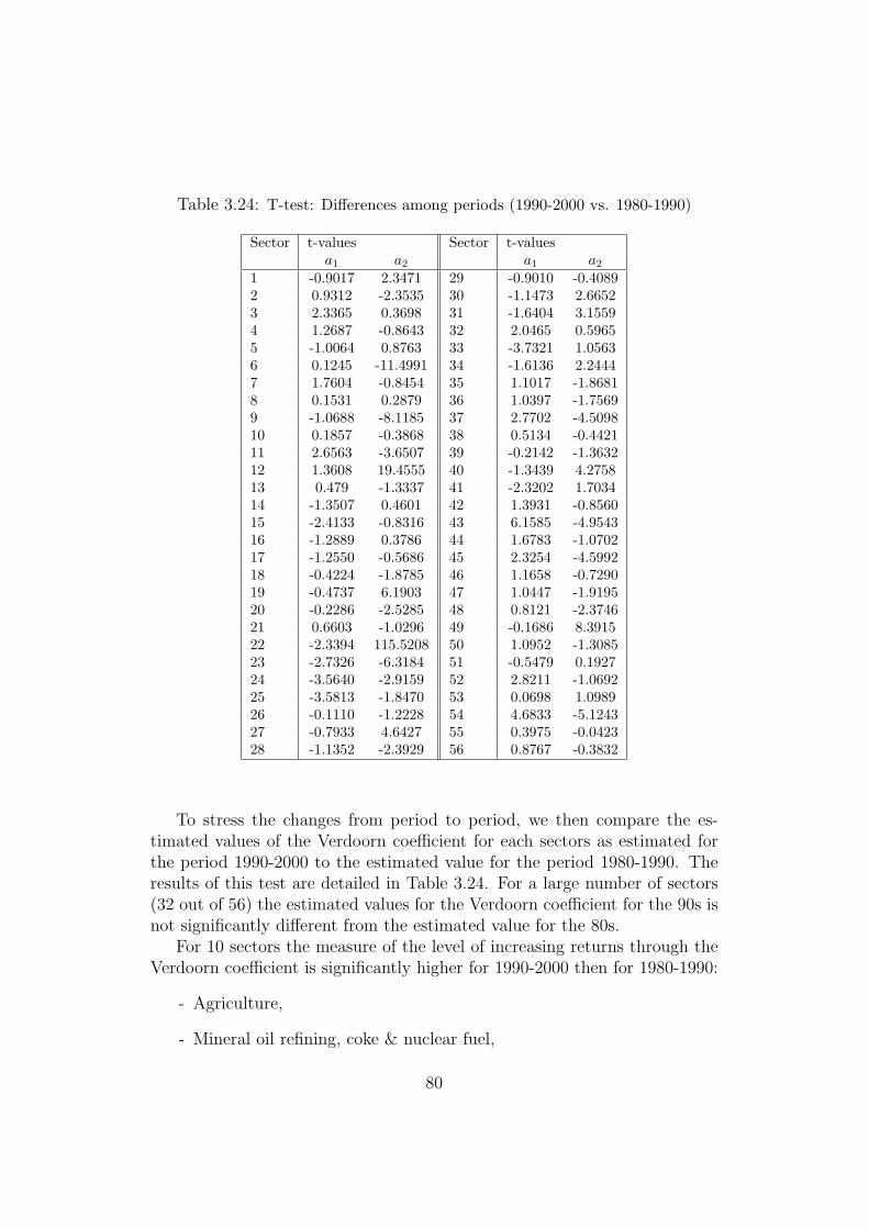
Table 3.24: T-test: Differences among periods (1990-2000 vs. 1980-1990)
Sector t-values Sector t-valuesa1 a2 a1 a2
1 -0.9017 2.3471 29 -0.9010 -0.40892 0.9312 -2.3535 30 -1.1473 2.66523 2.3365 0.3698 31 -1.6404 3.15594 1.2687 -0.8643 32 2.0465 0.59655 -1.0064 0.8763 33 -3.7321 1.05636 0.1245 -11.4991 34 -1.6136 2.24447 1.7604 -0.8454 35 1.1017 -1.86818 0.1531 0.2879 36 1.0397 -1.75699 -1.0688 -8.1185 37 2.7702 -4.509810 0.1857 -0.3868 38 0.5134 -0.442111 2.6563 -3.6507 39 -0.2142 -1.363212 1.3608 19.4555 40 -1.3439 4.275813 0.479 -1.3337 41 -2.3202 1.703414 -1.3507 0.4601 42 1.3931 -0.856015 -2.4133 -0.8316 43 6.1585 -4.954316 -1.2889 0.3786 44 1.6783 -1.070217 -1.2550 -0.5686 45 2.3254 -4.599218 -0.4224 -1.8785 46 1.1658 -0.729019 -0.4737 6.1903 47 1.0447 -1.919520 -0.2286 -2.5285 48 0.8121 -2.374621 0.6603 -1.0296 49 -0.1686 8.391522 -2.3394 115.5208 50 1.0952 -1.308523 -2.7326 -6.3184 51 -0.5479 0.192724 -3.5640 -2.9159 52 2.8211 -1.069225 -3.5813 -1.8470 53 0.0698 1.098926 -0.1110 -1.2228 54 4.6833 -5.124327 -0.7933 4.6427 55 0.3975 -0.042328 -1.1352 -2.3929 56 0.8767 -0.3832
To stress the changes from period to period, we then compare the es-timated values of the Verdoorn coefficient for each sectors as estimated forthe period 1990-2000 to the estimated value for the period 1980-1990. Theresults of this test are detailed in Table 3.24. For a large number of sectors(32 out of 56) the estimated values for the Verdoorn coefficient for the 90s isnot significantly different from the estimated value for the 80s.
For 10 sectors the measure of the level of increasing returns through theVerdoorn coefficient is significantly higher for 1990-2000 then for 1980-1990:
- Agriculture,
- Mineral oil refining, coke & nuclear fuel,
80

- Office machinery,
- Electronic valves and tubes,
- Motor vehicles,
- Railroad equipment and transport equipment,
- Furniture, miscellaneous manufacturing; recycling,
- Sale, maintenance and repair of motor vehicles and motorcycles; retailsale of automotive fuel,
- Air transport,
- Research and development.
For the remaining 14 sectors the estimated values of the Verdoorn coeffi-cient are significantly lower for 1990-2000 than for 1980-1990. Among these,for the following four sectors this difference is explained by the fact that forthe last period, the estimated value for the coefficient is not significantlydifferent from zero any more while it was for 1980-1990:
- Radio and television receivers,
- Building and repairing of ships and boats,
- Hotels & catering,
- Computer and related activities.
For the other 10, the estimated coefficient is significantly different fromzero for the two periods but significantly lower in the 90s then the 80s:
- Forestry,
- Textiles,
- Wood & products of wood and cork,
- Printing & publishing ,
- Insulated wire,
- Telecommunication equipment,
- Financial intermediation, except insurance and pension funding,
81
- Activities auxiliary to financial intermediation,
- Renting of machinery and equipment,
- Health and social work.
For all these sectors, the level of increasing returns decreased but remainedpositive.
The estimation of the Verdoorn coefficient at the aggregate level appearedsignificantly lower for 1990-2000 than for 1980-1990. However this decreasemight not necessarily be due to a general reduction of the increasing returnsamong sectors. Only 14 sectors over 56 are characterised by increasing re-turns significantly lower for the 90s then for the 80s. In other words thedecrease of the aggregate level estimates might be explained by a change inthe sectoral structure of the economies.
The results of the sectoral estimations of the Kaldor-Verdoorn Law forthe period 1990-2000 can be summarised as follows:
Result 5 The estimations show that the Kaldor-Verdoorn Law still holds forthe period 1990-2000, at the aggregate, as well as the sectoral levels. However,the aggregated estimated value of the Verdoorn coefficient has significantly de-creased. The number of sectors where the Law does not hold has increasedand concern every sector of activity (primary, manufacturing as well as ser-vices). If the aggregate value of the coefficient has significantly decreased fromthe 80s to the 90s, only a minority of sectors show the same trend (14 over56).
If the Kaldor-Verdoorn Law holds at the aggregate level as well as formost of the sectors, the estimates for the period 1990-2000 reveal a higherdegree of heterogeneity then for the period 1980-1990. A larger numberof sectors do not exhibit significant increasing returns. Moreover, a largernumber of sectors’ estimations are significantly different from the aggregatedestimations. Simultaneously, the estimates show a higher degree of robust-ness for the 90s than it exhibited in the 80s. Hence, these observations leadto the conclusion that the level of increasing returns tends to become moredispersed during the 90s but more robust.
The decrease in the estimated value of the Verdoorn coefficient for theaggregated level, does not correspond to a general trend at the sectoral level.Hence most of the sectors do not exhibit significant changes in the value ofthis coefficient. In this sense, the aggregated changes seems only due to fewsectors. The aggregate result might be explained by the relative importanceof a small number of sectors. In other words both the macro and mesostructure and their changes matter to understand productivity dynamics atan aggregated level.
82
3.3 Conclusion: Towards a ‘Kaldor-Verdoorn’
Paradox ?
We aim in this chapter to answer the following question: Does the Kaldor-Verdoorn Law still mean something ? Kaldor (1966) referring to Verdoorn(1949) stressed the existence of increasing returns at the macro-economiclevel estimating first a linear relationship between the growth rate of labourproductivity and the GDP growth rate and second a linear relationship be-tween the growth rate of employment and the growth rate of GDP. Theseestimates turned out to be significant and robust. For Kaldor (1966) this ev-idence showed that capitalists economies were exhibiting increasing returns.These increasing returns constitute one of the key factor for growth, in linewith most of the modern growth theories.
These relationships known as the Kaldor-Verdoorn Law constitute a sim-ple formal measure for investigating the existence of increasing returns. How-ever, the reliability of the Law has been put into question, first due to itsstrong sensitiveness to the choice of the sample, as stressed by Rowthorn(1975). Second, from the 1980s on, Boyer and Petit (1981,1991) among oth-ers, questioned the persistence of the law. However they imputed this evi-dence to the structural change that occurred in the most advanced economiessince 1970, contrary to Rowthorn (1975) who focused on technical reasons.For these authors, the shift towards service activities, the crisis in manufac-turing activities, as well as changes in demand regimes and the increasingof the R&D based technical change replacing the capital embodied technicalchange questioned the persistence of the Law. Kaldor (1966, 1972, 1981)himself claimed that increasing returns are the characteristic of large scalemanufacturing activities.
We first estimate the law at the aggregate level for various periods intime, using different samples of countries. The results of these estimationsshow the following. First when the sample is restricted to the sample ofcountries used by Kaldor (1966), the law does not hold any more after 1970.This result can be seen as in continuity with the results found by Boyer andPetit (1981) for the 1970s. This might therefore support the argument putforward by Boyer and Petit, that the changes in both production and demandstructures led to the disappearing of increasing returns as described by theKaldor-Verdoorn Law. However when we extend the sample to the entirepre-1974 OECD member countries, the results drastically modifies. The lawis verified after 1980. Two possible explanations can be found to this result.The first, technical, is the argument put forward by Rowthorn (1975), there
83
could be outliers that biases the results. The second is linked to the divisionof labour and structural change occurring in the most advanced economiesand which have affected the peripheral ones. These structural changes arecombined with changes in the specialisation patterns. Increasing returns be-ing dependent on the structure of the economies, we can infer that thesechanges explain that the sources of increasing returns are from 1970 onwardsrather found in the peripheral countries. The understanding of aggregateproductivity dynamics is therefore highly linked to the understanding of themacro-frame and its changes.
We then estimate the Kaldor-Verdoorn Law at the sectoral level for thetwo last decades. These estimations show that for the two periods and themajority of sectors, including the non-manufacturing sectors, the law holdssignificantly. The empirical results, moreover, show a tendency towards ahigher heterogeneity in the levels and significance of the estimated parametersof the law for the last period. This heterogeneity is however not linked tothe traditional distinction between manufacturing and non-manufacturingsectors as considered by Kaldor (1966). This might put into question thearguments put forward by Boyer and Petit (1981, 1991).
The estimations also put forward another change occurring between thetwo periods: The estimated values of the parameters of the law, and there-fore the level of increasing returns, decreased significantly. This decrease isnot linked to a general trend in the estimates at the sectoral level but ratherlinked to changes in a limited number of sectors. This again stresses theimportance of the macro-frame and its changes in understanding the aggre-gated productivity dynamics.
The results of these two sets of estimations might be somehow paradoxi-cal. The arguments put forward in explaining the different results occurringat the macro-level, based on Boyer and Petit (1981, 1991), relied on structuralchange and de-industrialisation of the most advanced economies and the mi-gration of these activities towards peripheral economies. However, sectoralestimates showed that not only manufacturing activities exhibit increasingreturns during the 80s and the 90s, but most of the considered sectors. De-industrialisation does not then seem to provide a clear explanation for theseempirical facts. The tendency towards more heterogeneous values of theincreasing returns shows that the differences among sector’s endowments inincreasing returns do not rely anymore on the traditional distinction betweenprimary, secondary and tertiary activity, as stressed by Kaldor (1966), buton a more subtle distinction. This requires future investigations, particularlyon the micro-determinants of these increasing returns.
84
Chapter 4
Evolutionary ModellingTechnological Dynamics AndThe Kaldor-Verdoorn Law
As illustrated by the previous chapters, the Kaldor-Verdoorn Law proposesa simple alternative for the empirical identification of the existence of in-creasing returns at the aggregated level. The use of the Kaldor-VerdoornnLaw, because of its aggregated form, allows to avoid the “abuse” of micro-level assumptions, either on the functional form of an aggregate productionfunction, or on the behaviours of economic agents. The empirical validationof the law, as shown in the previous chapters is limited to the identificationand quantification of the increasing returns.
The Kaldor-Verdoorn Law itself does not provide any explanation onthe mechanisms underlying technical change seems. According to Kaldor(1966), however, the increasing returns are of a twofold type: Static increas-ing returns corresponds to the traditional increasing returns to scale usuallyattributed to labour specialisation and/or learning-by-doing. Dynamic in-creasing returns are attributed to gains in efficiency due to the replacementof the production capacities through investments. These foundations broughtto the Kaldor-Verdoorn Law by Kaldor remained verbal. The Schumpete-rian/Evolutionary approach could, as discussed in Chapter 2, potentiallyprovide a formal micro-foundation to the Kaldor-Verdoorn Law. They rootthe existence of increasing returns in the micro-dynamics resulting from theemergence and diffusion of technologies.
We develop, in this chapter, a simple micro-founded model of techni-cal change in-line with the evolutionary literature. We use the model totest, first, the presence of a Kaldor-Verdoorn Law as a property of the mi-
85
cro dynamics. Second, we bring into light the effect of some key micro-characteristics of the model on the estimates of the Kaldor-Verdoorn Law.
The chapter is organised as follows: Next section describes the micro-founded model, and the following one provides the results from numericalsimulations.
4.1 An Evolutionary model of technical change
and firm dynamics
As discussed in Chapter 2, the evolutionary analysis of technical changeproposes a formal representation of Schumpeter’s thought. Technical change,as a key factor for economic dynamics, emerges unevenly and unpredictably.It then diffuses across the economies, disrupting the established economicequilibrium. Technical change is therefore an out-of-equilibrium process.
The evolutionary interpretation of Schumpeter’s analysis relies on analo-gies with the formalisation to be found in evolutionary biology. An economicsystem is assumed to be composed by one (or more) population of agents.These latter are defined by a set of characteristics, subject to mutations.These mutations emerge unevenly and unpredictably among the agents, gen-erating and sustaining heterogeneity in the population’s characteristics. Theagents composing the population(s) are subject to selection mechanisms. Theselection mechanism defines the level of performance of the economic agentsas function of agents characteristics.
Following the traditional evolutionary modelling1 the model, we proposehere, relies on a population of firms. These firms play two distinct butcomplementary roles in our model. They first generate technological shocksin the system, developing and using new technologies. We choose here todistinguish two phases of this process :
- Exploration or R&D. Firms first search for new production facilities,through innovation or adaptation of existing production facilities. Theoutcome of the R&D process is uncertain, and defines efficiency (interms of productivity) of the new generation of capital goods.
- Exploitation of R&D outcome. This second stage requires that firmsinvest to incorporate the outcome of research in the production process.This second stage is funded by profits, and then directly dependent onthe success of previous investments.
1See Kwasnicki (2001) for a comprehensive survey of evolutionary models of industrialdynamics, Silverberg and Verspagen (1995) for a comprehensive survey of evolutionarygrowth models.
86
The first phase aims to tackle the uneven and unpredictable nature of tech-nological shocks. The second phase, being dependent on past performancesdetermines the cumulative or path dependant nature of technical change.
The second role played by firms is to favour the diffusion of technolo-gies into the economic system. The selection mechanisms sorts out the bestperforming firms, which act as a channel for the diffusion of the most effi-cient technologies. The firms as considered in the model are assumed to bebounded rational. They are not conscious of the selection mechanisms, andtherefore do not directly try to respond to it. Firms apply simple decisionrule in terms of investment decision, pricing rule or technology adoption.The aggregate dynamics emerging from the model are then simply due tothe combination of mutation and selection dynamics into an heterogeneousand bounded rational population.
This section is organised as follows: We first characterise the agents com-posing our population, then describe the selection mechanisms, and finishwith the presentation of the mutation processes.
4.1.1 Firms characteristics: Defining the population.
Our model is structured around a population of firms indexed i, with i ∈[1; I]. In the short run (i.e. at each time step t), a given firms i is repre-sented by a production function characterised by constant returns to scale.Firms’ production process uses labour as a unique production factor. Capitalenters indirectly in the production function. The level of labour productivitydepends on the accumulated generations of capital goods. Investment in thedifferent generations of capital goods will increase labour productivity. Theproduction function will then be represented as follows :
Yi,t = Ai,t−1Li,t (4.1)
where Yi,t is the output of firm i at time t. Ai,t−1 represents labour pro-ductivity and Li,t the labour force employed in the production process. Theoutput is constrained by the demand for the firms’ products. The level ofaggregate demand (Dt) is set exogeneously. Aggregate demand is then allo-cated to each firms according to the selection process setting firms’ marketshares (zi,t). The level of production of each firm is computed as a follows:
Yi,t = zi,tDt
Labour productivity is deduced from the accumulation through time ofcapital goods. Each vintage of capital good embodies a level of labour pro-ductivity. Hence at every time step labour productivity can be expressed by
87
the following equation:
Ai,t =Ii,tai,t−1∑t
τ=1 Ii,τ
+
∑t−1τ=1 Ii,j,τ∑tτ=1 Ii,τ
Ai,t−1 (4.2)
where ai,t−1 represents the labour productivity embodied in the capital gooddeveloped by i during period t− 1. Ii,t represents the level of investment incapital goods of the firm.
Firms set prices through a mark-up process. This mark-up is applied tothe production costs (i.e. labour cost). To simplify the model, the costslinked to R&D activity are financed by profits. Thus prices can be repre-sented as follows:
pi,t = (1 + µ)w
Ai,t−1
(4.3)
where pi,t represents the price set by firm i at time t, µ the mark-up coefficientand w the nominal wage set exogeneously. It should be noted that we assumehere that the mark-up coefficients are fixed for each firms in a given economy.
The firm’s profit level will then be computed as follows:
Πi,t = pi,tYi,t − wLi,t = (1 + µ)w
Ai,t−1
Yi,t − wYi,t
Ai,t−1
Πi,t = µw
Ai,t−1
Yi,t (4.4)
In the model profits constitutes the only financial resource for firms’ invest-ments. In other words, all the decisions taken by the firms are constrainedby their profits. Their ability to capture demand shares, due to their pastperformances therefore directly affect all their decision potential.
4.1.2 Defining firms performance: The selection mech-anisms.
The selection mechanism represents, in an evolutionary system, the core of itsdynamics. It sorts the various components of a population, creating motionin the system, and allocating resources within the population. The selectionprocess is usually considered by Evolutionary economics as a metaphor forthe competition mechanisms. We choose here to use a replicator dynamics tomodel the selection mechanisms 2. The replicator dynamics is usually con-sidered as a formal representation of Fisher’s principle of natural selection.
2A comprehensive view on selection mechanisms and the replicator dynamics in evolu-tionary economics can be found in Metcalfe (1998)
88
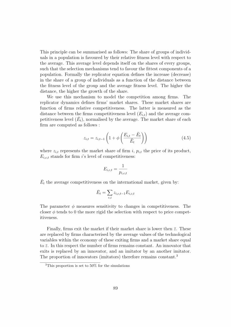
This principle can be summarised as follows: The share of groups of individ-uals in a population is favoured by their relative fitness level with respect tothe average. This average level depends itself on the shares of every groups,such that the selection mechanisms tend to favour the fittest components of apopulation. Formally the replicator equation defines the increase (decrease)in the share of a group of individuals as a function of the distance betweenthe fitness level of the group and the average fitness level. The higher thedistance, the higher the growth of the share.
We use this mechanism to model the competition among firms. Thereplicator dynamics defines firms’ market shares. These market shares arefunction of firms relative competitiveness. The latter is measured as thedistance between the firms competitiveness level (Ei,t) and the average com-petitiveness level (Et), normalised by the average. The market share of eachfirm are computed as follows :
zi,t = zi,t−1
(1 + φ
(Ei,t − Et
Et
))(4.5)
where zi,t represents the market share of firm i, pi,t the price of its product,Ei,c,t stands for firm i’s level of competitiveness:
Ei,c,t =1
pi,c,t
Et the average competitiveness on the international market, given by:
Et =∑c,i
zi,c,t−1Ei,c,t
The parameter φ measures sensitivity to changes in competitiveness. Thecloser φ tends to 0 the more rigid the selection with respect to price compet-itiveness.
Finally, firms exit the market if their market share is lower then z. Theseare replaced by firms characterised by the average values of the technologicalvariables within the economy of these exiting firms and a market share equalto z. In this respect the number of firms remains constant. An innovator thatexits is replaced by an innovator, and an imitator by an another imitator.The proportion of innovators (imitators) therefore remains constant.3
3This proportion is set to 50% for the simulations
89
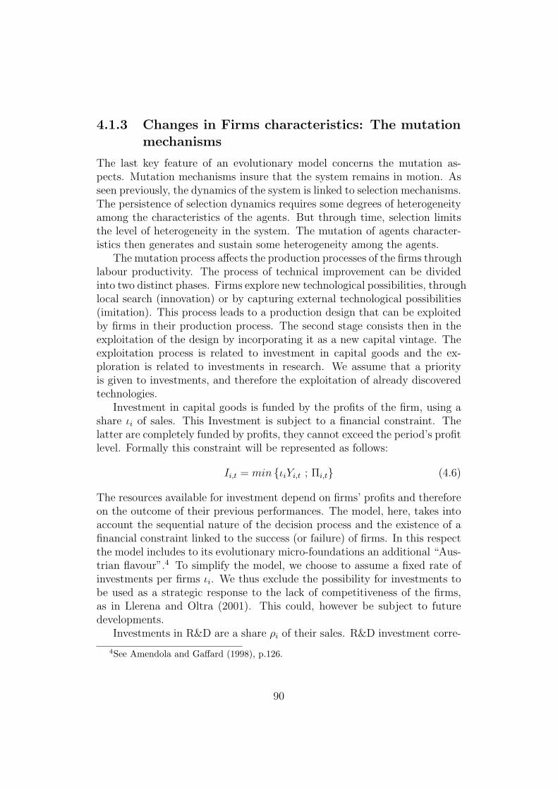
4.1.3 Changes in Firms characteristics: The mutationmechanisms
The last key feature of an evolutionary model concerns the mutation as-pects. Mutation mechanisms insure that the system remains in motion. Asseen previously, the dynamics of the system is linked to selection mechanisms.The persistence of selection dynamics requires some degrees of heterogeneityamong the characteristics of the agents. But through time, selection limitsthe level of heterogeneity in the system. The mutation of agents character-istics then generates and sustain some heterogeneity among the agents.
The mutation process affects the production processes of the firms throughlabour productivity. The process of technical improvement can be dividedinto two distinct phases. Firms explore new technological possibilities, throughlocal search (innovation) or by capturing external technological possibilities(imitation). This process leads to a production design that can be exploitedby firms in their production process. The second stage consists then in theexploitation of the design by incorporating it as a new capital vintage. Theexploitation process is related to investment in capital goods and the ex-ploration is related to investments in research. We assume that a priorityis given to investments, and therefore the exploitation of already discoveredtechnologies.
Investment in capital goods is funded by the profits of the firm, using ashare ιi of sales. This Investment is subject to a financial constraint. Thelatter are completely funded by profits, they cannot exceed the period’s profitlevel. Formally this constraint will be represented as follows:
Ii,t = min {ιiYi,t ; Πi,t} (4.6)
The resources available for investment depend on firms’ profits and thereforeon the outcome of their previous performances. The model, here, takes intoaccount the sequential nature of the decision process and the existence of afinancial constraint linked to the success (or failure) of firms. In this respectthe model includes to its evolutionary micro-foundations an additional “Aus-trian flavour”.4 To simplify the model, we choose to assume a fixed rate ofinvestments per firms ιi. We thus exclude the possibility for investments tobe used as a strategic response to the lack of competitiveness of the firms,as in Llerena and Oltra (2001). This could, however be subject to futuredevelopments.
Investments in R&D are a share ρi of their sales. R&D investment corre-
4See Amendola and Gaffard (1998), p.126.
90
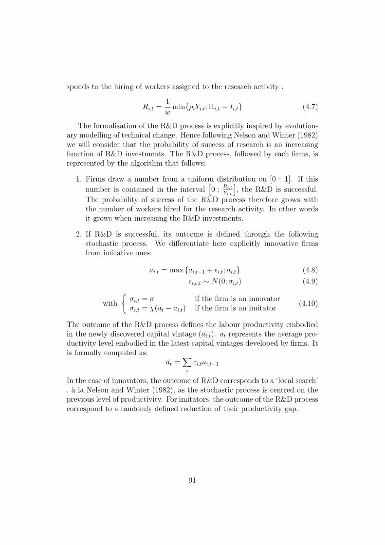
sponds to the hiring of workers assigned to the research activity :
Ri,t =1
wmin{ρiYi,t; Πi,t − Ii,t} (4.7)
The formalisation of the R&D process is explicitly inspired by evolution-ary modelling of technical change. Hence following Nelson and Winter (1982)we will consider that the probability of success of research is an increasingfunction of R&D investments. The R&D process, followed by each firms, isrepresented by the algorithm that follows:
1. Firms draw a number from a uniform distribution on [0 ; 1]. If this
number is contained in the interval[0 ; Ri,t
Yi,t
], the R&D is successful.
The probability of success of the R&D process therefore grows withthe number of workers hired for the research activity. In other wordsit grows when increasing the R&D investments.
2. If R&D is successful, its outcome is defined through the followingstochastic process. We differentiate here explicitly innovative firmsfrom imitative ones:
ai,t = max {ai,t−1 + εi,t; ai,t} (4.8)
εi,c,t ∼ N(0; σi,t) (4.9)
with
{σi,t = σ if the firm is an innovatorσi,t = χ(at − ai,t) if the firm is an imitator
(4.10)
The outcome of the R&D process defines the labour productivity embodiedin the newly discovered capital vintage (ai,t). at represents the average pro-ductivity level embodied in the latest capital vintages developed by firms. Itis formally computed as:
at =∑
i
zi,tai,t−1
In the case of innovators, the outcome of R&D corresponds to a ‘local search’, a la Nelson and Winter (1982), as the stochastic process is centred on theprevious level of productivity. For imitators, the outcome of the R&D processcorrespond to a randomly defined reduction of their productivity gap.
91
4.2 Evolutionary micro-founded technical change
and the Kaldor-Verdoorn Law: Main Sim-
ulation Results
As stated in the introduction to this chapter, we aim to show that, undersome conditions, a Kaldor-Verdoorn Law can emerge from the productivitydynamics generated by a simple evolutionary model. The model as describedassumes constant returns to scale in the short-run (i.e. for a given simulationstep). In other words we do not assume the existence of static increasing re-turns at the micro-level. If they appear, these are due to the combination ofthe two evolutionary dynamics, namely selection and mutation.
To bring this result into light, we first identify the effect of the micro-dynamics of the model on the aggregate productivity dynamics. We candecompose the micro-dynamics into three main phases:
1. The emergence of technological shocks. This phase corresponds to thearrival of new capital vintages. It occurs at the level of the innovativefirms as an outcome the R&D process.
2. The adoption of the technological shocks. This phase corresponds tothe introduction of the new capital vintages in the production process.
3. The diffusion of the shocks among the population. The diffusion phaseoccurs through two channels. First through the adoption by the imi-tating firms. Second through the selection process that allocates moreresources to the fittest firms. These have benefited from technologicalshocks and exploited them.
These phases of the micro-dynamics are directly affected by a set of param-eters. We then focus the analysis on the set of parameters described bellow:
- ιi, is defined above as the share of ressources devoted to investmentsin capital goods. We assume through the entire simulation procedurethat ρ, the share of ressources devoted to R&D equals (1 − ιi). Theparameter ιi, therefore also set the allocation of ressources betweencapital and research investments. As ιi decreases, more resources aredevoted to R&D. This favours the emergence of technological shocks.On the other side, as ιi increases, more resources are devoted to capitalinvestments. This favours the adoption of the technological shocks,translating the outcome of the shocks into productivity gains.
92
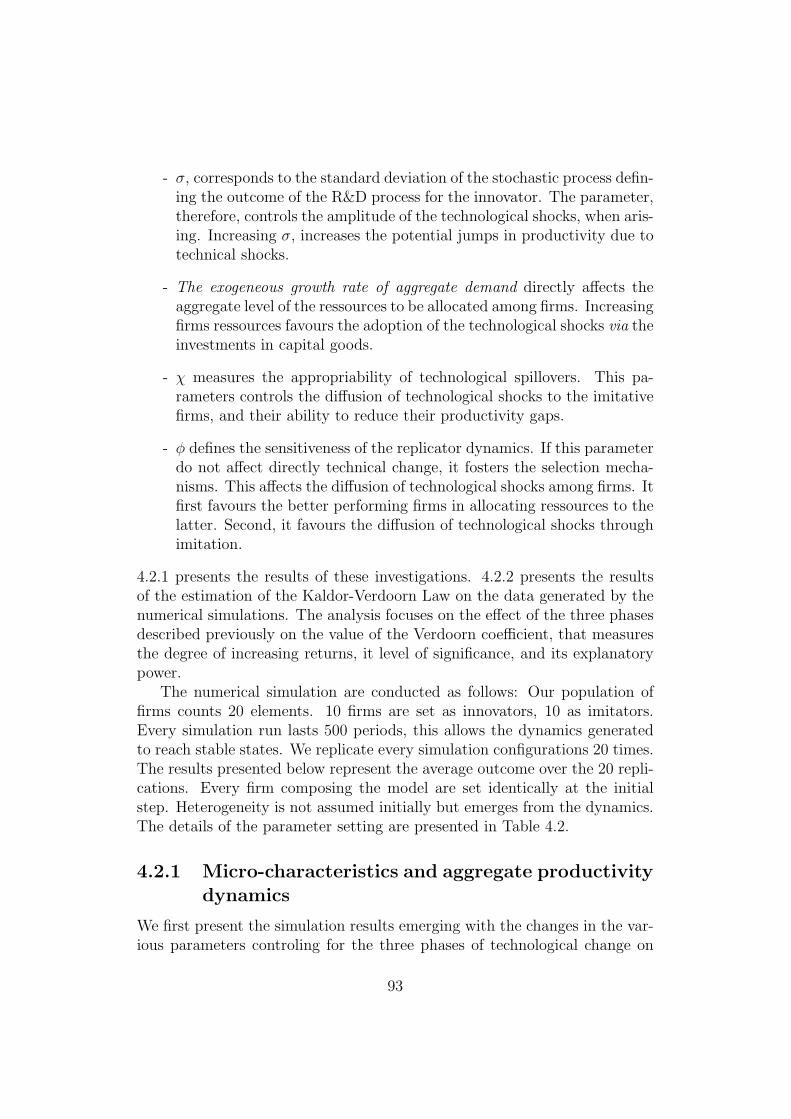
- σ, corresponds to the standard deviation of the stochastic process defin-ing the outcome of the R&D process for the innovator. The parameter,therefore, controls the amplitude of the technological shocks, when aris-ing. Increasing σ, increases the potential jumps in productivity due totechnical shocks.
- The exogeneous growth rate of aggregate demand directly affects theaggregate level of the ressources to be allocated among firms. Increasingfirms ressources favours the adoption of the technological shocks via theinvestments in capital goods.
- χ measures the appropriability of technological spillovers. This pa-rameters controls the diffusion of technological shocks to the imitativefirms, and their ability to reduce their productivity gaps.
- φ defines the sensitiveness of the replicator dynamics. If this parameterdo not affect directly technical change, it fosters the selection mecha-nisms. This affects the diffusion of technological shocks among firms. Itfirst favours the better performing firms in allocating ressources to thelatter. Second, it favours the diffusion of technological shocks throughimitation.
4.2.1 presents the results of these investigations. 4.2.2 presents the resultsof the estimation of the Kaldor-Verdoorn Law on the data generated by thenumerical simulations. The analysis focuses on the effect of the three phasesdescribed previously on the value of the Verdoorn coefficient, that measuresthe degree of increasing returns, it level of significance, and its explanatorypower.
The numerical simulation are conducted as follows: Our population offirms counts 20 elements. 10 firms are set as innovators, 10 as imitators.Every simulation run lasts 500 periods, this allows the dynamics generatedto reach stable states. We replicate every simulation configurations 20 times.The results presented below represent the average outcome over the 20 repli-cations. Every firm composing the model are set identically at the initialstep. Heterogeneity is not assumed initially but emerges from the dynamics.The details of the parameter setting are presented in Table 4.2.
4.2.1 Micro-characteristics and aggregate productivitydynamics
We first present the simulation results emerging with the changes in the var-ious parameters controling for the three phases of technological change on
93
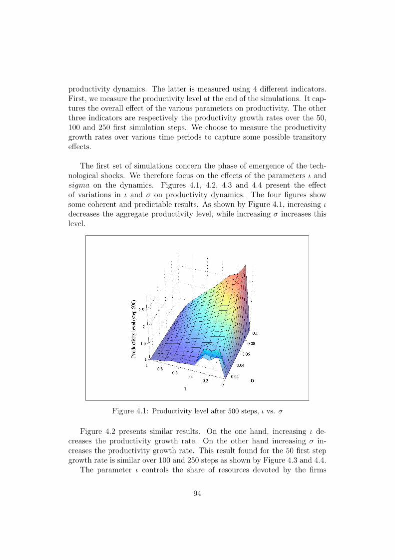
productivity dynamics. The latter is measured using 4 different indicators.First, we measure the productivity level at the end of the simulations. It cap-tures the overall effect of the various parameters on productivity. The otherthree indicators are respectively the productivity growth rates over the 50,100 and 250 first simulation steps. We choose to measure the productivitygrowth rates over various time periods to capture some possible transitoryeffects.
The first set of simulations concern the phase of emergence of the tech-nological shocks. We therefore focus on the effects of the parameters ι andsigma on the dynamics. Figures 4.1, 4.2, 4.3 and 4.4 present the effectof variations in ι and σ on productivity dynamics. The four figures showsome coherent and predictable results. As shown by Figure 4.1, increasing ιdecreases the aggregate productivity level, while increasing σ increases thislevel.
Figure 4.1: Productivity level after 500 steps, ι vs. σ
Figure 4.2 presents similar results. On the one hand, increasing ι de-creases the productivity growth rate. On the other hand increasing σ in-creases the productivity growth rate. This result found for the 50 first stepgrowth rate is similar over 100 and 250 steps as shown by Figure 4.3 and 4.4.
The parameter ι controls the share of resources devoted by the firms
94
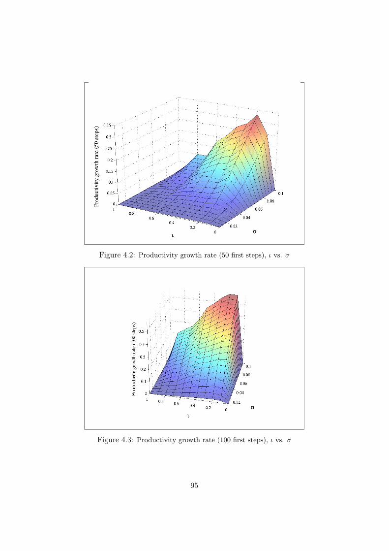
Figure 4.2: Productivity growth rate (50 first steps), ι vs. σ
Figure 4.3: Productivity growth rate (100 first steps), ι vs. σ
95
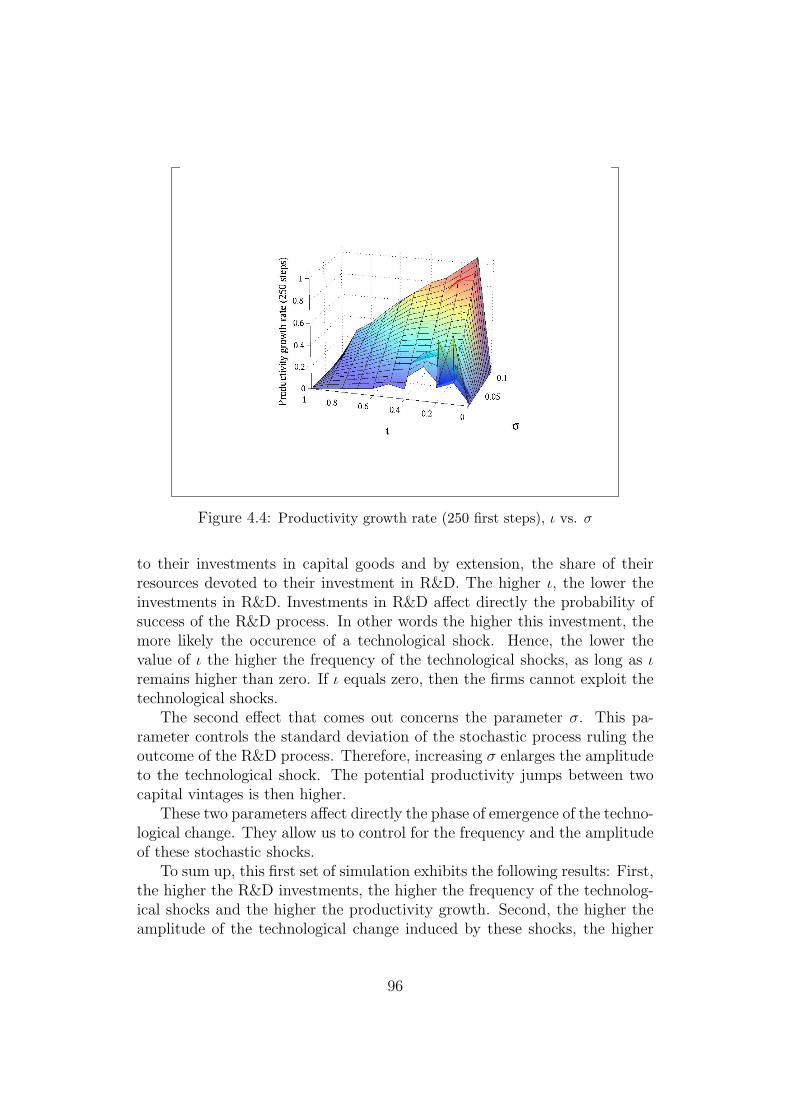
Figure 4.4: Productivity growth rate (250 first steps), ι vs. σ
to their investments in capital goods and by extension, the share of theirresources devoted to their investment in R&D. The higher ι, the lower theinvestments in R&D. Investments in R&D affect directly the probability ofsuccess of the R&D process. In other words the higher this investment, themore likely the occurence of a technological shock. Hence, the lower thevalue of ι the higher the frequency of the technological shocks, as long as ιremains higher than zero. If ι equals zero, then the firms cannot exploit thetechnological shocks.
The second effect that comes out concerns the parameter σ. This pa-rameter controls the standard deviation of the stochastic process ruling theoutcome of the R&D process. Therefore, increasing σ enlarges the amplitudeto the technological shock. The potential productivity jumps between twocapital vintages is then higher.
These two parameters affect directly the phase of emergence of the techno-logical change. They allow us to control for the frequency and the amplitudeof these stochastic shocks.
To sum up, this first set of simulation exhibits the following results: First,the higher the R&D investments, the higher the frequency of the technolog-ical shocks and the higher the productivity growth. Second, the higher theamplitude of the technological change induced by these shocks, the higher
96
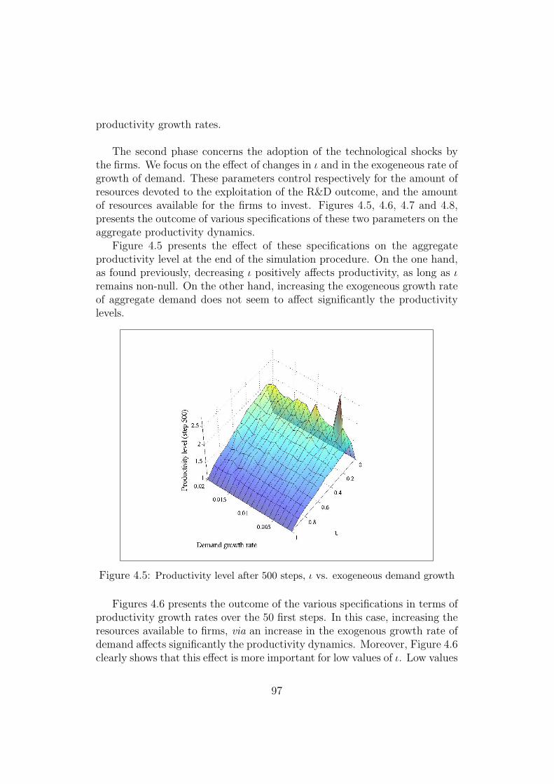
productivity growth rates.
The second phase concerns the adoption of the technological shocks bythe firms. We focus on the effect of changes in ι and in the exogeneous rate ofgrowth of demand. These parameters control respectively for the amount ofresources devoted to the exploitation of the R&D outcome, and the amountof resources available for the firms to invest. Figures 4.5, 4.6, 4.7 and 4.8,presents the outcome of various specifications of these two parameters on theaggregate productivity dynamics.
Figure 4.5 presents the effect of these specifications on the aggregateproductivity level at the end of the simulation procedure. On the one hand,as found previously, decreasing ι positively affects productivity, as long as ιremains non-null. On the other hand, increasing the exogeneous growth rateof aggregate demand does not seem to affect significantly the productivitylevels.
Figure 4.5: Productivity level after 500 steps, ι vs. exogeneous demand growth
Figures 4.6 presents the outcome of the various specifications in terms ofproductivity growth rates over the 50 first steps. In this case, increasing theresources available to firms, via an increase in the exogenous growth rate ofdemand affects significantly the productivity dynamics. Moreover, Figure 4.6clearly shows that this effect is more important for low values of ι. Low values
97
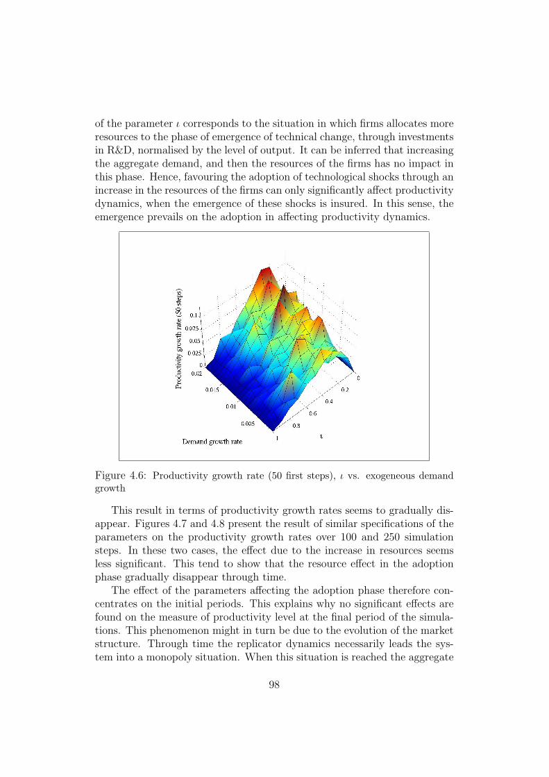
of the parameter ι corresponds to the situation in which firms allocates moreresources to the phase of emergence of technical change, through investmentsin R&D, normalised by the level of output. It can be inferred that increasingthe aggregate demand, and then the resources of the firms has no impact inthis phase. Hence, favouring the adoption of technological shocks through anincrease in the resources of the firms can only significantly affect productivitydynamics, when the emergence of these shocks is insured. In this sense, theemergence prevails on the adoption in affecting productivity dynamics.
Figure 4.6: Productivity growth rate (50 first steps), ι vs. exogeneous demandgrowth
This result in terms of productivity growth rates seems to gradually dis-appear. Figures 4.7 and 4.8 present the result of similar specifications of theparameters on the productivity growth rates over 100 and 250 simulationsteps. In these two cases, the effect due to the increase in resources seemsless significant. This tend to show that the resource effect in the adoptionphase gradually disappear through time.
The effect of the parameters affecting the adoption phase therefore con-centrates on the initial periods. This explains why no significant effects arefound on the measure of productivity level at the final period of the simula-tions. This phenomenon might in turn be due to the evolution of the marketstructure. Through time the replicator dynamics necessarily leads the sys-tem into a monopoly situation. When this situation is reached the aggregate
98
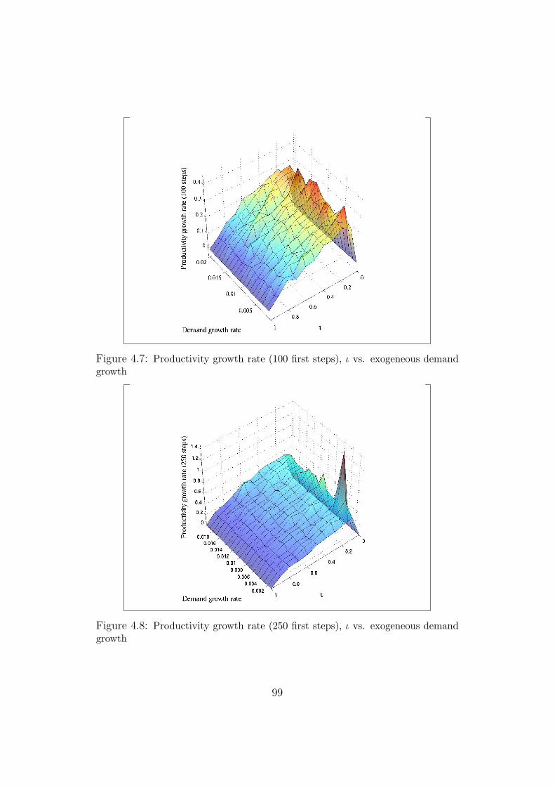
Figure 4.7: Productivity growth rate (100 first steps), ι vs. exogeneous demandgrowth
Figure 4.8: Productivity growth rate (250 first steps), ι vs. exogeneous demandgrowth
99
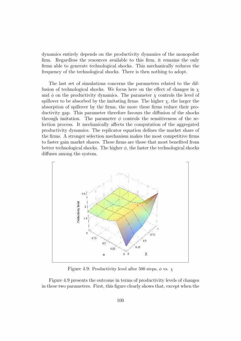
dynamics entirely depends on the productivity dynamics of the monopolistfirm. Regardless the resources available to this firm, it remains the onlyfirms able to generate technological shocks. This mechanically reduces thefrequency of the technological shocks. There is then nothing to adopt.
The last set of simulations concerns the parameters related to the dif-fusion of technological shocks. We focus here on the effect of changes in χand φ on the productivity dynamics. The parameter χ controls the level ofspillover to be absorbed by the imitating firms. The higher χ, the larger theabsorption of spillover by the firms, the more these firms reduce their pro-ductivity gap. This parameter therefore favours the diffusion of the shocksthrough imitation. The parameter φ controls the sensitiveness of the se-lection process. It mechanically affects the computation of the aggregatedproductivity dynamics. The replicator equation defines the market share ofthe firms. A stronger selection mechanism makes the most competitive firmsto faster gain market shares. These firms are those that most benefited frombetter technological shocks. The higher φ, the faster the technological shocksdiffuses among the system.
Figure 4.9: Productivity level after 500 steps, φ vs. χ
Figure 4.9 presents the outcome in terms of productivity levels of changesin these two parameters. First, this figure clearly shows that, except when the
100
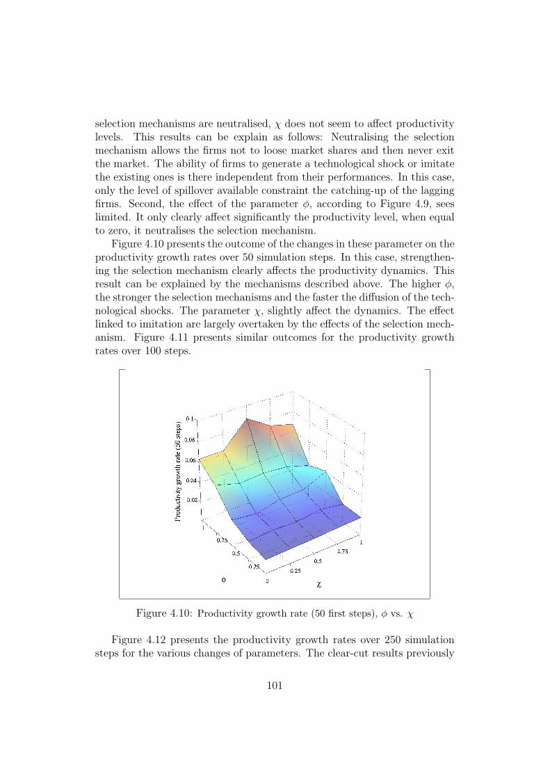
selection mechanisms are neutralised, χ does not seem to affect productivitylevels. This results can be explain as follows: Neutralising the selectionmechanism allows the firms not to loose market shares and then never exitthe market. The ability of firms to generate a technological shock or imitatethe existing ones is there independent from their performances. In this case,only the level of spillover available constraint the catching-up of the laggingfirms. Second, the effect of the parameter φ, according to Figure 4.9, seeslimited. It only clearly affect significantly the productivity level, when equalto zero, it neutralises the selection mechanism.
Figure 4.10 presents the outcome of the changes in these parameter on theproductivity growth rates over 50 simulation steps. In this case, strengthen-ing the selection mechanism clearly affects the productivity dynamics. Thisresult can be explained by the mechanisms described above. The higher φ,the stronger the selection mechanisms and the faster the diffusion of the tech-nological shocks. The parameter χ, slightly affect the dynamics. The effectlinked to imitation are largely overtaken by the effects of the selection mech-anism. Figure 4.11 presents similar outcomes for the productivity growthrates over 100 steps.
Figure 4.10: Productivity growth rate (50 first steps), φ vs. χ
Figure 4.12 presents the productivity growth rates over 250 simulationsteps for the various changes of parameters. The clear-cut results previously
101
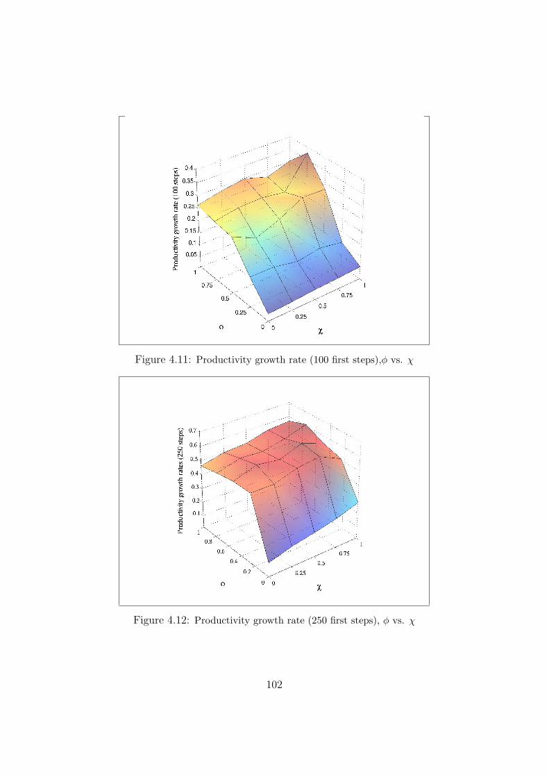
Figure 4.11: Productivity growth rate (100 first steps),φ vs. χ
Figure 4.12: Productivity growth rate (250 first steps), φ vs. χ
102
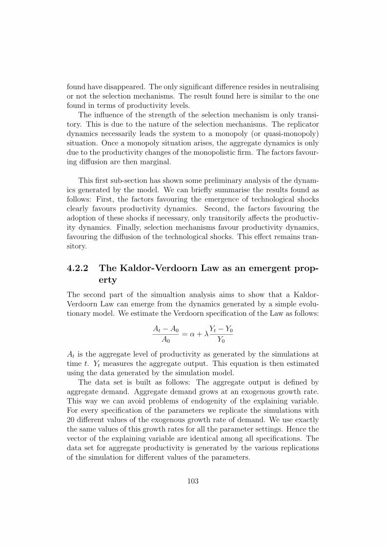
found have disappeared. The only significant difference resides in neutralisingor not the selection mechanisms. The result found here is similar to the onefound in terms of productivity levels.
The influence of the strength of the selection mechanism is only transi-tory. This is due to the nature of the selection mechanisms. The replicatordynamics necessarily leads the system to a monopoly (or quasi-monopoly)situation. Once a monopoly situation arises, the aggregate dynamics is onlydue to the productivity changes of the monopolistic firm. The factors favour-ing diffusion are then marginal.
This first sub-section has shown some preliminary analysis of the dynam-ics generated by the model. We can briefly summarise the results found asfollows: First, the factors favouring the emergence of technological shocksclearly favours productivity dynamics. Second, the factors favouring theadoption of these shocks if necessary, only transitorily affects the productiv-ity dynamics. Finally, selection mechanisms favour productivity dynamics,favouring the diffusion of the technological shocks. This effect remains tran-sitory.
4.2.2 The Kaldor-Verdoorn Law as an emergent prop-erty
The second part of the simualtion analysis aims to show that a Kaldor-Verdoorn Law can emerge from the dynamics generated by a simple evolu-tionary model. We estimate the Verdoorn specification of the Law as follows:
At − A0
A0
= α + λYt − Y0
Y0
At is the aggregate level of productivity as generated by the simulations attime t. Yt measures the aggregate output. This equation is then estimatedusing the data generated by the simulation model.
The data set is built as follows: The aggregate output is defined byaggregate demand. Aggregate demand grows at an exogenous growth rate.This way we can avoid problems of endogenity of the explaining variable.For every specification of the parameters we replicate the simulations with20 different values of the exogenous growth rate of demand. We use exactlythe same values of this growth rates for all the parameter settings. Hence thevector of the explaining variable are identical among all specifications. Thedata set for aggregate productivity is generated by the various replicationsof the simulation for different values of the parameters.
103
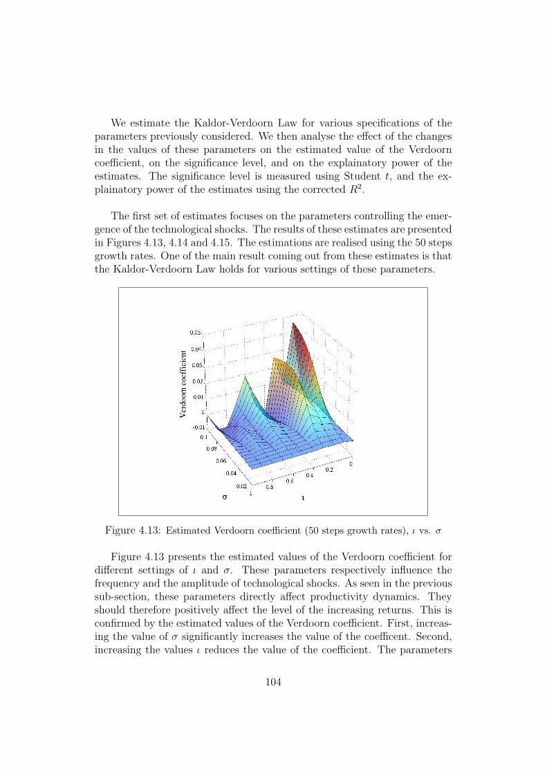
We estimate the Kaldor-Verdoorn Law for various specifications of theparameters previously considered. We then analyse the effect of the changesin the values of these parameters on the estimated value of the Verdoorncoefficient, on the significance level, and on the explainatory power of theestimates. The significance level is measured using Student t, and the ex-plainatory power of the estimates using the corrected R2.
The first set of estimates focuses on the parameters controlling the emer-gence of the technological shocks. The results of these estimates are presentedin Figures 4.13, 4.14 and 4.15. The estimations are realised using the 50 stepsgrowth rates. One of the main result coming out from these estimates is thatthe Kaldor-Verdoorn Law holds for various settings of these parameters.
Figure 4.13: Estimated Verdoorn coefficient (50 steps growth rates), ι vs. σ
Figure 4.13 presents the estimated values of the Verdoorn coefficient fordifferent settings of ι and σ. These parameters respectively influence thefrequency and the amplitude of technological shocks. As seen in the previoussub-section, these parameters directly affect productivity dynamics. Theyshould therefore positively affect the level of the increasing returns. This isconfirmed by the estimated values of the Verdoorn coefficient. First, increas-ing the value of σ significantly increases the value of the coefficent. Second,increasing the values ι reduces the value of the coefficient. The parameters
104
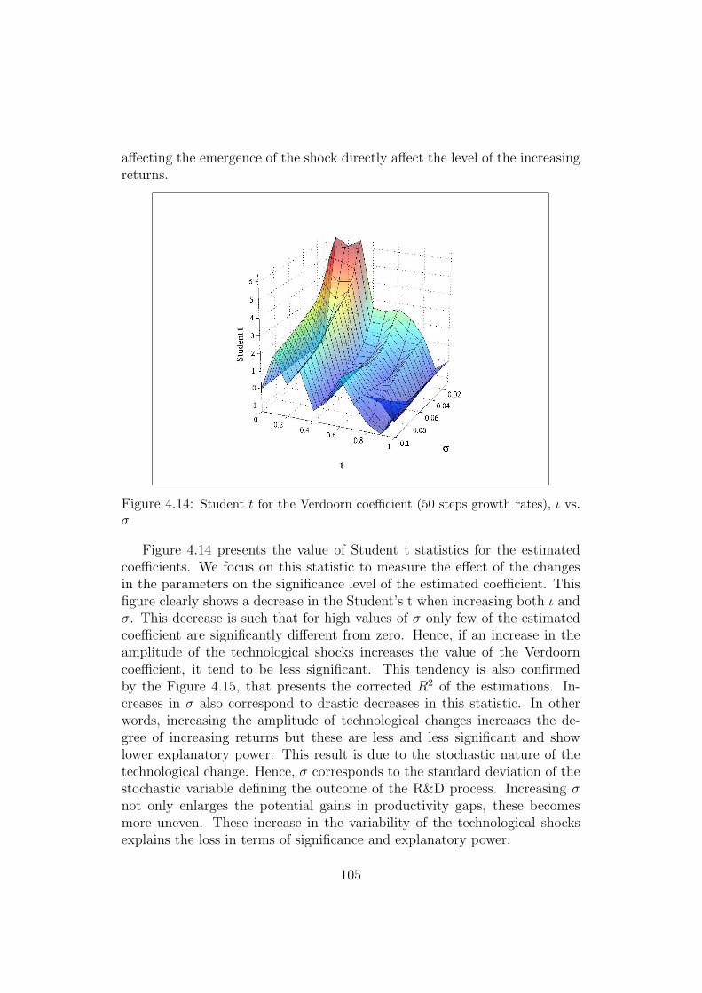
affecting the emergence of the shock directly affect the level of the increasingreturns.
Figure 4.14: Student t for the Verdoorn coefficient (50 steps growth rates), ι vs.σ
Figure 4.14 presents the value of Student t statistics for the estimatedcoefficients. We focus on this statistic to measure the effect of the changesin the parameters on the significance level of the estimated coefficient. Thisfigure clearly shows a decrease in the Student’s t when increasing both ι andσ. This decrease is such that for high values of σ only few of the estimatedcoefficient are significantly different from zero. Hence, if an increase in theamplitude of the technological shocks increases the value of the Verdoorncoefficient, it tend to be less significant. This tendency is also confirmedby the Figure 4.15, that presents the corrected R2 of the estimations. In-creases in σ also correspond to drastic decreases in this statistic. In otherwords, increasing the amplitude of technological changes increases the de-gree of increasing returns but these are less and less significant and showlower explanatory power. This result is due to the stochastic nature of thetechnological change. Hence, σ corresponds to the standard deviation of thestochastic variable defining the outcome of the R&D process. Increasing σnot only enlarges the potential gains in productivity gaps, these becomesmore uneven. These increase in the variability of the technological shocksexplains the loss in terms of significance and explanatory power.
105
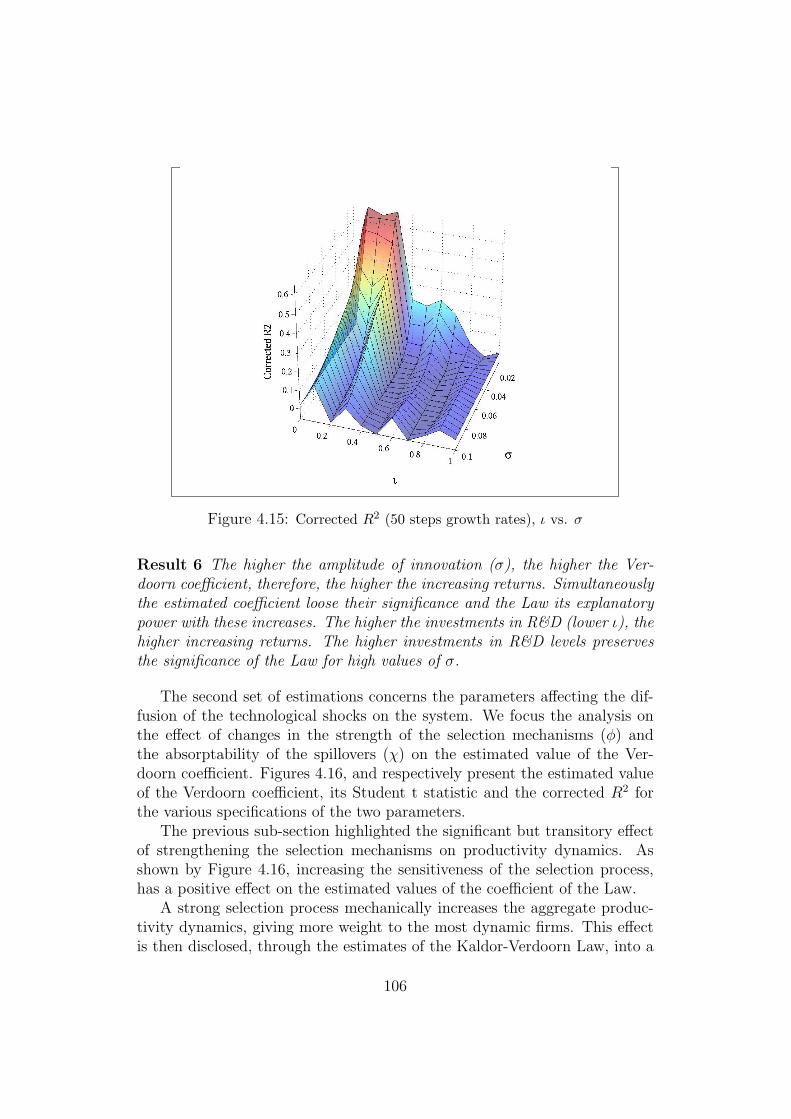
Figure 4.15: Corrected R2 (50 steps growth rates), ι vs. σ
Result 6 The higher the amplitude of innovation (σ), the higher the Ver-doorn coefficient, therefore, the higher the increasing returns. Simultaneouslythe estimated coefficient loose their significance and the Law its explanatorypower with these increases. The higher the investments in R&D (lower ι), thehigher increasing returns. The higher investments in R&D levels preservesthe significance of the Law for high values of σ.
The second set of estimations concerns the parameters affecting the dif-fusion of the technological shocks on the system. We focus the analysis onthe effect of changes in the strength of the selection mechanisms (φ) andthe absorptability of the spillovers (χ) on the estimated value of the Ver-doorn coefficient. Figures 4.16, and respectively present the estimated valueof the Verdoorn coefficient, its Student t statistic and the corrected R2 forthe various specifications of the two parameters.
The previous sub-section highlighted the significant but transitory effectof strengthening the selection mechanisms on productivity dynamics. Asshown by Figure 4.16, increasing the sensitiveness of the selection process,has a positive effect on the estimated values of the coefficient of the Law.
A strong selection process mechanically increases the aggregate produc-tivity dynamics, giving more weight to the most dynamic firms. This effectis then disclosed, through the estimates of the Kaldor-Verdoorn Law, into a
106
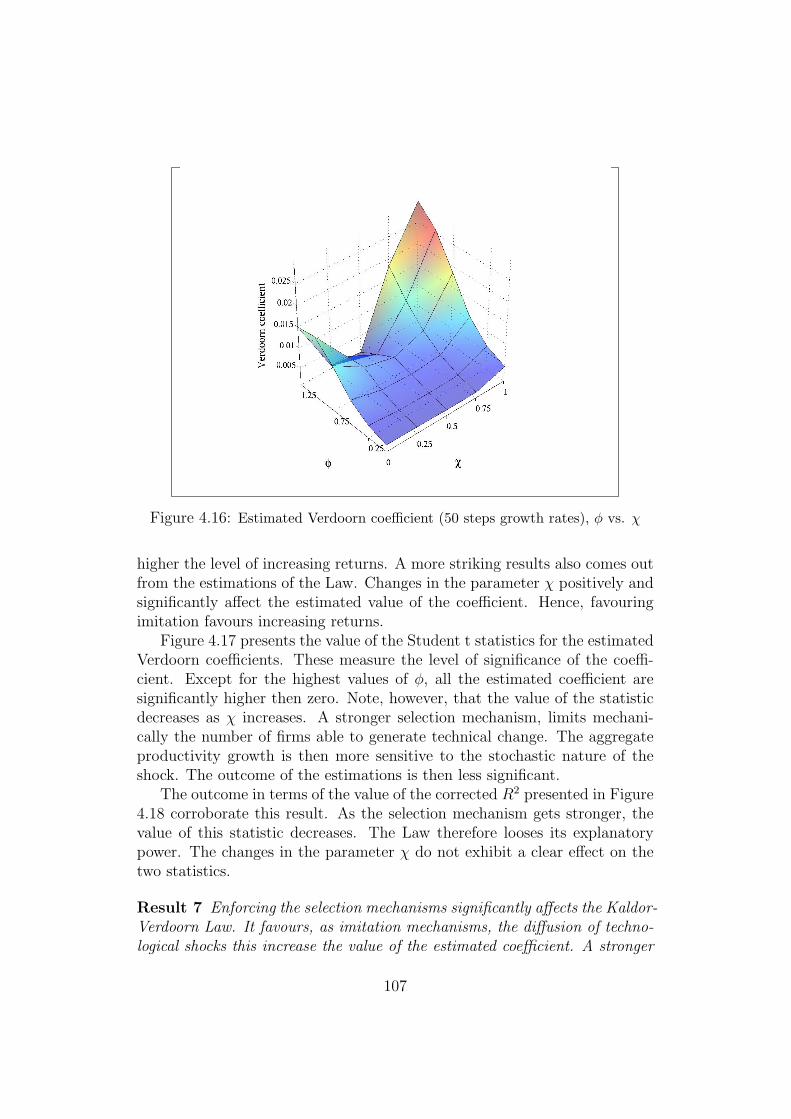
Figure 4.16: Estimated Verdoorn coefficient (50 steps growth rates), φ vs. χ
higher the level of increasing returns. A more striking results also comes outfrom the estimations of the Law. Changes in the parameter χ positively andsignificantly affect the estimated value of the coefficient. Hence, favouringimitation favours increasing returns.
Figure 4.17 presents the value of the Student t statistics for the estimatedVerdoorn coefficients. These measure the level of significance of the coeffi-cient. Except for the highest values of φ, all the estimated coefficient aresignificantly higher then zero. Note, however, that the value of the statisticdecreases as χ increases. A stronger selection mechanism, limits mechani-cally the number of firms able to generate technical change. The aggregateproductivity growth is then more sensitive to the stochastic nature of theshock. The outcome of the estimations is then less significant.
The outcome in terms of the value of the corrected R2 presented in Figure4.18 corroborate this result. As the selection mechanism gets stronger, thevalue of this statistic decreases. The Law therefore looses its explanatorypower. The changes in the parameter χ do not exhibit a clear effect on thetwo statistics.
Result 7 Enforcing the selection mechanisms significantly affects the Kaldor-Verdoorn Law. It favours, as imitation mechanisms, the diffusion of techno-logical shocks this increase the value of the estimated coefficient. A stronger
107
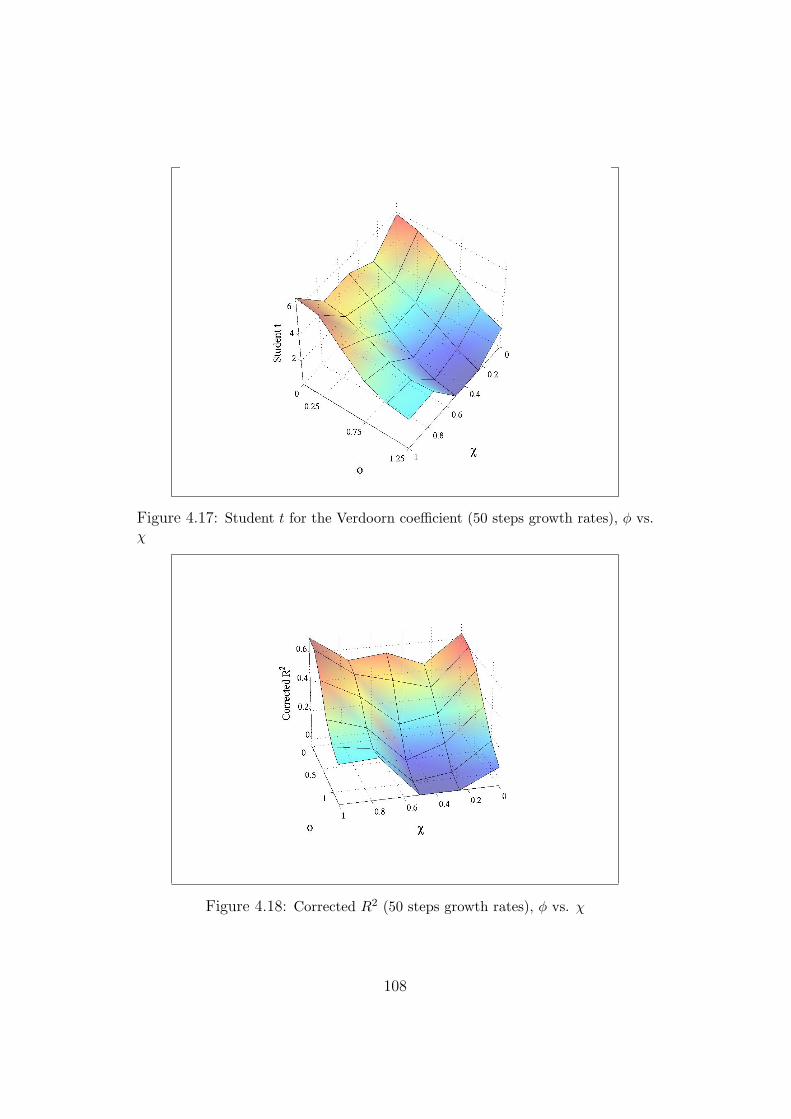
Figure 4.17: Student t for the Verdoorn coefficient (50 steps growth rates), φ vs.χ
Figure 4.18: Corrected R2 (50 steps growth rates), φ vs. χ
108
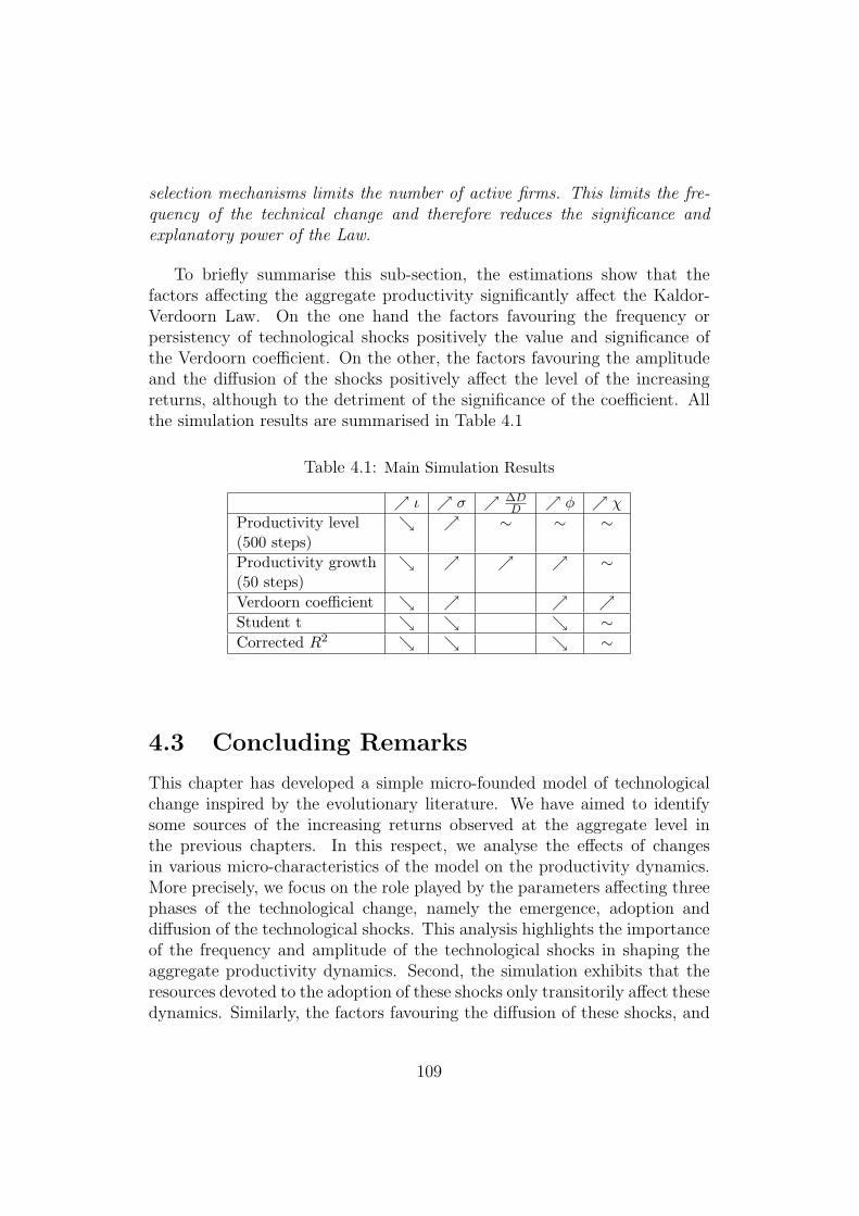
selection mechanisms limits the number of active firms. This limits the fre-quency of the technical change and therefore reduces the significance andexplanatory power of the Law.
To briefly summarise this sub-section, the estimations show that thefactors affecting the aggregate productivity significantly affect the Kaldor-Verdoorn Law. On the one hand the factors favouring the frequency orpersistency of technological shocks positively the value and significance ofthe Verdoorn coefficient. On the other, the factors favouring the amplitudeand the diffusion of the shocks positively affect the level of the increasingreturns, although to the detriment of the significance of the coefficient. Allthe simulation results are summarised in Table 4.1
Table 4.1: Main Simulation Results
↗ ι ↗ σ ↗ ∆DD ↗ φ ↗ χ
Productivity level ↘ ↗ ∼ ∼ ∼(500 steps)Productivity growth ↘ ↗ ↗ ↗ ∼(50 steps)Verdoorn coefficient ↘ ↗ ↗ ↗Student t ↘ ↘ ↘ ∼Corrected R2 ↘ ↘ ↘ ∼
4.3 Concluding Remarks
This chapter has developed a simple micro-founded model of technologicalchange inspired by the evolutionary literature. We have aimed to identifysome sources of the increasing returns observed at the aggregate level inthe previous chapters. In this respect, we analyse the effects of changesin various micro-characteristics of the model on the productivity dynamics.More precisely, we focus on the role played by the parameters affecting threephases of the technological change, namely the emergence, adoption anddiffusion of the technological shocks. This analysis highlights the importanceof the frequency and amplitude of the technological shocks in shaping theaggregate productivity dynamics. Second, the simulation exhibits that theresources devoted to the adoption of these shocks only transitorily affect thesedynamics. Similarly, the factors favouring the diffusion of these shocks, and
109
particularly, the selection mechanism, have a significant but transitory effecton productivity dynamics.
In the second part of this work, we estimated the Kaldor-Verdoorn Lawusing the data generated by the simulations for the various specificationsof the parameters. The Law is verified in most of the cases. Moreover theestimation showed that some of the micro-characteristics affect the value andsignificance level of the Verdoorn coefficient. On the one hand, increasingthe amplitude of the shocks and the strength of the selection mechanisms,increases the values but decreases the significance of the coefficient. Theselosses in significance are respectively due to increase in the unevenness of theshocks, in the first case, and a reduction of the frequency of the shocks, inthe second one. On the other hand, augmenting the resources devoted toR&D increases the frequency of the shocks, affecting positively the value andsignificance of the shocks.
The evolutionary micro-dynamics can therefore represents a possible micro-foundation of the Kaldor-Verdoorn Law. Some key parameters characterisingthese micro-dynamics have a direct influence on the values of the increasingreturns as estimated through the law. This leads us to conclude that thesources of increasing returns at the aggregate level resides in the mechanismscontrolled by these parameters, namely the frequency and amplitude of tech-nological shocks, the diffusion through imitation and the selection process.
110

Simulation Settings
Table 4.2: Parameters settings (the values by default are in italic)
ιi 0 0,1 0,2 0,3 0,4 0,5 0,6 0,7 0,8 0,9 1σ 0,01 0,015 0,02 0,025 0,03 0,035 0,04 0,045 0,05 0,055 0,06
0,065 0,07 0,075 0,08 0,085 0,09 0,095 0,1 - - -∆DD 0,001 0,002 0,003 0,004 0,005 0,006 0,007 0,008 0,009 0,01 0,011
0,012 0,013 0,0,14 0,015 0,016 0,017 0,018 0,019 0,02 - -φ 0 0,25 0,5 0,75 1 - - - - - -χ 0 0,25 0,5 0,75 1 - - - - - -µ 1 - - - - - - - - - -w 1 - - - - - - - - - -z 0,0001 - - - - - - - - - -D0 - - - - - - - - - -zi,0 0,05 - - - - - - - - - -Ai,0 1 - - - - - - - - - -ai,0 1 - - - - - - - - - -
111

112
Summary of the Results
This second part of our thesis focused on productivity dynamics, analysingthe mechanisms behind the technological or supply-side components of thegrowth process. Most of the growth theories acknowledge the role of increas-ing returns in explaining gains in labour productivity, even if those theoriesdiverge in the formal representations of these increasing returns.
The main aim of this second part is to bridge the macro-approach to in-creasing returns proposed by the cumulative causation theory to the micro-founded dynamics of increasing returns generated by the evolutionary mod-elling.
We first propose to empirically show that, despite the structural and tech-nological changes occurred since the initial estimations realised by Verdoorn(1949) and Kaldor (1966), the Kaldor-Verdoorn Law can still be verified atboth macro and sectoral levels.
We first estimated the Law at the macro-economic level using three differ-ent samples of countries: Kaldor’s (1966) sample of 12 countries, the pre-1974OECD member sample of countries, and a third sample adding to the previ-ous one a selected number of Eastern European, Latin American and SouthEast Asian countries. We used these samples to estimate the Law for fivedecades. The results from this empirical analysis are the following.
When the estimations are realised using Kaldor’s sample of countries, thelaw does not hold any more from 1970 onwards. This result is in line withBoyer and Petit (1981, 1991), bringing supporting evidences that changes inboth production and demand structures led to the disappearing of increasingreturns as described by the Kaldor-Verdoorn Law. This result is, however,clearly disproved when we extend the sample of countries used to estimatethe Law. The Law is verified from 1980 onwards when the sample used isextended to the entire pre-1974 OECD members. The law is verified after1980. The law is always verified, from 1960 onwards, when estimated usingthe sample enlarged to newly industrialised economies from Latin America,
113
South East Asian and to some Eastern European economies.This evidence can be due to two possible explanations. The first one is
related to “technical” reasons (i.e. the choice of the countries included in thesample) and in line with Rowthorn (1975) ’s claim that there could be outliersthat biases the results. The second one is linked to the division of labourand structural change occurring in the most advanced economies since 1970.These changes induced dramatic modifications in the specialisation patterns.We inferred that the sources of increasing returns from 1970 onwards arerather to be found in the peripheral countries. This might therefore explainswhy the law holds over the enlarged samples even after 1970. Further, wemight conclude as well that the understanding of aggregate productivitydynamics is therefore tightly linked to the understanding of the macro-frameand its changes.
In the last section of Chapter 3, we estimated the Kaldor-Verdoorn Lawfor 56 sectors for the two last decades. The empirical analysis showed thatfor the two periods and the most of sectors, including the non-manufacturingsectors, the law significantly holds. The empirical analysis, however, showedan increase of the heterogeneity in the levels and significance of the estimatedparameters of the law. Paradoxically, this heterogeneity does not correspondto the traditional distinction between manufacturing and non-manufacturingsectors as considered by Kaldor (1966). In some sense, this might somehowquestion the analysis presented by Boyer and Petit (1981, 1991).
Further, the results highlighted that some changes occurring in the es-timated values of the Kaldor-Verdoorn Law’s parameters at the aggregatedlevel were not linked to a general trend found among all the sectors. Thedecrease observed in the estimated value of the Verdoorn coefficient seemsrather to correspond to changes occurring in a limited number of sectors.This again stressed the importance of the macro-frame and its changes whenanalysing the aggregated productivity dynamics.
Chapter 4 has developed a simple micro-founded model of technologicalchange inspired by the evolutionary literature. We draw upon this model toidentify some sources of the increasing returns as represented by the Kaldor-Verdoorn Law. In this respect, we analyse the effects of changes in variousmicro-characteristics of the model on the estimates of the Law using the datagenerated with the simulation model. The results found can be summarisedas follows.
The Law is verified in most of the cases. The empirical evidence hasshown that some of the micro-characteristics significantly affect the value,significance and robustness of the estimates. On the one hand, increasingthe amplitude of the technological shocks and the strength of the selection
114
mechanisms makes the values to be higher, but it decreases the significance ofthe coefficient, and the robustness of the Law. These results are respectivelydue to the increase in the unevenness of the shocks, in the first case, and areduction of the frequency of the shocks, in the second one. On the otherhand, augmenting the resources devoted to R&D makes the frequency of theshocks to increase, affecting positively the value, significance and robustnessof the estimated coefficients.
The evolutionary model might then represent a plausible micro-foundationof the Kaldor-Verdoorn Law. In line with this result, we choose to introducethis micro-model to formalise the technological dynamics within the macro-models developed in the next part of this thesis.
115

116

Part III
Macro-Constraints, TechnicalChange And Growth Rates
Differences
117

118
Introduction
The aim of this third part is to propose a formal framework to investigatethe sources and nature of growth rates differences across economies. Theseinvestigations make extensive use of theoretical models.
Contrary to Verspagen (1993) that proposes a Evolutionary re-readingof a cumulative causation model, incorporating explicit selection mecha-nisms but keeping the analysis at a macro-scale, the models developed belowcontain Evolutionary micro-foundations for technical change. These microfounded dynamics are integrated to macro-frames directly in-line with cu-mulative causation models. Hence, following the Evolutionary precepts weconsider that technical change is a micro-process emerging from heteroge-neous and bounded rational firms. These firms are subject to mutations, i.e.changes in their production processes through innovation or imitation. Mu-tations are path-dependant; technical change is a function of firms’ techno-logical history as well as their past performance, due to financial constraints.Finally firms are subject to a selection mechanism, this process ought to sortthe most performing firms allocating them the highest market shares. Thisprocess is formally set at the macro-level in our frameworks.
Following the Post Keynesian approaches, the level of aggregate demanddefines the aggregated level of firms’ output. The demand dynamics there-fore constrain the firms’ production dynamics. The selection mechanismsare coupled to demand dynamics in allocation among firms. Second macro-component, wage dynamics affect directly firms’ production costs and there-fore their prices and competitiveness level. These two macro componentstherefore act on the micro-dynamics as macro-constraints. But as we seewith the formal description of our various models, these macro-constraintsthemselves are directly affected by micro-dynamics. Our model therefore in-tegrates to the evolutionary frame a set of feedback mechanisms from macro-to-micro but also from micro-to-macro. This part of our work presents threemodels illustrating the importance of these feedbacks in explaining growthrates differences across the economies.
119
Chapter 5 proposes a one-sector growth model were the macro-frameis directly inspired by the Dixon and Thirlwall (1975) or Thirlwall (1979)modelling of Kaldor’s cumulative causation. Aggregate demand dynamics isthere function of its external component through a multiplier deduced fromthe balance of payment constraint.
Chapter 6 extends the previous model introducing a multi-sectoral di-mension to the balance of payment constraint based modelling of aggregatedemand dynamics. Through this extension we aim to stress the role of sec-toral specialisation in generating growth rate differences.
Finally Chapter 7 proposes to release the balance of payment constraintand introduces in demand dynamics sectoral interdependencies of demandas well as satiation levels. Through this we aim to stress the importanceof the sectoral structure of economies as well as there changes in explain-ing growth rates differences, this also allows us to relativise some resultspreviously found.
120
Chapter 5
Balance of Payment Constraintand Growth Rate Differences
The purpose of this chapter1 is to build a simple model, integrating someof the main features discussed previously and focusing its application tothe growth rate divergence among integrated economies. It constitutes abaseline model for all the developments conducted in the coming chapters ofthis thesis.
This simple one-sector model relies on Kaldor’s cumulative causation ap-proach to growth mechanisms. The main aspect of Kaldorian approaches(Kaldor (1972, 1981) ; Dixon and Thirlwall (1975) ; Verspagen (2002)) isessentially based on two principles : First output growth is driven by thegrowth of aggregate demand, so that growth and technological progress aredemand-driven processes. In Kaldor’s mind this aggregate demand factordriving growth is concretely represented by the growth of exports that aredriven by the country’s degree of international competitiveness. FormallyGDP growth rate is deduced from the balance of payment constraint, in-cluding then all these elements. Second, productivity is a “by-product ofoutput”; this is due to the existence of dynamic increasing returns throughthe Verdoorn law and the mechanisms underlying it. The interrelation be-tween these two mechanisms, growth rates tends, through the circular andcumulative mechanisms, to be maintained or increased over time. The maindrawbacks of the approach is the “Kaldor-Verdoorn black box”. We chooseto open this box and substitute it with a micro-founded technical change,using an evolutionary model of industrial dynamics a la Nelson and Winter(1982). The main task is here to model the innovation process to endogeniesthe evolution of productivity. In other words we choose to close the model
1This chapters draws upon the model presented in Llerena and Lorentz (2004b).
121
with a micro-founded alternative to the Kaldor-Verdoorn Law, as the onedeveloped in Chapter 4.
Our model then preserves one of the major feature of the different ap-proaches it combines : unlike new growth theories, it never assumes full em-ployment, and never considers a general equilibrium framework for analysinggrowth. It means that it never assumes the existence of a natural rate ofgrowth along a given balanced growth path. The growth process is cumu-lative in this analysis because “growth creates the necessary resources forgrowth itself”2. This cumulative process allows an endogeneity of growththrough growth itself as a self-reinforcing process.
The next section is devoted to a presentation of the model, followed,in section 6.2, by the development both of the main results and of theirinterpretations.
5.1 A Growth Model with Integrated Economies:
In order to consider the co-evolution of these components, we assume that ag-gregate demand is defined at the macro-economic level, through the balanceof payment constraint. First, demand provides the necessary resources forfirms to finance their activities and development (through both R&D and in-vestments). Second, selection among firms takes place at the macro-economiclevel, as resulting from international competition. Firms located in a givencountry compete among themselves and with foreign firms on an integratedmarket3. Hence the macro-dynamics can be considered as a constraint onfirm micro-dynamics.
On the other hand technical change, a necessary engine for growth, isrooted in firms’ dynamics. The competitiveness of the entire economy relieson the firm’s ability to generate technological progress. In other words, firmscontains the essence of macro-dynamics.
As a consequence, micro and macro-dynamics are strongly interrelated.In this section we first present the macro-frame, then the micro-dynamics offirms.
The structure of the model can be described as follows: We consider a setof C economies integrated in an economic system through trade relations.An economy c ∈ [1; C], is referred to with the index c. When variables areindexed w, they concern the foreign economies with regard to the economyc.
2Leon-Ledesma (2000)3Assuming then neither trade limitations nor barriers to access foreign markets
122
Each economy counts I firms. A firm i ∈ [1; I], based in the economy cis referred to with the indexes i, c. The entire economic system then countsC economies and C ∗ I firms. The index t refers to the time step.
5.1.1 Defining the macro-economic framework:
We suppose that the economies under-consideration are part of an integratedsystem constrained by the balance of payment with fixed exchange rates ( ora common monetary system ). Moreover, we assume that the member coun-tries of the integrated system external debt with other members is restricted4.Given the monetary integration, the balance of payment adjustments throughmonetary mechanisms (exchange rates) are excluded and the balance of pay-ment constraint corresponds then to a clearing of countries trade balance.In other words imports have to match exactly exports, for each integratedeconomy.
The macro-economic framework we develop here is directly rooted in theformal interpretation of Kaldor’s cumulative causation approach of economicgrowth. These formal representations can be found among others in Dixonand Thirlwall (1975), or more recently Amable (1992), Verspagen (1993) andLeon-Ledesma (2000).
Economic growth is driven by demand. Aggregate demand is a function ofan autonomous component, represented by external demand, i.e. countries’exports. For each economy, exports are given as a function of the income ofthe rest of the world and of the market share of the economy.
Balance of payment constraint and aggregate demand:
Exports for a given economy c is given by :
Xc,t = (Yw,t)αczc,t (5.1)
where Yw,t represents the GDP of the rest of the world5, zc,t represents themarket share of the economy, on the international markets and αc income
4To simplify the model, we exclude the possibility for economies to rely on the externaldebt.
5Note that this variable is composed of the GDP level of all the other economies beingpart of this “integrated system” to which we add an exogenous component growing at agiven and fixed level. The latter represents in some sense an additive demand that comesfrom outside the “integrated system”, when running simulation we will however set theinitial value of this variable such as in level it represents a marginal share of the “rest of theworld GDP”. Note that for technical reasons we use during the simulation this variableswith a one period time lag.
123
elasticity to exports for the rest of the world.The market share of the economy is a function of the price competitiveness
of the country. In other words if the first component of the export functionrepresents the income determinant of exports, the market share then repre-sents the price component of external demand. The economy’s market shareis given by the sum of the market shares of the domestic firms (denoted zi,c,t):
zc,t =∑
i
zi,c,t
Each firm’s market share is defined through a replicator dynamics6, a functionof a firm’s relative competitiveness. Hence the market share of each firm willbe computed as follows :
zi,c,t = zi,c,t−1
(1 + φ
(Ei,c,t
Et
− 1))
(5.2)
where zi,c,t represents the market share of firm i, pi,c,t the price of its product,Ei,c,t stands for firm i’s level of competitiveness:
Ei,c,t =1
pi,c,t
Et the average competitiveness on the international market, given by:
Et =∑c,i
zi,c,t−1Ei,c,t
The parameter φ ∈ [0; 1] measures demand rigidity to price changes. Themore φ tends to 0 the more rigid demand is with respect to price competi-tiveness changes.
To complete the formal definition of the macro-economic framework, wehave to define the economy’s imports. They are basically defined followingexports’ scheme, as a function of the domestic economy income and of therest of the world’s market share. Formally imports will be represented asfollows:
Mc,t = (Yc,t)βc(1− zc,t) (5.3)
The parameter βc represents the income elasticity to import. Yc,t corre-sponds to the domestic aggregate demand, itself equal to the gross productof the economy.
6For a comprehensive view on the use of the replicator dynamics in evolutionary eco-nomics see Metcalfe (1998)
124
We assume that each economy has to satisfy the balance of paymentconstraint. In our model this corresponds to an equilibrated trade balance.An economy c’s external expenditures have to match exactly its externalresources. In terms of growth rate the balance of payment constraint canthen be represented as follows:
∆Mc,t
Mc,t−1
=∆Xc,t
Xc,t−1
(5.4)
with:
∆Xc,t
Xc,t−1
= αc∆Yw,t
Yw,t−1
+∆zc,t
zc,t−1
(5.5)
∆Mc,t
Mc,t−1
= βc∆Yc,t
Yc,t−1
− zc,t−1
1− zc,t−1
∆zc,t
zc,t−1
(5.6)
Using the balance of payment constraint we can then deduce the economies’aggregate demand growth rate as function of the rest of the world incomeand of the economy’s market share dynamics:
∆Yc,t
Yc,t−1
=αc
βc
∆Yw,t
Yw,t−1
+ec,t−1
βc
∆zc,t
zc,t−1
(5.7)
With
ec,t−1 =1
1− zc,t−1
The growth rate of market shares can be deduced from equation 5.2, wethen obtain the following expression for the GDP growth rate. With this lastrepresentation we can clearly distinguish the effect of external demand fromthe effect linked to the micro-dynamics:
∆Yc,t
Yc,t−1
=αc
βc
∆Yw,t
Yw,t−1
+ φec,t−1
βc
(Ec,t
Et
− 1)
(5.8)
The first component of the right end side of the equation captures infact Harrod’s trade multiplier. Hence GDP growth rate in our model will bedefined through the trade multiplier and through a second component linkedto the competitiveness of the economy. This second component captures themicro-dynamics, and especially the effect of technical change arising at themicro-level and influencing the directly competitiveness of the economy.
We can deduce from the expression for GDP growth rate the GDP levelat time t. It equals the domestic aggregated demand. GDP is given by:
Yc,t = Yc,t−1
[1 +
αc
βc
∆Yw,t
Yw,t−1
+ φec,t−1
βc
(Ec,t
Et
− 1)]
(5.9)
125
This expression also represents the gross production of all firms at timet. In our model, the time dimension allows aggregate supply to match en-tirely aggregate demand. We do not consider here explicitly the process ofcoordination of demand and supply in the market for goods.
Aggregate (economy wide) demand is then distributed among the firmsin the economy given their market shares on the integrated markets. It con-stitutes the first macro-economic constraint the firms have to face.
Wage dynamics:
The second macro-economic component of our model affecting firms’ dynam-ics are wages. These are set at the macro-level. Wage dynamics is correlatedto the average labour productivity growth rate of an economy as defined inthe following expression:
wc,t = wc,t−1
(1 + γ
∆Ac,t
Ac,t−1
)(5.10)
Ac,t represents the average labour productivity level of the economy c at timet.
The parameter γ ∈ [0; 1] weights the effect of labour productivity growthon wage dynamics. When γ = 1, wages are perfectly correlated with pro-ductivity growth. In this case wages gradually absorb the productivity gainseffect on firms’ competitiveness. When γ = 0, productivity growth has noimpact on wages. Its effect on competitiveness won’t be absorbed by wages.As no other variables is considered here as affecting wages, these remain fixedin this case.
The linkages between wages, productivity and competitiveness imply thatwhen γ is unitary, firms competitiveness is rather determined with respectto the firms relative productivity gains (with respect to the average). While,when γ is null, firms’ competitiveness relies on their absolute productivitygains. As we discuss later on, the wage regime has a direct impact on thetransmission of micro-level technological shocks to macro-dynamics. Wagesare not only a factor affecting firms but a major channel linking the microto the macro dimensions.
5.1.2 Evolutionary micro-foundations of technical change.
This second level of the model concerns firms and industrial dynamics. Weexplain here firms’ behaviour and characteristics. This part is largely inspiredby the model developed in Chapter 4. We assume here that each economy is
126
represented by a population of bounded rational firms. These firms mutate,by learning about the production process to improve their productivity.
Firms will have two distinct but complementary roles in our model. Firstthey produce the necessary resources to sustain economic growth, by re-sponding to the demand needs. Second they increase the competitivenessof the economy by trying to improve their productivity level to survive theselection process. This second process will be broken down into two stages:
- Exploration or R&D. Firms first search for new production facilities,through innovation or adaptation of existing production facilities. Theoutcome of the R&D process is uncertain, and defines efficiency (interms of productivity) of the new generation of capital goods.
- Exploitation of R&D outcome. This second stage requires that firmsinvest to incorporate the outcome of research in the production process.
These two stages are financed by profits, and then directly subject to thesuccess of previous investments. Formally the micro-level of the model drawslargely on the one developed in Chapter 4
Firms characteristics:
Firms’ production processes are represented by Leontiev production functionswith labour as a unique production factor. Capital enters indirectly in theproduction function by influencing labour productivity. Investment in thedifferent generations of capital goods will increase labour productivity. Theproduction function will then be represented as follows :
Yi,c,t = Ai,c,t−1Li,c,t (5.11)
where Yi,c,t is the output of firm i, producing in country c at time t. Ai,c,t−1
represents labour productivity and Li,c,t the labour force employed in theproduction process. The output is constrained by the demand directed atthe firms and defined at the macro-economic level. The level of productionof each firm is computed as a share of GDP given by their relative marketshares such as:
Yi,c,t =zi,c,t
zc,t
Yc,t
Labour productivity is a function of the firms’ accumulated generationsof capital goods through investment:
Ai,c,t =Ii,c,tai,c,t−1∑t
τ=1 Ii,c,τ
+
∑t−1τ=1 Ii,c,τ∑tτ=1 Ii,c,τ
Ai,c,t−1 (5.12)
127
where ai,c,t−1 represents the labour productivity embodied in the capital gooddeveloped by i during period t− 1. Ii,c,t represents the level of investment incapital goods of the firm. This component will be explained later. Firms setprices through a mark-up process. This mark-up is applied to the productioncosts (i.e. labour cost). To simplify the model, labour costs linked to R&Dactivity are financed by profits. Thus prices can be represented as follows:
pi,c,t = (1 + µc)wc,t−1
Ai,c,t−1
(5.13)
where pi,c,t represents the price set by firm i at time t, µc the mark-up coeffi-cient and wc,t−1 the nominal wage set at the macro level as defined above. Itshould be noted that we assume here that the mark-up coefficients are fixedfor each firms in a given economy. This insures that the share of profits inGDP is constant over time, which corresponds to one of Kaldor’s stylisedfacts.
The firm’s profit level is then be computed as follows:
Πi,c,t = pi,c,tY i, c, t− wc,t−1Li,c,t = (1 + µc)wc,t−1
Ai,c,t−1
Yi,c,t − wc,t−1Yi,c,t
Ai,c,t−1
Πi,c,t = µcwc,t−1
Ai,c,t−1
Yi,c,t (5.14)
In the model profits constitutes the only financial resource for firms’ invest-ments.
To improve their competitiveness and thus gain some market shares firmshave to improve their production processes (i.e. to increase labour pro-ductivity). The process of technical improvement can be divided into twodistinct phases. Firms explore new technological possibilities, through lo-cal search (innovation) or by capturing external technological possibilities(through spill-overs). This process leads to a production design (or capitalgood design) that can be exploited by firms in their production process. Thesecond stage consists then in the exploitation of the design by incorporatingit as a new generation of capital goods. The exploitation process is relatedto investment in capital goods and the exploration is related to investmentsin research. We assume that a priority is given to investments, and thereforethe exploitation of already discovered technologies.Investment in capital goods is financed by the profits of the firm, using ashare ιi,c of sales. Investment is subject to a financial constraint. Hence,as investments are completely financed by profits, they cannot exceed theperiod’s profit level. Formally this constraint will be represented as follows:
Ii,c,t = min {ιi,cYi,c,t ; Πi,c,t} (5.15)
128
The resources available for investment depend on firms’ profits and thereforeon the outcome of their previous performances. The model, here, takes intoaccount the sequential nature of the decision process and the existence ofa financial constraint linked to the success (or failure) of firms. In this re-spect the model includes to its evolutionary micro-foundations an additional“Austrian flavour”.7 Investments in R&D are a share ρi,c of their sales. R&Dinvestment will correspond to the hiring of workers assigned to the researchactivity :
Ri,c,t =1
wc,t−1
min{ρi,cYi,c,t; Πi,c,t − Ii,c,t} (5.16)
The formalisation of the R&D process is explicitly inspired by evolution-ary modelling of technical change. Hence following Nelson and Winter (1982)we will consider that the probability of success of research is an increasingfunction of R&D investments. Formally the R&D activity is represented bythe following procedure:
1. Firms draw a number from a uniform distribution on [0 ; 1].
2. If this number is contained in the interval[0 ; Ri,c,t
Yi,c,t
], the R&D is suc-
cessful.
3. If R&D is successful, its outcome is defined through the followingstochastic process. We differentiate here explicitly innovative firmsfrom imitative ones:
ai,c,t = max {ai,c,t−1 + εi,c,t; ai,c,t} (5.17)
εi,c,t ∼ N(0; σi,c,t) (5.18)
with
{σi,c,t = σc if the firm is an innovatorσi,c,t = χ(at − ai,c,t) if the firm is an imitator
(5.19)
The outcome of the R&D process defines the labour productivity embod-ied in the newly discovered capital vintage (ai,c,t). at represents the averageproductivity level embodied in the latest capital vintages developed by firms.It is formally computed as:
at =∑c,i
zi,c,tai,c,t−1
For innovators the R&D activity therefore resorts to ‘local searching’ as de-fined by Nelson and Winter (1982), while imitators try to reduce their tech-nological gap adopting existing technologies.
7See Amendola and Gaffard (1998), p.126)
129
Firms exit the market if their market share is lower then z. They arereplaced by firms characterised by the average values of the technologicalvariables within the economy of these exiting firms and a market share equalto z. In this respect the number of firms remains constant. An innovator thatexits is replaced by an innovator, and an imitator by an another imitator.The proportion of innovators (imitators) therefore remains constant.8
5.2 Growth Rate Difference Among Integrated
Economies : Main Simulation Results
The model as developed in the previous section aims to consider the de-terminants of possible difference in GDP growth rates among integratedeconomies. Traditionally, mainstream economics considers that the inte-gration of economies and openness to trade imply convergence due to thediffusion of knowledge and/or technologies.
For Neo-Schumpeterian evolutionary economics, growth rates differencesdepends on the balance between two effects :
- Innovation, heterogeneous among economies both in its timing and inthe outcome, that increases differences in GDP growth rates, and
- Imitation that reduces this difference.
Hence in this framework growth rate divergence directly depends on theaccessibility of technologies, innovation and imitation capabilities, and onthe decision processes linked to R&D investment.
For the Kaldorian approach growth rate difference is structural dependingon both demand and technological parameters, and cumulative, due to theemergence of vicious and virtuous circles.
As for most of the models incorporating evolutionary features we need toresort to numerical simulations9. Simulations are set through the followingscheme. We consider 5 economies, each of which counts 20 firms. All thefirms of a given economy are equally defined (same initial conditions andparameters). The details of the parameters values used can be found inTable 5.2 and 5.3.
Our analysis focuses on the determinants of growth rate differences amongthe economies composing our artificial system. The aim of the exercise is to
8This proportion is set to 50% for the simulations9We used LSD (Laboratory for Simulation Development) environment to implement
the simulations. The source code for the model can be available on request to the authors
130
highlight the existence of different and complement sources driving to specificdivergence patterns. We therefore investigate a set of key parameters directlylinked to the sources of growth as identified by the cumulative causation andthe evolutionary literature, namely technology and demand, present at themicro and macro-levels:
Four of these parameters concern the macro-frame:
- αc and βc, respectively the income elasticity to exports and incomeelasticity to imports. These parameters define the trade multipliereffect affecting directly the influence of foreign income on domesticincome growth rates.
- φ, the price elasticity. This parameter affects the speed (or strength)of the selection process as described by the replicator equation.
- γ; this parameter weights the influence of productivity increases onwage dynamics. It therefore influences competitiveness, modifying thelevel of absorption of the technological shocks by wages.
None of these two last parameters directly generates differences among economies,but as we see below they are crucial in calibrating the strength of the selectionmechanisms.
The two remaining parameters affect the micro-mechanisms generatingtechnological change:
- σc defines the level of technological opportunities for the innovators.The higher σc, the larger the possibilities of improving one’s technology.Introducing heterogeneity among economies in terms of their techno-logical opportunities should be a major source for divergence accordingto the Schumpeterians.
- χc defines the absorptive capacities of imitating firms. The higher χc,the larger imitators benefit from technological spillovers. This param-eter affects directly the diffusion of technologies. This should limit thedifferences in growth rates among economies.
The main characteristic of the model is to generate distinct divergenceregimes:
- Sustained growth rate differences. This regime is characterised by economiesgrowing in parallel at different rates. This regime emerges with the in-troduction of heterogeneity in income elasticities. This regime do notnecessary imply significant differences in technologies.
131
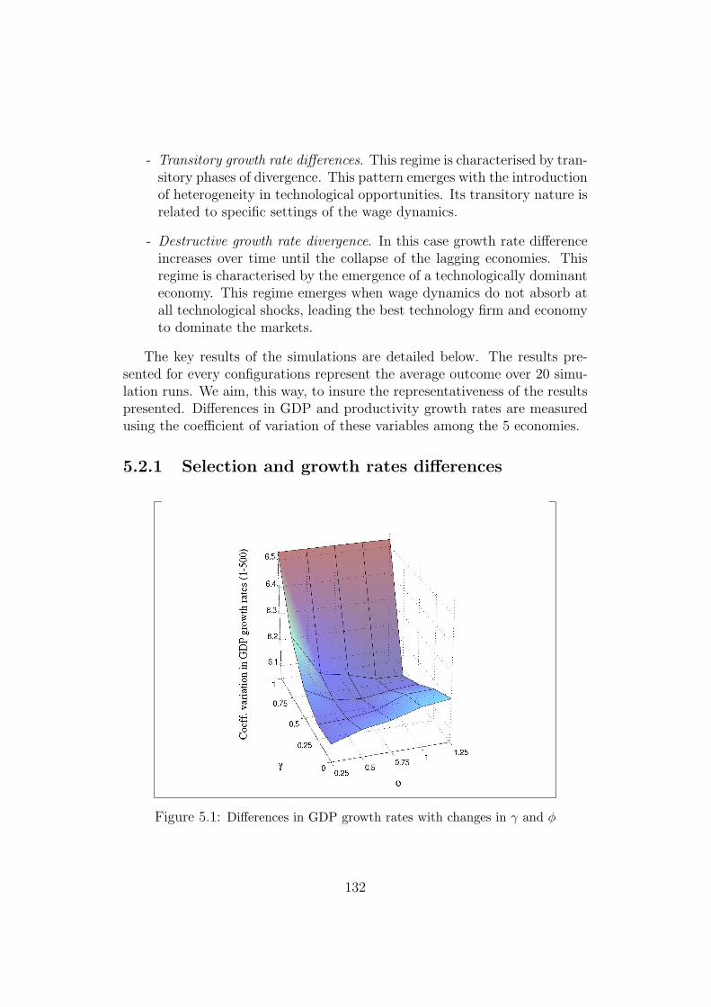
- Transitory growth rate differences. This regime is characterised by tran-sitory phases of divergence. This pattern emerges with the introductionof heterogeneity in technological opportunities. Its transitory nature isrelated to specific settings of the wage dynamics.
- Destructive growth rate divergence. In this case growth rate differenceincreases over time until the collapse of the lagging economies. Thisregime is characterised by the emergence of a technologically dominanteconomy. This regime emerges when wage dynamics do not absorb atall technological shocks, leading the best technology firm and economyto dominate the markets.
The key results of the simulations are detailed below. The results pre-sented for every configurations represent the average outcome over 20 simu-lation runs. We aim, this way, to insure the representativeness of the resultspresented. Differences in GDP and productivity growth rates are measuredusing the coefficient of variation of these variables among the 5 economies.
5.2.1 Selection and growth rates differences
Figure 5.1: Differences in GDP growth rates with changes in γ and φ
132
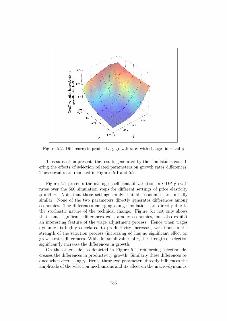
Figure 5.2: Differences in productivity growth rates with changes in γ and φ
This subsection presents the results generated by the simulations consid-ering the effects of selection related parameters on growth rates differences.These results are reported in Figures 5.1 and 5.2.
Figure 5.1 presents the average coefficient of variation in GDP growthrates over the 500 simulation steps for different settings of price elasticityφ and γ. Note that these settings imply that all economies are initiallysimilar. None of the two parameters directly generates differences amongeconomies. The differences emerging along simulations are directly due tothe stochastic nature of the technical change. Figure 5.1 not only showsthat some significant differences exist among economies, but also exhibitan interesting feature of the wage adjustment process. Hence when wagesdynamics is highly correlated to productivity increases, variations in thestrength of the selection process (increasing φ) has no significant effect ongrowth rates differences. While for small values of γ, the strength of selectionsignificantly increase the differences in growth.
On the other side, as depicted in Figure 5.2, reinforcing selection de-creases the differences in productivity growth. Similarly these differences re-duce when decreasing γ. Hence these two parameters directly influences theamplitude of the selection mechanisms and its effect on the macro-dynamics.
133
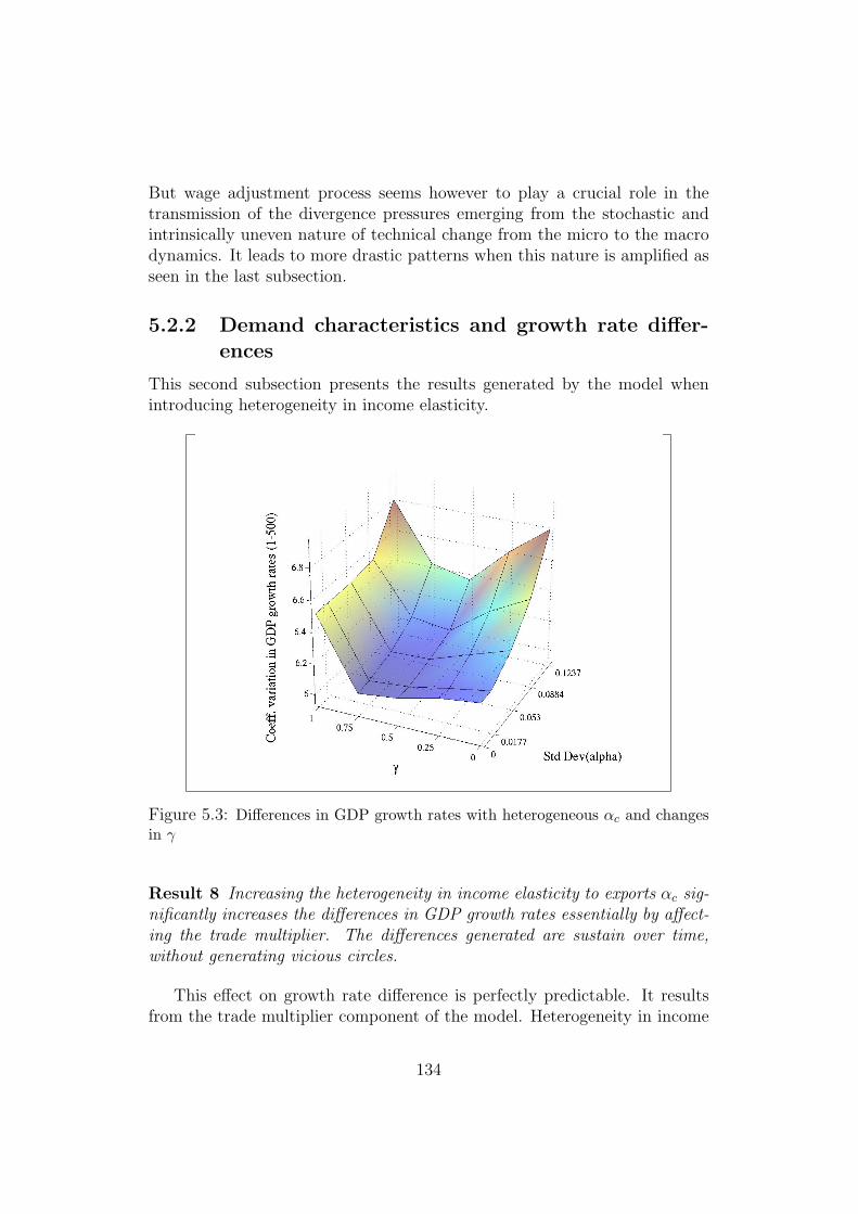
But wage adjustment process seems however to play a crucial role in thetransmission of the divergence pressures emerging from the stochastic andintrinsically uneven nature of technical change from the micro to the macrodynamics. It leads to more drastic patterns when this nature is amplified asseen in the last subsection.
5.2.2 Demand characteristics and growth rate differ-ences
This second subsection presents the results generated by the model whenintroducing heterogeneity in income elasticity.
Figure 5.3: Differences in GDP growth rates with heterogeneous αc and changesin γ
Result 8 Increasing the heterogeneity in income elasticity to exports αc sig-nificantly increases the differences in GDP growth rates essentially by affect-ing the trade multiplier. The differences generated are sustain over time,without generating vicious circles.
This effect on growth rate difference is perfectly predictable. It resultsfrom the trade multiplier component of the model. Heterogeneity in income
134
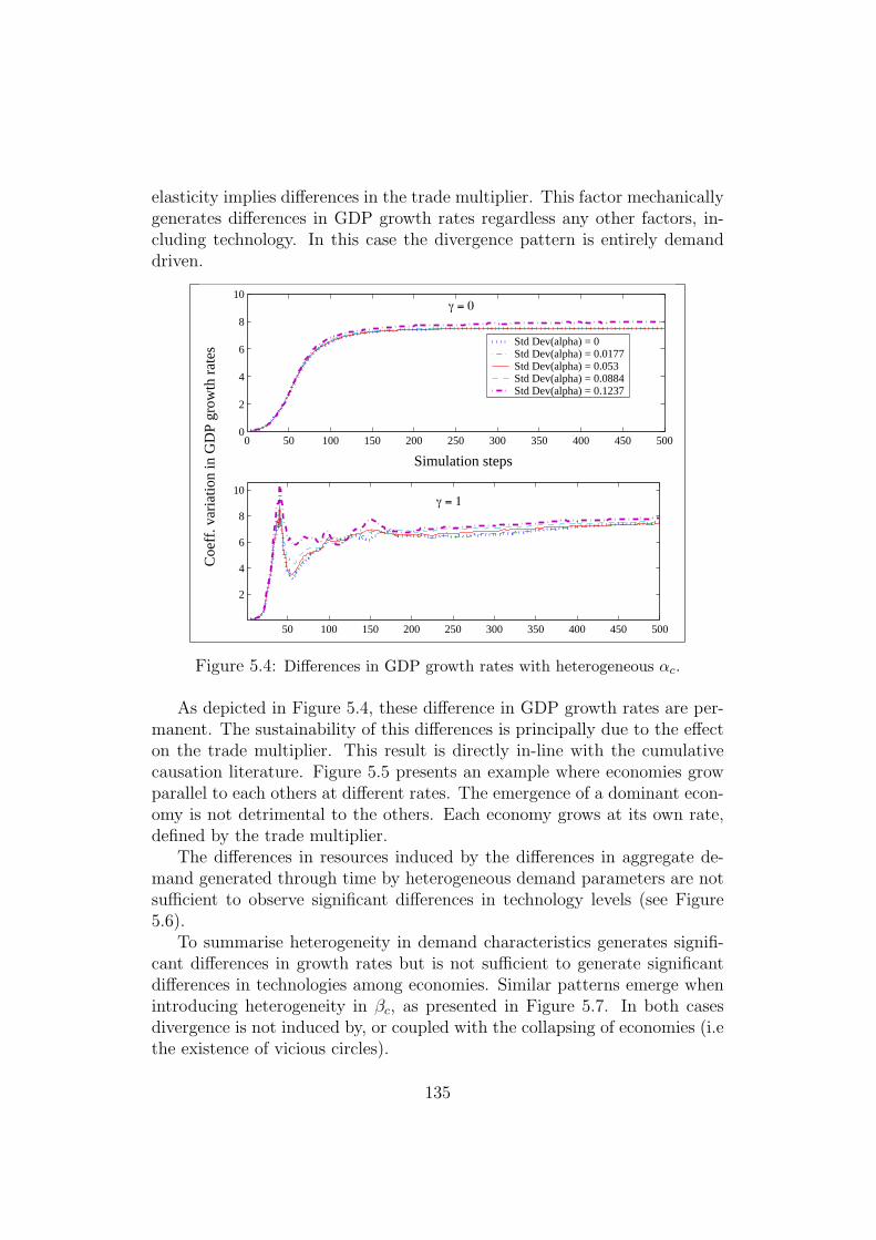
elasticity implies differences in the trade multiplier. This factor mechanicallygenerates differences in GDP growth rates regardless any other factors, in-cluding technology. In this case the divergence pattern is entirely demanddriven.
0 50 100 150 200 250 300 350 400 450 5000
2
4
6
8
10γ = 0
Simulation steps
50 100 150 200 250 300 350 400 450 500
2
4
6
8
10γ = 1
Coe
ff. v
aria
tion
in G
DP
grow
th r
ates
Std Dev(alpha) = 0Std Dev(alpha) = 0.0177Std Dev(alpha) = 0.053Std Dev(alpha) = 0.0884Std Dev(alpha) = 0.1237
Figure 5.4: Differences in GDP growth rates with heterogeneous αc.
As depicted in Figure 5.4, these difference in GDP growth rates are per-manent. The sustainability of this differences is principally due to the effecton the trade multiplier. This result is directly in-line with the cumulativecausation literature. Figure 5.5 presents an example where economies growparallel to each others at different rates. The emergence of a dominant econ-omy is not detrimental to the others. Each economy grows at its own rate,defined by the trade multiplier.
The differences in resources induced by the differences in aggregate de-mand generated through time by heterogeneous demand parameters are notsufficient to observe significant differences in technology levels (see Figure5.6).
To summarise heterogeneity in demand characteristics generates signifi-cant differences in growth rates but is not sufficient to generate significantdifferences in technologies among economies. Similar patterns emerge whenintroducing heterogeneity in βc, as presented in Figure 5.7. In both casesdivergence is not induced by, or coupled with the collapsing of economies (i.ethe existence of vicious circles).
135
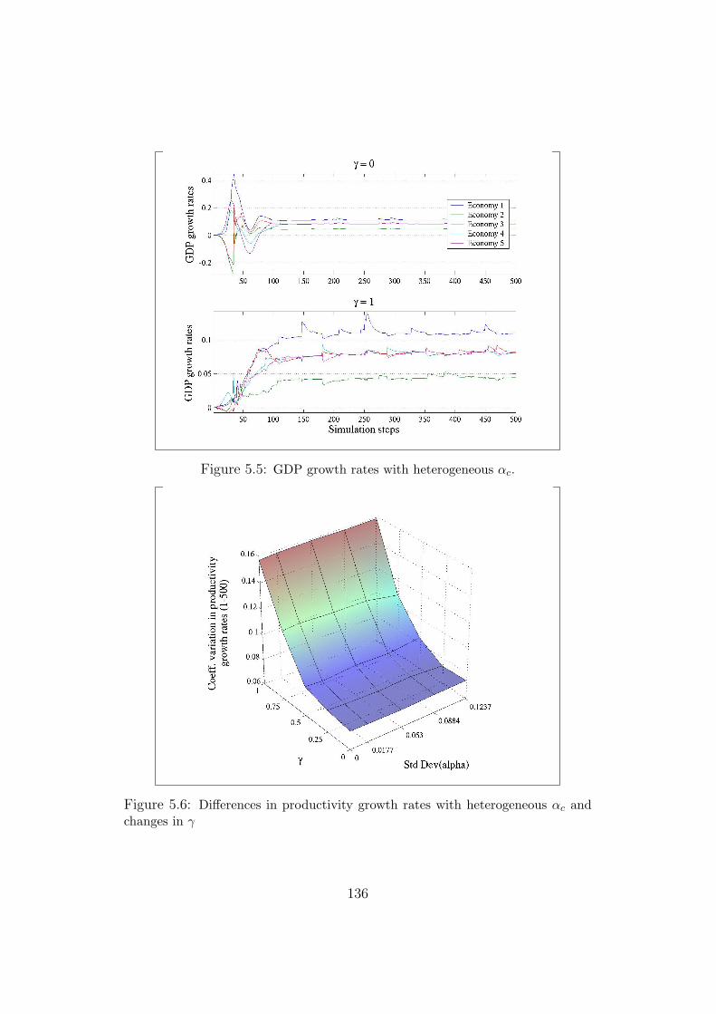
Figure 5.5: GDP growth rates with heterogeneous αc.
Figure 5.6: Differences in productivity growth rates with heterogeneous αc andchanges in γ
136
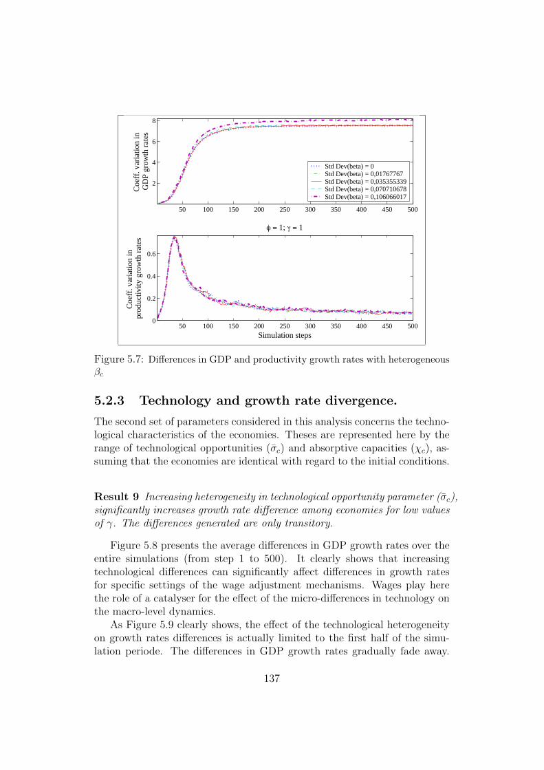
50 100 150 200 250 300 350 400 450 5000
0.2
0.4
0.6
φ = 1; γ = 1
Simulation steps
Coe
ff. v
aria
tion
in
prod
uctiv
ity g
row
th r
ates
50 100 150 200 250 300 350 400 450 500
2
4
6
8
Coe
ff. v
aria
tion
in
GD
P gr
owth
rat
es
Std Dev(beta) = 0 Std Dev(beta) = 0,01767767Std Dev(beta) = 0,035355339Std Dev(beta) = 0,070710678Std Dev(beta) = 0,106066017
Figure 5.7: Differences in GDP and productivity growth rates with heterogeneousβc
5.2.3 Technology and growth rate divergence.
The second set of parameters considered in this analysis concerns the techno-logical characteristics of the economies. Theses are represented here by therange of technological opportunities (σc) and absorptive capacities (χc), as-suming that the economies are identical with regard to the initial conditions.
Result 9 Increasing heterogeneity in technological opportunity parameter (σc),significantly increases growth rate difference among economies for low valuesof γ. The differences generated are only transitory.
Figure 5.8 presents the average differences in GDP growth rates over theentire simulations (from step 1 to 500). It clearly shows that increasingtechnological differences can significantly affect differences in growth ratesfor specific settings of the wage adjustment mechanisms. Wages play herethe role of a catalyser for the effect of the micro-differences in technology onthe macro-level dynamics.
As Figure 5.9 clearly shows, the effect of the technological heterogeneityon growth rates differences is actually limited to the first half of the simu-lation periode. The differences in GDP growth rates gradually fade away.
137
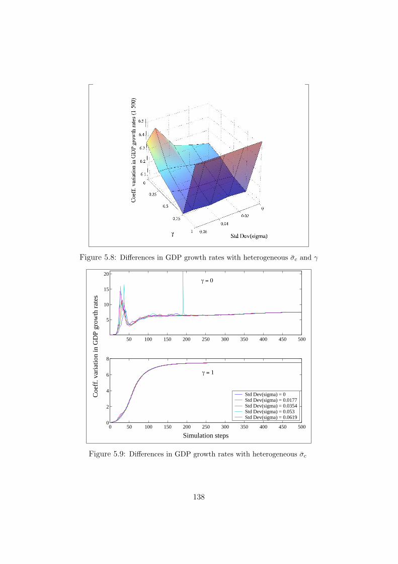
Figure 5.8: Differences in GDP growth rates with heterogeneous σc and γ
50 100 150 200 250 300 350 400 450 500
5
10
15
20γ = 0
0 50 100 150 200 250 300 350 400 450 5000
2
4
6
8
Simulation steps
Coe
ff. v
aria
tion
in G
DP
grow
th r
ates
γ = 1
Std Dev(sigma) = 0Std Dev(sigma) = 0.0177Std Dev(sigma) = 0.0354Std Dev(sigma) = 0.053Std Dev(sigma) = 0.0619
Figure 5.9: Differences in GDP growth rates with heterogeneous σc
138
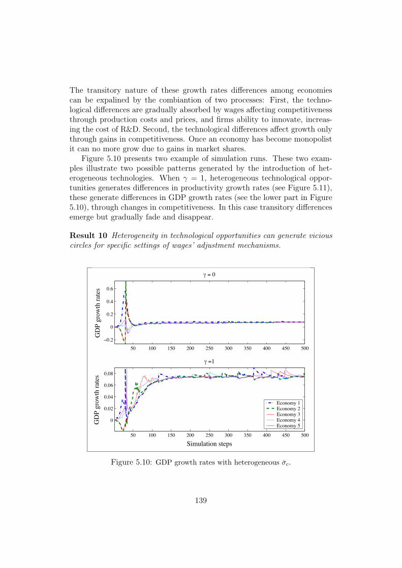
The transitory nature of these growth rates differences among economiescan be expalined by the combiantion of two processes: First, the techno-logical differences are gradually absorbed by wages affecting competitivenessthrough production costs and prices, and firms ability to innovate, increas-ing the cost of R&D. Second, the technological differences affect growth onlythrough gains in competitiveness. Once an economy has become monopolistit can no more grow due to gains in market shares.
Figure 5.10 presents two example of simulation runs. These two exam-ples illustrate two possible patterns generated by the introduction of het-erogeneous technologies. When γ = 1, heterogeneous technological oppor-tunities generates differences in productivity growth rates (see Figure 5.11),these generate differences in GDP growth rates (see the lower part in Figure5.10), through changes in competitiveness. In this case transitory differencesemerge but gradually fade and disappear.
Result 10 Heterogeneity in technological opportunities can generate viciouscircles for specific settings of wages’ adjustment mechanisms.
50 100 150 200 250 300 350 400 450 500
−0.2
0
0.2
0.4
0.6
GD
P gr
owth
rat
es
γ = 0
50 100 150 200 250 300 350 400 450 500
0
0.02
0.04
0.06
0.08
Simulation steps
GD
P gr
owth
rat
es
γ =1
Economy 1Economy 2Economy 3Economy 4Economy 5
Figure 5.10: GDP growth rates with heterogeneous σc.
139
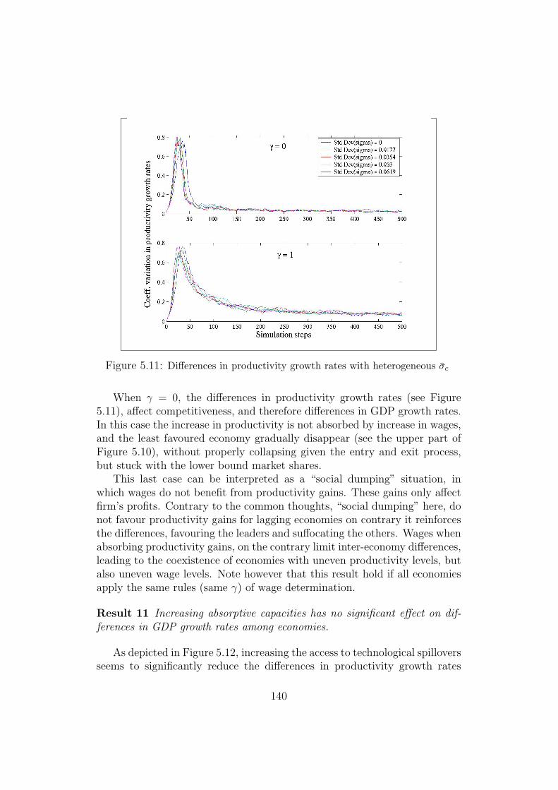
Figure 5.11: Differences in productivity growth rates with heterogeneous σc
When γ = 0, the differences in productivity growth rates (see Figure5.11), affect competitiveness, and therefore differences in GDP growth rates.In this case the increase in productivity is not absorbed by increase in wages,and the least favoured economy gradually disappear (see the upper part ofFigure 5.10), without properly collapsing given the entry and exit process,but stuck with the lower bound market shares.
This last case can be interpreted as a “social dumping” situation, inwhich wages do not benefit from productivity gains. These gains only affectfirm’s profits. Contrary to the common thoughts, “social dumping” here, donot favour productivity gains for lagging economies on contrary it reinforcesthe differences, favouring the leaders and suffocating the others. Wages whenabsorbing productivity gains, on the contrary limit inter-economy differences,leading to the coexistence of economies with uneven productivity levels, butalso uneven wage levels. Note however that this result hold if all economiesapply the same rules (same γ) of wage determination.
Result 11 Increasing absorptive capacities has no significant effect on dif-ferences in GDP growth rates among economies.
As depicted in Figure 5.12, increasing the access to technological spilloversseems to significantly reduce the differences in productivity growth rates
140
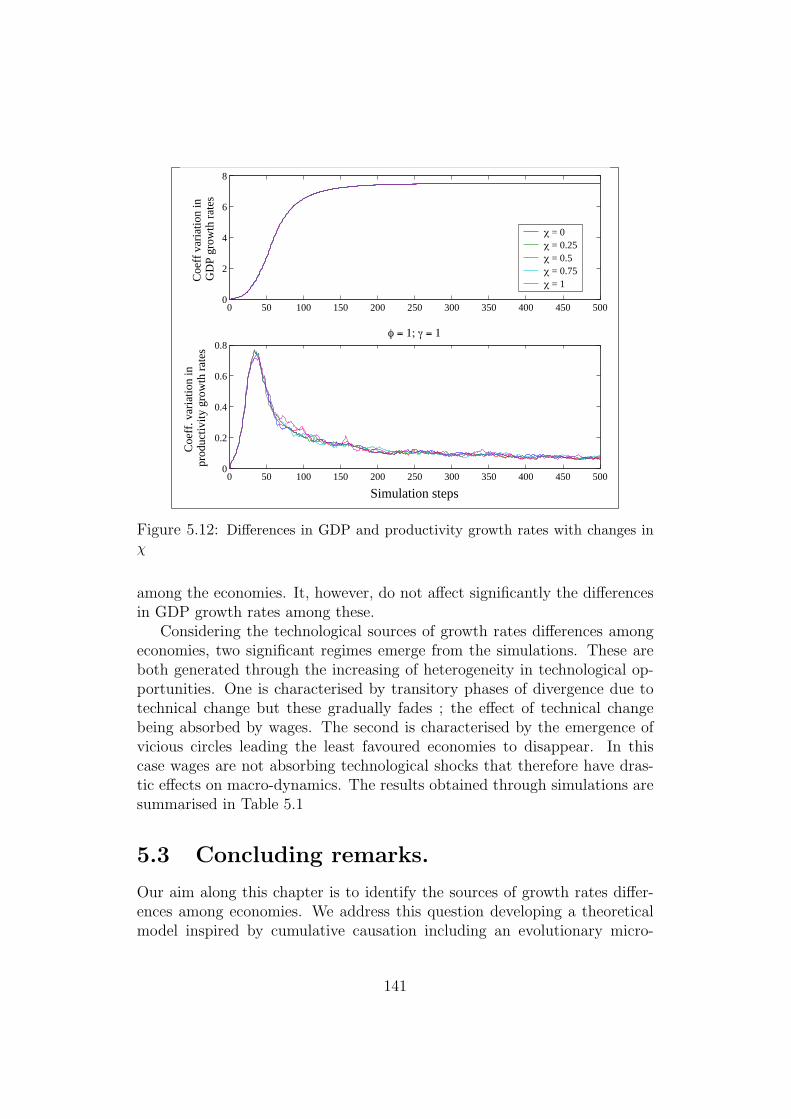
0 50 100 150 200 250 300 350 400 450 5000
2
4
6
8
Coe
ff v
aria
tion
in
GD
P gr
owth
rat
es
0 50 100 150 200 250 300 350 400 450 5000
0.2
0.4
0.6
0.8φ = 1; γ = 1
Simulation steps
Coe
ff. v
aria
tion
in
prod
uctiv
ity g
row
th r
ates
χ = 0χ = 0.25χ = 0.5χ = 0.75χ = 1
Figure 5.12: Differences in GDP and productivity growth rates with changes inχ
among the economies. It, however, do not affect significantly the differencesin GDP growth rates among these.
Considering the technological sources of growth rates differences amongeconomies, two significant regimes emerge from the simulations. These areboth generated through the increasing of heterogeneity in technological op-portunities. One is characterised by transitory phases of divergence due totechnical change but these gradually fades ; the effect of technical changebeing absorbed by wages. The second is characterised by the emergence ofvicious circles leading the least favoured economies to disappear. In thiscase wages are not absorbing technological shocks that therefore have dras-tic effects on macro-dynamics. The results obtained through simulations aresummarised in Table 5.1
5.3 Concluding remarks.
Our aim along this chapter is to identify the sources of growth rates differ-ences among economies. We address this question developing a theoreticalmodel inspired by cumulative causation including an evolutionary micro-
141
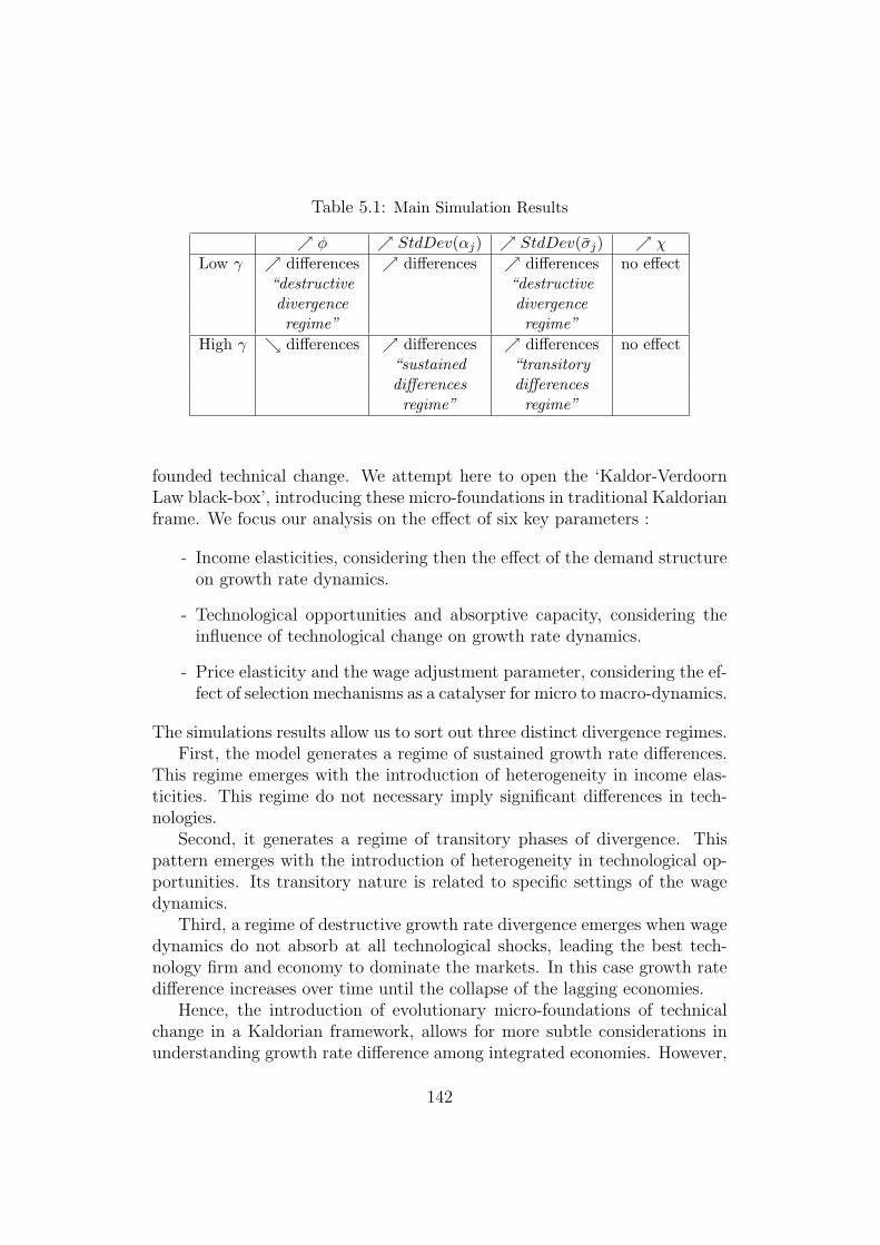
Table 5.1: Main Simulation Results
↗ φ ↗ StdDev(αj) ↗ StdDev(σj) ↗ χ
Low γ ↗ differences ↗ differences ↗ differences no effect“destructive “destructivedivergence divergenceregime” regime”
High γ ↘ differences ↗ differences ↗ differences no effect“sustained “transitorydifferences differencesregime” regime”
founded technical change. We attempt here to open the ‘Kaldor-VerdoornLaw black-box’, introducing these micro-foundations in traditional Kaldorianframe. We focus our analysis on the effect of six key parameters :
- Income elasticities, considering then the effect of the demand structureon growth rate dynamics.
- Technological opportunities and absorptive capacity, considering theinfluence of technological change on growth rate dynamics.
- Price elasticity and the wage adjustment parameter, considering the ef-fect of selection mechanisms as a catalyser for micro to macro-dynamics.
The simulations results allow us to sort out three distinct divergence regimes.First, the model generates a regime of sustained growth rate differences.
This regime emerges with the introduction of heterogeneity in income elas-ticities. This regime do not necessary imply significant differences in tech-nologies.
Second, it generates a regime of transitory phases of divergence. Thispattern emerges with the introduction of heterogeneity in technological op-portunities. Its transitory nature is related to specific settings of the wagedynamics.
Third, a regime of destructive growth rate divergence emerges when wagedynamics do not absorb at all technological shocks, leading the best tech-nology firm and economy to dominate the markets. In this case growth ratedifference increases over time until the collapse of the lagging economies.
Hence, the introduction of evolutionary micro-foundations of technicalchange in a Kaldorian framework, allows for more subtle considerations inunderstanding growth rate difference among integrated economies. However,
142

this model might constitute the starting point for further analysis. The waytechnical change is considered remains sketchy.
Simulations also highlight the crucial role played by the wage adjustmentmechanisms as a catalyser for growth impulses from micro to macro. Similarresults were found concerning the relationship between specialisation andgrowth differences in a multi-sectorial extension of this model developed inChapter 6. Distinct regimes emerge, demand and technology driven. Thereagain, the wage adjustment process allows the transmission of micro-shocksto macro-dynamics.
143

Simulation Settings
Table 5.2: Key parameters settings (the values by default are in italic)
Economy 1 Economy 2 Economy 3 Economy 4 Economy 5αj 0,375 0,375 0,375 0,375 0,375αj 0,4 0,35 0,375 0,375 0,375αj 0,45 0,3 0,375 0,375 0,375αj 0,5 0,25 0,375 0,375 0,375αj 0,55 0,2 0,375 0,375 0,375βj 0,5 0,5 0,5 0,5 0,5βj 0,525 0,475 0,5 0,5 0,5βj 0,55 0,45 0,5 0,5 0,5βj 0,6 0,4 0,5 0,5 0,5βj 0,65 0,35 0,5 0,5 0,5σj 0,1 0,1 0,1 0,1 0,1σj 0,125 0,075 0,1 0,1 0,1σj 0,15 0,05 0,1 0,1 0,1σj 0,175 0,025 0,1 0,1 0,1σj 0,1875 0,0125 0,1 0,1 0,1χj 0 0 0 0 0χj 0,25 0,25 0,25 0,25 0,25χj 0,5 0,5 0,5 0,5 0,5χj 0,75 0,75 0,75 0,75 0,75χj 1 1 1 1 1γ 0 0 0 0 0γ 0,25 0,25 0,25 0,25 0,25γ 0,5 0,5 0,5 0,5 0,5γ 0,75 0,75 0,75 0,75 0,75γ 1 1 1 1 1φ 0,25 0,25 0,25 0,25 0,25φ 0,5 0,5 0,5 0,5 0,5φ 0,75 0,75 0,75 0,75 0,75φ 1 1 1 1 1φ 1,25 1,25 1,25 1,25 1,25
144
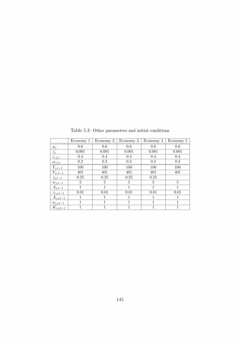
Table 5.3: Other parameters and initial conditions
Economy 1 Economy 2 Economy 3 Economy 4 Economy 5µj 0.6 0.6 0.6 0.6 0.6zj 0.001 0.001 0.001 0.001 0.001ιi,j,c 0.4 0.4 0.4 0.4 0.4ρi,j,c 0.2 0.2 0.2 0.2 0.2Yc,t−1 100 100 100 100 100Yw,t−1 401 401 401 401 401zj,t−1 0.25 0.25 0.25 0.25wj,t−1 5 5 5 5 5Aj,t−1 1 1 1 1 1zi,j,t−1 0.01 0.01 0.01 0.01 0.01Ai,j,t−1 1 1 1 1 1ai,j,t−1 1 1 1 1 1Ki,j,t−1 1 1 1 1 1
145

146
Chapter 6
Sectoral Specialisation andGrowth Rate Differences
This chapter1 follows the same theoretical frame then Chapter 5. We usethe framework developed in this chapter to consider the possible relationshipbetween patterns of sectoral specialisation and growth rate differences amongeconomies.
Both empirical and theoretical literature on growth recently put forwardthe argument that sectoral specialisation can explain patterns in growthrate differences among economies. Dalum, Laursen and Verspagen (1999),Laursen (2000) and Meliciani (2001) present empirical evidences that spe-cialisation affects growth. Specialisation patterns are linked to the compet-itiveness of the economies in the various sectors. They then affect growthrate differences due to the existence of differences in the growth potential ofeach sectors. Some models can be found in the literature trying to reproducethese facts : Among others, Verspagen (1993), Cimoli (1994), Dosi, Fabi-ani, Aversi and Meacci (1994) and Los and Verspagen (2003). Verspagen(1993), Cimoli (1994) and Los and Verspagen (2003) connect specialisationpatterns to the existence of structural differences in productivity dynam-ics among sectors and economies. The effect of specialisation patterns onGDP growth rate differences derives from demand characteristics: incomeelasticity (Verspagen (1993) and Cimoli (1994)) or income elasticity plusthe industrial input-output structure (Los and Verspagen (2003)). Dosi,Fabiani, Aversi and Meacci (1994), develop an evolutionary micro-foundedmulti-sectoral multi-country model. Authors conclude that these patterns ofsectoral specialisation and GDP growth rate divergence generated by theirmodel emerge from the interaction of micro-heterogeneity in behaviours and
1This chapter draws upon the model and simulation results presented in Lorentz (2004).
147
technological dynamics with the market selection mechanisms. Our modelproposes an intermediate approach.
We develop a multi-sectoral growth model that links a Kaldorian macro-framework to an evolutionary modelling of technical change and industrialdynamics. In this sense we add a meso-level of analysis to the baseline modelpresented in Chapter 5
This chapter is organised as follows: The next section is devoted to thepresentation of the model. Section 6.2 reports the main results emergingfrom simulations and their interpretations.
6.1 A Multi-Sectoral Growth Model.
This section presents a multi-sectoral extension to the growth model we pro-posed in the previous chapter. It considers economic growth as a demand-led process along Kaldorian lines. Economic growth is driven by externaldemand through a multiplier effect and technological change. These causalrelationships are formally deduced from the balance of payment constraint.
Technical change emerges from the micro-dynamics following the evo-lutionary tradition. These replace the Kaldor-Verdoorn Law traditionallyfound in the Kaldorian literature.
Macro and micro-dynamics are strongly interrelated. Aggregate demandprovides the necessary resources to finance firms’ technological developmentand therefore their competitiveness. Selection among firms and among sec-tors is also rooted in macro-dynamics through demand and wage settingmechanisms. Hence the macro-evolution generates the resources of the firmsand the mechanisms ensuring their redistribution among the latter. In thissense the macro-frame constraints the micro-dynamics.
On the other side micro-dynamics are the core of technological change,one of the engines of growth. The competitiveness of economies relies onnational firms’ ability to gain productivity.
These channels constitute the circular causality between macro and micro-dynamics, driving the entire long-run growth processes.
The structure of the model can be described as follows: We consider a setof C economies integrated in an economic system through trade relations.An economy c ∈ [1; C], is referred to with the index c. When variables areindexed w, they concern the foreign economies with regard to the economyc.
Our system counts J sectors of activity. Each economy can produce andconsume products of each of these sectors. A sector j ∈ [1; J ], is referred to
148
using the index j.For each economy, I firms are active in each of the J sectors. A firm
i ∈ [1; I], producing in sector j and based in the economy c is referred towith the indexes i, j, c.
The entire economic system then counts C economies, J sectors, andC ∗ J ∗ I firms. The index t refers to the time step.
6.1.1 The macro-economic framework: Internationaltrade, economic growth, and wage dynamics.
This subsection presents the macro-economic framework of the model. Thelatter is decomposed in two distinct processes. First we consider GDP dy-namics as deduced from the balance of payment constraint. Second, we definewage dynamics as correlated to labour productivity dynamics.
We assume that the considered economies are part of an integrated mon-etary system. We then excluded monetary adjustment to possible tradedisequilibria. This is the case if considering as unit of analysis regions orcountries in a single currency area. Economies being subject to balance ofpayment constraint, it thus implies that imports equal exports. Given thefunctional representation of imports and exports, as developed below, we canthen deduce the GDP dynamics from the balance of payment constraint.
The macro-economic framework we developed here is directly rooted inthe formal interpretations of Kaldor’s cumulative causation approach of theeconomic growth process. Our formal representation found its inspiration inthis respect in Thirlwall (1979) model, or in the more recent multi-sectoralmodels by Cimoli (1994) or Verspagen (1993), among others.
Balance of payment constraint and the determination of aggregatedemand:
For each sector j of an economy c, exports are defined as follows:
Xj,c,t = sj,w,t(Yw,t)αczj,c,t (6.1)
where Yw,t represents the GDP of the rest of the world, computed as thesum of GDP levels of all foreign economies, zj,c,t represents the market shareof the economy on the international markets for the sector j. αc is theincome elasticity of the rest of the world with respect to economy c exports.sj,w,t represents the share of income devoted to the consumption of sector jproducts by the rest of the world. It is formally computed as follows:
sj,w,t =Y
εj
w,t
Yw,t
149
Where εj represents the income elasticity of sector j products’ consumption.The market share of the economy in a sector is a proxy for the price
competitiveness of the economy in the sector. It is given by the sum of themarket shares of the domestic firms active in this sector:
zj,c,t =∑
i
zi,j,c,t
Each firm’s market shares is defined through a replicator dynamic, functionof firm’s relative competitiveness. Hence the market share of each firm willbe computed as follows:
zi,j,c,t = zi,j,c,t−1
(1 + φ
(Ei,j,c,t
Ej,t
− 1
))(6.2)
where zi,j,c,t represents the market share of firm i, pi,j,c,t the price of itsproduct. Ei,j,c,t stands for firm i, in sector j level of competitiveness:
Ei,j,c,t =1
pi,j,c,t
Ej,t, the average competitiveness on the international market, is computedas follows:
Ej,t =∑c,i
zi,j,c,t−1Ei,j,c,t
The parameter φ measures the reactivity of the selection mechanism tocompetitiveness. Given our specification this parameter can be interpretedas a measure of price elasticity.
Imports follow the exports’ specification scheme. They are function of do-mestic economy income, of domestic share of consumption of sector j goods,and of the rest of the world’s market share. Formally imports are computedas follows:
Mj,c,t = sj,c,t(Yc,t)βc(1− zj,c,t) (6.3)
With
sj,c,t =Y
εj
c,t
Yc,t
sj,c,t represents the share of income devoted to the consumption of the prod-ucts of sector j sector. Note that εj, the income elasticity of consumptionof sector j products is fixed and equal across economies. The parameter βc
represents the income elasticity to import. Yc,t represents aggregate demandwhich, given the demand-led nature of the model, also defines GDP.
150
The growth rate of exports and imports for each sector can be deducedfrom these expressions as :
∆Xj,c,t
Xj,c,t−1
= (αc + εj − 1)∆Yw,t
Yw,t−1
+ φ
(Ej,c,t
Ej,t
− 1
)(6.4)
∆Mj,c,t
Mj,c,t−1
= (βc + εj − 1)∆Yc,t
Yc,t−1
− bj,c,t−1φ
(Ej,c,t
Ej,t
− 1
)(6.5)
withbj,c,t−1 =
zj,c,t−1
1− zj,c,t−1
External trades are subject to balance of payment constraint. Hence thegrowth rate of exports has to equal growth rate of imports. Thus:
∆Xc,t
Xc,t−1
=∆Mc,t
Mc,t−1
(6.6)
WithXc,t =
∑j
pj,c,tXj,c,t and Mc,t =∑j
pmj,c,tMj,c,t
pj,c,t =∑
i
pi,j,c,tzi,j,c,t
zj,c,t
and pmj,c,t =
∑c 6=c
∑i
pi,j,c,tzi,j,c,t
1− zj,c,t
The balance of payment constraint can be rewritten as follows:
∑j
ij,c,t−1∆Mj,c,t
Mj,c,t−1
+∑j
ij,c,t−1
∆pmj,c,t
pmj,c,t−1
=∑j
ej,c,t−1∆Xj,c,t
Xj,c,t−1
+∑j
ej,c,t−1∆pj,c,t
pj,c,t−1
(6.7)where:
ij,c,t−1 =pm
j,c,t−1sj,c,t−1(1− zj,c,t−1)∑j pm
j,c,t−1sj,c,t−1(1− zj,c,t−1)and ej,c,t−1 =
pj,c,t−1sw,j,t−1zj,c,t−1∑j pj,c,t−1sw,j,t−1zj,c,t−1
ij,c,t−1 and ej,c,t−1 weigh the importance of each sector’ s dynamics in grossimports and exports dynamics. These two components reflect the sectoralstructure of the economy. Their changes through time illustrate the struc-tural changes in the economies.
The introduction of the balance of payment constraint allows us to expressthe GDP growth rate as function of the rest of the world GDP growth rate and
151
of market share growth rate. Formally GDP growth rate will be computedas follows:
∆Yc,t
Yc,t−1
= γc,t−1∆Yw,t
Yw,t−1
+ λc,t−1φ
∑j
θj,c,t−1
(Ej,c,t
Ej,t
− 1
)+ λc,t−1
∑j
κj,c,t−1
(6.8)With
γc,t−1 =αc +
∑j ej,c,t−1εj − 1
β +∑
j ij,c,t−1εj − 1(6.9)
λc,t−1 =1
β +∑
j ij,c,t−1εj − 1(6.10)
θj,c,t−1 = ej,c,t−1 + ij,c,t−1bj,c,t−1 (6.11)
κj,c,t−1 = ej,c,t−1∆pj,c,t
pj,c,t−1
− ij,c,t−1
∆pmj,c,t
pmj,c,t−1
(6.12)
The first component of the right hand side of the equation captures a trademultiplier like effect on GDP growth rates. The second and third componentsmirror the effects of technological change on GDP dynamics through respec-tively the linkage between sectoral competitiveness and GDP growth, andbetween price changes and GDP growth. This representation allows a cleardecomposition between the effect of external demand and of technologicalchange on the ‘short-run’ GDP dynamics. The relative weight of these com-ponents is strongly linked to the structural characteristics of the economy.These characteristics are themselves subject to changes along time, due tothe evolution of demand and technological change, leading to more complexinteractions in defining the long-run growth patterns than in this short-runspecification.
Wage determination:
Wages are set at the sectoral level. For a given sector j wage dynamics willbe correlated to sector j productivity growth rate ( ∆Aj,c,t
Aj,c,t−1) and to the entire
economy productivity growth rate ( ∆Ac,t
Ac,t−1). The effect of these two variables
on wage dynamics is weighted by the parameter ν ∈ [0; 1], such that :
- When ν = 1, the wage dynamics for every sector only depend on themacro-level productivity growth rate. (i.e. as a centralised wage nego-tiation system)
- When ν = 0, the wage dynamics for every sector only depend on thesector-level productivity growth rate. (i.e. as a sectoral wage negotia-tion system)
152
Wage dynamics of the sector j, in the economy c is represented as follows:
∆wj,c,t
wj,c,t−1
= ν∆Ac,t
Ac,t−1
+ (1− ν)∆Aj,c,t
Aj,c,t−1
(6.13)
With
Ac,t =Yc,t
Lc,t
and Aj,c,t =Yj,c,t
Lj,c,t
Note that the wage level defined with this process during the period t is ap-plied by firms at period t + 1. Wage dynamics in our model act as a secondmacro-constraint on firms. Hence, it affects directly firms competitivenessand then the effect of the selection mechanisms on firms. Firms in a givensector of an economy will loose competitiveness if their own productivitygrowth rate is slower then the average one. Moreover, when ν 6= 0, wagedynamics generate a selection process among sectors. Hence, if the averageproductivity of a sector grows slower then the average productivity growthrate of the entire economy, through wage dynamics, this sector looses com-petitiveness. The amplitude of this effect directly depends on the value ofthe parameter ν. As argued in the last section of this paper wage dynamicsthrough the process described above play a major role in the specialisationdynamics.
6.1.2 Firms: production, construction of productioncapacity
This subsection is devoted to the description of the microeconomic level ofthe model. We consider here the formal representation of firms’ productioncapacities, investment decisions and R&D activity. Note that the representa-tion provided is common to all sectors and economies. Sectoral or economy-wide specificity, when considered, takes the form of specific parameter values.Formally the micro-level of this model is similar to the one found in the pre-vious chapter. Hence, following the evolutionary tradition we consider apopulation of bounded rational firms that can differ in their technologicalcharacteristics and behaviours. Technical change emerges at the firm level asa mutation process. More precisely technical change is embodied in capitalvintages developed by firms to build and improve their production capacities.
Firms then play two specific role in the model. First they satisfy thedemand needs. This provides them with the necessary resources to sustainthe development of their production capacities. Second, through this processthey generate technical change. The latter then affects the macro-dynamics,increasing the economy competitiveness and therefore affects demand dy-namics.
153
Production and pricing:
Firms’ production process is represented by a Leontiev production functionwith labour as unique production factor. Capital goods enter the produc-tion function in defining labour productivity. The production function isrepresented as follows :
Yi,j,c,t = Ai,j,c,t−1Lpi,j,c,t (6.14)
where Yi,j,c,t is the output of firm i, producing in sector j at time t. Ai,j,c,t−1
represents labour productivity and Lpi,j,c,t the labour force employed in the
production process. Output is constrained by the demand directed to thefirms and defined at the macro-economic level. The level of production ofeach firm is computed as a share of sector j demand2 given by their relativemarket share such as:
Yi,j,c,t =zi,j,c,t
zj,c,t
Yj,c,t
Labour productivity is function of the firms’ accumulation of capitalgoods. Each capital good embodies a level of labour productivity. Investmentin the different vintages of capital goods modifies the labour productivity ofthe firm. Hence, at the end of any period t, we define the level of labourproductivity as follows:
Ai,j,c,t =Ii,j,c,tai,j,c,t−1∑t
τ=1 Ii,j,c,τ
+
∑t−1τ=1 Ii,j,c,τ∑tτ=1 Ii,j,c,τ
Ai,j,c,t−1 (6.15)
where ai,j,c,t−1 represent the labour productivity embodied in the capital gooddeveloped by the firm i during the period t− 1. Ii,j,c,t represents the level ofinvestment in capital goods of the firm.
Firms set prices through a mark-up process. This mark-up is appliedto unitary production costs, corresponding here to labour costs. Prices arecomputed as follows:
pi,j,c,t = (1 + µj)wc,t−1
Ai,j,c,t−1
(6.16)
where pi,j,c,t represents the price set by firm i at time t, µj the mark-up co-efficient and wj,t−1 the wage level set at the macro level for the entire sector.Note that we assume here that the mark-up coefficients are fixed for eachfirm in a given sector of a given economy.
2Sector j demand is computed as: Yj,c,t = Xj,c,t + sj,c,t(1− (Yc,t)βc−1)Yc,tzj,c,t.
154
Firm’s profit level will then be computed as follows:
Πi,j,c,t = pi,j,c,tYi,j,c,t − wj,c,t−1Lpi,j,t = µj
wj,c,t−1
Ai,j,c,t−1
Yi,j,c,t (6.17)
Profits constitute in the model the only financial resource for firms’ invest-ments.
Building production capacities:
As introduced previously, to build but also improve their production capac-ities, firms have to accumulate capital vintages. Each capital good is devel-oped in-house by firms and then introduced in their production technologies.This process is decomposed in two phases. First firms explore and developnew capital goods, through local search or through the adaptation of exist-ing capital goods to their own production techniques. This phase takes placewithin the R&D activity of the firms. The latter is financed by investmentsin R&D. The second stage consists in introducing the outcome of the R&Dactivity within the production process. This stage is costly and requires firmsto invest in the exploitation of the latest capital good vintage. The level ofinvestment determines the relative importance of the latest capital goods inthe production process and therefore determines the effective productivitygains, as described above. These two distinct investments are subject to thefirms financial constraint. Firms’ only resources for investments are theirprofits. More profitable firms are more inclined to invest and therefore toimprove their production capacities and their competitiveness.
The investment decision timing is set as follows, first firms invest in capitalgoods, in order to gain from the already developed vintages, and then investin R&D. Investment in capital goods corresponds to a share ιi,j,c of firms’sales. Given the financial constraint the investment level in capital good isformally represented as follows:
Ii,j,c,t = min {ιi,j,cYi,j,c,t ; Πi,j,c,t} (6.18)
Investments in R&D are a share ρi,j,c of their sales. R&D investment willcorrespond to the hiring of workers assigned to the research activity :
Ri,j,c,t =1
wj,c,t−1
min{ρi,j,cYi,j,c,t; Πi,j,c,t − Ii,j,c,t} (6.19)
The formal representation of the R&D process is explicitly inspired byevolutionary modelling of technical change. Hence following Nelson and Win-ter (1982) we will consider that the probability of success of research is an
155
increasing function of R&D investments. Formally the R&D activity is rep-resented by the following algorithm:
1. Firms draw a number from a Uniform distribution on [0 ; 1].
2. If this number is contained in the interval [0 ; Ri,j,c,t
Yi,j,c,t], the R&D is
successful. Hence a new capital good vintage has been developed.
3. If R&D is successful, its outcome is drawn from the following distri-bution. We differentiate here explicitly innovative firms from imitativeones:
ai,j,c,t = max {ai,j,c,t−1 + εi,j,c,t; ai,j,c,t−1} (6.20)
εi,j,c,t ∼ N(0; σi,j,c,t) (6.21)
with
{σi,j,c,t = σj,c if the firm is an innovatorσi,j,c,t = χj,c(aj,t − ai,j,c,t) if the firm is an imitator
(6.22)
The outcome of the R&D process defines the labour productivity levelembodied in the newly discovered capital vintage (ai,j,c,t). aj,t represents theaverage productivity level embodied in the latest capital vintages developedby firms. It is formally computed as:
aj,t =∑i,c
zi,j,c,tai,j,c,t−1
Hence aj,t−ai,j,c,t represents firm i, j, c technological gap, while the parameterχj,c ∈ [0; 1] can be seen as the degree of access to spillover for the imitatingfirms.
Firms exit the market if their market share is lower then zj. They arereplaced by firms with a productivity level and value of the latest capitalvintage developed equal to the average values of these variables within thesector and economy of the exiting firms and a market share equal to zj. Inthis respect the number of firms remains constant. An exiting innovatoris replaced by an entrant innovator, and an exiting imitator by an entrantimitator. The proportion of innovators, and thus imitators, then remainsconstant.
156
6.2 Sectoral Specialisation and Growth Rate
Differences: Main Simulation Results
The model, as detailed in the previous section, is developed to consider thedeterminants of sectoral specialisation and their effect on growth rate differ-ences among the integrated economies. We do not assume here any ad-hocspecialisation. We rather look for specialisation to emerge from the dynamicsgenerated through the model.
Some models can be found in the literature that raise the question of theemergence of specialisation patterns. Due to some similarities on the theo-retical ground, one might particularly think about Verspagen (1993), Aversi,Dosi, Fabiani and Meacci (1994), Cimoli (1994) or Los and Verspagen (2003)among others. Verspagen (1993), Cimoli (1994) and Los and Verspagen(2003) connect specialisation patterns to the structural differences amongeconomies in the sources of technical change and productivity gain. Theybase their analysis on the Kaldor-Verdoorn Law. These models then link spe-cialisation patterns to GDP growth rate differences through the differences inincome elasticity of sectors’ demand. In this respect these models are close tothe Kaldorian analysis of growth rate differences. Dosi, Fabiani, Aversi andMeacci (1994), develop an evolutionary micro-founded multi-sectoral growthmodel. They show the emergence of significant patterns of GDP growth ratedivergence among economies. These can be coupled to sectoral specialisationpatterns in some economies. Authors conclude that these patterns emergefrom the interaction of micro-heterogeneity in behaviours and technologicaldynamics with the market selection mechanisms. They thus consider thesepatterns as micro-driven.
We consider here economies initially identical, endowed with the samepotentials of productivity growth, and equal access to spillovers. Technolog-ical heterogeneity among firms and therefore economies in our model resultsfrom the stochastic generation of technical change at the micro-level.
As for most of the models incorporating evolutionary features, we need toresort to numerical simulations.3 Simulations are set through the followingscheme. Our artificial system counts 4 economies and 5 industrial sectors.Each economy is producing and consuming the output of each of these sec-tors and counts 20 active firms per sectors. An economy is then composedof 100 firms, and each sector counts 80 firms competing against each others.In each sector, and each country half of the firms are set being innovators
3Simulations are implemented using the Laboratory for Simulation Development (LSD)environment. See Valente and Andersen (2002)
157
and therefore half of them are imitators. Exiting innovators are replaced byentering innovators, so that this proportion remains constant. All firms andall economies are initially similar, in terms of initial conditions and parame-ter settings.These settings are detailed in Tables 6.2, 6.3 and ??.
Our analysis focuses on the effect of two groups of parameters. A firstone concerns macro-components of the model, while the second considerstechnological parameters. The macro-level parameters are the following:
- ν, the parameter weighting the effect of sector versus aggregate produc-tivity growth rates in the sector-level wage dynamics. This parametergenerates a selection among sectors, favouring the most dynamic onesin terms of productivity increases, through the relationship betweenwage and prices and therefore competitiveness.
- φ, the price elasticity, included in the replicator equation, directly influ-ences the speed of the selection process among firms in a given sector.This parameter should somehow regulate the amplitude of the special-isation process.
- εj, for which we consider the effect of growing inter-sector heterogeneity.Income elasticity differences are usually considered in the literature asa source of GDP growth rate differences when specialisation occurs.Economies specialising in higher elasticity sectors (i.e. with a highdemand potential) should grow faster.
The set of technological parameters is the following:
- σj,c is a parameter of the stochastic process defining the outcome of asuccessful R&D activity for innovators. It can be interpreted as therange of technological opportunities. We consider here the effect ofa growing heterogeneity of technological opportunities among sectors.By doing this we impose some structural differences among sectors intheir potential of productivity gains.
- χj,c defines the appropriability of technological spillovers. It influ-ences imitators ability to access and adopt more advanced technolo-gies, and then reduce their technological gap. A greater appropriabil-ity of spillovers should therefore limit productivity differences amongeconomies in a given sector.
The next subsections are devoted to the description and the interpretationof some of the simulation results. For each parameter configurations, theresults presented reflect the average value of the considered variables over 20simulations. Each simulation lasts 500 steps.
158
6.2.1 Some patterns of sectoral specialisation and theirdeterminants
Our first concern is to investigate the factors influencing specialisation pat-terns emerging from the dynamics generated by the model. Note that special-isation has to be understood here as concentration of production in a limitednumber of sectors. As we see later, in this sense we look for specialisationas understood traditionally in international trade theories, namely the allo-cation or repartition of the production of various sectors among the differenteconomies of the system. We also consider specialisation at the economylevel, that is not directly linked to international trade, but rather defined thesectoral structure of an economy. As we see later these two variant of thespecialisation process are generated by two separate mechanisms.
The level of specialisation is measured through the the inverse Herfind-ahl index of sectors’ production shares. Note that we do not differentiatebetween the share of production for the foreign and the domestic markets.We compute this index as follows:
Hc,t =
5∑j=1
(pj,c,tYj,c,t∑5
j=1 pj,c,tYj,c,t
)2−1
This index estimates the number of sectors in which production is concen-trated. Given the specification of our model, this indicator is defined in theinterval [1; 5]. When Hc,t equals 5, the economy c produces the same levelof output along the 5 sectors. In other words, the economy do not specialiseits production in a specific sector. When Hc,t equals 1, the production of theeconomy c is concentrated in a specific sector. It is then highly specialised.
Our analysis of specialisation concentrates on the average specialisationlevel among the 4 economies composing the system. We refer along thissection to Ht that is computed as follows:
Ht =1
4
4∑c=1
Hc,t
Figures 6.1, 6.5, 6.7 and 6.10 report the average specialisation level Ht
after 500 simulation steps for a selected set of parameter settings. The pa-rameter configurations considered here aim to underline the importance ofthe macro-frame on the economy dynamics by catalysing, amplifying or ab-sorbing the effects of the technological micro-dynamics. We therefore chooseto confront settings of the parameter ν, controlling for inter-sector selec-tion mechanisms to increases in price elasticity φ (Figure 6.1), increases in
159
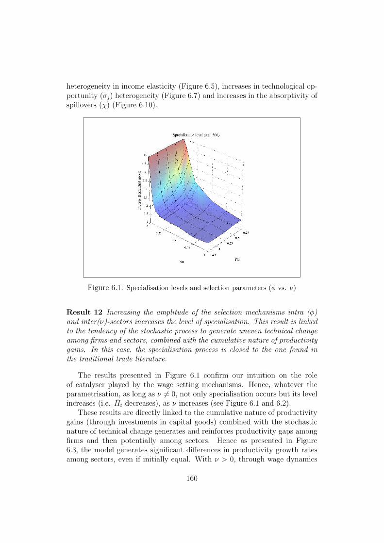
heterogeneity in income elasticity (Figure 6.5), increases in technological op-portunity (σj) heterogeneity (Figure 6.7) and increases in the absorptivity ofspillovers (χ) (Figure 6.10).
Figure 6.1: Specialisation levels and selection parameters (φ vs. ν)
Result 12 Increasing the amplitude of the selection mechanisms intra (φ)and inter(ν)-sectors increases the level of specialisation. This result is linkedto the tendency of the stochastic process to generate uneven technical changeamong firms and sectors, combined with the cumulative nature of productivitygains. In this case, the specialisation process is closed to the one found inthe traditional trade literature.
The results presented in Figure 6.1 confirm our intuition on the roleof catalyser played by the wage setting mechanisms. Hence, whatever theparametrisation, as long as ν 6= 0, not only specialisation occurs but its levelincreases (i.e. Ht decreases), as ν increases (see Figure 6.1 and 6.2).
These results are directly linked to the cumulative nature of productivitygains (through investments in capital goods) combined with the stochasticnature of technical change generates and reinforces productivity gaps amongfirms and then potentially among sectors. Hence as presented in Figure6.3, the model generates significant differences in productivity growth ratesamong sectors, even if initially equal. With ν > 0, through wage dynamics
160
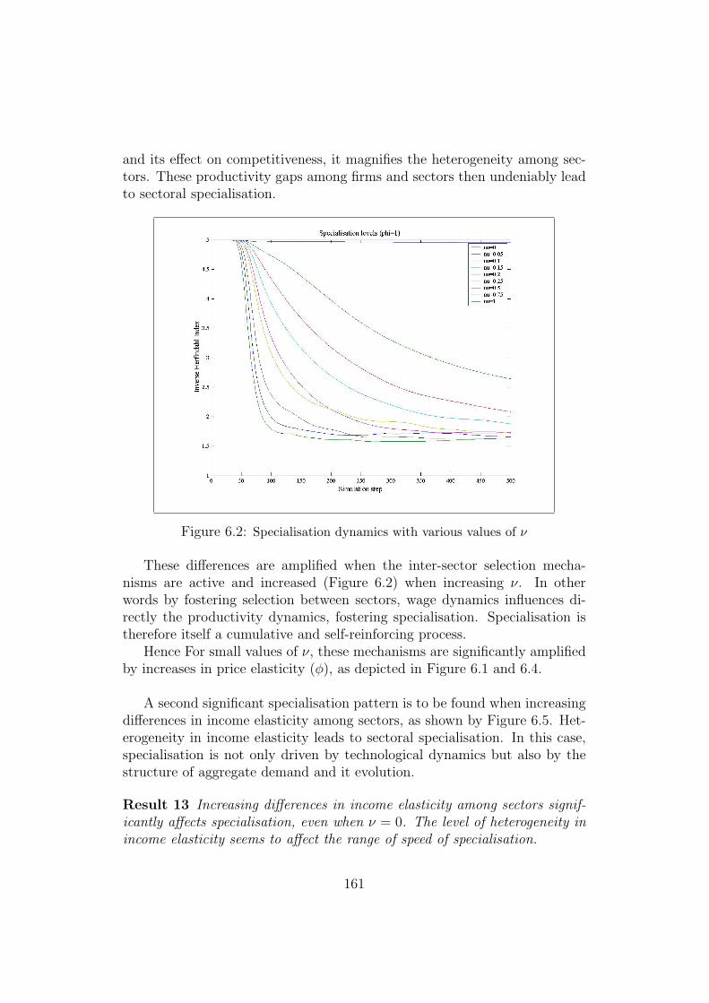
and its effect on competitiveness, it magnifies the heterogeneity among sec-tors. These productivity gaps among firms and sectors then undeniably leadto sectoral specialisation.
Figure 6.2: Specialisation dynamics with various values of ν
These differences are amplified when the inter-sector selection mecha-nisms are active and increased (Figure 6.2) when increasing ν. In otherwords by fostering selection between sectors, wage dynamics influences di-rectly the productivity dynamics, fostering specialisation. Specialisation istherefore itself a cumulative and self-reinforcing process.
Hence For small values of ν, these mechanisms are significantly amplifiedby increases in price elasticity (φ), as depicted in Figure 6.1 and 6.4.
A second significant specialisation pattern is to be found when increasingdifferences in income elasticity among sectors, as shown by Figure 6.5. Het-erogeneity in income elasticity leads to sectoral specialisation. In this case,specialisation is not only driven by technological dynamics but also by thestructure of aggregate demand and it evolution.
Result 13 Increasing differences in income elasticity among sectors signif-icantly affects specialisation, even when ν = 0. The level of heterogeneity inincome elasticity seems to affect the range of speed of specialisation.
161
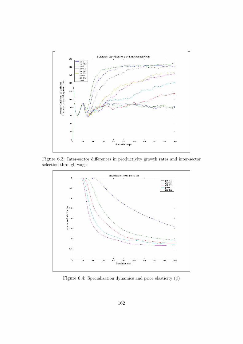
Figure 6.3: Inter-sector differences in productivity growth rates and inter-sectorselection through wages
Figure 6.4: Specialisation dynamics and price elasticity (φ)
162
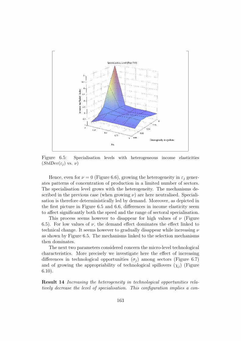
Figure 6.5: Specialisation levels with heterogeneous income elasticities(StdDev(εj) vs. ν)
Hence, even for ν = 0 (Figure 6.6), growing the heterogeneity in εj gener-ates patterns of concentration of production in a limited number of sectors.The specialisation level grows with the heterogeneity. The mechanisms de-scribed in the previous case (when growing ν) are here neutralised. Speciali-sation is therefore deterministically led by demand. Moreover, as depicted inthe first picture in Figure 6.5 and 6.6, differences in income elasticity seemto affect significantly both the speed and the range of sectoral specialisation.
This process seems however to disappear for high values of ν (Figure6.5). For low values of ν, the demand effect dominates the effect linked totechnical change. It seems however to gradually disappear while increasing νas shown by Figure 6.5. The mechanisms linked to the selection mechanismsthen dominates.
The next two parameters considered concern the micro-level technologicalcharacteristics. More precisely we investigate here the effect of increasingdifferences in technological opportunities (σj) among sectors (Figure 6.7)and of growing the appropriability of technological spillovers (χj) (Figure6.10).
Result 14 Increasing the heterogeneity in technological opportunities rela-tively decrease the level of specialisation. This configuration implies a con-
163
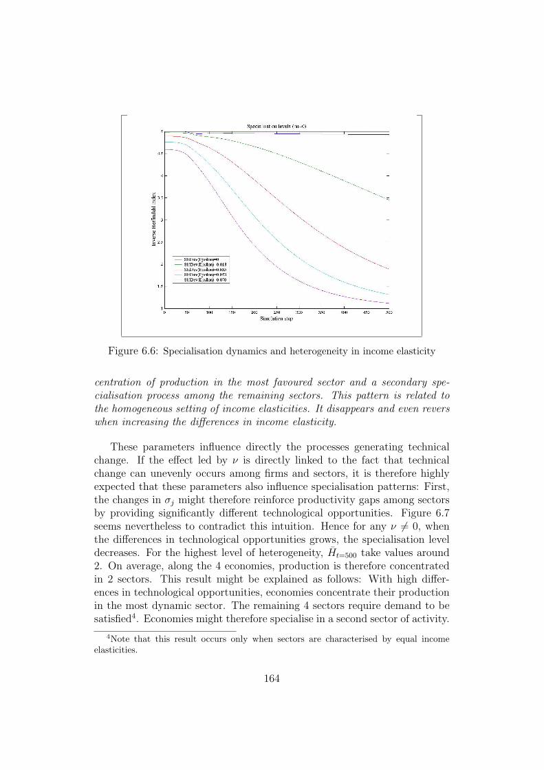
Figure 6.6: Specialisation dynamics and heterogeneity in income elasticity
centration of production in the most favoured sector and a secondary spe-cialisation process among the remaining sectors. This pattern is related tothe homogeneous setting of income elasticities. It disappears and even reverswhen increasing the differences in income elasticity.
These parameters influence directly the processes generating technicalchange. If the effect led by ν is directly linked to the fact that technicalchange can unevenly occurs among firms and sectors, it is therefore highlyexpected that these parameters also influence specialisation patterns: First,the changes in σj might therefore reinforce productivity gaps among sectorsby providing significantly different technological opportunities. Figure 6.7seems nevertheless to contradict this intuition. Hence for any ν 6= 0, whenthe differences in technological opportunities grows, the specialisation leveldecreases. For the highest level of heterogeneity, Ht=500 take values around2. On average, along the 4 economies, production is therefore concentratedin 2 sectors. This result might be explained as follows: With high differ-ences in technological opportunities, economies concentrate their productionin the most dynamic sector. The remaining 4 sectors require demand to besatisfied4. Economies might therefore specialise in a second sector of activity.
4Note that this result occurs only when sectors are characterised by equal incomeelasticities.
164
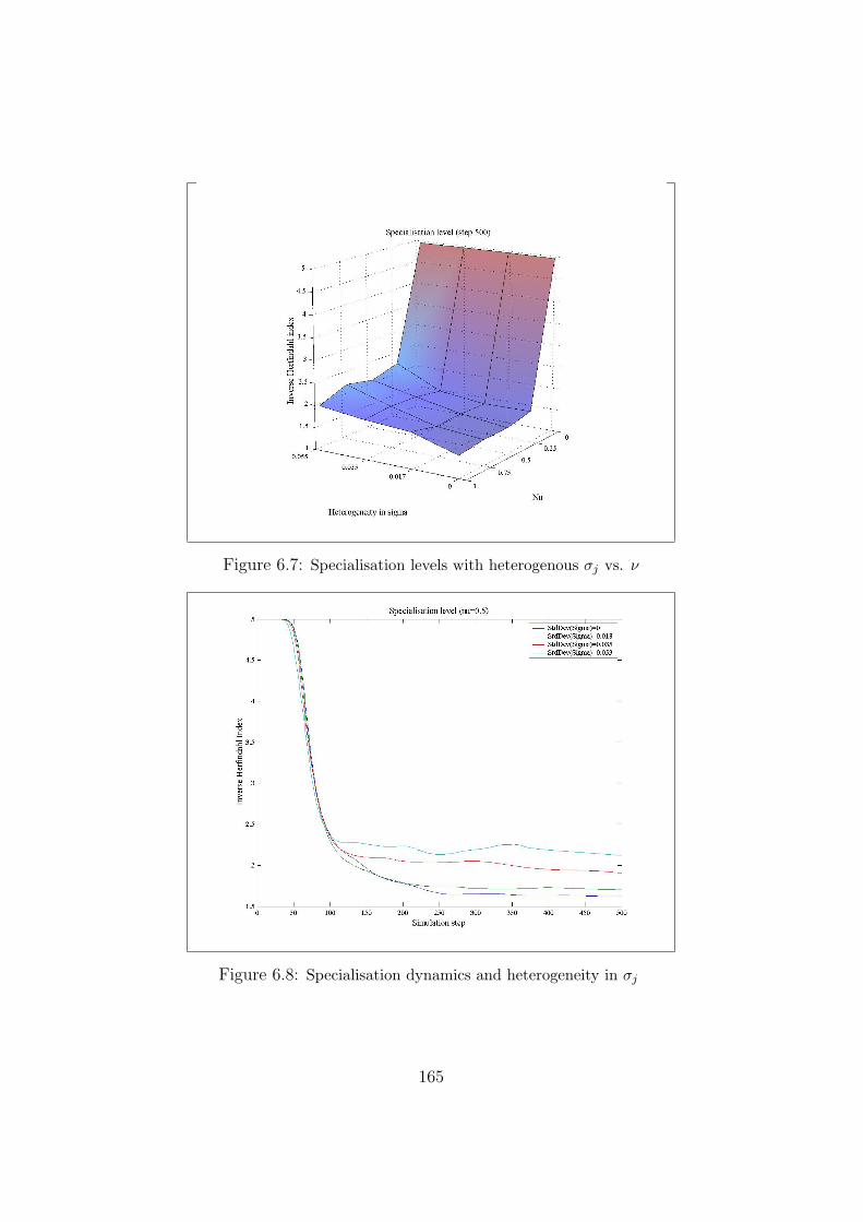
Figure 6.7: Specialisation levels with heterogenous σj vs. ν
Figure 6.8: Specialisation dynamics and heterogeneity in σj
165
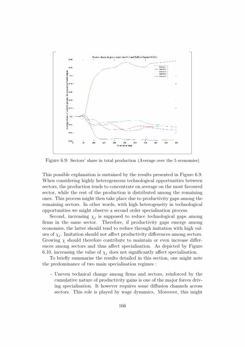
Figure 6.9: Sectors’ share in total production (Average over the 5 economies)
This possible explanation is sustained by the results presented in Figure 6.9.When considering highly heterogeneous technological opportunities betweensectors, the production tends to concentrate on average on the most favouredsector, while the rest of the production is distributed among the remainingones. This process might then take place due to productivity gaps among theremaining sectors. In other words, with high heterogeneity in technologicalopportunities we might observe a second order specialisation process.
Second, increasing χj is supposed to reduce technological gaps amongfirms in the same sector. Therefore, if productivity gaps emerge amongeconomies, the latter should tend to reduce through imitation with high val-ues of χj. Imitation should not affect productivity differences among sectors.Growing χ should therefore contribute to maintain or even increase differ-ences among sectors and thus affect specialisation. As depicted by Figure6.10, increasing the value of χj does not significantly affect specialisation.
To briefly summarise the results detailed in this section, one might notethe predominance of two main specialisation regimes :
- Uneven technical change among firms and sectors, reinforced by thecumulative nature of productivity gains is one of the major forces driv-ing specialisation. It however requires some diffusion channels acrosssectors. This role is played by wage dynamics. Moreover, this might
166
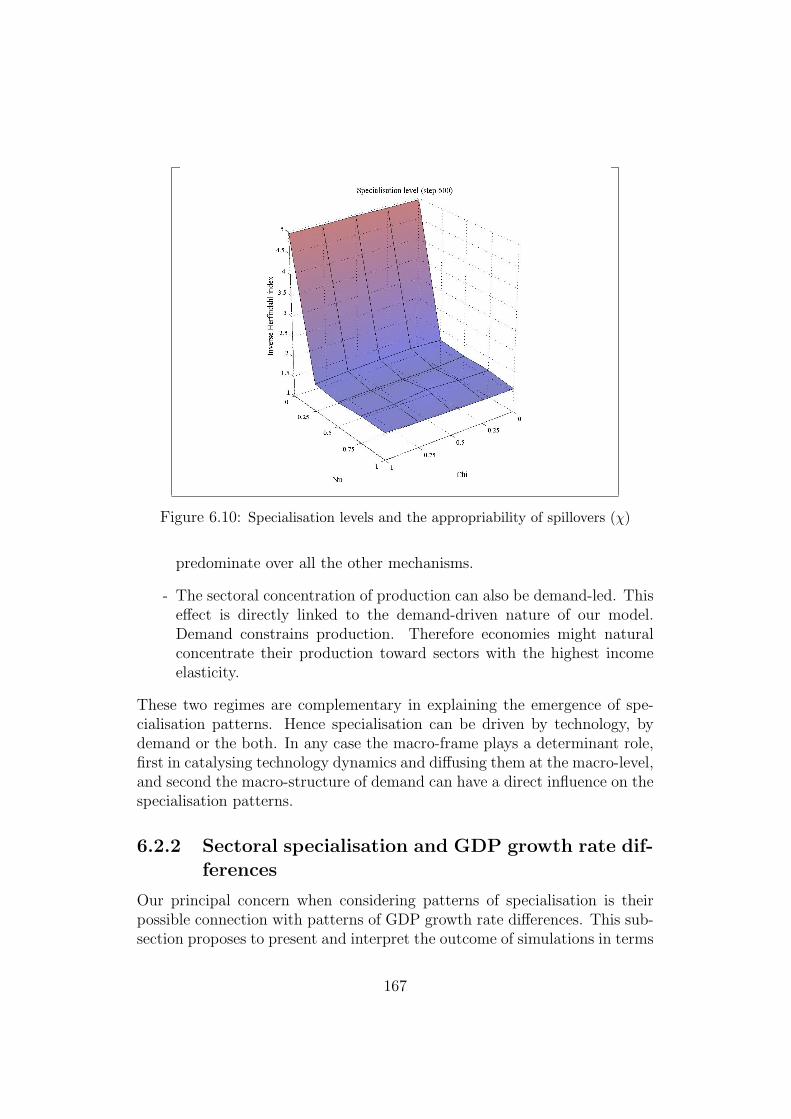
Figure 6.10: Specialisation levels and the appropriability of spillovers (χ)
predominate over all the other mechanisms.
- The sectoral concentration of production can also be demand-led. Thiseffect is directly linked to the demand-driven nature of our model.Demand constrains production. Therefore economies might naturalconcentrate their production toward sectors with the highest incomeelasticity.
These two regimes are complementary in explaining the emergence of spe-cialisation patterns. Hence specialisation can be driven by technology, bydemand or the both. In any case the macro-frame plays a determinant role,first in catalysing technology dynamics and diffusing them at the macro-level,and second the macro-structure of demand can have a direct influence on thespecialisation patterns.
6.2.2 Sectoral specialisation and GDP growth rate dif-ferences
Our principal concern when considering patterns of specialisation is theirpossible connection with patterns of GDP growth rate differences. This sub-section proposes to present and interpret the outcome of simulations in terms
167
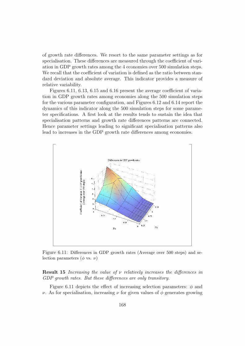
of growth rate differences. We resort to the same parameter settings as forspecialisation. These differences are measured through the coefficient of vari-ation in GDP growth rates among the 4 economies over 500 simulation steps.We recall that the coefficient of variation is defined as the ratio between stan-dard deviation and absolute average. This indicator provides a measure ofrelative variability.
Figures 6.11, 6.13, 6.15 and 6.16 present the average coefficient of varia-tion in GDP growth rates among economies along the 500 simulation stepsfor the various parameter configuration, and Figures 6.12 and 6.14 report thedynamics of this indicator along the 500 simulation steps for some parame-ter specifications. A first look at the results tends to sustain the idea thatspecialisation patterns and growth rate differences patterns are connected.Hence parameter settings leading to significant specialisation patterns alsolead to increases in the GDP growth rate differences among economies.
Figure 6.11: Differences in GDP growth rates (Average over 500 steps) and se-lection parameters (φ vs. ν)
Result 15 Increasing the value of ν relatively increases the differences inGDP growth rates. But these differences are only transitory.
Figure 6.11 depicts the effect of increasing selection parameters: φ andν. As for specialisation, increasing ν for given values of φ generates growing
168
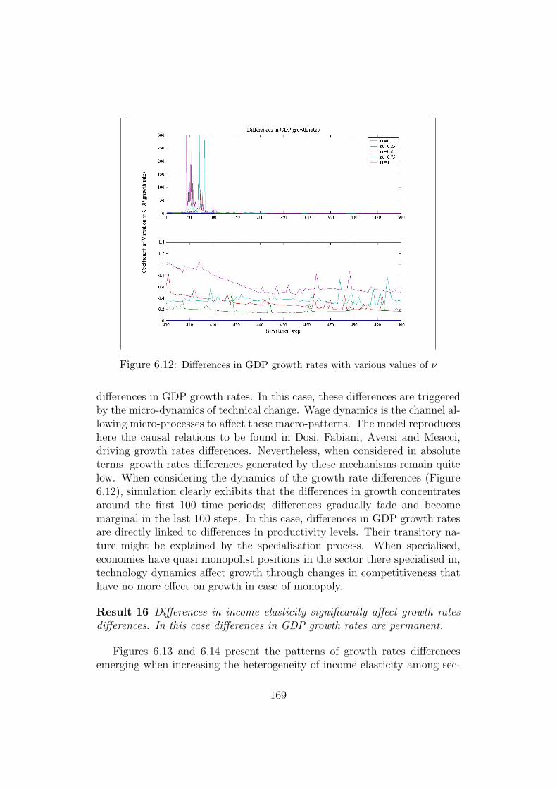
Figure 6.12: Differences in GDP growth rates with various values of ν
differences in GDP growth rates. In this case, these differences are triggeredby the micro-dynamics of technical change. Wage dynamics is the channel al-lowing micro-processes to affect these macro-patterns. The model reproduceshere the causal relations to be found in Dosi, Fabiani, Aversi and Meacci,driving growth rates differences. Nevertheless, when considered in absoluteterms, growth rates differences generated by these mechanisms remain quitelow. When considering the dynamics of the growth rate differences (Figure6.12), simulation clearly exhibits that the differences in growth concentratesaround the first 100 time periods; differences gradually fade and becomemarginal in the last 100 steps. In this case, differences in GDP growth ratesare directly linked to differences in productivity levels. Their transitory na-ture might be explained by the specialisation process. When specialised,economies have quasi monopolist positions in the sector there specialised in,technology dynamics affect growth through changes in competitiveness thathave no more effect on growth in case of monopoly.
Result 16 Differences in income elasticity significantly affect growth ratesdifferences. In this case differences in GDP growth rates are permanent.
Figures 6.13 and 6.14 present the patterns of growth rates differencesemerging when increasing the heterogeneity of income elasticity among sec-
169
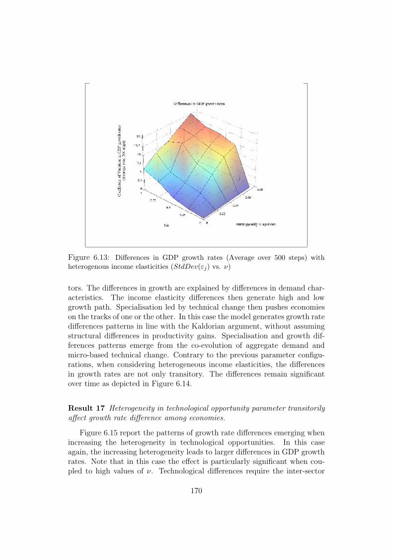
Figure 6.13: Differences in GDP growth rates (Average over 500 steps) withheterogenous income elasticities (StdDev(εj) vs. ν)
tors. The differences in growth are explained by differences in demand char-acteristics. The income elasticity differences then generate high and lowgrowth path. Specialisation led by technical change then pushes economieson the tracks of one or the other. In this case the model generates growth ratedifferences patterns in line with the Kaldorian argument, without assumingstructural differences in productivity gains. Specialisation and growth dif-ferences patterns emerge from the co-evolution of aggregate demand andmicro-based technical change. Contrary to the previous parameter configu-rations, when considering heterogeneous income elasticities, the differencesin growth rates are not only transitory. The differences remain significantover time as depicted in Figure 6.14.
Result 17 Heterogeneity in technological opportunity parameter transitorilyaffect growth rate difference among economies.
Figure 6.15 report the patterns of growth rate differences emerging whenincreasing the heterogeneity in technological opportunities. In this caseagain, the increasing heterogeneity leads to larger differences in GDP growthrates. Note that in this case the effect is particularly significant when cou-pled to high values of ν. Technological differences require the inter-sector
170
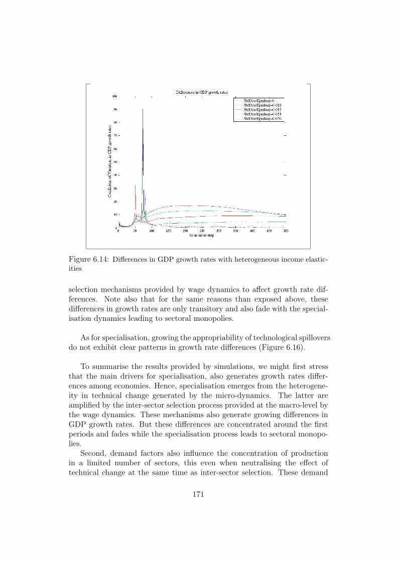
Figure 6.14: Differences in GDP growth rates with heterogeneous income elastic-ities
selection mechanisms provided by wage dynamics to affect growth rate dif-ferences. Note also that for the same reasons than exposed above, thesedifferences in growth rates are only transitory and also fade with the special-isation dynamics leading to sectoral monopolies.
As for specialisation, growing the appropriability of technological spilloversdo not exhibit clear patterns in growth rate differences (Figure 6.16).
To summarise the results provided by simulations, we might first stressthat the main drivers for specialisation, also generates growth rates differ-ences among economies. Hence, specialisation emerges from the heterogene-ity in technical change generated by the micro-dynamics. The latter areamplified by the inter-sector selection process provided at the macro-level bythe wage dynamics. These mechanisms also generate growing differences inGDP growth rates. But these differences are concentrated around the firstperiods and fades while the specialisation process leads to sectoral monopo-lies.
Second, demand factors also influence the concentration of productionin a limited number of sectors, this even when neutralising the effect oftechnical change at the same time as inter-sector selection. These demand
171
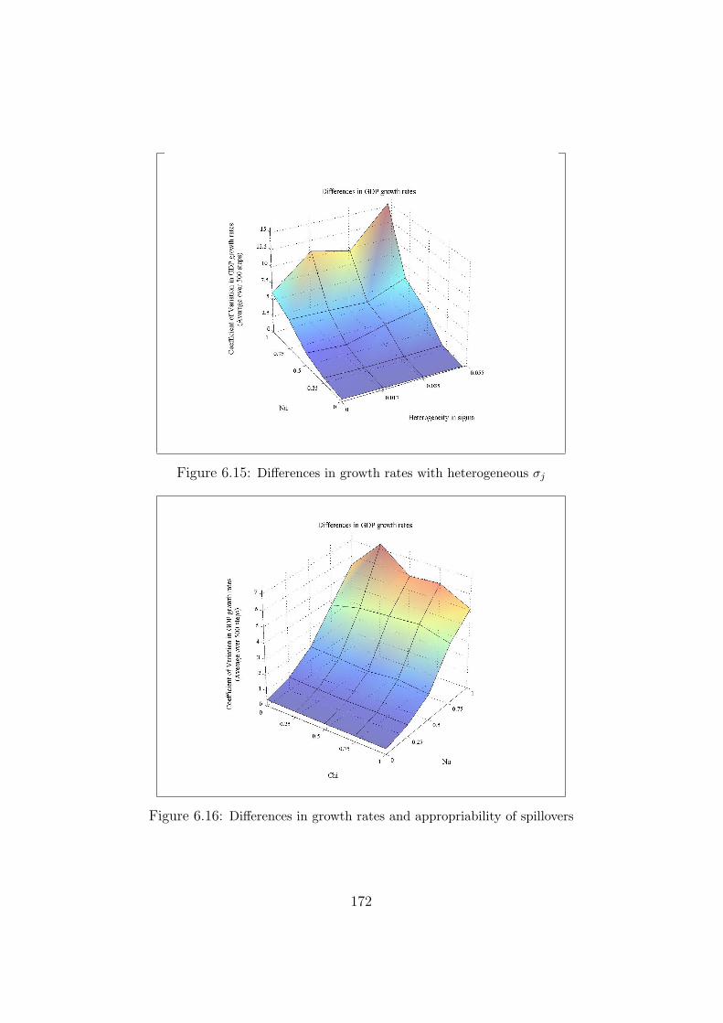
Figure 6.15: Differences in growth rates with heterogeneous σj
Figure 6.16: Differences in growth rates and appropriability of spillovers
172
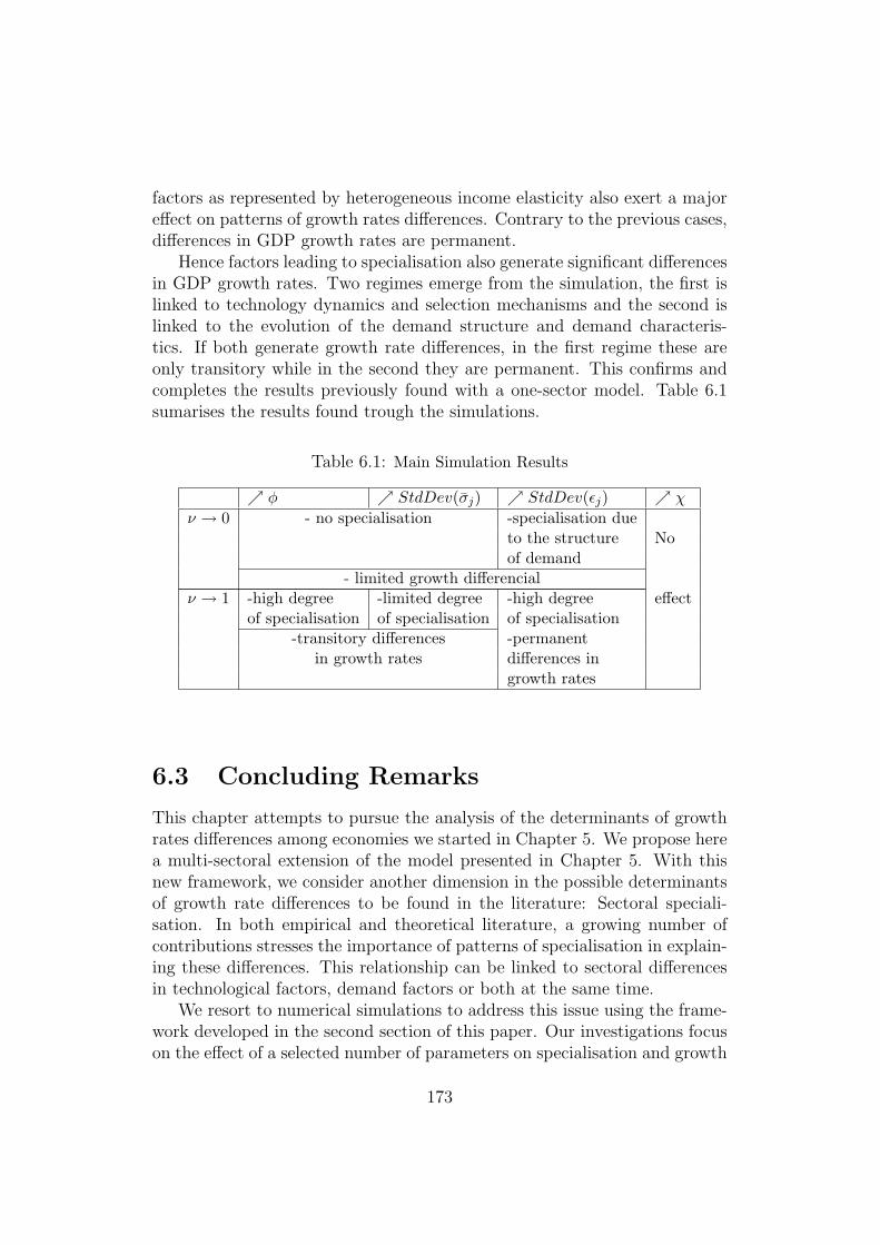
factors as represented by heterogeneous income elasticity also exert a majoreffect on patterns of growth rates differences. Contrary to the previous cases,differences in GDP growth rates are permanent.
Hence factors leading to specialisation also generate significant differencesin GDP growth rates. Two regimes emerge from the simulation, the first islinked to technology dynamics and selection mechanisms and the second islinked to the evolution of the demand structure and demand characteris-tics. If both generate growth rate differences, in the first regime these areonly transitory while in the second they are permanent. This confirms andcompletes the results previously found with a one-sector model. Table 6.1sumarises the results found trough the simulations.
Table 6.1: Main Simulation Results
↗ φ ↗ StdDev(σj) ↗ StdDev(εj) ↗ χ
ν → 0 - no specialisation -specialisation dueto the structure Noof demand
- limited growth differencialν → 1 -high degree -limited degree -high degree effect
of specialisation of specialisation of specialisation-transitory differences -permanent
in growth rates differences ingrowth rates
6.3 Concluding Remarks
This chapter attempts to pursue the analysis of the determinants of growthrates differences among economies we started in Chapter 5. We propose herea multi-sectoral extension of the model presented in Chapter 5. With thisnew framework, we consider another dimension in the possible determinantsof growth rate differences to be found in the literature: Sectoral speciali-sation. In both empirical and theoretical literature, a growing number ofcontributions stresses the importance of patterns of specialisation in explain-ing these differences. This relationship can be linked to sectoral differencesin technological factors, demand factors or both at the same time.
We resort to numerical simulations to address this issue using the frame-work developed in the second section of this paper. Our investigations focuson the effect of a selected number of parameters on specialisation and growth
173
rate differences patterns. Among these parameters, two are related to thedemand factor : price and income elasticity. A third one regulates wagedynamics. The remaining two are linked to technical change.
The results provided by simulation tend to be in line with other existingmodels. These results are only preliminary and require to be confirmed bya deeper analysis of the model. Still they provide already a few interestinginsights.
The main drivers for specialisation, also generates growth rates differencesamong economies. Specialisation emerges from the differences in productivitygains generated by the micro-dynamics, through an inter-sector selectionchannel provided by wage dynamics. In our case, the sources of productivitygrow are not assumed to structurally differ among sectors, as in Verspagen(1993), Cimoli (1994) or Los and Verspagen (2003). In this sense our modelshows that we do not necessary have to assume these structural differencesto observe specialisation patterns.
Simulations also emphasise the influence of demand factors on patternsof concentration of production in a limited number of sectors, this even whenneutralising the effect of technical change at the same time as inter-sectorselection. The influence of the demand structure coupled with the undeniablecatalyser mechanisms played by wage dynamics also stress the importance ofthe macro-frame in diffusing specialisation and growth impulses from microto macro-dynamics.
174

Simulation settings
Table 6.2: Key parameters settings (the values by default are in italic)
Sector 1 Sector 2 Sector 3 Sector 4 Sector 5ν 0 0 0 0 0ν 0.05 0.05 0.05 0.05 0.05ν 0.1 0.1 0.1 0.1 0.1ν 0.15 0.15 0.15 0.15 0.15ν 0.2 0.2 0.2 0.2 0.2ν 0.25 0.25 0.25 0.25 0.25ν 0.5 0.5 0.5 0.5 0.5ν 0.75 0.75 0.75 0.75 0.75ν 1 1 1 1 1φ 0.25 0.25 0.25 0.25 0.25φ 0.5 0.5 0.5 0.5 0.5φ 0.75 0.75 0.75 0.75 0.75φ 1 1 1 1 1φ 1.25 1.25 1.25 1.25 1.25εj 0.2 0.2 0.2 0.2 0.2εj 0.175 0.225 0.2 0.2 0.2εj 0.15 0.25 0.2 0.2 0.2εj 0.125 0.275 0.2 0.2 0.2εj 0.1 0.3 0.2 0.2 0.2σj 0.1 0.1 0.1 0.1 0.1σj 0.075 0.125 0.1 0.1 0.1σj 0.05 0.15 0.1 0.1 0.1σj 0.025 0.175 0.1 0.1 0.1χj 0 0 0 0 0χj 0.25 0.25 0.25 0.25 0.25χj 0.5 0.5 0.5 0.5 0.5χj 0.75 0.75 0.75 0.75 0.75χj 1 1 1 1 1
175
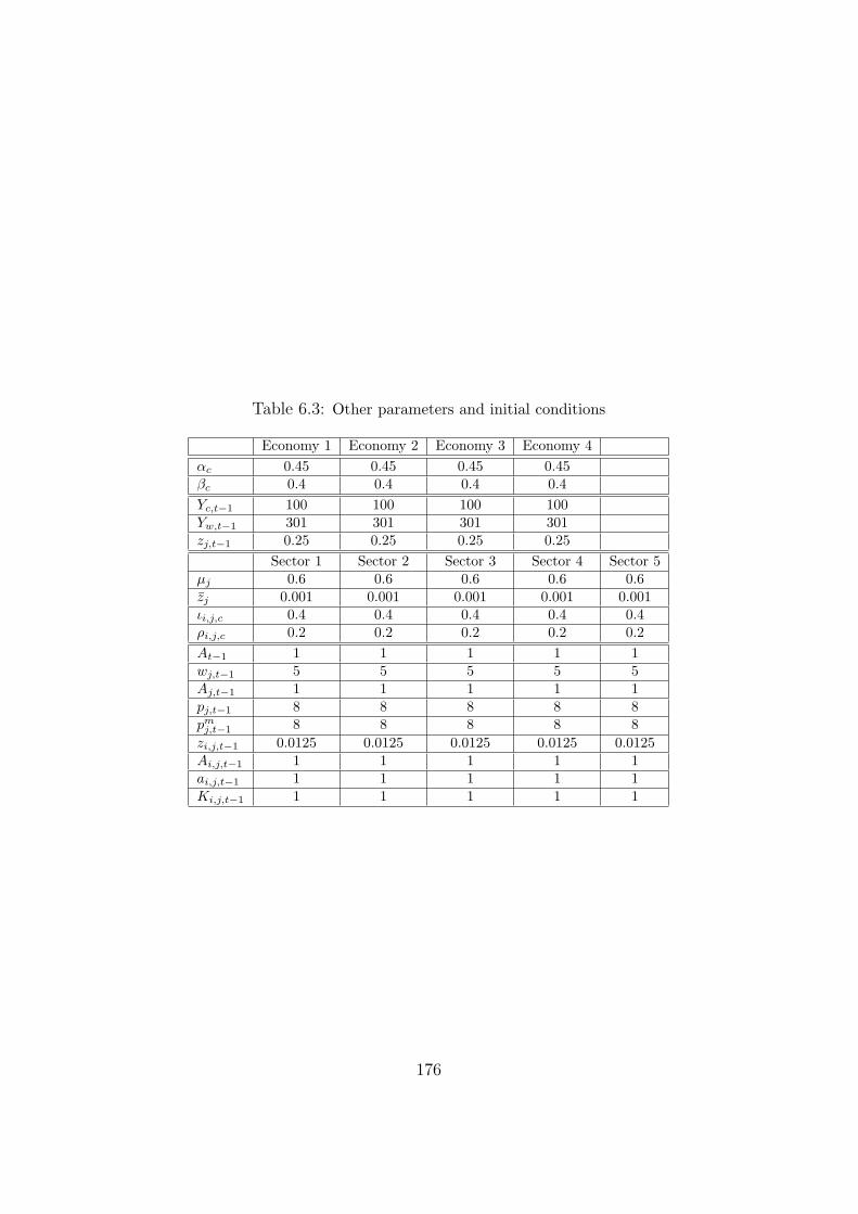
Table 6.3: Other parameters and initial conditions
Economy 1 Economy 2 Economy 3 Economy 4αc 0.45 0.45 0.45 0.45βc 0.4 0.4 0.4 0.4Yc,t−1 100 100 100 100Yw,t−1 301 301 301 301zj,t−1 0.25 0.25 0.25 0.25
Sector 1 Sector 2 Sector 3 Sector 4 Sector 5µj 0.6 0.6 0.6 0.6 0.6zj 0.001 0.001 0.001 0.001 0.001ιi,j,c 0.4 0.4 0.4 0.4 0.4ρi,j,c 0.2 0.2 0.2 0.2 0.2At−1 1 1 1 1 1wj,t−1 5 5 5 5 5Aj,t−1 1 1 1 1 1pj,t−1 8 8 8 8 8pm
j,t−1 8 8 8 8 8zi,j,t−1 0.0125 0.0125 0.0125 0.0125 0.0125Ai,j,t−1 1 1 1 1 1ai,j,t−1 1 1 1 1 1Ki,j,t−1 1 1 1 1 1
176
Chapter 7
Structural Change and GrowthRate Differences
This chapter1 completes the analysis initiated in the previous chapter. Chap-ter 6 has stressed the importance of the composition of aggregate demandin shaping the industrial structure but also the divergence patterns amongeconomies. The structure of aggregate demand is, in the model presentedin the previous chapter, directly induced by the value of income elasticities.These are fixed for every sectors over time. This assumption implies thatfor each sector demand can grow indefinitely, with no satiation level norboundary.
The model presented in this chapter proposes a more elaborated demandstructure. This latter is directly inspired by Pasinetti (1981) and Verspagen(1993). In line with these contributions, we assume that for each sector,demand can reach a ‘satiation’ level or long run share. This long run sharecorresponds to the upper-limit (or satiation) share of income to be devoted toa given sector. Demand dynamics is defined in such a way that in the actualshare of income devoted to a given sector tend to the satiation share in thelong run. The speed of convergence to this limit share then depends on thegrowth rate of income as well as the actual sectoral composition of demandas compared to its long run structure. Moreover we assume that changes insectoral shares are interdependent. Hence the change in the demand share ofa sector does not only depend on its value as compared to the long run valuebut also on the other sectors position with respect to their own long runvalue. In other words changes in sectors can be seen as partially integrated,contrary to the previous chapter’s model in which sectors demand dynamics
1This chapter draws upon a model that has been largely inspired by discussions withB. Verspagen during my stay at ECIS. All usual disclaimer nevertheless apply.
177
were independent. As we below, the assumptions made on the compositionof demand seriously questions some results found previously, especially thoseones on the role played by income elasticities in generating permanent dif-ferences in GDP growth rates. Finally we choose here to release the balanceof payment constraint. This constraint is replaced by the introduction ofexchange rates dynamics, which does not drastically affects or questions ourprevious results.
The chapter is organised as follows: the next section describes the model.Section 7.2 presents and analyses the simulation results.
7.1 A growth model with an evolving demand
structure
This section presents a multi-sectoral growth model with interdependent sec-tors. It considers economic growth as a demand-led process along Kaldorianlines. Contrary to the previous model, GDP growth is not determined bythe balance of payment constraint but is defined by the aggregate internaland external demand. Technical change emerges from the micro-dynamicsfollowing the evolutionary tradition. Despite the release of the balance ofpayment constraint the functioning of the model replicates the one presentedin the previous chapters. Aggregate demand provides the necessary resourcesto finance firms’ technological development and therefore their competitive-ness. Selection among firms and among sectors is rooted in macro-dynamicsthrough demand and wage setting mechanisms. Macro-dynamics generatethe financial resources and are responsible for the mechanisms regulating thedistribution of the latter across firms. In this sense the macro-frame con-straints the micro-dynamics. Micro-dynamics are the core of technologicalchange, and represents one of the engines of growth. The competitiveness ofeconomies, affecting aggregate demand, relies on firms’ ability to gain pro-ductivity.
The structure of the model can be described as follows. We consider a setof C economies integrated in an economic system through trade relations.An economy c ∈ [1; C], is referred to with the index c. The variables indexedc concern foreign economies with regard to the economy c.
Our system counts J sectors of activity. Each economy can produce andconsume products of each sector j ∈ [1; J ].
For each economy, I firms are active in each of the J sectors. A firmi ∈ [1; I], producing in sector j and based in the economy c is referred to
178
with the indexes i, j, c.The entire economic system then counts C economies, J sectors, and
C ∗ J ∗ I firms. The index t refers to the time step.
7.1.1 Macro-constraints: demand dynamics, wages andexchange rates.
Contrary to the models found in the previous chapters, GDP growth is notdetermined by the balance of payment constraint. We choose here to re-lease this constraint. Nevertheless, GDP is still considered as demand con-strained. Hence, we aggregate sectoral demands to define the level of GDP.The computation of aggregate and sectoral demands, as well as the othermacro-components of the model are formally defined as follows.
Aggregate demand:
For each sector j of a given economy c, aggregate demand, in nominal terms,is defined as the sum of two distinct components:
- Domestic consumption (Cj,c,t), defined as a share (sj,c,t−1) of domesticincome equal here to GDP (Yc,t) allocated to the consumption of sectorj products weighted by the market share of the economy in this sector(zj,c,t). Formally, domestic consumption (Cj,c,t) for each sectors arerepresented as follows:
Ci,j,c,t = sj,c,t−1Yc,t−1zj,c,t (7.1)
- Exports in sector j (Xj,c,t) corresponds to the share zj,c,t of the sumof foreign economies imports of sector j products. The latter corre-spond to the share (1 − zj,c,t) of consumption of sector j not coveredby domestic firms. Hence, exports (Xj,c,t) for each sectors are formallydescribed as follows:
Xj,c,t = zj,c,t
∑c
Mj,c,t−1
Xj,c,t = zj,c,t
∑c
ec,t−1sj,c,t−1Yc,t−1(1− zj,c,t) (7.2)
The share of income devoted to the consumption of each sector’s productssj,c,t is defined as follows. We assume here, following Pasinetti (1981) andVerspagen (1993), that sectors dynamics are interrelated. Each sector ischaracterised by an intrinsic or long run share of demand. Every sector
179
tend to this long run share through time, but the evolution of final demandfor every sector is a function of the other sector’s evolution. In this sensewe introduce some degrees of complementarity in the dynamics of sector’sdemand. More formally the share of income sj,c,t devoted to sector j productsgrows proportionally to income growth. As income grows this share tendstowards the long run share sj.
sj,c,t = sj,c,t−1
(1 +
∂sj,c,t
∂Yc,t
∆Yc,t
Yc,t−1
)(7.3)
with
∂sj,c,t
∂Yc,t
= sj,c,t−1
∑j
bjj(sj,c,t−1 − sj)− (sj,c,t−1 − sj)∑j
bjjsj,c,t−1 (7.4)
Hence, the convergence of sj,c,t towards the long run share sj is also functionof the evolution of the other sectors’ shares sj,c,t towards their own long runshares sj. The parameters bjj and bjj capture the degree of interdependencein sectors’ shares evolution. The long run shares sj are defined as follows:
sj =θj∑j θj
Each sector j has an intrinsic value measured by θj. To simplify themodel, θj are exogenous. This value can be explained by institutional orcultural factors. The parameter θj can be subject to exogenous changes. Weintroduce random changes in the long run demand structure of our economiesusing stochastic changes in the value of this parameter (see Section 7.2.2).These changes therefore trigger structural change.
The market share of the economy in a sector is a proxy for the pricecompetitiveness of the economy in the sector. It is given by the sum of themarket shares of the domestic firms active in this sector:
zj,c,t =∑
i
zi,j,c,t
Each firm’s market shares is defined through a replicator dynamic, functionof firm’s relative competitiveness. Hence the market share of each firm willbe computed as follows:
zi,j,c,t = zi,j,c,t−1
(1 + φ
(Ei,j,c,t
Ej,t
− 1
))
180
where zi,j,c,t represents the market share of firm i, pi,j,c,t the price of itsproduct. Ei,j,c,t stands for firm i, in sector j level of competitiveness:
Ei,j,c,t =1
ec,t−1pi,j,c,t
ec,t−1 represents the exchange rate defining the value of the domestic currencyin terms of a foreign reference currency.
Ej,t, the average competitiveness on the international market, is computedas follows:
Ej,t =∑c,i
zi,j,c,t−1Ei,j,c,t
For each sector j the aggregate output (Qj,c,t) is constrained by the levelof demand (Dj,c,t):
Dj,c,t = Qj,c,t ≡∑
i
Qi,j,c,t
The level of demand of sector j corresponds to the sum of domestic and ex-ternal demand. The latter are computed respectively as the level of domesticconsumption (Cj,c,t) deflated by the domestic price level (pj,c,t) and the levelof exports (Xj,c,t) deflated by the domestic price level multiplied by the ex-change rate (ec,t−1pj,c,t). Formally each sector j level of demand2 is thereforedefined as follows:
Dj,c,t =Cj,c,t
pj,c,t
+Xj,c,t
ec,t−1pj,c,t
Dj,c,t =zj,c,t
pj,c,t
[sj,c,t−1Yc,t−1 +
∑c
ec,t−1
ec,t−1
sj,c,t−1Yc,t−1(1− zj,c,t)
](7.5)
At this point we can define the level of GDP of an economy c (Yc,t) innominal terms as follows:
Yc,t =∑j
pj,c,tQj,c,t
Replacing the level of output (Qj,c,t) of each sectors by the expression givenby equation 7.5, we obtain an expression of the GDP level as a function ofthe economies levels of income :
Yc,t =∑j
(sj,c,t−1Yc,tzj,c,t +
zj,c,t
ec,t−1
∑c
ec,t−1sj,c,t−1Yc,t(1− zj,c,t)
)
Yc,t =1
1−∑j sj,c,t−1zj,c,t
∑c
ec,t−1
ec,t−1
Yc,t
∑j
zj,c,tsj,c,t−1(1− zj,c,t) (7.6)
2All the intermediate mathematical computations are provided in the appendix.
181
Trade balance and exchange rate dynamics:
Contrary to the previous chapters we release here two assumptions on thefunctioning of international trades; namely the assumption of fixed exchangerates and the balanced trade assumption. We introduce an explicit exchangerates (ec,t) dynamics. The latter is directly correlated to changes in thetrade balance (Bc,t). Formally exchange rates dynamics is represented bythe following equation:
ec,t = ec,t−1
(1 + β
Bc,t
Yc,t
)(7.7)
The exchange rates dynamics as defined here replicate the idea that tradebalance desequilibria, normalised by GDP (Bc,t
Yc,t) implies capital (or asset)
flows influencing exchange rates. The parameter β catalyses this effects insuch a way that the smaller β is, the more rigid exchange rates are. Con-versely the larger β, the more sensitive to changes in the trade balance theexchange rates are.
Trade balance is logically computed as follows:
Bc,t =∑j
Xj,c,t −∑j
Mj,c,t
Bc,t =∑j
zj,c,t
∑c
sj,c,t−1Yc,t−1 −∑j
(1− zj,c,t)sj,c,t−1Yc,t−1 (7.8)
Wage determination:
Wages are set at the sectoral level. For a given sector j wage dynamics willbe correlated to sector j productivity growth rate ( ∆Aj,c,t
Aj,c,t−1) and to the entire
economy productivity growth rate ( ∆Ac,t
Ac,t−1). The effect of these two variables
on wage dynamics is weighted by the parameter ν ∈ [0; 1], such that :
- When ν = 1, the wage dynamics for every sector only depend on themacro-level productivity growth rate. (i.e. as a centralised wage nego-tiation system)
- When ν = 0, the wage dynamics for every sector only depend on thesector-level productivity growth rate. (i.e. as a decentralised wagenegotiation system)
Wage dynamics of the sector j, in the economy c is represented as follows:
∆wj,c,t
wj,c,t−1
= ν∆Ac,t
Ac,t−1
+ (1− ν)∆Aj,c,t
Aj,c,t−1
(7.9)
182
With
Ac,t =Qc,t
Lc,t
and Aj,c,t =Qj,c,t
Lj,c,t
Note that the wage level defined by this process during the period t is appliedby firms at period t+1. Wage dynamics in our model act as a second macro-constraint on firms. Hence, they affect directly firms competitiveness andthe selection mechanisms on firms. Firms in a given sector will loose com-petitiveness if their own productivity growth rate is slower then the averageone. Moreover, when ν 6= 0, wage dynamics generate a selection processamong sectors. Hence, if the average productivity of a sector grows slowerthen the average productivity growth rate of the entire economy, throughwage dynamics, this sector looses competitiveness. The amplitude of thiseffect directly depends on the value of the parameter ν. As argued in thelast section of this paper wage dynamics through the process described aboveplay a major role in the specialisation dynamics.
7.1.2 Firm level dynamics and the micro-foundationsof technical change: A reminder
This subsection is devoted to the description of the microeconomic function-ing of the model. As for the previous chapter, the micro-dynamics drawlargely on the one presented in Chapter 4.
We consider here the formal representation of firms’ production capaci-ties, investment decisions and R&D activity. Note that the representationprovided applies to all sectors and economies. Sectoral or economy-widespecificity, when considered, take the form of specific parameter values.
The micro-foundations of the model can be summarised as follows. Weconsider a population of bounded rational firms that differ in their technolog-ical characteristics. Technical change emerges at the firm level as a mutationprocess. More precisely technical change is embodied in capital vintagesdeveloped by firms to build and improve their production capacities.
Satisfying demand provides firms with the financial resources to sustainthe development of their production capacities, through investments in cap-ital goods and R&D. This generates technical change.
Defining firms characteristics:
Firms’ production process is represented by a Leontiev production functionwith labour as unique production factor. Capital goods are not used asinput but enter the production function in defining labour productivity. Eachcapital good embodies a level of labour productivity. Hence investment in
183
the different vintages of capital goods modifies the labour productivity of thefirm. The production function is represented as follows :
Qi,j,c,t = Ai,j,c,t−1Li,j,c,t (7.10)
where Qi,j,c,t is the output of firm i, producing in sector j at time t. Ai,j,c,t−1
represents labour productivity and Li,j,c,t the labour force employed in theproduction process. Output is constrained by the demand directed to thefirms and defined at the macro-economic level. The level of production ofeach firm is computed as a share of sector j demand given by their relativemarket share such as:
Qi,j,c,t =zi,j,c,t
zj,c,t
Dj,c,t
Labour productivity is a function of the firms’ accumulation of capitalgoods through investment, so that at the end of any period t :
Ai,j,c,t =Ii,j,c,tai,j,c,t−1∑t
τ=1 Ii,j,c,τ
+
∑t−1τ=1 Ii,j,c,τ∑tτ=1 Ii,j,c,τ
Ai,j,c,t−1 (7.11)
where ai,j,c,t−1 represent the labour productivity embodied in the capital gooddeveloped by the firm i during the period t− 1. Ii,j,c,t represents the level ofinvestment in capital goods of the firm.
Firms set prices through a mark-up process. This mark-up is applied tolabour cost linked to the production process. For the sake of simplicity thelabour costs linked to R&D activity are funded by profits. Prices can thusbe represented as follows:
pi,j,c,t = (1 + µj)wj,c,t−1
Ai,j,c,t−1
(7.12)
where pi,j,c,t represents the price set by firm i at time t, µj the mark-up co-efficient and wj,t−1 the wage level set at the macro level for the entire sector.Note that we assume here that the mark-up coefficients are fixed for eachfirm in a given sector of a given economy.
Firm’s profit level will then be computed as follows:
Πi,j,c,t = pi,j,c,tQi,j,c,t − wj,c,t−1Li,j,t = (1 + µj)wj,c,t−1
Ai,j,c,t−1
Qi,j,c,t − wc,t−1Qi,j,c,t
Ai,j,c,t−1
Πi,j,c,t = µjwj,c,t−1
Ai,j,c,t−1
Qi,j,c,t (7.13)
In the model, profits represent the only financial resource for firms’ invest-ments.
184
Investment decisions and technical change:
As introduced previously, firms have to accumulate capital vintages to buildup and improve their production capacities. Each capital good is developedin-house by firms and then introduced in their production technologies. Thisprocess is decomposed in two phases. First firms explore and develop newcapital goods, through local search or through the adaptation of existingcapital goods to their own production techniques. This phase takes placewithin the R&D activity of the firms. The latter is financed by investmentsin R&D. The second stage consists in introducing the outcome of the R&Dactivity within the production process. This stage is costly and requires firmsto invest in the exploitation of the latest capital good vintage. The level ofinvestment determines the relative importance of the latest capital goodsin the production process and therefore determines the actual productivitygains, as described above. These two distinct investments are subject to thefirms financial constraint. Firms’ only resources for investments are theirprofits. More profitable firms are more inclined to invest and therefore toimprove their production capacities and their competitiveness.
The investment decision timing is set as follows. First firms invest incapital goods, in order to gain from the already developed vintages, andthen invest in R&D.
Investment in capital goods corresponds to a share ιi,j,c of firms’ sales.Given the financial constraint the investment level in capital good is formallyrepresented as follows:
Ii,j,c,t = min {ιi,j,cQi,j,c,t ; Πi,j,c,t} (7.14)
Investments in R&D are a share ρi,j,c of their sales. R&D investment willcorrespond to the hiring of workers assigned to the research activity :
Ri,j,c,t =1
wj,c,t−1
min{ρi,j,cQi,j,c,t; Πi,j,c,t − Ii,j,c,t} (7.15)
The formal representation of the R&D process is explicitly inspired byevolutionary modelling of technical change. Following Nelson and Winter(1982) we consider that the probability of success of research is an increasingfunction of R&D investments. Formally the R&D activity is represented bythe following algorithm:
1. Firms draw a number from a Uniform distribution on [0 ; 1].
2. If this number is contained in the interval [0 ; Ri,j,c,t
Qi,j,c,t], the R&D is
successful. Hence a new capital good vintage has been developed.
185
3. If R&D is successful, its outcome is drawn from the following distri-bution. We differentiate here explicitly innovative firms from imitativeones:
ai,j,c,t = max {ai,j,c,t−1 + εi,j,c,t; ai,j,c,t−1} (7.16)
εi,j,c,t ∼ N(0; σi,j,c,t) (7.17)
with
{σi,j,c,t = σj,c if the firm is an innovatorσi,j,c,t = χj,c(aj,t − ai,j,c,t) if the firm is an imitator
(7.18)
The outcome of the R&D process defines the labour productivity levelembodied in the newly discovered capital vintage (ai,j,c,t). aj,t represents theaverage productivity level embodied in the latest capital vintages developedby firms. It is formally computed as:
aj,t =∑i,c
zi,j,c,tai,j,c,t−1
Hence aj,t−ai,j,c,t represents firm i, j, c technological gap, while the parameterχj,c ∈ [0; 1] can be seen as the degree of access to spillover for the imitatingfirms.
Firms exit the market if their market share is lower then zj. They arereplaced by firms characterised by the average values of the variables for thesector and a market share equal to zj. As a consequence the number of firmsremains constant. An exiting innovator is replaced by an entrant innovator,and an exiting imitator by an entrant imitator. Thus the proportion ofinnovators and imitators remains constant.
7.2 Simulation Results
As for the previous models, we make use of numerical simulations to analysethe dynamics generated by the model. Our aim is to complete the analysisstarted in Chapter 6, on the relation between patterns of specialisation andgrowth rates differences. We therefore choose a similar simulation procedureto conduct the analysis. No ad-hoc assumptions are made on specialisationpatterns nor initial differences in GDP growth rates. All objects composingthe model are set similarly at the initial period. Specialisation patterns aretreated as emergent properties of the model. We therefore aim to isolate thekey mechanisms generating these patterns.
186
Two distinct regimes of specialisation emerged from Chapter 6. First, theuneven nature of technical change among firms and sectors, reinforced by thecumulative nature of productivity gains, leads to the emergence of specialisa-tion patterns when coupled to a catalyser generating an inter-sector selectionmechanism. Wage dynamics play such a role of catalyser (Result 12). Thesecond regime is completely demand-led. Economies concentrate their pro-duction in the sectors with the most dynamic demand growth. These sectorsare characterised by the highest income elasticity (Result 13). In both casesspecialisation led to significant growth rates differences. These differenceswere only transitory if the income elasticities were identical among sectors(Result 17). If sectors were characterised by different levels of income elas-ticities then not only the differences in GDP growth rate became persistent,but the range of the differences was directly shaped by the amplitude of thedifferences in income elasticities (Result 16).
We claim here that the emergence of this second regime and the persis-tence of the growth rates differences are linked to the fixed values of theincome elasticities. We therefore aim to analyse the effect of sectoral het-erogeneity in the ‘satiation’ levels, and of the speed of structural change onspecialisation and growth rates differences. As in the previous chapter thedegree of specialisation of the economies is measured by the average (acrosseconomies) inverse Herfindahl index. Divergence patterns are measured us-ing the coefficient of variation in both real and nominal GDP. The analysisof simulation results is organised as follows. In the next sub-section we con-sider the effect of heterogeneity in satiation level among sectors (i.e. throughthe parameters θj), and speed of convergence of sector’s demand share to-wards their satiation levels (i.e. through the parameters bjj). This effect isanalysed in two cases: in the first case we neutralise the specialisation mech-anisms due to the competition factors. In the second case, these mechanismsare perfectly working. In a second subsection we analyse the effect of demandshocks on the patterns of structural change and growth rates differences, aspreviously found, controlling for the frequency and amplitude of the demandshocks. Again, we differentiate the case in which specialisation mechanismsare neutralised and the one in which this mechanism perfectly work.
Simulations are organised as follows. Our artificial world contains 2economies and 4 industrial sectors. Each economy is producing and con-suming products from each of these sectors. Each sector counts 20 firms,10 from the first economy and the other 10 from the second. Every simula-tion run lasts 1000 periods. We choose in this case longer time periods togenerate structural change. Finally, every simulation setting is replicated 20times. The results presents the average outcome over 20 replications. As forthe previous chapters, all the firms and economies are initially similar. The
187
differences in GDP growth rates as well as in the structure of the economiesare therefore emerging from the dynamics generated by the model.
7.2.1 Demand characteristics and growth rate differ-ences:
We present the results of the simulations when considering the effect ofchanges in demand characteristics in terms of specialisation and growth ratesdifferences patterns. We focus here on two of sectoral demand characteristics:
- Heterogeneity in θ’s; this parameter defines the long run values of sec-tors’ demand share. The degree of heterogeneity of θ therefore definesthe degree of heterogeneity in these long run shares.
- bjj; this parameter controls simultaneously for the degree of inter-sectoral interdependence in the demand shares dynamics, and the speedof convergence of the latter towards their long run values. We assumehere to simplify the analysis that bjj = bjj = b. There are no differencesin terms of interdependence among sectors. The analysis therefore fo-cuses on the speed of convergence towards the long run shares.
We introduce structural differences among sector’s demand through the in-crease in the heterogeneity in θ. This replaces the structural differencesintroduced in the Chapter 6 by the differences in income elasticities. Weanalyse the effect of the changes in these demand parameters consideringtwo specification of the parameter ν.
A first set of simulations results presents the effect of the changes in thedemand parameters on the macro-dynamics when the parameter ν = 0. Inthis case we neutralised the micro-to-macro transmission mechanisms playedby wages. The differences in productivity among sectors are therefore ab-sorbed by wages. We therefore prevent the process of international speciali-sation.
Figure 7.1 presents the effect on the average inverse Herfindahl index after1000 steps of changes in the demand parameters. This index measures thedegree of specialisation of the economies. It estimates the average number ofsectors in which the economies are producing. If increasing the heterogeneityin θ seems to increase specialisation, this influence is however limited. Hence,the index, as shown by Figure 7.1, does not go below 3. In other words, thechanges in demand parameters do not significantly affect the structure ofproduction, contrary to the results found in Chapter 6, when consideringchanges in income elasticities.
188
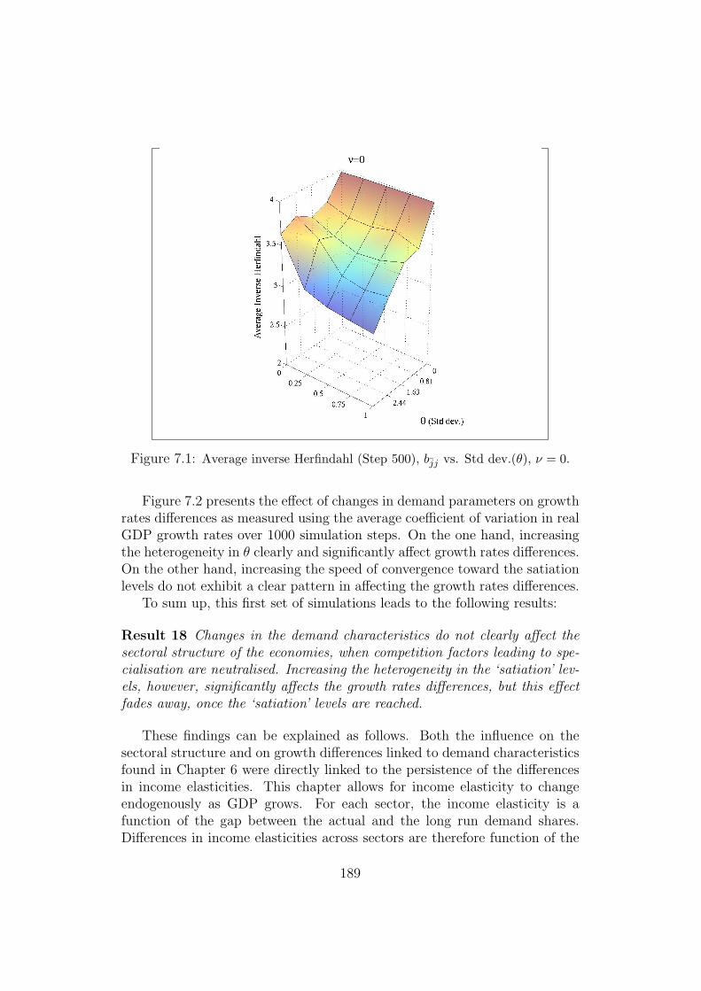
Figure 7.1: Average inverse Herfindahl (Step 500), bjj vs. Std dev.(θ), ν = 0.
Figure 7.2 presents the effect of changes in demand parameters on growthrates differences as measured using the average coefficient of variation in realGDP growth rates over 1000 simulation steps. On the one hand, increasingthe heterogeneity in θ clearly and significantly affect growth rates differences.On the other hand, increasing the speed of convergence toward the satiationlevels do not exhibit a clear pattern in affecting the growth rates differences.
To sum up, this first set of simulations leads to the following results:
Result 18 Changes in the demand characteristics do not clearly affect thesectoral structure of the economies, when competition factors leading to spe-cialisation are neutralised. Increasing the heterogeneity in the ‘satiation’ lev-els, however, significantly affects the growth rates differences, but this effectfades away, once the ‘satiation’ levels are reached.
These findings can be explained as follows. Both the influence on thesectoral structure and on growth differences linked to demand characteristicsfound in Chapter 6 were directly linked to the persistence of the differencesin income elasticities. This chapter allows for income elasticity to changeendogenously as GDP grows. For each sector, the income elasticity is afunction of the gap between the actual and the long run demand shares.Differences in income elasticities across sectors are therefore function of the
189
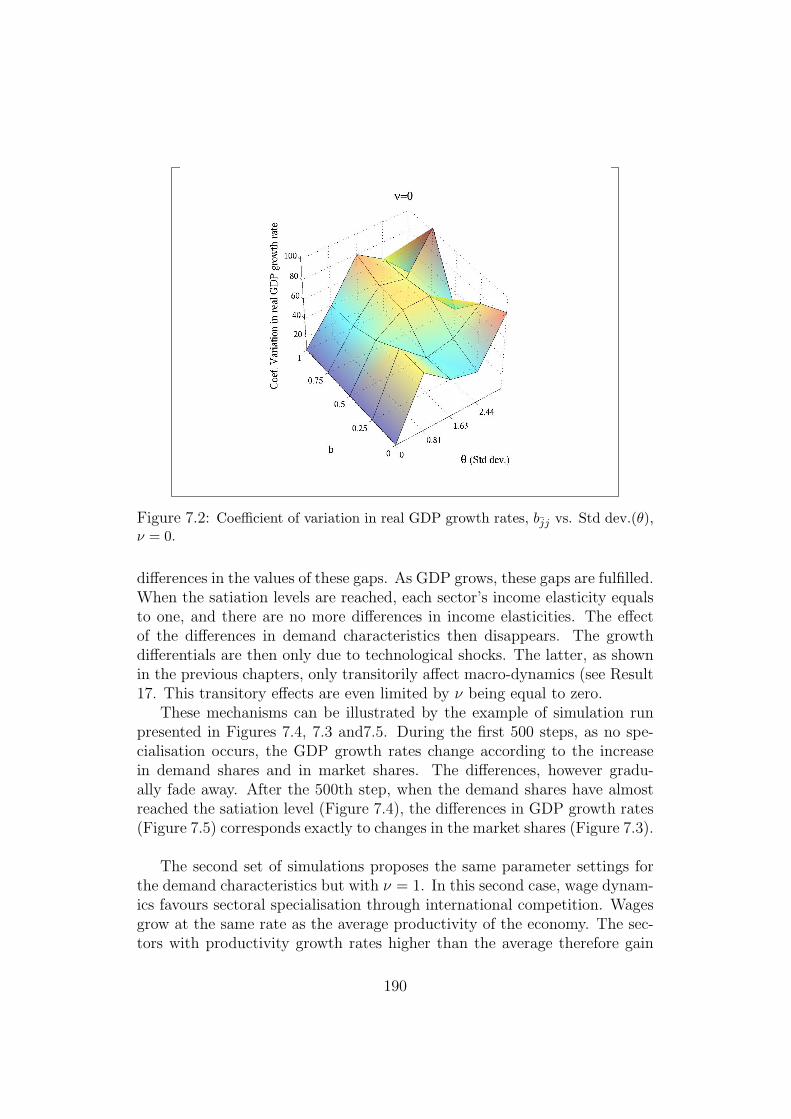
Figure 7.2: Coefficient of variation in real GDP growth rates, bjj vs. Std dev.(θ),ν = 0.
differences in the values of these gaps. As GDP grows, these gaps are fulfilled.When the satiation levels are reached, each sector’s income elasticity equalsto one, and there are no more differences in income elasticities. The effectof the differences in demand characteristics then disappears. The growthdifferentials are then only due to technological shocks. The latter, as shownin the previous chapters, only transitorily affect macro-dynamics (see Result17. This transitory effects are even limited by ν being equal to zero.
These mechanisms can be illustrated by the example of simulation runpresented in Figures 7.4, 7.3 and7.5. During the first 500 steps, as no spe-cialisation occurs, the GDP growth rates change according to the increasein demand shares and in market shares. The differences, however gradu-ally fade away. After the 500th step, when the demand shares have almostreached the satiation level (Figure 7.4), the differences in GDP growth rates(Figure 7.5) corresponds exactly to changes in the market shares (Figure 7.3).
The second set of simulations proposes the same parameter settings forthe demand characteristics but with ν = 1. In this second case, wage dynam-ics favours sectoral specialisation through international competition. Wagesgrow at the same rate as the average productivity of the economy. The sec-tors with productivity growth rates higher than the average therefore gain
190
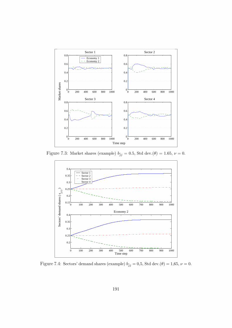
0 200 400 600 800 10000
0.2
0.4
0.6
0.8Sector 1
0 200 400 600 800 10000
0.2
0.4
0.6
0.8Sector 2
0 200 400 600 800 10000
0.2
0.4
0.6
0.8
Time step
Mar
ket s
hare
s
Sector 3
0 200 400 600 800 10000
0.2
0.4
0.6
0.8Sector 4
Economy 1Economy 2
Figure 7.3: Market shares (example) bjj = 0.5, Std dev.(θ) = 1.65, ν = 0.
0 100 200 300 400 500 600 700 800 900 10000.15
0.2
0.25
0.3
0.35
0.4
0 100 200 300 400 500 600 700 800 900 1000
0.2
0.25
0.3
0.35
0.4
Time step
Sect
ors’
dem
and
shar
es (
sj,c
,t )
Economy 2
Sector 1Sector 2Sector 3Sector 4
Figure 7.4: Sectors’ demand shares (example) bjj = 0,5, Std dev.(θ) = 1,65, ν = 0.
191
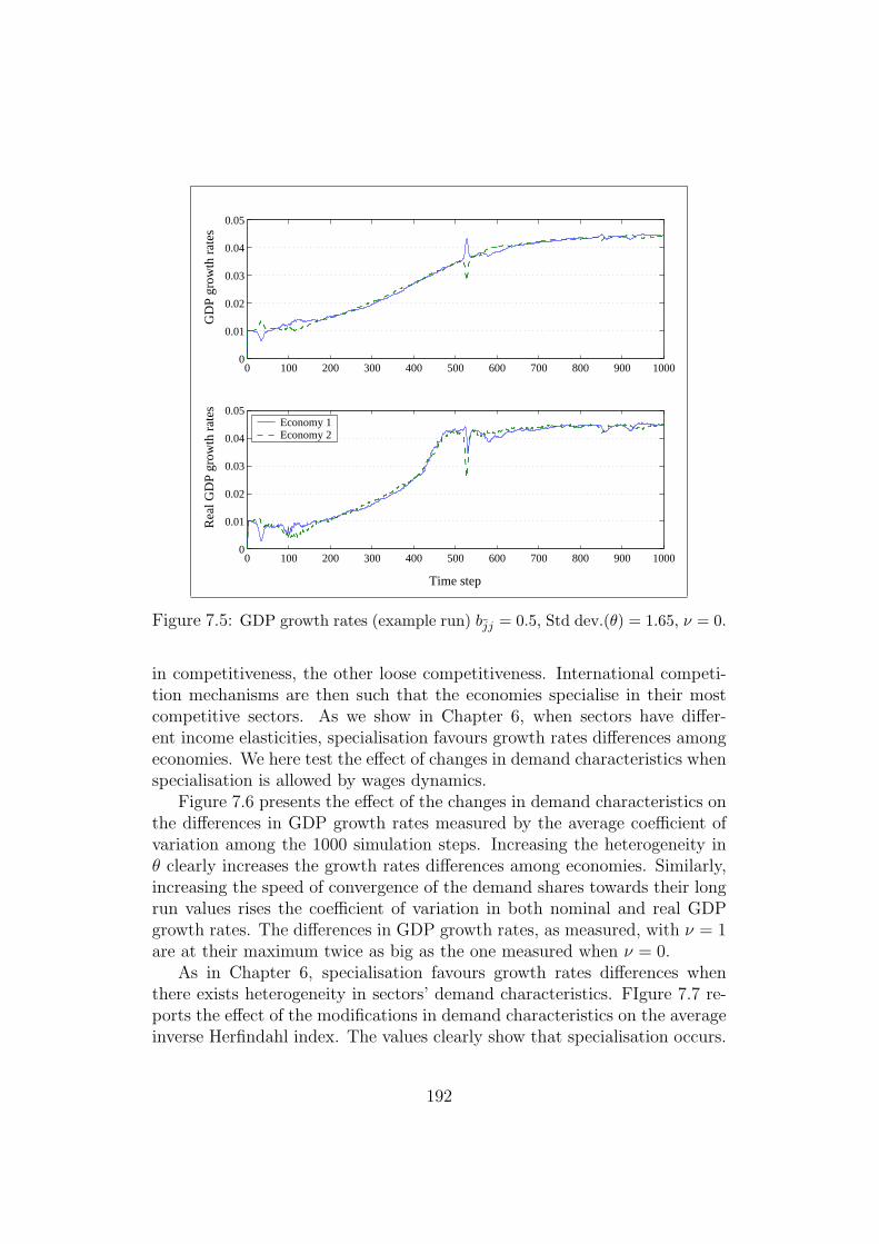
0 100 200 300 400 500 600 700 800 900 10000
0.01
0.02
0.03
0.04
0.05G
DP
grow
th r
ates
0 100 200 300 400 500 600 700 800 900 10000
0.01
0.02
0.03
0.04
0.05
Time step
Rea
l GD
P gr
owth
rat
es
Economy 1Economy 2
Figure 7.5: GDP growth rates (example run) bjj = 0.5, Std dev.(θ) = 1.65, ν = 0.
in competitiveness, the other loose competitiveness. International competi-tion mechanisms are then such that the economies specialise in their mostcompetitive sectors. As we show in Chapter 6, when sectors have differ-ent income elasticities, specialisation favours growth rates differences amongeconomies. We here test the effect of changes in demand characteristics whenspecialisation is allowed by wages dynamics.
Figure 7.6 presents the effect of the changes in demand characteristics onthe differences in GDP growth rates measured by the average coefficient ofvariation among the 1000 simulation steps. Increasing the heterogeneity inθ clearly increases the growth rates differences among economies. Similarly,increasing the speed of convergence of the demand shares towards their longrun values rises the coefficient of variation in both nominal and real GDPgrowth rates. The differences in GDP growth rates, as measured, with ν = 1are at their maximum twice as big as the one measured when ν = 0.
As in Chapter 6, specialisation favours growth rates differences whenthere exists heterogeneity in sectors’ demand characteristics. FIgure 7.7 re-ports the effect of the modifications in demand characteristics on the averageinverse Herfindahl index. The values clearly show that specialisation occurs.
192
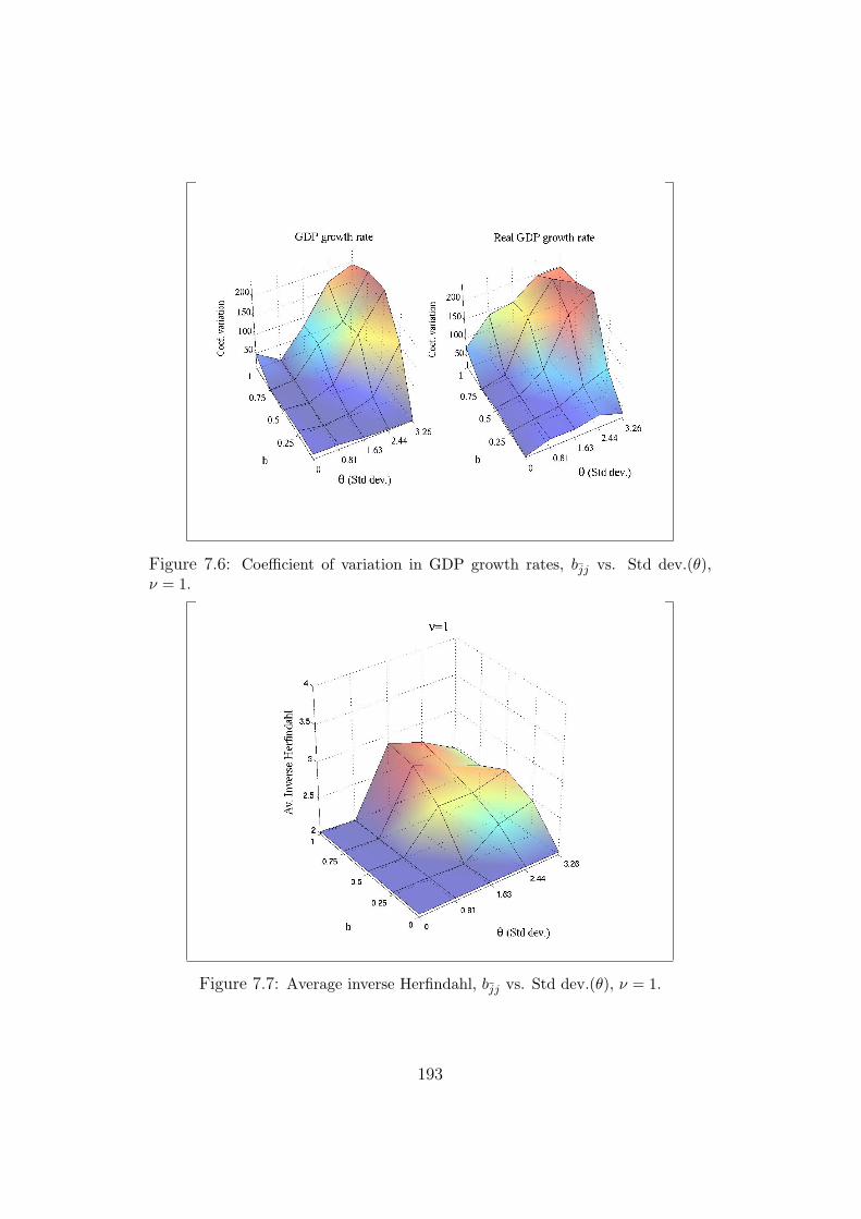
Figure 7.6: Coefficient of variation in GDP growth rates, bjj vs. Std dev.(θ),ν = 1.
Figure 7.7: Average inverse Herfindahl, bjj vs. Std dev.(θ), ν = 1.
193
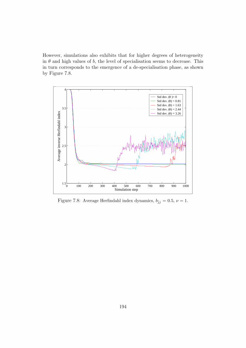
However, simulations also exhibits that for higher degrees of heterogeneityin θ and high values of b, the level of specialisation seems to decrease. Thisin turn corresponds to the emergence of a de-specialisation phase, as shownby Figure 7.8.
0 100 200 300 400 500 600 700 800 900 10001.5
2
2.5
3
3.5
4
Simulation step
Ave
rage
inve
rse
Her
find
ahl i
ndex
Std dev. (θ )= 0Std dev. (θ) = 0.81Std dev. (θ) = 1.63Std dev. (θ) = 2.44Std dev. (θ) = 3.26
Figure 7.8: Average Herfindahl index dynamics, bjj = 0.5, ν = 1.
194
To sum of, this second set of simulations leads to the following results:
Result 19 Specialisation occurs only through market competition channels.When specialisation occurs, the growth differential is significantly higher, ithowever remains transitory. Specialisation is itself transitory. When thegains of specialisation disappear, reaching the satiation levels, economy tendto de-specialise.
These results can be explained as follows. When specialisation occurs,and that sectors have heterogeneous demand characteristics, this leads GDPgrowth rates differences. The economies specialising in the favoured sectorsin terms of demand parameters grow faster than the others. Specialising insectors with the highest demand dynamics implies higher resources availableto invest. These favour the adoption of more efficient production designsby firms, and therefore allows for gains in productivity and competitiveness.These gains reinforces the mechanisms which leads to specialisation. Spe-cialisation is then a self-sustained process.
Due to the changes in the modelling of sectors’ demand and the introduc-tion of ‘satiation’ levels, income elasticities change through time. As GDPgrows, each sector’s income elasticity tends to one, when reaching these ‘sati-ation’ levels. As the gap between the actual and the long run demand sharesreduces, the gains of specialisation (i.e. the resources differentials) graduallydisappear. Specialisation is therefore no more self-reinforced. The emer-gence of technological shocks can then lead to changes in the leadership ofcertain sectors, as well as changes in the competitiveness “hierarchy” amongsectors of the same economy. These two process explains the emergence ofa de-specialisation process. The differences in GDP growth rates are thenonly linked to technological shocks and, as seen in Chapter 6 these are onlytransitory.
These mechanisms can be illustrated by the Figure 7.9, 7.10 and 7.11which present the outcome of an example of simulation run. The parameterssetting used in this example is such that the Sector 1 has the highest long-run share, and Sector 2 the lowest. Specialisation occurs during the first 200steps. Sectors are allocated as follows: Economy 1 specialises in Sector 1and 4. Economy 2 specialises in Sector 2 and 3 (see Figure 7.10). This spe-cialisation pattern clearly affects GDP growth rates (Figure 7.9). Economy2 experiences a lower growth rate. The growth differential gradually reducesuntil the sectors demand reach their long run values between the 500th andthe 600th step (Figure 7.11).
Once the demand stabilises around the satiation levels, the differences inGDP growth rates (Figure 7.9) corresponds exactly to changes in the market
195
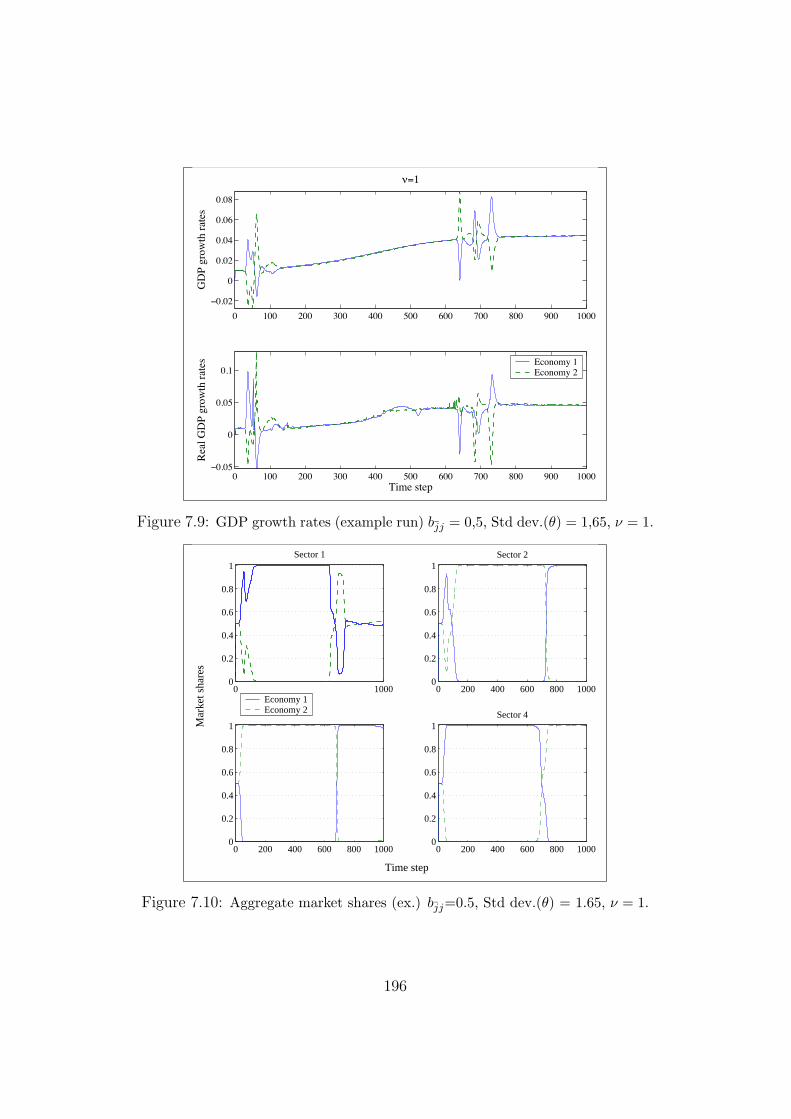
0 100 200 300 400 500 600 700 800 900 1000
−0.02
0
0.02
0.04
0.06
0.08
ν=1
GD
P gr
owth
rat
es
0 100 200 300 400 500 600 700 800 900 1000−0.05
0
0.05
0.1
Time step
Rea
l GD
P gr
owth
rat
es Economy 1Economy 2
Figure 7.9: GDP growth rates (example run) bjj = 0,5, Std dev.(θ) = 1,65, ν = 1.
0 10000
0.2
0.4
0.6
0.8
1
Mar
ket s
hare
s
Sector 1
0 200 400 600 800 10000
0.2
0.4
0.6
0.8
1Sector 2
0 200 400 600 800 10000
0.2
0.4
0.6
0.8
1
0 200 400 600 800 10000
0.2
0.4
0.6
0.8
1
Time step
Sector 4
Economy 1Economy 2
Figure 7.10: Aggregate market shares (ex.) bjj=0.5, Std dev.(θ) = 1.65, ν = 1.
196
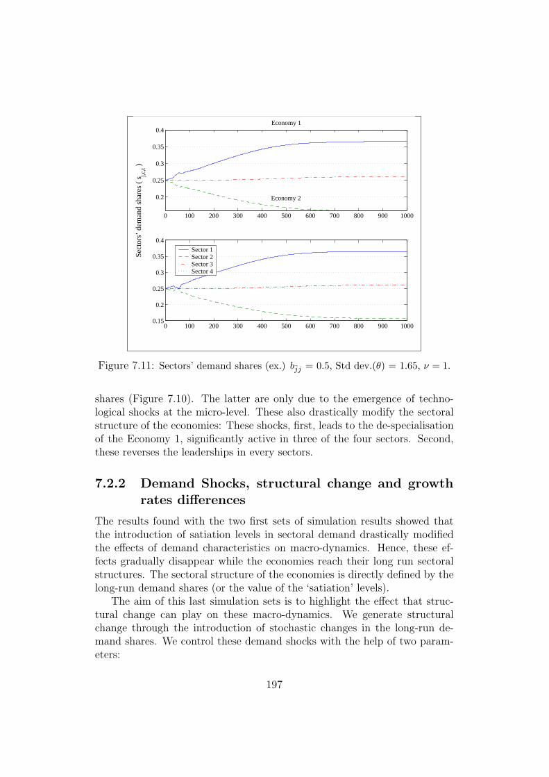
0 100 200 300 400 500 600 700 800 900 1000
0.2
0.25
0.3
0.35
0.4Se
ctor
s’ d
eman
d sh
ares
( s
j,c,t )
Economy 1
0 100 200 300 400 500 600 700 800 900 10000.15
0.2
0.25
0.3
0.35
0.4
Economy 2
Sector 1Sector 2Sector 3Sector 4
Figure 7.11: Sectors’ demand shares (ex.) bjj = 0.5, Std dev.(θ) = 1.65, ν = 1.
shares (Figure 7.10). The latter are only due to the emergence of techno-logical shocks at the micro-level. These also drastically modify the sectoralstructure of the economies: These shocks, first, leads to the de-specialisationof the Economy 1, significantly active in three of the four sectors. Second,these reverses the leaderships in every sectors.
7.2.2 Demand Shocks, structural change and growthrates differences
The results found with the two first sets of simulation results showed thatthe introduction of satiation levels in sectoral demand drastically modifiedthe effects of demand characteristics on macro-dynamics. Hence, these ef-fects gradually disappear while the economies reach their long run sectoralstructures. The sectoral structure of the economies is directly defined by thelong-run demand shares (or the value of the ‘satiation’ levels).
The aim of this last simulation sets is to highlight the effect that struc-tural change can play on these macro-dynamics. We generate structuralchange through the introduction of stochastic changes in the long-run de-mand shares. We control these demand shocks with the help of two param-eters:
197
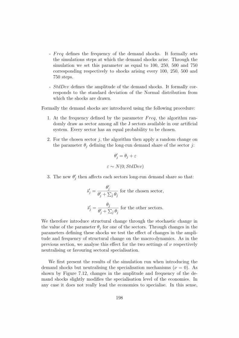
- Freq defines the frequency of the demand shocks. It formally setsthe simulations steps at which the demand shocks arise. Through thesimulation we set this parameter as equal to 100, 250, 500 and 750corresponding respectively to shocks arising every 100, 250, 500 and750 steps.
- StdDev defines the amplitude of the demand shocks. It formally cor-responds to the standard deviation of the Normal distribution fromwhich the shocks are drawn.
Formally the demand shocks are introduced using the following procedure:
1. At the frequency defined by the parameter Freq, the algorithm ran-domly draw as sector among all the J sectors available in our artificialsystem. Every sector has an equal probability to be chosen.
2. For the chosen sector j, the algorithm then apply a random change onthe parameter θj defining the long-run demand share of the sector j:
θ′j = θj + ε
ε ∼ N(0; StdDev)
3. The new θ′j then affects each sectors long-run demand share so that:
s′j =θ′j
θ′j +∑
j θj
for the chosen sector,
s′j =θj
θ′j +∑
j θj
for the other sectors.
We therefore introduce structural change through the stochastic change inthe value of the parameter θj for one of the sectors. Through changes in theparameters defining these shocks we test the effect of changes in the ampli-tude and frequency of structural change on the macro-dynamics. As in theprevious section, we analyse this effect for the two settings of ν respectivelyneutralising or favouring sectoral specialisation.
We first present the results of the simulation run when introducing thedemand shocks but neutralising the specialisation mechanisms (ν = 0). Asshown by Figure 7.12, changes in the amplitude and frequency of the de-mand shocks slightly modifies the specialisation level of the economies. Inany case it does not really lead the economies to specialise. In this sense,
198
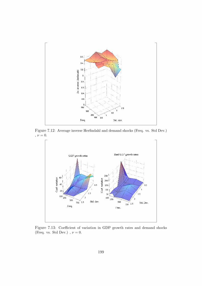
Figure 7.12: Average inverse Herfindahl and demand shocks (Freq. vs. Std Dev.), ν = 0.
Figure 7.13: Coefficient of variation in GDP growth rates and demand shocks(Freq. vs. Std Dev.) , ν = 0.
199

introducing demand shocks does not modify the result previously found onsectoral specialisation (see Result 18).
The introduction of demand shocks affects growth rates differences. Thechanges in the frequency and amplitude of the shocks, however, presents acounterintuitive pattern. In particular, increasing the frequency and ampli-tude of the shocks seems to affect negatively the growth rates differences(Figure 7.13).
This counterintuitive finding con be explained as follows: Specialisationmechanisms are neutralised. The differences in θ, and therefore the demandshocks themselves do not directly affect growth rates differences. Neverthe-less these factors increase the amplitude of the effect of the technologicalshocks on growth differentials. We can then sum-up the results of this thirdset of simulations as follows:
Result 20 When specialisation mechanisms are neutralised, the introduc-tion of demand shocks do not generate growth rates differences. The growthdifferential is due to the micro-level technological shocks. The differencesin demand shares due to the technological shocks shape the amplitude of thedifferences in growth rates consequent to the technological shocks.
0 100 200 300 400 500 600 700 800 900 10000
0.005
0.01
0.015
0.02
GD
P gr
owth
rat
es
0 100 200 300 400 500 600 700 800 900 1000−0.05
0
0.05
Time step
Rea
l GD
P gr
owth
rat
es
�
Economy 1Economy 2
Figure 7.14: GDP growth rates (example run) Freq. = 250, Std dev. = 1, ν = 0.
200
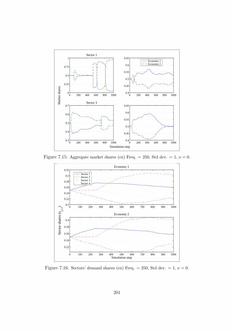
0 200 400 600 800 10000
0.25
0.5
0.75
1M
arke
t sha
res
Sector 1
0 200 400 600 800 10000.4
0.45
0.5
0.55
0.6
0.65
0 200 400 600 800 10000.3
0.4
0.5
0.6
0.7
Simulation step
Sector 3
0 200 400 600 800 10000.4
0.45
0.5
0.55
0.6
0.65�
Economy 1Economy 2
Figure 7.15: Aggregate market shares (ex) Freq. = 250, Std dev. = 1, ν = 0.
0 100 200 300 400 500 600 700 800 900 10000.2
0.22
0.24
0.26
0.28
0.3
0.32Economy 1
0 100 200 300 400 500 600 700 800 900 1000
0.22
0.24
0.26
0.28
0.3
Simulation step
Sect
or s
hare
s (s
j,c,t)
Economy 2
Sector 1Sector 2Sector 3Sector 4
Figure 7.16: Sectors’ demand shares (ex) Freq. = 250, Std dev. = 1, ν = 0.
201
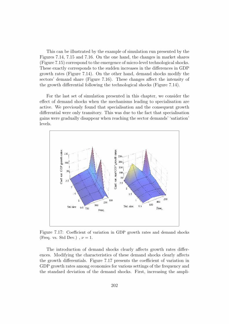
This can be illustrated by the example of simulation run presented by theFigures 7.14, 7.15 and 7.16. On the one hand, the changes in market shares(Figure 7.15) correspond to the emergence of micro-level technological shocks.These exactly corresponds to the sudden increases in the differences in GDPgrowth rates (Figure 7.14). On the other hand, demand shocks modify thesectors’ demand share (Figure 7.16). These changes affect the intensity ofthe growth differential following the technological shocks (Figure 7.14).
For the last set of simulation presented in this chapter, we consider theeffect of demand shocks when the mechanisms leading to specialisation areactive. We previously found that specialisation and the consequent growthdifferential were only transitory. This was due to the fact that specialisationgains were gradually disappear when reaching the sector demands’ ‘satiation’levels.
Figure 7.17: Coefficient of variation in GDP growth rates and demand shocks(Freq. vs. Std Dev.) , ν = 1.
The introduction of demand shocks clearly affects growth rates differ-ences. Modifying the characteristics of these demand shocks clearly affectsthe growth differentials. Figure 7.17 presents the coefficient of variation inGDP growth rates among economies for various settings of the frequency andthe standard deviation of the demand shocks. First, increasing the ampli-
202
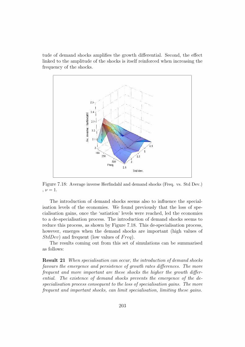
tude of demand shocks amplifies the growth differential. Second, the effectlinked to the amplitude of the shocks is itself reinforced when increasing thefrequency of the shocks.
Figure 7.18: Average inverse Herfindahl and demand shocks (Freq. vs. Std Dev.), ν = 1.
The introduction of demand shocks seems also to influence the special-isation levels of the economies. We found previously that the loss of spe-cialisation gains, once the ‘satiation’ levels were reached, led the economiesto a de-specialisation process. The introduction of demand shocks seems toreduce this process, as shown by Figure 7.18. This de-specialisation process,however, emerges when the demand shocks are important (high values ofStdDev) and frequent (low values of Freq).
The results coming out from this set of simulations can be summarisedas follows:
Result 21 When specialisation can occur, the introduction of demand shocksfavours the emergence and persistence of growth rates differences. The morefrequent and more important are these shocks the higher the growth differ-ential. The existence of demand shocks prevents the emergence of the de-specialisation process consequent to the loss of specialisation gains. The morefrequent and important shocks, can limit specialisation, limiting these gains.
203
These results can be explained as follows: We showed in the previous sec-tion that the introduction of ‘satiation’ levels reduced the impact of special-isation mechanisms on growth differential. The differences in income elas-ticities among sectors disappeared, when the demand shares reached theirlong-run values. This induced the loss of the specialisation gains and of theirimpact on growth differentials.
The introduction of a demand shock mechanically modifies the entiresectoral structure. This restarts the entire income elasticity dynamics whichgenerate new specialisation gains, therefore the self-sustained specialisationprocess and the consequent growth differential.
The amplitude of the shock defines, first, the amplitude of the special-isation gains. The demand shocks re-define the sectoral structure of theeconomy and therefore the differences in demand characteristics among sec-tor. Second, the larger is the amplitude of the shock, the larger the distancebetween the actual and the long-run demand shares. The larger this dis-tance is, the longer the process of structural change. The frequency of thedemand shocks therefore favours the persistence of these structural change.If the demand shocks are too frequent, this can however limits the impactof specialisation. Shocks then arise before the economies fully specialise andgain from this.
The simulation conducted in this chapter highlighted two major results:First, the introduction of ‘satiation’ levels in the sectors demand drasticallymodified the results found in the previous chapter. The demand charac-teristics shape the sectoral structure of the economies. These when com-bined to specialisation explains the emergence of growth differentials. How-ever, the impact of growth rates differences gradually disappear, when theeconomies reach their long run structure. The economies therefore graduallyde-specialise.
Second, the introduction of demand shocks allows for the persistence ofstructural change. The gains of specialisation and its impact on growth ratesdifferences is then favoured by the constancy of structural change. Thisresults is linked to the fact that the mechanisms driving structural changealso preserves the differences in income elasticity among sectors.
Table 7.1 sumarises the results found trough the simulations.
7.3 Concluding remarks
This chapter has aimed to complete the analysis of the determinants ofgrowth rates differences among economies initiated in the two previous chap-
204
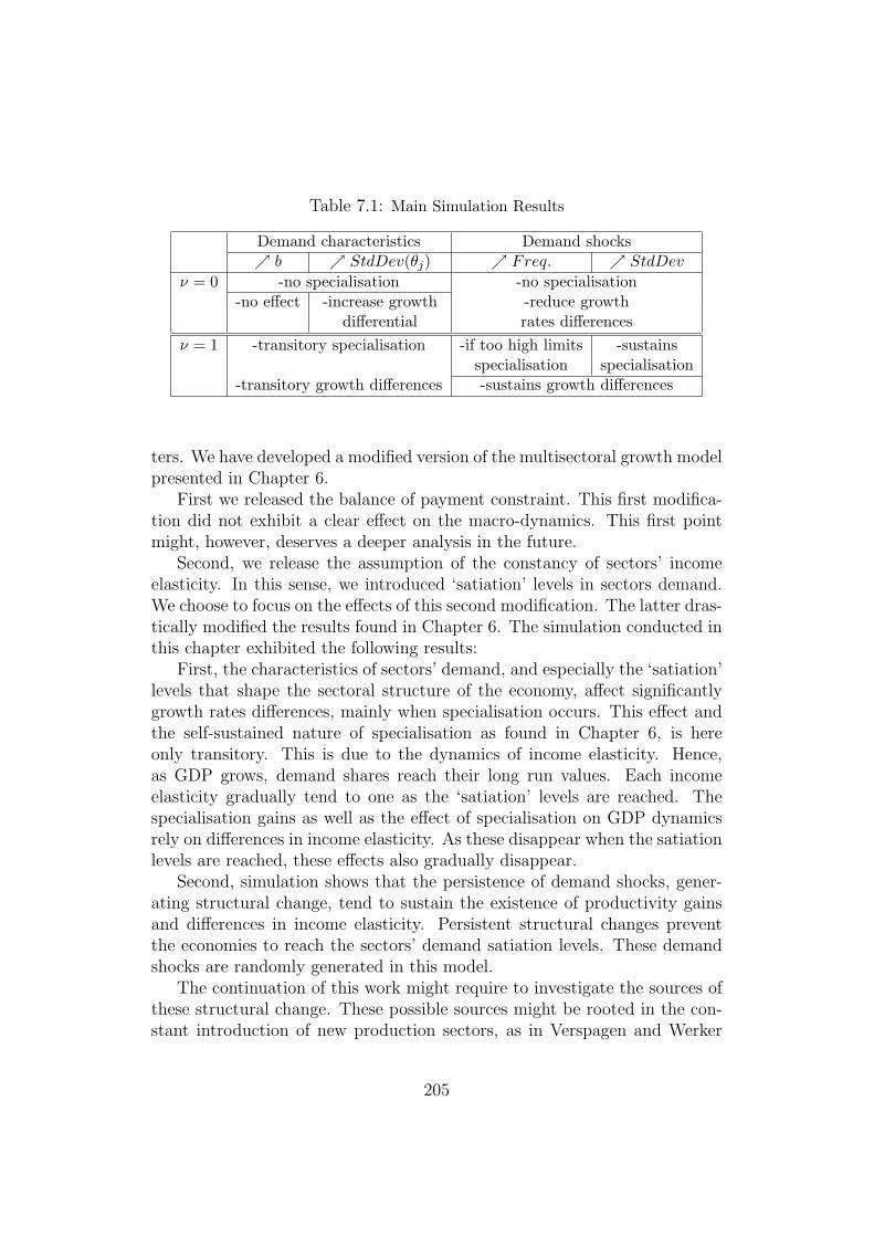
Table 7.1: Main Simulation Results
Demand characteristics Demand shocks↗ b ↗ StdDev(θj) ↗ Freq. ↗ StdDev
ν = 0 -no specialisation -no specialisation-no effect -increase growth -reduce growth
differential rates differencesν = 1 -transitory specialisation -if too high limits -sustains
specialisation specialisation-transitory growth differences -sustains growth differences
ters. We have developed a modified version of the multisectoral growth modelpresented in Chapter 6.
First we released the balance of payment constraint. This first modifica-tion did not exhibit a clear effect on the macro-dynamics. This first pointmight, however, deserves a deeper analysis in the future.
Second, we release the assumption of the constancy of sectors’ incomeelasticity. In this sense, we introduced ‘satiation’ levels in sectors demand.We choose to focus on the effects of this second modification. The latter dras-tically modified the results found in Chapter 6. The simulation conducted inthis chapter exhibited the following results:
First, the characteristics of sectors’ demand, and especially the ‘satiation’levels that shape the sectoral structure of the economy, affect significantlygrowth rates differences, mainly when specialisation occurs. This effect andthe self-sustained nature of specialisation as found in Chapter 6, is hereonly transitory. This is due to the dynamics of income elasticity. Hence,as GDP grows, demand shares reach their long run values. Each incomeelasticity gradually tend to one as the ‘satiation’ levels are reached. Thespecialisation gains as well as the effect of specialisation on GDP dynamicsrely on differences in income elasticity. As these disappear when the satiationlevels are reached, these effects also gradually disappear.
Second, simulation shows that the persistence of demand shocks, gener-ating structural change, tend to sustain the existence of productivity gainsand differences in income elasticity. Persistent structural changes preventthe economies to reach the sectors’ demand satiation levels. These demandshocks are randomly generated in this model.
The continuation of this work might require to investigate the sources ofthese structural change. These possible sources might be rooted in the con-stant introduction of new production sectors, as in Verspagen and Werker
205
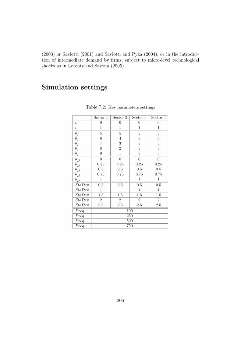
(2003) or Saviotti (2001) and Saviotti and Pyka (2004), or in the introduc-tion of intermediate demand by firms, subject to micro-level technologicalshocks as in Lorentz and Savona (2005).
Simulation settings
Table 7.2: Key parameters settings
Sector 1 Sector 2 Sector 3 Sector 4ν 0 0 0 0ν 1 1 1 1θj 5 5 5 5θj 6 4 5 5θj 7 3 5 5θj 8 2 5 5θj 9 1 5 5bjj 0 0 0 0bjj 0.25 0.25 0.25 0.25bjj 0.5 0.5 0.5 0.5bjj 0.75 0.75 0.75 0.75bjj 1 1 1 1StdDev 0.5 0.5 0.5 0.5StdDev 1 1 1 1StdDev 1.5 1.5 1.5 1.5StdDev 2 2 2 2StdDev 2.5 2.5 2.5 2.5Freq 100Freq 250Freq 500Freq 750
206
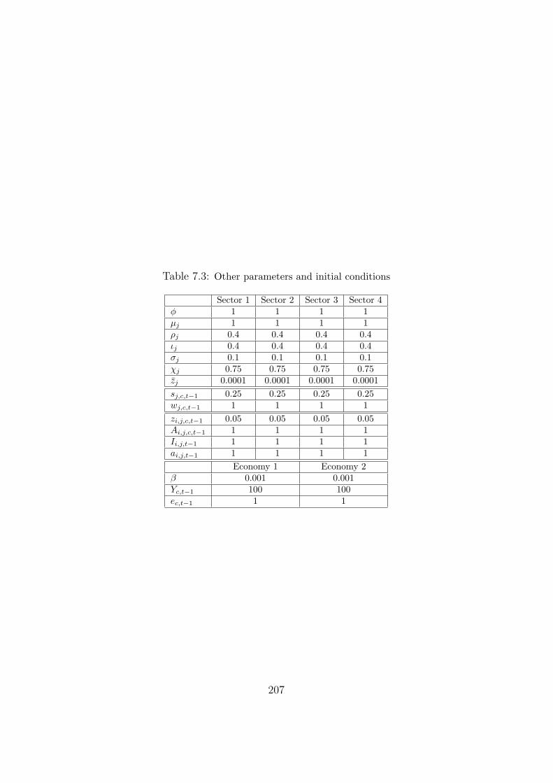
Table 7.3: Other parameters and initial conditions
Sector 1 Sector 2 Sector 3 Sector 4φ 1 1 1 1µj 1 1 1 1ρj 0.4 0.4 0.4 0.4ιj 0.4 0.4 0.4 0.4σj 0.1 0.1 0.1 0.1χj 0.75 0.75 0.75 0.75zj 0.0001 0.0001 0.0001 0.0001sj,c,t−1 0.25 0.25 0.25 0.25wj,c,t−1 1 1 1 1zi,j,c,t−1 0.05 0.05 0.05 0.05Ai,j,c,t−1 1 1 1 1Ii,j,t−1 1 1 1 1ai,j,t−1 1 1 1 1
Economy 1 Economy 2β 0.001 0.001Yc,t−1 100 100ec,t−1 1 1
207

208
Summary of the Results
The aim of this third part was to propose a formal framework for the anal-ysis of the determinants of growth rates differentials. We choose to base theanalysis on the combination of a Post-Keynesian macro-frame inspired by thecumulative causation literature and an evolutionary micro-founded process oftechnological change. We presented three models based on this combination.The mains findings obtained with these models can be summarised as follows.
Chapter 5 presents a baseline one-sector model where the macro-frame isderived from the balance of payment constraint, as in the cumulative causa-tion literature (Dixon and Thirlwall (1975) and Thrilwall (1979)). The micro-dynamics develops around a simple evolutionary representation of technicalchange dynamics at the level of firms. The macro-frame acts as a macro-constraint on the micro-dynamics. The micro-dynamics affect themselvesthe evolution of the macro-frame. The simulation realised with this modelshow the emergence of three distinct regimes:
- The model generates a regime of sustained growth rate differences,which emerges with the introduction of heterogeneity in income elas-ticities. This regime does not necessary imply significant differencesin technologies. The growth rate differential relies on the existenceof differences in income elasticity of exports and/or imports amongeconomies
- The second regime presents transitory phases of divergence. This pat-tern emerges with the introduction of heterogeneity in technologicalopportunities. Its transitory nature is related to the specific settings ofthe wage dynamics. The differences in growth generated by the uneventechnological shocks gradually disappear as the wage dynamics absorbthe uneven technological dynamics.
- The third regime shows a destructive divergence pattern, emergingwhen wage dynamics do not absorb at all technological shocks. In
209
this regime the best firms and economy dominate the market. The lag-ging economies and firms gradually disappear. In this case growth ratedifference increase over time until the collapse of the lagging economies.This regime therefore describes the traditional virtuous vs. vicious cir-cles dichotomy found in the cumulative causation literature.
Chapter 6 presents a multi-sectoral extension to the baseline model. Themacro-frame is again derived from the balance of payment constraint. Themacro-dynamics is here affected by the sectoral structure of the economiesand its changes. The model is used to consider the relationship between spe-cialisation patterns and growth rates differences. The simulations conductedin Chapter 6 show the emergence of two main regimes:
- Uneven technical change among firms and sectors, reinforced by the cu-mulative nature of productivity gains, is one of the major forces drivingspecialisation. These forces also generate differences in GDP growthrates, but these are only transitory. Wages and market dynamics grad-ually absorb the effect of technical change on growth differentials.
- Specialisation mechanisms might lead to permanent growth rates dif-ferences if there exists significant differences in income elasticity amongsectors. These differences in income elasticity generate differences inthe resources available for investments, favouring productivity gainsonly in few sectors. In this case specialisation is self-reinforcing andgrowth rates differentials become permanent.
Chapter 7 slightly modifies the multi-sectoral model developed in Chapter6. We introduced satiation levels to sectors’ demand. These drasticallymodify the outcome of the simulations:
- Specialisation coupled with differences in demand characteristics af-fects directly growth differentials but this effect gradually fades away.In the long run as the economies reach their long-run structure, oncethe sectors’ demand has reached the satiation levels, differences in in-come elasticity disappear. The latter implies that specialisation gainsdisappear.
- Introducing shocks in demand characteristics, we generate structuralchange. The persistence of the shocks prevents the economies to reachthe satiation levels, and therefore growth differences persist.
The main outcome of these models has been to highlight the key roleplayed by the macro-constraints in shaping both macro and technology dy-namics. First, macro-constraints shape macro-dynamics through the dynam-ics of aggregate demand. Second, micro-dynamics requires some catalysers
210

to affect macro-dynamics. This role is mainly played by wages dynamics thatconstitutes one of the macro-constraints.
211

212

Part IV
Conclusions
213

214
Chapter 8
Summary and Conclusions
Understanding why growth rates differ among economies is an age-old issuein economics. The developments of the “New Growth Theory” (NGT), sincethe 90s, brought this issue back at stake in the economic debate. As a mat-ter of fact, NGT has been preceded or contemporary to a long tradition ofresearch, which proposed some alternative explanations to the persistence ofphenomena such as growth rate divergence among countries or regions.
Among these potential alternatives, the Neo-Schumpeterian, or Evolu-tionary approach, considers economic growth as being technology driven.Growth relies on the creation and diffusion of new and more efficient tech-nologies. These technology dynamics are intrinsically uneven and uncertain,but also history dependant. Moreover these are by nature micro-processes.All the macro-dynamics are directly derived from past and present micro-dynamics. Therefore, GDP growth rate differences are directly linked tothe micro-level ability of the economies to generate and/or capture new ormore efficient technologies. Should we then consider that technology explainseverything?
A second alternative to the NGT presents a more embracing answer. ThePost-Keynesian approach also acknowledges the key role played by technol-ogy dynamics. However technical change is seen as a component of a complexset of causal relationships generating economic growth. Kaldor (1966) de-scribes economic growth as being driven by a set of “cumulative causation”.Economic growth is driven by aggregate demand, itself driven by externaldemand fostered by a multiplier effect. External demand is in-turn driven byforeign income and the relative competitiveness of the economy, linked to itstechnology. Therefore, technical change affects growth through the demanddynamics, and is itself linked to the existence of static and dynamic increas-ing returns. These later link the growth of demand to technical change. The
215
combination of these two sets of processes generates the ‘cumulative causa-tion’ mechanisms sustaining growth. Therefore, important macro-feedbacksaffecting technical change are at work and matter for understanding growthrates differences.
Despite the fact that the alternatives to the NGT are usually consideredtoo heterogeneous to be built into an integrated and coherent framework,they actually have some common features, which could justify a comprehen-sive complementarity, as discussed in Chapter 2. In particular, Kaldor’s cu-mulative causation provides Schumpeterians with a more embracing macro-economic framework able to capture the macro-constraints affecting micro-dynamics, while the Evolutionary/Schumpeterian approach provides Kaldo-rians with a micro-founded analysis of the dynamics underlying the processof technological change. We aimed to propose a formal framework integrat-ing these two streams of literature.
The second part of our thesis (Chapters 3 and 4) focused on productivitydynamics and the analysis of increasing returns through the Kaldor-VerdoornLaw. Post-Keynesian and Schumpeterian approaches to growth mechanismsshare above all the idea that technical change, through productivity gainsis one of the key processes generating long-run macro-dynamics. For bothof them technical change relies on the existence of increasing returns, buttheir vision diverge in the formal representation of these increasing returns.This second part aimed to bridge the macro-representation of increasing re-turns proposed by the Kaldorians via the Kaldor-Verdoorn Law to the micro-founded approach proposed by the Schumpeterians.
Chapter 3 proposed to test whether the Law still holds. The use ofthe Kaldor-Verdoorn Law allows us to avoid the abuse of the micro-levelassumptions in the empirical analysis. However, the relevance of the law hasbeen questioned into the literature; first due to the arising of new productionforms, and new sectors of activity after the 70’s crisis; second due to itssensitiveness to the sample of country used.
We first estimated the Law at the macro-economic level using three differ-ent samples of countries: Kaldor (1966) sample of 12 countries, the pre-1974OECD members sample of countries, and a third sample adding to the previ-ous one a selected number of Eastern European, Latin American and SouthEast Asian countries. We used these samples to estimate the Law for fivedecades. When the estimation is restricted to the sample of countries usedby Kaldor (1966), the law does not hold any more after 1970. This result canbe seen as in continuity with the results found by Boyer and Petit (1981) forthe 1970s, supporting their claim that the changes in both production and
216
demand structures led the increasing returns to disappear. Estimated overthe extended samples, the results drastically modify. The law is verified after1980. Two possible explanations can be found to this result. The first in linewith Rowthorn (1975), states that there could be biases due to outliers. Thesecond relies on the division of labour and structural change occurring inthe most advanced economies and which have affected the peripheral ones.Increasing returns being dependent on the structure of the economies, wecould infer that these changes explain that the sources of increasing returnsare from 1970 onwards rather found in the peripheral countries.
In a second phase, we estimated the Kaldor-Verdoorn Law for 56 sec-tors for the two last decades. These estimations show that the law holdssignificantly, for the two periods and the major part of the sectors, includ-ing the non-manufacturing sectors. The empirical results, moreover, showa tendency towards a higher heterogeneity in the levels and significance ofthe estimated parameters of the law for the last period. This heterogeneityis however not linked to the traditional distinction between manufacturingand non-manufacturing sectors as considered by Kaldor (1966). Finally, theestimated values of the parameters of the law at the aggregate level decreasedsignificantly. This latter seems to correspond to changes occurring in a lim-ited number of sectors.
These estimations, however, only provided evidences on the existence ofincreasing returns, at the macro as well as the sectoral level. The use of theKaldor-Verdoorn Law as such does not offer any indications on the sourcesof these increasing returns. Chapter 4 has developed a simple micro-foundedmodel of technological change inspired by the evolutionary literature. We re-verted to this model to identify some sources of the increasing returns. In thisrespect, we analyse the effects of changes in various micro-characteristics ofthe model on the estimates of the Law using the data generated with the sim-ulation model. The simulations showed, first, that a Kaldor-Verdoorn Lawemerges as an aggregated property of these micro dynamics. The analysisalso highlighted that some of the micro-characteristics affect significantly thevalue, significance and robustness of the estimated coefficient of the Law. Onthe one hand, increasing the amplitude of the technological shocks and thestrength of the selection mechanisms, increased the values but decreases thesignificance of the coefficient, and the robustness of the Law. On the otherhand, augmenting the resources devoted to R&D, increasing the frequencyof the shocks, affected positively the value, significance and robustness of theestimated coefficients.
The third part of the thesis (Chapters 5, 6 and 7) presented three for-mal models combining Kaldorian and Evolutionary precepts. Unlike the
217
few existing attempts to be found in the literature (Chapter 2), the modelsdeveloped draw on explicitly evolutionary micro-founded technical changeincluded into a macro-economic framework inspired by the cumulative cau-sation models. The macro-components of the models act on the micro-dynamics as a set of constraints. These macro-constraints are themselvesaffected by the micro-dynamics. In this sense, we included in our modelsa set of feedback mechanisms from macro-to-micro but also from micro-to-macro, around the evolutionary micro-dynamics.
Chapter 5 presented a baseline one-sector model where the macro-frameis derived from the balance of payment constraint, as in the cumulative cau-sation literature (Dixon and Thirlwall (1975) and Thrilwall (1979)). Themicro-dynamics are generated by a simple evolutionary representation oftechnical change dynamics at the level of firms, as developed in Chapter4. The simulation realised with this model showed the emergence of threedistinct regimes: The model generated a regime of sustained growth ratedifferences. The growth rate differential relies on the existence of differencesin income elasticity of exports and/or imports among economies, withoutimplying significant differences in technologies. The second regime presentedtransitory phases of divergence. The differences in growth generated by theuneven technological shocks gradually disappear as the wage dynamics ab-sorb the uneven technological dynamics. The third regime showed a destruc-tive divergence pattern, emerging when wage dynamics do not absorb atall technological shocks. This regime describes the traditional virtuous vs.vicious circles dichotomy found in the cumulative causation literature.
Chapter 6 presented a multi-sectoral extension to the baseline model.The macro-dynamics are affected by the sectoral structure of the economiesand its changes. The chapter considered the relationship between special-isation patterns and growth rates differences. The simulations showed thefollowing results: Uneven technical change among firms and sectors, rein-forced by the cumulative nature of productivity gains, is one of the majorforces driving specialisation. These forces also generate differences in GDPgrowth rates, but these are only transitory. Wages and market dynamicsgradually absorb the effect of technical change on growth differentials. Ifthere exists significant differences in income elasticity among sectors, thesespecialisation mechanisms might lead to permanent growth rates differences.In this case specialisation is self-sustained, generating the resources to fosterits mechanisms, and growth rates differentials become permanent.
Chapter 7 slightly modified the multi-sectoral model, introducing satia-tion levels to sectors’ demand. Again the structure of the economies matteredin the growth process but the changes introduced drastically modify the re-sults of the simulations: Specialisation coupled with differences in demand
218
characteristics affects directly growth differentials but this effect graduallyfades away. In the long run as the economies reach their long-run structure,once the sectors’ demand has reached the satiation levels, differences in in-come elasticity disappear, then specialisation gains disappear. Introducingshocks in demand characteristics, we generate structural change. The persis-tence of the shocks prevents the economies to reach the satiation levels, andtherefore growth differences persist.
Reverting to these models has highlighted the key role played by themacro-constraints in shaping both macro and technology dynamics. Firstthe aggregate demand dynamics constraints growth and growth differen-tials. This affects the resources allocated to investments and therefore affectstechnical change. There exists therefore an important macro-to-micro feed-back mechanism. Second, micro-dynamics relies on two macro-mechanisms,namely market selection and wage dynamics to affect growth and the growthdifferential. Macro-constraints are therefore required for the functioning ofthe micro-to-macro feedback.
Moreover, contrary to the Harrod-Domar framework, our framework doesnot oppose demand and technology dynamics in shaping the growth process.These two components rather appear complementary in defining the growthmechanisms and explaining growth differentials among economies. Alongthe simulations, demand dynamics appeared as defining the broad macroand meso growth trends and their changes. Technology dynamics on theother side defines rather the fluctuations and specialisation patterns withinthis broad growth trends. Hence, via the selection mechanisms, technologydynamics helps the allocation among firms and economies of the resourcesprovided by the extension of demand.
Understanding why growth rates differ among economies, requires there-fore not only to account for demand or technological determinants, but totake also into account the whole set of feedback mechanisms that links thesedeterminants. In our framework these mechanisms are mainly found amongthe macro-constraints. Among these, wage dynamics, selection mechanismsand/or the structure of the aggregate demand and its changes play crucialrole in understanding the growth differential. These factors, however remain,unexplained in our models, opening a wide potential for future developments.We might more particularly stress the micro-foundations of the labour mar-ket mechanisms underlying the wage dynamics, the micro-foundations of de-mand dynamics defining the structure and the changes in the structure offinal and intermediate demand or the market mechanisms underlying theselection mechanisms.
219

220

Bibliography
[1] M. Abramovitz (1989) Thinking About Growth, and other Essays onEconomic Growth and Welfare. Cambridge University Press.
[2] P. Aghion and P. Howitt (1992) A Model of Growth Through CreativeDestruction. Econometrica, 60(2):323–35.
[3] B. Amable (1992) Effets d’apprentissage, competitivite hors-prix etcroissance cumulative. Economie Appliquee.
[4] B. Amable (1993) Catch-up and Convergence: A Model of CumulativeGrowth. International Review of Applied Economics.
[5] M. Amendola and J.L. Gaffard (1998) Out of Equilibrium. ClarendonPress, Oxford.
[6] E. S. Andersen (1994) Evolutionary Economics: Post Schumpeteriancontributions. Pinter Publishers, London and New York.
[7] J. Arrous (1987) Analyse multisectorielle et croissance. Economica,Paris.
[8] J. Arrous (1999) Les Theories de la croissance. Editions du Seuil,Paris.
[9] R.J. Barro (1990) Government Spending in a Simple Model of Endoge-nous Growth. Journal of Political Economy, 5(98):S103–S125.
[10] R. Boyer and M. Juillard (1992) The New Endogenous Growth The-ory versus a Productivity Regime Apporach. Document de travail,CEPREMAP, Paris.
[11] R. Boyer and P. Petit (1981) Productivite dans l’industrie et croissancea moyen terme. Document de travail, CEPREMAP, Paris.
221
[12] R. Boyer and P. Petit (1991) Kaldors Growth Theories: Past, Presentand Prospects for the Future. E.J. Nell and W. Semmler (eds).
[13] M.J.C. Caniels and B. Verspagen (1999) Spatial Distance in a Tech-nology Gap Model. Technical report, ECIS Working Paper.
[14] C. Castaldi (2002) An Evolutionary Model of International Competi-tion and Growth. Working paper, LEM, Sant’Anna School, Pisa.
[15] C. Castaldi (2003) Essays On The Process Of Economic Growth. Un-published PhD dissertation, Sant’Anna School For Advanced Studies.
[16] C. Castaldi and G. Dosi (2003) The Grip of History and the Scope forNovelty. Working Paper 2003-02, LEM, Sant’Anna School, Pisa.
[17] F. Castellacci (2001) Technology Gap and Cumulative Causation:Models, Results and Performances. In ETIC Conference 2001 Pro-ceedings.
[18] F. Castellacci (2001) A ‘Technology-Gap Approach to CumulativeGrowth’: Towards an Integrated Model. Empirical Evidence for Spain,1960-1997. Technical report, DRUID Working Paper, Aalborg.
[19] F. Chiaromonte and G. Dosi (1993) Heterogeneity, Competition andMacroeconomic Dynamics. Structural Change and Economic Dynam-ics.
[20] M. Cimoli (1988) Technological Gaps and Institutional Asymmetriesin a North-South Model with a Continuum of Goods. Metroeconomica.
[21] M. Cimoli (1994) Lock-in and Specialization (Dis) Advantages in aStructuralist Growth Model. in J. Fagerberg, B. Verspagen and N.Von Tunzelmann (eds.).
[22] M. Cimoli and G. Dosi (1995) Technological Paradigms, Patterns ofLearning and Development: An Introductory Roadmap. Journal ofEvolutionary Economics, 5:243–268.
[23] M. Cimoli, G. Dosi, and L. Soete (1986) Innovation Diffusion Institu-tional Differences and Patterns of Trade: A North-South Model. Drcpaper n. 36, SPRU, University of Sussex.
[24] J.S.L. Mc Combie and A.P. Thirlwall (1994) Economic Growth and theBalance of Payments Constraint. MacMillan Press.
222
[25] B. Dalum, K. Laursen, and B. Verspagen (1999) “Does SpecializationMatter for Growth?”. Industrial and Corporate Change.
[26] R. Dixon and A.P. Thirlwall (1975) A Model of Regional Growth-RateDifferences on Kaldorian Lines. Oxford Economic Papers.
[27] E.D. Domar (1946) Capital Expansion, Rate of Growth and Employ-ment. Econometrica, 14:137–147.
[28] G. Dosi and C. Castaldi (2002) Local and Divergent Patterns of Tech-nological Learning within (Partly) Globalized Markets. Working Paper2002-22, LEM, Sant’Anna School, Pisa.
[29] G. Dosi and S. Fabiani (1994) Convergence and Divergence in theLong-Term Growth of Open Economies. in G. Silverberg and L. Soete(eds.).
[30] G. Dosi, S. Fabiani, R. Aversi, and M. Meacci (1994) The Dynamicsof International Differentiation: A Multi-Country Evolutionary Model.Industrial and Corporate Change.
[31] G. Dosi, C. Freeman, and S. Fabiani (1994) The Process of EconomicDevelopment: Introducing Some Stylised Facts and Theories on Tech-nologies, Firms and Institutions. Industrial and Corporate Change.
[32] G. Dosi, C. Freeman, R. Nelson, G. Silverberg, and L. Soete (1988)Technical Change and Economic Activity. Pinter.
[33] G. Dosi, K. Pavitt, and L. Soete (1990) The Economics of TechnicalChange and International Trade. Harvester Wheatsheaf, London.
[34] K. Dopfer (1996) The Global Dimension of Economic Evolution:Knowledge Variety and Diffusion in Economic Growth and Develop-ment. Physica-Verlag, Heidelberg.
[35] J. Fagerberg (1987) A Technology Gap Approach to Why Growth RateDiffer. Research Policy.
[36] J. Fagerberg (2000) Technological Progress, Structural Change andProductivity Growth: A Comparative Study. Structural Change andEconomic Dynamics.
[37] J. Fagerberg, P. Guerrieri, and B. Verspagen (1999) The EconomicChallenge for Europe: Adapting to Innovation Based growth. E.Elgar.
223
[38] J. Fagerberg and B. Verspagen (1996) Heading for Divergence? Re-gional Growth in Europe Reconsidered. Journal of Common MarketStudies.
[39] J. Fagerberg and B. Verspagen (2001) Technology-Gaps, Innovation-Diffusion and Transformation: An Evolutionary Interpretation. Work-ing paper, ECIS, Eindhoven.
[40] J. Fagerberg, B. Verspagen, and N. Von Tunzelmann (1994) The Dy-namics of Technology, Trade and Growth. E.Elgar.
[41] B. Fine (2000) Endogenous Growth Theory: A Critical Assessment.Cambridge Journal of Economics, 24:pp.245–265.
[42] C. Freeman and L. Soete (1997) The Economics of Industrial Innova-tion, 3rd edition. Pinter.
[43] J.L. Gaffard (1978) Efficacite de l’Investissement, Croissance et Fluc-tuation. Cujas, Paris.
[44] R.M. Goodwin (1967) A Growth Cycle. in R.M. Goodwin “Essays inEconomic Dynamics” (1982). Macmillan Press.
[45] R.F. Harrod (1939) An Essay in Dynamic Theory. Economic Journal,49:14–33.
[46] R.F. Harrod (1948) Towards a Dynamic Economics. Mac Millan,London.
[47] N. Kaldor (1957) A Model of Economic Growth. Economic Journal,December.
[48] N. Kaldor (1960) Essays on Economic stability and Growth. Free Press.
[49] N. Kaldor (1966) Causes of the Slow Rate of Growth in the UnitedKingdom. Cambridge University Press, Cambridge.
[50] N. Kaldor (1972) The Irrelevance of Equilibrium Economics. EconomicJournal.
[51] N. Kaldor (1975) Economic Growth and the Verdoorn Law: A Com-ment on Mr. Rowthorn’s Article. Economic Journal, 85(340):891–896.
[52] N. Kaldor (1978) Further Essays on Economic Theory. Duckworth,London.
224
[53] N. Kaldor (1981) The Role of Increasing Returns, Technical Progressand Cumulative Causation in the Theory of International Trade andEconomic Growth. Economie Appliquee.
[54] N. Kaldor (1996) Causes of Growth and Stagnation in the World Econ-omy. Cambridge University Press.
[55] J.M. Keynes (1936) The General Theory of Employment, Interest andMoney. MacMillan, London.
[56] M. Knell (2004) Structural Change and the Kaldor-Verdoorn Law inthe 1990s. Revue d’Economie Industrielle, 105:71–83, 1st trimester2004.
[57] W. Kwasnicki (2001) Comparative Analysis of Selected Neo-Schumpeterian Models of industrial Dynamics. Nelson and WinterConference, Aalborg, Denmark, June.
[58] K. Laursen (2000) Trade Specialisation, Technology and EconomicGrowth: Theory and Evidence from Advanced Countries. E. Elgar.
[59] M.A. Leon-Ledesma (2000) Cumulative Growth and the Catching-UpDebate from a Disequilirium Standpoint. Working paper, University ofKent, Canterbury.
[60] J. Lesourne and A. Orlean (1998) Advances in Self-Organization andEvolutionary Economics. Economica.
[61] P. Llerena and A. Lorentz (2004) Co-evolution of Macro-Dynamics andTechnical Change: An Alternative View on Growth. Revue d’EconomieIndustrielle, 105:47–70, 1st trimester 2004.
[62] P. Llerena and A. Lorentz (2004) Cumulative Causation and Evolution-ary Micro-Founded Technical Change: On the Determinants of GrowthRates Differences. Revue Economique, 55(6):1191–1214, November.
[63] P. Llerena and V. Oltra (2002) Diversity of Innovative Strategy as aSource of Technological Performance. Structural Change and EconomicDynamics.
[64] A. Lorentz (2001) Economic Growth Driven by Demand and KnowledgeAccumulation, and The Catch-up Debate in an Evolutionary Perspec-tive. Memoire de DEA, Universite Louis Pasteur Strasbourg.
225
[65] A. Lorentz (2004) Sectoral Specialisation and Growth Rates DifferencesAmong Economies. Working paper, LEM, Sant’Anna School, Pisa.
[66] A. Lorentz and M. Savona (2005) Demand, Technology and Growthof Services : A Growth Model with Evolutionary Micro-Founded Struc-tural Change. Mimeo, BETA, Strasbourg.
[67] B. Los and B. Verspagen (2003) The Evolution of Productivity Gapsand Specialisation Patterns. Working paper, Groningen Growth andDevelopment Center, Groningen.
[68] R.E. Lucas (1988) On the Mechanisms of Economic Development.Journal of Monetary Economics, 22(1):3–42.
[69] J. McCombie, M. Pugno, and B. Soro (2002) Productivity Growth andEconomic Performance: Essays on the Verdoorn’s Law. MacMillan.
[70] V. Meliciani (2001) Technology, Trade and Growth in OECD Coun-tries: Does Specialisation Matter? Routledge, London.
[71] J.S. Metcalfe (1998) Evolutionary Economics and Creative Destruction.Routledge, London.
[72] J.S. Metcalfe (2000) Knowledge of Growth and the Growth of Knowl-edge. Working paper, CRIC, University of Manchester.
[73] G. Myrdal (1957) Economic Theory and Underdeveloped Regions.Duckworth, London.
[74] E. J. Nell and W. Semmler (1991) Nicholas Kaldor and MainstreamEconomics: Confrontation or Convergence ? Macmillan.
[75] R.R. Nelson (1996) The Sources of Economic Growth. Harvard Uni-versity Press, Cambridge MA.
[76] R.R. Nelson and S.G. Winter (1982) An Evolutionary Theory of Eco-nomic Change. Harvard University Press.
[77] L. L. Pasinetti (1981) Structural Change and Economic Growth: ATheoretical Essay on the Dynamics of the Wealth of the Nations. Cam-bridge University Press.
[78] P.M. Romer (1986) Increasing Returns and Long-Run Growth. Journalof Political Economy, 5(94):1002–1037.
226
[79] P.M. Romer (1990) Endogenous Technological Change. Journal ofPolitical Economy, 5(98):S71–S102.
[80] R.E. Rowthorn (1975) What Remains of Kaldor’s Law ? EconomicJournal, 85(337):10–19.
[81] M. Savona (2004) Structural Change, Technology and Growth of Ser-vice. Unpublished Dphil dissertation, SPRU, Science and TechnologyPolicy Research.
[82] J.A. Schumpeter (1939) Business Cycles: A Theoretical, Historical andStatistical Analysis of the Capitalist Process. McGraw-Hill.
[83] G. Silverberg and L. Soete (1994) The Economics of Growth AndTechnical Change: Technologies, Nations, Agents. E. Elgar.
[84] G. Silverberg and D. Lehnert (1994) Growth Fluctuation in an Evolu-tionary Model of Creative Destruction. in G. Silverberg and L. Soete(eds).
[85] G. Silverberg and B. Verspagen (1994) Learning, Innovation and Eco-nomic Growth: A Long Run Model of Industrial Dynamics. Industrialand Corporate Change.
[86] G. Silverberg and B. Verspagen (1995) An Evolutionary Model of LongTerm Cyclical Variations of Catching Up and Falling Behind. Journalof Evolutionary Economics.
[87] G. Silverberg and B. Verspagen (1995) Evolutionary Theorizing onEconomic Growth. Working paper, MERIT, Maastricht.
[88] G. Silverberg and B. Verspagen (1998) Economic Growth as an Evo-lutionary Process. in J. Lesourne and A. Orlean (eds).
[89] R. M. Solow (1956) A Contribution to the Theory of Economic Growth.Quarterly Journal of Economics, pages 65–94.
[90] R. M. Solow (1957) Technical Change and the Aggregate ProductionFunction. Review of Economics and Statistics, 39:214–231.
[91] R.M. Solow (1997) Learning From ‘Learning By Doing’ : Lessons ForEconomic Growth. Stanford University Press, Stanford.
[92] F. Targetti (1991) Change and Continuity in Kaldor’s Thought onGrowth and Distribution. in E. J. Nell and W. Semmler (eds).
227
[93] A.P. Thirlwall (1979) The Balance of Payments Constraint as an Ex-planation of International Growth Rate Differences. Banca Nazionaledel Lavoro, 32:pp 45–53.
[94] A.P. Thirlwall (1991) Nicholas Kaldor 1908-1986. in E. J. Nell and W.Semmler (eds).
[95] A. P. Thirlwall (2003) ‘Old’ Thoughts on ‘New’ Growth Theory’. InNeri Salvadori (ed.), ‘Old and New Growth Theories. An Assessment‘.Edward Elgar.
[96] M. Valente and E. Andersen (2002) A Hands-on Approach to Evolu-tionary Simulation: Nelson and Winter Models in the Laboratory forSimulation Development. Electronic Journal of Evolutionary Modellingand Economic Dynamics.
[97] P.J. Verdoorn (1949) Fattori che regolano lo sviluppo della produttivitadel lavoro. L’Industria, 1.
[98] P.J. Verdoorn (1980) Verdoorn’s Law in Retrospect: A Comment.Economic Journal, 90(358):382–385.
[99] B. Verspagen (1993) Uneven Growth Between InterdependentEconomies: Evolutionary Views on Technology Gaps, Trade andGrowth. Avenbury.
[100] B. Verspagen (1999) Evolutionary Macroeconomics. What Schumpeter(ians) can learn from Kaldor (ians)? Working paper, MERIT, Maas-tricht.
[101] B. Verspagen (2000) Economic Growth and Technological Change: AnEvolutionary Interpretation. Working paper, MERIT, Maastricht.
[102] B. Verspagen (2000) Growth and Structural Change: Trends, Patternsand Policy Options. Working paper, ECIS-MERIT.
[103] B. Verspagen (2002) Evolutionary Macroeconomics: A Synthesis Be-tween Neo-Schumpeterian and Post-Keynesian Lines of Thought. Elec-tronic Journal of Evolutionary Modeling and Economic Dynamics.
[104] B. Verspagen and C. Werker (2003) Industrial Evolution and RegionalInnovation Systems: A Growth Model. Mimeo, ECIS, Eindhoven.
[105] A. Young (1928) Increasing Returns and Economic Progress. EconomicJournal, 38:527–542.
228
Appendix A
Data-Sets Used In Chapter 3
This appendix presents the data used for the estimations of the Kaldor-Verdoorn Law realised along the Chapter 3. The Tables A.1, A.2, A.3, A.4and A.5 present for all the considered countries and periods the GDP, labourproductivity, and employment growth rates. The computation of these datais ours and based on the 2004 “Groningen Growth & Development Center &The Conference Board, Total Economy Database”.
The tables A.6 and A.7 present the growth rates in GDP, Employmentand productivity for the entire industries of the presented countries for re-spectively the periods 1980-1990 and 1990-2001. Tables A.8, A.9, A.10, A.11,A.12, A.13, A.14 and A.15 present respectively the detail of sectors GDP andemployment growth rates, for all the considered countries for the two periodes1980-1990 and 1990-2001. The computation are ours based on the October2003 “Groningen Growth & Development Center, 60 Industry Database”.
These two databases are available at http://www.ggdc.net.
229
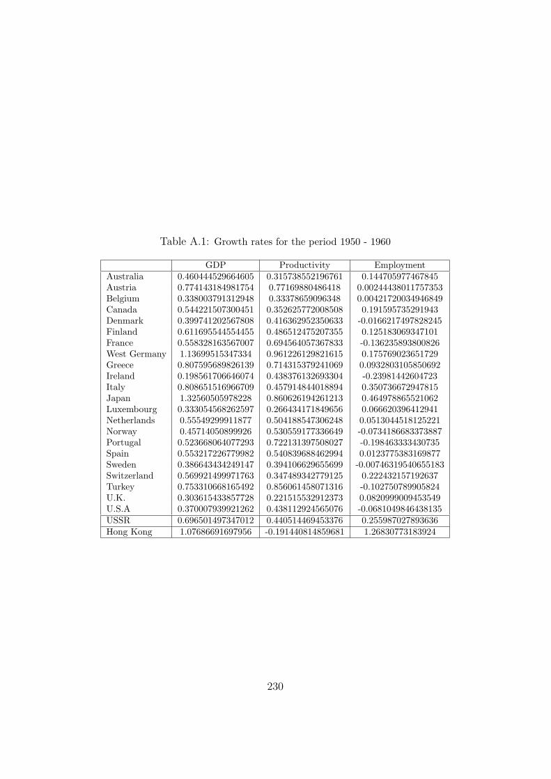
Table A.1: Growth rates for the period 1950 - 1960
GDP Productivity EmploymentAustralia 0.460444529664605 0.315738552196761 0.144705977467845Austria 0.774143184981754 0.77169880486418 0.00244438011757353Belgium 0.338003791312948 0.33378659096348 0.00421720034946849Canada 0.544221507300451 0.352625772008508 0.191595735291943Denmark 0.399741202567808 0.416362952350633 -0.0166217497828245Finland 0.611695544554455 0.486512475207355 0.125183069347101France 0.558328163567007 0.694564057367833 -0.136235893800826West Germany 1.13699515347334 0.961226129821615 0.175769023651729Greece 0.807595689826139 0.714315379241069 0.0932803105850692Ireland 0.198561706646074 0.438376132693304 -0.23981442604723Italy 0.808651516966709 0.457914844018894 0.350736672947815Japan 1.32560505978228 0.860626194261213 0.464978865521062Luxembourg 0.333054568262597 0.266434171849656 0.066620396412941Netherlands 0.55549299911877 0.504188547306248 0.0513044518125221Norway 0.45714050899926 0.530559177336649 -0.0734186683373887Portugal 0.523668064077293 0.722131397508027 -0.198463333430735Spain 0.553217226779982 0.540839688462994 0.0123775383169877Sweden 0.386643434249147 0.394106629655699 -0.00746319540655183Switzerland 0.569921499971763 0.347489342779125 0.222432157192637Turkey 0.753310668165492 0.856061458071316 -0.102750789905824U.K. 0.303615433857728 0.221515532912373 0.0820999009453549U.S.A 0.370007939921262 0.438112924565076 -0.0681049846438135USSR 0.696501497347012 0.440514469453376 0.255987027893636Hong Kong 1.07686691697956 -0.191440814859681 1.26830773183924
230
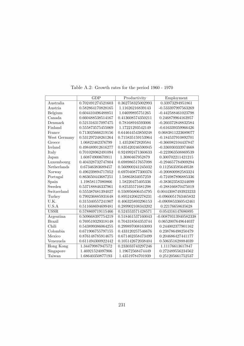
Table A.2: Growth rates for the period 1960 - 1970
GDP Productivity EmploymentAustralia 0.702491274521603 0.362758325002993 0.33973294951861Austria 0.582864170828165 1.11626216839143 -0.533397997563269Belgium 0.604410496488851 1.04699895751265 -0.442588461023798Canada 0.660488538514167 0.413608574350211 0.246879964163957Denmark 0.521316317097475 0.78168916593006 -0.260372848832584Finland 0.555873575455069 1.17221293542149 -0.616339359966426France 0.713025666219156 0.644644543850248 0.0683811223689077West Germany 0.531297248261264 0.715835159153964 -0.184537910892701Greece 1.06822462376799 1.43520672820584 -0.366982104437847Ireland 0.498489912616277 0.835420246590945 -0.336930333974668Italy 0.701028962491094 0.924992471360633 -0.223963508869539Japan 1.60874900670911 1.3080467952879 0.300702211421215Luxembourg 0.404328732747804 0.698986517657098 -0.294657784909294Netherlands 0.67346383689457 0.560900241245032 0.112563595649538Norway 0.496239894717052 0.697040877300376 -0.200800982583324Portugal 0.863650443687251 1.58863834057259 -0.724987896885336Spain 1.19858117080866 1.58220475405336 -0.383623583244699Sweden 0.537188846337961 0.82535571681298 -0.288166870475019Switzerland 0.555387681394027 0.550956806454795 0.00443087493923233Turkey 0.799236885931648 0.895242062278231 -0.0960051763465832U.K. 0.315340557241907 0.406325893296153 -0.0909853360542461U.S.A 0.511668694699481 0.289902108343202 0.22176658635628USSR 0.578869719115466 0.524553571428571 0.054316147686895Argentina 0.509668397754219 0.518461537160043 -0.00879313940582338Brazil 0.769519329318148 0.704318564353744 0.0652007649644037Chili 0.543899386064255 0.299897008163093 0.244002377901162Colombia 0.671906755797155 0.433120257546676 0.238786498250479Mexico 0.876148785914675 0.671462358473499 0.204686427441177Venezuela 0.611494300922442 0.105142672038404 0.506351628884039Hong Kong 1.34479987947572 0.233033743297246 1.11176613617847Singapore 1.46921524097906 1.19672568474449 0.272489556234562Taiwan 1.68640350877193 1.43519784701939 0.251205661752537
231
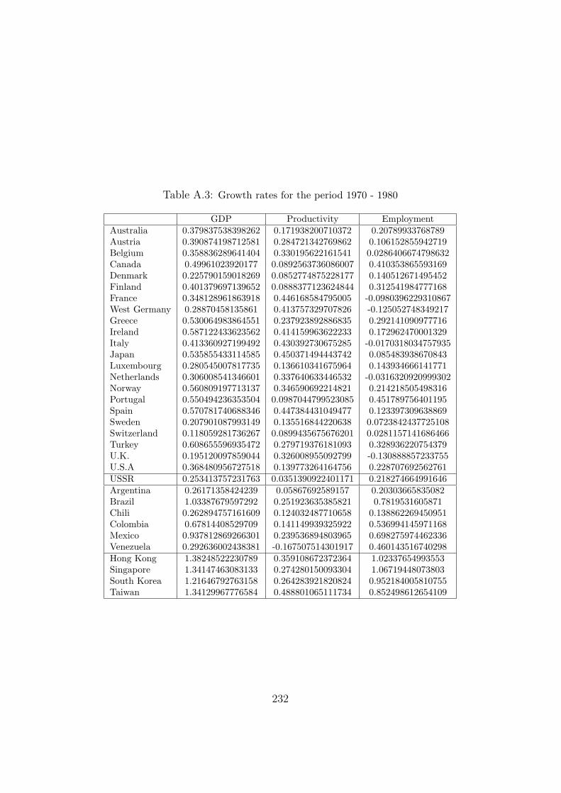
Table A.3: Growth rates for the period 1970 - 1980
GDP Productivity EmploymentAustralia 0.379837538398262 0.171938200710372 0.20789933768789Austria 0.390874198712581 0.284721342769862 0.106152855942719Belgium 0.358836289641404 0.330195622161541 0.0286406674798632Canada 0.49961023920177 0.0892563736086007 0.410353865593169Denmark 0.225790159018269 0.0852774875228177 0.140512671495452Finland 0.401379697139652 0.0888377123624844 0.312541984777168France 0.348128961863918 0.446168584795005 -0.0980396229310867West Germany 0.28870458135861 0.413757329707826 -0.125052748349217Greece 0.530064983864551 0.237923892886835 0.292141090977716Ireland 0.587122433623562 0.414159963622233 0.172962470001329Italy 0.413360927199492 0.430392730675285 -0.0170318034757935Japan 0.535855433114585 0.450371494443742 0.085483938670843Luxembourg 0.280545007817735 0.136610341675964 0.143934666141771Netherlands 0.306008541346601 0.337640633446532 -0.0316320920999302Norway 0.560809197713137 0.346590692214821 0.214218505498316Portugal 0.550494236353504 0.0987044799523085 0.451789756401195Spain 0.570781740688346 0.447384431049477 0.123397309638869Sweden 0.207901087993149 0.135516844220638 0.0723842437725108Switzerland 0.118059281736267 0.0899435675676201 0.0281157141686466Turkey 0.608655596935472 0.279719376181093 0.328936220754379U.K. 0.195120097859044 0.326008955092799 -0.130888857233755U.S.A 0.368480956727518 0.139773264164756 0.228707692562761USSR 0.253413757231763 0.0351390922401171 0.218274664991646Argentina 0.26171358424239 0.05867692589157 0.20303665835082Brazil 1.03387679597292 0.251923635385821 0.7819531605871Chili 0.262894757161609 0.124032487710658 0.138862269450951Colombia 0.67814408529709 0.141149939325922 0.536994145971168Mexico 0.937812869266301 0.239536894803965 0.698275974462336Venezuela 0.292636002438381 -0.167507514301917 0.460143516740298Hong Kong 1.38248522230789 0.359108672372364 1.02337654993553Singapore 1.34147463083133 0.274280150093304 1.06719448073803South Korea 1.21646792763158 0.264283921820824 0.952184005810755Taiwan 1.34129967776584 0.488801065111734 0.852498612654109
232
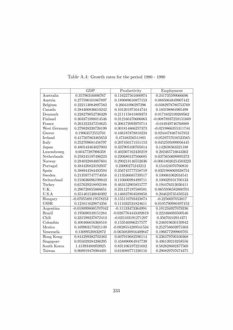
Table A.4: Growth rates for the period 1980 - 1990
GDP Productivity EmploymentAustralia 0.35796316006767 0.116227561000974 0.241735599066696Austria 0.277596101867897 0.189089616877153 0.0885064849907442Belgium 0.222113084897583 0.26041096297296 -0.0382978780753769Canada 0.284400836610242 0.101201971644744 0.183198864965498Denmark 0.228279052736329 0.211115841809373 0.0171632109269562Finland 0.303371098014546 0.312160470606063 -0.00878937259151669France 0.261222347210625 0.306172093970714 -0.044949746760089West Germany 0.279828230726199 0.301814866257373 -0.0219866355311744Greece 0.19063572552701 0.166187878810224 0.0244478467167852Ireland 0.417507863465653 0.47348356511801 -0.0559757016523565Italy 0.252709681456797 0.207450171551153 0.0452595099056445Japan 0.480543464027003 0.337905100705814 0.142638363321188Luxembourg 0.60477287906358 0.402307162420219 0.202465716643362Netherlands 0.258245197496223 0.220680127506685 0.0375650699895373Norway 0.284032884007604 0.290213146552636 -0.00618026254503223Portugal 0.384426823192937 0.23000275243212 0.154424070760816Spain 0.388944584492594 0.356745777558719 0.0321988069338754Sweden 0.213597747774058 0.113536685739517 0.100061062034541Switzerland 0.210636096199843 0.110606994499711 0.100029101700133Turkey 0.657629218892188 0.463152905855777 0.194476313036411U.K. 0.296720855866651 0.231127197580581 0.0655936582860701U.S.A 0.351461540040392 0.146837804589858 0.204623735450533Hungary -0.0705589119578253 0.155110793423874 -0.2256697053817USSR 0.121611629874356 0.111032531824611 0.0105790980497453Argentina -0.0100998065707042 -0.11133473364994 0.101234927079236Brazil 0.195690249151284 -0.0267764443492619 0.222466693500546Chili 0.331599237872413 -0.025103191271297 0.35670242914371Colombia 0.400466616368518 0.153546986217577 0.246919630150942Mexico 0.169903175021149 -0.0828554289541534 0.252758603975303Venezuela 0.13099520832872 -0.0656820916409847 0.196677299969705Hong Kong 0.844299382702482 0.607919682596114 0.236379700106368Singapore 0.955029284206295 0.458890064947739 0.496139219258556South Korea 1.41393488959925 0.831106197221682 0.582828692377569Taiwan 0.908919478904491 0.618089771230116 0.290829707674375
233
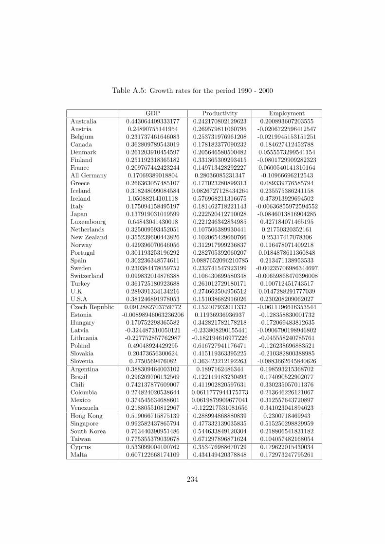
Table A.5: Growth rates for the period 1990 - 2000
GDP Productivity EmploymentAustralia 0.443064409333177 0.242170802129623 0.200893607203555Austria 0.24890755141954 0.269579811060795 -0.0206722596412547Belgium 0.231737461646083 0.253731976961208 -0.0219945153151251Canada 0.362809789543019 0.178182377090232 0.184627412452788Denmark 0.261203910454597 0.205646580500482 0.0555573299541154Finland 0.251192318365182 0.331365309293415 -0.0801729909282323France 0.209767442423244 0.149713428292227 0.0600540141310164All Germany 0.17069389018804 0.28036085231347 -0.10966696212543Greece 0.266363057485107 0.177023280899313 0.089339776585794Iceland 0.318248099084584 0.0826727128434264 0.235575386241158Ireland 1.05088214101118 0.576968211316675 0.473913929694502Italy 0.175094158495197 0.181462718221143 -0.00636855972594552Japan 0.137919031019599 0.222520412710028 -0.0846013816904285Luxembourg 0.64843041430018 0.221246342834985 0.427184071465195Netherlands 0.325009593452051 0.107506389930441 0.21750320352161New Zealand 0.355239600443826 0.102065429660766 0.25317417078306Norway 0.429396070646056 0.312917999236837 0.116478071409218Portugal 0.301193253196292 0.282705392060207 0.0184878611360848Spain 0.302236348574611 0.0887652096210785 0.213471138953533Sweden 0.230384478059752 0.232741547923199 -0.00235706986344697Switzerland 0.099832014876388 0.106430699580348 -0.00659868470396008Turkey 0.361725180923688 0.261012729180171 0.100712451743517U.K. 0.289391334134216 0.274662504956512 0.0147288291777039U.S.A 0.381246891978053 0.151038682916026 0.230208209062027Czech Republic 0.0912882703759772 0.152407932011332 -0.0611196616353544Estonia -0.00898946063236206 0.11936936936937 -0.128358830001732Hungary 0.170752298365582 0.342821782178218 -0.172069483812635Latvia -0.324487310050121 -0.233808290155441 -0.0906790198946802Lithuania -0.227752857762987 -0.182194616977226 -0.045558240785761Poland 0.49048924429295 0.616727941176471 -0.126238696883521Slovakia 0.20473656300624 0.415119363395225 -0.210382800388985Slovenia 0.2750569476082 0.363423212192263 -0.0883662645840626Argentina 0.388309464003102 0.1897162486344 0.198593215368702Brazil 0.296209706132569 0.122119183230493 0.174090522902077Chili 0.742137877609007 0.411902820597631 0.330235057011376Colombia 0.274824020538644 0.0611777944175773 0.213646226121067Mexico 0.374545634688601 0.0619879909677041 0.312557643720897Venezuela 0.218805510812967 -0.122217531081656 0.341023041894623Hong Kong 0.519066715875139 0.288994868880839 0.2300718469943Singapore 0.992582437865794 0.477332139035835 0.515250298829959South Korea 0.763440390951486 0.544633849120304 0.218806541831182Taiwan 0.775355379039678 0.671297896871624 0.104057482168054Cyprus 0.533099004100762 0.353476988670729 0.179622015430034Malta 0.607122668174109 0.434149420378848 0.172973247795261
234
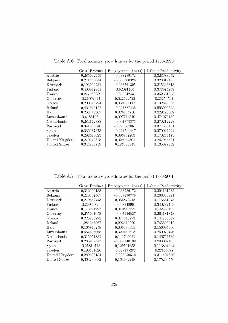
Table A.6: Total industry growth rates for the period 1980-1990
Gross Product Employment (hours) Labour ProductivityAustria 0,285092455 -0,033289172 0,323683052Belgium 0,241208644 -0,065700326 0,328019485Denmark 0,193033281 -0,033561305 0,215333818Finland 0,406017951 0,02071406 0,377974257France 0,277983239 -0,059242431 0,352661653Germany 0,26062392 0,022622522 0,23259592Greece 0,200315294 0,059705117 0,132848055Ireland 0,464915122 -0,057827425 0,553990255Italy 0,263719907 0,026884756 0,229475562Luxembourg 0,61851051 0,097714519 0,474278482Netherlands 0,284672388 -0,001778873 0,270212223Portugal 0,341059648 -0,022587867 0,371565131Spain 0,336187373 -0,024711447 0,370022924Sweden 0,292670623 0,093947283 0,170255473United Kingdom 0,279740325 0,029154301 0,247955521United States 0,344829759 0,183796545 0,135987552
Table A.7: Total industry growth rates for the period 1990-2001
Gross Product Employment (hours) Labour ProductivityAustria 0,312109183 -0,033289172 0,394131985Belgium 0,216137467 -0,037290779 0,263336921Denmark 0,219652743 0,035870418 0,173661975Finland 0,20936891 -0,098349961 0,340782493France 0,173221993 0,010840922 0,15872565Germany 0,255041653 -0,007156527 0,264181873Greece 0,226889723 0,074615773 0,141756067Ireland 1,284345367 0,293610229 0,765503012Italy 0,165918258 0,003893831 0,156695666Luxembourg 0,654595065 0,322459623 0,250970446Netherlands 0,315051831 0,141746021 0,146752739Portugal 0,285932447 -0,005140199 0,293002103Spain 0,25810718 0,129501653 0,113804094Sweden 0,199321626 -0,027395282 0,22664072United Kingdom 0,289638134 -0,022550542 0,311427356United States 0,368283682 0,164082248 0,175290556
235

236
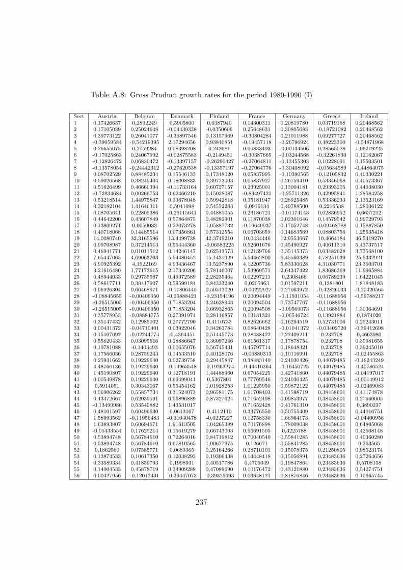
Table A.8: Gross Product growth rates for the period 1980-1990 (I)
Sect Austria Belgium Denmark Finland France Germany Greece Ireland1 0,17426637 0,2892249 0,5905800 0,0387940 0,14300311 0,20819780 0,03719168 0,204685622 0,17105039 0,25024648 -0,04439338 -0,0350606 0,25648631 0,30805683 -0,18721082 0,204685623 0,39773122 0,26041077 -0,36897546 0,13157969 -0,30804284 0,21011988 0,09277727 0,204685624 -0,39059584 -0,54219395 2,17294656 0,93840851 -0,19457118 -0,26796924 0,48223300 -0,548719685 0,26655075 0,2159284 0,08398208 0,242681 0,00883493 -0,00134506 0,28565528 1,062192256 -0,17025863 0,24067992 -0,02875583 -0,2149451 -0,30387665 -0,03244568 -0,32261830 0,121620677 -0,12826472 0,06830472 -0,13397157 -0,26290427 -0,27064811 -0,13455303 0,10228091 0,155035018 -0,13578054 -0,24442312 -0,27620538 -0,13357197 -0,27064776 -0,30408092 -0,05634589 -0,448640759 0,08702529 0,88485234 0,15546133 0,17348020 0,05837995 -0,10390565 -0,12105832 0,4033022110 0,59026568 0,38249404 0,18008833 0,39773003 0,05837927 0,26759410 0,53346068 0,4057336711 0,51626499 0,46660394 -0,11733164 0,60727157 0,23925001 0,13004181 0,29393205 0,4493803012 -0,72834684 0,00266753 0,62466210 0,15028087 -0,83497421 -0,25711326 0,42995841 1,2858425813 0,53218514 1,44975847 0,33678048 0,59942818 0,35181947 0,28925485 0,53336233 2,1352316914 0,32182104 1,41646311 0,5041098 0,54552283 0,0916134 0,49788500 0,2216538 1,2803612215 0,08705641 0,22805386 -0,26115641 0,44881055 0,23186721 -0,01174143 0,02836952 0,663721216 0,44642200 0,43607849 0,57864875 0,48282901 0,11870038 0,02301646 0,14579542 0,9972979317 0,13809271 0,0050033 0,22073278 1,05887732 -0,16640937 0,17052748 -0,09468788 0,1588785018 0,40718068 0,14485514 0,07356861 0,57312554 0,06703659 0,14683569 0,08803756 1,2563541819 14,0080740 32,3165596 13,4499738 42,3749210 10,0434446 12,9553667 10,4664184 46,541927020 0,99708987 0,37214513 0,55444360 -0,06583225 0,52601676 0,45490927 0,40611310 5,4373751721 0,46941771 0,01011512 0,14246147 0,62513573 0,12139766 0,35145375 0,03482628 3,7356810022 7,65447065 4,69063203 5,54480452 15,1431929 5,54462800 6,45560389 4,78251039 25,533292123 6,90925392 4,1922169 4,93436467 13,5237890 4,12205736 5,83330628 4,31030771 23,360370124 3,21616480 1,77173615 2,17340206 5,78146007 1,53969571 2,64347422 1,83686369 11,996588425 0,48944033 0,29735567 0,49372589 2,28235464 0,02297211 0,2308466 0,06789239 1,6422104526 0,58617711 0,38417907 0,59599184 0,84333240 0,0205963 0,01597211 0,1381801 1,8184818327 0,06926304 0,66468971 -0,17806445 0,50512020 -0,00222927 0,27063972 -0,42826033 -0,2042056528 -0,08845655 -0,00406950 -0,26888421 -0,23154196 0,20094449 -0,11931054 -0,11688956 -0,5978821729 -0,26515005 -0,00406950 0,71853204 3,24628943 0,20094504 0,73747767 -0,1168895630 -0,26515005 -0,00406950 0,71853204 0,66932865 0,20094508 -0,09569073 -0,11688956 1,3036469131 0,35778953 -0,08884775 0,27391974 0,28116857 0,13131321 -0,06546724 0,13921884 0,187402032 0,35147432 0,12985002 0,27772790 0,4110733 0,82626662 0,16294519 0,52731006 0,2524301133 0,00431372 -0,04710401 0,03922046 0,34263784 0,08640428 -0,01041372 -0,03402720 -0,3941269834 0,15107092 -0,02244774 -0,4364451 0,51445773 0,28488422 0,22409211 0,232708 0,466398035 0,55820433 0,03095616 0,28886647 0,36097246 0,61561317 0,17878754 0,232708 0,3998165536 0,19781088 -0,1403493 0,00655076 0,56745431 0,45797714 0,18648321 0,232708 0,3924501037 0,17566036 0,28759243 0,14533510 0,40128076 -0,06880313 0,10116991 0,232708 -0,0245586338 0,25931662 0,19229640 0,02739758 0,29445847 0,38483140 0,24030426 0,44079485 -0,1624324939 4,48766136 0,19229640 -0,14963548 -0,19263274 -0,44410364 -0,16450725 0,44079485 -0,4078652440 1,45190807 0,19229640 0,12718191 1,44488960 0,67054225 0,42741860 0,44079485 -0,0419701741 0,00549878 0,19229640 0,69499041 0,5367801 0,77769546 0,24030425 0,44079485 -0,0014991242 0,5914051 0,30343067 0,55454162 1,01928253 1,01225950 0,59872122 0,44079485 -0,0246908343 0,56906262 0,55857734 0,31524073 0,96581175 1,01708403 0,41598719 0,38458601 0,4117487844 0,43472667 0,62035591 0,56896889 0,87327624 0,71652498 0,09853977 0,38458601 0,2766000545 -0,13499986 0,53540882 1,43531017 0,71652428 0,41761310 0,38458601 0,389023746 0,48101597 0,60496630 0,0613167 0,4112110 0,33776550 0,50755409 0,38458601 0,4401675147 1,58993562 -0,11956483 -0,31040478 -0,0227227 0,12758330 1,66964173 0,38458601 -0,0440095848 1,63893807 0,60694671 1,91613505 1,04265389 0,70176898 1,78009038 0,38458601 0,6480506849 -0,05433554 0,17625214 0,15619279 0,66743003 0,96691505 0,3225788 0,38458601 0,4260814850 0,53894748 0,56784610 0,72264016 0,84719812 0,70040540 0,55841285 0,38458601 0,4036028051 0,53894748 0,56784610 0,67810565 1,00677975 0,126671 0,55841285 0,38458601 0,26356552 0,1862560 0,07585771 0,0683365 0,25164266 0,28710101 0,15078375 0,21250805 0,9852317453 0,13874533 0,10617350 0,12038293 0,19306438 0,14448418 0,15056891 0,23483636 0,2726465654 0,33589334 0,41859793 0,1998931 0,40517786 0,4705049 0,19847864 0,23483636 0,570815855 0,14004533 0,45878719 0,34909289 0,47089690 0,10176472 0,43121880 0,23483636 0,5427475156 0,00427956 -0,12012431 -0,39447073 -0,39325693 0,03648121 0,81870846 0,23483636 0,10665745
237

238
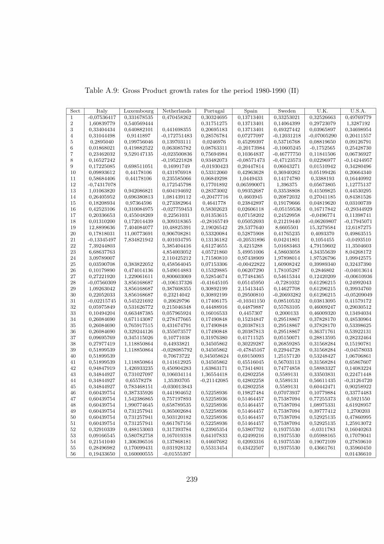
Table A.9: Gross Product growth rates for the period 1980-1990 (II)
Sect Italy Luxembourg Netherlands Portugal Spain Sweden U.K. U.S.A.1 -0,07536417 0,331678535 0,470458262 0,30324695 0,13713401 0,33253021 0,32526663 0,497697792 1,60839779 0,540569444 0,31751275 0,13713401 0,14064399 0,29723079 1,32871923 0,33404434 0,640882101 0,441698355 0,20695183 0,13713401 0,49327442 0,03965897 0,346989544 0,31044498 0,9141897 -0,172751483 0,28576784 0,07277097 -0,12031218 -0,07005290 0,204115575 0,2895040 0,199756046 0,139703111 0,0246976 0,45299397 0,53716768 0,08819650 0,091267916 0,01868021 0,419882522 0,063085782 0,08763311 -0,20173984 -0,10605245 -0,1752565 0,254287307 0,23462032 9,529147135 -0,023500836 0,75694984 0,10364837 -0,46777750 0,11841506 0,067369278 0,16527242 -0,195221828 0,93482073 -0,08571473 -0,47123573 0,02296977 -0,142449579 0,17225085 0,698511051 0,16991749 -0,01930423 0,20447814 0,06043271 0,01510942 0,3428049610 0,09893612 0,44178106 0,431976918 0,53312060 0,42963628 0,36940262 0,05199426 0,2066434011 0,58684406 0,44178106 0,235585066 0,06849298 1,0449433 0,14174780 0,3388193 0,1644099212 -0,74317078 0,172545798 0,17701892 0,065990071 1,396375 0,05673805 1,1277513713 1,01063820 0,942086821 0,604194692 0,28373002 0,99352687 0,33538808 0,41509825 0,4453029514 0,26405952 0,696380813 1,081439112 -0,20477716 0,4603945 0,20872032 0,27041185 0,8438152615 0,18208934 0,97364596 0,273382964 0,4641778 0,23842897 0,19179666 0,04819620 0,0310073916 0,42523106 0,310084975 -0,027759453 0,58302623 0,02606118 -0,05159536 0,16717842 -0,2934492917 0,20336653 0,455048269 0,22561031 0,01353615 0,07158202 0,24529958 -0,0496774 0,1139874118 0,01310200 0,172014439 0,309318365 -0,28165749 0,05052693 0,21219440 -0,06269807 -0,1794507119 12,8899636 7,404084077 10,48825391 2,19026542 29,5377640 8,6605501 15,3279584 12,618727520 0,17818031 11,00773691 0,906708281 0,53320084 0,52875908 0,41765235 0,4093370 0,4986351521 -0,13345497 7,834821942 0,401034795 0,13136182 -0,20531896 0,04241801 0,1054455 -0,049351022 7,39244803 5,385404416 4,61274655 3,4215288 5,01683463 4,79159602 11,350460323 6,68637763 4,854003052 4,05721860 5,49951006 4,58603058 4,34355639 8,0426817224 3,09789007 2,110425212 1,71580810 0,97438909 1,97898014 1,97526796 1,0994257525 0,03590708 0,383822052 0,458564045 0,07153306 -0,00422822 1,60908242 0,39989340 0,3243739026 0,10179890 0,474014136 0,549014883 0,15329885 0,06207290 1,78105287 0,2846802 -0,0401361427 0,27221920 1,229061611 0,800603069 0,52854674 0,77484365 0,54615344 0,12420209 -0,0061093628 -0,07560309 3,856168687 -0,106137326 -0,41645105 0,05145950 -0,7281032 0,61296215 0,2499204329 1,09263042 3,856168687 0,387608355 0,30892199 2,15413445 0,14627708 0,61296215 0,3993476030 0,22052033 3,856168687 0,23214042 0,30892199 0,29500810 -0,20693282 0,61296215 -0,0520904931 -0,02215745 0,545221692 0,20629796 0,17406175 -0,10341150 0,08510532 0,03813095 0,4157917232 0,05975849 0,531626772 0,215046348 0,44488916 0,44879887 0,55763105 0,46009247 0,2903051233 0,10494204 0,663487385 0,057965924 0,16016533 0,4457307 0,2000133 0,46009320 0,1349403434 0,26084690 0,671143087 0,278477665 0,17490848 0,15234847 0,29518867 0,37828170 0,4853096435 0,26084690 0,765917515 0,431674791 0,17490848 0,20387813 0,29518867 0,37828170 0,5339862536 0,26084690 0,329244126 0,355073577 0,17490848 0,20387813 0,29518867 0,36371761 0,5392213137 0,09695769 0,345115026 0,10771038 0,31976380 0,41711525 0,05150071 0,28813595 0,2823246438 0,27977419 1,118850864 0,44933821 0,34505862 0,30229287 0,26859285 0,31568284 0,1519078139 0,51899539 1,118850864 -0,028085792 0,34505862 -0,47845167 0,22944728 0,31568284 -0,0457803340 0,51899539 0,70673722 0,345058624 0,69150093 1,25157120 0,53248427 1,0670686141 0,51899539 1,118850864 0,141612925 0,34505862 0,45516045 0,56703113 0,31568284 0,6586760742 0,94847919 1,426933235 0,450904283 1,63863171 0,73414801 0,74774858 0,58883327 0,1408322443 0,34844927 0,731027097 0,106034114 1,36554418 0,42802258 0,5589131 0,33503831 0,2247144844 0,34844927 0,65578278 1,35393705 -0,21142085 0,42802258 0,5589131 0,56611435 -0,3126472045 0,34844927 0,783468151 -0,030013843 0,42802258 0,5589131 0,60442471 0,9025892246 0,60439754 0,387335926 0,441904652 0,52258936 0,19827484 0,07073937 0,10779884 0,3377448347 0,60439754 1,542386865 0,757197893 0,52258936 0,51464457 0,75387094 0,77255373 0,592155048 0,60439754 1,990774645 0,658789535 0,52258936 0,51464457 0,75387094 1,08975331 4,6192895749 0,60439754 0,731257941 0,365002684 0,52258936 0,51464457 0,75387094 0,39777412 1,270020350 0,60439754 0,731257941 0,503120182 0,52258936 0,51464457 0,75387094 0,52925135 0,4786099551 0,60439754 0,731257941 0,661767156 0,52258936 0,51464457 0,75387094 0,52925135 1,2591307252 0,32910339 0,488153003 0,317393784 0,23905354 0,53807702 0,19375530 -0,0311783 0,1604026353 0,09166545 0,580782758 0,167019318 0,64107833 0,42499216 0,19375530 0,05988165 0,1707904154 0,21541040 1,306396516 0,137868181 0,44607682 0,42093316 0,19375530 0,19072109 0,2785961055 0,28496982 0,170099431 0,031928132 0,55313454 0,43422507 0,19375530 0,43661761 0,3596045056 0,19433650 0,160000555 -0,01555397 0,01436610
239

240
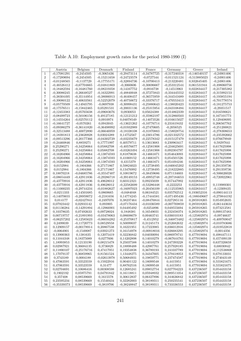
Table A.10: Employment growth rates for the period 1980-1990 (I)
Austria Belgium Denmark Finland France Germany Greece Ireland1 -0,17081291 -0,2454505 -0,3065436 -0,29473114 -0,34787725 -0,317240318 -0,146540157 -0,249014062 -0,17289694 -0,2454505 -0,15211658 -0,24723578 -0,0727544 -0,011521124 -0,513885023 -0,249014063 -0,01248565 -0,1137729 -0,17755171 -0,32894736 -0,10700413 -0,213220481 0,932645405 -0,249014064 -0,46526412 -0,67704665 -0,04841869 -0,3060606 -0,30696667 -0,253312544 0,061531944 -0,4980607565 -0,18482594 -0,16481760 -0,08219358 -0,14167752 -0,0916738 -0,14513963 0,022834417 -0,2173053826 -0,30086245 -0,26648527 -0,16322991 -0,48840048 -0,37275843 -0,334445552 0,022834417 -0,3159921537 -0,38304495 -0,35144954 -0,38006913 -0,46408457 -0,36575959 -0,344541689 0,022834417 -0,1938551948 -0,39080122 -0,40633561 -0,52252079 -0,40750672 -0,33376717 -0,470553413 0,022834417 -0,7017785749 -0,05770509 -0,14945795 -0,0697938 -0,30998431 -0,25880643 -0,138020423 0,022834417 -0,18127575310 -0,17576511 -0,15842465 0,05291531 -0,20031136 -0,25315954 -0,043108494 0,022834417 -0,2935151711 -0,12453383 -0,05765638 -0,09683676 0,0930053 0,05624388 -0,014862339 0,022834417 0,01659062112 -0,08499723 -0,50106156 0,49127185 -0,12121212 -0,35962197 -0,312860503 0,022834417 0,16710177313 -0,14554264 -0,02570112 0,0910974 0,04078549 -0,14073526 -0,016615027 0,022834417 0,12940809514 -0,16641727 -0,0570261 0,0943045 -0,13621262 -0,10776714 0,231619432 0,022834417 0,20656776215 -0,09386279 -0,36141820 -0,36498992 -0,01932989 -0,27470605 -0,2056525 0,022834417 -0,25120082116 -0,32513488 -0,40072890 -0,06646959 -0,18108108 -0,31870883 -0,158028754 0,022834417 -0,27830865317 -0,18391813 -0,23620928 0,03024289 0,14752567 -0,23014786 -0,021332572 0,022834417 -0,23539266218 -0,09513296 -0,20177366 -0,04302729 -0,03235679 -0,22578342 -0,015127479 0,022834417 0,07667994919 -0,24460846 0,8859271 0,17771997 0,40579711 0,13613683 0,230963417 0,022834417 0,5929764120 0,25290271 -0,34258064 0,05882708 -0,40576677 -0,12581908 -0,234625691 0,022834417 0,61762599821 0,25290271 -0,34258064 0,05882708 -0,03263494 -0,12581908 0,092304797 0,022834417 0,61762599822 -0,16204966 -0,34258064 -0,13874593 0,81879638 -0,14661671 0,054643093 0,022834417 0,61762599823 -0,16204966 -0,34258064 -0,13874593 0,41069152 -0,14661671 0,054501526 0,022834417 0,61762599824 -0,16204966 -0,34258064 -0,13874593 0,4315379 -0,14661671 0,054494246 0,022834417 0,61762599825 0,0152984 -0,1804366 0,27171867 0,59824023 -0,12738495 -0,040045202 0,022834417 0,29135973626 0,0152984 -0,1804366 0,27171867 0,13476992 -0,12738495 -0,218222885 0,022834417 0,29135973627 0,18870218 -0,04685786 -0,35547407 0,10819672 -0,38459686 0,071134603 0,022834417 -0,50662602628 -0,08654449 -0,42911836 -0,29286718 -0,39149153 -0,49952748 -0,297184653 0,022834417 -0,72092296129 -0,43770916 -0,42911836 0,49628012 0,60312321 0,09235039 0,357447992 0,02283441730 -0,43770916 -0,42911836 0,49628012 -0,22582699 -0,53286448 -0,2222253 0,022834417 0,11998930131 -0,11000235 -0,29744234 -0,01882627 -0,16097023 -0,20456109 -0,112535965 0,022834417 -0,1230943532 -0,0211333 -0,14501685 0,0869665 -0,0484048 0,06184521 0,035792512 0,193652316 -0,09014411333 -0,14070655 -0,28959072 -0,2181656 0,14774245 -0,17444581 -0,071495436 -0,188049667 -0,27984419234 0,014177 -0,02427841 -0,2497076 0,38237464 -0,08476844 0,027285116 0,285918265 0,05495263535 0,07923442 0,02933142 0,093905 -0,07176434 -0,01036589 -0,007769859 0,285918265 -0,06144363436 0,01136284 -0,14291894 -0,12966901 0,04495492 -0,0254896 0,049555694 0,285918265 0,07321258137 0,10378635 0,07492633 0,09728024 0,1848381 0,16549031 0,232458374 0,285918265 0,09913748338 0,00719757 -0,21891993 -0,03478063 0,08608679 0,00463741 0,036010183 -0,125802974 -0,0974663739 -0,06257202 -0,12585623 -0,06034282 -0,25370817 -0,4512952 -0,346873482 -0,125802974 -0,40976904740 0,2499039 -0,11720773 0,08529558 0,50099037 0,31245173 0,252682632 -0,125802974 -0,01078368641 0,12909157 -0,00178914 0,20867538 0,16221951 0,17223985 0,036012916 -0,125802974 -0,01952281842 -0,0064901 -0,1549087 0,03921273 0,16154978 -0,00918016 0,026683295 -0,125802974 -0,001435643 0,13900363 0,1381635 0,12075419 0,32236842 0,04030094 0,086978741 0,477919694 0,49844711144 0,11044348 0,18375089 0,0277606 0,14202898 0,14010279 -0,067644761 0,477919694 0,45749913945 1,18993853 0,12133190 0,08215478 9,25037588 0,14010279 0,247393228 0,477919694 0,63732065946 0,02987921 0,36684135 0,3736829 0,18898488 0,42987761 0,257928185 0,477919694 0,6803084247 0,11890107 -0,25176716 0,47417951 0,19354838 0,36789193 0,241037789 0,477919694 -0,11253880848 1,17079137 0,36859965 0,81561524 1,13448275 0,34347605 0,579418053 0,477919694 0,67913303149 0,3743189 0,0004188 -0,02613978 0,50684931 0,19859771 0,237474587 0,477919694 0,27404314950 0,47063591 0,33523559 0,15922916 0,90401122 0,18099548 0,4415951 0,477919694 0,55582167551 0,47063591 0,33523559 0,31477 0,88762516 0,18099548 0,4415951 0,477919694 0,55582167552 0,02704691 0,10686416 0,00308598 0,12685241 0,09852754 0,027704223 0,437236507 0,05443315853 0,1902192 0,05975791 0,04791842 0,16118811 0,05948932 0,089511054 0,437236507 0,05443315854 0,357408 0,08539669 0,1615578 0,30612837 0,06427896 0,344636842 0,437236507 0,05443315855 0,23595234 0,08539669 0,15540434 0,32282003 0,38189311 0,250235541 0,437236507 0,05443315856 -0,35339373 0,08539669 -0,3819706 -0,38248847 0,38189311 0,733336553 0,437236507 0,054433158
241

242
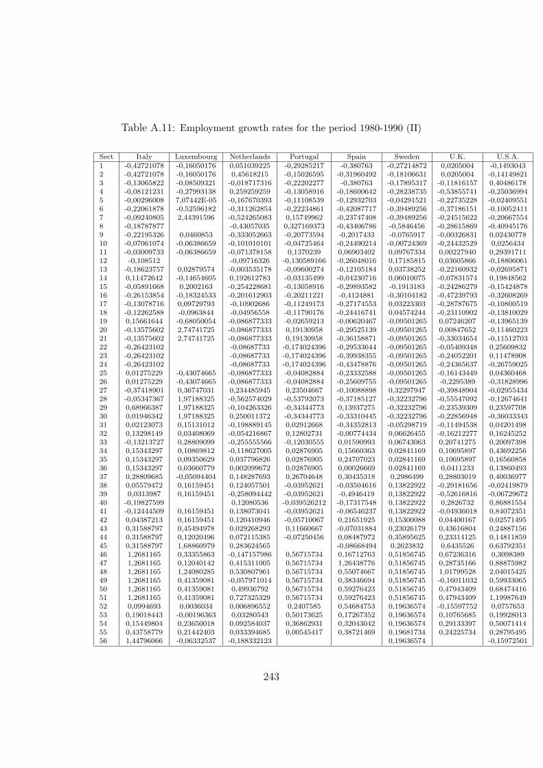
Table A.11: Employment growth rates for the period 1980-1990 (II)
Sect Italy Luxembourg Netherlands Portugal Spain Sweden U.K. U.S.A.1 -0,42721078 -0,16050176 0,051039225 -0,29285217 -0,380763 -0,27214872 0,0205004 -0,14930432 -0,42721078 -0,16050176 0,45618215 -0,15026595 -0,31960492 -0,18106631 0,0205004 -0,141498213 -0,13065822 -0,08509321 -0,018717316 -0,22202277 -0,380763 -0,17895317 -0,11816157 0,404861784 -0,08121231 -0,27993138 0,259259259 -0,13058916 -0,18600642 -0,28238735 -0,53855741 -0,250369945 -0,00296008 7,07442E-05 -0,167670393 -0,11108539 -0,12932703 -0,04291521 -0,22735228 -0,024095516 -0,22061878 -0,52596182 -0,311262854 -0,22234861 -0,42087717 -0,39489256 -0,37186151 -0,100524117 -0,09240805 2,44391596 -0,524265083 0,15749962 -0,23747408 -0,39489256 -0,24515622 -0,206675548 -0,18787877 -0,43057035 0,327169373 -0,43406786 -0,5846456 -0,28615869 -0,409451769 -0,22195326 0,0460853 -0,333052663 -0,20773594 -0,2017433 -0,0765917 -0,00326831 0,0243077810 -0,07061074 -0,06386659 -0,101010101 -0,04725464 -0,24490214 -0,00724369 -0,24432529 0,025643411 -0,03009733 -0,06386659 -0,071378158 0,1370239 0,06903402 0,09767334 0,00227940 0,2939171112 -0,108512 -0,09716326 -0,130589166 -0,26048016 0,17185815 0,03605866 -0,1880606113 -0,18623757 0,02879574 -0,003535178 -0,09600274 -0,12105184 0,03738252 -0,22160932 -0,0269587114 0,11472642 -0,14654605 0,192612783 -0,03135499 -0,04230716 0,06010075 -0,07831574 0,1984856215 -0,05891668 0,2002163 -0,254228681 -0,13058916 -0,29893582 -0,1913183 -0,24286279 -0,1542487816 -0,26153854 -0,18324533 -0,201612903 -0,20211221 -0,4124881 -0,30104182 -0,47239793 -0,3260826917 -0,13078716 0,09729793 -0,10902686 -0,11249173 -0,27174553 0,03223303 -0,28787675 -0,1080051918 -0,12262588 -0,0963844 -0,04956558 -0,11790176 -0,24416741 0,04574244 -0,23110902 -0,1381002919 0,15661644 -0,68050054 -0,086877333 -0,02659213 -0,00620467 -0,09501265 0,07246207 -0,1396513920 -0,13575602 2,74741725 -0,086877333 0,19130958 -0,29525139 -0,09501265 0,00847652 -0,1146022321 -0,13575602 2,74741725 -0,086877333 0,19130958 -0,36158871 -0,09501265 -0,33034654 -0,1151270322 -0,26423102 -0,08687733 -0,174024396 -0,29533644 -0,09501265 -0,05409348 0,2560983223 -0,26423102 -0,08687733 -0,174024396 -0,39938355 -0,09501265 -0,24052201 0,1147890824 -0,26423102 -0,08687733 -0,174024396 -0,43478876 -0,09501265 -0,24365637 -0,2675902525 0,01275229 -0,43074665 -0,086877333 -0,04082884 -0,23332588 -0,09501265 -0,16143449 0,0436046826 0,01275229 -0,43074665 -0,086877333 -0,04082884 -0,25609755 -0,09501265 -0,2295389 -0,3182899627 -0,37418901 0,36747031 0,234485945 0,23504667 -0,10088898 0,32297947 -0,39848904 -0,0295543428 -0,05347367 1,97188325 -0,562574029 -0,53792073 -0,37185127 -0,32232796 -0,55547092 -0,1267464129 0,68966387 1,97188325 -0,104263326 -0,34344773 0,13937275 -0,32232796 -0,23539309 0,2359770830 0,01946342 1,97188325 0,250011372 -0,34344773 -0,33310445 -0,32232796 -0,22856948 -0,3603334331 0,02123073 0,15131012 -0,198889145 0,02912668 -0,34352813 -0,05298719 -0,11494538 0,0420149832 0,13298149 0,03408069 -0,054216867 0,12802731 -0,00774434 0,06626455 -0,16212277 0,1624525233 -0,13213727 0,28809099 -0,255555566 -0,12030555 0,01590993 0,06743063 0,20741275 0,2009739834 0,15343297 0,10869812 -0,118627005 0,02876905 0,15660363 0,02841169 0,10695897 0,4369225635 0,15343297 0,09350629 0,037796826 0,02876905 0,24707023 0,02841169 0,10695897 0,1656085836 0,15343297 0,03660779 0,002099672 0,02876905 0,00026669 0,02841169 0,0411233 0,1386049337 0,28809685 -0,05094404 0,148287693 0,26704648 0,30435318 0,2986499 0,28803019 0,4003697738 0,05579472 0,16159451 0,124057501 -0,03952621 -0,03504616 0,13822922 -0,29181656 -0,0241987939 0,0313987 0,16159451 -0,258094442 -0,03952621 -0,4946419 0,13822922 -0,52616816 -0,0672967240 -0,19827599 0,12080536 -0,039526212 -0,17317548 0,13822922 0,2826732 0,8688155441 -0,12444509 0,16159451 0,138073041 -0,03952621 -0,06546237 0,13822922 -0,04936018 0,8407235142 0,04387213 0,16159451 0,120410946 -0,05710067 0,21651925 0,15300088 0,04400167 0,0257149543 0,31588797 0,45494978 0,029268293 0,11660667 -0,07031884 0,23026179 0,43616804 0,2488715644 0,31588797 0,12020496 0,072115385 -0,07250456 0,08487972 0,35895625 0,23314125 0,1481185945 0,31588797 1,68860979 0,283624565 -0,08668494 0,2623832 0,6435526 0,6379235146 1,2681165 0,33355863 -0,147157986 0,56715734 0,16712763 0,51856745 0,67236316 0,309838947 1,2681165 0,12040142 0,415311005 0,56715734 1,26438776 0,51856745 0,28735166 0,8887598248 1,2681165 1,24080285 0,530807961 0,56715734 0,55074667 0,51856745 1,01799528 2,0401542549 1,2681165 0,41359081 -0,057971014 0,56715734 0,38346694 0,51856745 -0,16011032 0,5993306550 1,2681165 0,41359081 0,49936792 0,56715734 0,59276423 0,51856745 0,47943409 0,6847441651 1,2681165 0,41359081 0,727325329 0,56715734 0,59276423 0,51856745 0,47943409 1,1998764952 0,0994693 0,0036034 0,006896552 0,2407585 0,54684753 0,19636574 -0,15597752 0,075765353 0,19018443 -0,00196363 0,03280543 0,50173625 0,17267352 0,19636574 0,10765685 0,1992801354 0,15449804 0,23650018 0,092584037 0,36862931 0,32043042 0,19636574 0,29133397 0,5007141455 0,43758779 0,21442403 0,033394685 0,00545417 0,38721469 0,19681734 0,24225734 0,2879549556 1,44796066 -0,06332537 -0,188332123 0,19636574 -0,15972501
243

244
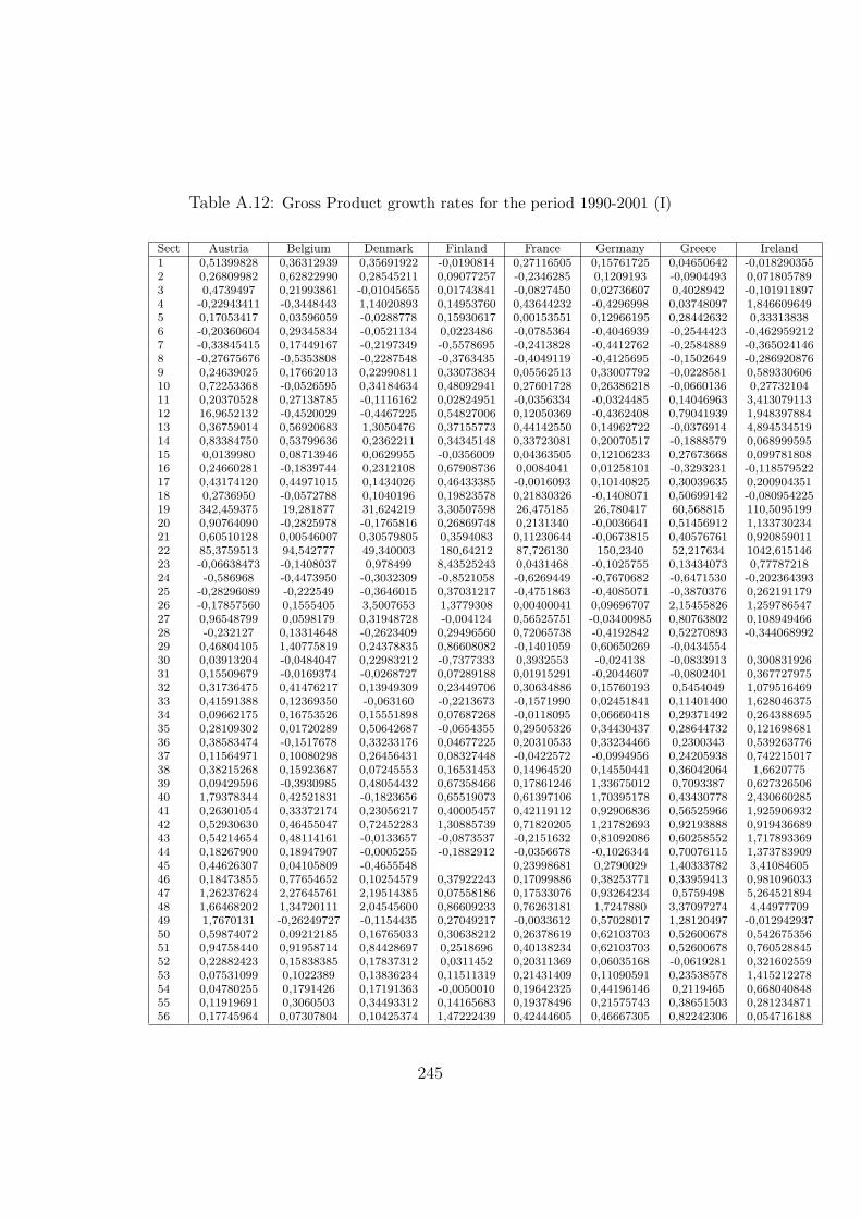
Table A.12: Gross Product growth rates for the period 1990-2001 (I)
Sect Austria Belgium Denmark Finland France Germany Greece Ireland1 0,51399828 0,36312939 0,35691922 -0,0190814 0,27116505 0,15761725 0,04650642 -0,0182903552 0,26809982 0,62822990 0,28545211 0,09077257 -0,2346285 0,1209193 -0,0904493 0,0718057893 0,4739497 0,21993861 -0,01045655 0,01743841 -0,0827450 0,02736607 0,4028942 -0,1019118974 -0,22943411 -0,3448443 1,14020893 0,14953760 0,43644232 -0,4296998 0,03748097 1,8466096495 0,17053417 0,03596059 -0,0288778 0,15930617 0,00153551 0,12966195 0,28442632 0,333138386 -0,20360604 0,29345834 -0,0521134 0,0223486 -0,0785364 -0,4046939 -0,2544423 -0,4629592127 -0,33845415 0,17449167 -0,2197349 -0,5578695 -0,2413828 -0,4412762 -0,2584889 -0,3650241468 -0,27675676 -0,5353808 -0,2287548 -0,3763435 -0,4049119 -0,4125695 -0,1502649 -0,2869208769 0,24639025 0,17662013 0,22990811 0,33073834 0,05562513 0,33007792 -0,0228581 0,58933060610 0,72253368 -0,0526595 0,34184634 0,48092941 0,27601728 0,26386218 -0,0660136 0,2773210411 0,20370528 0,27138785 -0,1116162 0,02824951 -0,0356334 -0,0324485 0,14046963 3,41307911312 16,9652132 -0,4520029 -0,4467225 0,54827006 0,12050369 -0,4362408 0,79041939 1,94839788413 0,36759014 0,56920683 1,3050476 0,37155773 0,44142550 0,14962722 -0,0376914 4,89453451914 0,83384750 0,53799636 0,2362211 0,34345148 0,33723081 0,20070517 -0,1888579 0,06899959515 0,0139980 0,08713946 0,0629955 -0,0356009 0,04363505 0,12106233 0,27673668 0,09978180816 0,24660281 -0,1839744 0,2312108 0,67908736 0,0084041 0,01258101 -0,3293231 -0,11857952217 0,43174120 0,44971015 0,1434026 0,46433385 -0,0016093 0,10140825 0,30039635 0,20090435118 0,2736950 -0,0572788 0,1040196 0,19823578 0,21830326 -0,1408071 0,50699142 -0,08095422519 342,459375 19,281877 31,624219 3,30507598 26,475185 26,780417 60,568815 110,509519920 0,90764090 -0,2825978 -0,1765816 0,26869748 0,2131340 -0,0036641 0,51456912 1,13373023421 0,60510128 0,00546007 0,30579805 0,3594083 0,11230644 -0,0673815 0,40576761 0,92085901122 85,3759513 94,542777 49,340003 180,64212 87,726130 150,2340 52,217634 1042,61514623 -0,06638473 -0,1408037 0,978499 8,43525243 0,0431468 -0,1025755 0,13434073 0,7778721824 -0,586968 -0,4473950 -0,3032309 -0,8521058 -0,6269449 -0,7670682 -0,6471530 -0,20236439325 -0,28296089 -0,222549 -0,3646015 0,37031217 -0,4751863 -0,4085071 -0,3870376 0,26219117926 -0,17857560 0,1555405 3,5007653 1,3779308 0,00400041 0,09696707 2,15455826 1,25978654727 0,96548799 0,0598179 0,31948728 -0,004124 0,56525751 -0,03400985 0,80763802 0,10894946628 -0,232127 0,13314648 -0,2623409 0,29496560 0,72065738 -0,4192842 0,52270893 -0,34406899229 0,46804105 1,40775819 0,24378835 0,86608082 -0,1401059 0,60650269 -0,043455430 0,03913204 -0,0484047 0,22983212 -0,7377333 0,3932553 -0,024138 -0,0833913 0,30083192631 0,15509679 -0,0169374 -0,0268727 0,07289188 0,01915291 -0,2044607 -0,0802401 0,36772797532 0,31736475 0,41476217 0,13949309 0,23449706 0,30634886 0,15760193 0,5454049 1,07951646933 0,41591388 0,12369350 -0,063160 -0,2213673 -0,1571990 0,02451841 0,11401400 1,62804637534 0,09662175 0,16753526 0,15551898 0,07687268 -0,0118095 0,06660418 0,29371492 0,26438869535 0,28109302 0,01720289 0,50642687 -0,0654355 0,29505326 0,34430437 0,28644732 0,12169868136 0,38583474 -0,1517678 0,33233176 0,04677225 0,20310533 0,33234466 0,2300343 0,53926377637 0,11564971 0,10080298 0,26456431 0,08327448 -0,0422572 -0,0994956 0,24205938 0,74221501738 0,38215268 0,15923687 0,07245553 0,16531453 0,14964520 0,14550441 0,36042064 1,662077539 0,09429596 -0,3930985 0,48054432 0,67358466 0,17861246 1,33675012 0,7093387 0,62732650640 1,79378344 0,42521831 -0,1823656 0,65519073 0,61397106 1,70395178 0,43430778 2,43066028541 0,26301054 0,33372174 0,23056217 0,40005457 0,42119112 0,92906836 0,56525966 1,92590693242 0,52930630 0,46455047 0,72452283 1,30885739 0,71820205 1,21782693 0,92193888 0,91943668943 0,54214654 0,48114161 -0,0133657 -0,0873537 -0,2151632 0,81092086 0,60258552 1,71789336944 0,18267900 0,18947907 -0,0005255 -0,1882912 -0,0356678 -0,1026344 0,70076115 1,37378390945 0,44626307 0,04105809 -0,4655548 0,23998681 0,2790029 1,40333782 3,4108460546 0,18473855 0,77654652 0,10254579 0,37922243 0,17099886 0,38253771 0,33959413 0,98109603347 1,26237624 2,27645761 2,19514385 0,07558186 0,17533076 0,93264234 0,5759498 5,26452189448 1,66468202 1,34720111 2,04545600 0,86609233 0,76263181 1,7247880 3,37097274 4,4497770949 1,7670131 -0,26249727 -0,1154435 0,27049217 -0,0033612 0,57028017 1,28120497 -0,01294293750 0,59874072 0,09212185 0,16765033 0,30638212 0,26378619 0,62103703 0,52600678 0,54267535651 0,94758440 0,91958714 0,84428697 0,2518696 0,40138234 0,62103703 0,52600678 0,76052884552 0,22882423 0,15838385 0,17837312 0,0311452 0,20311369 0,06035168 -0,0619281 0,32160255953 0,07531099 0,1022389 0,13836234 0,11511319 0,21431409 0,11090591 0,23538578 1,41521227854 0,04780255 0,1791426 0,17191363 -0,0050010 0,19642325 0,44196146 0,2119465 0,66804084855 0,11919691 0,3060503 0,34493312 0,14165683 0,19378496 0,21575743 0,38651503 0,28123487156 0,17745964 0,07307804 0,10425374 1,47222439 0,42444605 0,46667305 0,82242306 0,054716188
245

246
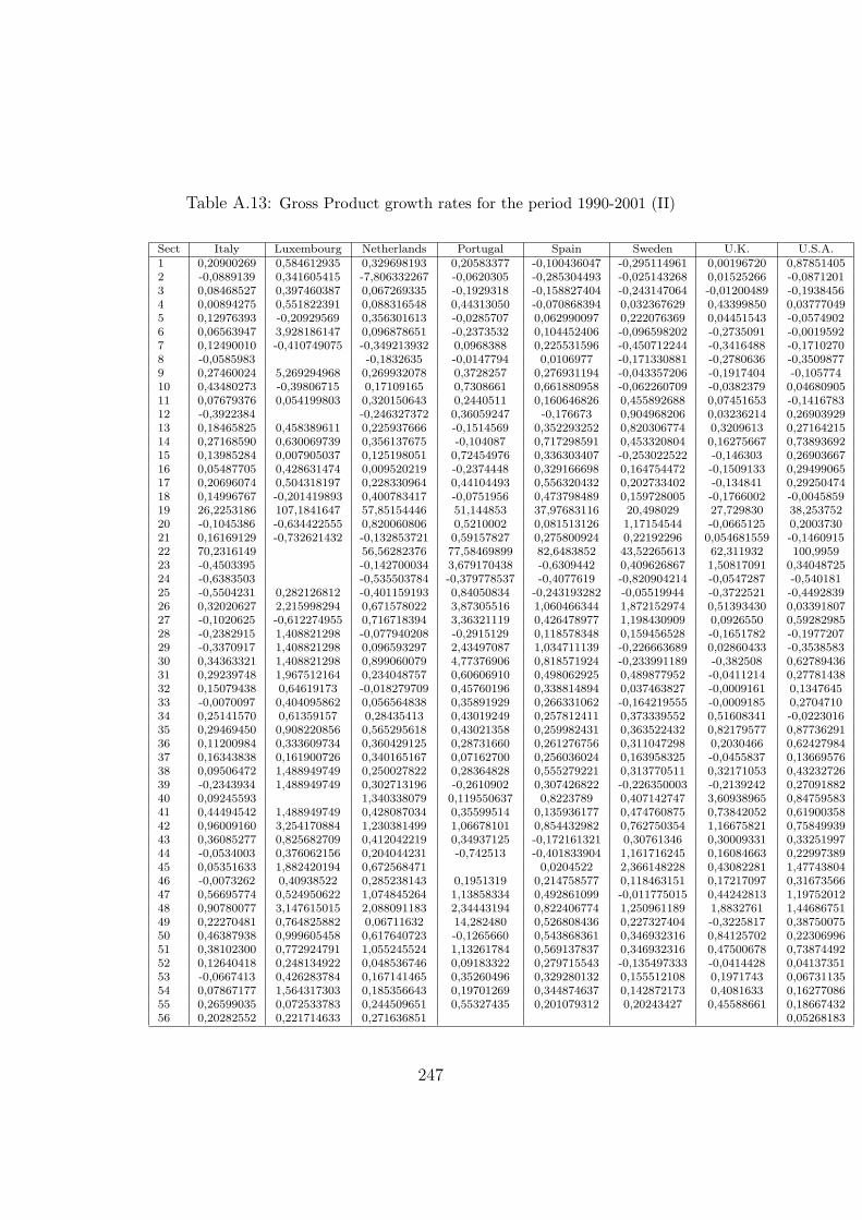
Table A.13: Gross Product growth rates for the period 1990-2001 (II)
Sect Italy Luxembourg Netherlands Portugal Spain Sweden U.K. U.S.A.1 0,20900269 0,584612935 0,329698193 0,20583377 -0,100436047 -0,295114961 0,00196720 0,878514052 -0,0889139 0,341605415 -7,806332267 -0,0620305 -0,285304493 -0,025143268 0,01525266 -0,08712013 0,08468527 0,397460387 0,067269335 -0,1929318 -0,158827404 -0,243147064 -0,01200489 -0,19384564 0,00894275 0,551822391 0,088316548 0,44313050 -0,070868394 0,032367629 0,43399850 0,037770495 0,12976393 -0,20929569 0,356301613 -0,0285707 0,062990097 0,222076369 0,04451543 -0,05749026 0,06563947 3,928186147 0,096878651 -0,2373532 0,104452406 -0,096598202 -0,2735091 -0,00195927 0,12490010 -0,410749075 -0,349213932 0,0968388 0,225531596 -0,450712244 -0,3416488 -0,17102708 -0,0585983 -0,1832635 -0,0147794 0,0106977 -0,171330881 -0,2780636 -0,35098779 0,27460024 5,269294968 0,269932078 0,3728257 0,276931194 -0,043357206 -0,1917404 -0,10577410 0,43480273 -0,39806715 0,17109165 0,7308661 0,661880958 -0,062260709 -0,0382379 0,0468090511 0,07679376 0,054199803 0,320150643 0,2440511 0,160646826 0,455892688 0,07451653 -0,141678312 -0,3922384 -0,246327372 0,36059247 -0,176673 0,904968206 0,03236214 0,2690392913 0,18465825 0,458389611 0,225937666 -0,1514569 0,352293252 0,820306774 0,3209613 0,2716421514 0,27168590 0,630069739 0,356137675 -0,104087 0,717298591 0,453320804 0,16275667 0,7389369215 0,13985284 0,007905037 0,125198051 0,72454976 0,336303407 -0,253022522 -0,146303 0,2690366716 0,05487705 0,428631474 0,009520219 -0,2374448 0,329166698 0,164754472 -0,1509133 0,2949906517 0,20696074 0,504318197 0,228330964 0,44104493 0,556320432 0,202733402 -0,134841 0,2925047418 0,14996767 -0,201419893 0,400783417 -0,0751956 0,473798489 0,159728005 -0,1766002 -0,004585919 26,2253186 107,1841647 57,85154446 51,144853 37,97683116 20,498029 27,729830 38,25375220 -0,1045386 -0,634422555 0,820060806 0,5210002 0,081513126 1,17154544 -0,0665125 0,200373021 0,16169129 -0,732621432 -0,132853721 0,59157827 0,275800924 0,22192296 0,054681559 -0,146091522 70,2316149 56,56282376 77,58469899 82,6483852 43,52265613 62,311932 100,995923 -0,4503395 -0,142700034 3,679170438 -0,6309442 0,409626867 1,50817091 0,3404872524 -0,6383503 -0,535503784 -0,379778537 -0,4077619 -0,820904214 -0,0547287 -0,54018125 -0,5504231 0,282126812 -0,401159193 0,84050834 -0,243193282 -0,05519944 -0,3722521 -0,449283926 0,32020627 2,215998294 0,671578022 3,87305516 1,060466344 1,872152974 0,51393430 0,0339180727 -0,1020625 -0,612274955 0,716718394 3,36321119 0,426478977 1,198430909 0,0926550 0,5928298528 -0,2382915 1,408821298 -0,077940208 -0,2915129 0,118578348 0,159456528 -0,1651782 -0,197720729 -0,3370917 1,408821298 0,096593297 2,43497087 1,034711139 -0,226663689 0,02860433 -0,353858330 0,34363321 1,408821298 0,899060079 4,77376906 0,818571924 -0,233991189 -0,382508 0,6278943631 0,29239748 1,967512164 0,234048757 0,60606910 0,498062925 0,489877952 -0,0411214 0,2778143832 0,15079438 0,64619173 -0,018279709 0,45760196 0,338814894 0,037463827 -0,0009161 0,134764533 -0,0070097 0,404095862 0,056564838 0,35891929 0,266331062 -0,164219555 -0,0009185 0,270471034 0,25141570 0,61359157 0,28435413 0,43019249 0,257812411 0,373339552 0,51608341 -0,022301635 0,29469450 0,908220856 0,565295618 0,43021358 0,259982431 0,363522432 0,82179577 0,8773629136 0,11200984 0,333609734 0,360429125 0,28731660 0,261276756 0,311047298 0,2030466 0,6242798437 0,16343838 0,161900726 0,340165167 0,07162700 0,256036024 0,163958325 -0,0455837 0,1366957638 0,09506472 1,488949749 0,250027822 0,28364828 0,555279221 0,313770511 0,32171053 0,4323272639 -0,2343934 1,488949749 0,302713196 -0,2610902 0,307426822 -0,226350003 -0,2139242 0,2709188240 0,09245593 1,340338079 0,119550637 0,8223789 0,407142747 3,60938965 0,8475958341 0,44494542 1,488949749 0,428087034 0,35599514 0,135936177 0,474760875 0,73842052 0,6190035842 0,96009160 3,254170884 1,230381499 1,06678101 0,854432982 0,762750354 1,16675821 0,7584993943 0,36085277 0,825682709 0,412042219 0,34937125 -0,172161321 0,30761346 0,30009331 0,3325199744 -0,0534003 0,376062156 0,204044231 -0,742513 -0,401833904 1,161716245 0,16084663 0,2299738945 0,05351633 1,882420194 0,672568471 0,0204522 2,366148228 0,43082281 1,4774380446 -0,0073262 0,40938522 0,285238143 0,1951319 0,214758577 0,118463151 0,17217097 0,3167356647 0,56695774 0,524950622 1,074845264 1,13858334 0,492861099 -0,011775015 0,44242813 1,1975201248 0,90780077 3,147615015 2,088091183 2,34443194 0,822406774 1,250961189 1,8832761 1,4468675149 0,22270481 0,764825882 0,06711632 14,282480 0,526808436 0,227327404 -0,3225817 0,3875007550 0,46387938 0,999605458 0,617640723 -0,1265660 0,543868361 0,346932316 0,84125702 0,2230699651 0,38102300 0,772924791 1,055245524 1,13261784 0,569137837 0,346932316 0,47500678 0,7387449252 0,12640418 0,248134922 0,048536746 0,09183322 0,279715543 -0,135497333 -0,0414428 0,0413735153 -0,0667413 0,426283784 0,167141465 0,35260496 0,329280132 0,155512108 0,1971743 0,0673113554 0,07867177 1,564317303 0,185356643 0,19701269 0,344874637 0,142872173 0,4081633 0,1627708655 0,26599035 0,072533783 0,244509651 0,55327435 0,201079312 0,20243427 0,45588661 0,1866743256 0,20282552 0,221714633 0,271636851 0,05268183
247

248
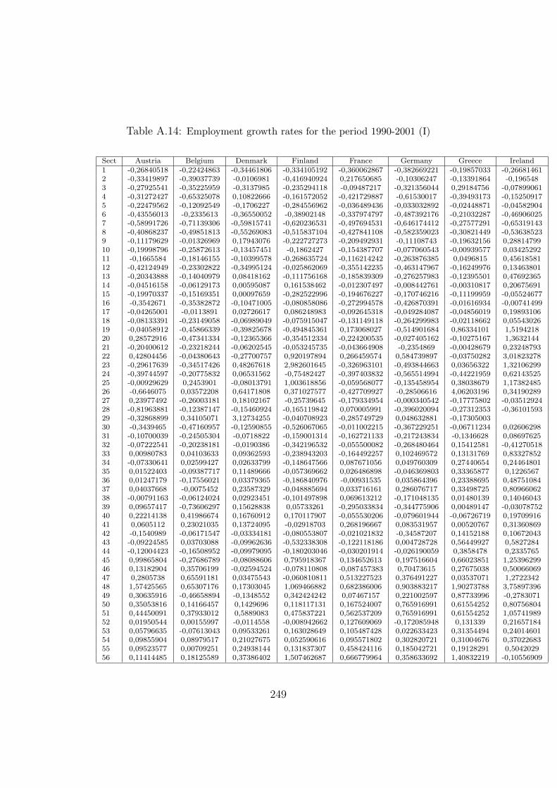
Table A.14: Employment growth rates for the period 1990-2001 (I)
Sect Austria Belgium Denmark Finland France Germany Greece Ireland1 -0,26840518 -0,22424863 -0,34461806 -0,334105192 -0,360062867 -0,382669221 -0,19857033 -0,266814612 -0,33419897 -0,39037739 -0,0106981 -0,416940924 0,217650685 -0,10306247 -0,13391864 -0,1965483 -0,27925541 -0,35225959 -0,3137985 -0,235294118 -0,09487217 -0,321356044 0,29184756 -0,078990614 -0,31272427 -0,65325078 0,10822666 -0,161572052 -0,421729887 -0,61530017 -0,39493173 -0,152509175 -0,22479562 -0,12092549 -0,1706227 -0,284556962 -0,036489436 -0,033032892 -0,02448871 -0,045829046 -0,43556013 -0,2335613 -0,36550052 -0,38902148 -0,337974797 -0,487392176 -0,21032287 -0,469060257 -0,58991726 -0,71139306 -0,59815741 -0,620236531 -0,497694531 -0,646174412 -0,27577291 -0,653191438 -0,40868237 -0,49851813 -0,55269083 -0,515837104 -0,427841108 -0,582359023 -0,30821449 -0,536385239 -0,11179629 -0,01326969 0,17943076 -0,222727273 -0,209492931 -0,11108743 -0,19632156 0,2881479910 -0,19998796 -0,25872613 -0,13457451 -0,1862427 -0,154387707 -0,077060543 -0,00939577 0,0342529211 -0,1665584 -0,18146155 -0,10399578 -0,268635724 -0,116214242 -0,263876385 0,0496815 0,4561858112 -0,42124949 -0,23302822 -0,34995124 -0,025862069 -0,355142235 -0,463147967 -0,16249976 0,1346380113 -0,20343888 -0,14040979 0,08418162 -0,111756168 -0,185839309 -0,276257983 -0,12395501 0,4769236514 -0,04516158 -0,06129173 0,00595087 0,161538462 -0,012307497 -0,008442761 -0,00310817 0,2067569115 -0,19970337 -0,15169351 0,00097659 -0,282522996 -0,194676227 -0,170746216 -0,11199959 -0,0552467716 -0,3542671 -0,35382872 -0,10471005 -0,080858086 -0,272994578 -0,426870391 -0,01616934 -0,0074149917 -0,04265001 -0,0113891 0,02726617 0,086248983 -0,092645318 -0,049284087 -0,04856019 0,1989310618 -0,08133391 -0,23149058 -0,06989049 -0,075915047 -0,131149118 -0,264299983 -0,02118662 0,0554302619 -0,04058912 -0,45866339 -0,39825678 -0,494845361 0,173068027 -0,514901684 0,86334101 1,519421820 0,28572916 -0,47341334 -0,12365366 -0,354512334 -0,224200535 -0,027405162 -0,10275167 1,363214421 -0,20400612 -0,23218244 -0,06202545 -0,053245735 -0,043664908 -0,2354869 -0,00428679 0,2324879322 0,42804456 -0,04380643 -0,27700757 0,920197894 0,266459574 0,584739897 -0,03750282 3,0182327823 -0,29617639 -0,34517426 0,48267618 2,982601645 -0,326963101 -0,493844663 0,03656322 1,3210629924 -0,39744597 -0,20775832 0,06531562 -0,75482427 -0,397403832 -0,565514994 -0,44221959 0,6214352525 -0,00929629 0,2453901 -0,08013791 1,003618856 -0,059568077 -0,135458954 0,38038679 1,1738248526 -0,6646075 0,03572208 0,64171808 0,371027577 -0,427709927 -0,28506616 4,06203196 0,3419028927 0,23977492 -0,26003181 0,18102167 -0,25739645 -0,179334954 -0,000340542 -0,17775802 -0,0351292428 -0,81963881 -0,12387147 -0,15460924 -0,165119842 0,070005991 -0,396020094 -0,27312353 -0,3610159329 -0,32868899 0,34105071 3,12734255 -0,040708923 -0,285749729 0,048632881 -0,1730500330 -0,3439465 -0,47160957 -0,12590855 -0,526067065 -0,011002215 -0,367229251 -0,06711234 0,0260629831 -0,10700039 -0,24505304 -0,0718822 -0,159001314 -0,162721133 -0,217243834 -0,1346628 0,0869762532 -0,07222541 -0,20238181 -0,0190386 -0,342196532 -0,055500082 -0,268480464 0,15412581 -0,4127051833 0,00980783 0,04103633 0,09362593 -0,238943203 -0,164492257 0,102469572 0,13131769 0,8332785234 -0,07330641 0,02599427 0,02633799 -0,148647566 0,087671056 0,049760309 0,27440654 0,2446480135 0,01522403 -0,09387717 0,11489666 -0,057369662 0,026486898 -0,046369803 0,33365877 0,122656736 0,01247179 -0,17556021 0,03379365 -0,186840976 -0,00931535 0,035864396 0,23388695 0,4875108437 0,04037668 -0,0075452 0,23587329 -0,048885694 0,033716161 0,286076717 0,33498725 0,8096606238 -0,00791163 -0,06124024 0,02923451 -0,101497898 0,069613212 -0,171048135 0,01480139 0,1404604339 0,09657417 -0,73606297 0,15628838 0,05733261 -0,295033834 -0,344775906 0,00489147 -0,0307875240 0,22214138 0,41986674 0,16760912 0,170117907 -0,055530206 -0,079601944 -0,06726719 0,1970991641 0,0605112 0,23021035 0,13724095 -0,02918703 0,268196667 0,083531957 0,00520767 0,3136086942 -0,1540989 -0,06171547 -0,03334181 -0,080553807 -0,021021832 -0,34587207 0,14152188 0,1067204343 -0,09224585 0,03703088 -0,09962636 -0,532338308 -0,122118186 0,004728728 0,56449927 0,582728444 -0,12004423 -0,16508952 -0,09979095 -0,180203046 -0,030201914 -0,026190059 0,3858478 0,233576545 0,99865804 -0,27686789 -0,08088606 0,795918367 0,134652613 0,197516604 0,66023851 1,2539629946 0,13182904 0,35706199 -0,02594524 -0,078110808 -0,087457383 0,70473615 0,27675038 0,5006606947 0,2805738 0,65591181 0,03475543 -0,060810811 0,513227523 0,376491227 0,03537071 1,272234248 1,57425565 0,65307176 0,17303045 1,069466882 0,682386006 0,903883217 1,90273788 3,7589739649 0,30635916 -0,46658894 -0,1348552 0,342424242 0,07467157 0,221002597 0,87733996 -0,278307150 0,35053816 0,14166457 0,1429696 0,118117131 0,167524007 0,765916991 0,61554252 0,8075680451 0,44450091 0,37933012 0,5889083 0,475837221 0,562537209 0,765916991 0,61554252 1,0574198952 0,01950544 0,00155997 -0,0114558 -0,008942662 0,127609069 -0,172085948 0,131339 0,2165718453 0,05796635 -0,07613043 0,09533261 0,163028649 0,105487428 0,022633423 0,31354494 0,2401460154 0,09855904 0,08979517 0,21027675 0,052590616 0,095571802 0,302820721 0,31004676 0,3702268355 0,09523577 0,00709251 0,24938144 0,131837307 0,458424116 0,185042721 0,19128291 0,504202956 0,11414485 0,18125589 0,37386402 1,507462687 0,666779964 0,358633692 1,40832219 -0,10556909
249

250
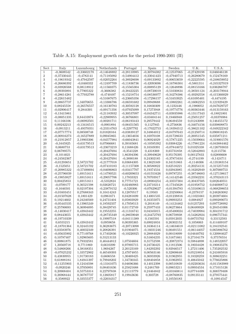
Table A.15: Employment growth rates for the period 1990-2001 (II)
Sect Italy Luxembourg Netherlands Portugal Spain Sweden U.K. U.S.A.1 -0,3608542 -0,33602178 -0,14648882 -0,28110985 -0,30794382 -0,12537065 -0,27429198 0,0460461382 -0,37330445 -0,4782141 -0,71185092 -0,54904412 -0,33041423 -0,47940713 -0,26280679 0,1524781693 -0,19619342 -0,47942597 -0,02052264 -0,38928698 -0,09133892 -0,00653659 -0,22225595 -0,2486590524 -0,26686392 -0,0460332 -0,12497709 -0,11836736 -0,42093696 -0,16786304 -0,5801314 -0,2453270195 -0,03926568 0,08118912 -0,11560375 -0,15565304 -0,00895129 -0,12648896 -0,08153166 0,0362667876 -0,09393891 0,77905322 -0,3606382 -0,38422225 -0,08720019 -0,51030834 -0,38501124 -0,2031789447 -0,28614281 -0,77932788 -0,4740497 -0,15218754 -0,08536977 -0,34278386 -0,49292558 -0,4153600298 -0,22615482 -0,51087675 -0,23605356 -0,17296157 -0,51653925 -0,61095401 -0,44741959 -0,08657737 1,34070655 -0,13306786 -0,06591682 0,09949688 -0,10802261 -0,16062253 0,12192942910 0,08245558 -0,26576557 -0,16130783 -0,30592128 0,16830309 -0,1232446 -0,1980052 -0,04762972711 -0,02906417 0,2844301 -0,09171356 -0,07925099 0,17273948 -0,19774776 -0,00363446 -0,01315916312 -0,13415861 -0,21183932 -0,30537097 -0,04342711 -0,03935986 -0,13117343 -0,1882180113 -0,08051335 0,84410974 -0,22909955 -0,36766801 -0,03404144 0,19460948 -0,25051257 -0,0337698414 0,11166106 -0,06992501 -0,00201711 -0,06193443 0,29579442 0,06494559 0,01243098 0,14645517215 0,00242213 -0,13416515 -0,0901894 -0,06451565 0,1127945 -0,2756836 -0,34074156 0,03980887316 -0,0913211 -0,49370351 -0,23314763 -0,2297792 -0,17022753 -0,18394512 -0,38621102 -0,04922234217 -0,07717774 0,08508748 0,01820164 -0,03839127 0,34864012 -0,04797643 -0,21250714 0,09081824518 -0,00916273 -0,16527889 0,09045865 -0,13654656 0,16970108 -0,01728633 -0,26951545 0,03587121119 -0,21912857 2,19903306 -0,04577984 -0,66043841 0,06924029 -0,57871225 -0,15039664 -0,31900157620 -0,3445925 -0,63179513 0,07066681 0,39165681 -0,10595392 0,03084226 -0,17981224 -0,04388446221 0,0680753 -0,63179513 -0,23673219 0,11688426 0,10349391 -0,07844672 0,01025338 -0,12679383322 0,06789575 -0,20427694 -0,3541228 0,4318369 0,65731858 -0,52042883 0,211575623 -0,1014021 -0,20427694 1,86394396 -0,39949628 0,95176395 0,00127833 0,0289060824 -0,24562367 -0,20427694 -0,3890188 0,24302185 -0,37871634 -0,2744199 -0,142471125 -0,01293651 2,58721702 -0,21777018 0,03684305 0,13625349 0,34151863 -0,1148306 -0,13538315426 -0,1525051 2,58721702 -0,07410183 -0,11157308 0,30580822 0,62516221 -0,20254131 -0,31525710327 -0,20985322 -0,57490694 -0,04696863 -0,03417707 0,19374534 0,02943085 -0,16202949 0,30700075328 -0,25796039 1,69151611 -0,14790521 -0,60209653 -0,01553426 0,09787255 -0,38748683 -0,12713861729 -0,19053827 1,69151611 -0,29057706 1,17833321 0,70703917 -0,14142546 -0,23562231 -0,37024311530 0,00425853 1,69151611 -0,5352824 0,77751721 -0,08904254 -0,33557304 -0,30437505 0,68264055131 -0,0709177 0,36521598 0,02620721 0,02460983 0,23710214 -0,17345628 -0,01958752 0,04690871232 -0,1646501 0,02197304 -0,23879152 -0,520306 -0,07629627 -0,01394783 -0,53169613 -0,06829865333 -0,01603451 0,27688343 0,10414243 0,12870517 0,19503 -0,23250064 -0,2378157 0,24826308234 -0,01507628 0,1801429 0,0961671 0,04281699 0,14001535 -0,01238816 -0,11021661 0,20397460435 0,19214602 0,24240569 0,24731404 0,05803929 0,16355075 0,09093253 0,0084927 0,09928907336 -0,05445535 0,13965249 0,18592337 0,17058513 0,2018149 -0,14124462 0,01257293 0,09772899237 0,25780693 0,36994095 0,38429745 0,01172749 0,25977433 0,06273664 0,06489928 0,20454100638 -0,14030417 0,43943442 0,19552255 -0,11316741 0,04345015 -0,05480024 -0,74039984 0,30419171239 0,08443655 0,43943442 -0,28735349 -0,28659048 -0,24472793 0,06759938 -0,54262924 0,09675734140 -0,19710339 0,19997518 -0,04111389 0,1565591 0,05912035 0,68755702 0,3315259341 0,6555215 0,43943442 0,0959658 0,00395365 0,69024834 0,26302152 0,1058063 0,41440910742 -0,18701364 0,32445192 0,36283675 -0,20713098 0,16364114 -0,14634619 -0,02111082 0,18419254143 0,03583976 0,40032349 0,20826391 0,01904075 -0,16031246 0,00491551 -0,06144057 0,06588676244 -0,05635992 0,77149768 0,17402836 -0,10226925 0,28884029 0,00418099 0,04640792 0,12098462745 0,10787407 1,92965605 0,55213133 0,51604235 0,51671661 0,27104179 0,3757655446 0,00861875 0,79332581 0,46444812 1,07504604 0,31752598 -0,20872374 0,59844898 0,14852205747 1,20569718 0,7711869 0,6610299 0,97995715 0,24736425 0,11812506 0,18034428 0,19083527648 0,54868266 4,38168351 1,9694267 2,20123169 1,84292292 0,92946517 1,27211406 1,73520253249 -0,07025232 1,33572902 0,46549393 2,47074855 0,00563146 0,32808648 0,05218854 0,24160591650 0,43830955 1,91730183 0,6606558 1,30469425 0,36933926 0,31962955 0,18320259 0,30863225151 0,61888184 1,84941397 0,79948202 1,34730345 0,68404858 0,31962955 0,40645042 0,77662580652 -0,11255903 0,12416598 -0,13161075 0,04696366 0,14012398 0,00510839 -0,02203634 -0,01158398953 -0,0920246 0,37050891 0,08401636 0,25821688 0,2481769 0,09653211 0,09934534 0,17101512654 0,20908404 0,55753314 0,22797838 0,21115779 0,24464842 -0,03160814 0,07744499 0,30857940855 0,26968444 0,36787737 0,12605817 0,19943636 0,303728 -0,08760835 0,09135141 0,27957544156 0,3580922 0,33555377 -0,22034317 3,10550183 -0,10914547
251

252

Appendix B
Mathematical Appendix toChapter 5
This appendix aims to detail some of the intermediate manipulations usedfor the presentation of the model. We will then explicit here the computationof the balance of payment constraint and the path allowing us to deduce theexpressions for the GDP growth rate as the expression for GDP.
B.1 The computation of the balance of pay-
ment constraint
Let us first consider Xc,t as the total exports of the domestic country:
Xc,t = (Yw,t)αjzc,t
It’s growth rate can then be expressed as follows:
∆Xc,t
Xc,t−1
= αc∆Yw,t
Yw,t−1
+∆zc,t
zc,t−1
The same procedure can be applied for imports. Hence starting from
Mc,t = (Yc,t)βc(1− zc,t)
It’s growth rate can then be expressed as follows:
∆Mc,t
Mc,t−1
= βc∆Yc,t
Yc,t−1
+∆(1− zc,t)
(1− zc,t−1)
Applying some minor manipulation this expression can be re-written as:
∆Mc,t
Mc,t−1
= βc∆Yc,t
Yc,t−1
− ∆zc,t
zc,t−1
zc,t−1
1− zc,t−1
253
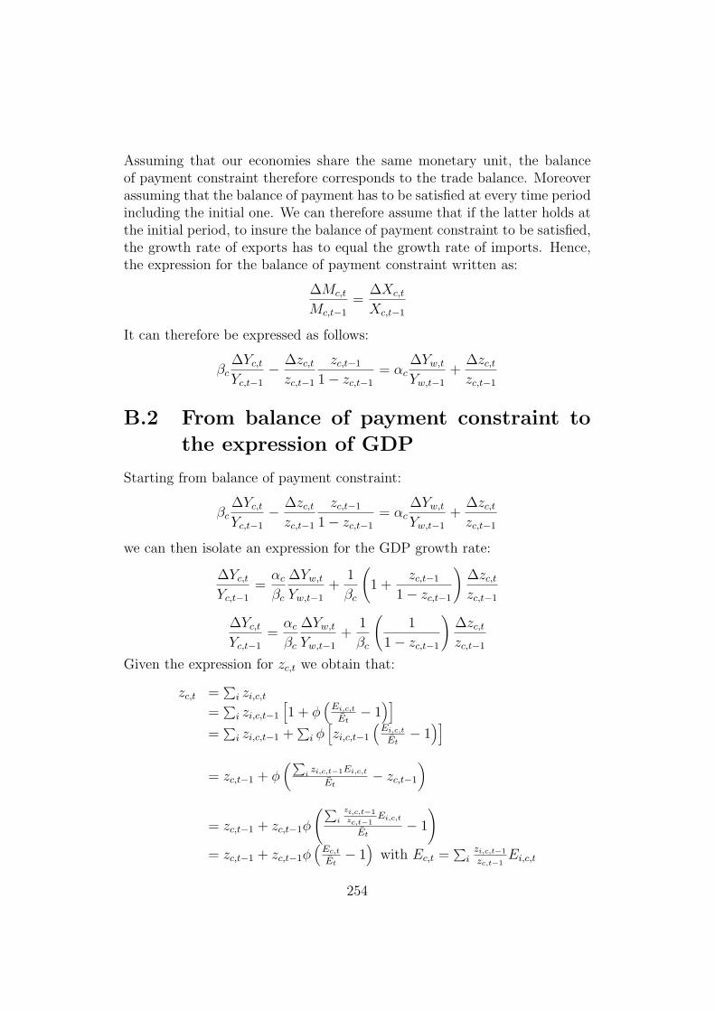
Assuming that our economies share the same monetary unit, the balanceof payment constraint therefore corresponds to the trade balance. Moreoverassuming that the balance of payment has to be satisfied at every time periodincluding the initial one. We can therefore assume that if the latter holds atthe initial period, to insure the balance of payment constraint to be satisfied,the growth rate of exports has to equal the growth rate of imports. Hence,the expression for the balance of payment constraint written as:
∆Mc,t
Mc,t−1
=∆Xc,t
Xc,t−1
It can therefore be expressed as follows:
βc∆Yc,t
Yc,t−1
− ∆zc,t
zc,t−1
zc,t−1
1− zc,t−1
= αc∆Yw,t
Yw,t−1
+∆zc,t
zc,t−1
B.2 From balance of payment constraint to
the expression of GDP
Starting from balance of payment constraint:
βc∆Yc,t
Yc,t−1
− ∆zc,t
zc,t−1
zc,t−1
1− zc,t−1
= αc∆Yw,t
Yw,t−1
+∆zc,t
zc,t−1
we can then isolate an expression for the GDP growth rate:
∆Yc,t
Yc,t−1
=αc
βc
∆Yw,t
Yw,t−1
+1
βc
(1 +
zc,t−1
1− zc,t−1
)∆zc,t
zc,t−1
∆Yc,t
Yc,t−1
=αc
βc
∆Yw,t
Yw,t−1
+1
βc
(1
1− zc,t−1
)∆zc,t
zc,t−1
Given the expression for zc,t we obtain that:
zc,t =∑
i zi,c,t
=∑
i zi,c,t−1
[1 + φ
(Ei,c,t
Et− 1
)]=∑
i zi,c,t−1 +∑
i φ[zi,c,t−1
(Ei,c,t
Et− 1
)]
= zc,t−1 + φ(∑
izi,c,t−1Ei,c,t
Et− zc,t−1
)
= zc,t−1 + zc,t−1φ
(∑i
zi,c,t−1zc,t−1
Ei,c,t
Et− 1
)= zc,t−1 + zc,t−1φ
(Ec,t
Et− 1
)with Ec,t =
∑i
zi,c,t−1
zc,t−1Ei,c,t
254
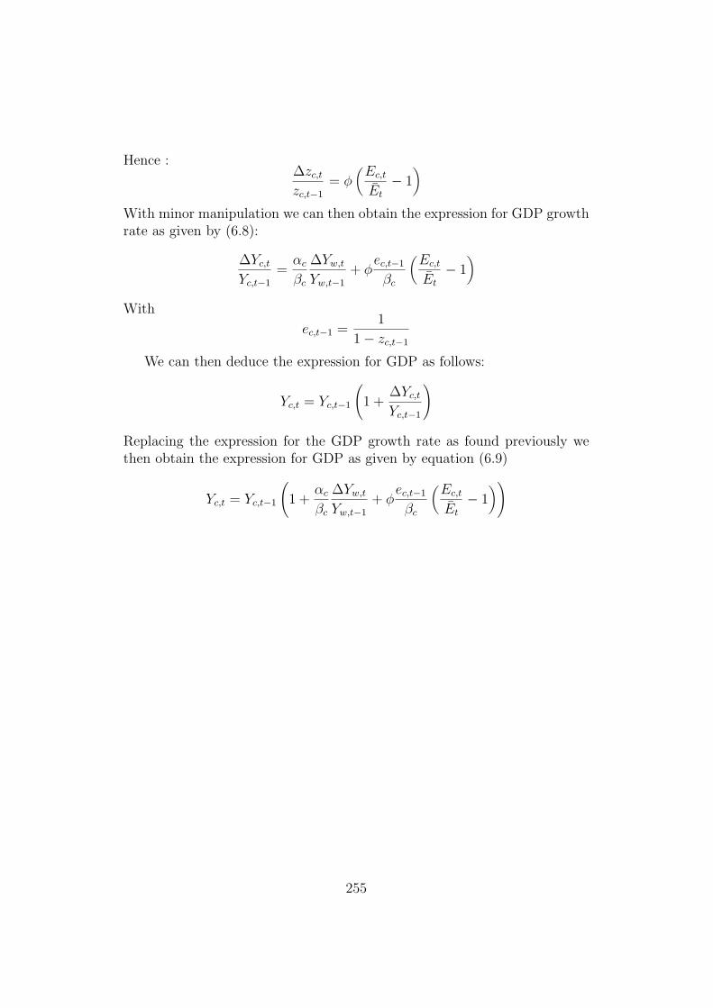
Hence :∆zc,t
zc,t−1
= φ(
Ec,t
Et
− 1)
With minor manipulation we can then obtain the expression for GDP growthrate as given by (6.8):
∆Yc,t
Yc,t−1
=αc
βc
∆Yw,t
Yw,t−1
+ φec,t−1
βc
(Ec,t
Et
− 1)
With
ec,t−1 =1
1− zc,t−1
We can then deduce the expression for GDP as follows:
Yc,t = Yc,t−1
(1 +
∆Yc,t
Yc,t−1
)
Replacing the expression for the GDP growth rate as found previously wethen obtain the expression for GDP as given by equation (6.9)
Yc,t = Yc,t−1
(1 +
αc
βc
∆Yw,t
Yw,t−1
+ φec,t−1
βc
(Ec,t
Et
− 1))
255

256
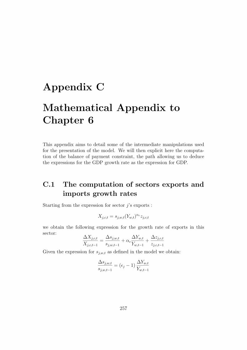
Appendix C
Mathematical Appendix toChapter 6
This appendix aims to detail some of the intermediate manipulations usedfor the presentation of the model. We will then explicit here the computa-tion of the balance of payment constraint, the path allowing us to deducethe expressions for the GDP growth rate as the expression for GDP.
C.1 The computation of sectors exports and
imports growth rates
Starting from the expression for sector j’s exports :
Xj,c,t = sj,w,t(Yw,t)αczj,c,t
we obtain the following expression for the growth rate of exports in thissector:
∆Xj,c,t
Xj,c,t−1
=∆sj,w,t
sj,w,t−1
+ αc∆Yw,t
Yw,t−1
+∆zj,c,t
zj,c,t−1
Given the expression for sj,w,t as defined in the model we obtain:
∆sj,w,t
sj,w,t−1
= (εj − 1)∆Yw,t
Yw,t−1
257
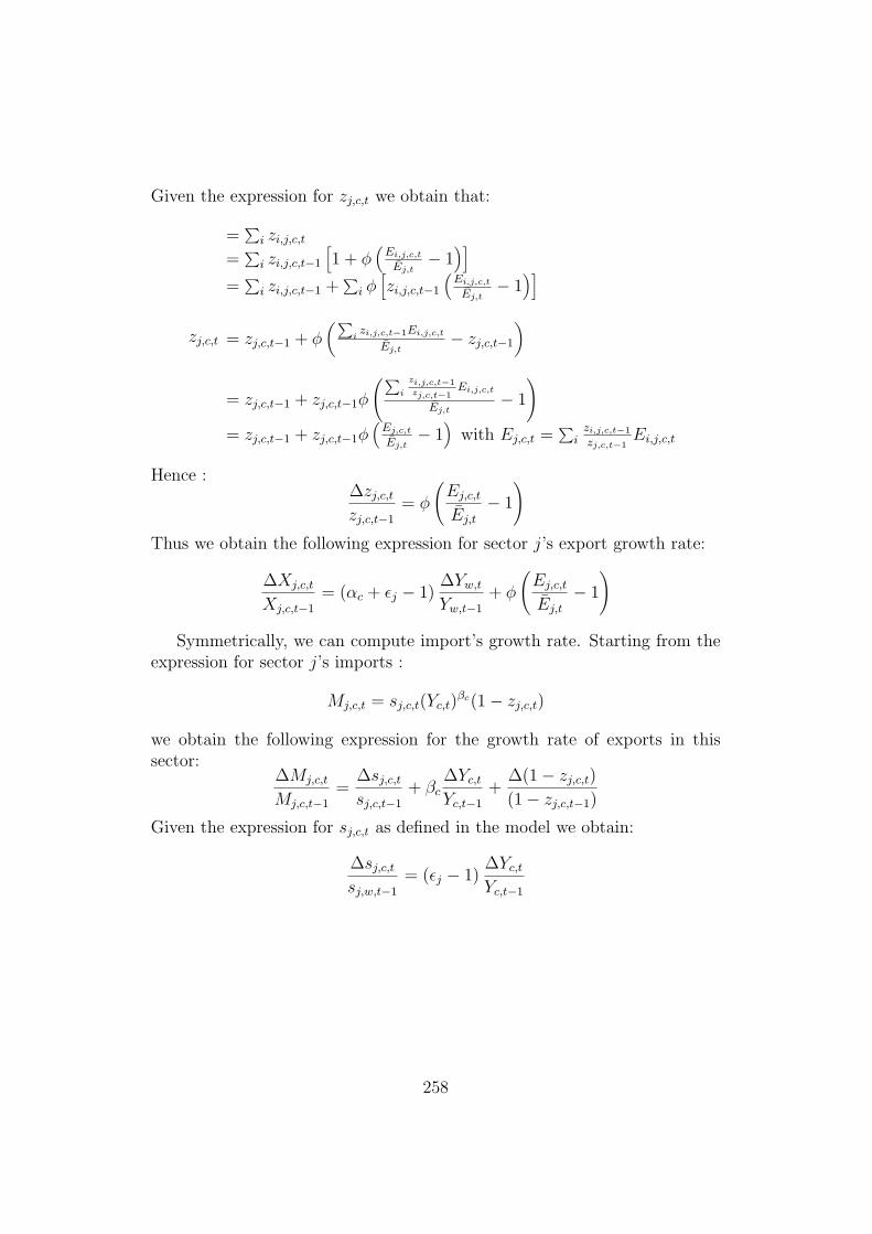
Given the expression for zj,c,t we obtain that:
zj,c,t
=∑
i zi,j,c,t
=∑
i zi,j,c,t−1
[1 + φ
(Ei,j,c,t
Ej,t− 1
)]=∑
i zi,j,c,t−1 +∑
i φ[zi,j,c,t−1
(Ei,j,c,t
Ej,t− 1
)]
= zj,c,t−1 + φ(∑
izi,j,c,t−1Ei,j,c,t
Ej,t− zj,c,t−1
)
= zj,c,t−1 + zj,c,t−1φ
(∑i
zi,j,c,t−1zj,c,t−1
Ei,j,c,t
Ej,t− 1
)= zj,c,t−1 + zj,c,t−1φ
(Ej,c,t
Ej,t− 1
)with Ej,c,t =
∑i
zi,j,c,t−1
zj,c,t−1Ei,j,c,t
Hence :∆zj,c,t
zj,c,t−1
= φ
(Ej,c,t
Ej,t
− 1
)Thus we obtain the following expression for sector j’s export growth rate:
∆Xj,c,t
Xj,c,t−1
= (αc + εj − 1)∆Yw,t
Yw,t−1
+ φ
(Ej,c,t
Ej,t
− 1
)
Symmetrically, we can compute import’s growth rate. Starting from theexpression for sector j’s imports :
Mj,c,t = sj,c,t(Yc,t)βc(1− zj,c,t)
we obtain the following expression for the growth rate of exports in thissector:
∆Mj,c,t
Mj,c,t−1
=∆sj,c,t
sj,c,t−1
+ βc∆Yc,t
Yc,t−1
+∆(1− zj,c,t)
(1− zj,c,t−1)
Given the expression for sj,c,t as defined in the model we obtain:
∆sj,c,t
sj,w,t−1
= (εj − 1)∆Yc,t
Yc,t−1
258
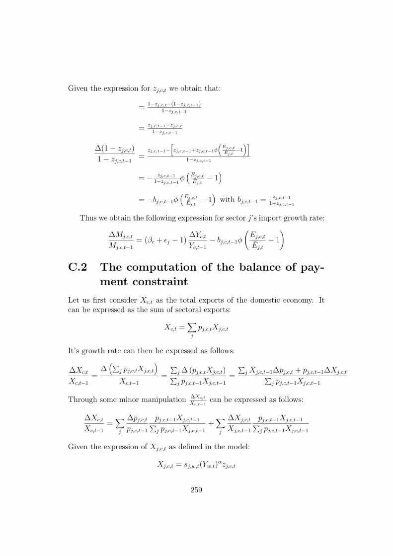
Given the expression for zj,c,t we obtain that:
∆(1− zj,c,t)
1− zj,c,t−1
= 1−zj,c,t−(1−zj,c,t−1)
1−zj,c,t−1
= zj,c,t−1−zj,c,t
1−zj,c,t−1
=zj,c,t−1−
[zj,c,t−1+zj,c,t−1φ
(Ej,c,tEj,t
−1
)]1−zj,c,t−1
= − zj,c,t−1
1−zj,c,t−1φ(
Ej,c,t
Ej,t− 1
)= −bj,c,t−1φ
(Ej,c,t
Ej,t− 1
)with bj,c,t−1 = zj,c,t−1
1−zj,c,t−1
Thus we obtain the following expression for sector j’s import growth rate:
∆Mj,c,t
Mj,c,t−1
= (βc + εj − 1)∆Yc,t
Yc,t−1
− bj,c,t−1φ
(Ej,c,t
Ej,t
− 1
)
C.2 The computation of the balance of pay-
ment constraint
Let us first consider Xc,t as the total exports of the domestic economy. Itcan be expressed as the sum of sectoral exports:
Xc,t =∑j
pj,c,tXj,c,t
It’s growth rate can then be expressed as follows:
∆Xc,t
Xc,t−1
=∆(∑
j pj,c,tXj,c,t
)Xc,t−1
=
∑j ∆ (pj,c,tXj,c,t)∑j pj,c,t−1Xj,c,t−1
=
∑j Xj,c,t−1∆pj,c,t + pj,c,t−1∆Xj,c,t∑
j pj,c,t−1Xj,c,t−1
Through some minor manipulation ∆Xc,t
Xc,t−1can be expressed as follows:
∆Xc,t
Xc,t−1
=∑j
∆pj,c,t
pj,c,t−1
pj,c,t−1Xj,c,t−1∑j pj,c,t−1Xj,c,t−1
+∑j
∆Xj,c,t
Xj,c,t−1
pj,c,t−1Xj,c,t−1∑j pj,c,t−1Xj,c,t−1
Given the expression of Xj,c,t as defined in the model:
Xj,c,t = sj,w,t(Yw,t)αzj,c,t
259
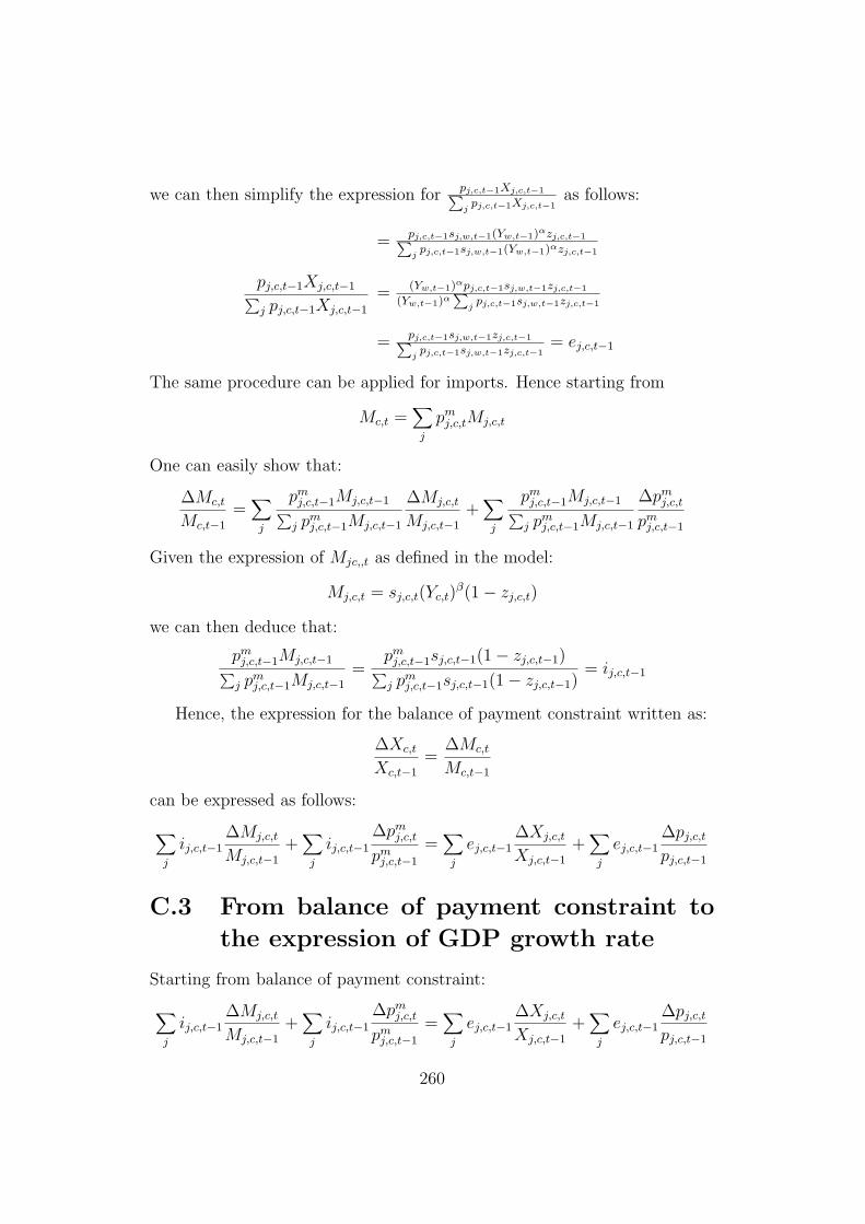
we can then simplify the expression for pj,c,t−1Xj,c,t−1∑j
pj,c,t−1Xj,c,t−1as follows:
pj,c,t−1Xj,c,t−1∑j pj,c,t−1Xj,c,t−1
= pj,c,t−1sj,w,t−1(Yw,t−1)αzj,c,t−1∑j
pj,c,t−1sj,w,t−1(Yw,t−1)αzj,c,t−1
= (Yw,t−1)αpj,c,t−1sj,w,t−1zj,c,t−1
(Yw,t−1)α∑
jpj,c,t−1sj,w,t−1zj,c,t−1
= pj,c,t−1sj,w,t−1zj,c,t−1∑j
pj,c,t−1sj,w,t−1zj,c,t−1= ej,c,t−1
The same procedure can be applied for imports. Hence starting from
Mc,t =∑j
pmj,c,tMj,c,t
One can easily show that:
∆Mc,t
Mc,t−1
=∑j
pmj,c,t−1Mj,c,t−1∑
j pmj,c,t−1Mj,c,t−1
∆Mj,c,t
Mj,c,t−1
+∑j
pmj,c,t−1Mj,c,t−1∑
j pmj,c,t−1Mj,c,t−1
∆pmj,c,t
pmj,c,t−1
Given the expression of Mjc,,t as defined in the model:
Mj,c,t = sj,c,t(Yc,t)β(1− zj,c,t)
we can then deduce that:
pmj,c,t−1Mj,c,t−1∑
j pmj,c,t−1Mj,c,t−1
=pm
j,c,t−1sj,c,t−1(1− zj,c,t−1)∑j pm
j,c,t−1sj,c,t−1(1− zj,c,t−1)= ij,c,t−1
Hence, the expression for the balance of payment constraint written as:
∆Xc,t
Xc,t−1
=∆Mc,t
Mc,t−1
can be expressed as follows:
∑j
ij,c,t−1∆Mj,c,t
Mj,c,t−1
+∑j
ij,c,t−1
∆pmj,c,t
pmj,c,t−1
=∑j
ej,c,t−1∆Xj,c,t
Xj,c,t−1
+∑j
ej,c,t−1∆pj,c,t
pj,c,t−1
C.3 From balance of payment constraint to
the expression of GDP growth rate
Starting from balance of payment constraint:
∑j
ij,c,t−1∆Mj,c,t
Mj,c,t−1
+∑j
ij,c,t−1
∆pmj,c,t
pmj,c,t−1
=∑j
ej,c,t−1∆Xj,c,t
Xj,c,t−1
+∑j
ej,c,t−1∆pj,c,t
pj,c,t−1
260
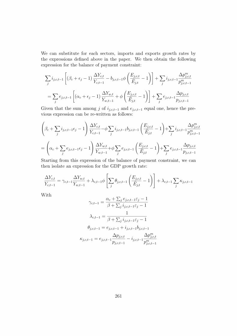
We can substitute for each sectors, imports and exports growth rates bythe expressions defined above in the paper. We then obtain the followingexpression for the balance of payment constraint:
∑j
ij,c,t−1
[(βc + εj − 1)
∆Yc,t
Yc,t−1
− bj,c,t−1φ
(Ej,c,t
Ej,t
− 1
)]+∑j
ij,c,t−1
∆pmj,c,t
pmj,c,t−1
=∑j
ej,c,t−1
[(αc + εj − 1)
∆Yw,t
Yw,t−1
+ φ
(Ej,c,t
Ej,t
− 1
)]+∑j
ej,c,t−1∆pj,c,t
pj,c,t−1
Given that the sum among j of ij,c,t−1 and ej,c,t−1 equal one, hence the pre-vious expression can be re-written as follows:βc +
∑j
ij,c,t−1εj − 1
∆Yc,t
Yc,t−1
−φ∑j
ij,c,t−1bj,c,t−1
(Ej,c,t
Ej,t
− 1
)+∑j
ij,c,t−1
∆pmj,c,t
pmj,c,t−1
=
αc +∑j
ej,c,t−1εj − 1
∆Yw,t
Yw,t−1
+φ∑j
ej,c,t−1
(Ej,c,t
Ej,t
− 1
)+∑j
ej,c,t−1∆pj,c,t
pj,c,t−1
Starting from this expression of the balance of payment constraint, we canthen isolate an expression for the GDP growth rate:
∆Yc,t
Yc,t−1
= γc,t−1∆Yw,t
Yw,t−1
+ λc,t−1φ
∑j
θj,c,t−1
(Ej,c,t
Ej,t
− 1
)+ λc,t−1
∑j
κj,c,t−1
With
γc,t−1 =αc +
∑j ej,c,t−1εj − 1
β +∑
j ij,c,t−1εj − 1
λc,t−1 =1
β +∑
j ij,c,t−1εj − 1
θj,c,t−1 = ej,c,t−1 + ij,c,t−1bj,c,t−1
κj,c,t−1 = ej,c,t−1∆pj,c,t
pj,c,t−1
− ij,c,t−1
∆pmj,c,t
pmj,c,t−1
261

262
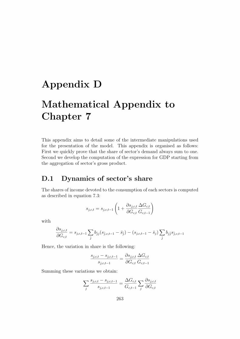
Appendix D
Mathematical Appendix toChapter 7
This appendix aims to detail some of the intermediate manipulations usedfor the presentation of the model. This appendix is organised as follows:First we quickly prove that the share of sector’s demand always sum to one.Second we develop the computation of the expression for GDP starting fromthe aggregation of sector’s gross product.
D.1 Dynamics of sector’s share
The shares of income devoted to the consumption of each sectors is computedas described in equation 7.3:
sj,c,t = sj,c,t−1
(1 +
∂sj,c,t
∂Gc,t
∆Gc,t
Gc,t−1
)
with
∂sj,c,t
∂Gc,t
= sj,c,t−1
∑j
bjj(sj,c,t−1 − sj)− (sj,c,t−1 − sj)∑j
bjjsj,c,t−1
Hence, the variation in share is the following:
sj,c,t − sj,c,t−1
sj,c,t−1
=∂sj,c,t
∂Gc,t
∆Gc,t
Gc,t−1
Summing these variations we obtain:
∑j
sj,c,t − sj,c,t−1
sj,c,t−1
=∆Gc,t
Gc,t−1
∑j
∂sj,c,t
∂Gc,t
263
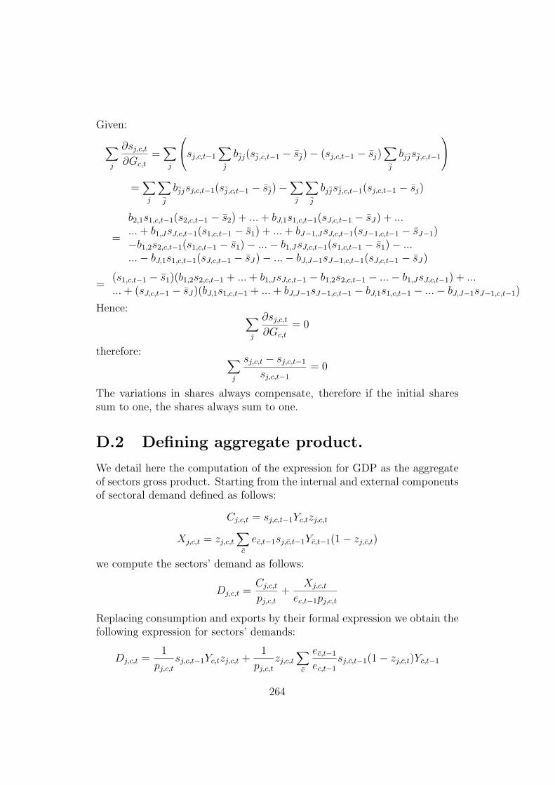
Given:
∑j
∂sj,c,t
∂Gc,t
=∑j
sj,c,t−1
∑j
bjj(sj,c,t−1 − sj)− (sj,c,t−1 − sj)∑j
bjjsj,c,t−1
=∑j
∑j
bjjsj,c,t−1(sj,c,t−1 − sj)−∑j
∑j
bjjsj,c,t−1(sj,c,t−1 − sj)
=
b2,1s1,c,t−1(s2,c,t−1 − s2) + ... + bJ,1s1,c,t−1(sJ,c,t−1 − sJ) + ...... + b1,JsJ,c,t−1(s1,c,t−1 − s1) + ... + bJ−1,JsJ,c,t−1(sJ−1,c,t−1 − sJ−1)−b1,2s2,c,t−1(s1,c,t−1 − s1)− ...− b1,JsJ,c,t−1(s1,c,t−1 − s1)− ......− bJ,1s1,c,t−1(sJ,c,t−1 − sJ)− ...− bJ,J−1sJ−1,c,t−1(sJ,c,t−1 − sJ)
=(s1,c,t−1 − s1)(b1,2s2,c,t−1 + ... + b1,JsJ,c,t−1 − b1,2s2,c,t−1 − ...− b1,JsJ,c,t−1) + ...... + (sJ,c,t−1 − sJ)(bJ,1s1,c,t−1 + ... + bJ,J−1sJ−1,c,t−1 − bJ,1s1,c,t−1 − ...− bJ,J−1sJ−1,c,t−1)
Hence: ∑j
∂sj,c,t
∂Gc,t
= 0
therefore: ∑j
sj,c,t − sj,c,t−1
sj,c,t−1
= 0
The variations in shares always compensate, therefore if the initial sharessum to one, the shares always sum to one.
D.2 Defining aggregate product.
We detail here the computation of the expression for GDP as the aggregateof sectors gross product. Starting from the internal and external componentsof sectoral demand defined as follows:
Cj,c,t = sj,c,t−1Yc,tzj,c,t
Xj,c,t = zj,c,t
∑c
ec,t−1sj,c,t−1Yc,t−1(1− zj,c,t)
we compute the sectors’ demand as follows:
Dj,c,t =Cj,c,t
pj,c,t
+Xj,c,t
ec,t−1pj,c,t
Replacing consumption and exports by their formal expression we obtain thefollowing expression for sectors’ demands:
Dj,c,t =1
pj,c,t
sj,c,t−1Yc,tzj,c,t +1
pj,c,t
zj,c,t
∑c
ec,t−1
ec,t−1
sj,c,t−1(1− zj,c,t)Yc,t−1
264
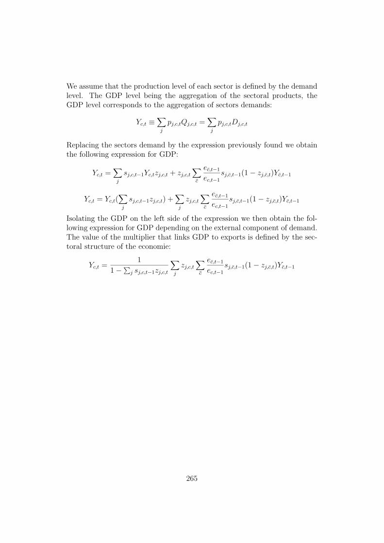
We assume that the production level of each sector is defined by the demandlevel. The GDP level being the aggregation of the sectoral products, theGDP level corresponds to the aggregation of sectors demands:
Yc,t ≡∑j
pj,c,tQj,c,t =∑j
pj,c,tDj,c,t
Replacing the sectors demand by the expression previously found we obtainthe following expression for GDP:
Yc,t =∑j
sj,c,t−1Yc,tzj,c,t + zj,c,t
∑c
ec,t−1
ec,t−1
sj,c,t−1(1− zj,c,t)Yc,t−1
Yc,t = Yc,t(∑j
sj,c,t−1zj,c,t) +∑j
zj,c,t
∑c
ec,t−1
ec,t−1
sj,c,t−1(1− zj,c,t)Yc,t−1
Isolating the GDP on the left side of the expression we then obtain the fol-lowing expression for GDP depending on the external component of demand.The value of the multiplier that links GDP to exports is defined by the sec-toral structure of the economie:
Yc,t =1
1−∑j sj,c,t−1zj,c,t
∑j
zj,c,t
∑c
ec,t−1
ec,t−1
sj,c,t−1(1− zj,c,t)Yc,t−1
265

266
List of Figures
3.1 Labour Productivity vs. GDP decades growth rates (Kaldor’s sam-ple) . . . . . . . . . . . . . . . . . . . . . . . . . . . . . . . . . 48
3.2 Employment vs. GDP decades growth rates (Kaldor’s sample) . . 503.3 Labour productivity vs. GDP decades growth rates (OECD sample) 533.4 Employment vs. GDP decades growth rates (OECD sample) . . . 553.5 Labour productivity vs. GDP decades growth rates (Entire sample) 583.6 Employment vs. GDP decades growth rates (Entire sample) . . . 61
4.1 Productivity level after 500 steps, ι vs. σ . . . . . . . . . . . . . 944.2 Productivity growth rate (50 first steps), ι vs. σ . . . . . . . . . . 954.3 Productivity growth rate (100 first steps), ι vs. σ . . . . . . . . . 954.4 Productivity growth rate (250 first steps), ι vs. σ . . . . . . . . . 964.5 Productivity level after 500 steps, ι vs. exogeneous demand growth 974.6 Productivity growth rate (50 first steps), ι vs. exogeneous demand
growth . . . . . . . . . . . . . . . . . . . . . . . . . . . . . . . 984.7 Productivity growth rate (100 first steps), ι vs. exogeneous de-
mand growth . . . . . . . . . . . . . . . . . . . . . . . . . . . . 994.8 Productivity growth rate (250 first steps), ι vs. exogeneous de-
mand growth . . . . . . . . . . . . . . . . . . . . . . . . . . . . 994.9 Productivity level after 500 steps, φ vs. χ . . . . . . . . . . . . . 1004.10 Productivity growth rate (50 first steps), φ vs. χ . . . . . . . . . 1014.11 Productivity growth rate (100 first steps),φ vs. χ . . . . . . . . . 1024.12 Productivity growth rate (250 first steps), φ vs. χ . . . . . . . . . 1024.13 Estimated Verdoorn coefficient (50 steps growth rates), ι vs. σ . . 1044.14 Student t for the Verdoorn coefficient (50 steps growth rates), ι vs. σ1054.15 Corrected R2 (50 steps growth rates), ι vs. σ . . . . . . . . . . . 1064.16 Estimated Verdoorn coefficient (50 steps growth rates), φ vs. χ . . 1074.17 Student t for the Verdoorn coefficient (50 steps growth rates), φ
vs. χ . . . . . . . . . . . . . . . . . . . . . . . . . . . . . . . . 1084.18 Corrected R2 (50 steps growth rates), φ vs. χ . . . . . . . . . . . 108
5.1 Differences in GDP growth rates with changes in γ and φ . . . . . 132
267
5.2 Differences in productivity growth rates with changes in γ and φ . 1335.3 Differences in GDP growth rates with heterogeneous αc and changes
in γ . . . . . . . . . . . . . . . . . . . . . . . . . . . . . . . . . 1345.4 Differences in GDP growth rates with heterogeneous αc. . . . . . . 1355.5 GDP growth rates with heterogeneous αc. . . . . . . . . . . . . . 1365.6 Differences in productivity growth rates with heterogeneous αc and
changes in γ . . . . . . . . . . . . . . . . . . . . . . . . . . . . 1365.7 Differences in GDP and productivity growth rates with heteroge-
neous βc . . . . . . . . . . . . . . . . . . . . . . . . . . . . . . 1375.8 Differences in GDP growth rates with heterogeneous σc and γ . . . 1385.9 Differences in GDP growth rates with heterogeneous σc . . . . . . 1385.10 GDP growth rates with heterogeneous σc. . . . . . . . . . . . . . 1395.11 Differences in productivity growth rates with heterogeneous σc . . 1405.12 Differences in GDP and productivity growth rates with changes in χ141
6.1 Specialisation levels and selection parameters (φ vs. ν) . . . . . . 1606.2 Specialisation dynamics with various values of ν . . . . . . . . . . 1616.3 Inter-sector differences in productivity growth rates and inter-sector
selection through wages . . . . . . . . . . . . . . . . . . . . . . 1626.4 Specialisation dynamics and price elasticity (φ) . . . . . . . . . . 1626.5 Specialisation levels with heterogeneous income elasticities (StdDev(εj)
vs. ν) . . . . . . . . . . . . . . . . . . . . . . . . . . . . . . . . 1636.6 Specialisation dynamics and heterogeneity in income elasticity . . 1646.7 Specialisation levels with heterogenous σj vs. ν . . . . . . . . . . 1656.8 Specialisation dynamics and heterogeneity in σj . . . . . . . . . 1656.9 Sectors’ share in total production (Average over the 5 economies) . 1666.10 Specialisation levels and the appropriability of spillovers (χ) . . . . 1676.11 Differences in GDP growth rates (Average over 500 steps) and
selection parameters (φ vs. ν) . . . . . . . . . . . . . . . . . . . 1686.12 Differences in GDP growth rates with various values of ν . . . . . 1696.13 Differences in GDP growth rates (Average over 500 steps) with
heterogenous income elasticities (StdDev(εj) vs. ν) . . . . . . . . 1706.14 Differences in GDP growth rates with heterogeneous income elas-
ticities . . . . . . . . . . . . . . . . . . . . . . . . . . . . . . . 1716.15 Differences in growth rates with heterogeneous σj . . . . . . . . . 1726.16 Differences in growth rates and appropriability of spillovers . . . . 172
7.1 Average inverse Herfindahl (Step 500), bjj vs. Std dev.(θ), ν = 0. . 1897.2 Coefficient of variation in real GDP growth rates, bjj vs. Std
dev.(θ), ν = 0. . . . . . . . . . . . . . . . . . . . . . . . . . . . 1907.3 Market shares (example) bjj = 0.5, Std dev.(θ) = 1.65, ν = 0. . . . 191
268
7.4 Sectors’ demand shares (example) bjj = 0,5, Std dev.(θ) = 1,65,ν = 0. . . . . . . . . . . . . . . . . . . . . . . . . . . . . . . . . 191
7.5 GDP growth rates (example run) bjj = 0.5, Std dev.(θ) = 1.65,ν = 0. . . . . . . . . . . . . . . . . . . . . . . . . . . . . . . . . 192
7.6 Coefficient of variation in GDP growth rates, bjj vs. Std dev.(θ),ν = 1. . . . . . . . . . . . . . . . . . . . . . . . . . . . . . . . . 193
7.7 Average inverse Herfindahl, bjj vs. Std dev.(θ), ν = 1. . . . . . . . 1937.8 Average Herfindahl index dynamics, bjj = 0.5, ν = 1. . . . . . . . 1947.9 GDP growth rates (example run) bjj = 0,5, Std dev.(θ) = 1,65,
ν = 1. . . . . . . . . . . . . . . . . . . . . . . . . . . . . . . . . 1967.10 Aggregate market shares (ex.) bjj=0.5, Std dev.(θ) = 1.65, ν = 1. . 1967.11 Sectors’ demand shares (ex.) bjj = 0.5, Std dev.(θ) = 1.65, ν = 1. 1977.12 Average inverse Herfindahl and demand shocks (Freq. vs. Std
Dev.) , ν = 0. . . . . . . . . . . . . . . . . . . . . . . . . . . . 1997.13 Coefficient of variation in GDP growth rates and demand shocks
(Freq. vs. Std Dev.) , ν = 0. . . . . . . . . . . . . . . . . . . . . 1997.14 GDP growth rates (example run) Freq. = 250, Std dev. = 1, ν = 0. 2007.15 Aggregate market shares (ex) Freq. = 250, Std dev. = 1, ν = 0. . 2017.16 Sectors’ demand shares (ex) Freq. = 250, Std dev. = 1, ν = 0. . . 2017.17 Coefficient of variation in GDP growth rates and demand shocks
(Freq. vs. Std Dev.) , ν = 1. . . . . . . . . . . . . . . . . . . . . 2027.18 Average inverse Herfindahl and demand shocks (Freq. vs. Std
Dev.) , ν = 1. . . . . . . . . . . . . . . . . . . . . . . . . . . . 203
269

270
List of Tables
3.1 Estimates for the Verdoorn specification with Kaldor’s sample . . 483.2 Differences in a2 across 5 decades (T-test) . . . . . . . . . . . . . 493.3 Estimates for the Kaldor specification using Kaldor’s sample . . . 513.4 T-test b1, b2 equal to 1 . . . . . . . . . . . . . . . . . . . . . . . 513.5 Kaldor (1966) and Pre-1974 OECD members samples of countries . 523.6 Estimates for the Verdoorn specification using the OECD sample . 533.7 Differences in a2 across time (T-test) . . . . . . . . . . . . . . . . 543.8 Estimates for the Kaldor specification using the OECD sample . . 553.9 T-test for b1, b2 equal to 1 . . . . . . . . . . . . . . . . . . . . . 563.10 Extended sample for the various periods . . . . . . . . . . . . . . 573.11 Estimates for the Verdoorn specification (Entire sample) . . . . . 603.12 Estimates for the Kaldor specification (Entire sample) . . . . . . . 633.13 List of sectors . . . . . . . . . . . . . . . . . . . . . . . . . . . 653.14 Kaldor-Verdoorn Law estimates (All Industry) 1980-1990 . . . . . 663.15 Sectoral estimations of Verdoorn’s specification (1980-1990) . . . . 673.16 Sectoral estimations of Kaldor’s specification (1980-1990) . . . . . 683.17 T-test for b2=1 (1980-1990) . . . . . . . . . . . . . . . . . . . . 693.18 T-test: Sector’s estimates differences with ‘All Industry’ (1980-1990) 713.19 Kaldor-Verdoorn Law estimates 1990-2000 (All Industry) . . . . . 723.20 Sectoral estimations of the Verdoorn specification (1990-2000) . . . 743.21 Sectoral estimations of the Kaldor specification (1990-2000) . . . . 753.22 T-test for b2=1 (1990-2000) . . . . . . . . . . . . . . . . . . . . 773.23 T-test: Sector’s estimates differences with ‘All Industry’ (1990-2000) 783.24 T-test: Differences among periods (1990-2000 vs. 1980-1990) . . . 80
4.1 Main Simulation Results . . . . . . . . . . . . . . . . . . . . . . 1094.2 Parameters settings (the values by default are in italic) . . . . . . 111
5.1 Main Simulation Results . . . . . . . . . . . . . . . . . . . . . . 1425.2 Key parameters settings (the values by default are in italic) . . . . 1445.3 Other parameters and initial conditions . . . . . . . . . . . . . . 145
271
6.1 Main Simulation Results . . . . . . . . . . . . . . . . . . . . . . 1736.2 Key parameters settings (the values by default are in italic) . . . . 1756.3 Other parameters and initial conditions . . . . . . . . . . . . . . 176
7.1 Main Simulation Results . . . . . . . . . . . . . . . . . . . . . . 2057.2 Key parameters settings . . . . . . . . . . . . . . . . . . . . . . 2067.3 Other parameters and initial conditions . . . . . . . . . . . . . . 207
A.1 Growth rates for the period 1950 - 1960 . . . . . . . . . . . . . . 230A.2 Growth rates for the period 1960 - 1970 . . . . . . . . . . . . . . 231A.3 Growth rates for the period 1970 - 1980 . . . . . . . . . . . . . . 232A.4 Growth rates for the period 1980 - 1990 . . . . . . . . . . . . . . 233A.5 Growth rates for the period 1990 - 2000 . . . . . . . . . . . . . . 234A.6 Total industry growth rates for the period 1980-1990 . . . . . . . 235A.7 Total industry growth rates for the period 1990-2001 . . . . . . . 235A.8 Gross Product growth rates for the period 1980-1990 (I) . . . . . . 237A.9 Gross Product growth rates for the period 1980-1990 (II) . . . . . 239A.10 Employment growth rates for the period 1980-1990 (I) . . . . . . 241A.11 Employment growth rates for the period 1980-1990 (II) . . . . . . 243A.12 Gross Product growth rates for the period 1990-2001 (I) . . . . . . 245A.13 Gross Product growth rates for the period 1990-2001 (II) . . . . . 247A.14 Employment growth rates for the period 1990-2001 (I) . . . . . . 249A.15 Employment growth rates for the period 1990-2001 (II) . . . . . . 251
272


