Essays on the Demand for Prescription Drugs
145
Essays on the Demand for Prescription Drugs By Niels Skipper A dissertation submitted to the Faculty of Social Sciences, Aarhus University in partial fulfilment of the requirements of the PhD degree in Economics and Management
Transcript of Essays on the Demand for Prescription Drugs

Essays on the Demand for Prescription Drugs
By Niels Skipper
A dissertation submitted to
the Faculty of Social Sciences, Aarhus University
in partial fulfilment of the requirements of
the PhD degree in
Economics and Management


Table of Contents
Preface 5
Summary
7
Summary in Danish (dansk resume) 10
Chapter 1 On Utilization and Stockpiling of Prescription Drugs when Co-payments Increase: Heterogeneity across Types of Drugs
13
Chapter 2 Price Sensitivity of Demand for Prescription Drugs: Exploiting a Regression Kink Design
59 Chapter 3 Income and the Use of Prescription Drugs for Near Retirement Individuals
107


5
Preface
This dissertation was written in the period August 2006 to July 2010 while I was enrolled as a PhD
student at the School of Economics and Management at Aarhus University. I would like to thank
the School for providing an excellent research environment and the possibility to attend numerous
conferences and courses.
I would like to thank my advisor, Michael Svarer, for always being available and offering
comments on my work. I would also like to thank my secondary advisor, Søren Leth-Petersen, for
his effort on the last chapter of the thesis. During the work on this dissertation, I have learnt a lot
from working with Søren Leth-Petersen, Marianne Simonsen and Lars Skipper, and I am deeply
thankful to all of them. Especially Marianne for always being kind to offer comments and advice on
every stage of my work. Also thanks to Lars for inspiring me to follow this academic path. In
addition, I would like to thank Jonas, Lasse, Mikkel, Maria, Rune, Torben and all the PhD students
at the School for offering a terrific working environment. I am grateful for meeting a very good
friend, Frank Steen Nielsen, with whom I had the great pleasure of sharing office for three and a
half years.
During my studies, I visited the Economics Department at the University of Maryland at College
Park, and I would like to thank the department for its hospitality.
Thanks to Birgitte Højklint Nielsen and Thomas Stephansen for excellent proofreading.
A very special thanks goes to Dyveke for being patient and understanding whenever conversations
at family dinners iterated around topics like endogeneity, forward-looking agents and regression
kink designs. Thank you for your love and support throughout the entire process. Finally, I would
like to thank the members of my family not already mentioned.
Niels Skipper
Aarhus, July 2010

6
The pre-defense was held on September 28th, 2010. I would like to thank the members of the
assessment committee, Paul Bingley, Tom Crossley and Helena Skyt Nielsen (chair) for their
insightful comments and suggestions. Some of the suggestions have already been incorporated, and
more will follow in the near future.
Niels Skipper
Aarhus, November 2010

7
Summary
This dissertation consists of three self-contained chapters on the demand for prescription drugs.
More specifically, the first two papers focus on how price responsive the demand for prescription
drugs is, and the third and last paper is on the relationship between income and the use of
prescription drugs.
It is a well-established fact that health care expenditures are growing rapidly in most countries in
the world, and that they are foreseen to do so in the future as well. Of these expenditures the
component that experiences the largest growth is that of prescription drugs. Given that most
developed countries provide some degree of government subsidies to prescription drugs
consumption, price and income elasticities of demand are important parameters for designing
optimal reimbursement schemes. The economics literature in the area is growing, but there is
considerable variation in the obtained estimates, which is possibly due to data limitations. That is,
in the existing studies the data used often stems from specific sub-groups of the population. The
papers in this thesis make use of data on prescription drug purchases for a 20 % random sample of
the entire Danish population over the period 1995 to 2003. The high quality of these data allows for
estimating the above-mentioned parameters for different sub-groups of the overall population, as
well as for different types of drugs, within a unifying framework that has not been seen before in
the literature.
The first chapter, “On Utilization and Stockpiling of Prescription Drugs when Co-payments
Increase: Heterogeneity across Types of Drugs”, uses variation in subsidy rates over time to identify
the price elasticity of demand. This is the typical approach used in the literature. However, I show
that using changes in subsidy rates over time may not be suitable for identifying price elasticities
when people have information about these subsidy changes. Normally, the data sets used in the
literature only have information on total drug spending or the like. Due to the degree of detail in the
Danish data, I show that people who consume drugs to maintain a chronic condition (insulin for
diabetics) react to these changes by stockpiling on their medications prior to the price increases.
That is, people foresee future price increases and plan their consumption by acquiring the drugs
while they can get them at low cost. This will lead the researcher to overestimate the associated
demand response of a price change. I also show that this stockpiling behavior is more pronounced
8
for the upper part of the income distribution among those in treatment with insulin. On the other
hand, this identification strategy is suitable for drugs that maintain transitory and non-chronic
conditions (penicillin to treat infections). The price elasticity for the non-chronic drugs is estimated
to be around -.2, with the lower part of the income distribution being more price elastic.
In the second chapter, “Price Sensitivity of Demand for Prescription Drugs: Exploiting a Regression
Kink Design” (co-authored with Marianne Simonsen and Lars Skipper), we estimate the demand
elasticity of prescription drugs using a regression kink design. Instead of using variation in co-
payments over time for identifying the price elasticity of demand, we directly exploit that
coinsurance payments decrease in a discontinuous fashion as consumption (on a yearly basis)
increases. The idea behind this identification strategy is very close to that of a regression
discontinuity design, which has been used extensively in the applied microeconometrics literature.
We are, however, to the best of our knowledge, among the very first to directly implement the
regression kink design. The basic idea is that there is no reason to think that individuals just above a
given kink point are different from individuals just below – except for the fact that the price faced
by individuals below the kink point decreases less with total consumption than for individuals
above the kink point. Comparing the propensity to purchase for individuals who are just above with
that for individuals who are just below kink points then allows us to identify price sensitivities. Our
results suggest that demand is inelastic; we find low average price responsiveness with a
corresponding price elasticity ranging from -0.09 to -0.25. Individuals with lower education and
income are, however, more responsive to the price, and the same is true for the elderly population.
Furthermore, essential drugs that surely prevent deterioration of health and prolong life have, as
expected, much lower associated average price sensitivity than the complementary set of drugs.
In the third and final chapter, “Income and the Use of Prescription Drugs for Near Retirement
Individuals” (co-authored with Søren Leth-Petersen), the objective is to estimate how demand for
prescription drugs varies with income for near retirement individuals. The focus is on near
retirement individuals because demand for prescription drugs increases dramatically from around
age 55, and because this group experiences considerable income variations around the point of
retirement. Estimating how prescription drug demand responds to income variations is complicated
by the fact that demand for drugs is likely to be related to the health capital which is generally
unobserved and can often at best only be proxied by including measures of self-reported health
when analyzing cross section data. Controlling for health capital is important because the level of

9
health capital tends to be related to marginal productivity, so that individuals with a higher level of
health capital also have a higher level of human capital. Therefore, comparing demand of
individuals with high income with that of individuals with low income in order to estimate Engle
curves is likely to (also) reflect selection effects. Moreover, the use of prescription drugs is likely to
be endogenous to the extent that consuming drugs improves health and thereby earnings capacity
and income. Another issue relates to the dynamic aspects of drug demand. We argue that it is
crucial to control for all of them when modeling the dependence of demand for prescription drugs
on income. In fact leaving out one of these elements from the analysis can lead to seriously biased
Engle curve estimates. The results show a strong relationship between income and the demand for
prescription drugs when estimated on a cross section. However, taking into account the dynamic
structure of demand as well as fixed factors controlling for individual specific levels of health
capital is very important in this context. Applying an appropriate panel data model weakens this
relationship considerably. This suggests that Engle curve relationships estimated off cross section
data may lead to biased estimates of the Engle curve relationship and that caution is warranted when
giving such estimates a behavioral interpretation, i.e., as an estimate of the demand response to a
change in income. However, the results in the paper still point to the fact that reforms affecting
income, for example reforms of the public pension provision, will affect the demand for
prescription drugs.

10
Summary in Danish (dansk resume)
Denne afhandling består af tre selvstændige kapitler, der omhandler efterspørgslen efter
receptpligtig medicin. De to første kapitler fokuserer på sammenhængen mellem efterspørgslen
efter receptpligtig medicin og prisen på denne. Det tredje og sidste kapitel fokuserer på
sammenhængen mellem indkomst og brugen af receptpligtig medicin.
Det er et velkendt faktum, at der er sket en stor vækst i sundhedsudgifterne i stort set alle verdens
lande, og at disse udgifter antages at vokse yderligere fremover. Et af de elementer af
sundhedsudgifterne, der vokser allermest, er udgifterne til receptpligtig medicin. De fleste
udviklede lande subsidierer i større eller mindre grad borgernes brug af receptpligtig medicin,
hvorfor viden om pris- og indkomstelasticiteter er vigtigt, når der skal designes tilskudssystemer
mv. Der er en voksende økonomisk litteratur på området, men der er en betydelig variation i de
estimater, der opnås, hvilket øjensynligt kan tilskrives mangel på data af en ordentlig kvalitet. I de
eksisterende studier inkluderer de anvendte datasæt oftest kun information om helt specifikke
befolkningsgrupper, hvilket gør det svært at sige noget om den generelle befolkning, endsige påvise
forskelle inden for det samme institutionelle regime. Fælles for kapitlerne i denne afhandling er, at
de gør brug af en tilfældig stikprøve på 20 % af hele den danske befolkning fra perioden 1995-2003
og disses køb af receptpligtig medicin. Sammenlignet med andre studier er disse data af meget høj
kvalitet, hvilket gør det muligt at estimere de førnævnte elasticitetesparametre for hele befolkningen
samt for forskellige sub-populationer. Endvidere er det også muligt at kortlægge prisresponset for
forskellige typer af lægemidler, alt sammen inden for det samme institutionelle regime.
Det første kapitel, ”On Utilization and Stockpiling of Prescription Drugs when Co-payments
Increase: Heterogeneity across Types of Drugs”, gør brug af ændringer i størrelsen af
medicintilskud over tid til at identificere efterspørgslens priselasticitet. Dette er den typiske strategi
inden for litteraturen. I kapitlet viser jeg, at dette kan give meget misvisende resultater, når
forbrugeren har informationer om kommende tilskudsændringer. I de datasæt, der har været brugt i
den eksisterende litteratur, har man oftest kun haft information om de samlede udgifter til
lægemidler eller lignende. Ved at gøre brug af de særligt detaljerede danske registerdata viser jeg, at
folk, der er i behandling for en kronisk lidelse (insulin til diabetikere), reagerer på stigende priser på
medicinen ved at hamstre. Det vil sige, at folk er forudseende og i stand til at planlægge deres

11
forbrug ved at anskaffe sig medicinen, så længe den er billig. Dette medfører, at man vil
overestimere prisfølsomheden ved en given ændring i prisen. Jeg viser også, at blandt dem, der er i
behandling med insulin, er hamstringen er mere udtalt hos den øverste del af indkomstfordelingen.
På den anden side er denne identifikationsstrategi passende, når man kigger på lægemidler til
transitoriske og ikke-kroniske tilstande (penicillin til behandling af infektioner). Priselasticiteten for
dette lægemiddel estimeres til at være ca. -0,2. Endvidere finder jeg, at den nederste del af
indkomstfordelingen er mere prissensitiv end den øverste.
I det andet kapitel, ”Price Sensitivity of Demand for Prescription Drugs: Exploiting a Regression
Kink Design” (skrevet med Marianne Simonsen og Lars Skipper), estimeres efterspørgslens
priselasticitet ved hjælp af et såkaldt regression kink design. I stedet for at gøre brug af
tilskudsændringer over tid, udnytter vi, at den individspecifikke egenbetaling falder diskontinuert i
det årlige forbrug. Denne identifikationsstrategi er meget lig et regression discontinuity design.
Sidstnævnte er allerede en meget udbredt identifikationsstrategi inden for den anvendte
mikroøkonometri. Det er dog vores bedste overbevisning, at vi er blandt de allerførste til direkte at
implementere et regression kink design. Idéen er, at individer, der er placeret lige under et givent
kink-punkt, ikke er forskellige fra individer, der ligger lige over et givent kink-punkt, udover at den
pris, førstnævnte står overfor, aftager mindre med totalforbruget. Således kan vi sammenligne
købstilbøjeligheden for individer, der ligger lige under og lige over et givent kink-punkt, og derved
identificere efterspørgslens priselasticitet. Vores resultater viser, at efterspørgslen efter receptpligtig
medicin er inelastisk med estimerede elasticiteter i intervallet -0.09 til -0.25. Vi finder, at
lavtuddannede samt folk med lav indkomst er mere prisfølsomme. Det samme gør sig gældende for
den ældre del af befolkningen. Ydermere finder vi, at efterspørgslen efter gruppen af lægemidler,
der med stor sikkerhed forebygger en forværring af helbredet og er livsforlængende, er betydeligt
mindre prisfølsom end den resterende gruppe af lægemidler.
I det tredje og sidste kapitel, ”Income and the Use of Prescription Drugs for Near Retirement
Individuals” (skrevet med Søren Leth-Petersen), estimerer vi, hvordan efterspørgslen efter
receptpligtige lægemidler varierer med indkomsten for folk, der er nær pensionsalderen. Vi
fokuserer netop på denne gruppe, da efterspørgslen efter receptpligtige lægemidler stiger kraftigt fra
55 års alderen, og da denne gruppe oplever en betydelig variation i indkomsten omkring
tilbagetrækningstidspunktet. Estimeringen af dette indkomstrespons er kompliceret af det faktum, at
efterspørgslen efter receptpligtig medicin sandsynligvis er relateret til et individs sundhedskapital,
12
der generelt er uobserverbart. Det er imidlertid vigtigt at kontrollere for denne sundhedskapital, da
denne vil være relateret til individets marginalproduktivitet, således at individer med et højt niveau
af sundhedskapital også har et højt niveau af humankapital. Derfor vil estimeringen af Engelkurver,
der blot sammenligner højindkomstindivider med lavindkomstindivider, også afspejle
selektionseffekter. Derudover er brugen af receptpligtige lægemidler sandsynligvis endogen i det
omfang, at brugen af lægemidler forbedrer helbredet og dermed indtjeningsmulighederne samt
indkomsten. Et andet element, der komplicerer problemstillingen, er det dynamiske aspekt af
efterspørgslen. Vi argumenterer for, at det er afgørende at kontrollere for ovenstående, når man skal
modellere efterspørgslen efter lægemidlers afhængighed af indkomsten. Faktisk kan udeladelse af ét
af disse elementer give anledning til en ikke ubetydelig bias i Engelkurveestimaterne. Vores
resultater viser, at der er en stærk sammenhæng mellem indkomsten og efterspørgslen efter
receptpligtig medicin, når denne estimeres på tværsnitsdata. Det at tage højde for efterspørgslens
dynamiske struktur, samt at kontrollere for den individspecifikke sundhedskapital, viser sig at være
meget vigtigt i denne sammenhæng. Når vi anvender en paneldatamodel, der favner alle de nævnte
komplikationer, reduceres indkomstsammenhængen betydeligt. Dette antyder, at
Engelkurvesammenhænge, der er estimeret på tværsnitsdata, kan være biased, og at man skal være
varsom med at tolke på disse. Resultaterne viser dog, at reformer, der påvirker indkomsten, f.eks.
reformer af pensionssystemet, vil påvirke efterspørgslen efter receptpligtig medicin.

13
CHAPTER 1
On Utilization and Stockpiling of Prescription Drugs when
Co-payments Increase:
Heterogeneity across Types of Drugs

14

15
On Utilization and Stockpiling of Prescription Drugs when
Co-payments Increase:
Heterogeneity across Types of Drugs
November 2010
Niels Skipper
School of Economics
and Management
Aarhus University
Abstract: This paper investigates prescription drug utilization changes following an exogenous shift in
consumer co-payment caused by a reform in the Danish subsidy scheme for the general public. Two
different types of medication are considered – insulin for treatment of the chronic condition diabetes
and penicillin for treatment of non-chronic conditions. Using purchasing records for a 20% random
sample of the Danish population, I show that increasing co-payments lower the utilization of both
drugs. I demonstrate that individuals treated with drugs for chronic conditions react to the policy
change by stockpiling on their medications. This has implications for other papers in the literature
that use variation in subsidy rates over time to estimate the price elasticity of demand. This is not
the case for penicillin however, where price elasticities are estimated to be in the -.18 – -.35 range.
Further, I find that the lower part of the income distribution is more price responsive.
Key words: Prescription drugs, co-payments, price elasticities, stockpiling. JEL codes: I11, I18
Acknowledgements: I greatly appreciate helpful comments and suggestions from Søren Leth-Petersen, Marianne Simonsen, Lars Skipper, Michael Svarer and Rune Vejlin, as well as participants at the 2009 iHEA conference.
16
1. Introduction
Health care expenditures have been growing rapidly in the OECD countries over the last years, with
an OECD average of 7.2% of GDP in 2000 and 8.9% of GDP in 2006, and are foreseen to do so in
the future as well. A large contributor to this increase is prescription drug expenditures. In countries
where health care is universally financed (and sometimes even supplied) by the government,
including e.g. Denmark where average drug expenditures went up 30.6% from 1995-2003, different
cost containment strategies have been employed to deal with increased prescription drug
expenditures, for example by increasing the consumer co-payment.
This paper investigates how changes in consumer co-payment affect utilization and prices of
prescription drugs in Denmark while exploiting a reform of the general population reimbursement
scheme for prescription drugs. As opposed to many papers in the literature, I have access to
individual level data which allows me to control for different characteristics determining purchase
decisions. The data are drawn from Danish administrative registers and hold information on a 20 %
random sample of the Danish population. The data include daily information on prescription drug
purchases such as type of drug, quantity, price, and co-payment. In addition, I have information
about socioeconomic status that allows me to study effects over different sub-groups of the
population within the same institutional regime.
In Denmark, the scheme by which consumers are subsidized by the government was changed
dramatically in 2000 in terms of consumer co-payments. Before 2000, the Danish population faced
a subsidy scheme that offered first dollar coverage for drugs1. The drugs were divided into two
categories, Type A and Type B drugs. Type A had a 50% subsidy and Type B a 75% subsidy.
Insulin had a special status as the only product with a co-payment of 0%. From March 1 2000, this
system was replaced by a reimbursement scheme by which co-payments became a function of
individual level consumption; see Simonsen et al. (2010). One of the main goals of this reform was
to increase the average consumer co-payment while retaining a safety net for patients with a
catastrophic level of expenditures.
I evaluate the effects of the policy change using a regression discontinuity design that makes use of
exact dates of purchases. My contribution, relative to other studies that rely on time variation to
1 Few drugs such as Viagra are not eligible for subsidies.

17
identify effects of policies that increase the consumer payment (see for example Lexchin &
Grootendorst (2002) for a review), is that I have knowledge of purchase dates that allows me to
investigate the phenomenon of stockpiling. This leads the researcher to overestimate price effects,
but it also points to inefficiencies in the reimbursement scheme, i.e., people buy more or time their
purchases because of the insurance. This information turns out to be crucial in my analysis and has
important implications for other papers that use changes in cost sharing over time for identification
within this area.
One of the important shortcomings of the existing literature is the lack of information about
differential effects of co-payment across types of drugs. I contribute to the literature by analyzing
two commonly used drugs that represent polar cases in several respects: insulin, which is used to
treat a chronic and life-threatening condition afflicting mainly the elderly population and penicillin
that is used to treat non-chronic, transitory conditions that are likely to affect the general population.
Furthermore, because the entire Danish population was influenced by the policy change, my results
are not limited to hold for a specific subgroup of the population with certain observable
characteristics.
I find that the increased out-of-pocket payment for prescription drugs has a negative effect on
utilization for both drugs under consideration. The increase in co-payment reduces utilization on the
intensive as well as extensive margin for insulin. However, these effects are overestimated due to
stockpiling of the medication, and I show that relying on changes in co-payment for identifying
price responses, as is often done in the literature, can be misleading when one does not account for
the heterogeneity of drugs. Although I do not present a formal model of stockpiling, my analysis
clearly demonstrates that people plan their future consumption, and that this is more pronounced for
the upper part of the income distribution. Further, the price elasticity of the propensity to purchase
penicillin is estimated to be in the -.18 - -.35 interval, with the lower part of the income distribution
being more price responsive. My results are confirmed by a wide range of sensitivity checks that
include the incorporation of fixed effects and falsification tests.
The remainder of the paper is organized as follows. Section 2 provides a review of the existing
literature. Section 3 outlines the institutional framework of the Danish market for prescription

18
drugs. Section 4 describes the data and descriptive statistics. Section 5 describes the empirical
strategy and identification. Section 6 presents the results, and section 7 concludes.
2. Literature
There is a substantial literature on utilization effects of changes in consumer co-payments. Most
notably is probably the RAND Health Insurance Experiment (HIE) which ran from the late 1970’s
to the start of the 1980’s. In a randomized experiment, non-elderly Americans were randomized into
different insurance categories with varying co-payment levels, see Manning et al. (1987) and
Newhouse (1993). The study did not focus on prescription drugs, but reported the price elasticity of
overall health care demand to be around -.2.
Lexchin & Grootendorst (2002) provide a review of the literature on consumer co-payment effects
on prescription drugs utilization for the elderly. Based on the reviewed papers, they report price
elasticities in the range -.34 to -.50 for the poor and chronically ill. However, most of the existing
studies have shortcomings. First, as mentioned, they focus on specific subgroups of the population,
for example the elderly or people with low health status in Medicare and Medicaid or individuals
within a specific private health insurance plan. These subgroups are of course of great interest in
themselves as they might be expected to be price responsive, but any results derived from specific
subgroups are hardly representative of the general population. How the general population reacts to
co-payment changes will be relevant input in policy designs and discussions in countries with
government run health insurance that covers the entire population. Second, the outcome measures
available are typically limited to the number of prescriptions filed or total expenses during a given
month. This leaves out the possibility of analyzing differences in demand response to co-payment
changes for different drugs. Tamblyn et al (2001) analyze the effect of increased co-payments on
essential and less essential medications for the elderly and adults on welfare in Quebec, Canada.
Using an interrupted time series regression design, they find that increased co-payments have a
greater negative effect on utilization of less essential drugs compared to essential drugs.
Chandra et al. (2010) study price responsiveness for people enrolled in California Public
Employees’ Retirement System (CalPERS) with focus on the elderly population. In 2001 co-
payments went up for the fraction of enrollees under Preferred Provider Organizations (PPO), and
in 2002 co-payments were increased for the fraction that received care through HMO’s. With

19
difference-in-difference techniques, the authors estimate drug utilization elasticities with respect to
patient co-payments. The resulting elasticities are comparable to the RAND HIE estimates.
In another paper, Contoyannis et al. (2005) estimate the price elasticity for prescription drugs in the
presence of a nonlinear price schedule for the elderly population (age 65 and over) enrolled in the
Quebec Public Pharmacare program in Canada. They also exploit time variation in cost-sharing.
Their overall finding is a price elasticity ranging from -0.12 to -0.16.
3. Institutional Framework
Denmark has universal and tax financed health insurance run by the government. This includes paid
hospital treatments and GP visits. Prescription drugs are also part of the public health insurance
plan, though with substantial co-payments. Before March 1 2000, prescription drugs were divided
into two categories, Type A and Type B drugs, both with first dollar coverage. Type A drugs carried
a 50% co-payment, whereas Type B drugs had a 25% co-payment. Drugs would be subject to the
50% co-payment if ‘the drug has a safe and valuable therapeutic effect, unless there is a risk of
unwanted excessive use’2. Besides these requirements, a drug would be subject to a co-payment of
25% if the drug was used to treat ‘a well-defined, often life-threatening condition and if the drug
could not be used for less appropriate medical indications’1. Besides these two broad groups, some
exceptions were made: Insulin (part of anti-diabetics) was exempt of any co-payments, i.e., the
consumer did not pay for the drug. On the other hand, drugs aimed at treating less dangerous
ailments such as Viagra did not receive any subsidy (along with birth control medications).
From March 1 2000, this reimbursement scheme was discontinued. The new subsidy scheme was
enacted by law on December 18th 1998, so consumers would to some extent know about the
changes, and hence had the opportunity to react by e.g. stockpiling. Under the new regime, co-
payments became a function of expenditures: consumers would have to pay the full cost of
prescription drugs if the yearly expenditures were below DKK 5003, i.e., 100% co-payment. When
reaching the DKK 500 limit, co-payments were reduced to 50%. Reaching DKK 1200 would reduce
co-payments to 25% and 15% at DKK 2800. The first time after March 1 2000 an individual would
go to the pharmacy and buy a drug, the individual specific accounting year would start. After
exactly one year, the individual account would be zeroed. By far the most, but not all prescription 2 Own translation, see http://www.ism.dk/publikationer/medicintilskud/kap06.htm 3 DKK 500 is approximately US $100.

20
drugs, are subject to this general subsidy scheme. Some prescription drugs only qualify for the
subsidy if they are prescribed for a specific condition, this scheme is named conditional subsidy.
Apart from general and conditional subsidies, an individual can receive one-product, increased,
chronic’s, terminal, and municipality specific subsidies. One-product subsidies concern a specific
type of product (and all its substitutes) that is subject to neither a general nor a conditional subsidy.
A general practitioner makes the application on behalf of the patient, and the Danish Medicines
Agency is decisive. If the subsidy is granted, all purchases of the given product will be added to the
above mentioned expenditures in the same manner as purchases of products with general or
conditional subsidies. Typically, the subsidy will be granted for life but may in certain cases be
disbursed for shorter periods (for example if the product is not to be consumed over an extended
period). Post-patent drugs are subject to generic substitution. Therefore subsidies are only granted
to the cheapest alternative within a substitution group (more on this later). A patient can choose to
get e.g. the branded version of a drug, but then has to pay the price difference. On behalf of the
patient the doctor can apply for increased subsidy to cover this gap if the patient is allergic to some
components of the generic alternative. People suffering from chronic illness can be granted a
subsidy by the Danish Medicines Agency if they have very high drug expenditures (around DKK
18,000 per year). In-patient prescription drugs are free of charge and provided by terminal subsidy
to dying patients who wish to spend the remaining of their lives at home or at a hospice. The
municipality specific subsidies are income tested and are granted on the municipality level. In the
subsequent analysis, all these different type of subsidies are included when considering the
consumer out-of-pocket expenses.
This structure can potentially alter the average co-payment for different drugs. For example,
expensive drugs used to treat chronic conditions would, all other things equal, be associated with a
lower co-payment on average after the reform, since high price combined with extensive use would
increase consumer expenditures, and hence decrease co-payment. Similarly, drugs used to treat non-
chronic conditions, e.g. penicillin, are expected to be associated with high co-payments on average,
given a sufficiently low total consumption over the year. However, insulin would surely have a
different and higher average price.
21
Private Insurance
Private market prescription drug coverage insurance plans exist alongside public health insurance in
Denmark. The only significant player in this market is “Danmark”4. Out of a population of 5.5
million, “Danmark” insures around 2 million Danes. The company offers four types of policies;
Group 1, 2, 5, and Basis. Group 1 and 2 insurance (about 400,000 individuals in total) covers all
prescription drug expenditures related to products granted one of the government subsidies
described above and 50% of all costs related to products without any government subsidy. Group 5
insurance (1.3 million individuals) covers 50% of expenditures of products receiving any
government subsidy and 25% of costs related to products without any subsidy. Basis insurance does
not cover any costs of drug purchase, but individuals buying this type of insurance may – no matter
their health status – opt into any of the other insurance policies at any point in time. In 2007, Group
1 insurance had a yearly cost of about DKK 2,400, Group 2 insurance had a yearly cost of about
DKK 3,200, Group 5 insurance had a yearly cost of about DKK 1,000, and Basis had a yearly cost
of about DKK 400. In 1999, the expenditures of “Danmark” on prescription drug reimbursement
were DKK 486 million, corresponding to 6.75% of total prescription drug spending.
Eligibility to be insured by “Danmark” is conditional on the following requirements: No person
requesting membership in “Danmark” will be admitted if they suffer from chronic or returning
medical conditions or any ‘physical weaknesses’. Neither will they be admitted if they have
consumed prescription drugs/pharmaceuticals during the 12 months leading up to the request for
membership or if they have received treatment at a physiotherapist, a chiropractor or the like.
Furthermore, the request to be insured must be made before the age of 60, the person making the
request has to be in perfect health at the moment of acceptance into the policy, and the individual is
required to have residency in Denmark. The policies of “Danmark” did not change over the period
studied. In the current data set it is not possible to verify if a person is insured through ‘Danmark’5.
This will have implications for identification which I will discuss later.
Pharmacies and Physicians
Prescription drugs are sold at government licensed pharmacies only. All information about
purchases is registered in a database at the Danish Medicines Agency. Pharmaceutical companies
are free to set prices, but they have to report these to the Danish Medicines Agency every 14 days. 4 The insurance policies of “Danmark” provide coverage for a number of other medical treatments, e.g. dentistry. 5 I am working on adding this information.

22
The Danish Medicines Agency then announces pharmacy retail prices which means that the
consumer is met with the same price of a specific product no matter at which pharmacy the
purchase is done. As mentioned above, Denmark has generic substitution. During the period under
study in this paper, a consumer would only get reimbursed for the average price of the two cheapest
substitutes within a substitution group. Substitutes are defined by having the same dose of the active
substance as well as the same use (tablets, capsules etc) as the branded version. The pharmacy is
required by law to sell the cheapest drug within a substitution group unless otherwise stated by the
prescribing doctor or unless the consumer specifically requests something else. However the
consumer would not get full reimbursement in the latter case. Drugs still under patent protection
would receive subsidy for the full price. It is important to stress that the general practitioners do not
have any direct financial incentives to prescribe certain types of medications.
Both prescription and non prescription drugs sold in Denmark carry a seven digit identifying code
called ATC (Anatomical Therapeutic Chemical). It is a worldwide standard for classification of
drugs that is run and maintained by the WHO. All drugs are classified in groups on five levels. For
an example of an ATC-code, see Appendix A.
Drugs Studied
To shed light on the possible heterogeneity in reaction to co-payment changes over prescription
drugs, I focus on two different drugs; penicillin which is an antibiotic and insulin (anti-diabetic). I
focus on these drugs for two reasons: First of all, focusing only on a couple of drugs allows me to
carry out a more rigorous and detailed analysis, compared to an alternative of evaluating the
reform’s impact on all drugs. Second, the antibiotic drug is used to treat acute and non-chronic
conditions that may affect the general population. Penicillin is interesting as it is expected to face a
huge increase in average co-payment after the reform. The typical penicillin consumer will use a
small amount of prescription drugs (more on this later) and is therefore not likely to receive any
subsidy immediately after the introduction of the reform. Insulin on the other hand is used to treat a
chronic medical condition (diabetes) that requires daily intake of the drug, and patients in treatment
will have a high degree of certainty regarding future consumption. These consumers are therefore
expected to react differently to announced changes in prescription drug reimbursements. It is likely
that any differences in reaction to the reimbursement changes over these two categories of drugs
will carry over to other drugs with similar characteristics.

23
Penicillin V (phenoxymethylpenicillin) – known as penicillin in layman terms – is one of the most
frequently prescribed drugs in Denmark as measured in number of prescriptions; see Simonsen et
al. (2010). It carries the ATC-code J01CE02. Suppliers of penicillin in the Danish market include
Sandoz and Meda. Penicillin is used to treat a large number of bacterial infections, mainly in the
upper and lower respiratory tract (e.g. tonsillitis, pneumonia) and certain skin infections. Before the
reform the co-payment on penicillin was 50%. The diseases for which penicillin treatment is
required are also non-chronic which makes stocking-up less likely to take place. Chronic infections
are treated with other antibiotic drugs.
Insulin is a group of anti-diabetic drugs. It is an anabolic hormone produced in the body to regulate
the metabolism of carbohydrates. Patients diagnosed with Type 1 diabetes do not produce this
hormone themselves. Insulin is also used to treat Type 2 diabetes in cases where relevant changes in
lifestyle are not enough to control the disease (Type 2 diabetics have less insulin-sensitive tissue
and therefore need a higher concentration of the hormone in the body). In relation to the ATC
system, insulin is a group identified by the first four digits, ATC level 3, A10A. Insulin is then
further broken down into groups on ATC level 4, according to how fast the insulin is processed in
the tissue. Fast-acting insulin medicines include the ATC-codes A10AB01 (‘Novo Nordisk’, ‘Eli
Lilly’ and ‘Paranova Danmark’), A10AB04 (‘Eli Lilly’) and A10AB05 (‘Novo Nordisk’).
Intermediate-acting insulin is sold under the ATC-code A10AC01 (‘Novo Nordisk’, ‘Eli Lilly’ and
‘Cross Cimilar A/S’) during the period that I am studying. Finally, intermediate-acting insulin
combined with fast-acting insulin is sold under the ATC-codes A10AD01 (‘Novo Nordisk’ and ‘Eli
Lilly’) and A10AD04 (‘Eli Lilly’). To sum up, 3 out of the 6 different ATC-codes for insulin have
strictly more than one supplier, whereas the other 3 have only one supplier. Insulin has the distinct
feature that it was completely free for the consumer prior to the reform (co-payment of 0%).
Diabetes being a chronic condition, the post-reform average co-payment percent of insulin is likely
to be low, however it is likely to have an out-of-pocket price strictly greater than zero. As opposed
to the case of penicillin, consumers will have some certainty regarding their future consumption,
giving them strong incentives to stock-up on insulin before the reform change, which of course
makes the use of changes in co-payment problematic for identifying price responses. I will address
this problem by removing observations from the data set that are close to the reform date to shed
light on the degree of stockpiling.

24
4. Data and Descriptive Statistics
The original data set used consists of a 20% random sample of the Danish population obtained from
the Danish Medicines Agency through Statistics Denmark. It contains recordings of all individual
prescription drug purchases in the period 1995-2003. It includes quantities sold on each
prescription, as measured by DDD6 (defined daily dose), active chemical ingredient (ATC code),
brand name and form, total price, the associated reference price, the exact day of purchase as well
as out-of-pocket price. All subsidies received from the government, i.e., the general subsidy,
conditional subsidy etc. are accounted for in this out-of-pocket price. The payment received from
the private insurance company “Danmark” however is not.
In table 1 I report descriptive statistics for weekly sales of insulin. I distinguish between two
different periods, a year before March 1 2000 and a year after, to see how the change in
reimbursement is associated with sales volumes, number of DDDs per prescription redeemed,
number of people in treatment and prices. As can be seen from Table 1, the average number of
DDDs sold per week is lower in the post-reform period with a decline from 78,836 to 58,894. The
average out-of-pocket price has increased dramatically, from basically zero7 (DKK 0.06) to DKK
2.92 in the post-reform period. The average total price is more or less unchanged (DKK 10.28 to
DKK 10.62). The average number of filed prescriptions per week has fallen from 1,475 to 1,020.
Furthermore, the average number of DDDs per filed prescription has fallen from 51.33 to 47.70,
and the number of individuals buying insulin has declined from at weekly average of 1,043 to 809.
TABLE 1 INSULIN - DESCRIPTIVE STATISTICS - WEEKLY
Note: Statistics Denmark, 20% random sample. Descriptive statistics on insulin consumption. ATC4: A10AMean, standard deviation, min and max over weekly sales.
6 See http://www.whocc.no/atcddd/atcsystem.html 7 If you redeem a prescription at the pharmacies outside of normal business hours, a small fee is charged if the prescription is a refill (multiple pick-ups).
Mean Std Dev Min. Max. Mean Std Dev Min. Max.Total Volume (in DDD) 78,836.42 57,263.59 38,362.50 424,143.75 48,894.83 15,326.47 13,687.50 79,687.50O-of-P per DDD (in DKK) 0.06 0.03 0.01 0.13 2.92 1.46 1.42 7.02Avg. Price per DDD 10.28 0.46 9.54 11.40 10.62 0.42 9.40 11.00# Prescriptions 1,475.60 750.07 826.00 5,977.00 1,020.58 296.90 305.00 1,596.00Avg. DDD per Prescription 51.33 4.66 46.44 70.96 47.70 2.91 42.58 62.71Persons in Treatment 1,043.46 376.04 623.00 3,242.00 809.06 222.87 235.00 1,238.00
01.03.1999-29.02.2000 01.03.2000-28.02.2001

25
From table 2 we see that penicillin is the most frequently prescribed of the two drugs and with most
individuals receiving treatment. There is a slight increase in the number of DDDs per prescription
from the first period to the next, however this is very small. The out-of-pocket payment per DDD
has increased by a factor 1.5.
TABLE 2 PENICILLIN - DESCRIPTIVE STATISTICS - WEEKLY
Note: Statistics Denmark, 20% random sample. Descriptive statistics on penicillin consumption. ATC:J01CE02 Mean, standard deviation, min and max over weekly sales.
A feature the two drugs have in common is that the reform was associated with large changes in the
average co-payment.
Table 3 contains descriptive statistics on consumption of the specific drug alone for penicillin and
insulin. Mean and median total expenditures on insulin are DKK 4,600 and DKK 4,200
respectively, but with basically zero co-payment (O-o-P). That mean and median consumption
measured by DDD amounts to more than 365 relates to the fact that there are different types of
insulin, i.e., fast-acting etc. Regarding penicillin, the average consumer buys 10 DDDs, and pays
half of the total out-of-pocket cost. This indicates that the out-of-pocket price of penicillin will
increase with almost 100% just after the reform for many consumers.
TABLE 3 CONSUMPTION OF PRESCRIPTION DRUGS
BY CATEGORY - 1999
Note: Statistics Denmark, 20% random sample of people aged18 and above. ‘DDD’ is defined daily doses, ‘O-o-P’ is out-of-pocket price, ‘Tot. Exp’ is total expenditures. 'O-o-P' and 'Tot. Exp.' are in DKK.
Mean Std Dev Min. Max. Mean Std Dev Min. Max.Total Volume (in DDD) 27,773.91 4,987.82 20,791.54 38,775.72 28,013.37 4,371.97 21,510.77 39,880.01O-of-P per DDD (in DKK) 3.23 0.19 2.63 3.39 5.33 0.60 4.60 6.67Avg. Price per DDD 6.72 0.44 5.46 7.07 7.06 0.11 6.95 7.34# Prescriptions 3,392.85 588.83 2,541.00 4,667.00 3,375.67 523.08 2,548.00 4,752.00Avg. DDD per Prescription 8.18 0.08 8.00 8.39 8.30 0.07 8.08 8.48Persons in Treatment 3,340.29 586.15 2,492.00 4,608.00 3,324.90 519.77 2,491.00 4,680.00
01.03.1999-29.02.2000 01.03.2000-28.02.2001
Mean Std Dev Median # Obs.
Insulin DDD 435.48 267.75 393.75 7,485O-o-P 25.89 54.57 0.00 7,485Tot. Exp. 4,600.24 2,897.54 4,184.30 7,485
Penicillin DDD 10.67 7.64 8.00 134,092O-o-P 32.76 22.47 26.20 134,092Tot. Exp. 68.30 45.98 53.45 134,092

26
Table 4 provides descriptive statistics on the total consumption of prescription drugs by drug
category for the calendar year 1999. It shows the yearly total consumption by someone who
redeemed a penicillin prescription sometime during 1999 or someone who redeemed an insulin
prescription during 1999 together with the general population. This is done to shed light on the
difference in drug consumption over the two groups.
TABLE 4 TOTAL CONSUMPTION OF PRESCRIPTION DRUGS
BY CATEGORY - 1999
Note: Statistics Denmark, 20% random sample of people aged 18 and above. ‘DDD’ is defined daily doses, ‘O-o-P’ is out-of-pocket price, ‘Tot. Exp’ is total expenditures. 'O-o-P' and 'Tot. Exp.' are in DKK.
The first thing to notice is that very few people are being treated with insulin compared to
penicillin. 16.3% of the Danish population aged 18 or above redeemed at least one penicillin
prescription during the year 1999, whereas less that 1% (0.9%) bought insulin. Measured by total
expenditures (Tot. Exp.), consumers who bought insulin are sicker in general. With mean and
median levels of about DKK 9,000 and DKK 7,000 respectively, this is in stark contrast to the
penicillin group with mean and median at DKK 2,000 and DKK 400. The corresponding figures for
the general population are DKK 1,400 and DKK 155. Compared to the figures in table 3, this
suggests that insulin amounts to roughly half of the total prescription drug expenditures for insulin
consumers. The consumption level of people who buy penicillin is actually very similar to that of
the population in general. Notice that the general population includes individuals who do not buy
drugs. Furthermore, with total expenditures roughly at DKK 7,000, the median insulin consumer
would expect to end her individual accounting year in the new reimbursement regime in the bracket
that carries a 15% co-payment on additional purchases. In contrast to this, the median penicillin
consumer with expenditures at DKK 400 will expect to face the full cost of his/her medications.
This has important implications for identification as we will discuss later.
Mean Std Dev Median # Obs.
Insulin DDD 1,412.54 1,405.61 921.52 7,485O-o-P 945.60 1,519.04 371.05 7,485Tot. Exp. 8,807.05 8,322.57 6,961.60 7,485
Penicillin DDD 376.04 749.00 57.00 134,092O-o-P 536.83 1,107.44 150.70 134,092Tot. Exp. 2,043.90 4,518.52 391.88 134,092
Gen. Pop. DDD 262.16 580.06 19.58 820,889O-o-P 373.08 894.16 59.60 820,889Tot. Exp. 1,407.83 3,615.15 155.25 820,889

27
For a graphical inspection I aggregate total sales by drug category on a weekly basis, as measured in
DDD, a year before and after the drug reimbursement reform. I do not consider calendar weeks, but
let the first week in the post-reform period start on March 1. Similarly, the average total price and
average consumer co-payment is calculated (measured in DKK). I also calculate the average
number of daily doses per prescription filed, as well as the number of prescriptions per drug per
week and the number of persons being treated each week. The latter three, together with total sales
volume will measure any change in utilization. Changes in total sales, together with the number of
prescriptions redeemed, will tell how the market for a given drug reacts as a whole to the reform
change. The average number of daily doses per prescription is a measure of consumption on the
intensive margin, i.e., do individuals by more of the drug. The number of people receiving treatment
measures changes on the extensive margin, i.e., does more people initiate treatment with the drug.
The total price of the drug will be my measure of how prices react to the changes in co-payment.
That is, do the firms change their prices as a reaction to changes in co-payments. Last but not least,
the average consumer payment will be calculated.
The outcome variables are graphed below. In figure 1 the total volume per week as well as the
average number of DDDs per filed prescription for insulin are plotted. As can be seen, there is a
noticeable increase in the number of DDDs sold in the weeks just prior to the regime change and a
decline just after. Also, the number of doses on each prescription increases sharply just before the
regime change. Week 0 is March 1 2000, and week -1 is the week before etc.
The graphs for number of prescriptions and number of persons in treatment show similar patterns;
see Appendix B.

28
FIGURE 1
TOTAL DOSES AND AVERAGE DOSES PER PRESCRIPTION BY WEEK - INSULIN
Note: Statistics Denmark. 20% random sample. Number of DDD’s sold per day (thousands) and average number of DDDs per prescription filed, insulin.
Figure 1 strongly suggests a forward looking element in the consumption of insulin. That is,
individuals anticipate that insulin is going to be more expensive in the future, and therefore they
stock up on it while they can get it for free. This fact makes it key to discard some of the
observations close to day zero in the empirical section. Also note the upwards trend in the post-
reform period. As the insulin category consists of 5 different (traded) ATC-codes, it is relevant to
check if the pattern in figure 1 is the same for all insulin drugs. The peak in sales just before the
reform date is evident for all 5 drugs, but it is more pronounced for A10AB04 (fast-acting),
A10AB01 (fast-acting) and A10AC01 (intermediate-acting); see Appendix B. From the market
share graph in Appendix B it can also be seen that there is a slight change in the composition of the
drugs. The intermediate-acting A10AC01 consists of 40-50% of all the DDDs sold through the
period. After the reform there is a slight fall in the relative share for this intermediate-acting drug.
The fast-acting insulin A10AB01, with a market share around 30% through the period, displays a
similar pattern. The combined intermediate/fast-acting drug A10AD01 experiences an inverted
pattern compared to the two other drugs; its share of the total is just below 20% the weeks before
the reform and jumps up to around 30% after the reform date, and then decreases again. This would
suggest that the stocking up on this particular drug is less intense.
0
50
100
150
200
250
300
350
400
450
500
-52 -32 -12 8 28 48
DD
D
Week
Total Volume (DDD) (1,000)
30
35
40
45
50
55
60
65
70
75
-52 -32 -12 8 28 48
Avg
. DD
D p
er P
resc
riptio
n
Week
Avg. DDD per Prescription

29
FIGURE 2
AVERAGE OUT-OF-POCKET PRICE PER DOSES AND AVERAGE TOTAL PRICE PER DOSES – INSULIN
Note: Statistics Denmark. 20% random sample. Average out-of-pocket payment per DDD and average total price per DDD, insulin.
Figure 2 pictures the average out-of-pocket price per DDD and the average total price of insulin.
The out-of-pocket price is zero in the first year and increases dramatically at the start of the next
period. However, the average price decline again and reaches a level around DKK 2 per DDD. The
gradual declines in average out-of-pocket payment is caused by consumers reaching a high level in
terms of drug expenditures which drives down their co-payment (see section 3). Regarding the total
price, the first year the price is constant at around DKK 10.5, but with two plunges to DKK 9.5
around 20 and 10 weeks before the reform. After the reform it starts out just below DKK 11,
however with at slightly decreasing trend. Around week 45 after the reform, it suddenly falls from
DKK 10.5 to DKK 9.5. The price series for the individual ATC-codes are in Appendix B. The price
plunges 10 and 20 weeks before the reform seems to be driven by the drugs A10AC01 and
A10AD01 and to some extend A10AB01. Note that these three drugs all have strictly more than one
producer. The price drop around week 45 in the post-reform period is similar for all 6 ATC-codes.
Figures 3 and 4 display the same series for penicillin. The most notable difference between the
insulin sales and penicillin sales is the strong seasonal component in the latter. The penicillin sales
peak in the winter months which we might have expected (it is used to treat e.g. pneumonia). The
seasonality is also prevalent in the average number of doses per prescription. With respect to the
price series in figure 4, we see the same jump in out-of-pocket price at the reform date. The average
out-of-pocket price also declines over time for penicillin, however not as much as that of insulin
did. A subset of the consumers who buy penicillin will be individuals with chronic conditions and
therefore people with high drug expenditures. As we saw previously, a person in insulin treatment is
likely to hit the part of the subsidy bracket where co-payment is only 15%, which of course will
0
1
2
3
4
5
6
7
8
-52 -32 -12 8 28 48
DK
K p
er D
DD
Week
Avg. Out-of-Pocket per DDD (in DKK)
6
7
8
9
10
11
12
-52 -32 -12 8 28 48
DK
K p
er D
DD
Week
Avg. Total Price per DDD (in DKK)

30
drive down the average out-of-pocket price. The total price per doses is unaffected around the
regime change.
FIGURE 3
TOTAL DOSES AND AVERAGE DOSES PER PRESCRIPTION BY WEEK - PENICILLIN
Note: Statistics Denmark. 20% random sample. Number of DDD’s sold per day (thousands) and average number of DDD’s per prescription filed, penicillin.
FIGURE 4
AVERAGE OUT-OF-POCKET PRICE PER DOSES AND AVERAGE TOTAL PRICE PER DOSES –
PENICILLIN
Note: Statistics Denmark. 20% random sample. Average out-of-pocket payment per DDD and average total price per DDD, penicillin.
I now turn to the empirical strategy of the paper, followed by a description of the identification
strategy.
0
5
10
15
20
25
30
35
40
45
-52 -32 -12 8 28 48
DD
D
Week
Total Volume (DDD) (1,000)
5
5.5
6
6.5
7
7.5
8
-52 -32 -12 8 28 48
Avg
. DD
D p
er P
resc
riptio
nWeek
Avg. DDD per Prescription
0
1
2
3
4
5
6
7
8
-52 -32 -12 8 28 48
DK
K p
er D
DD
Week
Avg. Out-of-Pocket per DDD (in DKK)
0
1
2
3
4
5
6
7
8
-52 -32 -12 8 28 48
DK
K p
er D
DD
Week
Avg. Total Price per DDD (in DKK)

31
5. Empirical Strategy
The empirical part of the paper is divided into two different sections. This is done in order to
address the inherent characteristics of the products studied. As figure 1 suggests, insulin is
stockpiled prior to the reform date. Although I do not estimate a model that explicitly handles this
phenomenon, I will discard observations close to the reform date to evaluate whether the reform
results in any long term effects. Penicillin sales on the other hand, as seen in figure 3, have a very
strong seasonal component to it. In contrast to insulin, stockpiling penicillin did not seem to be an
issue. So to circumvent the seasonal component of the sales, we can use observations arbitrarily
close to the reform data to estimate an effect of the price change.
5.1 Penicillin
Figure 3 clearly demonstrated a strong seasonal component of the penicillin consumption. An
empirical specification that uses data a year before and after the reform might not fully capture this
variation. Further, comparing consumption over two years can be problematic, especially for
penicillin if, say, the winter months in one of the years were colder, and hence implied a greater
outbreak of certain infections. Then this would ultimately confound the results. If we only consider
purchases very close to the reform change, i.e., days immediately before and after it, we can avoid
such unmeasured variation confounding the analysis. This is basically a regression discontinuity
design in time; see Imbens & Lemieux (2008) and Hahn, Todd, & van der Klaauw (2001). The
proposed outcome of interest is the propensity that an individual goes to the pharmacy and redeems
a penicillin prescription on a given day close to the reform. As we saw in section 4, the number of
consumers who bought penicillin and the number of prescriptions were almost identical, and the
reform did not seem to have any impact on the amount of doses supplied per prescription. Of those
who buy penicillin more than 90% only redeem one prescription during a year. We would not
expect effects on the intensive margin, at least not to the same degree as the case for insulin. Hence,
the outcome of interest should be whether or not an individual engages in treatment. I propose to
estimate the propensity to purchase with the following probit model:
(1.1): �������� � 1|�, �, �� � ��� � ������� � 0� � ���� � � ����
where I is a reform indicator, T is a time trend that captures the seasonal curvature and D are
dummies to capture any weekday specific variation. The parameter of interest is ��. The

32
introduction of the new subsidy scheme implies, on average, a huge increase in consumer co-
payment. If we are willing to make the plausible assumption that no other factors determining the
propensity to purchase ‘jumps’ at the reform date, we have identified a causal relationship between
consumer co-payment and the propensity to purchase.
5.2 Insulin
In the estimation part of the paper, the outcome variables for insulin are basically the same as in the
graphical analysis. I propose to estimate the following fixed effect model for each outcome of
interest:
(1.2): "�� � #� � ������� � 0� � ���$%&�� � � ����� � 0� ' �$%&�� � ���
with "�� � (�))�/������, ����� , ���/������, �$%+��, ����/�$%+���, �))�/�����,
and i indexing the individual and t indexing time. I distinguish between 8 periods of exactly 90 days
each, with four of the periods before the reform date and four after. #� is the individual level fixed
effect that captures time-invariant factors affecting the outcomes. Note that I do not include controls
for any individual level characteristics. Since the time-span is only two years, most of the socio-
economic characteristics, including income, will be constant and hence captured by the fixed effect.
The time periods are changed from weeks to 90 days. As we saw in table 1, the average insulin
prescription contained 40-50 daily doses, so maintaining the weekly time dimension would leave us
with many observations without purchase. Further, there did not seem to be seasonal variation in the
insulin consumption, so a model allowing us to control for trends in utilization seems sufficient.
Furthermore, the trend is interacted with the reform dummy. The parameter � will capture changes
in the trend. A steeper trend prior to the reform (� is negative) is suggestive evidence of
stockpiling.
I focus on six outcome measures closely related to the outcomes of the graphical analysis.
OOP/DDD is the (individual level) average co-payment per defined daily doses in a given period,
DDD is the total quantity of the drug bought in the period, TP/DDD is the average total price per
defined daily doses, PRES is the number of prescriptions the person redeemed, DDD/PRES is the
average number of defined daily doses per prescription the person redeemed, and OOP/TP is the

33
ratio between co-payment and total price. The interpretation of these is similar to the outcomes in
section 4, only on the individual level. For the price variables I estimate two different specifications
of the above model; one with and one without the time trend. A trend will capture the decline in
price caused by the nature of the new subsidy scheme and hence, the effect of the reform on prices
will be overestimated.
For consumers who buy insulin in the year before the reform, I estimate the effect of the reform on
their consumption of other drugs to see if there are any spillover effects. In this case, I consider two
extra variables, ESSENTIAL and LESS ESSENTIAL. The former measures the number of essential
drugs bought and the latter is the complement set (termed less essential for convenience). The
essential drugs are defined according to Tamblyn et al. (2001): “medications that prevent
deterioration in health or prolong life and would not likely be prescribed in the absence of a
definitive diagnosis”.
Even though the length of each time period is 90 days, a complication of the model is that the
quantity variables will be censored at zero (roughly 20%). To address this problem I use the
estimator proposed by Honoré (1992) that allows for individual fixed effects in a censored
regression model. The estimator is semi-parametric in the sense that it does not put any parametric
assumptions on the distribution of the fixed effect. The key identifying assumption is the
conditional pairwise exchangeability of the transitory error term,���, i.e., that ����, ��-� is distributed
like ���-, ���� conditional on the regressors. This assumption can then be used to construct moment
conditions that do not depend on the individual fixed effects. This estimator is used for the quantity
variables, and the standard linear within groups estimator is used for the price variables8. The
standard linear within groups estimator is also used for the censored variables as a sensitivity check.
5.3 Identification issues
The key identifying assumption is that the introduction of the new reimbursement scheme in March
2000 caused exogenous variation over the average out-of-pocket payment for prescription drugs and
that it is through this change in consumer co-payment we see changes in utilization etc.
8 Prices are set to missing in periods with no purchases and are therefore not included in the estimation. An alternative approach is to recode missing values as zeroes and adding a dummy variable to the explanatory variables that takes the value one in this case and zero otherwise.

34
Using a reform like the one presented in this paper raises some important identification issues that
need to be addressed. First of all, a major change in reimbursement rules does not happen over night
without people knowing it. The reform was signed into law by the Danish Parliament in 1998, so
consumers knew before-hand that there would be changes. Since prescription drugs are a type of
good that need not to be consumed immediately when it is purchased, intertemporal substitution
between time periods is possible. That is, if consumers foresee big price increases, they may stock-
up on the medications they consume, which was the case with insulin. This fact leads us to
overestimate the effect of the increase in price that the reform causes, thus no price responsiveness
derived will be valid. A somewhat similar problem is present in the marketing literature when
estimating price elasticities of demand for storable goods using price reductions under sales as price
variation; see Hendel & Nevo (2006) and Hendel & Nevo (2009). This is the reason it is important
to discard observations close to the reform date, at least for insulin. The nature of the new subsidy
scheme also introduces a new problem that makes it difficult to report any meaningful direct link
between prices and quantities. Insulin consumers have very high annual prescription drug
expenditures, and roughly half of these expenditures stem directly from insulin. When the average
insulin consumer goes to the pharmacy, under the new subsidy scheme, he or she knows that their
current purchase of insulin will lower the future price on other drugs (and insulin as well). So if the
forward looking consumer incorporates price reductions for future consumption, the real marginal
price is lower than the marginal price we observe. Keeler, Newhouse & C. E. Phelps (1977) dubs
this price the effective price. This does not suggest that it is pointless to investigate how insulin
utilization changes as a consequence of the reform, only that we should not over interpret any y
percentage decrease in utilization associated with an x percent co-payment increase.
Penicillin is another matter since it is used to treat non-chronic conditions. The future consumption
of non-chronic drugs can be very hard to predict, so we do not expect consumers to stock up on
them, which seems to be backed up by the data. Another feature which suggests that penicillin is the
type of drug you ‘buy when you need it’ is the strong seasonal component of the aggregate
consumption we saw earlier. Almost 90% of the people who consumed penicillin in 1999 redeemed
only one prescription (of penicillin). Also, the median person who received treatment with
penicillin in 1999 had a total expenditure level just below DKK 400, for all prescription drugs. This
tells us that the median penicillin consumer does not expect to consume enough for the subsidy to
kick in under the new scheme if expectations are based on consumption in previous period. If the

35
median penicillin consumer redeems a prescription immediately after the reform, the marginal price
that we observe in the data will probably also be close to the true marginal price for the individual -
at least compared to the median insulin consumer. On that account, it is more meaningful to
establish a direct link between co-payment increases and utilization changes especially when we
consider the days very close to the reform date. Here everyone will be met with the same out-of-
pocket price at the pharmacies (since all are in the beginning of their new subsidy year). Of course,
a subset of those who buy penicillin immediately after the reform will be chronics in terms of other
drugs, whose price response probably will be lower by means of the effective price. Bearing in mind
that we do not attempt to estimate any structural parameters anyhow, the results from the analysis
will still be relevant for public policy, i.e., it tells us what effect a 10% increase in consumer co-
payment will have on utilization within the present regime. As mentioned earlier, I am not able to
observe membership of the private insurance company “Danmark”. A subset of the consumers will
have some of their co-payment covered by this company which will lead us to underestimate the
price response. Hence, the effects should be seen as net of private insurance.
5.3.1 Sample Selection
For the insulin estimation, I put some restrictions on the sample. First of all, I discard all individuals
who die within the two years considered (425 individuals out of 7652). Obviously, if a person dies a
week into the new reform period, her consumption is lower in the second period but this is not due
to the reform. I only consider individuals who make a purchase before the reform. In the estimation
of effects on the consumption of other drugs for people who buy insulin, the sample also only
consists of individuals who bought insulin in the pre-policy period. By doing this, I capture the
effect on those staying in treatment with insulin, but also that of those who decide to drop out of
insulin treatment.
Throughout the analysis for penicillin, only individuals aged 18 or above are considered. The
primary reason for this choice is the different subsidy scheme which exists for individuals under 18.
I now turn to the estimation results.

36
6. Results
6. 1 Results – individual level analysis
Insulin
I now present the results from the individual level analysis outlined in section 5. In table 6, the
results for insulin are reported. There is a large increase in the co-payment per DDD, and utilization
has fallen both in terms of defined daily dosage and number of prescriptions. The number of DDDs
per redeemed prescriptions has gone down as well. The total price per DDD has increased slightly,
and the magnitude of the effect is very sensitive to inclusion of the time trend. When we discard the
purchases done 90 days before and after the reform date, we still see a big effect on co-payment.
The magnitude of the effect on utilization is roughly halved. This is most likely due to the stocking-
up effect. A similar reduction in utilization response is found in Chandra et al. (2010) when they
remove observations close to the reform date, but they do not discuss stockpiling in great detail.
However, even for the sub-sample the reform indicator suggests large reductions in doses
purchased. Overall, the results of the individual level analysis are in line with the graphical
inspection. As mentioned, the specifications with quantity outcomes are censored at zero and are
therefore estimated using the semi-parametric estimator of Honoré (1992). As a sensitivity check
these specifications were also estimated using the standard linear fixed effects model, and this did
not change the conclusions (the numerical size of the point estimates differed somewhat).
The analysis is split down by high and low income (defined as being below/above the median
income of the sample). The tables are placed in appendix D. The coefficient to the reform indicator
is about 25% higher for the high income group than the low income group (the average number of
doses purchased before the reform is lowest for the high income people). This suggests that
stockpiling is more pronounced for people with high incomes or that they react more to the price
change. As can be seen, the high income group also experiences a larger increase in the average co-
payment. That is, they stockpile because they expect larger price increases than people with low
incomes. Another reason might simply be that people with high incomes are more able to plan their
consumption. Note that liquidity constraints for the low income group cannot be an explanation as
the drug was free. A graph similar to that of figure 1 broken down on income shows that the high
income group intensifies their purchases relatively more than the low income group the last 10
weeks before the reform date (not reported).

37
TABLE 6 FIXED EFFECT ESTIMATION - INSULIN
Note: Statistics Denmark, 20% random sample. Bold indicates significance at 5% level. S.E. in (), clustered on person ID, 'Mean' is the sample average of outcome in the pre-policy period. ‘OOP/DDD’ is out-of-pocket price per defined daily doses. ‘TP/DDD’ is the total price per defined daily doses. ‘OOP/TP’ is the ratio of the out-of-pocket price and the total price. ‘DDD’ is the number of defined daily doses. ‘PRES’ is the number of prescriptions and ‘DDD/PRES’ is the number of defined daily doses per prescription.
To make sure that the results are not driven by a peculiar calendar effect, I provide a graphical
falsification test for insulin in which I consider an artificial reform date, namely March 1st 1999; see
figure 5. There does not seem to be any changes in quantities nor out-of-pocket prices around
March 1st 1999.
FIGURE 5
FALSIFICATION TEST - AVERAGE OUT-OF-POCKET PER DDD AND TOTAL DOSES BY WEEK -
INSULIN
Note: Statistics Denmark. 20% random sample. Number of DDD’s sold per day (thousands) and average number of DDD’s per prescription filed, insulin.
OOP/DDD TP/DDD OOP/TP DDD PRESDDD/PRES
I[t ≥0] 3.17 10.67 0.3 1.45 0.3 0.95 -443.87 -7.92 -3.45(0.016) (0.05) (0.007) (0.026) (0.001) (0.005) (12.999) (0.239) (0.751)
TREND - -0.01 - -0.21 - 0.00 73.86 0.75 3.02- (0.007) - (0.004) - (0.001) (2.561) (0.039) (0.105)
I[t ≥0] X TREND - -1.30 - -0.05 - -0.11 -7.75 0.37 -2.13- (0.011) - (0.006) - (0.001) (3.072) (0.052) (0.163)
# Obs. 45,265 45,265 45,265 45,265 45,265 45,265 57,816 57,816 45,265
Mean 0.06 0.06 10.33 10.33 0.01 0.01 369.85 7.02 55.50
I[t ≥0] 2.59 8.20 0.18 1.90 0.24 0.725 -197.44 -2.58 -8.40(0.014) (0.066) (0.008) (0.037) (0.001) (0.006) (15.636) (0.308) (1.014)
TREND - 0.00 - -0.36 - 0.000 3.81 0.04 0.47- (0.01) - (0.006) - (0.001) (2.671) (0.052) (0.153)
I[t ≥0] X TREND - -0.92 - 0.02 - -0.080 17.23 0.18 0.85- (0.014) - (0.008) - (0.001) (3.659) (0.072) (0.223)
# Obs. 34,791 34,791 34,791 34,791 34,791 34,791 43,362 43,362 34,791
Mean 0.06 0.06 10.40 10.40 0.01 0.01 320.46 6.47 52.83
Full sample
Sub-sample - excluding one period on each side of reform date
0
50
100
150
200
250
300
350
400
450
500
-52 -32 -12 8 28 48
DD
D
Week
Total Volume (DDD) (1,000)
0
0.5
1
1.5
2
2.5
3
-52 -32 -12 8 28 48
DK
K p
er D
DD
Week
Avg. Out-of-Pocket per DDD (in DKK)
38
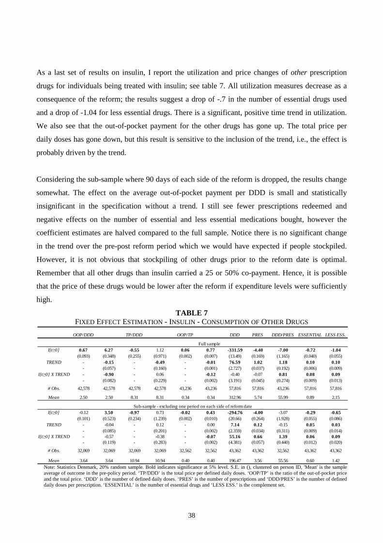
As a last set of results on insulin, I report the utilization and price changes of other prescription
drugs for individuals being treated with insulin; see table 7. All utilization measures decrease as a
consequence of the reform; the results suggest a drop of -.7 in the number of essential drugs used
and a drop of -1.04 for less essential drugs. There is a significant, positive time trend in utilization.
We also see that the out-of-pocket payment for the other drugs has gone up. The total price per
daily doses has gone down, but this result is sensitive to the inclusion of the trend, i.e., the effect is
probably driven by the trend.
Considering the sub-sample where 90 days of each side of the reform is dropped, the results change
somewhat. The effect on the average out-of-pocket payment per DDD is small and statistically
insignificant in the specification without a trend. I still see fewer prescriptions redeemed and
negative effects on the number of essential and less essential medications bought, however the
coefficient estimates are halved compared to the full sample. Notice there is no significant change
in the trend over the pre-post reform period which we would have expected if people stockpiled.
However, it is not obvious that stockpiling of other drugs prior to the reform date is optimal.
Remember that all other drugs than insulin carried a 25 or 50% co-payment. Hence, it is possible
that the price of these drugs would be lower after the reform if expenditure levels were sufficiently
high.
TABLE 7 FIXED EFFECT ESTIMATION - INSULIN - CONSUMPTION OF OTHER DRUGS
Note: Statistics Denmark, 20% random sample. Bold indicates significance at 5% level. S.E. in (), clustered on person ID, 'Mean' is the sample average of outcome in the pre-policy period. ‘TP/DDD’ is the total price per defined daily doses. ‘OOP/TP’ is the ratio of the out-of-pocket price and the total price. ‘DDD’ is the number of defined daily doses. ‘PRES’ is the number of prescriptions and ‘DDD/PRES’ is the number of defined daily doses per prescription. ‘ESSENTIAL’ is the number of essential drugs and ‘LESS ESS.’ is the complement set.
OOP/DDD TP/DDD OOP/TP DDD PRES DDD/PRES ESSENTIAL LESS ESS.
I[t ≥0] 0.67 6.27 -0.55 1.12 0.06 0.77 -331.59 -4.40 -7.00 -0.72 -1.04(0.093) (0.348) (0.255) (0.971) (0.002) (0.007) (13.49) (0.169) (1.165) (0.040) (0.055)
TREND - -0.15 - -0.49 - -0.01 76.59 1.02 1.18 0.10 0.10- (0.057) - (0.160) - (0.001) (2.727) (0.037) (0.192) (0.006) (0.009)
I[t ≥0] X TREND - -0.90 - 0.06 - -0.12 -0.40 -0.07 0.81 0.08 0.09- (0.082) - (0.229) - (0.002) (3.191) (0.045) (0.274) (0.009) (0.013)
# Obs. 42,578 42,578 42,578 42,578 43,236 43,236 57,816 57,816 43,236 57,816 57,816
Mean 2.50 2.50 8.31 8.31 0.34 0.34 312.96 5.74 55.99 0.89 2.15
I[t ≥0] -0.12 3.50 -0.97 0.73 -0.02 0.43 -294.76 -4.00 -3.07 -0.29 -0.65(0.101) (0.523) (0.234) (1.239) (0.002) (0.010) (20.66) (0.264) (1.928) (0.055) (0.086)
TREND - -0.04 - 0.12 - 0.00 7.14 0.12 -0.15 0.05 0.03- (0.085) - (0.201) - (0.002) (2.359) (0.034) (0.311) (0.009) (0.014)
I[t ≥0] X TREND - -0.57 - -0.38 - -0.07 55.16 0.66 1.39 0.06 0.09- (0.119) - (0.283) - (0.002) (4.381) (0.057) (0.440) (0.012) (0.020)
# Obs. 32,069 32,069 32,069 32,069 32,562 32,562 43,362 43,362 32,562 43,362 43,362
Mean 3.64 3.64 10.94 10.94 0.40 0.40 196.47 3.56 55.56 0.60 1.42
Sub-sample - excluding one period on each side of reform date
Full sample
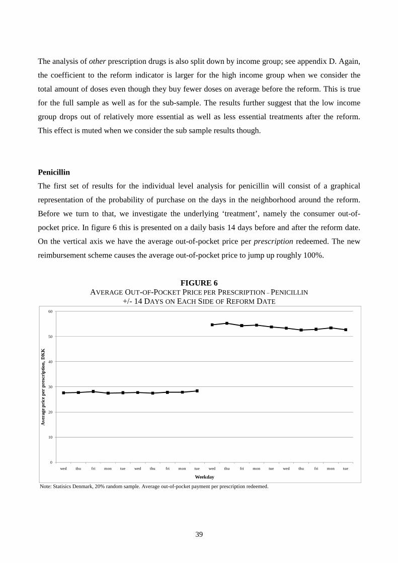
39
The analysis of other prescription drugs is also split down by income group; see appendix D. Again,
the coefficient to the reform indicator is larger for the high income group when we consider the
total amount of doses even though they buy fewer doses on average before the reform. This is true
for the full sample as well as for the sub-sample. The results further suggest that the low income
group drops out of relatively more essential as well as less essential treatments after the reform.
This effect is muted when we consider the sub sample results though.
Penicillin
The first set of results for the individual level analysis for penicillin will consist of a graphical
representation of the probability of purchase on the days in the neighborhood around the reform.
Before we turn to that, we investigate the underlying ‘treatment’, namely the consumer out-of-
pocket price. In figure 6 this is presented on a daily basis 14 days before and after the reform date.
On the vertical axis we have the average out-of-pocket price per prescription redeemed. The new
reimbursement scheme causes the average out-of-pocket price to jump up roughly 100%.
FIGURE 6
AVERAGE OUT-OF-POCKET PRICE PER PRESCRIPTION – PENICILLIN
+/- 14 DAYS ON EACH SIDE OF REFORM DATE
Note: Statisics Denmark, 20% random sample. Average out-of-pocket payment per prescription redeemed.
0
10
20
30
40
50
60
wed thu fri mon tue wed thu fri mon tue wed thu fri mon tue wed thu fri mon tue
Ave
rage
pric
e pe
r pr
escr
iptio
n, D
KK
Weekday

40
Figure 7 presents the empirical propensities to purchase penicillin on a weekly basis before and
after the reform. There are 14 days on each side of the reform date. However the results from
Saturdays and Sundays are not plotted as they contaminate the overall picture (there are very few
purchases on weekends, a graph with the weekends included is placed in Appendix C). The
propensities are marginal effects from a probit estimation with dummies for each individual day,
with the first day (a Wednesday) omitted. That is, the propensities should be seen as deviations
from this day. We see that the propensity to purchase penicillin peaks on Mondays which seems
only natural since GPs are usually closed during the weekends, so people who become sick in the
weekends have to wait till the coming Monday to get a prescription (if they are very sick, they can
go to see at doctor from the emergency service to get a prescription). The purchase propensities on
the remaining weekdays do not seem to be statistically significantly different from each other. More
importantly, an eyeball test shows that there is a downward shift in the propensity to purchase in the
post-reform period.
We now turn to the estimation of the model outlined in equation (1.2) in section 5. Our parameter of
interest, ��, which measures the jump in the propensity caused by the increase in price, will be
estimated using different specifications that controls for the daily variation we observe in figure 7.
Each individual is observed each day in the time period of interest. Estimation is carried out using a
pooled probit9 model with individual level clustering. As a sensitivity check, estimation is
performed using one and two weeks on each side of the reform date, respectively. The results are
reported in table 9.
9 A linear probability model yields almost identical results.

41
FIGURE 7
PURCHASE PROPENSITY – PENICILLIN
+/- 14 DAYS ON EACH SIDE OF REFORM DATE
Note: Statisics Denmark, 20% random sample. Probit estimation of daily purchase propensity around March 1 2000, w. first Wednesday omitted. Dotted line is 95% confidence band.
As we can see in table 9, the coefficient to the reform indicator is negative and highly statistically
significant, suggesting a drop in the propensity to purchase. In order to quantify the drop in the
propensity, I have reported an elasticity measure evaluated at the pre-policy out-of-pocket price.
Using two weeks on each side of the reform date yields price elasticities in the range -.21 to -.30.
The results are not very sensitive to whether we estimate with one or two weeks on each side.
-0.0003
-0.0002
-0.0001
0
0.0001
0.0002
0.0003
thu fri mon tue wed thu fri mon tue wed thu fri mon tue wed thu fri mon tue
Pur
chas
e pr
obab
ility
Weekday
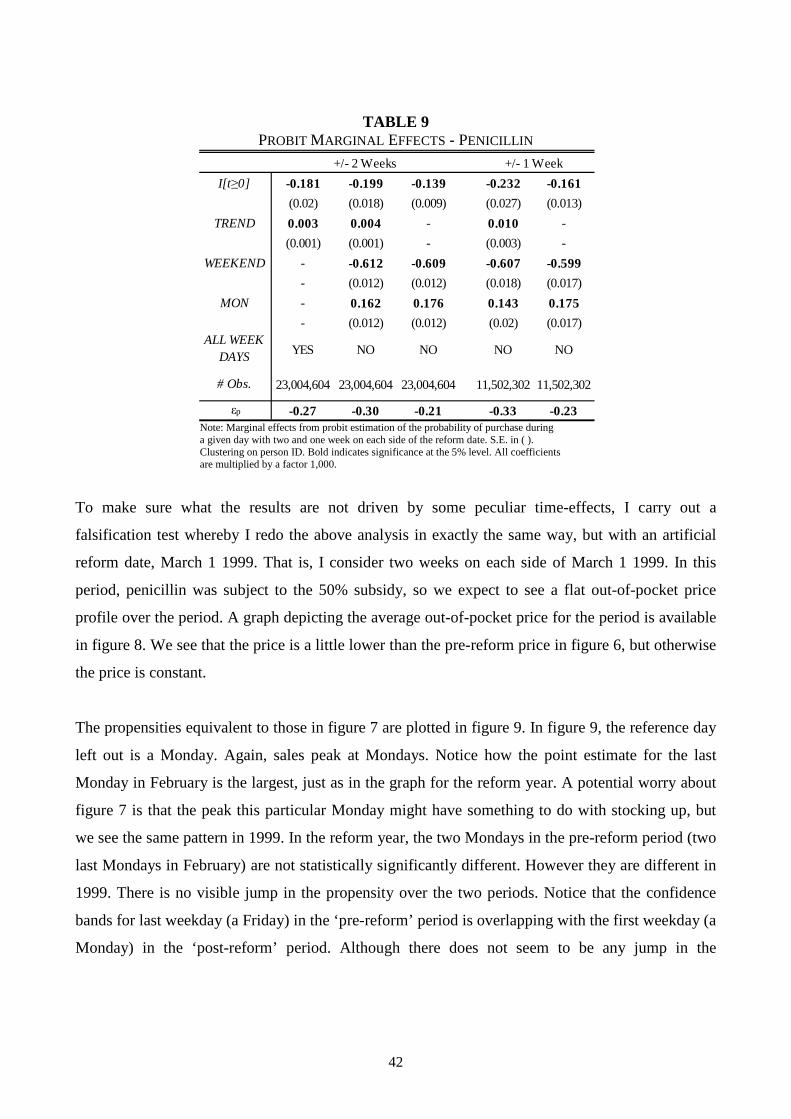
42
TABLE 9 PROBIT MARGINAL EFFECTS - PENICILLIN
Note: Marginal effects from probit estimation of the probability of purchase during a given day with two and one week on each side of the reform date. S.E. in ( ). Clustering on person ID. Bold indicates significance at the 5% level. All coefficients are multiplied by a factor 1,000.
To make sure what the results are not driven by some peculiar time-effects, I carry out a
falsification test whereby I redo the above analysis in exactly the same way, but with an artificial
reform date, March 1 1999. That is, I consider two weeks on each side of March 1 1999. In this
period, penicillin was subject to the 50% subsidy, so we expect to see a flat out-of-pocket price
profile over the period. A graph depicting the average out-of-pocket price for the period is available
in figure 8. We see that the price is a little lower than the pre-reform price in figure 6, but otherwise
the price is constant.
The propensities equivalent to those in figure 7 are plotted in figure 9. In figure 9, the reference day
left out is a Monday. Again, sales peak at Mondays. Notice how the point estimate for the last
Monday in February is the largest, just as in the graph for the reform year. A potential worry about
figure 7 is that the peak this particular Monday might have something to do with stocking up, but
we see the same pattern in 1999. In the reform year, the two Mondays in the pre-reform period (two
last Mondays in February) are not statistically significantly different. However they are different in
1999. There is no visible jump in the propensity over the two periods. Notice that the confidence
bands for last weekday (a Friday) in the ‘pre-reform’ period is overlapping with the first weekday (a
Monday) in the ‘post-reform’ period. Although there does not seem to be any jump in the
I[t ≥0] -0.181 -0.199 -0.139 -0.232 -0.161
(0.02) (0.018) (0.009) (0.027) (0.013)
TREND 0.003 0.004 - 0.010 -
(0.001) (0.001) - (0.003) -
WEEKEND - -0.612 -0.609 -0.607 -0.599
- (0.012) (0.012) (0.018) (0.017)
MON - 0.162 0.176 0.143 0.175
- (0.012) (0.012) (0.02) (0.017)ALL WEEK
DAYS YES NO NO NO NO
# Obs. 23,004,604 23,004,604 23,004,604 11,502,302 11,502,302
εp -0.27 -0.30 -0.21 -0.33 -0.23
+/- 2 Weeks +/- 1 Week

43
propensity, there seems to be a negative trend. The specifications estimated for the reform year are
also performed, and the results at brought in table 10.
FIGURE 8
FALSIFICATION TEST: AVERAGE OUT-OF-POCKET PRICE PER PRESCRIPTION – PENICILLIN
+/- 14 DAYS ON EACH SIDE OF MARCH 1st 1999
Note: Statistics Denmark, 20% random sample. Average out-of-pocket payment per prescription redeemed around March 1 1999. Prices are in 1999 (DKK).
0
10
20
30
40
50
60
mon tue wed thu fri mon tue wed thu fri mon tue wed thu fri mon tuewed thu fri
Ave
rage
pric
e pe
r pr
escr
iptio
n, D
KK
Weekday
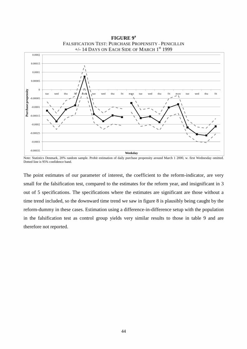
44
FIGURE 9a
FALSIFICATION TEST: PURCHASE PROPENSITY – PENICILLIN
+/- 14 DAYS ON EACH SIDE OF MARCH 1st 1999
Note: Statistics Denmark, 20% random sample. Probit estimation of daily purchase propensity around March 1 2000, w. first Wednesday omitted. Dotted line is 95% confidence band.
The point estimates of our parameter of interest, the coefficient to the reform-indicator, are very
small for the falsification test, compared to the estimates for the reform year, and insignificant in 3
out of 5 specifications. The specifications where the estimates are significant are those without a
time trend included, so the downward time trend we saw in figure 8 is plausibly being caught by the
reform-dummy in these cases. Estimation using a difference-in-difference setup with the population
in the falsification test as control group yields very similar results to those in table 9 and are
therefore not reported.
-0.00035
-0.0003
-0.00025
-0.0002
-0.00015
-0.0001
-0.00005
0
0.00005
0.0001
0.00015
0.0002
tue wed thu fri mon tue wed thu fri mon tue wed thu fri mon tue wed thu fri
Pur
chas
e pr
open
sity
Weekday

45
TABLE 10 PROBIT MARGINAL EFFECTS - FALSIFICATION TEST PENICILLIN
Note: Marginal effects from probit estimation of the probability of purchase during a given day with two and one week on each side of the reform date. S.E. in ( ).Clustering on person ID. Bold indicates significance at the 5% level. All coefficients are multiplied by a factor 1,000.
As a last sensitivity check the individual level analysis on penicillin is split down by income. I
define low/high income as individuals having an income below/above the median income in the
calendar year of 1999. The results shows (in most specifications) that people with low income are
more price responsive than people with high income, see table 10. These findings are consistent
with Simonsen et al. (2010), even though this paper exploits a completely different source of price
variation. It is possible that these findings are related to membership of the private insurance
company “Danmark”: If the probability of membership is positively correlated with income, the
lower price responses by high income consumers may just reflect this. However, the price
elasticities for penicillin reported in this paper are generally in line with the lower estimates in the
literature (see section 2).
To sum up, the analysis shows that the drug reimbursement reform had a positive effect on the
consumer’s out-of-pocket payment and that this was associated with considerable declines in
utilization of both insulin and penicillin. For insulin, the decline in utilization took place on both the
intensive and extensive margin that is, some opted completely out of treatment and those still in
treatment lowered their consumption. The latter is consistent with what is termed ‘drug holidays’ in
the medical literature on non-compliance, i.e., that people stretch a given amount of medication to
cover more days than it has been prescribed for. Alternatively, doctors might have internalized the
cost of the medications that their patients need and adopted a more efficient prescribing pattern. For
I[t ≥0] 0.018 0.009 -0.085 -0.042 -0.033
(0.022) (0.021) (0.01) (0.054) (0.014)
TREND -0.007 -0.007 - 0.001 -
(0.001) (0.001) - (0.008) -
WEEKEND - -0.700 -0.714 -0.746 -0.743
- (0.014) (0.013) (0.027) (0.019)
MON - 0.169 0.189 0.200 0.196
- (0.014) (0.013) (0.028) (0.019)ALL WEEK
DAYS YES NO NO NO NO
# Obs. 22,984,892 22,984,892 22,984,892 11,492,446 11,492,446
+/- 2 Weeks +/- 1 Week

46
penicillin, the analysis suggests a decline on the extensive margin only. The estimated price
responses should be seen as net of private insurance.
TABLE 11 PROBIT MARGINAL EFFECTS - PENICILLIN - BY INCOME
Note: Marginal effects from probit estimation of the probability of purchase during a given day with two and one week on each side of the reform date. S.E. in ( ). Clustering on person ID. Bold indicates significance at the 5% level. All coefficients are multiplied by a factor 1,000. Low/high income is defined as people with income below/above median income.
7. Conclusion
This paper analyzes the effect of increased co-payments on two different prescription drugs, insulin
and penicillin, caused by a reform of the reimbursement scheme for the general public in Denmark.
I show that reliable estimates of the price elasticity of demand can be difficult to uncover if the
source of price variation used is (announced) changes in consumer co-payment. Patients in
treatment with drugs that maintain chronic conditions, such as insulin, are much more likely to
stockpile on their medications if they foresee future price (co-payment) increases. This fact leads us
to overestimate the price response of the consumer. Removing observations close to the date of the
price change reduces this bias, but consumers may have stockpiled to a degree that even this
strategy is not sufficient. Further, the new co-payment system had spillover effects on the
consumption of other essential drugs for people treated with insulin. It is possible that these results
are also driven by stockpiling, even though I argue that stockpiling of other drugs might not be
optimal.
I[t ≥0] -0.210 -0.220 -0.142 -0.235 -0.178 -0.151 -0.178 -0.135 -0.228 -0.144
(0.028) (0.026) (0.013) (0.037) (0.018) (0.028) (0.026) (0.013) (0.038) (0.018)
TREND 0.005 0.005 - 0.008 - 0.001 0.003 - 0.012 -
(0.002) (0.002) - (0.005) - (0.002) (0.002) - (0.005) -
WEEKEND - -0.663 -0.659 -0.659 -0.653 - -0.562 -0.559 -0.555 -0.545
- (0.018) (0.018) (0.026) (0.025) - (0.017) (0.017) (0.024) (0.024)
MON - 0.151 0.169 0.141 0.168 - 0.174 0.184 0.143 0.182
- (0.018) (0.017) (0.027) (0.024) - (0.018) (0.018) (0.028) (0.025)ALL WEEK
DAYS YES NO NO NO NO YES NO NO NO NO
# Obs. 11,474,960 11,474,960 11,474,960 5,737,480 5,737,480 11,529,728 11,529,728 11,529,728 5,764,864 5,764,864
εp -0.30 -0.32 -0.21 -0.32 -0.24 -0.20 -0.24 -0.18 -0.35 -0.22
Low Income High Income
+/- 2 Weeks +/- 1 Week +/- 2 Weeks +/- 1 Week

47
For penicillin, that treats an acute and non-chronic condition, stockpiling is arguably much less
likely. Using a regression discontinuity design in the time dimension, I find the price elasticity of
demand to be in the interval -.18 - -.35. The price response was found to be larger for the lower part
of the income distribution. The size of the estimated price response is comparable to the existing
literature outlined in section 2. That the demand for low income individuals is more price elastic is
consistent with the findings in Simonsen et al. (2010), despite that this paper uses a completely
different source of price variation.
Analyzing the phenomenon of stockpiling more detailed would call for a structural dynamic
approach which also incorporates the non-linear pricing consumers face after the reform. It is
plausible that one would see similar stockpiling patterns under the new subsidy scheme as people
get to the end of their individual subsidy years. This type of behavior points to inherent
inefficiencies of such subsidy schemes. This is, however, not within the scope of this paper and is
left as a point of future research.
Literature Chandra, A., J. Gruber, J. and R. McKnight (2010): “Patient Cost - Sharing and Hospitalization
Offsets in the Elderly”, American Economic Review 100, 193-213.
Contoyannis, P., J. Hurley, P. Grootendorst, S. Jeon and R. Tamblyn (2005): “Estimating the price
elasticity of expenditure for prescription drugs in the presence of non-linear price schedules: an
illustration from Quebec, Canada”, Health Economics 14, 909-923.
Duggan, M., F. Scott Morton: "The Effect of Medicare Part D on Pharmaceutical Prices and
Utilization ", American Economic Review 100, 590-607.
48
Hahn, J., P. Todd, and W. van der Klaauw (2001): “Identification and Estimation of Treatment
Effects with a Regression-Discontinuity Design”, Econometrica 69, 201-209.
Hendel, I., A. Nevo (2006): “Measuring the Implications of Sales and Consumer Inventory
Behavior,” Econometrica, 74(6), 1637- 1673.
Hendel, I., A. Nevo (2009): “A Simple Model of Demand Anticipation”, Mimeo: http://econ-
www.mit.edu/files/4516
Honoré, Bo E. (1992): ”Trimmed LAD and Least Squares Estimation of Truncated and Censored
Regression Models with Fixed Effects”, Econometrica, Vol. 60, 533-565.
Imbens, G. W., and T. Lemieux (2008): “Regression Discontinuity Designs: A Guide to Practise”,
Journal of Econometrics 142, 615-635.
Keeler, E. B., J. P. Newhouse, and C. E. Phelps (1977): “Deductibles and the Demand for Medical
Care Services: the Theory of a Consumer Facing a Variable Price Schedule under Uncertainty”,
Econometrica 45, 641-655.
Lexchin, J., and P. Grootendorst (2004): “Effects of Prescription Drug User Fees on Drugs and
Health Services Use and on Health Status in Vulnerable Populations: A Systematic Review of the
Evidence”, International Journal of Health Services 34, 101-122.
Manning, W. G., J. P. Newhouse, N. Duan, E. B. Keeler, A. Leibowitz, and M. S. Marquis (1987):
Health Insurance and the Demand for Medical Care: Evidence from a Randomized Experiment. The
American Economic Review 77, 251-277.
Newhouse, J. (1993): Free for All: Lessons from the RAND Health Insurance Experiment.
Cambridge, MA. Harvard University Press.
Pavnic, N. (2002): “Do Pharmaceutical Prices Respond to Potential Patient Out-of-Pocket
Expenses?”, RAND Journal of Economics 33, 469-487.

49
Simonsen, M., L. Skipper, and N. Skipper (2010): “Price Sensitivity of Demand for Prescription
Drugs: Exploiting a Regression Kink Design”, Working Paper.
Tamblyn, R., R. Laprise, J. A. Hanley et al. (2001): Adverse Events Associated with Prescription
Drug Cost-Sharing among Poor and Elderly Persons, Journal of the American Medical Association
285, 421-429.

50
Appendix A
Example of an ATC-code. Metformin, used in diabetes treatment.
EXAMPLE OF ATC-CODE
ATC-Code A10BA02
A Alimentary tract and metabolism
(1st level, anatomical main group)
A10 Drugs used in diabetes
(2nd level, therapeutic subgroup)
A10B Oral blood glucose lowering drugs
(3rd level, pharmacological subgroup)
A10BA Biguanides
(4th level, chemical subgroup)
A10BA02 Metformin
(5th level, chemical substance) http://www.whocc.no/atcddd/

51
Appendix B
INSULIN
Total volume of insulin sold per week by ATC-code. Volumes are standardized with means.
The share of the total market of insulin by ATC-code.
Total Volum (DDD) (stand.)
0
1
2
3
4
5
6
7
8
9
10
-52 -32 -12 8 28 48
Week
DD
D
A10AB01
A10AB04
A10AC01
A10AD01
A10AB05
A10AD04
Market Share (DDD)
0
0.1
0.2
0.3
0.4
0.5
0.6
-52 -32 -12 8 28 48
Week
Sh
are
A10AB01
A10AB04
A10AC01
A10AD01
A10AB05
A10AD04

52
The average total price of insulin per DDD by ATC-code.
The total number of insulin prescriptions redeemed per week.
Note: Statistics Denmark. 20% random sample. Number of filed prescriptions per day, insulin.
Avg. Total Price per DDD (in DKK)
0
2
4
6
8
10
12
14
16
-52 -32 -12 8 28 48
Week
DK
K p
er
DD
D
A10AB01
A10AB04
A10AC01
A10AD01
A10AB05
A10AD04
0
1
2
3
4
5
6
7
-52 -32 -12 8 28 48
Pre
scrip
tions
Week
Number of Prescriptions per Week(1,000)
Series1

53
The total number of people buying insulin per week.
Note: Statistics Denmark. 20% random sample. Number of persons receiving treatment per day, insulin.
0
0.5
1
1.5
2
2.5
3
3.5
4
-52 -32 -12 8 28 48
Per
sons
Week
Persons per Week (1,000)

54
PENICILLIN
Total number of penicillin prescriptions redeemed.
Note: Statistics Denmark. 20% random sample. Number of prescriptions filed per day, penicillin.
Total number of people buying penicillin.
Note: Statistics Denmark. 20% random sample. Number of persons receiving treatment per day, penicillin.
0
1
2
3
4
5
6
7
-52 -32 -12 8 28 48
Pre
scrip
tions
Week
Number of Prescriptions per Week (1,000)
0
0.5
1
1.5
2
2.5
3
3.5
4
4.5
5
-52 -32 -12 8 28 48
Per
sons
Week
Persons per Week (1,000)

55
Appendix C Relative probabilities to purchase penicillin around March 1 1999 with 14 days on each side of that date.
Note: Statistics Denmark, 20% random sample. Probit estimation of daily purchase propensity around March 1 2000, w. first Wednesday omitted. Dotted line is 95% confidence band.
-0.0006
-0.0005
-0.0004
-0.0003
-0.0002
-0.0001
0
0.0001
0.0002
0.0003
0.0004
thu fri sat sun mon tue wed thu fri sat sun mon tue wed thu fri sat sun mon tue wed thu fri sat sun mon tue
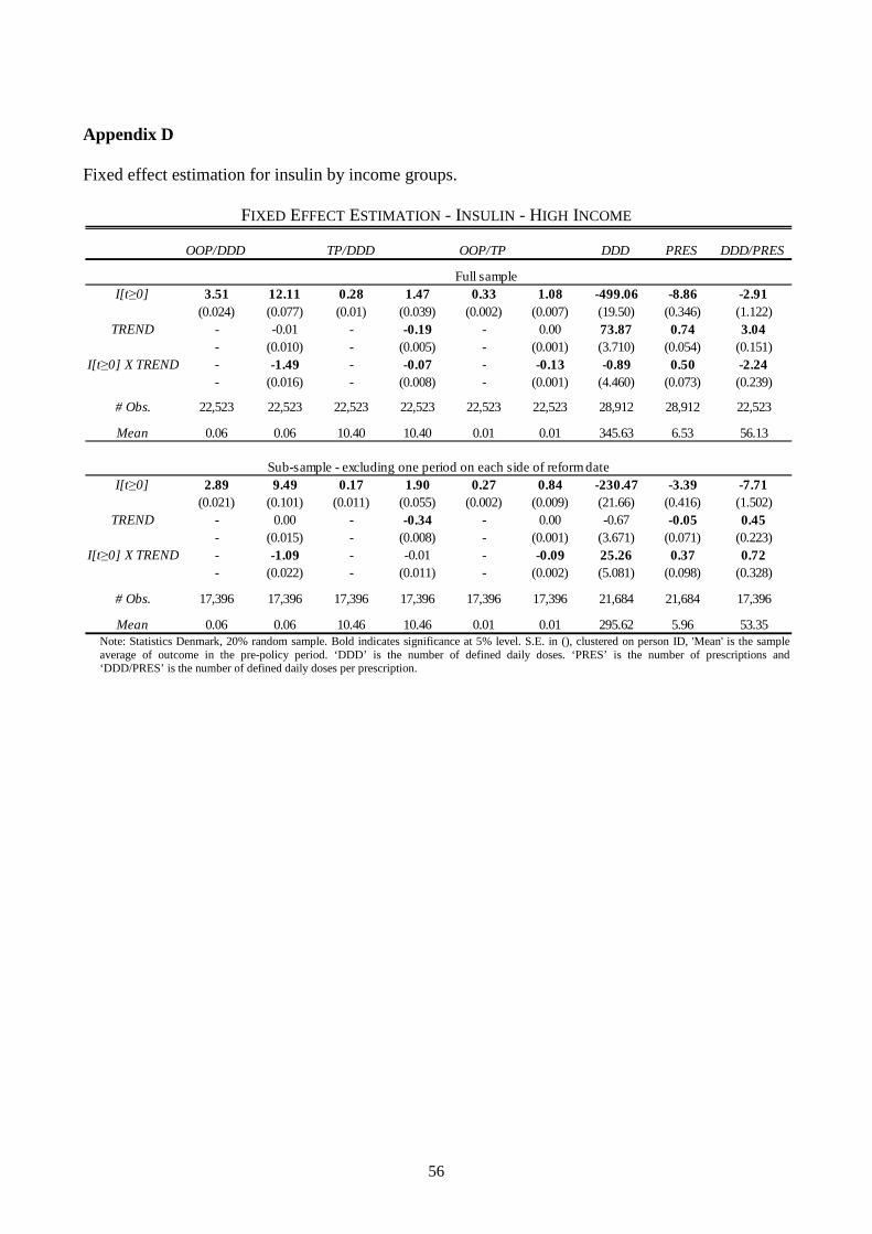
56
Appendix D Fixed effect estimation for insulin by income groups.
FIXED EFFECT ESTIMATION - INSULIN - HIGH INCOME
Note: Statistics Denmark, 20% random sample. Bold indicates significance at 5% level. S.E. in (), clustered on person ID, 'Mean' is the sample average of outcome in the pre-policy period. ‘DDD’ is the number of defined daily doses. ‘PRES’ is the number of prescriptions and ‘DDD/PRES’ is the number of defined daily doses per prescription.
OOP/DDD TP/DDD OOP/TP DDD PRES DDD/PRES
I[t ≥0] 3.51 12.11 0.28 1.47 0.33 1.08 -499.06 -8.86 -2.91(0.024) (0.077) (0.01) (0.039) (0.002) (0.007) (19.50) (0.346) (1.122)
TREND - -0.01 - -0.19 - 0.00 73.87 0.74 3.04- (0.010) - (0.005) - (0.001) (3.710) (0.054) (0.151)
I[t ≥0] X TREND - -1.49 - -0.07 - -0.13 -0.89 0.50 -2.24- (0.016) - (0.008) - (0.001) (4.460) (0.073) (0.239)
# Obs. 22,523 22,523 22,523 22,523 22,523 22,523 28,912 28,912 22,523
Mean 0.06 0.06 10.40 10.40 0.01 0.01 345.63 6.53 56.13
I[t ≥0] 2.89 9.49 0.17 1.90 0.27 0.84 -230.47 -3.39 -7.71(0.021) (0.101) (0.011) (0.055) (0.002) (0.009) (21.66) (0.416) (1.502)
TREND - 0.00 - -0.34 - 0.00 -0.67 -0.05 0.45- (0.015) - (0.008) - (0.001) (3.671) (0.071) (0.223)
I[t ≥0] X TREND - -1.09 - -0.01 - -0.09 25.26 0.37 0.72- (0.022) - (0.011) - (0.002) (5.081) (0.098) (0.328)
# Obs. 17,396 17,396 17,396 17,396 17,396 17,396 21,684 21,684 17,396
Mean 0.06 0.06 10.46 10.46 0.01 0.01 295.62 5.96 53.35
Full sample
Sub-sample - excluding one period on each side of reform date

57
FIXED EFFECT ESTIMATION - INSULIN - LOW INCOME
Note: Statistics Denmark, 20% random sample. Bold indicates significance at 5% level. S.E. in (), clustered on person ID, 'Mean' is the sample average of outcome in the pre-policy period. ‘DDD’ is the number of defined daily doses. ‘PRES’ is the number of prescriptions and ‘DDD/PRES’ is the number of defined daily doses per prescription.
Fixed effect estimation of consumption of other drugs by income groups.
FIXED EFFECT ESTIMATION - INSULIN - CONSUMPTION OF OTHER DRUGS - HIGH INCOME
Note: Statistics Denmark, 20% random sample. Bold indicates significance at 5% level. S.E. in (), clustered on person ID, 'Mean' is the sample average of outcome in the pre-policy period. ‘DDD’ is the number of defined daily doses. ‘PRES’ is the number of prescriptions and ‘DDD/PRES’ is the number of defined daily doses per prescription. ‘ESSENTIAL’ is the number of essential drugs and ‘LESS ESS.’ is the complement set.
OOP/DDD TP/DDD OOP/TP DDD PRES DDD/PRES
I[t ≥0] 2.85 9.41 0.33 1.42 0.27 0.85 -400.61 -7.15 -3.93(0.02) (0.064) (0.009) (0.033) (0.002) (0.006) (17.62) (0.331) (1.006)
TREND - -0.02 - -0.23 - -0.001 74.08 0.76 2.99- (0.009) - (0.005) - (0.001) (3.564) (0.055) (0.146)
I[t ≥0] X TREND - -1.14 - -0.02 - -0.101 -13.13 0.26 -2.02- (0.014) - (0.007) (0.001) (4.247) (0.074) (0.221)-
# Obs. 22,748 22,748 22,748 22,748 22,748 22,748 28,912 28,912 22,748
Mean 0.06 0.06 10.26 10.26 0.01 0.01 394.06 7.52 54.85
I[t ≥0] 2.3 6.99 0.19 1.89 0.22 0.62 -165.64 -1.77 -9.07(0.017) (0.081) (0.011) (0.049) (0.002) (0.008) (22.48) (0.454) (1.368)
TREND - 0.00 - -0.38 - 0.00 8.32 0.14 0.49- (0.012) - (0.007) - (0.001) (3.947) (0.078) (0.211)
I[t ≥0] X TREND - -0.77 - 0.04 - -0.07 9.35 -0.02 0.97- (0.018) - (0.011) - (0.002) (5.309) (0.107) (0.304)
# Obs. 17,400 17,400 17,400 17,400 17,400 17,400 21,684 21,684 17,400
Mean 0.07 0.07 10.34 10.34 0.01 0.01 345.29 6.99 52.28
Full sample
Sub-sample - excluding one period on each side of reform date
OOP/DDD TP/DDD OOP/TP DDD PRES DDD/PRES ESSENTIAL LESS ESS.
I[t ≥0] 1.11 9.26 -0.61 2.56 0.08 0.91 -356.61 -4.48 -10.66 -0.66 -0.84(0.187) (0.704) (0.521) (1.967) (0.004) (0.011) (21.82) (0.243) (2.024) (0.060) (0.076)
TREND - -0.25 - -0.91 - -0.01 85.96 1.07 1.34 0.09 0.09- (0.115) - (0.321) - (0.002) (4.596) (0.056) (0.331) (0.008) (0.013)
I[t ≥0] X TREND - -1.28 - 0.09 -0.14 -2.72 -0.09 1.26 0.08 0.07- (0.165) - (0.460) (0.002) (5.236) (0.067) (0.474) (0.013) (0.018)
# Obs. 18,851 18,851 18,851 18,851 19,279 19,277 28,912 28,912 19,279 28,912 28,912
Mean 3.39 3.39 10.19 10.19 0.39 0.39 233.15 4.09 56.83 0.63 1.46
I[t ≥0] -0.05 5.86 -1.38 2.10 -0.02 0.57 -360.18 -4.65 -5.21 -0.29 -0.66(0.185) (1.081) (0.434) (2.304) (0.003) (0.016) (33.40) (0.390) (3.409) (0.080) (0.122)
TREND - -0.06 - 0.24 - 0.00 9.24 0.16 -0.28 0.03 0.02- (0.175) - (0.373) - (0.002) (3.591) (0.052) (0.550) (0.013) (0.019)
I[t ≥0] X TREND - -0.93 - -0.78 - -0.09 65.38 0.75 1.85 0.08 0.10- (0.247) - (0.526) - (0.003) (7.075) (0.085) (0.777) (0.018) (0.028)
# Obs. 14,201 14,201 14,201 14,201 14,522 14,522 21,684 21,684 14,522 21,684 21,684
Mean 2.63 2.63 8.66 8.66 0.34 0.34 273.39 5.16 54.91 0.85 2.10
Sub-sample - excluding one period on each side of reform date
Full sample

58
FIXED EFFECT ESTIMATION - INSULIN - CONSUMPTION OF OTHER DRUGS - LOW INCOME
Note: Statistics Denmark, 20% random sample. Bold indicates significance at 5% level. S.E. in (), clustered on person ID, 'Mean' is the sample average of outcome in the pre-policy period. ‘DDD’ is the number of defined daily doses. ‘PRES’ is the number of prescriptions and ‘DDD/PRES’ is the number of defined daily doses per prescription. ‘ESSENTIAL’ is the number of essential drugs and ‘LESS ESS.’ is the complement set.
OOP/DDD TP/DDD OOP/TP DDD PRES DDD/PRESESSENTIALLESS ESS.
I[t ≥0] 0.33 4.04 -0.51 0.044 0.05 0.67 -315.81 -4.34 -4.23 -0.75 -1.19(0.079) (0.296) (0.219) (0.832) (0.003) (0.008) (17.11) (0.233) (1.350) (0.052) (0.078)
TREND - -0.07 - -0.17 - -0.002 70.33 0.98 1.05 0.10 0.10- (0.049) - (0.138) - (0.001) (3.373) (0.046) (0.224) (0.007) (0.012)
I[t ≥0] X TREND - -0.62 - 0.02 - -0.110 1.32 -0.07 0.47 0.08 0.11- (0.070) - (0.196) - (0.002) (4.003) (0.058) (0.319) (0.011) (0.018)
# Obs. 23,729 23,729 23,729 23,729 23,959 23,959 28,912 28,912 23,959 28,912 28,912
Mean 1.79 1.79 6.81 6.81 0.30 0.30 392.74 7.39 55.31 1.15 2.85
I[t ≥0] -0.16 1.70 -0.66 -0.33 -0.03 0.32 -248.65 -3.50 -1.41 -0.28 -0.63(0.075) (0.412) (0.245) (1.299) (0.003) (0.012) (26.23) (0.356) (2.178) (0.074) (0.120)
TREND - -0.03 - 0.03 - -0.001 5.59 0.09 -0.06 0.06 0.03- (0.066) - (0.210) - (0.002) (3.149) (0.044) (0.351) (0.011) (0.018)
I[t ≥0] X TREND - -0.29 - -0.08 - -0.06 48.07 0.59 1.02 0.05 0.09- (0.094) - (0.297) - (0.003) (5.570) (0.076) (0.497) (0.016) (0.027)
# Obs. 17,869 17,869 17,869 17,869 18,041 18,041 21,684 21,684 18,041 21,684 21,684
Mean 1.83 1.83 6.86 6.86 0.30 0.30 350.29 6.75 54.40 1.11 2.79
Full sample
Sub-sample - excluding one period on each side of reform date

59
CHAPTER 2
Price Sensitivity of Demand for Prescription Drugs:
Exploiting a Regression Kink Design

60

61
Price Sensitivity of Demand for Prescription Drugs:
Exploiting a Regression Kink Design
Marianne Simonsen
School of Economics
and Management
Aarhus University
Lars Skipper
Aarhus School of
Business
Aarhus University
Niels Skipper
School of Economics
and Management
Aarhus University
November, 2010
Abstract:
This paper investigates price sensitivity of demand for prescription drugs, using drug purchase
records for a 20 % random sample of the Danish population. We identify price responsiveness by
exploiting exogenous variation in prices caused by kinked reimbursement schemes and implement a
regression kink design. Thus, within a unifying framework we uncover price sensitivity for different
subpopulations and types of drugs. The results suggest low average price responsiveness with
corresponding price elasticities ranging from -0.09 to -0.25, implying that demand is inelastic.
However, individuals with lower education and income are more responsive to the price. Also,
essential drugs that prevent deterioration in health and prolong life have lower associated average
price sensitivity.
Key words: Prescription drugs, price, reimbursement schemes, regression kink design
JEL codes: I11, I18
Acknowledgements: We greatly appreciate valuable comments from Søren Leth-Petersen, Emilia
Simeonova, Michael Svarer, and Torben Sørensen. The paper has benefited from comments
received at the 2007 iHEA conference, the 1st meeting of the Danish Microeconometric Network
2009, and at seminars at the Stockholm School of Economics, the Swedish Institute for Social
Research, University of Stockholm, IZA, Bonn and Carlos III, Madrid. The usual disclaimer
applies.

62
1. Introduction
During 1998-2007, real pharmaceutical spending within the OECD went up almost 50 %, reaching
more than USD 650 billion in 2007. Furthermore, drug spending (prescription and non-prescription)
amounted to an impressive 15 % of total health spending with a US growth that was more than
twice that of total health expenditures; see OECD (2009). Spending on pharmaceuticals is foreseen
to increase even further in the future, putting severe pressure on health care budgets. To control
such spending, there is increased interest in designing optimal health insurance schemes. Necessary
inputs into the construction of health insurance policies are reliable estimates of price sensitivity of
demand, yet the empirical evidence in this area is limited, and the existing estimates vary
considerably. Furthermore, different subgroups in the population do not invest the same in their
own health and do not face the same budget constraints. To the extent that subgroups will also react
differently to prices of prescription drugs, subgroup specific estimates are crucial.
Clearly, the task of uncovering price sensitivity of demand for drugs is complicated by the standard
selection problem: individuals who purchase prescription drugs do not constitute a random part of
the population; presumably they have a higher willingness to pay than individuals who refrain from
buying. Moreover, conditional on purchasing, the price people face is non-random. Even if studies
attempt to deal with these essential identification problems, they are often not able to distinguish
spending on one type of prescription drug from other types, or even from different types of health
care usage such as hospital admittance. In other cases, the type of drug is known, but the price is
not. This is typically solved by a combination of substantial assumptions and an imputation
strategy. Finally, identification strategies often restrict the results to hold only for a specific
subgroup of the overall population.
The perhaps most widely known study within this field is the RAND Health Insurance Experiment
(HIE), which ran from the late 1970’s to the start of the 1980’s. The unique feature of the HIE was
that insurance plans for non-aged individuals (61 or below) were randomly assigned in six different
locations across the US. The insurance plans differed in the size of the deductible amount, co-
insurance rates and full stop-loss; an annual limit on out-of-pocket expenditures. In this sense, the
study had the flavor of a randomized experiment, which has led many to consider it the gold
standard in the literature. In the study, the average price elasticity of overall health care demand,

63
including prescription drugs, hospital utilization and other health care services, was estimated to be
-0.20, see Manning et al. (1987) and Newhouse (1993).
While well executed and evaluated, an important limitation of the RAND HIE was that it did not
consider the elderly population, which accounts for a large share of medical expenditures.
Recognizing this point, Contoyannis et al. (2005) estimate the price elasticity for prescription drugs
in the presence of a nonlinear price schedule for the elderly people (age 65 or over) enrolled in the
Quebec Public Pharmacare program in Canada, exploiting time variation in cost-sharing. Their
overall finding is a price elasticity ranging from -0.12 to -0.16. Similarly, Chandra et al. (2010)
study price responsiveness for people enrolled in California Public Employees Retirement System
(CalPERS) with focus on the elderly population. In 2001 co-payments went up for the fraction of
enrollees under Preferred Provider Organizations (PPO), and in 2002 co-payments were increased
for the fraction that received care through HMO’s. Applying a difference-in-difference framework,
the authors estimate drug utilization elasticities with respect to patient cost. Resulting elasticities are
in line with the RAND HIE.
Acknowledging the fact that price elasticities for prescription drugs are likely to be just as
heterogeneous across types of drugs as price elasticities for other types of products, Goldman et al.
(2004) and Landsman et al. (2005) study price responsiveness for different types of therapeutic
groups. Using regression type analyses on pharmacy claims data combined with cross-sectional
variation in health plan benefits designs, both studies find that drugs used for chronic conditions are
less price sensitive (-0.1 to -0.2) than drugs used for more acute conditions (-0.3 to -0.6).
Furthermore, Tamblyn et al. (2001) consider both the elderly population and welfare participants in
Quebec, Canada and find that demand for essential drugs reacts less to the introduction of
prescription drug cost-sharing than demand for less essential drugs.
In this paper, we add to the scarce but growing literature and investigate the issue of whether
demand for prescription drugs is sensitive to the price. We estimate the change in the propensity to
consume caused by a change in the price. All estimates of price sensitivity are uncovered within a
context where individuals may be forward-looking and within a market where private health
insurance – that may cover part of or all costs related to prescription drugs – exists. We believe that
these are the policy relevant parameters if one is interested in changing the current system

64
marginally.1 We use a rich register-based data set on a 20 % random sample of the Danish
population in the period 2000-2003. Contrary to many existing data sets, ours includes information
on therapeutic group, price, and out-of-pocket payment for every prescription drug purchase. These
data are augmented with socio-economic characteristics on a yearly basis. Besides superior data,
our main contributions are the following: 1) we use a regression kink design to overcome the
standard selection problem. The idea is very close to that of a regression discontinuity design (see
for example Lee and Lemieux (2009)) except that instead of a shift in levels, we exploit a shift in
slopes.2 Here we directly exploit that coinsurance payments decrease in a discontinuous fashion as
consumption (on a yearly basis) increases. In principle, there is no reason to think that individuals
just above a given kink point are different from individuals just below – except for the fact that the
price faced by individuals below the kink point decreases less with total consumption than for
individuals above the kink point. Comparing the propensity to purchase for individuals who are just
above with that for individuals who are just below kink points then allows us to identify price
sensitivities. While we are not the first to acknowledge the existence of this type of identification,
see for example Guryan (2003) and Nielsen, Taber and Sørensen (2010), we are, to the best of our
knowledge, among the very first to directly implement such a design. Recently, Card, Lee and Pei
(2009) have established conditions under which the regression kink design nonparametrically
identifies the “local average response” (Altonji and Matzkin (2005)) or, equivalently, the “treatment
on the treated” (Florens, Heckman, Meghir and Vytlacil (2008)). Card, Lee and Pei (2009) and
Nielsen, Taber and Sørensen (2010) provide the only other direct implementation of a regression
kink design that we are aware of. 2) Health insurance is universally supplied by the Danish
government. This enables us to use a unifying identification strategy to consider estimates for the
entire Danish population as well as estimates for subgroups defined by socio-economic
characteristics. Using the same identification strategy for all subgroups makes it much easier to
compare estimates across subgroups. This is a major advantage compared to the existing studies
that either only have access to (or exploit) a relatively young (RAND HIE) or old (Contoyannis et
al. (2005), Chandra et al. (2010)) population or do not distinguish between subpopulations. We
demonstrate that estimates for relevant subgroups are of reasonable size and relate to each other in a
1 Of course, our estimates are uninformative about underlying price sensitivity in the absence of a private health insurance market. 2 In particular the tax literature has devoted considerable attention to kinks (in budget sets); see Moffitt (1990) for an early overview. Recently, these kinks have also been used as the basis for identification, for example to investigate the responsiveness of labor supply to tax schemes; see Saez (2009) and Chetty et al. (2009). In fact, various non-linear pricing schedules are often exploited to generate instruments in the economics literature; for recent examples see Rothstein and Rouse (2007), Nielsen, Sørensen and Taber (2008), and Dynarski, Gruber and Li (2009).

65
meaningful way, which clearly increases the credibility of the overall identification strategy. 3)
Finally, in addition to providing subpopulation specific estimates, we also distinguish between
types of drugs, something which is rarely possible simply because of lack of data.
Our results suggest that demand is inelastic; we find low average price responsiveness with a
corresponding price elasticity ranging from -0.09 to -0.25, thus comparable to the results from the
RAND HIE for the overall population. Individuals with lower education and income are, however,
more responsive to the price. The same is true for the elderly population, and our estimates are in
line with those of Chandra et al. (2010) and Contoyannis et al. (2005). Finally, essential drugs that
surely prevent deterioration of health and prolong life have, as expected, much lower associated
average price sensitivity than the complementary set of drugs.
The remaining part of the paper is organized as follows: Section 2 presents details of the Danish
market for outpatient prescription drugs and subsidy policies. Section 3 presents the conceptual
framework including a stylized economic model of drug purchase and links the model to parameters
of interest and identification strategy. Section 4 outlines the features of the available data. Section 5
gives the results from the empirical analysis, and Section 6 concludes.
2. The Danish Market for Outpatient Prescription Drugs
The Danish market for outpatient prescription drugs is highly regulated to secure correct handling
of as well as uniform prices on drugs across pharmacies. Pharmaceutical companies report
pharmacy purchase prices to the Danish Medicines Agency, who then announces retail prices.
These retail prices (along with a comprehensive list of information about the specific drugs
including substitutable drugs3) are made publicly available and registered online for five years.
Furthermore, changes in purchase prices must be reported by the pharmaceutical companies two
weeks in advance. Pharmacies must sell the cheapest substitute to prescription drugs unless the
prescribing doctor requires otherwise, or the patient specifically asks for another synonymous drug.4
Doctors do not have monetary incentives to prescribe more or less expensive drugs.
3 Substitutes are defined by having the same dose of the active substance as well as the same use (tablets, capsules etc). 4 Before 1997, the physician was required to write on the prescription if substitution was allowed.

66
Just as in the rest of OECD, consumption of prescription drugs has increased in a Danish context.
Figure 1 shows average level of consumption in Danish Crowns (DKK)5 in the period from 1995 –
2003 (in 1995 prices). On average, a Dane spent roughly DKK 1,750 on prescription drugs in 2003,
while the median was around DKK 400. In comparison, the average patient in treatment for
diabetes spent about DKK 4,400 on insulin and analogous products alone, the average patient in
treatment for excess gastric acid production spent about DKK 1,300 on relevant products, while
individuals in treatment with penicillin spent on average DKK 158.6
FIGURE 1
AVERAGE CONSUMPTION OF PRESCRIPTION DRUGS OVER TIME (DKK IN 1995)
The subsidy scheme for adults 2000 - 2003
Subsidies were (and still are) based on the price of the products. Until June 25 2001, subsidies were
based on the average price of the two cheapest substitutes. This was designated the reference price. 5 € 100 corresponds to DKK 745 as of March 18 2009. 6 Insulin and analogous products identified by ATC code A10A, treatments for excess gastric acid production ATC code A02A, penicillin ATC code J01C. See the Danish Medicines Agency for aggregate statistics, www.medicinpriser.dk and p. 20 for a description of the ATC system.
1,200
1,300
1,400
1,500
1,600
1,700
1,800
1,900
1995 1996 1997 1998 1999 2000 2001 2002 2003

67
After June 25 2001, this was replaced by a system where subsidies were based on the cheapest
product among substitutes. This was called the subsidy price. However, if one or more of the
substitutable products were sold within EU, the subsidy price would not be based on the Danish
price but on the average price within EU.7 Finally, products subject to parallel import received the
same subsidy as the original product sold in Denmark.
Starting in March 2000, individual level purchases of subsidized products (see section below for a
description) were entered into a central register, from which all pharmacies get their information,
and total costs were accumulated from the time of first purchase.8 Accumulated total costs (from
now on TC) are measured in reference/subsidy prices. Current TC is printed on receipts from drug
purchases and thus always available to a potential customer. Furthermore, the Danish Medicines
Agency provides a web page, www.medicinpriser.dk, where individuals can enter relevant
information and check the price they face for a potential product before going to the pharmacy. A
call to the pharmacy will yield the same information for those not connected to the internet.
TABLE 1
THE SUBSIDY SCHEME 2000 – 2003
Table 1 describes the subsidy scheme. If an individual has a TC below a given threshold prior to
purchasing and the price of buying a product brings TC above the threshold, the consumer will
receive the lower subsidy for the part of the price below the threshold and the higher subsidy for the
part of the price above the threshold. To give an example, consider an individual who considers
buying a product worth DKK 100. Assume that she has a TC of DKK 400 prior to the purchasing
decision. In this case, she is not subject to any subsidy should she decide to buy, and she will face
7 Prices in Greece, Spain, Portugal, and Luxemburg were excluded because income levels in these countries differed substantially from that of Denmark. 8 Before March 2000, co-insurance rates were fixed at either 50 or 75 % depending on the type of product. An exception was Insulin to treat diabetes, which was free of costs. See Skipper (2009) for an analysis of the introduction of the new subsidy scheme.
Mar.-Dec. 2000 2001 2002 2003DKK DKK DKK DKK
0 % of TC 0 - 500 0 - 510 0 - 515 0 - 54050 % of TC 500 - 1,200 510 - 1,230 515 - 1,240 540 - 1,30075 % of TC 1,200 - 2,800 1,230 - 2,875 1,240 - 2,900 1,300 - 3,04085 % of TC 2,800 + 2,875 + 2,900 + 3,040 +

68
the full price of DKK 100. Assume then instead that her TC prior to purchasing is DKK 450. Now
she will receive no subsidy for DKK 50 and a 50 % subsidy for the DKK 50 that brings her TC
account above the threshold point. In this alternative scenario, the price faced by the individual is
DKK 75.
A year after the first purchase of prescription drugs, TC is re-zeroed. The structure of the subsidies
forms the basis for identifying the effect of prices on demand for prescription drugs as described in
the following section.
Retail prices of most prescription drugs are subsidized by the government, leading to a general
subsidy, though some are only subsidized if the individual has a specific diagnosis or is officially
retired. This is called a conditional subsidy.
Apart from general and conditional subsidies, an individual can receive one-product, increased,
chronic’s, terminal , and municipality specific subsidies. In our data, we can identify the type of
subsidy individuals receive. One-product subsidies concern a specific type of product (and all its
substitutes) that is subject to neither a general nor a conditional subsidy. A general practitioner
makes the application on behalf of the patient, and the Danish Medicines Agency is the decision-
making authority. If the subsidy is granted, all purchases of the given product will be added to TC
in the same manner as purchases of products with general or conditional subsidies. Typically, the
subsidy will be granted for life but may in certain cases be shorter (for example if the product is not
to be consumed over an extended period).
As pointed out above, general and conditional subsidies are based on the subsidy price. In very rare
cases, individuals are granted an increased subsidy based on a more expensive product. This only
occurs if the patient is allergic to a cheaper alternative or suffers from serious side-effects. The
application procedure is the same as for one-product subsidies, and, if granted, purchases are added
to TC. Again, the subsidy is typically granted for life.
Chronically ill individuals with a predicted yearly TC above a certain threshold (around DKK
18,000 in the 2000-2003 period) may receive full compensation for any purchases above this value.
The application procedure is the same as above, but subsidies are only for a five-year period. In

69
2001 and 2002, 9,084 and 8,141 people out of a population of about 5.5 million people received
chronic’s subsidies. Terminally ill patients who choose to spend the remaining time of their life at
home instead of being hospitalized do not pay for any drug purchases (inpatient prescription drug
consumption is free of charge as well). In 2001, 8,430 people received terminal subsidies, and in
2002 the number was 8,568. Finally, municipalities may choose to provide further subsidies. These
are typically granted to low-wealth, low-income retirees.
As in most countries, there exists a private health insurance market as well. The most important
player in the market for prescription drugs is the company, ”Danmark”. “Danmark” insures about 2
million Danes. Crucial for our study is that none of the policies of “Danmark” change at the kink
points described above. In fact, none of “Danmark’s” policies change with yearly consumption of
prescription drugs. Furthermore, it is not possible to enroll if one has purchased any prescription
drugs during the last 12 months.9 The company offers four types of policies; Group 1, 2, 5, and
Basis. Groups 1 and 2 insurance (about 400,000 individuals in total) cover all prescription drug
expenditures related to products granted one of the government subsidies described above and 50 %
of all costs related to products without any government subsidy. Group 5 insurance (1.3 million
individuals) covers 50 % of expenditures towards products receiving any government subsidy and
25 % of costs related to products without any subsidy. Basis insurance does not cover any costs of
drug purchase, but individuals buying this type of insurance may – no matter their health status –
opt into any of the other insurance policies at any point in time. Group 1 insurance has a yearly cost
of about DKK 2,400 (in 2007), Group 2 insurance costs DKK 3,200, Group 5 insurance about DKK
1,000, and Basis about DKK 400. When we discuss our identification strategy below, we will also
explicitly address the implications of this private option.10
3. Conceptual Framework
In order to emphasize the identifying assumptions behind our estimation strategy and to provide a
framework for interpreting our empirical results, this section firstly presents a stylized economic
model of drug purchase. The model is set within the regime described in Section 2 above, where the
9 Individuals aged 61 or above cannot enrol either. 10 We are in the process of gathering survey information about membership of “Danmark” (SUSY survey 2000, available from the Danish Data Archive). With this secondary data set in hand, we can model membership and then subsequently predict membership in our register data. This should allow us to investigate the sensitivity of our results for groups with and without private insurance.

70
crucial feature is that prescription drug subsidies vary with total consumption. We next discuss
parameters of interest and identification.
At each point in time, an individual experiences a risk of becoming ill and an associated need to buy
a given prescription drug. This risk is specific to the individual and may vary with characteristics,
observable as well as unobservable, and behavior. Therefore, at each point in time, the individual
must decide whether or not to purchase the drug. Since prescription drug purchase, by definition,
requires a prescription from a general practitioner, only individuals who experience medically
substantiated needs are able to do so. Individuals can decide to buy the drug in the amount
prescribed by the general practitioner or not; he cannot decide on a different amount or an entirely
different product. Because drug purchase is costly to the individual both in terms of foregone
consumption and time, not all individuals may choose to buy the drug, although it is expected to
alleviate pain and/or cure the disease (primary noncompliance), or individuals may take smaller
amounts than what is prescribed (secondary noncompliance), for example by taking what is known
as ‘drug-holidays’.
Consider a simple two-period model, � � 1,2. Assume for simplicity that there is only one kink in
the subsidy scheme outlined above and that both � � 1,2 lie within the same subsidy year (i.e.
before TC is re-zeroed). Other kinks can easily be incorporated. Assume that we are initially in a
neighborhood around the kink point. As hinted at above, this is the region that provides us with
identifying variation. If we are on the right hand side of the kink point, purchases in � � 1 will not
affect the price of potential purchases in � � 2. If we are on the left hand side, however, this is no
longer true. Formally let:
� � � � �� � � ,
where the price without any subsidy is denoted � , and �� is measured prior to the purchasing
decision.
Assume that utility is additively separable across time. Consider now the net value of purchasing
relative to not in period 1:
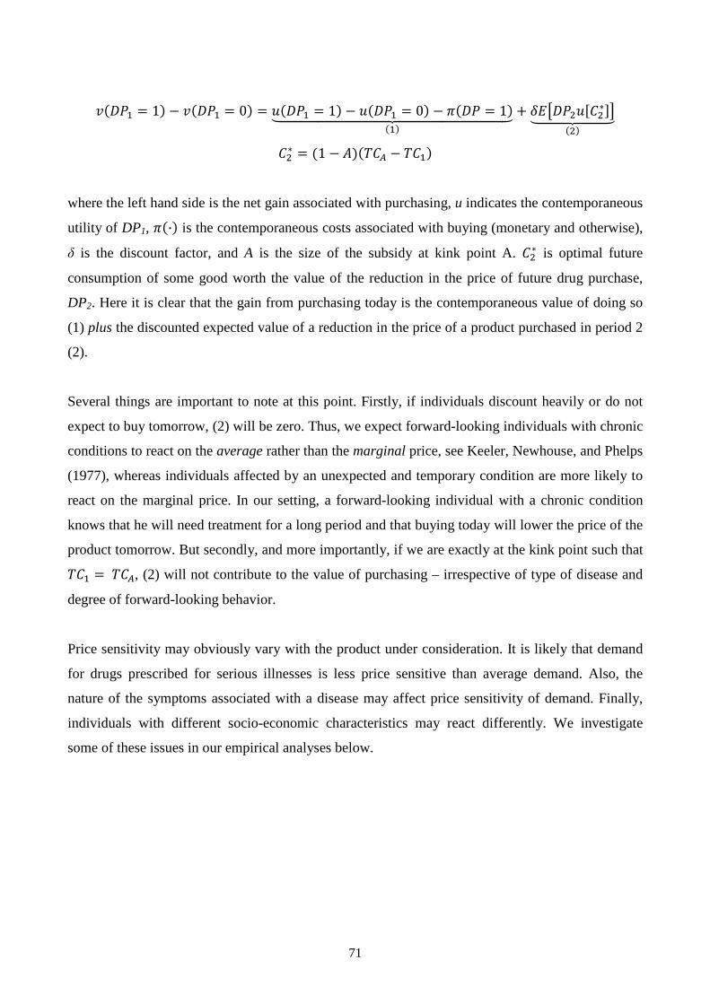
71
����� � 1� � ����� � 0� � ����� � 1� � ����� � 0� � ���� � 1������������������������������� � ������� �!"#������������
�! � �1 � $��� � ���
where the left hand side is the net gain associated with purchasing, u indicates the contemporaneous
utility of DP1, ��·� is the contemporaneous costs associated with buying (monetary and otherwise),
δ is the discount factor, and A is the size of the subsidy at kink point A. �! is optimal future
consumption of some good worth the value of the reduction in the price of future drug purchase,
DP2. Here it is clear that the gain from purchasing today is the contemporaneous value of doing so
(1) plus the discounted expected value of a reduction in the price of a product purchased in period 2
(2).
Several things are important to note at this point. Firstly, if individuals discount heavily or do not
expect to buy tomorrow, (2) will be zero. Thus, we expect forward-looking individuals with chronic
conditions to react on the average rather than the marginal price, see Keeler, Newhouse, and Phelps
(1977), whereas individuals affected by an unexpected and temporary condition are more likely to
react on the marginal price. In our setting, a forward-looking individual with a chronic condition
knows that he will need treatment for a long period and that buying today will lower the price of the
product tomorrow. But secondly, and more importantly, if we are exactly at the kink point such that �� � �, (2) will not contribute to the value of purchasing – irrespective of type of disease and
degree of forward-looking behavior.
Price sensitivity may obviously vary with the product under consideration. It is likely that demand
for drugs prescribed for serious illnesses is less price sensitive than average demand. Also, the
nature of the symptoms associated with a disease may affect price sensitivity of demand. Finally,
individuals with different socio-economic characteristics may react differently. We investigate
some of these issues in our empirical analyses below.

72
3.1 Parameters of Interest and Identification Strategy
In principle, we are interested in uncovering the entire demand curve for a given prescription drug.
In other words, how does the propensity to buy a given product change with the price?
Unfortunately, the available data does not allow us to answer this question without strict parametric
assumptions. We can, however, non-parametrically uncover parts of the demand curve by
exploiting the structure of the subsidies described above.
Our identification strategy relies on the fact that the subsidy scheme introduces exogenous variation
in the price of a given product. Remember that we denote the price without any subsidy � . Clearly,
given the subsidy scheme described above, the price P faced by the consumer in a neighborhood of
the first threshold value TCA is
(1) � � & � '( � ) � � � � � � � $�� � � � �� '( � � � � � ) ��1 � $�� � � � ) �* � � +,
where TC is measured prior to the purchasing decision.
For a graphical representation, consider Figure 2. Here we depict the price faced by the consumer
for different values of TC starting below the first threshold value TCA.11 For low values of TC, the
price is constant, but as soon as buying the product will push TC above TCA, the price decreases
linearly with TC until the point where TC is exactly at TCA. Hereafter the price is constant (until
TCB).
11 Threshold values B, C, and D give rise to similar variation in the price, and the identification strategy is analogous.

73
FIGURE 2
When the price is constant, we obviously cannot hope to uncover any estimate of price sensitivity.
Similarly, when the price changes one-to-one with TC, we cannot distinguish the effect of higher
TC (and likely worse health) from the effect of lower price. What we can exploit, on the other hand,
is the shift in the slope of the P-TC curve at TCA, a so-called sharp regression kink design.12 It is
similar to a regression discontinuity design, except that instead of exploiting a shift in levels, we
exploit a shift in slope. In such a setting, TC is called a forcing variable. In the following we will
describe the assumptions and mechanics behind the strategy.
Card, Lee and Pei (2009) formally outline the identifying assumptions behind the regression kink
design. We adopt their notation. Let first W be a set of (predetermined) unobserved random
variables with distribution function ,�-�, and let the distribution and density of TC conditional on
W be given by ./0|2��3|-� and (/0|2 ��3|-�, respectively. Finally, let the price P be a
deterministic function of TC, � � 4���; let the purchase propensity be a function of price, total
12 We cannot exploit the shift in slopes furthest to the left because we are considering a range of products with different prices, and the location of the first shift clearly depends on the price of the product without subsidy.
Accumulated Total Costs
Pric
e
� � � �

74
costs and unobserved random variables, �5��� � 1� � 6��, �, 7�; and let predetermined
observed variables 8 � 9�7�.13 X is determined before TC, which again is determined before P.
Assume the following:
(Regularity) �5��� � 1� :;< 9�7� are real-valued function with continuous first derivatives.
(First stage) � � 4��� is a known function that is everywhere continuous and is continuously
differentiable on ��∞, �� :;< ��, ∞�, but lim/0A/0B 4C��� D lim/0E/0B 4C���. In addition,
(/0|2��3|-� F 0 (G5 - H $ whereI <,�-� F 0.
(Smooth density) ./0|2��3|-� is twice continuously differentiable in tc at TCA for every w. That is,
JKLM|N�OP|Q�JOP is continuous in tc for all w.
Card, Lee and Pei (2009) show that these assumptions together imply that:
(a) �5�7 � -|� � �3� is continuously differentiable in tc at TCA for all w.
(b) RSTLMALMBUVWXY�ZX[\�|LM[LMB]U^_ `RSTLMELMBUVWXY�ZX[\�|LM[LMB]U^_RSTLMALMBUa�^_�U^_ `RSTLMELMBUa�^_�U^_ � � bJcd�ecf��JOP |� � �g
(c) �5�8 � 9h|� � �3� is continuously differentiable in tc at TCA for all x0.
Intuitively, with the above assumptions we can estimate our parameter of interest
(2) � bJcd�ecf��Jc |� � �g � RSTLMALMBUVWXY�ZX[\�|LM[LMB]U^_ `RSTLMELMBUVWXY�ZX[\�|LM[LMB]U^_RSTLMALMBUa�^_�U^_ `RSTLMELMBUa�^_�U^_
by comparing the slope of the propensity to consume with regard to TC for observations that are
just to the right of TCA with that of observations that are just to the left while properly correcting for
the deterministic shift in the relationship between P and TC. From this parameter, we can calculate
implied elasticities as well as predicted changes in amounts caused by changes in the price.
13 Card, Lee and Pei (2009) note that X could in principle enter 6�·� directly. Leaving it out is without loss of generality.

75
Specifically, let N be the number of potential buyers and i � �5��� � 1�j be the quantity sold.
Clearly, then the percentage change in the propensity to buy caused by a percentage change in the
price just equals the classic price elasticity:
k � l�5��� � 1�l� ��5��� � 1� � l�5��� � 1�jl� ��5��� � 1�j � lil� �i
To give an example of our identification strategy, assume for simplicity that the propensity to
purchase a given prescription drug does not depend on health and thus in the absence of the subsidy
scheme would not correlate with TC14 but decreases linearly in the price of the product. In this case
the price variation from Figure 2 will translate into a propensity to purchase the product given in
Figure 3, where we see that the subsidy scheme introduces an exogenous change in the slope of the
propensity to consume at TCA.
FIGURE 3
14 In reality, the propensity to purchase prescription drugs may be correlated with TC. Individuals who are more often ill, for example, are more likely to have a high TC.
0% Subsidy0-50% Subsidy 50% Subsidy
Accumulated Total Costs
Dru
g P
urch
ase
Pro
pens
ity
TCA

76
Discussion of the identifying assumptions and their implications
Apart from a set of regularity conditions, we rely on a shift in the P-TC curve at TCA along with the
assumption of smoothness of the first derivative of the density of TC conditional on W. As pointed
out by Card, Lee and Pei (2009), this latter assumption is the critical one and implies that agents
must not have full control of the forcing variable, TC. The discontinuous shift in the slope of the
relationship between P and TC arises immediately from the subsidy scheme as described above.
An important implication of the identifying assumptions is (c) above, which says that any
predetermined variable X should have a cumulative distribution function that is differentiable with
respect to TC. In other words, there must be no kink in the distribution of X. Card, Lee and Pei
(2009) stress that it is not enough to show that means of covariates are similar on both sides of the
kink point. Here, we need to consider the empirical distribution of X given TC. Of course, this is
trivially satisfied if the distribution of X does not vary with TC in a neighborhood around the kink
point. This would be true, for example, if individuals do not experience a shift in health status or the
propensity to take up private health insurance when their total costs increase slightly.
A second issue regarding identification concerns endogenous (or strategic) sorting with regard to
TC. In the tax literature, individuals sometimes bunch at tax kink points, see Chetty et al. (2009)
and Saez (2008). In that setting, bunching is optimal because higher income increases the marginal
tax rate. Therefore it might be optimal to refrain from supplying an extra hour of work. However,
we do not worry about bunching since it is suboptimal in our setting. Here, a higher level of
consumption weakly reduces the price faced by the consumer. We do, nonetheless, show the
distribution of observations around the kink point; see below.
Interpretation of parameter of interest
The parameter we uncover is clearly local. In fact, Card, Lee and Pei (2009) demonstrate that the
parameter uncovered by the regression kink design corresponds to both the ‘treatment on the
treated’ parameter of Florens, Heckman, Meghir and Vytlacil (2008) and the ‘local average
response’ of Altonji and Matzkin (2005). It can be interpreted as the expected price sensitivity

77
around TCA for individuals who buy drugs worth at least TCA or about DKK 500 (circa € 70) in
2000 in a given 12-month period. Of course, this does not address the price sensitivity for
individuals who rarely (or never) buy prescription drugs. Similarly, the degree of price
responsiveness for the same individual may vary depending on the level of past consumption (i.e.
health status). Thus, even if all individuals who buy drugs worth a total of DKK 500 actually end up
buying drugs worth DKK TCB or about DKK 1,200 (circa € 160) in 2000 in the same given 12-
month period, the estimated price sensitivity at TCA may differ from that at TCB.
A second issue is that we estimate price sensitivity in the presence of private health insurance. As
mentioned above, we do assume that individuals do not experience a shift in the propensity to take
up private health insurance when their total costs increase slightly. Still, private health insurance
matters for the interpretation of our results. Mechanically, because “Danmark” pays a fixed share of
the costs to the patient, what the existence of private health insurance does is to shift the
relationship between P and TC; it effectively diminishes the extent to which P is reduced when TC
increases. In the extreme case where everybody subscribed to private health insurance and all costs
of prescriptions drugs were covered by this insurance, demand would not be sensitive to the price at
all. More generally, private health insurance reduces observed price sensitivity compared to a
regime with no private alternative. The same holds for the additional government subsidies
(chronic’s, terminal, and municipality specific).
3.3 Estimation
Though our parameter of interest is non-parametrically identified, for efficiency reasons we impose
local parametric assumptions. We consider a small neighborhood around the threshold value and
estimate the propensity to purchase, using a simple probit model where our unit of observation is
whether a consumer buys prescription drugs during a given week.15 To demonstrate, consider the
following simple model where TC enters linearly in the index:
(3) �5��� � 1|�� � mWnh � n�� � n�1�� F �o# � n��1�� F �o# · �],
15 Whether we use a probit or a linear probability model does not change the conclusions from the analyses below. See Table A4 in Appendix A.

78
where TC is again the total cost variable, 1�� F �o# indicates whether a purchase was done just
above a given kink-point j, and 1�� F �o# · � is the interaction of total costs and the kink-
dummy. From the interaction term between the kink-dummy and TC in (2), we can calculate the
(estimated) difference in the propensity to purchase caused by TC crossing threshold value j.16 In
practice, we investigate whether higher order terms of TC should be included.
In particular, take the derivative of the above expression with respect to TC to get
l�5W�� � 1|1�� F �o#, �]l�3 � Wn� � n��1�� F �o#]p�·�
Since 1�� F �o# is dichotomous, we simply evaluate the above derivative for 1�� F �o# � 1
and 1�� F �o# � 0, and then take their difference:
l�5W�� � 1|1�� F �o# � 1, �]l�3 � l�5W�� � 1|1�� F �o# � 0, �]l�3� Wn� � n��1�� F �o#]p�·� � n�p�·�
This is our estimate of the numerator in (2). The denominator is the difference between JcJOP on each
side of the kink. This is immediately available from the price scheme presented above and clearly
depends on the kink in question.
A couple of practical problems arise within this framework: Firstly, our identification strategy
formally holds in a small neighborhood around the threshold points. In practice, we need to choose
a bandwidth. The problem with comparing observations that are far away from the threshold values
is, of course, that other factors beyond the difference in drug subsidy may drive the decision of drug
purchase. Individuals with lower TC are, for example, less likely to be ill in the first place. For
precisely this reason, we need observations close to a given value of TC. On the other hand, we
need a large number of observations. In general, a regression discontinuity design requires a large
16 The model is estimated under the restriction that there is no jump at the kink points. Yet the results are not sensitive to this.

79
number of observations; see for example Lee and Lemieux (2009). Intuitively, a regression kink
design is even more data demanding because we have to estimate not a shift in levels but a shift in
the slope. In the empirical analyses below, we investigate how sensitive our estimates are to the
choice of bandwidth.17
Secondly, if the price of the product under consideration (or equivalently TC) is ‘too low’ relative to
the bandwidth for individuals on the left hand side of the kink, we run the risk that the price does
not depend on TC at all; we are on the leftmost flat part of the graph in Figure 1, see also (1) above.
If this is the case, we will not get a consistent estimate of our parameter of interest. In fact, if the
propensity to purchase is increasing in TC, we will most likely underestimate price sensitivity. In
the example in Figure 3 above, where we for expositional purposes assume that the propensity to
consume does not vary with underlying health, our estimate of the price sensitivity will be zero if
we use observations on the leftmost flat part as controls, although it is in fact negative. Conversely,
if the price is ‘too high’, we run the risk that individuals cross the next kink point and receive an
even larger subsidy for part of the price. We therefore investigate the distribution of prices of
prescription drugs. If only a small share of prices are lower than our bandwidth, the problem that we
may partly identify of a part of the TC curve where the price does not depend on TC is of little
importance. In the same way, if only a small share of prices are higher than the difference between
the threshold points, the problem that individuals may cross the next threshold point is minor as
well. If we, for example, consider the 50 % threshold point, prices should be below DKK 700 in
2000 to avoid this problem. Finally, we investigate results for products where the price is
sufficiently large (larger than half the bandwidth) but also sufficiently small (smaller than the
difference between two neighboring kink points). In practice, excluding observations where the
price is ‘too high’ or ‘too low’ produces estimates that are essentially identical to the full-sample
results. Descriptive analyses of the distribution of prices and estimation results using this limited
sample are available on request.
Note that the fact that we need to estimate a shift in the slope of the propensity to purchase curve
precludes the use of falsification tests where a ‘fake’ kink is investigated. Since the functional form
of the curve is unknown and potentially differs between real and fake kink points, we cannot use the
functional form specification from the actual kink points to investigate any fake kink points. Thus,
17 Appendix A shows the results from our main specification for a range of bandwidth choices.

80
we cannot identify whether a significant shift in the slope of the curve at a random fake kink point
is just caused by misspecification.
Finally, in practice we can only meaningfully investigate price responsiveness in a neighborhood
around the lowest kink point TCA (and to some extent around TCB). This reflects both the paucity of
the data at higher kink points and smaller changes in subsidies.
4. Data and Descriptive Statistics
This section first describes the available data and discusses how we construct the dependent
variable as well as the forcing variable. We then present a range of descriptive statistics.
We use administrative data provided by Statistics Denmark. The data set contains information on a
representative sample of 20 % of all Danish individuals in the period from 2000-2003. For each
individual in the sample in this period, we know the complete history of prescription drug purchases
including date, price, amount of subsidy, type of subsidy, and type of drug. These data are
augmented with socio-economic information describing demographics, income, and education on a
yearly basis. Unfortunately, we do not know diagnoses, nor do we have information on unredeemed
prescription notes. Thus from the perspective of the econometrician, there is no difference between
a decision not to buy after having seen a doctor and having him prescribe a drug and the decision
not to go to a doctor in the first place. Finally, we do not know whether an individual has private
insurance. All estimates of price sensitivity are therefore estimated for potentially forward-looking
agents within a market where private health insurance – that may cover part of or all costs related to
prescription drugs – exists. As argued above, these are also the policy relevant estimates.
In the following, we discard observations for individuals who, at the time of purchase, were below
18 years of age. Most importantly, the subsidy scheme described above is only valid for adults.
Additionally, young individuals are perhaps more likely to have someone else pay for their
prescription drugs. Thus we would not measure their price sensitivity.

81
Table 2 first shows our variables related to prescription drug purchases. The Anatomical
Therapeutic Chemical (ATC) variable is a five level code for classification of drugs, which is
defined and maintained by WHO; see Table 3 for an example that explains the components of the
ATC-code.18,19 DDD measures the number of daily doses included on the prescription (given that
the drug is used for its primary purpose). TOS is the type of subsidy associated with the
prescription, see Section 2. SUB is the amount of subsidy received, while SP is the subsidy price
mentioned in Section 2. NAME is the brand or the name of the company that produced the drug. The
rest of the variables in Table 2 are self-explanatory.
TABLE 2
VARIABLES DESCRIBING PRESCRIPTION DRUG PURCHASES
18 Some prescription drugs are not assigned an ATC-code. This group often consists of so-called magistral medicinal products, which are drugs produced at the pharmacy. In general, these products do not qualify for subsidy. 19 See also Appendix A, Table A1 for a list of the twenty most common (in terms of number of purchases) therapeutic subgroups and Table A2 for the twenty largest therapeutic groups in terms of expenditure shares. Table A3 shows the twenty most commonly sold products.
Variable DescriptionID Individual identifierNP Number of packages purchasedATC Active ingredientDDD Defined daily doses on prescriptionTOS Type of subsidySUB Amount of subsidy receivedSP Reference/subsidy priceNAME Brand level name of drugEDP Exact date of purchaseTP Total price of drugOP Out-of-pocket payment for drug

82
TABLE 3
EXAMPLE OF ATC-CODE
Table 4 next presents the list of variables describing socio-economic characteristics. All variables
are measured in the year prior to the purchasing decision. UNEMP specifies the fraction of
working-hours in a given year spent unemployed. INC is before-tax income of the individual, and
LINC is before-tax labor income. We use these variables to investigate price sensitivity for different
subgroups in the population.
TABLE 4
VARIABLES IN THE DATA SET
The dependent variable
Our dependent variable is a dummy variable for prescription drug purchase in a given week. It takes
the value one if an individual purchases prescription drugs and zero otherwise. We can think of
three potential groups of individuals: ‘Always-takers’ who buy a product regardless of the price,
‘never-takers’ who never buy a product, and ‘compliers’ who buy a product if it is sufficiently
cheap, see Imbens and Angrist (1994). Since we do not know whether a prescription has been filled,
ATC-code A10BA02A Alimentary tract and metabolism
(1st level, main anatomical group)A10 Drugs used to treat diabetes
(2nd level, therapeutic subgroup)A10B Oral blood glucose lowering drugs
(3rd level, pharmacological subgroup)A10BA Biguanides
(4th level, chemical subgroup)A10BA02 Metformin
(5th level, chemical substance)
Variable DescriptionID Individual identifierAGE AgeNCHILD Number of children below the age of 18UNEMP Fraction of time spent unemployedINC Yearly incomeEDUC Highest completed educationGEN GenderLINC Yearly labor income

83
never-takers will likely constitute a sizeable fraction of the zeroes. On the other hand, some
individuals may not even go to the doctor in the first place because of price sensitivity. Remember
though that all the individuals we are exploiting for identification purposes have, by definition, at
some point during the last 12 months been to the doctor to pick up a prescription and made a
purchase. The fact that we do not observe degree of need is shared with the entire literature. It is,
however, innocuous in the sense that neither never-takers nor always-takers contribute to
identification of the change in the propensity to buy caused by a change in the price. All the
inclusion of these two groups does is to cause a parallel (downwards or upwards) shift in the
propensity to purchase drugs around the kink point. As such, they do not affect the slope of the
relationship between P and TC and have therefore no impact on the identification of the percentage
in the propensity to buy at a change in the price either. What will be affected, however, is the
estimate of the percentage change in the propensity to purchase at a percentage change in the price;
the associated implied elasticity ε. The reason is that this parameter is evaluated at the average
propensity to purchase; see the definition of the elasticity on page 14 above. As such, one can think
of the elasticity estimate as an upper bound of the elasticity among those with a prescription.
We consider all weeks in a year, so any seasonal differences in the propensity to purchase are
averaged out. Note that this means that individuals may appear more than once. We account for this
by clustering the standard errors at the individual level.20 For the purpose of constructing
elasticities, we consider the first purchase in a given week. This is done to avoid modeling the
decision to buy a basket of products at the same time. It is unproblematic as long as it is random
which product the pharmacist enters into the cash register as the first.
Constructing accumulated total costs, TC
We next need to construct the forcing variable, TC. As described in Section 2, TC is the sum of the
subsidy price associated with each purchase over the individual’s subsidy year. We have
information on the date of purchase in the data as well as the subsidy price, so constructing TC
amounts to accumulating the subsidy price for each individual for all purchases starting from March
20 The results are not sensitive to clustering. Unfortunately, we are not able to incorporate individual level fixed effects because only a very small fraction of individuals are observed twice with a TC within the bandwidth but on each side of a given kink point.

84
1 2000. 365 days after the first purchase TC is re-zeroed. The next TC year starts with the first
purchase after the re-zeroing.
4.1 Descriptive statistics
As pointed out above, our identifying assumptions imply that any predetermined variable X should
have a cumulative distribution function that is differentiable with respect to TC. I.e. there must be
no kink in the distribution of X. Figures 4-10 show the distribution of our predetermined covariates
around the 50 % subsidy kink. We consider number of children, labor income, unemployment, total
income, age, education and time in weeks until end of personal subsidy year. The latter is
potentially important to include in our conditioning set below because there is a non-decreasing
relationship between this variable and the size of TC – and time until end of personal subsidy year is
likely to affect the individual’s propensity to purchase since postponing consumption until the start
of the next personal subsidy year will lead to a dramatic decrease in the subsidy.21 Education is a
dummy for more than 12 years of schooling. Income is measured in DKK and is discounted to year
2000. Again, all variables are measured in the year prior to the purchasing decision.
21 Note that such stockpiling also precludes the use of this price/subsidy variation as the basis for uncovering price sensitivity. In future work we plan to explore the stockpiling phenomenon. See also Skipper (2009) for evidence of stockpiling in connection with the introduction of the current subsidy scheme.

85
FIGURE 4a
DISTRIBUTION OF NUMBER OF CHILDREN AROUND 50 % SUBSIDY KINK
a Averages are calculated within DKK 1 bins.
FIGURE 5a
DISTRIBUTION OF LABOR INCOME AROUND 50 % SUBSIDY KINK
a Averages are calculated within DKK 1 bins.
0.3
0.35
0.4
0.45
0.5
0.55
450 460 470 480 490 500 510 520 530 540
Number of Children
Number of Children
100000
105000
110000
115000
120000
125000
130000
135000
140000
145000
150000
450 460 470 480 490 500 510 520 530 540
Labor Income
Labor Income

86
FIGURE 6a
DISTRIBUTION OF DEGREE OF UNEMPLOYMENT AROUND 50 % SUBSIDY KINK
a Averages are calculated within DKK 1 bins.
FIGURE 7a
DISTRIBUTION OF INCOME AROUND 50 % SUBSIDY KINK
a Averages are calculated within DKK 1 bins.
25
27
29
31
33
35
37
39
41
43
45
450 460 470 480 490 500 510 520 530 540
Unemployment
Unemployment
190000
195000
200000
205000
210000
215000
220000
225000
450 460 470 480 490 500 510 520 530 540
Income
Income

87
FIGURE 8a
DISTRIBUTION OF AGE AROUND 50 % SUBSIDY KINK
a Averages are calculated within DKK 1 bins.
FIGURE 9a
DISTRIBUTION OF EDUCATION AROUND 50 % SUBSIDY KINK
a Averages are calculated within DKK 1 bins.
50
50.5
51
51.5
52
52.5
53
53.5
54
54.5
55
450 460 470 480 490 500 510 520 530 540
Age
Age
0.48
0.49
0.5
0.51
0.52
0.53
0.54
0.55
0.56
450 460 470 480 490 500 510 520 530 540
Education
Education

88
FIGURE 10a
DISTRIBUTION OF TIME IN WEEKS UNTIL END OF PERSONAL
SUBSIDY YEAR AROUND 50 % SUBSIDY KINK
a Averages are calculated within DKK 1 bins.
For completeness and to illustrate the role of covariates in our estimations, Tables 5 and 6 show
differences in means for individuals in 2000 with a TC in the intervals between DKK 450-550 and
DKK 475-525. Results for other years and kinks are similar and available on request. We see that
some of the differences in means are statistically significant at the 5 % level when considering the
DKK 450-550 interval in Table 5. Since our sample is very large (about 100,000 yearly
observations in the 450-550 interval), this is expected. The differences themselves are very small.22
Considering the DKK 475-525 interval in Table 6 renders the differences in means close to zero.
22 The sign also varies from year to year.
24
25
26
27
28
29
30
31
32
33
450 460 470 480 490 500 510 520 530 540
Weeks left of subsidy year
weeksleft

89
TABLE 5
TABLE 6
Figure 11 shows the distribution of observations around the 50 % subsidy kink. The dots show the
average number of observations in DKK 1 intervals. As expected, there are no signs of bunching on
either side of the kink.
Mean Std. Dev. N Mean Std. Dev. N t-statisticNCHILD 0.34 0.78 50,270 0.32 0.77 45,753 -2.4LINC 100,108.57 145,713.70 50,270 95,682.88 144,606.24 45,753 -4.7UNEMP 30.08 125.14 50,270 30.42 127.13 45,753 0.4INC 185,754.94 183,015.61 50,270 183,172.47 151,168.10 45,753 -2.4AGE 56.82 18.03 50,270 57.17 18.10 45,753 3.0EDUC 0.45 0.50 50,270 0.44 0.50 45,753 -3.1WEEKS LEFT 39.32 10.37 50,270 38.71 10.47 45,753 -9.1
DESCRIPTIVE STATISTICS ON SOCIO-ECONOMIC CHARACTERISTICS, YEAR 2000
450<TC<500 500<TC<550
Mean Std. Dev. N Mean Std. Dev. N t-statisticNCHILD 0.33 0.78 26,036 0.31 0.75 23,727 -2.3LINC 98,637.91 146,150.81 26,036 96,013.36 141,905.25 23,727 -2.0UNEMP 28.91 122.50 26,036 29.70 125.62 23,727 0.7INC 185,576.73 202,204.73 26,036 183,478.06 152,314.16 23,727 -1.3AGE 57.05 17.99 26,036 57.11 17.99 23,727 0.4EDUC 0.45 0.50 26,036 0.44 0.50 23,727 -2.2WEEKS LEFT 39.56 10.37 26,036 38.75 10.42 23,727 -8.7
DESCRIPTIVE STATISTICS ON SOCIO-ECONOMIC CHARACTERISTICS, YEAR 2000
475<TC<525 475<TC<525
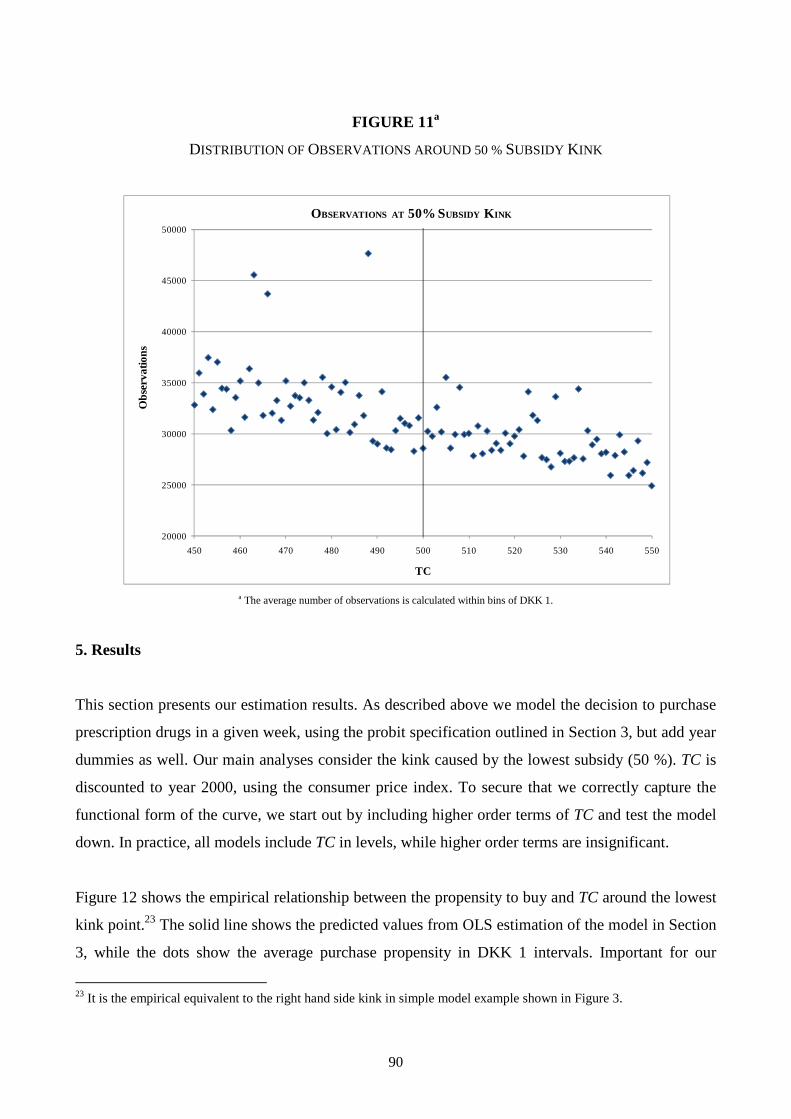
90
FIGURE 11a
DISTRIBUTION OF OBSERVATIONS AROUND 50 % SUBSIDY KINK
a The average number of observations is calculated within bins of DKK 1.
5. Results
This section presents our estimation results. As described above we model the decision to purchase
prescription drugs in a given week, using the probit specification outlined in Section 3, but add year
dummies as well. Our main analyses consider the kink caused by the lowest subsidy (50 %). TC is
discounted to year 2000, using the consumer price index. To secure that we correctly capture the
functional form of the curve, we start out by including higher order terms of TC and test the model
down. In practice, all models include TC in levels, while higher order terms are insignificant.
Figure 12 shows the empirical relationship between the propensity to buy and TC around the lowest
kink point.23 The solid line shows the predicted values from OLS estimation of the model in Section
3, while the dots show the average purchase propensity in DKK 1 intervals. Important for our
23 It is the empirical equivalent to the right hand side kink in simple model example shown in Figure 3.
20000
25000
30000
35000
40000
45000
50000
450 460 470 480 490 500 510 520 530 540 550
OBSERVATIONS AT 50% SUBSIDY K INK
Obs
erva
tions
TC

91
strategy, the figure indicates that there is a shift in the slope of the purchase propensity around the
50% subsidy kink point. This is the variation we are identifying price sensitivity off.
FIGURE 12a
a The average purchase propensity is calculated within bins of DKK 1. The solid line shows predicted values from OLS estimation of the model in Section 3.
Table 8 presents the results from the formal analyses for the 50% subsidy kink point.24 As
mentioned above, all standard errors are clustered at the individual level. The upper part of the table
shows the results, using the full set of products. The estimates are small and negative and in line
with those from the existing literature. The size of the estimates does vary somewhat with the
bandwidth: the estimate using a bandwidth of DKK 50 yields an elasticity of -0.09; a 10 % increase
in the price decreases the propensity to buy with 0.9 %. This estimate is significant at the 10 %
level, while the estimated elasticity using a DKK 25 bandwidth is larger in size (-0.25) and
significant at the 5 % level. The lower part of the table shows results when including covariates in
the analyses. We condition on the variables shown in Tables 5 and 6 above: Number of children,
labor income, degree of unemployment throughout the year, income, age, an indicator for more than
12 years of education, and time in weeks until end of personal subsidy year. The size of the
24 Results where we for example include both first and second order terms of TC are available on request.
PURCHASE PROPENSITY AT 50 % SUBSIDY K INK
0,1075
0,1125
0,1175
0,1225
0,1275
450 460 470 480 490 500 510 520 530 540 550
TC
Pur
chas
e P
rope
nsity

92
estimated elasticity using a DKK 25 bandwidth is reduced from -0.25 to -0.19 by this exercise, yet
the two estimates are not significantly different from each other. The result using a DKK 50
bandwidth is almost unchanged by the inclusion of covariates. Table A4 in Appendix A shows
these main results, both with and without conditioning set, for bandwidth choices ranging from
DKK 50 – DKK 5 in DKK 5 intervals.
5.1 Sensitivity analysis
As discussed above, it is unlikely that all individuals react similarly to price variation. This
subsection investigates whether the estimated parameters for the 50 % subsidy threshold vary across
subpopulations and investigates price sensitivity at the 75 % threshold. Table 9 shows the results
where we only include individuals who exclusively receive general subsidies. That is, we exclude
individuals who receive any additional subsidies as outlined in Section 2. This exercise reduces
sample sizes with around 50 %. Significance is, not surprisingly, affected by this, but the estimates
are similar to those using the full set of products. Thus there is no evidence that individuals who
receive additional subsidies are more or less sensitive to the price of prescription drugs compared to
individuals who receive further subsidies.25
25 As mentioned above, in a future version we will investigate the sensitivity of our results to the exclusion of individuals with private insurance. To some extent, the results of subgroup sensitivity analysis performed in this subsection could be driven by differences across groups in the propensity to sign up for private health insurance. For now, it is comforting to note that at least excluding individuals with access to additional public subsidies does not alter the results.
Treatment effect S.E. ImpliedAverage Purchase # #(*1,000) (*1,000) elasticity, ε price propensity Observations Individuals
(+/-) 50 DKK -0.11 0.06 -0.09 87.96 0.12 3,136,950 263,391 25 DKK -0.34 0.17 -0.25 85.47 0.12 1,558,687 171,564
Include covariates(+/-) 50 DKK -0.15 0.05 -0.12 87.96 0.12 3,136,950 263,391
25 DKK -0.26 0.15 -0.19 85.47 0.12 1,558,687 171,564 Treatment effecs and implied elasticit ies at DKK 500 kink. S.E. clustered by Person ID. Results are not sensitive to clustering. Average price is
that paid by consumers. Italic estimates are significant at the 10 % level, bold est imates are significant at the 5 % level.
TREATMENT EFFECTS AND IMPLIED ELASTICITIES, ALL PRODUCTS, 50 % SUBSIDY KINK, TC = DKK 500
TABLE 8

93
Secondly, we consider differences in price sensitivity by level of education and income in Tables 10
and 11, and the results are striking. We distinguish between high and low level of education (12
years or less education versus more than 12 years of education) and high and low income (less than
average income versus more than average income). Demand for prescription drugs for individuals
with lower levels of education is more responsive to the price than demand for individuals with
higher levels of education. Note that individuals with lower levels of education also pay a lower
average price. Similarly, demand for individuals with less than average income is more price
responsive than demand for individuals with higher than average income. There could be several
explanations for these patterns; apart from potential differences in preferences for health
investments, individuals with lower levels of income face tighter budget constraints, they could
have less information about the importance of taking a particular drug, or they could be treated
differently by doctors than individuals with higher socio-economic status. See for example
Simeonova (2008).
Treatment effect S.E. Implied Average Purchase # #(*1,000) (*1,000) elasticity, ε price propensity Observations Individuals
(+/-) 50 DKK -0.06 0.07 -0.06 96.44 0.09 1,550,985 135,670 25 DKK -0.37 0.21 -0.29 93.38 0.12 612,289 81,926
Include covariates(+/-) 50 DKK -0.04 0.03 -0.04 96.44 0.09 1,550,985 135,670
25 DKK -0.13 0.10 -0.10 93.38 0.12 612,289 81,926 Treatment effecs and implied elasticit ies at DKK 500 kink. S.E. clustered by Person ID. Results are not sensit ive to clustering. Average price is
that paid by consumers. Italic estimates are significant at the 10 % level, bold estimates are significant at the 5 % level.
50 % SUBSIDY KINK, TC = DKK 500, GENERAL SUBSIDY ONLY
TABLE 9TREATMENT EFFECTS AND IMPLIED ELASTICITIES, ALL PRODUCTS,
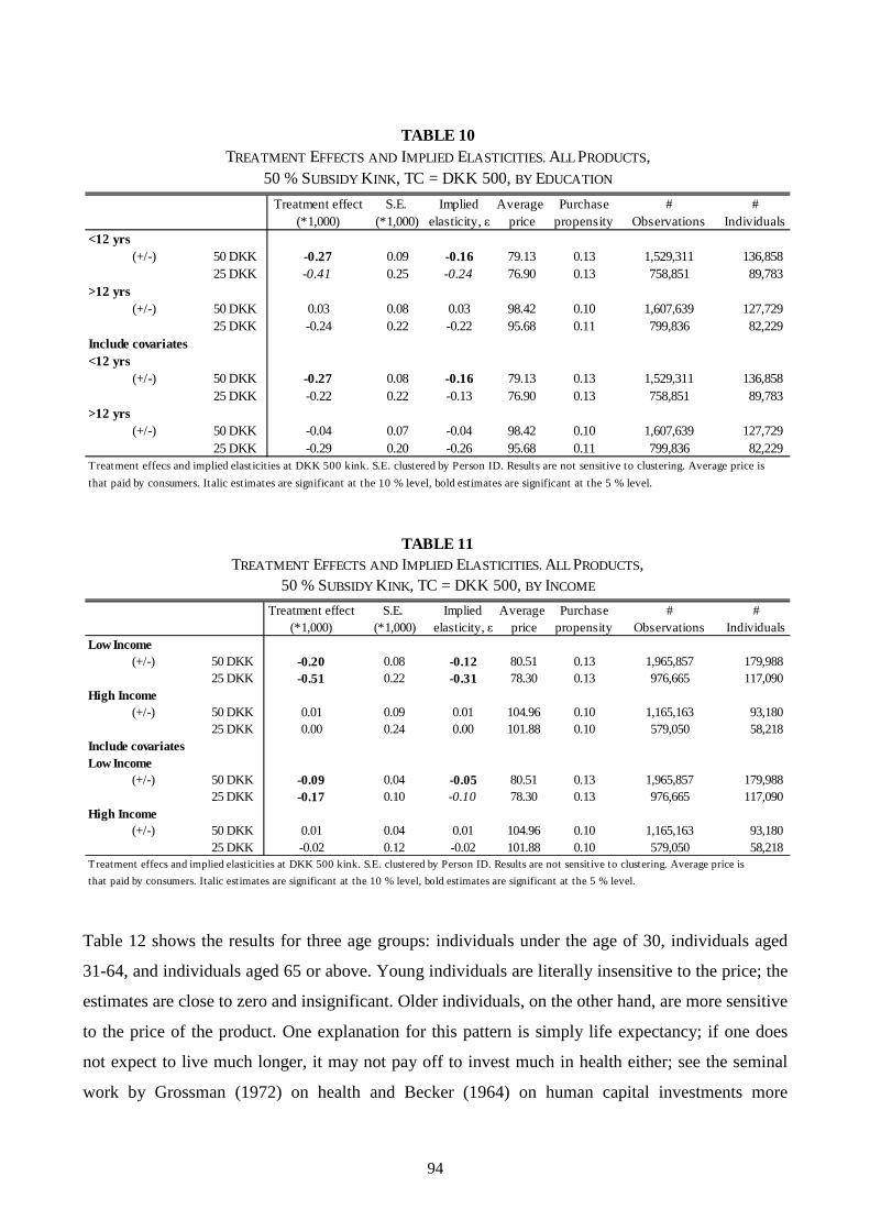
94
Table 12 shows the results for three age groups: individuals under the age of 30, individuals aged
31-64, and individuals aged 65 or above. Young individuals are literally insensitive to the price; the
estimates are close to zero and insignificant. Older individuals, on the other hand, are more sensitive
to the price of the product. One explanation for this pattern is simply life expectancy; if one does
not expect to live much longer, it may not pay off to invest much in health either; see the seminal
work by Grossman (1972) on health and Becker (1964) on human capital investments more
Treatment effect S.E. Implied Average Purchase # #(*1,000) (*1,000) elasticity, ε price propensity Observations Individuals
<12 yrs(+/-) 50 DKK -0.27 0.09 -0.16 79.13 0.13 1,529,311 136,858
25 DKK -0.41 0.25 -0.24 76.90 0.13 758,851 89,783 >12 yrs
(+/-) 50 DKK 0.03 0.08 0.03 98.42 0.10 1,607,639 127,729 25 DKK -0.24 0.22 -0.22 95.68 0.11 799,836 82,229
Include covariates<12 yrs
(+/-) 50 DKK -0.27 0.08 -0.16 79.13 0.13 1,529,311 136,858 25 DKK -0.22 0.22 -0.13 76.90 0.13 758,851 89,783
>12 yrs(+/-) 50 DKK -0.04 0.07 -0.04 98.42 0.10 1,607,639 127,729
25 DKK -0.29 0.20 -0.26 95.68 0.11 799,836 82,229 Treatment effecs and implied elast icit ies at DKK 500 kink. S.E. clustered by Person ID. Results are not sensitive to clustering. Average price is
that paid by consumers. Italic estimates are significant at the 10 % level, bold estimates are significant at the 5 % level.
TABLE 10TREATMENT EFFECTS AND IMPLIED ELASTICITIES, ALL PRODUCTS,
50 % SUBSIDY KINK, TC = DKK 500, BY EDUCATION
Treatment effect S.E. Implied Average Purchase # #(*1,000) (*1,000) elasticity, ε price propensity Observations Individuals
Low Income(+/-) 50 DKK -0.20 0.08 -0.12 80.51 0.13 1,965,857 179,988
25 DKK -0.51 0.22 -0.31 78.30 0.13 976,665 117,090 High Income
(+/-) 50 DKK 0.01 0.09 0.01 104.96 0.10 1,165,163 93,180 25 DKK 0.00 0.24 0.00 101.88 0.10 579,050 58,218
Include covariatesLow Income
(+/-) 50 DKK -0.09 0.04 -0.05 80.51 0.13 1,965,857 179,988 25 DKK -0.17 0.10 -0.10 78.30 0.13 976,665 117,090
High Income(+/-) 50 DKK 0.01 0.04 0.01 104.96 0.10 1,165,163 93,180
25 DKK -0.02 0.12 -0.02 101.88 0.10 579,050 58,218 Treatment effecs and implied elasticities at DKK 500 kink. S.E. clustered by Person ID. Results are not sensit ive to clustering. Average price is
that paid by consumers. Italic est imates are significant at the 10 % level, bold estimates are significant at the 5 % level.
TABLE 11TREATMENT EFFECTS AND IMPLIED ELASTICITIES, ALL PRODUCTS,
50 % SUBSIDY KINK, TC = DKK 500, BY INCOME

95
generally. Another explanation could be that the elderly population aged 65 or above also has lower
levels of income, though they also have higher accumulated wealth.
A fourth sensitivity analysis distinguishes between essential and other types of drugs (the
complement set). Essential drugs are defined as “medications that prevent deterioration in health or
prolong life and would not likely be prescribed in the absence of a definitive diagnosis”, Tamblyn et
al. (2001), page 422. See Table B2 in Appendix B for the list of drugs included in the essential
category. As expected, demand for essential drugs is less price responsive than demand for other
types of drugs. Note though that the complement set of drugs may also include drugs that in some
cases – but not always – fit the definition of essential drugs. One example is antibiotics.
Treatment effect S.E. Implied Average Purchase # #(*1,000) (*1,000) elasticity, ε price propensity Observations Individuals
< 30 years(+/-) 50 DKK 0.00 0.14 0.00 92.08 0.08 353,920 26,698
25 DKK -0.02 0.39 -0.03 89.89 0.08 176,284 16,315 30-64 years
(+/-) 50 DKK -0.07 0.07 -0.07 95.19 0.11 1,945,452 155,255 25 DKK -0.34 0.20 -0.29 92.47 0.11 966,466 100,077
65+ years(+/-) 50 DKK -0.27 0.12 -0.13 76.12 0.16 837,578 86,483
25 DKK -0.19 0.34 -0.09 73.95 0.16 415,937 57,134 Include covariates< 30 years
(+/-) 50 DKK -0.05 0.14 -0.06 92.08 0.08 353,920 26,698 25 DKK -0.02 0.38 -0.02 89.89 0.08 176,284 16,315
30-64 years(+/-) 50 DKK -0.12 0.07 -0.11 95.19 0.11 1,945,452 155,255
25 DKK -0.39 0.18 -0.34 92.47 0.11 966,466 100,077 65+ years
(+/-) 50 DKK -0.30 0.11 -0.14 76.12 0.16 837,578 86,483 25 DKK -0.04 0.31 -0.02 73.95 0.16 415,937 57,134
Treatment effecs and implied elast icit ies at DKK 500 kink. S.E. clustered by Person ID. Results are not sensit ive to clustering. Average price is
that paid by consumers. Italic est imates are significant at the 10 % level, bold est imates are significant at the 5 % level.
TABLE 12TREATMENT EFFECTS AND IMPLIED ELASTICITIES, ALL PRODUCTS,
50 % SUBSIDY KINK, TC = DKK 500, BY AGE

96
We finally investigate the 75 % subsidy kink. The estimated treatment effects are still negative and
slightly smaller in size. Only the result for the DKK 50 bandwidth is statistically significant.
Because of more limited sample sizes (the number of observations is reduced to around 40 % when
we move from the 50 % subsidy kink to the 75 % subsidy kink) and a lower change in the subsidy
at the higher kink, we refrain from performing subgroup specific analyses.
Our results are not directly comparable to those from the RAND HIE (see Manning et al. (1987)
and Newhouse (1993)) since that study considered – for the non-aged population – total health care
utilization and not only prescription drugs. Our results, on the other hand, are local in the sense that
they are estimated around the 50 % subsidy kink point. Using a similarly aged population, our
Treatment effect S.E. Implied Average Purchase # #(*1,000) (*1,000) elasticity, ε price propensity Observations Individuals
Essential(+/-) 50 DKK 0.00 0.03 -0.01 101.55 0.03 3,136,950 263,391
25 DKK -0.12 0.09 -0.35 99.29 0.03 1,558,687 171,564 Other
(+/-) 50 DKK -0.12 0.05 -0.12 82.39 0.08 3,136,950 263,391 25 DKK -0.22 0.14 -0.21 79.84 0.08 1,558,687 171,564
Include covariatesEssential
(+/-) 50 DKK -0.02 0.03 -0.05 101.55 0.03 3,136,950 263,391 25 DKK -0.09 0.08 -0.27 99.29 0.03 1,558,687 171,564
Other(+/-) 50 DKK -0.15 0.02 -0.14 82.39 0.08 3,136,950 263,391
25 DKK -0.17 0.13 -0.16 79.84 0.08 1,558,687 171,564 Treatment effecs and implied elasticit ies at DKK 500 kink. S.E. clustered by Person ID. Results are not sensitive to clustering. Average price is
that paid by consumers. Italic estimates are significant at the 10 % level, bold est imates are significant at the 5 % level.
TABLE 13TREATMENT EFFECTS AND IMPLIED ELASTICITIES
50 % SUBSIDY KINK, TC = DKK 500, BY DRUG TYPE
Treatment effect S.E. ImpliedAverage Purchase # #(*1,000) (*1,000) elasticity, ε price propensity Observations Individuals
(+/-) 50 DKK -0.43 0.20 -0.15 60.76 0.17 1,289,790 168,086 25 DKK -0.45 0.56 -0.16 59.76 0.17 639,732 104,591
Include covariates(+/-) 50 DKK -0.50 0.19 -0.18 60.76 0.17 1,289,790 168,086
25 DKK -0.47 0.53 -0.17 59.76 0.17 639,732 104,591 Treatment effecs and implied elasticit ies at DKK 1200 kink. S.E. clustered by Person ID. Results are not sensit ive to clustering. Average price is the that
paid by consumers. Italic est imates are significant at the 10 % level, bold estimates are significant at the 5 % level.
TABLE 14TREATMENT EFFECTS AND IMPLIED ELASTICITIES, ALL PRODUCTS,
75 % SUBSIDY KINK, TC = DKK 1200

97
results are, nonetheless, fairly close in size to those from the RAND HIE. Our study does suggest
that the elderly population is more responsive to the price than the non-elderly, and the results are in
line with the Canadian study by Contoyannis et al. (2005) who find moderate price elasticities (-
0.12 to -0.16) as well as with the US study by Chandra et al. (2010) (elasticities -0.08 to -0.15).26 As
suggested by Tamblyn et al. (2001) and also investigated by Chandra et al. (2010), we find that
demand for essential drugs is less sensitive to the price than less essential drugs.
6. Conclusion
We estimate price sensitivity of demand for prescription drugs, exploiting truly exogenous variation
in the price that stems from a kinked reimbursement scheme. Within a unifying framework, we are
able to address this question for different subpopulations and types of drugs. We find that demand is
indeed sensitive to the price, although estimated implied elasticities are small; the overall elasticity
ranges between -0.09 and -0.25 for individuals who have, so far, bought prescription drugs worth at
least DKK 500 (€ 70) in a given 12-month period. There is important variation in which subgroups
are affected by the price of prescription drugs. Individuals with lower income and lower education
are, despite (or maybe because of) their lower average health capital, more sensitive to the price of a
product. The same is true for the elderly population. Thus, policy makers should be aware that
reductions in subsidies for these groups are likely to result in lower consumption and, presumably,
worse health outcomes. Along similar lines, lower consumption of prescription drugs may increase
the take-up of inpatient and outpatient cases; see for example Chandra et al. (2010) and Gaynor, Li,
and Vogt (2006) for evidence of this behavior. Finally, essential drugs that surely prevent
deterioration of health and keep patients alive have, as expected, much lower associated average
price sensitivity than other drugs.
26 Chandra et al. (2010) argue that the products with elastic demand are those for which consumers can easily substitute into other treatments.
98
Literature
Altonji, J. G. and R. L: Matzkin (2005): Cross Section and Panel Data Estimators for Nonseparable
Models with Endogenous Regressors, Econometrica 73, 1053-1102.
Becker, G. S. (1964): Human Capital. New York: Columbia University Press.
Card, D., D. S. Lee and Z. Pei (2009), “Quasi-Experimental Identification and Estimation in the
Regression Kink Design”, Princeton University, WP # 553.
Chandra, A., J. Gruber, J. and R. McKnight (2010): “Patient Cost - Sharing and Hospitalization
Offsets in the Elderly”, American Economic Review 100, 193-213.
Chetty, R., J. N. Friedman, T. Olsen, and L. Pistaferri (2009): The Effect of Adjustment Costs and
Institutional Constraints on Labor Supply Elasticities: Evidence from Denmark. Mimeo, Harvard
University.
Contoyannis, P., J. Hurley, P. Grootendorst, S. Jeon and R. Tablyn (2005): “Estimating the price
elasticity of expenditure for prescription drugs in the presence of non-linear price schedules: an
illustration from Quebec, Canada”, Health Economics 14, 909-923.
Dynarski, S., J. Gruber and D. Li (2009): Cheaper by the dozen: using sibling discounts at catholic
schools to estimate the price elasticity of private school attendance. NBER WP # 15461.
Florens, J. P., J. J. Heckman, C. Meghir and E. J. Vytlacil (2008), ”Identification of Treatment
Effects Using Control Functions in Models with Continuous, Endogenous Treatment and
Heterogeneous Effects”, Econometrica 76, 1191-1206.
Gaynor, M., J. Li and W. B. Vogt (2007): Is drug coverage a free lunch? Cross-price elasticities and
the design of prescription drug benefits, NBER WP #12758.
99
Goldman, D. P., G. F. Joyce, J. J. Escarce, J. E. Pace, M. D. Solomon, M. Laouri, P. B. Landsman,
and M. Teutsch (2004): “Pharmacy Benefits and the Use of Drugs by the Chronically Ill”, Journal
of the American Medical Association 291, 2344-2350.
Grossman, M. (1972): “On the Concept of Health Capital and the Demand for Health”, Journal of
Political Economy 80, 223-255.
Guryan, J. (2003): Does Money Matter: Regression-Discontinuity Estimates from Education
Finance Reform in Massachusetts”, NBER WP # 8269.
Hahn, J., P. Todd and W. van der Klaauw (2001): “Identification and Estimation of Treatment
Effects with a Regression-Discontinuity Design”, Econometrica 69, 201-209.
Keeler, E. B., J. P. Newhouse, and C. E. Phelps (1977): “Deductibles and the Demand for Medical
Care Services: the Theory of a Consumer Facing a Variable Price Schedule under Uncertainty”,
Econometrica 45, 641-655.
Landsman, P. B., W. Yu, X. F. Liu, S. M. Teutsch and M. L. Baerger (2005): Impact of 3-Tier
Pharmacy Benefit Design and Increased Consumer Cost-sharing on Drug Utilization. The American
Journal of Managed Care 11, 621-628.
Lee, D. S. and T. Lemieux (forthcoming): Regression Discontinuity Designs in Economics, Journal
of Economic Literature.
Manning, W. G., J. P. Newhouse, N. Duan, E. B. Keeler, A. Leibowitz, and M. S. Marquis (1987):
Health Insurance and the Demand for Medical Care: Evidence from a Randomized Experiment. The
American Economic Review 77, 251-277.
Moffitt, Robert (1990): The Econometrics of Kinked Budget Constraints. Journal of Economic
Perspectives 4, 119-139.

100
Newhouse, J. (1993): Free for All: Lessons from the RAND Health Insurance Experiment.
Cambridge, MA. Harvard University Press.
Nielsen, H. S., C. Taber and T. Sørensen (2010): Estimating the Effect of Student Aid on College
Enrollment: Evidence from a Government Grant Policy Reform. American Economic Journal:
Economic Policy 2, (May 2010): 185-215.
OECD (2009): Health at a Glance 2009: OECD Indicators.
Rothstein, J. and C. Rouse (2007): Constrained after College: Student Loans and Early Career
Occupational Choices, NBER WP #13117.
Saez, E. (2009): Do Tax Filers Bunch at Kink Points? Evidence, Elasticity Estimation, and Salience
Effects. Mimeo, University of California at Berkeley.
Simeonova, E. (2008): Doctors, Patients, and the Racial Mortality Gap: What are the Causes?
Mimeo, University of Stockholm.
Skipper, N. (2009): On Utilization and Stockpiling of Prescription Drugs when Co-payments
Increase: Heterogeneity Across Types of Drugs. Mimeo, Aarhus University.
Tamblyn, R., R. Laprise, J. A. Hanley et al. (2001): Adverse Events Associated with Prescription
Drug Cost-Sharing among Poor and Elderly Persons, Journal of the American Medical Association
285, 421-429.

101
Appendix A
TABLE A1
As can be seen from Table A1, the type of drug most frequently used is psycholeptic drugs
(antipsychotics). The second most frequently purchased type of drugs belongs to the analgesics
category (pain relievers). This category covers products for severe pain (e.g. morphine) to over-the-
counter products such as Panodil/Tylenol (mild pain relievers would qualify for conditional
subsidy). In third place are sex hormones and modulators of the genital system.
ATC-group Count Percent
N05 2,538,410 9.3%
N02 2,515,002 9.2%
G03 1,883,471 6.9%
J01 1,730,247 6.3%
R03 1,720,373 6.3%
M01 1,387,090 5.1%
C03 1,216,623 4.4%
N06 1,213,187 4.4%
S01 1,056,132 3.9%
C09 969,884 3.5%
A02 884,389 3.2%
C07 727,287 2.7%
B01 720,792 2.6%
A10 691,968 2.5%
C08 654,489 2.4%
D07 603,136 2.2%
C01 537,727 2.0%
A12 441,297 1.6%
C10 437,885 1.6%
R05 421,115 1.5%
THE 20 MOST FREQUENTLY USED THERAPEUTIC GROUPS
Name
Statist ics Denmark. Purchases in period March 1st 2000-2003, age 18 and above, 20% sample.
Agents that exert an action on the renin-angiotensin system
Agents that exert an action on acid related disorders
Beta blocking agents
Anti-thrombotic drugs
Obstructive airway disease agents
Mineral supplements
Lipid modifying agents
Ophthalmologics
Anti-diabetics
Calcium channel blockers
Cough and cold preparations
Psycholeptics
Analgesics
Sex hormones and modulators of the genital system
Antibacterial agents for systemic use
Corticosteroids for dermatological use
Cardiac therapy
Anti-inflammatory and anti-rheumatic agents
Diuretics
Psycho analeptics

102
TABLE A2
Table A2 shows therapeutic groups by expenditure shares. Here, obstructive airway disease agents
(asthma medicine) dominate with psychoanaleptics (anti-depressants and ADHD drugs) and
analgesics in second and third place.
Finally, Table A3 shows the 20 most frequently sold products. Here, we exploit the full ATC-code
level. As can be seen, phenoxymethylpenicillin (penicillin) is the single most prescribed drug,
claiming about 2.5 % of total sales. The second most sold product is paracetamol, which is a pain
reliever. In third and fourth place are ibuprofen (used for anti-inflammatory and anti-rheumatic
purposes) and Tramadol (a pain-reliever).
ATC-group Totalb
Percent
R03 583.21 9.4%
N06 540.92 8.7%
N02 485.86 7.9%
N05 416.05 6.7%
C09 384.01 6.2%
A02 363.43 5.9%
G03 347.65 5.6%
C10 294.26 4.8%
C08 285.55 4.6%
M01 220.28 3.6%
N03 196.26 3.2%
A10 190.24 3.1%
J01 181.32 2.9%
G04 144.35 2.3%
C07 127.90 2.1%
C03 126.18 2.0%
S01 122.16 2.0%
B01 94.63 1.5%
N04 74.03 1.2%
C01 72.45 1.2%
Beta blocking agents
Diuretics
b In million DKK. 2000 prices.
Ophthalmologics
Anti-thrombotic drugs
Anti-Parkinson drugs
Cardiac therapyStatist ics Denmark. Purchases in period March 1st 2000-2003, age 18 and above, 20% sample.
Antiepileptics
Anti-diabetics
Antibacterial agents for systemic use
Urologicals
Sex hormones and modulators of the genital system
Lipid modifying agents
Calcium channel blockers
Anti-inflammatory and anti-rheumatic agents
Analgesics
Psycholeptics
Agents that exert an action on the renin-angiotensin system
Agents that exert an action on acid related disorders
THERAPEUTIC GROUPS BY EXPENDITURES
Name
Obstructive airway disease agents
Psycho analeptics

103
TABLE A3
ATC Count Percent Name
J01CE02 701,131 2.6%N02BE01 698,499 2.6%M01AE01 530,563 1.9%N02AX02 503,580 1.8%C03AB01 495,914 1.8%C03CA01 461,611 1.7%B01AC06 406,307 1.5%G03AA10 402,766 1.5%A12BA01 387,657 1.4%N06AB04 375,156 1.4%N05BA01 371,741 1.4%N05CF01 362,669 1.3%C07AB02 354,240 1.3%C08CA01 322,811 1.2%N05BA04 305,946 1.1%M01AB05 294,313 1.1%G03CA03 280,244 1.0%R03BA02 254,655 0.9%R03AC02 251,607 0.9%R03AC03 249,014 0.9%
Salbutamol
TerbutalineStatist ics Denmark. Purchases in period March 1st 2000-2003, age 18 and above, 20% sample.
Metoprolol
Amlodipin
Oxazepam
Diclofenac
Estradiol
Budesonid
Potassium chloride
Citalopram
THE 20 MOST SOLD PRODUCTS BY ATC-CODE
Diazepam
Zopiclone
Phenoxymethylpenicillin
Paracetamol
Ibuprofen
Tramadol
Bendroflumethiazid and potassium
Furosemide
Acetylsalicylic acid
Gestodene and estrogen

104
Treatment effect S.E. Implied(*1,000) (*1,000) elasticity, ε
(+/-) 50 DKK -0.11 0.06 -0.0945 DKK -0.13 0.07 -0.1040 DKK -0.20 0.08 -0.1535 DKK -0.34 0.10 -0.2530 DKK -0.52 0.13 -0.3825 DKK -0.34 0.17 -0.2520 DKK -0.28 0.23 -0.2015 DKK -0.52 0.35 -0.3810 DKK -0.13 0.65 -0.095 DKK 1.51 1.84 1.05
Include all covariates(+/-) 50 DKK -0.15 0.05 -0.12
45 DKK -0.18 0.06 -0.1440 DKK -0.29 0.07 -0.2235 DKK -0.40 0.09 -0.2930 DKK -0.50 0.11 -0.3625 DKK -0.26 0.15 -0.1920 DKK -0.24 0.21 -0.1715 DKK -0.57 0.32 -0.4110 DKK -0.40 0.59 -0.285 DKK 0.60 1.66 0.42
Include all covariates OLS
(+/-) 50 DKK -0.18 0.05 -0.1345 DKK -0.24 0.06 -0.1840 DKK -0.38 0.08 -0.2835 DKK -0.50 0.09 -0.3730 DKK -0.61 0.12 -0.4425 DKK -0.37 0.15 -0.2620 DKK -0.36 0.21 -0.2615 DKK -0.75 0.33 -0.5410 DKK -0.49 0.62 -0.355 DKK 0.94 1.75 0.65
Treatment effecs and implied elasticit ies at DKK 500 kink. S.E. clustered by Person ID.
Results are not sensit ive to clustering. Average price is the that paid by consumers. Italic
estimates are significant at the 10 % level, bold estimates are significant at the 5 % level.
TABLE A4TREATMENT EFFECTS AND IMPLIED ELASTICITIES, ALL PRODUCTS,
50 % SUBSIDY KINK, TC = DKK 500

105
Appendix B
Essential drugs: Insulin, anticoagulants, angiotensin-converting enzyme inhibitors,lipid-reducing medication, antihypertensives, furosemide, B-blockers,antiarrhythmics, aspirin, antiviral medication, thyroid medication, neuroleptics, antidepressants, anticonvulsants, antiparkinsonian drugs,prednisone, β-agonists, inhaled steroids, chloroquines, primaquines,and cyclosporine.
ESSENTIAL DRUGS
TABLE B1

106

107
CHAPTER 3
Income and the Use of Prescription Drugs
for Near Retirement Individuals

108

† Department of Economics, University of Copenhagen, Øster Farimagsgade 5, building 26, DK-1353 Copenhagen. Email: [email protected]. *School of Economics and Management, Aarhus University, Bartholins Allé 10, Building 1323, 3, DK-8000 Aarhus. Email: [email protected] 109
Income and the Use of Prescription Drugs
for Near Retirement Individuals
Søren Leth-Petersen†, Niels Skipper*
November 2010
Abstract:
Understanding how demand for prescription drugs responds to changes in income is important
for assessing the welfare consequences of reforms affecting income. This becomes more
imminent as age progresses, because the use of prescription drugs and the associated budgetary
burden increases dramatically from about age 55. In this paper we estimate how demand for
prescription drugs varies with income for a sample of near retirement individuals. Estimating the
prescription drug demand response to income changes is complicated because an important
explanatory variable, the health capital, is unobserved, and because demand is potentially
dynamic, for example because some drugs are habitual. The analysis is based on a novel panel
data set with information about purchase of prescription drug demand for a very large number of
Danish individuals over the period 1995-2003. Our preferred model that takes into account the
aforementioned complications performs better in an external validation test than models that can
be estimated on cross section data. Results indicate that demand does respond to variations in
income and that reforms affecting income therefore will affect the use of prescription drugs.
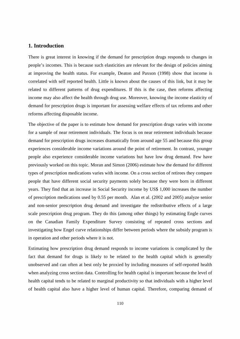
110
1. Introduction
There is great interest in knowing if the demand for prescription drugs responds to changes in
people’s incomes. This is because such elasticities are relevant for the design of policies aiming
at improving the health status. For example, Deaton and Paxson (1998) show that income is
correlated with self reported health. Little is known about the causes of this link, but it may be
related to different patterns of drug expenditures. If this is the case, then reforms affecting
income may also affect the health through drug use. Moreover, knowing the income elasticity of
demand for prescription drugs is important for assessing welfare effects of tax reforms and other
reforms affecting disposable income.
The objective of the paper is to estimate how demand for prescription drugs varies with income
for a sample of near retirement individuals. The focus is on near retirement individuals because
demand for prescription drugs increases dramatically from around age 55 and because this group
experiences considerable income variations around the point of retirement. In contrast, younger
people also experience considerable income variations but have low drug demand. Few have
previously worked on this topic. Moran and Simon (2006) estimate how the demand for different
types of prescription medications varies with income. On a cross section of retirees they compare
people that have different social security payments solely because they were born in different
years. They find that an increase in Social Security income by US$ 1,000 increases the number
of prescription medications used by 0.55 per month. Alan et al. (2002 and 2005) analyze senior
and non-senior prescription drug demand and investigate the redistributive effects of a large
scale prescription drug program. They do this (among other things) by estimating Engle curves
on the Canadian Family Expenditure Survey consisting of repeated cross sections and
investigating how Engel curve relationships differ between periods where the subsidy program is
in operation and other periods where it is not.
Estimating how prescription drug demand responds to income variations is complicated by the
fact that demand for drugs is likely to be related to the health capital which is generally
unobserved and can often at best only be proxied by including measures of self-reported health
when analyzing cross section data. Controlling for health capital is important because the level of
health capital tends to be related to marginal productivity so that individuals with a higher level
of health capital also have a higher level of human capital. Therefore, comparing demand of

111
individuals with high income with that of individuals with low income in order to estimate Engle
curves is likely to (also) reflect selection effects. Moreover, the use of prescription drugs is likely
to be endogenous to the extent that consuming drugs improves health and thereby earnings
capacity and income. Another issue relates to the dynamic aspects of drug demand. Some drugs
are habitual and the consumption may be the consequence of treatments that extend beyond the
period for which the data is collected, typically one year. At best, the above mentioned papers
take in to account one of these issues. We argue that it is crucial to control for all of them when
modeling the dependence of demand for prescription drugs on income. In fact leaving out one of
these elements from the analysis can lead to seriously biased Engle curve estimates.
The analysis presented in this paper is based on a panel data set with information about 20% of
the Danish population under the age of 70. This data set has some unique features that are crucial
in this context. Most importantly, and unlike any other data set that we know of, it holds person
level panel information about demand for prescription drugs for the period 1995-2003. This
enables us to model the dynamic structure of demand and to take account of person-level fixed
unobserved factors as well as correlation between income and the idiosyncratic error term.
Moreover, covering 20% of the Danish population the data set is very large compared to
expenditure surveys or other data sets with information about the demand for prescription drugs.
This enables us to consider prescription drug demand for subsets of the population without
relying on small samples. We use this feature to illustrate that the effect of income on the
demand for prescription drugs can vary significantly across different levels of income.
In the main analysis we focus on persons aged 55-651, i.e., persons near retirement. The results
show a strong relationship between income and the demand for prescription drugs when
estimated on a cross section. However, taking into account the dynamic structure of demand as
well as fixed factors controlling for individual specific levels of health capital is very important
in this context. Applying an appropriate panel data model weakens this relationship considerably.
This suggests that Engle curve relationships estimated off cross section data may lead to biased
estimates of the Engle curve relationship and that caution is warranted when giving such
estimates a behavioral interpretation, i.e., as an estimate of the demand response to a change in
1 Observations for age groups 66-69 are reserved for an external validation exercise where the estimated model’s ability to capture the adjustment in demand following the change in income from age 66 to 68 is investigated.

112
income. This knowledge is essential for policy makers trying to design policies that affect the
level of disposable income. If polices are based on relationships estimated on cross section data,
then the effects on demand from welfare reforms can appear substantial when they in fact are
small. Results from this study, however, still suggest that reforms affecting income, for example
reforms of the public pension provision, will affect the demand for prescription drugs.
The remainder of the paper is organized as follows. In the next section we sketch the empirical
problem and suggest a solution to it. Section 3 presents the data and shows how demand differs
between young and old persons by estimating nonparametric Engle curves on cross sections from
our gross data set. Section 4 presents a multivariate analysis in which we try to take in to account
potentially confounding factors. In this section we also show how the results differ between
young and old persons. In section 5 we attempt to validate our model for the near-retirement
sample by checking its ability to predict the adjustment in demand following the first receipt
from a universal government public pension scheme that is awarded irrespectively of whether the
individual has labor income. The idea is that this leads to an exogenous change in income that is
arguably unrelated to the development in health status. Section 6 sums up and concludes.
2. Method
There are several complications associated with estimating Engle curves for prescription drug
demand. First, demand is potentially driven by unobserved factors that we refer to as health
capital, cf. Grossman (1972). More health capital leaves the individual more resistant to adverse
health events and individuals equipped with more health capital are assumed to have a lower
level of consumption of prescription drugs. The stock of health capital is likely heterogeneous
across the population where some individuals are generally equipped with a high level of health
capital and others with a low level of health capital. In general, health capital will be non-
separable from human capital so that an adverse shock to the health capital also produces an
adverse shock to earnings. The effects of such adverse shocks can be mitigated by consuming
drugs that restore the health capital and stimulate productivity again. Another complication
relates to the potential dynamic aspects of drug demand. Drug demand potentially follows a
dynamic process because demand is habitual, but it can also reflect that the data are collected
over a time frame that does not match the time frame of the treatment. This occurs, for example,
113
when data are collected from January to December but the treatment program runs from
November to March. In this section we formulate a demand model that can handle these
concerns.
Consider the following demand function.
��� � �� � ���� � ����� � � ���� � ����� � �� � ��� (1)
where � � 1, … , � is the person identifier and � identifies the period of observation. ��� is the
share of income allocated to prescription drugs for individual � in year �, and ��� is the
expenditure share for person � measured in the previous period. ��� is the natural log of
disposable income. Following the standard in the demand literature we include a quadratic term
in log-income, Banks, Blundell and Lewbel (1997), to allow the Engle curve to be nonlinear. ��
is a vector of control variables including age, sex, marital status, number of children,
immigrant/native, education, occupation and geographical location. ��, �, ��, � , �� are
parameters to be estimated, but the focus in this paper is on the estimation of the income
response, and ��, � are therefore the parameters of interest in this study. Prices are subsidized
according to a complicated scheme that is generally independent of the level of income, and we
therefore ignore price effects2, see Simonsen et al. (2010). �� is an unobserved effect that is
specific to person �, and ��� is an error term that may vary across time periods and individuals.
We think of �� as capturing innate unobserved health or the part of the health capital that is
approximately fixed over the time span where we observe a person in our data set. Because
health capital is potentially nonseparable from human capital, �� is potentially correlated with ���
and our estimation method should address this. ��� includes unanticipated adverse health shocks.
An adverse health shock can generate a drop in income. The consumption of drugs on the other
hand can help restore the income level. ��� is therefore potentially correlated with ���. Estimating
2 Income-tested subsidies are granted by municipalities. The empirical analysis is insensitive to exclusion of
individuals receiving these subsidies. Additionally, in 2000, the subsidy scheme was reformed, so as to increase co payment. This affected people with low levels of prescription drug use most. In section 4 we shall perform a sensitivity check so as to make sure that this reform does not bias the results.

114
(1) by methods assuming orthogonality of the regressors is therefore not likely to produce
consistent estimates of �, ��, � . Moreover, the fact that ��� � �� � ����� � ����� �
� ���� � ����� � �� � ��� implies that �������, ��� � 0 in (1). Estimating the parameters
of (1) by OLS will therefore produce biased estimates not only of ��, � but also of � if �� is an
important factor in explaining ���.
To address these problems, we exploit the panel structure of the data and invoke the assumption
that �������, ����� � 0, � 1, … , ! " 1. This assumption is testable and it allows us to define a
set of instrumental variables that enable us to solve the problems associated with estimating (1).
Consider first the solution to the problem associated with estimating �. Note that
�������, ��� � 0 but ����∆���� , ��� � 0, $ 1. This suggests that ∆���� , $ 1 can be used as
instrumental variables for ��� in equation (1). Moreover note that ������� , ���� % 0 and
������� , ��� % 0 but that ����∆���� , ���� � ����∆���� , ��� � 0, $ 1. This suggest that
∆���� , $ 1 can be used as instrumental variables for ���.3
An alternative approach to addressing the problems associated with estimating the parameters of
(1) starts out solving the endogeneity problems arising because of the unobserved individual
specific effect ��. To do this, consider a first differenced version of (1)
∆��� � �� � �∆��� � ��∆��� � � ∆���� � ��∆��� � ∆��� (2)
In equation (2) still ����∆���, ∆���� � ����∆���, ∆���� � "�������� � & 0, and OLS on
(2) will still produce biased instruments. � can be consistently estimated by applying GMM/IV
using ����, � 2, … , ! " 2 as an instrument for ∆���. This follows the insights of Andersen
and Hsiao (1981) and Arellano and Bond (1991). We still need to accommodate the potential
endogeneity of ∆��� (and ∆���� ). This arises because:
3 A static demand relation with a linear Engle curve is nested in (1). In the result section we shall estimate such a
version of the model and compare its performance with the performance of (1) taking into account the endogeneity
of ���, ���, and ���� .

115
�������, ���� % 0 ( ����∆���, ∆���� � ������� , ���� � �������, ���� % 0
(and correspondingly for ∆���� ). We note that �������, ����� � �������, ����� � 0, �
2, … , ! " 2, and that income lagged twice or more therefore can be used as instruments for ∆���.
Arellano and Bover (1995) and Blundell and Bond (1998) suggest combining equations in levels,
(1), and equations in first differences, (2), in order to obtain a more efficient estimator. When the
autoregressive parameter is close to unity, i.e., the series is highly persistent, the lagged levels
become weak instruments in the differenced equations and yields biased estimates. Further, if the
variance of the individual fixed effect is large relative to that of the idiosyncratic error-term,
using only equations in first differences will yield biased estimates. Even for low values of the
autoregressive parameter, Monte Carlo simulations have shown that combining equations in
differences and levels implies significant efficiency gains; see Blundell and Bond (1998). Our
preferred estimator does exactly that4.
3. Data
We use administrative data provided by Statistics Denmark. The data set contains information
about a random sample of 20% of all Danish individuals in the period from 1995-2003. We
construct a balanced panel of individuals aged 18 to 69 including 681,837 individuals. In the
estimation part of the paper we focus on individuals between 55 and 65 years. 203,911 people in
the data set are aged 55-65 at some point in the panel. For each individual in the sample we know
the complete history of prescription drug purchases including date, prices etc. These data are
augmented with socio-economic information on age, sex, marital status, number of children,
immigrant/native, education, occupation and geographical location. The data set has one
shortcoming: it does not hold information on diagnosis or other types of in-or out-patient care.
4 One additional complication is that the dependent variable is censored at zero since some persons do not consume
drugs. Not taking censoring into account can be associated with inconsistent estimates. No estimator exists that simultaneously handles the endogeneity problems presented above while addressing the censoring issue. In section 5 we show evidence that the censoring problem is likely to be less important than the endogeneity problems, and we therefore proceed ignoring the censoring problem.

116
Descriptive Statistics
In table 1, descriptive statistics on a subset of the variables in the data set is presented. There are
marginally more women than men in the 55-65 age brackets as well as for the full sample. The
mean income for the full sample is DKK 255,058 and DKK 246,532 for the 55-65 year olds.
[Insert table 1 here]
In figure 1, a local polynomial regression of the drug expenditure share on age is depicted. As
can be seen, there is a strong, positive relationship between the two. This may be explained by a
deteriorating health status at old age, but as figure 2 shows, the average income is also falling
from age 60 and onwards. That is, this does not necessarily imply that the elderly consume more
drugs, only that they allocate a larger fraction of their income to drug consumption. Inspection of
the actual levels (not reported) reveals that demand is quantitatively increasing markedly from
around age 50.
[Insert figure 1 here]
[Insert figure 2 here]
The non-parametric Engel curve for total prescription drug consumption is graphed in figure 3.
As can be seen, there is a negative, monotonic relationship between the expenditure share and
income.
[Insert figure 3 here]
Note that a quadratic form seems to be able to capture the nonlinearities in drug demand. Given
that the elderly have a higher average expenditure share, the Engel curve relationship might
differ over age groups. In figure 4, two separate Engel curves are depicted: one for individuals
below 55 (‘young’) and one for individuals aged 55 or above (‘old’). The shapes of the two
relations are very similar, but the levels are different (note the different scales). This suggests
that the older part of the age distribution reacts more to income changes.5
[Insert figure 4 here]
5 Deaton and Paxson (1998) also find that the income-health correlation becomes stronger as age progresses.

117
4. Results
The estimation results for the sample of the 55 to 65 year-olds are reported in table 2. Columns
(1) and (2) are OLS estimations of the Engel curves. A linear income term is included in (1), and
income squared is included in (2). Both show a negative relationship between income and the
expenditure share just as we found in the non-parametric Engel curve in figure 3. Columns (3)
and (4) are the same as (1) and (2) but with income being treated as endogenous. Lagged
differences of the endogenous explanatory variable are used as instruments; see section 2. In the
linear case, treating income as endogenous does not affect the parameter estimates. When we
include income squared, however, treating income as endogenous reduces the point estimates to
both income terms. Note that the test of the overidentifying restrictions is rejected neither in (3)
nor (4) at the usual levels of significance, suggesting that instruments are valid.
[Insert table 2 here]
Column (5) holds the OLS results for the estimation with income, income squared and a lagged
dependent variable as key explanatory variables. When compared to (2), including the lagged
dependent variable reduces the numerical size of the point estimates of the income terms to about
the half. The AR parameter is 0.62 indicating a high degree of state dependence. The OLS
estimate of the AR parameter is known to be upward biased, Bond (2002). The within groups
estimate of the AR parameter in column (6) is 0.12. This estimate is downwards biased, and so
the true degree of persistence in demand is bounded by the estimates presented in columns (5)
and (6). In any case, estimating the relation by OLS or within groups produces biased estimates
of the AR parameter as well as the coefficients to the income terms.
The results for the GMM-SYS estimator that takes into account the endogeneity of the lagged
dependent variable but still treating income as exogenous is presented in column (7) where
��,��, ��,� , ��,�� are used as instrumental variables for the lagged dependent variable in the
difference equations and ∆��,�is used as instrument for the lagged dependent variable in the
level equations. In this model, the autoregressive parameter is more than halved (0.256)
compared to the OLS counterpart in (5). The GMM estimate of the AR parameter lies between

118
the OLS and within groups estimates in column (5) and (6). Also, this is an informal test that the
GMM-estimator of the AR parameter is not misspecified. The coefficients to the income terms
are comparable to those of the static model in (2). The Arellano-Bond test for no autocorrelation
in the first differenced error-term is also reported. We report the tests of 1st, 2nd, and 3rd order
autocorrelation. The identifying assumption of serially uncorrelated errors would lead to negative
first-order serial correlation in the differenced errors, but no significant second or higher order
serial correlation should be present. The test statistics shows significant 1st order autocorrelation,
but no significant 2nd or 3rd order autocorrelation suggesting that the model is not misspecified.
The Sargan test of overidentifying restrictions is rejected though. This latter test however has
been shown to perform poorly; see Arellano & Bond (1991).
We also wish to control for the possible endogeneity of income in the GMM-SYS setup by using
lagged levels and differences as instruments; see column (8). Specifically, we instrument the
income terms with ��,��, ��,� , ��,�� in the difference equations6, and ∆��,�is used as
instrument in the levels equations (same procedure is used for the squared income term). The AR
parameter is very close to that of (7), and we are not able to distinguish between the two
statistically. However, there is a significant reduction in the numerical size of the point estimates
to both income terms. They are now both individually statistically insignificant, yet jointly
significant. The Sargan test still rejects the overidentifying restrictions, but the Arellano-Bond
test of no second-order auto-correlation in the first differenced error-term is not rejected at the
5% level. The estimates presented in column (8) take into account all the complications that we
listed in section 2, and this is our preferred set of estimates. We note that the Engle-curve
relationship is considerably weaker than what is found when estimating it off cross section data
whether taking into account the endogeneity of income or not.
The results from this study are comparable to the results obtained by Alan et al. (2005). They
estimate static Engle curves for non-senior households on Canadian expenditure survey data and
report7 mean budget share elasticities with respect to income in the range [-0.0057;0] with more
significant responses for lower income households. In this study the model with quadratic and
6 Including further lags do not affect the results.
7 In table 4, page 141.

119
instrumented income terms, column 4 in table 2, produces mean budget share elasticities with
respect to income in the range [-0.019;-0,012] and in the range [-0.0057;-0.0036] for the
preferred model, column 8 table 2. Also in our case the response is stronger for lower incomes.
The Engle curve estimates from this study are in general not far from the estimates obtained in
their study, and the estimates from our dynamic model are closer to their estimates. However,
our study suggest that estimates obtained from a dynamic model estimated on panel data tend to
suggest smaller responses than what is indicated from the estimates obtained from a static model.
The dynamic aspect may be important for describing the adjustment in demand to changing
incomes. We shall return to this in section 5.
Before closing this section, we note that while we prefer the estimates presented in column (8),
the IV estimates based on cross section data presented in column (4) pass the Sargan test. This
suggest that researchers who are equipped only with cross section data while trying to estimate
Engle curves for prescription drug demand will take such models to be well specified. Our
results suggest that this may not be the case. In section 5 we shall compare the performance of
the models in an external validation test in order to provide additional evidence of what model is
to be preferred. Before doing this, we present some robustness checks.
Sensitivity Analysis
Full sample estimation
Figure 4 pointed towards the possibility that the Engel curve relation is not stable over different
age-groups. We therefore estimate our set of models on the entire group of people below the age
of 65. The results are displayed in table 3.
[Insert table 3 here]
If we compare each specification to the counterpart in table 1, the income terms generally have
the same sign, but the absolute value has decreased by around 50%. For our preferred
specification, GMM-SYS with endogenous income, the estimates are still very small, and the
individual coefficients are not statistically significantly different from zero. That is, based on a
simple comparison of the individual coefficients, we are not able to distinguish the results

120
generated from the large sample from the results generated from the small sample for the GMM-
SYS model with endogenous income. However, the signs of the individual coefficients have
changed. Note that the estimates of the autoregressive parameter reported in table 3 are
comparable to those in table 2. Further, all the specification tests regarding validity of the
instruments are rejected at trivial levels of significance. This is also the case for the Arellano-
Bond test of no second-order autocorrelation in the first differenced residuals for both GMM-
SYS models. The general pattern showing that the correlation between income and drug
expenditure gets stronger as age progresses is consistent with the findings of Deaton and Paxson
(1998) showing that the correlation between self reported health and income becomes stronger
with age when persons younger than 70 are considered.
Censoring
Not all people have expenditures on prescription drugs. This means that some of the observations
are censored at zero. In the 55-65 sample 23% of the observations are censored8, and this may
introduce bias in the estimates presented earlier. Unfortunately no estimator exists that can
simultaneously handle all the complications listed in section 2 while also addressing the
censoring issue, see Arellano and Honoré (2003). However, to obtain a feel for the importance of
censoring we estimate the two static Engel curve relations (corresponding to the results presented
in columns (1) and (2) in table 2) using a Tobit-model and compare these estimates to the OLS
counterparts. These results are shown in table 4.
[Insert table 4 here]
The OLS and Tobit estimates are very similar; the point estimates are only marginally different.
The coefficients in the linear specifications are however statistically significantly different, but
this is not the case when the squared term is included. It is questionable whether the differences
in the estimates offer any economic significance. We take this as suggestive evidence that the
endogeneity issues outlined in section 2 are of greater importance than the censoring.
8 In the sample including all persons aged 65 or younger the degree of censoring is 26%.

121
Individual versus household income
So far, the analysis has been based on individual income. It is likely that couples will insure each
other mutually. To shed light on this, we estimate the model using the income of the household
instead of the individual income; see table 5. The results show that the estimated coefficients for
the preferred model are very similar to the results using only individual income. We are not able
to distinguish between the coefficients statistically, and the point estimates are so small that the
difference is of no economic significance. We note, however, that the income terms are jointly
insignificant when using household income. Further, the Arellano-Bond test for no second order
autocorrelation in the first-differenced errors is rejected.
[Insert table 5 here]
Gender differences
Another dimension along which results can potentially vary is gender. On average women have
lower income and a higher absolute level of drug use. Results for subsamples of men and women
are presented in tables 6 and 7. The income response estimates are individually insignificant for
both women and men. The income parameters are jointly significant for women, but not for men.
However, plotting the estimated Engle curve relationship (not reported) suggests that the
differences are of no economic importance.
[Insert table 6 here]
[Insert table 7 here]
Reimbursement reform in 2000
In 2000 the general population subsidy scheme for prescription drugs in Denmark was changed.
Before 2000, all drugs that were qualified received a fixed percentage subsidy. After the reform
the drug subsidies became a function of individual level consumption, offering no subsidies for
low level of expenditures but with an increasing subsidy rate in yearly total expenditures; see

122
Simonsen et al. (2010). Specifically, drug expenditure less than DKK 500 was not subsidized but
for expenditures above DKK 500, a 50% subsidy is granted, increasing to 75% at DKK 1200 and
so forth. This implied a higher copayment for people with relatively small expenditure levels. To
shed light on the effects of this reform for the estimation of the income response of demand, we
estimate the preferred model with an indicator on pre-post reform status and interact it with the
income parameters. These effects turn out to be very small and statistically insignificant (results
not reported). Further, as individuals with lower consumption pay relatively more for their drugs
under the new regime, we estimate the model with and indicator that is equal to one if an
individual is in the post-reform period and had an expenditure level less than DKK 1,000 in 1999
and zero otherwise. This indictor is then interacted with the income terms. These interaction
terms are statistically significant, but the estimated coefficients are very small and they do not
provide any meaningful economic significance.
Private insurance
There is a private market for health insurance in Denmark as well. In the period of our study, the
most important player in this market is the company “Danmark”. Out of a population of about 5
million, “Danmark” insures about 2 million. The company offers four different policies; Group
1, 2, 5, and Basis. Group 1 and 2 insurance (about 400,000 individuals in total) covers all
prescription drug expenditures related to products carrying one of the government subsidies and
50% of all costs related to products without any government subsidy. Group 5 insurance (1.3
million individuals) covers 50% of expenditures on products that are given a government subsidy
and 25% of costs related to products without any subsidy. Basis insurance does not cover any
costs of drug purchase, but individuals buying this type of insurance may – no matter their health
status – opt into any of the other insurance policies at any point in time. In 2007, the yearly
approximate cost of Group 1 insurance was DKK 2,400, Group 2 insurance was DKK 3,200,
Group 5 insurance was DKK 1,000, and Basis about DKK 400. We do not have information on
membership of “Danmark” and hence we do not know if consumers get their outlays refunded by
“Danmark”. To the extent that membership is unrelated to income, membership does not
influence our estimate. However, if membership is related to income, our estimates represent the
income response net of the effect of private insurance membership.

123
5. External Validation
Several of the models that we presented parameter estimates for in table 2 of section 4 for age
groups 55-65 pass standard specification tests. Specifically, we found that the static model with a
quadratic Engle curve that was instrumented, column (4), passed the Sargan test for
overidentifying restrictions, while our preferred model, column (8), did not.9 As mentioned, the
Sargan test is known to have low power, but is often used anyway as a standard specification test
in cross section studies with endogenous regressors and overidentifying restrictions. Short of
having access to data as rich as ours this could (justly) lead researchers to assume that such a
model is well specified. Yet, we have found that static models can produce results that differ
substantially from those of dynamic models.
In order to investigate further the benefits of modeling drug demand using our proposed dynamic
specification we conduct an external validation test in the spirit of Todd and Wolpin (2006). The
idea of the test is to use the estimated models to make out-of-sample predictions of the demand
response to an exogenous change in income. An estimated demand model ideally provides
information about how demand responds to a change in income and not about how income
responds to a change in demand. In our context demand could cause income if, for example, an
adverse health shock leads to increased drug expenditures and retirement thereby lowering
income. An external validation experiment should therefore examine the effect of a change in
income that is not used for estimating the model and is not the consequence of a health shock.
We argue that a feature of the Danish public pension system provides exactly this type of
variation for a subsample of the persons entering the sample used in the estimations.
The income of retirees typically consists of one or more of three income sources: (1) Public
pension (2) private pension and (3) labor market pensions. While private and labor market
pensions are potentially related to historic health and earnings capacity, public pension is granted
to all Danish citizens from the day they turn 67 irrespective of their previous, current and future
labor market participation and health status10. In 2000, the yearly amount paid out was DKK
9 This model did pass the more focused test for no autocorrelation in errors.
10 In what follows, we describe the rules in effect at the time covered by the data.

124
72,096 (ca. US$ 12,000) per person if cohabiting or married and DKK 98,700 (approximately
US$ 16,500) for singles.
The public pension scheme is supplemented by an early retirement scheme making it possible to
retire at some point in the age interval 60-66. The yearly amount paid out in this program is
DKK 148,200 (approximately US$ 24,700) in 2000. Between the ages 60-66, this amount is to
be paid out for the first 2½ years in the program, and hereafter reduced to DKK 121,420
(approximately US$ 20,200), to provide an incentive to postpone retirement. The early
retirement scheme was introduced in 1979, and the introduction was motivated as a scheme
giving the opportunity for physically worn down individuals to retire earlier. Using US data,
Rust & Phelan (1997) find that low health status is associated with the decision to opt for early
retirement. Hence, we cannot be sure that early retirement and the accompanying change in
income is not related to an adverse change in health.
The external validation experiment investigates whether the estimated models are able to explain
how demand develops from age 66 to age 68 where the public pension is granted to all citizens
irrespective of their health. We consider the change in income from 66 to 68 rather than from 66
to 67 for a two reasons. First, the income data covers the calendar year but the public pension is
supplied from each person’s birthday and therefore does not follow the calendar year for most
individuals. The full effect of the public pension is therefore not recorded in the data until age
68. Second, private capital pensions are also paid out at age 67 and this may give a transitory
income that does not reflect the effect of the public pension.
[Insert figure 5 here]
We predict the expenditure share at age 66 and 68 respectively and calculate the difference11. In
figure 5, the model predictions are plotted together with the associated income changes. The
average income drop from age 66 to 68 is about 6.3%. However, the spread is large, and the
graph has therefore been trimmed such that the top and bottom 10% of the income changes have
11
When we predict the expenditure share at age 68, we need to know the expenditure share at age 67 when we have a lagged dependent variable in the model. As this variable would not be observed in a real experiment, we use the expenditure share at age 66 instead.

125
been left out. The graph shows the actual expenditure share changes together with those
predicted by the linear static model where income is treated as endogenous (specification (3))
and our preferred GMM-SYS estimator where income is treated as endogenous. As can be seen,
the predictions from the GMM-SYS estimator are much closer to the actual changes compared to
the linear specification. To assess the statistical significance we bootstrapped the procedure to
provide a confidence band for the predictions. As can be seen, the actual changes lie within the
confidence band of the preferred model. The confidence bands of the linear static model (not
reported) are so wide that it is not possible to distinguish between the two models. The static
model with a quadratic income term yields predictions similar to those of the linear static model,
both with income treated as exogenous and endogenous (not reported).
Individuals who have retired before age 67 in many cases experience relatively small changes in
income when the public pension system kicks in. To investigate whether the model can handle
significant income changes, we also perform the exercise for the subsample of persons who are
recorded with labor income at age 66 and therefore have not opted for the early retirement
scheme, and are still present in the sample when 68. This amounts to 9,083 individuals. Many of
these people will retire at age 67 and this may be a consequence of the public pension. However,
for this group the decision to retire and the accompanying change in income is not likely to be
related to a discretionary change in health. Their average drop in income is 5.3% from 66-67,
15.3 % from 66-68 and 18.0% from 66-69. This suggests that the income change from age 66-68
is significant and that it reflects the permanent income drop associated with retirement. Density
plots of the income changes (not reported) confirm that this is not driven by extreme
observations. Again, we predict the expenditure share at age 66 and 68 respectively and calculate
the difference. In figure 6, the model predictions are plotted together with the associated income
changes. Also, this graph has been trimmed such that the top and bottom 10% of the income
changes have been left out, and it shows the actual expenditure share changes together with those
predicted by the linear static model where income is treated as endogenous (specification (3))
and our preferred GMM-SYS estimator where income is treated as endogenous. The graph
clearly shows that the predictions from the GMM-SYS estimator are much closer to the actual
changes than the prediction from the linear specification.

126
[Insert figure 6 here]
We take the evidence from the external validation as suggestive that our preferred model of
prescription drug use captures the behavioral adjustment in drug demand following income
changes better than a standard cross section model.
6. Summary and Conclusion
In this paper we present an analysis of how the demand for prescription drugs is affected by
variations in income. Estimation of Engle curve relationships for the demand for prescription
drugs is complicated because a central explanatory variable, the health capital, is unobserved and
because demand has dynamic aspects, for example because some drugs are habitual.
The analysis is based on a novel panel data set with information about purchase of prescription
drug demand for a very large number of Danish individuals over the period 1995-2003. Our
analysis focuses on a pre-retirement group aged 55-65 where both average demand for
prescription drugs and income vary markedly. Our preferred model that takes in to account the
aforementioned complications performs better in an external validation test than models that can
be estimated on cross section data. Results indicate that demand does respond to variations in
income but less so than what is suggested by cross section estimates. This suggests that reforms
affecting incomes, for example reforms of public pension provision, will affect demand for
prescription drugs.
127
References
Anderson, T. W. & Hsiao, C. (1981); Estimation of Dynamic Models with Error Components; Journal of the American Statistical Association, 76(375), pp. 598-606.
Alan, S. & Crossley, T. & Grootendorst, P. & Veall, M.R. (2002); The effect of drug-subsidies on out-of-pocket prescription drug expenditures by seniors: regional evidence from Canada; Journal of Health Economics, 21, pp. 805-826
Alan, S.; Crossley, T.; Grootendorst, P.; Veall, M.R. (2005); Distributional effects of ‘general population’ prescription drug programs in Canada; Canadian Journal of Economics, 38, 1, pp. 128-148.
Arellano, M. & Bond, S. (1991); Some Tests of Specification for Panel Data: Monte Carlo Evidence and an Application to Employment Equations; Review of Economic Studies, 58, 277-297.
Arellano, M. & Honoré, B. (2001); Panel Data Models: Some Recent Developments; in J. J. Heckman and E. Leamer (eds.): Handbook of Econometrics, Vol. 5, Chapter 53, North-Holland, pp. 3229-3296
Banks, J. & Blundell, R. & Lebwel, A. (1997); Quadratic Engel Curves and Consumer Demand; The Review of Economics and Statistics; Vol. LXXIX, no. 4, pp. 527-539
Blundell, R. & Bond, S. (1998); Initial Conditions and Moment Restrictions in Dynamic Panel Data Models; Journal of Econometrics, 87, 115-143.
Bond, S. (2002); Dynamic panel data models: a guide to micro data methods and practice; Portuguese Economic Journal, 1, 141-162.
Deaton, A. S. & Paxson, C. H. (1998); Aging and Inequality in Income and Health; The American Economic Review, Vol. 88, No. 2, Papers and Proceedings, pp. 248-253.
Grossman, M. (1972); On the Concept of Health Capital and the Demand for Health; Journal of the Political Economy, Vol. 80, pp. 223-255.
Moran, J. R. & Simon, K. I. (2006); Income and the Use of Prescription Drugs by the Elderly; Journal of Human Resources, XLI, 2, pp. 411-432.
Rust, J. & Phelan, C. (1997); How Social Security and Medicare Affect Retirement Behavior in a World of Incomplete Markets; Econometrica, Vol. 65, No.4, pp.781-831.
Simonsen, M. & Skipper, L. & Skipper, N (2009); Price Sensitivity of Demand for Prescription Drugs: Exploiting a Regression Kink Design. Economics Working Papers no. 2010-03, School of Economics and Management, Aarhus University.

128
Todd, P. & Wolpin, K. (2006); Assessing the Impact of a School Subsidy Program in Mexico: Using a Social Experiment to Validate a Dynamic Behavioral Model of Child Schooling and Fertility; American Economic Review, 96(5), pp. 1384-1417.

129
Tables to be inserted in the text
TABLE 1
age < 70 years
Mean St.dev. Median
Age 43.91 13.22 43
Gender 0.4997 0.50 0
Income 255,057.60 187,138.40 232,021.90
Log income 12.28 0.63 12.35
Household income 441,473.70 618,201.80 420,721.00
Log household income 12.80 0.68 12.95
Expenditure share 0.0037 0.0135 0.0008
Obs. 5,518,532
55 ≤ age ≤ 65 years
Mean St.dev. Median
Age 59.47 3.14 59
Gender 0.4962 0.50 0
Income 246,532.40 221,648.00 204,373.50
Log income 12.21 0.68 12.23
Household income 422,129.60 315,622.90 368,957.00
Log household income 12.77 0.62 12.82
Expenditure share 0.0059 0.0183 0.0017
Obs. 1,043,423
Selected descriptive statistics by age category.
DESCRIPTIVE STATISTICS

130
TABLE 2
OLS OLS IV IV OLS WITHIN GMM-SYS GMM-SYS
2SLS 2SLS GROUPS EXOG. ENDOG.
s (1) (2) (3) (4) (5) (6) (7) (8)
INCOME -0.011 -0.053 -0.011 -0.042 -0.032 -0.051 -0.055 -0.013
(.0002) (.0036) (.0006) (.0070) (.0029) (.0064) (.0069) (.0072)
INCOME SQ. - 0.002 - 0.001 0.001 0.002 0.002 0.0004
- (.0001) - (.0003) (.0001) (.0003) (.0003) (.0003)
s t-1 - - - - 0.618 0.118 0.256 0.296
- - - - (.0162) (.0215) (.0236) (.0265)
Wald/F test 0.000 0.000 0.000 0.000 0.000 0.000 0.000 0.002
Arellano-Bond test
1 - - - - - - -14.29 -14.58
2 - - - - - - 1.22 1.92
3 - - - - - - -0.35 -0.10
Sargan/OIR - - 2.80 0.79 - - 100.05 407.89
(1) (2) (23) (61)
Obs. 852,714 852,714 852,714 852,714 852,714 852,714 852,714 852,714
ESTIMATION RESULTS: 55-65 YEARS
Estimation on sample of 55 to 65 year olds. Controls include: Sex, age, education, occupation, geographic location, immigrant/native and marital status. Robust standard errors in parentheses. Bold indicates significance at 5% level. Wald/F test: p-value from test of joint significance of income and income sq. Arellano-Bond tests for first-, second- and third-order serial correlat ion in the first-differenced residuals. These are asymptotically distributed N(0,1) under the null of no serial correlat ion. Sargan test of the over-identifying restrict ions is asymptotically chi sq. distributed under the null of instrument validity. Degrees of freedom are reported in parentheses.

131
TABLE 3
TABLE 4
OLS OLS IV IV OLS WITHIN GMM-SYS GMM-SYS
2SLS 2SLS GROUPS EXOG. ENDOG.
s (1) (2) (3) (4) (5) (6) (7) (8)
INCOME -0.007 -0.029 -0.006 -0.026 -0.023 -0.024 -0.026 0.003
(.0001) (.0014) (.0002) (.0028) (.0012) (.0017) (.0020) (.0031)
INCOME SQ. - 0.001 - 0.001 0.001 0.001 0.001 -0.0002
- (.0001) - (.0001) (.0001) (.0001) (.0001) (.0001)
s t-1 - - - - 0.531 0.124 0.221 0.244
- - - - (.0100) (.0102) (.0109) (.0115)
Wald/F test 0.000 0.000 0.000 0.000 0.000 0.000 0.000 0.000
Arellano-Bond test
1 - - - - - - -25.99 -26.09
2 - - - - - - 4.75 5.59
3 - - - - - - -1.54 -1.08
Sargan/OIR - - 13.00 7.41 - - 282.46 1217.51
(1) (2) (23) (61)
Obs. 3,987,166 3,987,166 3,987,166 3,987,166 3,987,166 3,987,166 3,987,166 3,987,166
ESTIMATION RESULTS: ≤65 YEARS
Estimation on sample of individuals aged 65 and below Controls include: Sex, age, education, occupation, geographic location, immigrant/native and marital status. Robust standard errors in parentheses. Bold indicates significance at 5% level. Wald/F test: p-value from test of joint significance of income and income sq. Arellano-Bond tests for first-, second- and third-order serial correlation in the first-differenced residuals. These are asymptotically distributed N(0,1) under the null of no serial correlat ion. Sargan test of the over-identifying restrictions is asymptotically chi sq. distributed under the null of instrument validity. Degrees of freedom are reported in parentheses.
OLS TOBIT OLS TOBIT
s (1) (2) (3) (4)
INCOME -0.0113 -0.0121 -0.0535 -0.0527
(.0002) (.0003) (.0036) (.0008)
INCOME SQ. - - 0.0018 0.0018
- - (.0001) (.00003)
Censored obs. 193,716 193,716 193,716 193,716
Uncensored obs. 658,998 658,998 658,998 658,998
Total obs. 852,714 852,714 852,714 852,714
OLS VS. TOBIT ESTIMATION
Estimation on sample of 55 to 65 year olds. Controls include: Sex, age, education, occupation, geographic locat ion, immigrant/native and marital status. Robust standard errors in parentheses. Bold indicates significance at 5% level.
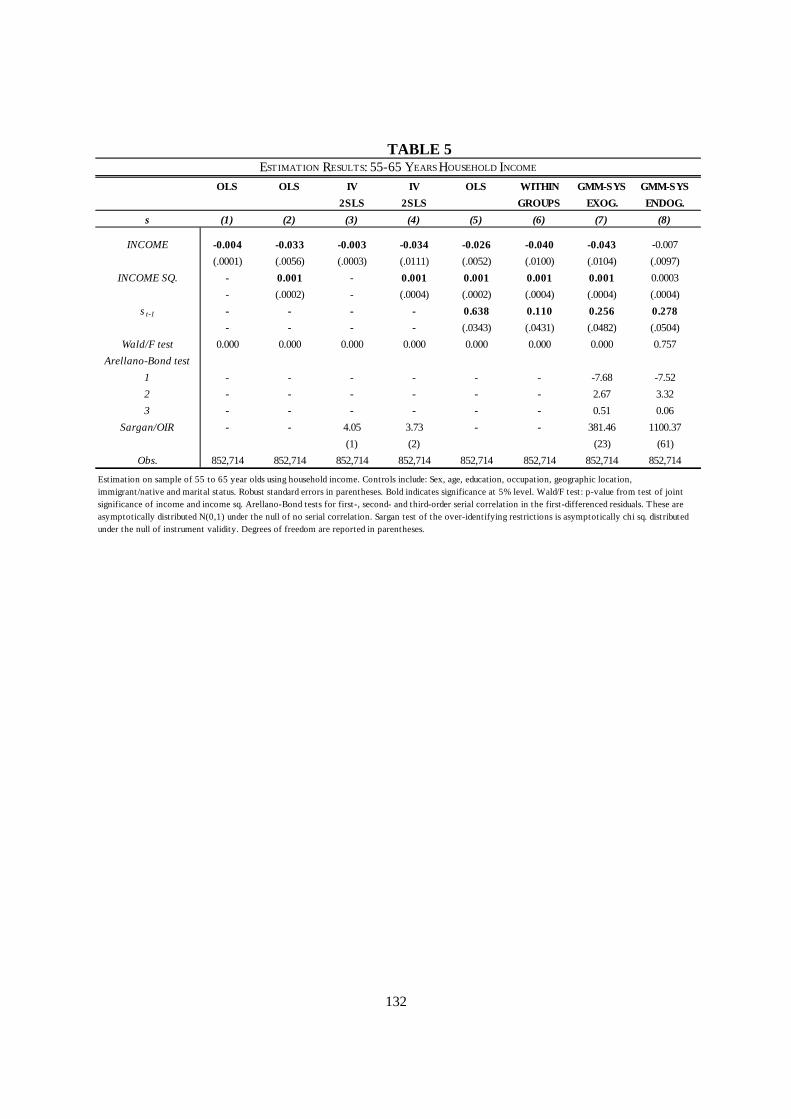
132
TABLE 5
OLS OLS IV IV OLS WITHIN GMM-SYS GMM-SYS
2SLS 2SLS GROUPS EXOG. ENDOG.
s (1) (2) (3) (4) (5) (6) (7) (8)
INCOME -0.004 -0.033 -0.003 -0.034 -0.026 -0.040 -0.043 -0.007
(.0001) (.0056) (.0003) (.0111) (.0052) (.0100) (.0104) (.0097)
INCOME SQ. - 0.001 - 0.001 0.001 0.001 0.001 0.0003
- (.0002) - (.0004) (.0002) (.0004) (.0004) (.0004)
s t-1 - - - - 0.638 0.110 0.256 0.278
- - - - (.0343) (.0431) (.0482) (.0504)
Wald/F test 0.000 0.000 0.000 0.000 0.000 0.000 0.000 0.757
Arellano-Bond test
1 - - - - - - -7.68 -7.52
2 - - - - - - 2.67 3.32
3 - - - - - - 0.51 0.06
Sargan/OIR - - 4.05 3.73 - - 381.46 1100.37
(1) (2) (23) (61)
Obs. 852,714 852,714 852,714 852,714 852,714 852,714 852,714 852,714
ESTIMATION RESULTS: 55-65 YEARS HOUSEHOLD INCOME
Estimation on sample of 55 to 65 year olds using household income. Controls include: Sex, age, education, occupation, geographic location, immigrant/native and marital status. Robust standard errors in parentheses. Bold indicates significance at 5% level. Wald/F test: p-value from test of joint significance of income and income sq. Arellano-Bond tests for first-, second- and third-order serial correlation in the first-differenced residuals. These are asymptotically distributed N(0,1) under the null of no serial correlat ion. Sargan test of the over-identifying restrict ions is asymptotically chi sq. distributed under the null of instrument validity. Degrees of freedom are reported in parentheses.

133
TABLE 6
OLS OLS IV IV OLS WITHIN GMM-SYS GMM-SYS
2SLS 2SLS GROUPS EXOG. ENDOG.
s (1) (2) (3) (4) (5) (6) (7) (8)
INCOME -0.016 -0.046 -0.015 -0.033 -0.028 -0.045 -0.051 -0.015
(.0004) (.0046) (.0010) (.0092) (.0036) (.0079) (.0084) (.0093)
INCOME SQ. - 0.001 - 0.001 0.001 0.001 0.001 0.0003
- (.0002) - (.0004) (.0002) (.0003) (.0003) (.0004)
s t-1 - - - - 0.620 0.124 0.256 0.301
- - - - (.0181) (.0242) (.0275) (.0311)
Wald/F test 0.000 0.000 0.000 0.000 0.000 0.000 0.000 0.000
Arellano-Bond test
1 - - - - - - -12.59 -12.80
2 - - - - - - 0.49 1.05
3 - - - - - - 0.14 0.42
Sargan/OIR - - 4.94 3.47 - - 80.32 250.49
(1) (2) (24) (62)
Obs. 427,814 427,814 427,814 427,814 427,814 427,814 427,814 427,814
ESTIMATION RESULTS: 55-65 YEARS - WOMEN
Estimation on sample of women, 55 to 65 year olds. Controls include: Age, education, occupation, geographic location, immigrant/native and marital status. Robust standard errors in parentheses. Bold indicates significance at 5% level. Wald/F test: p-value from test of joint significance of income and income sq. Arellano-Bond tests for first-, second- and third-order serial correlat ion in the first-differenced residuals. These are asymptotically distributed N(0,1) under the null of no serial correlat ion. Sargan test of the over-identifying restrict ions is asymptotically chi sq. distributed under the null of instrument validity. Degrees of freedom are reported in parentheses.

134
TABLE 7
OLS OLS IV IV OLS WITHIN GMM-SYS GMM-SYS
2SLS 2SLS GROUPS EXOG. ENDOG.
s (1) (2) (3) (4) (5) (6) (7) (8)
INCOME -0.006 -0.039 -0.005 -0.029 -0.032 -0.045 -0.050 -0.003
(.0002) (.0066) (.0005) (.0105) (.0060) (.0112) (.0121) (.0102)
INCOME SQ. - 0.001 - 0.001 0.001 0.002 0.002 0.0001
- (.0003) - (.0004) (.0002) (.0004) (.0005) (.0004)
s t-1 - - - - 0.589 0.074 0.225 0.256
- - - - (.0356) (.0432) (.0393) (.0426)
Wald/F test 0.000 0.000 0.000 0.000 0.000 0.000 0.000 0.455
Arellano-Bond test
1 - - - - - - -7.22 -7.04
2 - - - - - - 2.26 2.65
3 - - - - - - -1.04 -1.00
Sargan/OIR - - 0.78 0.01 - - 179.97 650.50
(1) (2) (24) (62)
Obs. 424,900 424,900 424,900 424,900 424,900 424,900 424,900 424,900
ESTIMATION RESULTS: 55-65 YEARS - MEN
Estimation on sample of men, 55 to 65 year olds. Controls include: Age, education, occupation, geographic location, immigrant/native and marital status. Robust standard errors in parentheses. Bold indicates significance at 5% level. Wald/F test: p-value from test of joint significance of income and income sq. Arellano-Bond tests for first-, second- and third-order serial correlat ion in the first-differenced residuals. These are asymptotically distributed N(0,1) under the null of no serial correlat ion. Sargan test of the over-identifying restrict ions is asymptotically chi sq. distributed under the null of instrument validity. Degrees of freedom are reported in parentheses.

135
Figures to be inserted in the text
FIGURE 1 KERNEL REGRESSION OF EXPENDITURE SHARE ON AGE
Local polynomial regression of age on the expenditure share. Cross-section, year 2003. Dashed lines are 95% confidence interval.

136
FIGURE 2 KERNEL REGRESSION OF LOG INCOME ON AGE
Local polynomial regression of age on the log income. Cross-section, year 2003. Dashed lines are 95% confidence interval.

137
FIGURE 3 KERNEL REGRESSION OF EXPENDITURE SHARE ON LOG INCOME
Local polynomial regression of log income on the prescription drug expenditure share. Cross-section, year 2003. Dashed lines are 95% confidence interval.

138
FIGURE 4 KERNEL REGRESSION OF EXPENDITURE SHARE ON LOG INCOME BY AGE GROUP
Local polynomial regression of log income on the prescription drug expenditure share by age. Young are individuals below the age of 55 and old are individuals aged 55 to 70. Cross-section, year 2003. Dashed lines are 95% confidence interval.

139
FIGURE 5 EXPENDITURE SHARE CHANGES FROM AGE 66 TO 68 FOR FULL SAMPLE
Plot of the predictions from the GMM-SYS estimator and the linear static model with income treated as endogenous. The dotted line is the actual expenditure share changes. The graph only depicts 80% of the distribution of income changes. 10% in the top/bottom has been left out. 95% confidence bands for GMM-SYS predictions are reported. These are bootstrapped using 1,000 replications.

140
FIGURE 6 EXPENDITURE SHARE CHANGES FROM AGE 66 TO 68 FOR SUB SAMPLE OF WAGE EARNERS AT 66
Plot of the predictions from the GMM-SYS estimator and the linear static model with income treated as endogenous. The dotted line is the actual expenditure share changes. The graph only depicts 80% of the distribution of income changes. 10% in the top/bottom has been left out. 95% confidence bands for GMM-SYS predictions are reported. These are bootstrapped using 1,000 replications.

SCHOOL OF ECONOMICS AND MANAGEMENT AARHUS UNIVERSITY – BARTHOLINS ALLÉ 10 – BUILDING 1322
DK-8000 AARHUS C – TEL. +45 8942 1111 - www.econ.au.dk
PhD Theses: 1999-4 Philipp J.H. Schröder, Aspects of Transition in Central and Eastern Europe. 1999-5 Robert Rene Dogonowski, Aspects of Classical and Contemporary European Fiscal
Policy Issues. 1999-6 Peter Raahauge, Dynamic Programming in Computational Economics. 1999-7 Torben Dall Schmidt, Social Insurance, Incentives and Economic Integration. 1999 Jørgen Vig Pedersen, An Asset-Based Explanation of Strategic Advantage. 1999 Bjarke Jensen, Five Essays on Contingent Claim Valuation. 1999 Ken Lamdahl Bechmann, Five Essays on Convertible Bonds and Capital Structure
Theory. 1999 Birgitte Holt Andersen, Structural Analysis of the Earth Observation Industry. 2000-1 Jakob Roland Munch, Economic Integration and Industrial Location in Unionized
Countries. 2000-2 Christian Møller Dahl, Essays on Nonlinear Econometric Time Series Modelling. 2000-3 Mette C. Deding, Aspects of Income Distributions in a Labour Market Perspective. 2000-4 Michael Jansson, Testing the Null Hypothesis of Cointegration. 2000-5 Svend Jespersen, Aspects of Economic Growth and the Distribution of Wealth. 2001-1 Michael Svarer, Application of Search Models. 2001-2 Morten Berg Jensen, Financial Models for Stocks, Interest Rates, and Options: Theory
and Estimation. 2001-3 Niels C. Beier, Propagation of Nominal Shocks in Open Economies. 2001-4 Mette Verner, Causes and Consequences of Interrruptions in the Labour Market. 2001-5 Tobias Nybo Rasmussen, Dynamic Computable General Equilibrium Models: Essays
on Environmental Regulation and Economic Growth.

2001-6 Søren Vester Sørensen, Three Essays on the Propagation of Monetary Shocks in Open Economies.
2001-7 Rasmus Højbjerg Jacobsen, Essays on Endogenous Policies under Labor Union
Influence and their Implications. 2001-8 Peter Ejler Storgaard, Price Rigidity in Closed and Open Economies: Causes and
Effects. 2001 Charlotte Strunk-Hansen, Studies in Financial Econometrics. 2002-1 Mette Rose Skaksen, Multinational Enterprises: Interactions with the Labor Market. 2002-2 Nikolaj Malchow-Møller, Dynamic Behaviour and Agricultural Households in
Nicaragua. 2002-3 Boriss Siliverstovs, Multicointegration, Nonlinearity, and Forecasting. 2002-4 Søren Tang Sørensen, Aspects of Sequential Auctions and Industrial Agglomeration. 2002-5 Peter Myhre Lildholdt, Essays on Seasonality, Long Memory, and Volatility. 2002-6 Sean Hove, Three Essays on Mobility and Income Distribution Dynamics. 2002 Hanne Kargaard Thomsen, The Learning organization from a management point of
view - Theoretical perspectives and empirical findings in four Danish service organizations.
2002 Johannes Liebach Lüneborg, Technology Acquisition, Structure, and Performance in
The Nordic Banking Industry. 2003-1 Carter Bloch, Aspects of Economic Policy in Emerging Markets. 2003-2 Morten Ørregaard Nielsen, Multivariate Fractional Integration and Cointegration. 2003 Michael Knie-Andersen, Customer Relationship Management in the Financial Sector. 2004-1 Lars Stentoft, Least Squares Monte-Carlo and GARCH Methods for American
Options. 2004-2 Brian Krogh Graversen, Employment Effects of Active Labour Market Programmes:
Do the Programmes Help Welfare Benefit Recipients to Find Jobs? 2004-3 Dmitri Koulikov, Long Memory Models for Volatility and High Frequency Financial
Data Econometrics. 2004-4 René Kirkegaard, Essays on Auction Theory.

2004-5 Christian Kjær, Essays on Bargaining and the Formation of Coalitions. 2005-1 Julia Chiriaeva, Credibility of Fixed Exchange Rate Arrangements. 2005-2 Morten Spange, Fiscal Stabilization Policies and Labour Market Rigidities. 2005-3 Bjarne Brendstrup, Essays on the Empirical Analysis of Auctions. 2005-4 Lars Skipper, Essays on Estimation of Causal Relationships in the Danish Labour
Market. 2005-5 Ott Toomet, Marginalisation and Discouragement: Regional Aspects and the Impact
of Benefits. 2005-6 Marianne Simonsen, Essays on Motherhood and Female Labour Supply. 2005 Hesham Morten Gabr, Strategic Groups: The Ghosts of Yesterday when it comes to
Understanding Firm Performance within Industries? 2005 Malene Shin-Jensen, Essays on Term Structure Models, Interest Rate Derivatives and
Credit Risk. 2006-1 Peter Sandholt Jensen, Essays on Growth Empirics and Economic Development. 2006-2 Allan Sørensen, Economic Integration, Ageing and Labour Market Outcomes 2006-3 Philipp Festerling, Essays on Competition Policy 2006-4 Carina Sponholtz, Essays on Empirical Corporate Finance 2006-5 Claus Thrane-Jensen, Capital Forms and the Entrepreneur – A contingency approach
on new venture creation 2006-6 Thomas Busch, Econometric Modeling of Volatility and Price Behavior in Asset and
Derivative Markets 2007-1 Jesper Bagger, Essays on Earnings Dynamics and Job Mobility 2007-2 Niels Stender, Essays on Marketing Engineering 2007-3 Mads Peter Pilkjær Harmsen, Three Essays in Behavioral and Experimental
Economics 2007-4 Juanna Schrøter Joensen, Determinants and Consequences of Human Capital
Investments 2007-5 Peter Tind Larsen, Essays on Capital Structure and Credit Risk

2008-1 Toke Lilhauge Hjortshøj, Essays on Empirical Corporate Finance – Managerial Incentives, Information Disclosure, and Bond Covenants
2008-2 Jie Zhu, Essays on Econometric Analysis of Price and Volatility Behavior in Asset
Markets 2008-3 David Glavind Skovmand, Libor Market Models - Theory and Applications 2008-4 Martin Seneca, Aspects of Household Heterogeneity in New Keynesian Economics 2008-5 Agne Lauzadyte, Active Labour Market Policies and Labour Market Transitions in
Denmark: an Analysis of Event History Data 2009-1 Christian Dahl Winther, Strategic timing of product introduction under heterogeneous
demand 2009-2 Martin Møller Andreasen, DSGE Models and Term Structure Models with
Macroeconomic Variables 2009-3 Frank Steen Nielsen, On the estimation of fractionally integrated processes 2009-4 Maria Knoth Humlum, Essays on Human Capital Accumulation and Educational
Choices 2009-5 Yu Wang, Economic Analysis of Open Source Software 2009-6 Benjamin W. Blunck, Creating and Appropriating Value from Mergers and
Acquisitions – A Merger Wave Perspective 2009-7 Rune Mølgaard, Essays on Dynamic Asset Allocation and Electricity Derivatives 2009-8 Jens Iversen, Financial Integration and Real Exchange Rates: Essays in International Macroeconomics 2009-9 Torben Sørensen, Essays on Human Capital and the Labour Market 2009-10 Jonas Staghøj, Essays on Unemployment and Active Labour Market Policies 2009-11 Rune Majlund Vejlin, Essays in Labor Economics 2009-12 Nisar Ahmad, Three Essays on Empirical Labour Economics 2010-1 Jesper Rosenberg Hansen, Essays on Application of Management Theory in Public
Organizations - Changes due to New Public Management 2010-2 Torben Beedholm Rasmussen, Essays on Dynamic Interest Rate Models and Tests for
Jumps in Asset Prices

2010-3 Anders Ryom Villadsen, Sources of Organizational Similarity and Divergence: Essays on Decision Making and Change in Danish Municipalities Using Organizational Institutionalism
2010-4 Eske Stig Hansen, Essays in Electricity Market Modeling 2010-5 Marías Halldór Gestsson, Essays on Macroeconomics and Economic Policy 2010-6 Niels Skipper, Essays on the Demand for Prescription Drugs