Aalto-D

D 87

/2016

9HSTFMG*aghjii+

ISBN 978-952-60-6798-8 (printed) ISBN 978-952-60-6799-5 (pdf) ISSN-L 1799-4934 ISSN 1799-4934 (printed) ISSN 1799-4942 (pdf) Aalto University School of Business Department of Economics www.aalto.fi

BUSINESS + ECONOMY ART + DESIGN + ARCHITECTURE SCIENCE + TECHNOLOGY CROSSOVER DOCTORAL DISSERTATIONS

Hanna V

irtanen E

ssays on Post-C

ompulsory E

ducation Attainm

ent in Finland

Aalto

Unive

rsity

2016

Department of Economics

Essays on Post-Compulsory Education Attainment in Finland

Hanna Virtanen

DOCTORAL DISSERTATIONS

978-951-628-661-0 (printed) 978-951-628-662-7 (pdf) 0356-7435 0356-7435 (printed)

E

linkeinoeläm

än tutkimuslaito

s, Sarja A

, Nro

49

Aalto University publication series DOCTORAL DISSERTATIONS

87 2016

Essays on Post-Compulsory Education Attainment in Finland

Hanna Virtanen

Aalto University School of Business Department of Economics

Elinkeinoelämän tutkimuslaitos, Sarja A, Nro 49

Main dissertation advisor Professor Pekka Ilmakunnas, Aalto University, Finland Co-dissertation advisors Professor Otto Toivanen, Katholieke Universiteit Leuven, Belgium Doctor Tuomas Pekkarinen, VATT Insititute for Economic Research Opponent Professor Edwin Leuven, University of Oslo, Norway

Aalto University publication series DOCTORAL DISSERTATIONS 87/2016 © Hanna Virtanen ISBN 978-952-60-6798-8 (printed) ISBN 978-952-60-6799-5 (pdf) ISSN-L 1799-4934 ISSN 1799-4934 (printed) ISSN 1799-4942 (pdf) http://urn.fi/URN:ISBN:978-952-60-6799-5 Unigrafia Oy Helsinki 2016 Finland

ISBN 978-951-628-661-ISBN 978-951-628-662-ISSN-L ISSN

Elinkeinoelämän tutkimuslaitos, Sarja A, Nro 49

0356-7435 (printed) 0356-7435

0 (printed) 7 (pdf)

Abstract Aalto University, P.O. Box 11000, FI-00076 Aalto www.aalto.fi

Author Hanna Virtanen Name of the doctoral dissertation Essays on Post-Compulsory Education Attainment in Finland Publisher School of Business Unit Department of Economics

Series Aalto University publication series DOCTORAL DISSERTATIONS 87/2016

Field of research Economics of Education

Date of the defence 3 June 2016

Monograph Article dissertation Essay dissertation

Abstract This thesis examines the determinants of upper secondary education attainment in Finland. The analyses build on register data for four cohorts of Finns leaving compulsory education in 2000–2003. The education outcomes are observed each year until 2012, and thus, the balanced observation period for all cohorts is nine years after the end of compulsory education. This gives the individuals abundant time to complete a degree, and those without a degree have often permanently dropped out from post-compulsory education. Essay 1 provides descriptive evidence for the determinants of the failure to complete any upper secondary education. The findings highlight the important role of prior achievement and parental background in predicting post-compulsory education attainment. The Essay also documents considerable variation in the association between the probability of graduating and regional availability of high school and vocational tracks. Furthermore, the results show that the initial upper secondary education choice after finishing compulsory education is very important for the overall completion probability. Essays 2 and 3 study how the centralized Finnish admission system impacts upper secondary enrolment and completion rates for applicants on the margin of receiving offers. I employ the regression discontinuity design created by the admission thresholds to estimate how admission to any upper secondary education position or to the first ranked application request affects the process of completing a post-compulsory degree. Each year, approximately 4 percent of the individuals leaving compulsory education and applying to upper secondary schools receive no offer in the application process. Essay 2 shows that rejection decreases the probability of completing a post-compulsory degree by approximately 7 to 9 percentage points. This equals to 10 to 15 percent of the potential graduation rate of the rejected applicants. Rejection also postpones graduation from upper secondary education substantially. Essay 3 explores how the discrepancy between an individual's aspirations and the study track in which he or she is admitted affects the process of completing an upper secondary degree. The results show that admission to an individual's first ranked education track increases the probability of graduating by approximately 4 percentage points

Keywords human capital, upper secondary education, dropping out, admission to education

ISBN (printed) 978-952-60-6798-8 ISBN (pdf) 978-952-60-6799-5

ISSN-L 1799-4934 ISSN (printed) 1799-4934 ISSN (pdf) 1799-4942

Location of publisher Helsinki Location of printing Helsinki Year 2016

Pages 127 urn http://urn.fi/URN:ISBN:978-952-60-6799-5

Tiivistelmä Aalto-yliopisto, PL 11000, 00076 Aalto www.aalto.fi

Tekijä Hanna Virtanen Väitöskirjan nimi Toisen asteen tutkinnon suorittaminen Suomessa Julkaisija Kauppakorkeakoulu Yksikkö Taloustieteen laitos

Sarja Aalto University publication series DOCTORAL DISSERTATIONS 87/2016

Tutkimusala Koulutuksen taloustiede

Väitöspäivä 03.06.2016

Monografia Artikkeliväitöskirja Esseeväitöskirja

Tiivistelmä Tämä väitöskirja muodostuu kolmesta toisiaan täydentävästä tutkimuksesta, joissa tarkastellaan toisen asteen tutkinnon suorittamiseen vaikuttavia tekijöitä. Analyysissä keskitytään siihen, miten erilaiset rajoitteet koulutuksen saatavuudessa vaikuttavat peruskoulun jälkeisen koulutuksen kysyntään ja suorittamiseen. Tutkimusaineisto perustuu pääosin Tilastokeskuksen rekisteriaineistoista ja se koostuu neljästä kohortista peruskoulun pättäviä opiskelijoita vuosilta 2000–2003. Aineistossa seurataan useiden vuosien ajan, aina vuoteen 2012 asti, näiden nuorten koulutukseen hakeutumista ja opinnoissa etenemistä. Essee 1 tuottaa kuvailevaa tietoa toisen asteen tutkinnon suorittamiseen vaikuttavista tekijöistä. Tulokset vahvistavat aikaisemman kirjallisuuden näkemystä siitä, että yksilöiden aikaisemmalla koulumenestyksellä sekä vanhempien taustaominaisuuksilla on tärkeä rooli peruskoulun jälkeisen tutkinnon suorittamiselle. Tutkimus löytää myös huomattavia eroja koulutuksen alueellisten tarjontarajoitteiden ja tutkinnon suorittamisen välisissä yhteyksissä riippuen siitä, minkä koulutusalan tarjonnassa rajoitteita esiintyy. Lisäksi tutkimuksessa todetaan, että välittömästi peruskoulun päättymisen jälkeen tehdyillä koulutuspäätöksillä on suuri merkitys yksilöiden valmistumiselle. Toisen asteen koulutuspaikat allokoidaan Suomessa keskitetyn yhteisvalinnan kautta. Väitöskirjan kaksi viimeistä esseetä hyödyntävät sisäänpääsyrajojen muodostamia epäjatkuvuuksia sisäänpääsytodennäköisyydessä. Regressioepäjatkuvuus lähestymistavan avulla tarkastellaan sitä, miten toisen asteen valinnassa menestyminen vaikuttaa opintojen etenemiseen. Noin neljä prosenttia niistä peruskoulusta valmistuvista yksilöistä, jotka osallistuvat toisen asteen yhteishakuun, jäävät kokonaan ilman koulutuspaikkaa. Essee 2 osoittaa, että koulutuksen ulkopuolelle jääminen heikentää yksilön todennäköisyyttä suorittaa peruskoulun jälkeinen tutkinto lähes 10 prosenttiyksikköä. Tämä vastaa noin 15 prosenttia ilman paikkaa jäävien suorittamistodennäköisyydestä. Koulutuksen ulkopuolellle jääminen aiheuttaa tämän lisäksi huomattavaa viivettä toisen asteen suorittamisen ajoittumiseen. Essee 3 näyttää, että myös sillä, tuleeko yksilö valituksi korkeimpaan vai alemmaksi sijoitettuun hakutoiveeseen on merkitystä koulutusprosessin onnistumiselle. Ensimmäiseen toiveeseen pääsy parantaa tutkinnon suorittamisentodennäköisyyttä noin neljällä prosenttiyksiköllä.

Avainsanat inhimillinen pääoma, toisen asteen koulutus, keskeyttäminen, opiskelijavalinta

ISBN (painettu) 978-952-60-6798-8 ISBN (pdf) 978-952-60-6799-5

ISSN-L 1799-4934 ISSN (painettu) 1799-4934 ISSN (pdf) 1799-4942

Julkaisupaikka Helsinki Painopaikka Helsinki Vuosi 2016

Sivumäärä 127 urn http://urn.fi/URN:ISBN:978-952-60-6799-5

ACKNOWLEDGEMENTS

My decision to enter the graduate program originated in the summer of 2002 when I worked as a research assistant in ETLA. The summer job turned into a responsi-bility for a research project, all thanks to Rita Asplund. I have learned a great deal about doing research from her, and Rita’s work served as an inspiration for me to pursue a career in research. It is also due to Rita’s influence that I have returned to ETLA. I am very pleased to be part of the community again and I extend my thanks to everybody there.

In ETLA I also became friends with Lotta Väänänen. She has played a crucial role in both, me making the decision to start the studies and succeeding to finish the project. Lotta’s incessant support and encouragement, as well as her direct input to my research have enabled the writing of this thesis. The moments working with her constitute the highlight of my studies. I value our friendship dearly.

My transition to the Department of Economics at the Aalto University School of Business (formerly known as Helsinki School of Economics) was very smooth, largely due to Pekka Ilmakunnas, my main supervisor and the head of the department at the time. I am very appreciative for my initial job as an assistant and for his kind aid in ensuring funding for the total duration of my studies. I thank Pekka for never giving up on me. I would like to express my gratitude to Otto Toivanen for generously taking me under his wings. His competence, extensive knowledge, and kindness have been inspirational. Otto’s influence will show in my work also beyond this thesis. I was very fortunate to have Tuomas Pekkarinen join my supervising team at the last years of my studies. I am grateful for his valuable comments and I am enthusiastic about our continued cooperation.

To have Edwin Leuven as a preliminary examiner and an opponent is a great honor. I have benefited a great deal from his insightful comments. I also thank Miik-ka Rokkanen for his useful comments that enable the improvement of my studies.

I owe my gratitude to numerous people who have contributed to this thesis. The project would not have been possible without the aid of the people at the Statistics Finland. Satu Nurmi was essential in putting the research data together. Vitally important was also the data I received from VATT with the contribution of Antti Moisio and Mika Kortelainen. Markku Hartonen from the National Board of Education has patiently answered the many questions I have had about the Finnish student admission process and data. Finally, I was fortunate to benefit from the editing skills of Kimmo Aaltonen. Thank you all, your efforts are greatly appreciated.

I gratefully acknowledge the financial support of the Finnish Doctoral Pro-gramme in Economics (FDPE) and the grants from Yrjö Jahnsson Foundation, OP Group Research Foundation, Finnish Cultural Foundation, HSE Foundation, and Palkansaajasäätiö. I am very thankful for the funding that enabled me to pursue my studies full-time.

The Department of Economics has provided a great atmosphere and facili-ties for learning and doing research. I would like to express my gratitude to Pertti Haaparanta and Juuso Välimäki who both served as heads of the department during my studies. Pertti, a fellow citizen of Lahti, made me feel at home there. He also guided the department through the transition to Aalto University and made it for us as painless as possible. I have utmost appreciation for the leadership of Juuso. I believe his influence shows in the inflow of very talented and ambitious people to the department during the last few years. My research has greatly benefited from the comments and discussions with the faculty members. Thank you especially to Manuel Bagues, Kristiina Huttunen, Matti Sarvimäki, Marko Terviö, and Natalia Zinovyeva.

It has also been a delight to work at the Helsinki Center of Economic Re-search (HECER) in the company of extremely bright people who share a passion for economics. I hope HECER is allowed to continue to flourish in the future. I also gratefully acknowledge the competent and helpful staff at the department and HECER. I thank Jutta Heino and Jenni Rytkönen also for bringing heaps of joy into my life.

I am grateful for Katja Ahoniemi, Olli Kauppi, Sami Napari, Hanna Pesola, and Satu Roponen who warmly welcomed me to the department and with whom I shared some memorable moments during the early years of my studies. I thank my fellow students Lassi Ahlvik, Kaisa Alavuotunki, Anni Heikkilä, Jenni Kello-kumpu, Eeva Kerola, Tero Kuusi, Milla Nyyssölä, Tuuli Paukkeri, Anna Sahari, Tanja Saxell, Nelli Valmari, and Suvi Vasama. You made this project bearable even when I struggled with my work. I am glad we had the chance to connect also on a non-professional level. I have been fortunate to share the same office space with several inspirational people. I thank Chang-Koo Chi, Rob Gillanders, and Christian Krestel for easing the pressure to finish this thesis via their support and humor.

The advantage of taking a long time to graduate is that I have had a chance to meet numerous colleagues and many generations of PhD students. In fact, it is impossible for me to make a comprehensive list of all the wonderful people who have influenced my studies. It has been an unforgettable experience thanks to all of you.

A part of this research was carried out while visiting the Centre for Economic Performance (CEP) at London School of Economics (LSE). I thank Stephen Machin and Sandra McNally for facilitating the visit, and all the colleagues for making the experience enjoyable. I am especially grateful for the fellow students at CEP who helped me during some turbulent times.

Nothing in my life, including this thesis, would be possible if it were not for my friends and family. I would especially like to thank Katja and Ari. On many occasions it was only with your support that I could carry on. Equally important have been the numerous times you ridiculed me and helped me see the absurdities of my chosen profession. I am also very grateful for my other amazing friends who enrichen my life and make me complete. The help I have received in taking care of my daughter has been priceless.

I am in deep gratitude to my mother Riitta, who has been my sheet anchor throughout the years. I thank you mom for all that you have done for me, for your endless love and solicitude for me. It makes all the difference.

My daughter Heta deserves special thanks. She has been my biggest moti-vation for completing this thesis, as well as the greatest hurdle I had to overcome to finish the work. I believe there is also no better stress reliever than a bubbly toddler. I love you sweetie.

I would like to dedicate this thesis to Arto Saranjoki. He was a pivotal factor that approximately 20 years ago made me choose Economics, instead of Social Policy like I had planned. He argued that studying economics would allow me to explore the same topics. However, if I ever attempted to have an impact on the related policies, I would have remarkably better odds doing that when participating in the conversation as an economist. I hope he was right.

Contents

AcknowledgementsIntroduction 9References 14

Essay 1 Determinants of dropping out of post-compulsory education in Finland 17 1. Introduction 18 2. Theoretical framework 21 3. Institutional background 22 4. Data and variables 23 4.1. Data sources 23 4.2. Educational attainment 23 4.3. Sample and individual background characteristics 24 4.4. Availability of education 25 4.5. Choice of what and where to study 27 5. Econometric model 27 6. Determinants of educational attainment 29 6.1. Individual background characteristics 29 6.2. Availability of education 32 6.3. Field of education 35 7. Discussion 36 References 37 Figure 40 Tables 41 Appendices 49

Essay 2 Failure in admission and the process of completing a post-compulsory degree 57 1. Introduction 58 2. Institutional background and data 60 2.1. Joint application system 60 2.2. Data and analysis sample 62 3. Empirical strategy 63 3.1. Determining the threshold 63 3.2. Assignment variable 64 3.3. Empirical specification 65 3.4. Identification strategy 66

4. Results 68 4.1. Probability of completing upper secondary degree 68 4.2. Process of completing upper secondary degree 69 4.3. Heterogeneous effects 70 4.4. Robustness checks 71 5. Discussion 72 References 73 Figures 75 Tables 79 Appendix 1 83

Essay 3The effect of admission to a more preferred education track on the probability of completing post-compulsory education 89 1. Introduction 90 2. Application to upper secondary education 93 3. Data 94 3.1. Data sources 94 3.2. Analysis sample 95 4. Empirical strategy 96 4.1. Assignment variable 96 4.2. The empirical specification 97 4.3. Identification strategy 98 5. Results 100 5.1. Main effects 100 5.2. Heterogeneous effects 102 5.3. Robustness checks 104 6. Discussion 105 References 108 Figures 110 Tables 114

ESSAYS ON POST-COMPULSORY EDUCATION ATTAINMENT IN FINLAND

This dissertation consists of an introduction and the following single-authored three essays.

Essay 1:“Determinants of dropping out of post-compulsory education in Finland”, un-published.

Essay 2:“Failure in admission and the process of completing a post-compulsory degree”, unpublished.

Essay 3:“The effect of admission to a more preferred education track on the probability of completing post-compulsory education”, unpublished.

9

Introduction

INTRODUCTION

Social exclusion of youth is considered one of the most important challenges of the current Finnish economy. The president of Finland, Sauli Niinistö, has become a recognized patron of the issue. In 2012, President Niinistö launched a campaign that aimed to inform the public about the social exclusion of youth1. There has also been a boom of reports and studies attempting to tackle the problem (e.g., Alatupa et al., 2007; Myrskylä, 2012; Tuomala, 2013; Aaltonen et al., 2015), and the topic has received extensive media coverage.

Concerns have been raised over the wasted labor force in an aging society, the costs of health care and social welfare, and the human tragedy for those con-cerned, for example. Rough estimates of the total costs of an individual socially excluded from society vary between €1 million and €1.8 million (e.g., Alatupa et al., 2007; Leinonen, 2012; Myrskylä 2012). Although these estimates may not survive scientific scrutiny, it is clear that the related costs are substantial. Social exclusion is often a persistent phenomenon in which several problems accumulate one after another. A recent research report by the National Institute for Health and Welfare and the Finnish Youth Research Society estimated that the annual health care costs of socially excluded youth alone are five to seven times as high as those of young individuals with no signs of social exclusion (Aaltonen et al., 2015).

Upper secondary education has great importance in preventing social exclu-sion. First, an upper secondary degree is in itself part of the most commonly used definition, where a socially excluded individual is defined as someone who has no post-compulsory degree and is outside the labor force and education. Furthermore, there appears to be broad consensus that education, an upper secondary degree in particular, is the most powerful tool for enhancing labor market participation. According to my research data on individuals leaving compulsory education during the years 2000–2003, those with no post-compulsory degree 10 years later have a 40 percent employment rate, whereas the corresponding figure for those with at least an upper secondary degree varies between 70 and 90 percent depending on the field and level of their education. Furthermore, the probability of being entirely outside the labor force and education is four times higher for those without any upper secondary degree than that observed for their counterparts with a post-compulsory degree.

In Finland, about 15 percent of each age group who is 25 years or older have no upper secondary degree (Labour Force Survey, 2014). This totals almost 10,000 individuals per cohort who leave compulsory education. More information is needed on how to prevent individuals from dropping out from post-compul-sory education. This thesis provides empirical evidence for the determinants of post-compulsory educational attainment. The focus is on supply-side institutions that may be affected by policy measures.

1 Press release of the Office of the President of the Republic of Finland. 12.6.2012. “Tasavallan presidentti kokoaa arkikeinoja syrjäytymisen ehkäisyyn”. http://www.tpk.fi/public/default.aspx?contentid=251197&nodeid=46542&contentlan=1&culture=fi-FI. Referenced in 3.6.2015.

10

Introduction

My thesis consists of three studies that examined upper secondary education choices and their link to various supply constraints. For this purpose, I constructed a very rich dataset of four cohorts of Finns graduating from compulsory education in 2000–2003. I have information on their application, admission, enrollment, and completed degrees up to 2012. In addition to the information on education choices and outcomes, I also have detailed information on the characteristics of the individuals, their family background, and their residential regions. I worked on this unique dataset using state-of-the-art research methods.

Essay 1 explores the determinants of failure to complete any upper secondary education with a focus on the regional supply constraints and the choice of educa-tion field. To my knowledge, this paper is one of the few studies that has examined the link between the regional supply of education and upper secondary education choices (Dickerson and McIntosh, 2013; Falch et al., 2013), and the first to con-sider how proximity to the education track in which an individual is enrolled is associated with the decision to drop out. The results for the link between regional supply and the probability of completing an upper secondary degree are mixed. The availability of upper secondary educational institutions in the municipality of residence is found to have a large, 8-10 percentage point positive association with the probability of graduating for boys and for those with low prior achievement. However, the association is evenly large and negative for girls and for those with a prior school performance that was a little above the median. More detailed analysis provides evidence that the availability of high school and the vocational field of humanities and teaching have a negative influence on the decision to drop out for the individuals with below median prior achievement, whereas the supply of the fields of administration and commerce and social and health care services have a positive correlation with the educational attainment of this sub-group. Further-more, the availability of the field of culture has a negative association with the probability of graduating for boys and a positive association with the probability of graduating for girls.

Regional supply constraints are likely to also play a role in determining the distance from home to the location where an individual is enrolled. According to the findings in Essay 1, being enrolled in a school in a municipality other than the individual’s municipality of residence at the end of compulsory schooling has an approximately 2 percentage point negative influence on the probability of com-pleting a post-compulsory degree when compared to those enrolled in their initial municipality of residence for all sub-groups except for those with the highest prior achievement. Individuals with high prior school performance have a consistently high completion rate, and their probability of graduating appears to be insensitive to almost everything.

Finally, Essay 1 contributes to the growing literature on the differences across education fields (e.g., Arcidiacono, 2004; Malamud and Pop-Eleches, 2010; Reyes et al., 2013; Hastings et al., 2013; Kirkebøen et al., 2014). The results show that the initial upper secondary education choice directly after the end of compulsory education is very important for the overall probability of completing a post-com-

11

Introduction

pulsory degree. As expected, not being enrolled in school in the first autumn after the end of compulsory education is negatively associated with the probability of graduating. Furthermore, the findings show that those with a below median grade point average (GPA) are more likely to complete a post-compulsory degree if they have chosen vocational education instead of high school. The opposite is true for individuals with an above median GPA in the comprehensive school leaving certif-icate. As we show in another study (Virtanen and Väänänen, 2015), the percentage of individuals with low prior school performance who apply to high school as their first choice or choosing the outside option of not applying to upper secondary ed-ucation would have been reduced by 5 to 10 percent by improving the availability of vocational fields. Thus, at least part of the influence of the education field choice on the dropout rate may be driven by regional supply constraints.

Each year, around 6 percent of the individuals who leave compulsory ed-ucation and apply to upper secondary schools fail to enroll in post-compulsory education in Finland. In Essays 2 and 3, I examine how success in the admission process contributes to this problem. Admission to upper secondary schools takes place through the centralized application system maintained by the Finnish National Board of Education. Individuals can simultaneously apply to five differ-ent schooling positions where a schooling position is defined as an educational institution–track combination. Individuals are allocated to the predetermined number of open positions based on admission points. As there are generally more applicants than schooling positions, for each educational institution–track entry, there is a threshold level above which individuals can enter the schooling position. Individuals are offered the highest ranked schooling position for which their admission points are above the threshold level. Those below the thresholds of all of their requests are not offered any schooling position.

In Essays 2 and 3, I employ the regression discontinuity design (RDD) created by the admission thresholds to estimate how admission to any upper secondary education position or to the first ranked application request affects the process of completing a post-compulsory degree. The idea in the RD design is to exploit the “randomness” of the allocation of people in the close neighborhood of the threshold and compare individuals just below and above the threshold (for a more detailed description of the method, see Imbens and Lemieux, 2008; Lee and Lemieux, 2010). This allows me to estimate the causal effect of the treatment at the threshold (the local average treatment effect). Similar admission thresholds are used to study the effect of attending high-achieving educational institutions (e.g., Hoekstra, 2009; Saavedra, 2009; Pop- Eleches and Urquiola, 2011) and returns to education fields (e.g., Hastings et al., 2013; Kirkebøen et al., 2014).

In Essay 2, I examine whether education outcomes differ for those who are barely able to secure any schooling position compared to those who are among the first ones left without any schooling position. The number of open positions avail-able in upper secondary schools is larger than the size of the cohort that graduates from compulsory schools each year (approximately 1.5 positions per individual). However, individuals from previous cohorts also apply to upper secondary schools

12

Introduction

(those who have taken a break in their studies after compulsory education or who want to switch their education choice) and thus crowd the application process. Furthermore, there are large regional disparities in the upper secondary supply that may create a mismatch between the location of the applicants and available schooling positions. In addition, the applicants’ preferences may not match the distribution of available positions across the education alternatives in the region. As a result, approximately 4 percent of applicants who just graduated from compulsory education are left outside upper secondary education in the application process.

The findings show that rejection decreases the probability of ever enrolling in upper secondary schools and increases the probability of dropping out conditional on enrollment, leading to a lower overall probability of completing a post-com-pulsory degree. Furthermore, failure to gain admission also postpones graduation from upper secondary education substantially. The probability of completing an upper secondary degree is decreased by approximately 7 to 9 percentage points. This is equal to 10 to 15 percent of the potential graduation rate of the rejected applicants in the case of admission. The rejected applicants are typically students with low prior achievement and from more challenging backgrounds, and thus, the repercussion of their early school leaving may be very serious.

Furthermore, the results in Essay 2 show that receiving no offer in the ad-mission process affects the educational attainment of individuals who live in small cities and rural Finland significantly more than of those who live in the 15 largest cities. The estimated impact on the probability of completing a post-compulsory degree in 9 years is 14 percentage points in small cities, whereas the corresponding figure for individuals who live in large cities is less than 3 percentage points and is statistically insignificant. Although smaller cities perform better in terms of the overall completion rate, the results of this study suggest that the reallocation pro-cess of vacant schooling positions may be more efficient or that there may be more rigorous alternatives for a gap-year activity in large cities. These findings emphasize the need for improved (geographic) matching of the demand and supply of upper secondary education and that more efficient policies for those left outside all up-per secondary education positions are important in facilitating high-risk groups.

Essay 3 explores how the discrepancy between an individual’s aspirations and the study track to which he or she is admitted affects the process of completing a post-compulsory degree. If individuals have strong preferences for education alternatives, then getting into a preferred education track may be crucial to these individuals’ performance. Identifying the causal effect of admission success on education outcomes can be challenging. First, those admitted to their highest ranked request, on average, are individuals with better prior school performance than those rejected by their first request. On the other hand, the highest-ranked education tracks may be more selective institutions, and thus, the better observed performance of those admitted to their highest request may be due to the difference in the quality of the educational institutions. This study overcomes these difficulties by utilizing an admission mechanism that effectively randomizes applicants near the unpredictable admission threshold into education tracks. This, together with

13

Introduction

the upper secondary education system, in which individuals choose between several unordered education alternatives, allows me to separate the causal effect of admis-sion to a preferred education track from the effect of admission to any given track.

The results show that admission to the first ranked education track increas-es the probability of completing a post-compulsory degree by approximately 4 percentage points. Furthermore, the results provide evidence that the initial participation decision and the choice to switch education tracks are sensitive to admission success, whereas the overall probability of ever enrolling appears to be unaffected by admission to the highest request. In addition, admission to the first request track has an impact on the dropout decision, but only for some subgroups of applicants. Admission to a more preferred track affects mainly the education process of those with lower levels of prior educational achievement. According to the estimates, the probability of graduating could be increased by more than 10 percentage points, if they are admitted to their first request. This is equal to more than 15 percent of the overall probability of this group to complete an upper sec-ondary degree. Although this study provides no evidence that admission to the first request affects the probability of graduating for high achievers, it does not mean that there are no consequences for matching high achievers to a lower ranked education track. Admission success can still affect their labor market outcomes as shown in Kirkebøen et al. (2014).

The results in Essay 3 indicate that interruptions in the education process caused by the failure to gain admission to the highest-ranked request lead to a decreased probability of graduating. Therefore, it could be beneficial to have an educational system that enables students to flexibly revise their initial track choices at later stages of their studies as suggested by Dustmann et al. (2012). In addition, based on the results in Goux et al. (2014), improving student counseling could be an effective method for enhancing the assignment of individuals to the upper secondary tracks. They find that increasing information about low-achieving pupils and their parents about upper secondary degree alternatives and pupils’ abilities affects the upper secondary education choice and increases participation in post-compulsory education. Individuals who receive additional student coun-seling apply more often to less ambitious vocational tracks instead of to the most selective high school tracks. This is followed by increased success in receiving an offer to the demanded track and a reduction in the dropout rate. More information may be important to help individuals make more realistic application choices that protect them from needless disappointment.

The findings in this thesis suggest that individuals’ preferences should not be ignored when planning the supply of education tracks. Finland is a sparsely inhabited and geographically large country. Thus, there is pressure to increase the efficiency of the supply of education by concentrating on educational institutions into larger units in large municipalities. Based on the results, increasing the re-gional disparity in supply can have disadvantageous effects on post-compulsory educational attainment, particularly for individuals with low prior achievement and a high risk of early school leaving.

14

Introduction

REFERENCESAaltonen, S., Berg, P., and Ikäheimo, S. (2015) “Nuoret luukulla. Kolme näkökul-

maa syrjäytymiseen ja nuorten asemaan palvelujärjestelmässä”, a report from Finnish Youth Research Society and National Institute for Health and Welfare.

Alatupa, S. (editor), Karppinen, K., Keltikangas-Järvinen, L., and Savioja, H. (2007) “Koulu, syrjäytyminen ja sosiaalinen pääoma- Löytyykö huono-osaisuuden syy koulusta vai oppilaasta?”, Sitra report 75.

Arcidiacono, P. (2004) “Ability sorting and the return to college major”, Journal of Econometrics, 121, 343-375.

Card, D. (2001) “Estimating the return to schooling: progress on some persistent econometric problems”, Econometrica, 69:5, 1127-1160.

Dickerson, A. and McIntosh, S. (2013) “The impact of distance to nearest education institution on the post-compulsory education participation decision”, Urban Studies, 50:4, 742-758.

Dustmann, C., Puhani, P., and Schönberg, U. (2012) “The long-term effects of school quality on labour market outcomes and educational attainment”, Centre for Research and Analysis of Migration (CReAM) Discussion Paper Series 1208.

Falch, T., Lujala, P., and Strøm, B. (2013) “Geographical constraints and educational attainment”, Regional Science and Urban Economics, 43, 164-176.

Goux, D., Gurgand, M., and Maurin, E. (2014) “Adjusting your dreams? The effect of school and peers on dropout behaviour”, IZA Discussion Paper No. 7948.

Hastings, J., Neilson, C., and Zimmerman, S. (2013) “Are some degrees worth more than others? Evidence from college admission cutoffs in Chile”, NBER Working Paper No. 19241.

Hoekstra, M. (2009) “The effect of attending the flagship state university on earn-ings: A discontinuity based approach”, Review of Economics and Statistics, 91:4, 717-724.

Imbens, G.W. and Lemieux, T. (2008) “Regression discontinuity designs: a guide to practice”, Journal of Econometrics, 142, 615-635.

Kirkebøen, L., Leuven, E., and Mogstad, M. (2014) “Field of study, earnings, and self-selection”, NBER Working Paper 20816.

Lee, D. and Lemieux, T. (2010) “Regression discontinuity design in economics”, Journal of Economic Literature, 48, 281-355.

Leinonen, T. (2012) “Nuorten koulutuksen keskeyttäminen ja sen hinta”, Sosiaa-likehitys Oy, Opit käyttöön hanke.

Malamud, O. and Pop-Eleches, C. (2010) “General education versus vocational training: evidence from an economy in transition”, The Review of Economics and Statistics, 92:1, 43-60.

Myrskylä, P. (2012) “Hukassa – Keitä ovat syrjäytyneet nuoret?”, EVA Analyysi 19/2012, Helsinki: Elinkeinoelämän valtuuskunta.

Pop-Eleches, C. and M. Urquiola (2013) “Going to a better school: effects and behavioral responses”, American Economic Review, 103:4, 1289-1324.

15

Introduction

Reyes, L., Rodrigues, J., and Urzula, S. (2013) “Heterogeneous economic returns to postsecondary degrees: evidence from Chile”, NBER Working Paper No. 18817.

Saavedra, J. (2009) “The learning and early labor market effects of college quality: A regression discontinuity analysis”, Mimeo, Harvard University.

Tuomala, E. (2013) “Social Exclusion of Young People in Finland”, Bachelor in Business Administration Double Degree European Management Thesis, Helsinki Metropolia University of Applied Sciences, 4.10.2013.

Virtanen, H. and Väänänen, L. (2015) “Regional supply and student sorting”, unpublished manuscript.

17

Essay 1

ESSAY 1

DETERMINANTS OF DROPPING OUT OF POST-COMPULSORY EDUCATION IN FINLAND

Abstract

This paper explores the determinants of the failure to complete an upper second-ary degree. The findings highlight the important role of prior achievement and parental background in predicting post-compulsory educational attainment. The chapter also documents considerable variation in the association between the probability of graduating and regional availability of high school and vocational tracks. Furthermore, the results show that the initial upper secondary education choice immediately after finishing compulsory school is very important for the overall probability of completing an upper secondary degree. Enrollment in upper secondary education in another municipality and not being enrolled in school are associated with a lower probability of graduating. The findings also show that those with below median grade point averages (GPAs) are more likely to complete post-compulsory education if they have chosen vocational education instead of high school. The opposite is true for individuals with above median GPAs.

18

Essay 1

1. INTRODUCTIONDecreasing upper secondary education dropout rates stands high on the priority list of education policy in most Organization for Economic Cooperation and De-velopment (OECD) countries. The percentage of Finns age 20 to 24 years old with only a lower secondary degree (comprehensive schooling) is close to 15 percent, which is only slightly better than the EU28 average of 17-18 percent (Labour Force Survey, 2014). Failure to complete upper secondary education is a serious concern as it is often considered the minimum requirement for successful labor market entry and can have adverse consequences for health outcomes, criminal behavior, and social exclusion (see e.g. Lochner, 2011; Grossman, 2006). Thus, understanding the determinants of dropping out is crucial, particularly for factors that can be affected by policy tools. This paper explores the determinants of failure to complete any upper secondary education with a focus on the regional supply constraints and the choice of the field of education. Although focused on Finland, this paper informs similar debates on early school leaving in many European countries and in the United States (US) as well1.

Many of the previous studies on the determinants of post-compulsory edu-cation attainment examined the participation decision during the first few years after the end of compulsory education (e.g., Maani and Kalb, 2007; Bradley and Lenton, 2009; Casquel and Uriel, 2009; Dickerson and MacIntosh, 2013) or the probability of completing an upper secondary degree within the three-year target duration (Falch et al., 2013). However, the school paths to a degree are diverse, and young people may switch between being enrolled and being outside of education several times (see Albaek et al., 2015, for the Nordic case). Therefore, the enroll-ment status at any given point in time is not enough to distinguish between those who actually fail to complete a post-compulsory degree and those who are merely taking a break in their studies. Furthermore, although decreasing the duration of upper secondary education studies may also be important and is a constant concern for policy makers, the failure to complete an upper secondary degree has more dramatic consequences for the individual and society.

This study uses a very rich dataset on four cohorts of Finns leaving compul-sory education in 2000–2003. The education outcomes are observed each year until 2012, and thus, the balanced observation period for all cohorts is nine years after the end of compulsory education (until the age of 25). This gives the individuals abundant time to complete a degree, and those without a degree have often per-manently dropped out from post-compulsory education. Moreover, the data has detailed information on prior achievement, other individual characteristics, and family background, as well as on regional characteristics. This enables me to take

1 In the US, concern focuses on high school dropout rates. In the US, high school graduation occurs at age 18, and in Finland, as in most other countries in Europe, upper secondary education takes place between the ages 16 and 19 (in some European countries, the upper secondary curriculum is 2 years, and the target gradu-ation is then accordingly age 18).

19

Essay 1

into account an extensive list of factors shown in previous research to be import-ant for educational attainment (for extensive summaries, see Rumberger and Lim (2008) and Lyche (2010)).

In line with previous research, I find that prior achievement is a strong predictor of post-compulsory education attainment. A one standard deviation increase in the GPA of theoretical subjects is associated with a 10 percentage point improvement in the probability of completing an upper secondary degree. The results also show that grades for sports education and arts and craft have additional influence on propensity to drop out. Furthermore, this study provides evidence that written and verbal skills are more important for upper secondary graduation than math skills. Those who graduate at age 17 from compulsory education, a year later than the standard age for graduation, have a more than 10 percentage point lower probability of completing an upper secondary degree than those who leave compulsory education at age 15 or 16. Taking all this evidence together, it appears that prior school success is a very important determinant of post-compulsory education attainment.

This study also shows that parental background influences the propensity to drop out from upper secondary education. As expected based on previous studies, those with more educated parents and higher family income are more likely to complete a post-compulsory degree. The graduation probabilities for boys and girls are more sensitive to the maternal education level than to the paternal education level when prior school performance is controlled for.

The analysis concentrates on how the local availability of upper secondary education alternatives influences the propensity to drop out. The institutional setting in Finland provides a good opportunity to explore the influence of regional constraints. Finland is a geographically large country with a small population, and thus, there are large disparities in the regional supply. At the same time, the supply of upper secondary education is closely monitored by the Ministry of Education, and the institution network is homogeneous. To my knowledge, this paper is one of the few studies that has examined the link between the regional education supply and upper secondary education choices (Dickerson and McIntosh, 2013; Falch et al., 2013), and the first to consider how proximity to the education track in which an individual is enrolled is associated with the decision to drop out.

The results for the link between the regional supply and the probability of completing an upper secondary degree are mixed. The availability of an upper secondary school in the municipality of residence is found to have a large, 8-10 percentage point positive association with the probability of graduating for boys and for those with low prior achievement. However, the association is equally large and negative for girls and for those with a prior school performance a higher than the median. More detailed analysis provides evidence that the availability of high school and the vocational field of humanities and teaching has a negative influence on the propensity to drop out for individuals with below median prior achievement, whereas the supply of the fields of administration and commerce and social and health care services has a positive correlation with the educational

20

Essay 1

attainment of this sub-group. The availability of the field of culture has a negative association with the probability of graduating for boys and a positive association with the probability of graduating for girls.

Regional supply constraints are likely to play a role in determining the dis-tance from home to the location where an individual is enrolled. Being enrolled in a different municipality than the individual’s municipality of residence at the end of compulsory school has an approximately 2 percentage point negative in-fluence on the probability of completing a post-compulsory degree compared to those enrolled in their initial municipality of residence for all sub-groups except for those with the highest prior achievement. Individuals with high prior school performance have consistently high completion rates, and their probability of graduating appears to be insensitive to almost everything.

Finally, this study contributes to the growing literature on the differences across education fields (e.g., Arcidiacono, 2004; Malamud and Pop-Eleches, 2010; Reyes et al., 2013; Hastings et al., 2013; Kirkebøen et al., 2014). This interest has been triggered by the observation that there are larger differences in returns across education fields than there are across education institutions. In this study, I provide descriptive evidence for the influence of the chosen education field on the probability of dropping out from post-compulsory education while controlling for an extensive set of background variables.

The results show that the initial upper secondary school choice directly after the end of compulsory education is very important for the overall completion probability. As expected, being outside of education the first autumn is negatively associated with the probability of graduating. Furthermore, the findings show that those with a below median GPA are more likely to complete a post-compulsory degree if they have chosen vocational education instead of high school. The opposite is true for the individuals with an above median GPA. In another study (Virtanen and Väänänen, 2015), we show that the percentage of individuals with low prior school performance who apply to high school as their first request or choose the option of not applying to an upper secondary school would have been reduced by close to 10 percent by improving the availability of vocational fields. Thus, at least part of the influence of the education field choice on the dropout rate may be driven by regional supply constraints.

The rest of the chapter is organized as follows. In the next section, I briefly discuss the standard theoretical framework used to study the determinant of dropping out of post-compulsory education. In section 3, I describe the education system in Finland. In section 4, I define the data in detail and present descriptive statistics. In sections 5 and 6, I present the empirical model and the results, and I conclude in section 7.

21

Essay 1

2. THEORETICAL FRAMEWORKHuman capital theory as put forward by Mincer (1958) and Becker (1962: 64) provides the standard theoretical framework for studying education choices. Ac-cording to the model, an individual invests in education if the present discounted value of the benefits from doing so is greater than or equal to the costs. Benefits are typically measured by an increase in lifetime earnings whereas costs are considered to include opportunity costs as well as the direct costs of tuition, materials, and transportation. More recent developments in the theory suggest that individuals are faced with uncertainty when they make school decisions (Manski, 1989; Altonji, 1993). Individuals have uncertainty about the feasibility and desirability of com-pleting a degree in general, as well as about which schooling alternative gives them the highest utility. Under uncertainty, individuals make their schooling choices sequentially each period with updated information. Learning about one’s abilities and about the match value may lead a young person to drop out.

There is a large amount of literature on the determinants of dropping out. Much of the previous work examine the importance of individual and family characteristics on the decision to drop out (e.g., Bradley and Lenton, 2007; Belly and Lochner, 2007; Maani and Kalb, 2007; Casquel and Uriel, 2009). Individuals differ in their net benefits from schooling, preferences, and in the risk of failure that leads to different optimal education decisions for different individuals (Willis and Rosen, 1979; Eckstein and Wolpin, 1999). Furthermore, some young people may be better in forming their expectations, and thus, the propensity to drop out may vary with individual and family characteristics (Bradley and Lenton, 2007).

Some of the previous work focuses on the impact of peer and school char-acteristics on educational attainment (e.g., Lee and Barro, 2001; Bobonis and Finan, 2009; Maliranta et al., 2010). A typical framework used in these studies is to consider school-related factors as inputs in the education production process (see Hanushek, 1986; Sacerdote, 2011). In related literature, some authors examine the importance of local labor market conditions on post-compulsory schooling decisions (e.g., Rice, 2010; Meschi et al., 2011). The situation in the labor market can affect the expected returns for education, as well as the opportunity costs of investing in education (see Micklewright et al., 1990).

Another strand of literature considers how geographic proximity affects education decisions. Distance to schooling can cause direct financial costs of re-allocation or commuting, emotional costs associated with leaving home, and information costs when seeking information about school options (see Dickerson and McIntosh, 2013). Only a few papers have examined the effects of regional availability in the context of the upper secondary education decision (Dickerson and McIntosh, 2013; Falch et al., 2013).

Finally, there is growing literature that examines the effects of policies aimed at preventing students from dropping out (e.g., Dearden et al., 2009; Felgueroso et al., 2014; Goux et al., 2015). The decision to drop out may reflect an accurate eval-uation of the net benefits of remaining in education. However, the social returns of

22

Essay 1

education are commonly assumed to exceed the private returns making it attractive from society’s point of view to provide incentives for individuals to continue their education. Furthermore, Oreopoulus (2007) suggests that many adolescents heav-ily discount or simply ignore the future consequences of dropping out, implying that dropping out may be suboptimal even for the individual making the choice.

3. INSTITUTIONAL BACKGROUNDCompulsory education in Finland consists of nine years of comprehensive school-ing, and it typically begins at age seven. A person’s legal responsibility to participate in compulsory education ends with completion of comprehensive schooling or 10 years after the initial enrollment. The completion rate in Finland is very high: 99.7 percent of Finnish children graduate from comprehensive schooling (Finnish National Board of Education).

After graduating from compulsory education, one can continue to upper secondary education, continue for an additional year in comprehensive schooling (10th grade), or decide not to study further. A voluntary additional year in compre-hensive schooling prepares individuals for upper secondary education and provides an opportunity to improve grades. Upper secondary education is divided into high school and vocational education. High school has general tracks (academic study programs) and tracks that have specific orientation to subjects such as music or sports (specialized study programs). High school ends with the national matricu-lation examination. Vocational education and training include seven fields: natural resources, technology and transport, administration and commerce, hotel, catering, and home economics, social and health care services, culture, and humanities and teaching. These fields contain approximately 30 sub-fields that have 130 different vocational study programs that lead to vocational qualifications (see Appendix A for information on the sub-fields).

The scope of the syllabus in upper secondary education is three years, but students may complete it in two to four years. It is also possible to attain the ma-triculation and a vocational qualification simultaneously. In this case, the targeted duration of the studies is four years. All tracks give eligibility to higher education, although vocational qualification typically enables tertiary studies only in subjects related to the upper secondary degree.

One of the objectives of Finnish education policy is to provide upper sec-ondary education to all age groups free of charge. Upper secondary education is provided by local authorities, municipal consortia, or other organizations autho-rized by the Ministry of Education. During the observation period, 490 education institutions admitted individuals to high school tracks, and 400 education insti-tutions admitted individuals to vocational tracks. The license to provide upper secondary education defines the maximum number of students an educational institution is allowed to have per education field (i.e., high school or one of the seven vocational fields). Educational institutions decide how these school slots are divided across the study programs the schools provide.

23

Essay 1

The transition from a comprehensive school to an upper secondary school takes place through a joint application system maintained by the Finnish Na-tional Board of Education (FNBE)2. Individuals can simultaneously apply to five different education tracks where an education track is defined as an education institution–study program (one of the two types of high school programs or of the 130 vocational programs) combination. Individuals are free to choose which locations they apply to regardless of their municipality of residence. If a person does not gain admittance to the track of his or her first choice, the other requests are considered in their order of ranking. The general guidelines for the admission rules are determined by the Ministry of Education, and a grade point average (GPA) from the comprehensive school diploma is always used as the main student selection criteria.

4. DATA AND VARIABLES

4.1. Data sources

I have data from the Application Register of the FNBE on four full cohorts of individuals who graduated from comprehensive schooling during the years 2000-2003. This contains all individuals who were in ninth grade in the spring of one of the examined years, obtained a leaving certificate during that year, and lived in continental Finland3. This totals 248,100 individuals.

This data is complemented by information from the administrative registers of Statistics Finland: the Student Register, the Degree Register, and the Finnish Longitudinal Employer-Employee data (FLEED). The Student and Degree Registers contain information on all post-comprehensive education. The education outcomes were observed for each year until 2012; thus, the observation period for the oldest cohort was 12 years and for the youngest cohort nine years. The FLEED is a reg-ister-based dataset that contains detailed information on all Finnish individuals aged 15–70 years. The education supply is determined from the online database WERA of the FNBE.

4.2. Educational attainment

The outcome variable has a value of 1 if an individual graduates from an upper secondary school within nine years after the end of compulsory education. This should give a good approximation of who will complete a post-compulsory degree at some point. According to the data, the percentage of individuals graduating from upper secondary school 10 to 12 years after leaving compulsory education totals a

2 There are some types and fields of education that do not use the joint application system (e.g., small-er-scale vocational qualifications, vocational qualifications in specialized fields such as music and dance).

3 This excludes individuals who either reside in or are studying in Åland.

24

Essay 1

little more than 1 percent, and the percentage of new graduates decreases each year. Furthermore, the percentage of upper secondary education graduates in the data at the end of the observation period coincides with the official statistics of Statis-tics Finland on the average graduation rates among the adult Finnish population. I am also able to use the data on the oldest cohort to examine the determinants of completing an upper secondary degree within nine years and within 12 years after graduating from compulsory education. The estimates for these two outcome measures give very similar results (results available upon request).

4.3. Sample and individual background characteristics

For most of the analysis, I use a sample that covers 97.7 percent of the total data. The sample includes individuals who participate in a joint application to upper secondary schools. Prior achievement is observed only for these individuals. I perform estimations also using the total data. Columns 1 and 2 in Table 1 show the descriptive statistics for the total data and for the sample used in the main analysis, respectively.

Prior school performance is measured by the GPA of theoretical subjects in the compulsory education leaving certificate. The data includes subject grades in native language (verbal and written skills), math, music, sport education, arts, and arts and crafts. However, the coverage of these variables is weaker, and thus, they are not included in the baseline model. The grades are measured on a scale from 4 to 10, where 10 is the highest possible grade. I run regressions separately for four groups divided based on GPA. The GPA varies from 4 to 6.7 in the first quartile, the upper bound in the second quartile is 7.6, and in the third quartile 8.4.

The information on grades is from the Application Register and is available only for those who participate in the joint application process. Another variable that is observed only for those who choose to apply for post-compulsory education is a dummy variable indicating that an applicant has physical or mental disabilities that can affect the education process. Other variables from the Application Register are observed for all individuals. These variables include gender, age at the time of the graduation from comprehensive schooling, and categorical variables that describe an individual’s nationality and native language. The nationality dummy has a value of 1 if an individual has Finnish nationality at the end of compulsory education. I divide the information on native language into three groups: two groups for the official languages of Finland Finnish and Swedish and a third category for other languages. The percentage of foreign citizens in the data is approximately 2 percent, and a little more than 5 percent of the individuals are Swedish speakers.

The Application Register contains a unique code for the comprehensive school of an individual that can be used to calculate the average characteristics of the prior school inputs. I define the size of a cohort by counting the number of individuals observed graduating from the same comprehensive school in a given year. The average GPA is similarly determined among these peers. The mean cohort size is 110 individuals. The average GPA of peers has the mean 7.6, which is exactly the

25

Essay 1

same as the sample mean of individuals’ GPAs. However, the standard deviation of the peers’ GPA is significantly smaller than the standard deviation among the individuals in the data.

Information on family characteristics comes from the FLEED. Information on mother was linked to 87 percent of the individuals in the sample whereas in-formation on father was obtained for 71 percent of the sample. A typical reason for missing parental information is that there are no official records of the identity of the given parent. Both mother and father were found in the registers for 68 percent of the individuals. I observe the annual family income, which I divide into four quartiles. The mean income in the first, second, third, and fourth quartiles is €12,000, €28,700, €46,600, and €77,100, respectively. The first quartile includes the 11 percent of individuals for whom family income is not observed (neither parent was found in the register). The mean income in the first quartile among the individuals for whom information is available is €21,500.

Finally, I have information about the maternal and paternal education level and field of education and their socioeconomic status. Table 1 presents the infor-mation on the field of education based on the parent’s highest degree. For the full specification reported in Appendix B, I created variables describing the parent’s field of education separately for the case where the parent’s highest degree is from upper secondary education and when it is from tertiary education.

Columns 3 and 4 in Table 1 present the mean statistics on the sample condi-tional on graduation from upper secondary education, and Column 5 shows the difference in the means between these two groups. These statistics show no big surprises on the correlation between various background variables and the propen-sity to drop out. According to the statistics, boys are much less likely to graduate from upper secondary education. Furthermore, there are sizable differences in the graduation likelihood of those with information missing for one or both par-ents and those with information available for both parents. Finally, paternal and maternal education level and parental income are all significantly larger for those who complete an upper secondary degree within the nine-year observation period.

4.4. Availability of education

An individual’s municipality of residence comes from the Application Register and is determined at the end of compulsory education. I use the classification of municipalities in 2003, which contains 430 municipalities. I use the municipality of residence and the year of leaving compulsory education to link the information on the regional supply of upper secondary schools from the WERA data.

The WERA data has information on the annual number of open school slots announced by the education organizations. I consider only school slots that have the prerequisite of comprehensive schooling, are for young persons, and are aimed at completing a degree. The open school slots are given at the municipality and education sub-field levels. I aggregate this information to the education field level. I create a dummy variable to describe the supply of each education field in the

26

Essay 1

municipality that has a value of 1 if the given field is provided in the municipality of residence. Local transportation is typically organized at the municipality level, and thus, the municipality level is a relevant level to consider the accessibility of education.

Column 1 in Table 2 shows the availability of different education fields in the sample used for the main analysis. High school is the most prevalent, available in the municipality of residence for 92 percent of the individuals. Seventy-seven percent of individuals have some vocational field offered in their municipality. Columns 2 and 3 report the conditional means for those who graduate from upper secondary education and for those who fail to do so. Column 4 shows the difference in the means for these two groups. There appears to be a negative link between the probability of completing a post-compulsory degree and the availability of most upper secondary education fields. This may be due to crucial differences in indi-viduals across regions and to municipality-level characteristics. In the estimations, I include controls for a rich set of individual background characteristics, as well as municipality dummies.

Table 3 presents regional-level information about the education supply. Col-umn 1 in Table 3 presents the municipal-level information on the availability of upper secondary education alternatives in 2000. Columns 2 and 3 in Table 3 show the municipal-level transition probabilities. Column 2 presents the probability that conditional on not having a given education field available in the municipality one year, the alternative is provided the next year. Column 3 presents the probability that conditional on having a given education field available in the municipality one year, the alternative is no longer provided the following year. First, the statistics show that most of the within-municipal variation in the availability of upper sec-ondary alternatives is caused by the closing of educational institutions instead of the opening of institutions. Furthermore, it is apparent that the within-municipal variation in the availability of upper secondary education is too scarce to utilize conventional panel data methods to identify the relationship between the regional availability of education and the probability of completing an upper secondary degree. In particular, there is only one municipality whose status changes from not having an upper secondary alternative available in one year to supplying at least one education alternative in another year, and only two municipalities provide high school in one year and in another do not. The field-specific within-municipal variation is a little higher but is still not sufficient for identifying the relationship solely based on this variation. Thus, the analysis is implemented at the individual level and utilizes cross-sectional and within-municipal variations.

The last column in Table 3 shows the availability of upper secondary schools at the sub-regional level in 2000. Sub-regions are divided based on the commute to the school (työssäkäyntialue). Thus, it is a relevant regional level when considering the geography of economic choices. All sub-regions have high schools available for each of the observation years. Thus, the data enables only the examination of the link between the sub-regional availability of vocational fields and the probability of completing a post-compulsory degree.

27

Essay 1

4.5. Choice of what and where to study

The data includes variables that describe the upper secondary choices in the first autumn after the end of compulsory education. From the Student Register, I have information about the location of the enrollment choices. The data includes a variable that describes the municipality in which an individual enrolls. Table 4 presents the number and percentage of individuals outside of education, as well as the number and percentage of individuals enrolled in their initial municipality of residence (the municipality at the end of compulsory education) or in another mu-nicipality. The first two columns present the statistics for the total sample whereas the other columns have the same information conditional on the availability of the upper secondary education alternatives. These statistics show that individuals are less likely to enroll outside their initial municipality of residence if the local upper secondary education supply is more diverse. However, the percentage of those not enrolled in upper secondary schools is also slightly higher in the municipalities with more supply. This is likely to be caused by other factors correlated with the regional supply of upper secondary education. The supply is typically richer in large municipalities than in rural areas. Large cities have also often better outside options available. This could at least partly be driving these correlations.

From the Student Register, I have also information about the education field. Table 5 presents the distribution of the education field choices for the total data and the sample, and conditional on completing an upper secondary degree. First, the percentage of individuals enrolled in upper secondary schools is a little higher in the total data than in the sample used in the main analysis. This is expected as the majority of the individuals in the sample apply to upper secondary schools immediately after the end of compulsory schooling whereas the total data includes individuals who choose not to participate in the joint application process. Fur-thermore, the statistics show that a little more than half of the individuals enroll in high school whereas the percentage of individuals enrolled in vocational education totals a little less than 40 percent. The last three columns provide evidence that the probability of graduating is higher among those enrolled in high school, especially with respect to the vocational fields of technology and transport, administration and commerce, and hotel, catering, and home economics. The graduation rate is understandably the lowest among those who are not enrolled in upper secondary schools directly after the end of compulsory education.

5. ECONOMETRIC MODELI perform ordinary least squares (OLS) regression of the probability that an individ-ual will complete an upper secondary degree within nine years after graduating from compulsory education. The equation for the baseline estimations can be written as:

28

Essay 1

Where pij takes a value of 1 if individual i in municipality j has graduated from post-compulsory education within nine years after leaving comprehensive education (and 0 otherwise), j are municipality dummies, Xi is a vector of indi-vidual and family characteristics, Zi contains regional supply variables, and are coefficient vectors to be estimated, and ij is a random error term clustered at the municipality level.

I also run regressions where I add information on the enrollment status in the first autumn after the individuals leave compulsory education. The supply-side variables (proximity to education) included in the baseline model are often used as instruments for the education choices and, thus, are likely to be strongly correlated with enrollment status. Thus, these variables are excluded from this model. This specification includes a variable that describes the proximity to the education choice instead.

The focus of this study is on the regional supply constraints and the upper secondary choice immediately after finishing compulsory education. It is very challenging to isolate how these factors affect educational attainment. This is because unobservable variables might affect graduation from upper secondary schools and the location of education (and families). The municipality dummies remedy this to some extent by controlling for the differences in the probability of completing a post-compulsory degree across municipalities4. The municipality dummies take into account regional differences in the labor market environment and in other local conditions that may affect the opportunity costs and attractiveness of upper secondary alternatives. Furthermore, the municipalities are responsible for compulsory education, and thus, these municipality dummies control for im-portant differences during adolescence. However, the municipalities with upper secondary education supply (or that provide any given upper secondary field) may still have some common unobserved characteristics that also correlate with the educational attainment of the individuals living in these areas. To better accom-modate such unobserved regional factors, one could use conventional panel data methods. Unfortunately, the within-municipal level variation in the availability of upper secondary education during the observation years is too scarce for this purpose, and thus, the estimation relies on variation in the cross-section dimen-sion. Similarly, the estimates of the initial education choices would benefit from valid instruments that create exogenous variation in the probability of choosing a given education track. Due to the limitations of the empirical strategy, the results should be taken as descriptive evidence for the determinants of failure to complete a post-compulsory degree.

4 I also run the estimations without the municipality dummies. The supply estimates from these regres-sions are statistically significant and negative for all subgroups. This is not very surprising as the education supply is typically better in larger cities that at the same time experience more problems with dropping out.

29

Essay 1

6. DETERMINANTS OF EDUCATIONAL ATTAINMENT

6.1. Individual background characteristics

The first three columns in Table 6 present the baseline results for the total sample and for boys and girls separately. The specification used for the results include individual and parental characteristics, variables that describe the regional supply of upper secondary education alternatives, as well as dummy variables for the municipality of residence. The estimates for the supply-side variables are reported in Table 8 and discussed in Section 5.2.

Prior achievement has been shown to be a strong predictor of education outcomes (e.g., Bradley and Lenton, 2007; Maani and Kalb, 2007; Maliranta et al., 2010; Dickerson and MacIntosh, 2013; Falch et al., 2013). I find similarly that the GPA of theoretical subjects from comprehensive schooling matters a great deal for the propensity to drop out from post-compulsory education. According to the results in Column 1 in Table 6, a one standard deviation improvement in the GPA is associated with an approximately 10 percentage point increase in the probability of completing an upper secondary degree. The coefficient is a little larger for boys than for girls.

Table 7 includes more detailed information on the influence of different subject grades. These variables are important because they provide a multidimen-sional picture of the individual’s skills. Column 1 reports the results from adding subject grades for music, sports education, arts, and arts and crafts to the baseline model. We see that even after controlling for the GPA of theoretical subjects, the propensity to drop out is still very sensitive to other subject grades, with the possible exception of the music grade. A one standard deviation increase in the subject grades for sports education and arts and crafts increases the probability of graduating by approximately 3 percentage points. The estimated effect for the arts grade is a little smaller. The grade for native language that measures pupils’ verbal and written skills as well as the math grade are taken into account in the GPA. Therefore, these two grades are not included in the specification with the GPA. The results reported in Column 2, where the native language and math grades enter the specification separately, show that verbal and written skills are more strongly linked to the probability of completing an upper secondary degree than math skills. Increasing the native language grade by one standard deviation increases the probability of graduating by 5 percentage points. The corresponding figure for the math grade is 3 percentage points. In line with these results, Aujeco and James (2015) find that verbal skills have a substantially stronger influence on university enrollment and graduation than math skills.

Columns 4 and 5 in Table 6 present the results from the baseline specification excluding the controls for prior achievement. This model is estimated separately for the sample used in Column 1 and for the total data that includes those for

30

Essay 1

whom the information on prior school performance is not observed5. Most of the coefficients in Column 4 are larger when compared to the estimates using the same sample in Column 1. This is anticipated as many of the variables that affect upper secondary education outcomes are likely to be correlated with prior school performance. However, the results in Columns 4 and 5 show very little difference between the estimates for the sample that contains only individuals who participate in the joint application for upper secondary education and for the total data that includes individuals who decide not to apply for post-compulsory education. This suggests that the results when only the sample is used may be representative of the determinants of the probability of completing an upper secondary degree among all those who leave compulsory education, not only among those who participate in the application process. I will concentrate below on the results obtained using the sample.

According to the results in Table 6, the dummy variable that indicates that an individual has disabilities has a small negative association with the educational progress of girls and an equally small positive link to the outcome for boys. This suggests that the disabilities are quite well compensated during the course of study-ing by concentrating extra resources on these individuals, for instance.

Individuals who graduate from compulsory education at 17 years old are 11 percentage points less likely to complete a post-compulsory degree than those who graduate at the age of 15 (or 16). A typical reason for graduating from compulsory education at age 17 is that the individual has repeated one year of comprehensive school due to weak school performance. Thus, it is not surprising that an early indication of problems in the education process is correlated with failure to com-plete any post-compulsory education. However, individuals who graduate at age 15 either entered the schooling system a year early or progressed faster than the standard duration of studies. Conditional on GPA, speedy progress is not positively associated with the propensity to complete an upper secondary degree compared to those who graduate at the age 16.

Several previous studies found ethnic groups have a lower likelihood of dropping out from post-compulsory education (e.g., Bradley and Lenton, 2007; Dickerson and MacIntosh, 2013; Fach et al., 2013). The results in this study show conversely that immigrant boys are almost 3 percentage points less likely to complete an upper secondary degree than their Finnish counterparts. There is no difference in the probability of graduating for immigrant girls compared to Finnish girls. Finally, native Swedish speakers appear to be doing close to 5 percentage points better in terms of graduation than native Finnish speakers.

A typical result in previous research (e.g., Bobonis and Finan, 2009; Dickerson and MacIntosh, 2013; Falch et al., 2013; Casquel and Uriel, 2015) and a common perception in Finland (e.g., Maliranta et al., 2010; Myrskylä, 2012) is that boys have more problems completing post-compulsory education. The descriptive statistics

5 The data used for the results reported in Column 5 present only 99.8 percent of the total data. A few more than 500 individuals were excluded from the estimates since they have also the mean GPA among peers miss-ing. The conclusions prevail even when these individuals are included.

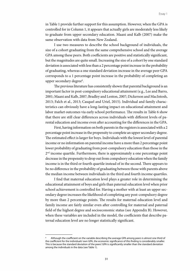
31

Essay 1

in Table 1 provide further support for this assumption. However, when the GPA is controlled for in Column 1, it appears that actually girls are moderately less likely to graduate from upper secondary education. Maani and Kalb (2007) make the same observation with data from New Zealand.

I use two measures to describe the school background of individuals, the size of a cohort graduating from the same comprehensive school and the average GPA among these peers. Both coefficients are positive and statistically significant, but the magnitudes are quite small. Increasing the size of a cohort by one standard deviation is associated with less than a 2 percentage point increase in the probability of graduating, whereas a one standard deviation increase in the average peer GPA corresponds to a 1 percentage point increase in the probability of completing an upper secondary degree6.

The previous literature has consistently shown that parental background is an important factor in post-compulsory educational attainment (e.g., Lee and Barro, 2001; Maani and Kalb, 2007; Bradley and Lenton, 2007; Dickerson and MacIntosh, 2013; Falch et al., 2013; Casquel and Uriel, 2015). Individual and family charac-teristics can obviously have a long-lasting impact on educational attainment and labor market outcomes via early school performance. The results in Table 6 show that there are still clear differences across individuals with different levels of pa-rental education and income even after accounting for the differences in the GPA.

First, having information on both parents in the registers is associated with a 2 percentage point increase in the propensity to complete an upper secondary degree. The estimated effect is larger for boys. Individuals with the lowest level of parental income or no information on parental income have a more than 2 percentage point lower probability of graduating from post-compulsory education than those in the 2nd income quartile. Furthermore, there is approximately a one percentage point decrease in the propensity to drop out from compulsory education when the family income is in the third or fourth quartile instead of in the second. There appears to be no difference in the probability of graduating between those with parents above the median income between individuals in the third and fourth income quartiles.

I find that maternal education level plays a greater role in determining the educational attainment of boys and girls than paternal education level when prior school achievement is controlled for. Having a mother with at least an upper sec-ondary degree increases the likelihood of completing any post-compulsory degree by more than 2 percentage points. The results for maternal education level and family income are fairly similar even after controlling for maternal and paternal field of the highest degree and socioeconomic status (see Appendix B). However, when these variables are included in the model, the coefficients that describe pa-ternal education level are no longer statistically significant.

6 Although the coefficient on the variable describing the average GPA among peers is almost one third of the coefficient for the individuals’ own GPA, the economic significance of this finding is considerably smaller. This is because the standard deviation of the peers’ GPA is significantly smaller than the standard deviation among the individuals in the data (see Table 1).

32

Essay 1

Finally, the results show that boys who graduated from compulsory education between 2001 and 2003 are approximately 2 percentage points more likely to complete an upper secondary degree than those who graduated in 2000. The year 2000 also experienced the largest cohort, 65,100. This is significantly larger than what is observed for the other years, which varied from 59,800 in 2003 to 62,800 in 2001. As the overall number of open schooling positions was not adjusted, that is, the number of slots per person was 1.37 in 2000 compared to the 1.43–1.49 in 2001-2003, the estimated higher propensity to drop out for the year 2000 cohort may pick up some crowding effects7. The results on other supply-side instruments are discussed in detail in Section 5.2.

As prior achievement is such a strong determinant of upper secondary edu-cation attainment, I run the regressions separately for individuals in different GPA quartiles. The estimates for individual characteristics are reported in Appendix C. The results show that the findings in Table 6 are mainly driven by individuals with low or mediocre prior achievement. Apart from age and nationality at the end of compulsory education, hardly anything appears to affect the probability of graduating for high achievers. These individuals have, on average, a completion rate of 98.9 percent. The corresponding figures are 69.2, 86.6, and 95.5 percent for the first, second, and third GPA quartiles, respectively.

6.2. Availability of education

There are at least two ways regional constraints on education supply may influence the probability of completing an upper secondary degree. First, the distance to supply may affect the expected costs of education and, thus, the initial participation decision8. Furthermore, the proximity to supply is likely to affect the distance to the school in which individual enrolls, and thus, it may induce an individual to drop out from education.

Falch et al. (2013) finds that increasing travel time to the nearest upper sec-ondary education alternative by half an hour decreases the probability of graduating on time by a little more than 2 percentage points in Norway. I perform a similar analysis and estimate how the availability of an upper secondary alternative in the municipality of residence is associated with the probability an individual will complete a post-compulsory degree within nine years after leaving compulsory education. The results reported in the first row in Table 8 show that there is a 2.6 percent increase in the probability of graduating from an upper secondary educa-tion if an alternative is provided in the municipality of residence. The association

7 Although the overall number of open slots per cohort appears to be sufficiently high for all the observa-tion years, the regional division of these slots and the individuals graduating from compulsory education may not have been matched perfectly. Furthermore, there are always many of those from the previous cohorts par-ticipating in the joint application system, and thus, the final number of open slots for each new cohort can cer-tainly be inadequate.

8 Card (2001) reviews the literature that explores proximity to education as an instrument for education participation decision.

33

Essay 1

is, however, positive only for boys and has actually a very large negative coefficient for girls. Table 9 presents the findings for the sub-samples split into four groups according to prior achievement. The availability of an upper secondary school alternative has a large positive association with the probability of graduating for individuals in the first GPA quartile and an equally large negative association with the probability of graduating for those in the third quartile. These findings show that the link between the regional supply of education and the dropout probability is not straightforward.

Dickerson and MacIntosh (2013) examine how distance to the nearest insti-tution providing post-compulsory education influences the probability of being enrolled in an upper secondary institution one year after leaving compulsory education in the United Kingdom. They found that distance matters only for indi-viduals with mediocre prior school performance and a disadvantaged background. Furthermore, they observed that the distance to different education tracks (aca-demic and vocational) may have different impacts on the participation decision.

In most countries, upper secondary education contains a set of distinct education alternatives, and it may make a big difference to individuals which education alternative is provided nearby. Tables 8 and 9 report the estimates from a specification where I determine the availability of upper secondary education in the municipality and in the sub-region (conditional on not being offered in the municipality of residence) for each education field separately. These results show that there are large differences in how the supply of different education alterna-tives is linked to the probability of graduating. Furthermore, the availability of the education alternatives appears to have a very heterogeneous effect on different subgroups of individuals.

Boys who have a high school or a vocational cultural school available in their municipality of residence appear to be approximately 2 percentage points less likely to complete a post-compulsory degree than their counterparts in mu-nicipalities where these fields are not provided. However, the supply of the field administration and commerce has a 5 percentage point positive association with the probability of completing a degree. For girls, only the proximity to the field of culture has a statistically significant positive link to the propensity to complete an upper secondary degree.

There is also a lot of heterogeneity in the estimates for individuals in dif-ferent GPA quartiles reported in Table 9. It appears that having a high school in the municipality of residence increases the dropout rate for individuals in the second GPA quartile by almost 4 percentage points, whereas for this subgroup the availability of administration and commerce has a large, close to 9 percentage point, positive association with the probability of completing a post-compulsory degree. For those in the lowest GPA quartile, the supply of social and health care service education in the municipality has a 2.5 percentage point positive influence on educational attainment. The presence of the field humanities and teaching in the municipality or in the sub-region is linked to a higher probability of dropping out for individuals with a less than median GPA.

34

Essay 1

A problem in interpreting these estimates is that the influence of distance to education on the probability of completing a degree may be entangled with the impact of the choice of education track. Kelchtermans and Verboven (2010), who studied tertiary education choices, showed that travel costs affect the choice of what and where to study more than the decision to enroll in a university. In another study (Virtanen and Väänänen, 2015), similar results for the influence of regional constraints on upper secondary education choice were found. The present study (a work in progress) examines how the regional supply of education affects the demand for the upper secondary education fields and for the outside option of not applying to post-compulsory educational institutions. We find that application decisions are sensitive to the two supply measures we use: distance to the nearest municipality offering an education field and the number of open positions per cohort in the field in the sub-region. Sensitivity to the supply depends strongly on an individual’s GPA, as do the substitution patterns. We use the demand estimates to investigate a counterfactual scenario of no distance constraints and find that a substantial fraction of individuals would move away from the choices of high school and not applying and apply to the vocational fields instead. The results in-dicate that institutional factors have a significant impact on application decisions and consequently on the sorting of individuals into different education tracks.

As can be seen in Table 5, there are large differences in the probability of graduating across different education fields. Thus, the education supply may also have an indirect link to the probability of graduating via the choice of an education field. To disentangle the influence of proximity to an educational institution on dropout behavior, I estimate how the closeness to the education choice where an individual is actually enrolled plays a role in determining the propensity to drop out.

The specification used for the results in Table 10 takes into account the field of education as well as the choice of not being enrolled in upper secondary education immediately after the end of compulsory education (the results for these variables are discussed in Section 5.3.). Thus, the dummy variable that has a value of 1 if an individual is enrolled in a municipality other than his or her municipality of resi-dence at the end of compulsory education describes the difference between those enrolled in their initial municipality of residence and those enrolled somewhere further away. This should give more insight into the influence of distance to edu-cation on the probability of completing an upper secondary degree.

The estimates on this location dummy are reported in the first row in Table 10. The results show that there is a statistically significant negative effect of being enrolled outside the initial home municipality for all GPA quartiles. The probability of graduating from an upper secondary education is approximately 2 percentage points higher for those from the first three GPA quartiles enrolled in their mu-nicipality of residence compared to their counterparts enrolled further away. For individuals with higher prior achievement, the distance to education has a smaller influence on the dropout probability.

Table 4 showed that the likelihood of choosing an education alternative outside the municipality of residence sharply decreases in the availability of upper

35

Essay 1

secondary educational alternatives. Thus, the lack of regional supply is most likely a key factor in increasing distance to education that again appears to lead to an increase in the probability of dropping out.

6.3. Field of education

The negative association between the availability of upper secondary educational alternatives and the probability of completing a post-compulsory degree among individuals with low prior achievement presented in the previous section suggests that some education fields might not be an optimal match for these individuals. Here, I explore directly the importance of the chosen education field on the pro-pensity to drop out across sub-groups with different levels of prior achievement.

The results in Table 10 show that enrollment in vocational education instead of high school the first autumn of entering upper secondary education is positively associated with the probability of completing any post-compulsory education for the individuals in the two lowest GPA quartiles. The impact is particularly large, varying between 10 and 20 percentage points, for those in the first GPA quartile. Instead, the two upper GPA quartiles perform better in high school than in most of the vocational fields. The same is depicted in Figure 1 that plots the mean graduation rate across the bins divided based on the GPA separately for those who are enrolled in high school, who are enrolled in vocational education, or who are outside of education the first autumn after leaving compulsory education. The probability of graduating appears to be again higher in high school than in vocational education only for individuals with an above median GPA in comprehensive schooling.

These results are in line with the findings in Hall (2009, 2012) that show that adding academic content to all vocational tracks in Sweden in the 1990s increased the probability of dropping out for those with low school performance. Similarly, Goux et al. (2014) find that an experiment carried out in France that led low-achieving individuals to apply more often to vocational tracks instead of more selective academic programs also decreased the repetition and dropout propensity for these individuals.

Finally, the last row in Table 10 shows that having a gap year after compulsory education (being outside of education in the autumn) is a strong predictor of failure to complete any upper secondary education. Table 11 presents the distribution of education choices across the GPA quartiles and gives a sense of the economic im-portance of the results reported in Table 10. It is clear that below the median GPA where the percentage of individuals not enrolled in additional study immediately after the end of compulsory education is non-negligible, but the 5 to 15 percentage point decrease in the probability of ever graduating poses a reason to worry.

In another study (Virtanen and Väänänen, 2015), we showed that the percentage of individuals with low prior school performance who apply to high school as their first request or who choose an outside option of not applying to an upper secondary institution would have been reduced by close to 10 percent by

36

Essay 1

improving the availability of vocational fields. Thus, at least part of the estimated influence of the education field choice on the dropout rate may be driven by re-gional supply constraints.

7. DISCUSSIONThis study explored the determinants of dropping out of post-compulsory educa-tion in Finland. The study is motivated by previous research that has convincingly shown that the failure to complete an upper secondary degree is disadvantageous to the individual in question and society alike (e.g., Card, 2001; Lochner, 2011; Grossman, 2006).

I find that early education performance in general has great importance in determining the probability of completing an upper secondary degree. That is, a low GPA in the compulsory schooling leaving certificate, the repetition of a year during comprehensive schooling, and failure to continue to upper secondary education directly after the end of compulsory education are all strongly correlated with the propensity to drop out. Furthermore, the education field choice made during the last spring semester in compulsory education is closely linked to the probability of graduating. These results suggest that the efforts to improve post-compulsory education attainment should focused on the early years of education in order to get the best results from interventions.

Similar conclusions can be reached concerning the worries raised over boys’ educational attainment (e.g., Myrskylä, 2012). According to the descriptive statistics, boys experience a significantly higher propensity to drop out from post-compulsory education. This can, however, be entirely explained by individual background characteristics and by prior school performance in particular. Thus, policy tools aimed at improving boys’ education attainment should be targeted at adolescents.

The results for the influence of the supply of upper secondary educational institutions are mixed. Availability of education is often found to be negatively associated with the probability of graduating for some sub-groups of individuals. The last set of results for the link between the education field and the probabil-ity of graduating shed light on this baffling finding. It seems that the choice of education field that is influenced by the regional supply (e.g., Klechtermans and Verboven, 2010; Virtanen and Väänänen, 2015) is an important determinant of the probability of dropping out of school. Furthermore, the findings show that the education field that experiences the lowest dropout rate varies drastically between the subgroups of individuals with different levels of prior achievement indicating that the individuals should be given considerable support and information when they are making their upper secondary education choice. This notation gets further support from the recent experiment in France (Goux et al., 2014).

37

Essay 1

REFERENCESAujeco, E. and James, J. (2015) “The path to college education: are verbal skills

more important than math skills?”, unpublished manuscript.Albaek, K., Asplund, R., Erling, B., and Lindah, L. (2015) “Youth unemployment

and inactivity: a comparison of school-to-work transitions and labour market outcomes in four Nordic countries”, Nordic Council of Ministers, Copenha-gen: Nordisk Ministerråd.

Altonji, J. G. (1993) “The Demand for and return to education when education outcomes are uncertain”, Journal of Labor Economics, 11, 48-83.

Arcidiacono, P. (2004) “Ability sorting and the return to college major”, Journal of Econometrics, 121, 343-375.

Becker, G. (1962) “Investment in human capital: a theoretical analysis”, Journal of Political Economy, 70:5, 9-49.

Becker, G. (1964) “Human capital: a theoretical and empirical analysis with special reference to education”, Columbia University Press, New York.

Belly, P. and Lochner, L. (2007) “The changing role of family income and ability in determining educational achievement”, Journal of Human Capital, 1, 37-89.

Bobonis, G.J. and Finan, F. (2009) “Neighborhood peer effects in secondary school enrollment decisions”, The Review of Economics and Statistics, 91:4, 695-716.

Bradley, S. and Lenton, P. (2007) “Dropping out post-compulsory education in the UK: an analysis of determinants and outcomes”, Journal of Population Economics, 20, 299-328.

Card, D. (2001) “Estimating the returns to schooling: progress on some persistent econometric problems”, Econometrica, 69:5, 1127-1160.

Casquel, E. and Uriel, E. (2007) “The determinants of post-compulsory education in Spain”, Applied Economics Letters, 16:4, 399-404.

Dearden, L., Emmerson, C., Frayne, C., and Meghir, C. (2009) “Conditional cash transfers and school dropout rates”, The Journal of Human Resources, 44:4, 827-857.

Dickerson, A. and McIntosh, S. (2013) “The impact of distance to nearest education institution on the post-compulsory education participation decision”, Urban Studies, 50:4, 742-758.

Eckstein, Z. and Wolpin, K.I. (1999) “Why youths drop out of high school: the im-pact of preferences, opportunities and abilities”, Econometrica, 67, 1295-1339.

Falch, T., Lujala, P., and Strom, B. (2013) “Geographical constraints and educational attainment”, Regional Science and Urban Economics, 43, 164-176.

Felgueroso, F., Gutiérrez-Domènech, M., and Jiménez-Martin, S. (2014) “Dropout trends and educational reforms: the role of the LOGSE in Spain”, IZA Journal of Labor Policy, 3:9, xx-xx.

Goux, D., Gurgand, M., and Maurin, E. (2014) “Adjusting your dreams? The effect of school and peers on dropout behaviour”, IZA Discussion Paper No. 7948.

Grossman, M. (2006) “Education and nonmarket outcomes”, Handbook of the Economics of Education, 1, 577-633.

38

Essay 1

Hall, C. (2009) “Does making upper secondary school more comprehensive affect dropout rates, educational attainment and earnings? Evidence from a Swedish pilot scheme”, Institute for Labour Market Policy Evaluation, Working paper 9.

Hall, C. (2012) “The effects of reducing tracking in upper secondary school: ev-idence from a large-scale pilot scheme”, The Journal of Human Resources, 47:1, 237-269.

Hanushek, E. (1986) “The economics of schooling: production and efficiency in public schools”, Journal of Economic Literature, 24:3, 1141-1177.

Hastings, J., Neilson, C., and Zimmerman, S. (2013) “Are some degrees worth more than others? Evidence from college admission cutoffs in Chile”, NBER Working Paper No. 19241.

Kelchtermans, S. and Verboven, F. (2010) “Participation and study decisions in a public system of higher education”, Journal of Applied Econometrics, 25, 355-391.

Kirkebøen, L., Leuven, E., and Mogstad, M. (2014) “Field of study, earnings, and self-selection”, NBER Working Paper No. 20816.

Lee, J. and Barro, J. (2001) “Schooling quality in a cross-section of countries”, Economica, 68:272, 465-488.

Lochner, L. (2011) “Non-production benefits of education: crime, health, and good citizenship”, NBER Working Paper No. 16722.

Lyche, C. (2010) “Taking on the completion challenge: a literature review on poli-cies to prevent dropout and early school leaving”, OECD Education Working Papers, No. 53, OECD Publishing.

Maani, S.A. and Kalb, G. (2007) “Academic performance, childhood, economic resources, and the choice to leave school at age 16”, Economics of Education Review, 26, 361-374.

Malamud, O. and Pop-Eleches, C. (2010) “General education versus vocational training: evidence from an economy in transition”, The Review of Economics and Statistics, 92:1, 43-60.

Maliranta, M., Nurmi, S., and Virtanen, H. (2010) “Resources in vocational edu-cation and post-schooling outcomes”, International Journal of Manpower, 31:5, 520-544.

Manski, C. F. (1989) “Schooling as experimentation: a reappraisal of the postsec-ondary dropout phenomenon”, Economics of Education Review, 8:4, 305-312.

Meschi, E., Swaffield, J., and Vignoled, A. (2011) “The Relative Importance of Lo-cal Labour Market Conditions and Pupil Attainment on Post-Compulsory Schooling Decisions”, IZA Discussion Paper No. 6143.

Micklewright, J., Pearson, M., and Smith, S. (1990) “Unemployment and early school leaving”, Economic Journal, 100:400, 163-169.

Mincer, J. (1958) “Investment in human capital and personal income distribution”, Journal of Political Economy, 66:4, 281-302.

Myrskylä, P. (2012) “Hukassa – Keitä ovat syrjäytyneet nuoret?”, EVA Analyysi 19/2012, Helsinki: Elinkeinoelämän valtuuskunta.

39

Essay 1

Oreopoulos, P. (2007) “Do dropouts drop out too soon? Wealth, health and happiness from compulsory education”, Journal of Public Economics, 91, 2213-2229.

Reyes, L., Rodrigues, J., and Urzula, S. (2013) “Heterogeneous economic returns to postsecondary degrees: evidence from Chile”, NBER Working Paper No. 18817.

Rice, P. (2010) “Minimum wages and schooling: evidence from the UK’s introduc-tion of a national minimum wage”, Department of Economics, University of Oxford, April, No. 482.

Rumberger, R. and Lim, S. (2008) “Why Students Drop Out of School: A Review of 25 Years of Research”, California Dropout Research Project, Santa Barbara.

Sacerdote, B. (2011) “Peer effects in education: how might they work, how big are they and how much do we know thus far?” Handbook of the Economics of Education, 3, 249-277.

Virtanen, H. and Väänänen, L. (2015) “Regional supply and student sorting”, unpublished manuscript.

Willis, R. and Rosen, S. (1979) “Education and self-selection”, Journal of Political Economy, 87:5, S7-S36.

40

Essay 1

FIGURE

Figure 1 Likelihood of completing a post-compulsory degree conditional on GPA and initial enrollment

41

Essay 1

Table 1 Descriptive statistics of individuals’ background characteristics

Total data Total sampleDegree in

9 years

No degree in

9 yearsDiff

Completed an upper secondary degree in 9 years 86.9 88.0 . . .Individual characteristicsGPA 7.6 (1.1) 7.7 6,5 1.2***Disabilities 6.6 6.5 7.5 -1.0***Age at graduation from compulsory education 16.1 (0.3) 16.1 (0.3) 16.0 16.2 -0.2***Nationality Finnish 98.2 98.3 98.6 96.1 2.5***Mother tongue Finnish 92.7 92.8 92.9 91.9 1.0***Mother tongue Swedish 5.2 5.3 5.5 3.7 1.9***Mother tongue other than the two official languages 2.1 2.0 1.6 4.5 -2.9***Male 51.0 50,1 49,4 62.2 -12.8***Mean characteristics of comprehensive schoolSize (no of peers in the data) 110 (48) 110 (47) 111 105 6.2***Average GPA among peers 7.6 (0.3) 7.6 (0.3) 7.6 7.5 0.1***Year graduating from comprehensive schoolYear 2000 26.2 26.3 26.0 27.8 -1.8***Year 2001 25.3 25.2 25.3 24.9 0.4Year 2002 24.4 24.4 24.4 24.2 0.2Year 2003 24.1 24.4 24.3 23.1 1.1***Family backgroundInformation on both parents available 67.9 68.3 71.0 48.8 22.3***Information on both parents missing 11.5 11.3 10.1 19.8 -9.7***Family income € 44,891 (27,086) 45,102 (27,051) 46,453 34,061 12,392***Level of father's educationNo post-compulsory degree or infromation missing 45.8 45.4 42.7 65.1 -22.4***Upper secondary degree 39.9 40.2 41.6 39.0 11.5***Tertiary degree 14.3 14.4 15.7 4.8 10.9***Level of mother's educationNo post-compulsory degree or infromation missing 29.7 29.2 26.6 48.3 -21.6***Upper secondary degree 57.0 57.3 58.8 46.7 12.1***Tertiary degree 13.3 13.4 14.6 5.0 9.5***N 248 094 242 566 213 248 29 196

Sample used in the main analysis

TABLES

42

Essay 1

Table 1 cont’d

Total data Total sampleDegree in

9 years

No degree in

9 yearsDiff

Field of father's educationHigh school 1.7 1.7 1.8 1.4 0.4***Natural Science 6.5 6.5 7.0 3.2 3.7***Technology and Transport 32.0 32.2 33.5 22.9 10.6***Administration and Commerce 7.0 7.0 7.5 3.6 3.8***Hotel, Catering and Home Economics 0.7 0.7 0.7 0.7 0.0Social and Health Care Services 2.2 2.2 2.4 1.0 1.4***Culture 0.5 0.5 0.5 0.4 0.1***Humanities and Teaching 2.0 2.0 2.1 0.7 1.4***Field of mother's educationHigh school 2.5 2.5 2.6 2.2 0.4***Natural Science 2.7 2.8 2.9 1.5 1.4***Technology and Transport 6.3 6.3 6.4 5.8 0.5***Administration and Commerce 18.7 18.8 19.7 12.5 7.2***Hotel, Catering and Home Economics 10.9 10.9 10.9 10.7 0.2Social and Health Care Services 21.7 21.9 22.7 15.6 7.2***Culture 1.3 1.3 1.3 1.0 0.3***Humanities and Teaching 6.1 6.2 6.7 2.2 4.5***Father's socioeconomic statusUpper level employee 14.5 14.6 15.8 5.7 10.2***Lower level employee 12.7 12.8 13.4 8.2 5.2***Manual worker 23.1 23.2 23.4 22.1 1.3***Self-employed 12.6 12.7 13.3 8.3 5.1***Outside of labour force (e.g. student, pensioner) 7.2 7.2 7.0 8.7 -1.7***Information on socioeconomic status missing 30.0 29.5 27.0 47.1 -20.1***Mother's socioeconomic statusUpper level employee 13.5 12.6 14.7 5.5 9.2***Lower level employee 33.3 33.6 34.7 25.1 9.6***Manual worker 16.2 16.2 15.8 19.4 -3.6***Self-employed 8.5 8.5 8.9 5.7 3.2***Outside of labour force (e.g. student, pensioner) 11.5 11.4 10,8 15,9 -5.1***Information on socioeconomic status missing 16.9 16.6 15.0 28.4 -13.3***N 248 094 242 566 213 248 29 196

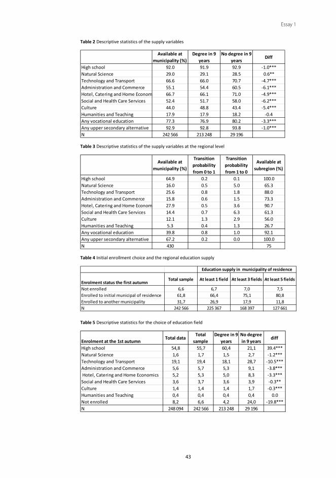
43

Essay 1

Table 2 Descriptive statistics of the supply variables

Table 3 Descriptive statistics of the supply variables at the regional level

Table 4 Initial enrollment choice and the regional education supply

Available at municipality (%)

Degree in 9 years

No degree in 9 years

Diff

High school 92.0 91.9 92.9 -1.0***Natural Science 29.0 29.1 28.5 0.6**Technology and Transport 66.6 66.0 70.7 -4.7***Administration and Commerce 55.1 54.4 60.5 -6.1***Hotel, Catering and Home Econom 66.7 66.1 71.0 -4.9***Social and Health Care Services 52.4 51.7 58.0 -6.2***Culture 44.0 48.8 43.4 -5.4***Humanities and Teaching 17.9 17.9 18.2 -0.4Any vocational education 77.3 76.9 80.2 -3.3***Any upper secondary alternative 92.9 92.8 93.8 -1.0***N 242 566 213 248 29 196

Available at municipality (%)

Transition probability from 0 to 1

Transition probability from 1 to 0

Available at subregion (%)

High school 64.9 0.2 0.1 100.0Natural Science 16.0 0.5 5.0 65.3Technology and Transport 25.6 0.8 1.8 88.0Administration and Commerce 15.8 0.6 1.5 73.3Hotel, Catering and Home Econom 27.9 0.5 3.6 90.7Social and Health Care Services 14.4 0.7 6.3 61.3Culture 12.1 1.3 2.9 56.0Humanities and Teaching 5.3 0.4 1.3 26.7Any vocational education 39.8 0.8 1.0 92.1Any upper secondary alternative 67.2 0.2 0.0 100.0N 430 75

Enrolment status the first autumnTotal sample At least 1 field At least 3 fields At least 5 fields

Not enrolled 6,6 6,7 7,0 7,5Enrolled to initial municipal of residence 61,8 66,4 75,1 80,8Enrolled to another municipality 31,7 26,9 17,9 11,8N 242 566 225 367 168 397 127 661

Education supply in municipality of residence

Table 5 Descriptive statistics for the choice of education field

Enrolment at the 1st autumnTotal data

Total sample

Degree in 9 years

No degree in 9 years

diff

High school 54,8 55,7 60,4 21,1 39.4***Natural Science 1,6 1,7 1,5 2,7 -1.2***Technology and Transport 19,1 19,4 18,1 28,7 -10.5***Administration and Commerce 5,6 5,7 5,3 9,1 -3.8*** Hotel, Catering and Home Economics 5,2 5,3 5,0 8,3 -3.3***Social and Health Care Services 3,6 3,7 3,6 3,9 -0.3**Culture 1,4 1,4 1,4 1,7 -0.3***Humanities and Teaching 0,4 0,4 0,4 0,4 0.0Not enrolled 8,2 6,6 4,2 24,0 -19.8***N 248 094 242 566 213 248 29 196

44

Essay 1

Table 6 Estimates of individuals’ background characteristics

Total sample

Boys GirlsTotal

sampleTotal data

Individual characteristicsGPA 0.092*** 0.097*** 0.086***

(0.003) (0.004) (0.003)Disabilities 0.001 0.009** -0.009***

(0.003) (0.004) (0.004)Under 16 years old 0 0 0 0 016 years old 0.005 0.010 0.003 -0.030*** -0.033***

(0.004) (0.009) (0.005) (0.004) (0.005)Over 16 years old -0.123*** -0.110*** -0.136*** -0.214*** -0.235***

(0.005) (0.010) (0.007) (0.006) (0.006)Nationality Finnish 0.031*** 0.058*** 0.006 0.034*** 0.047***

(0.011) (0.016) (0.013) (0.011) (0.012)Mother tongue Finnish 0 0 0 0 0Mother tongue Swedish 0.045*** 0.048*** 0.043*** 0.036*** 0.040***

(0.010) (0.012) (0.009) (0.008) (0.009)Mother tongue other than the two official languages -0.003 0.007 -0.008 -0.001 0.006

(0.012) (0.013) (0.014) (0.011) (0.011)Male 0.007*** -0.046*** -0.046***

(0.002) (0.002) (0.002)Characteristics of comprehensive schoolSize (10x no of peers in the data) 0.004*** 0.004*** 0.003*** 0.003*** 0.003***

(0.004) (0.005) (0.004) (0.003) (0.003)Average GPA among peers 0.028*** 0.035*** 0.019*** 0.088*** 0.089***

(0.006) (0.007) (0.006) (0.005) (0.006)Year graduating from comprehensive schoolYear 2000 0 0 0 0 0Year 2001 0.011*** 0.019*** 0.004* 0.010*** 0.010***

(0.002) (0.003) (0.002) (0.002) (0.002)Year 2002 0.010*** 0.019*** 0.001 0.008*** 0.008***

(0.002) (0.003) (0.003) (0.002) (0.002)Year 2003 0.012*** 0.021*** 0.003 0.010*** 0.010***

(0.002) (0.004) (0.003) (0.002) (0.002)N 242 566 123 604 118 962 242 566 247 552Note: All specifications include the supply side variables reported in Table 7 (specification 2) and municipality dummies. Standard errors clustered on municipality level shown in parenthesis. ***significant at 10%, **significant at 5%, *significant at 1%

45

Essay 1

Table 6 cont’d

Total sample

Boys GirlsTotal

sampleTotal data

Family backgroundInformation on both parents available 0.020*** 0.027*** 0.013*** 0.015*** 0.015***

(0.003) (0.004) (0.003) (0.004) (0.004)Family income in 1st quartile or information missing 0 0 0 0 0Family income in 2nd quartile 0.026*** 0.022*** 0.031*** 0.033*** 0.037***

(0.003) (0.003) (0.003) (0.003) (0.003)Family income in 3rd quartile 0.038*** 0.036*** 0.040*** 0.051*** 0.056***

(0.003) (0.004) (0.004) (0.004) (0.004)Family income in 4th quartile 0.039*** 0.036*** 0.044*** 0.064*** 0.070***

(0.003) (0.004) (0.004) (0.004) (0.004)Level of father's educationNo post-compulsory degree or infromation missing 0 0 0 0 0Upper secondary degree 0.009*** 0.016*** 0.002 0.023*** 0.024***

(0.002) (0.003) (0.002) (0.002) (0.002)Tertiary degree -0.001 0.005 -0.008*** 0.047*** 0.049***

(0.003) (0.004) (0.003) (0.003) (0.003)Level of mother's educationNo post-compulsory degree or infromation missing 0 0 0 0 0Upper secondary degree 0.027*** 0.030*** 0.024*** 0.045*** 0.047***

(0.002) (0.003) (0.003) (0.003) (0.003)Tertiary degree 0.024*** 0.031*** 0.017*** 0.074*** 0.078***

(0.003) (0.004) (0.003) (0.004) (0.005)

Constant -0.151** -0.284*** 0.014 0.130** 0.091

(0.067) (0.072) (0.087) (0.054) (0.058)N 242 566 123 604 118 962 242 566 247 552Note: All specifications include the supply side variables reported in Table 7 (specification 2) and municipality dummies. Standard errors clustered on municipality level shown in parenthesis. ***significant at 10%, **significant at 5%, *significant at 1%

Table 7 Estimates of subject grades

All All Boys GirlsPrior school performanceGPA 0.083***

-0.003Native language 0.047*** 0.045*** 0.050***

(0.002) (0.002) (0.002)Math 0.024*** 0.028*** 0.019***

(0.001) (0.002) (0.002)Music 0.000 0.004*** 0.005*** 0.002

(0.001) (0.001) (0.002) (0.002)Sport education 0.034*** 0.037*** 0.029*** 0.050***

(0.001) (0.001) (0.002) (0.002)Arts 0.012*** 0.015*** 0.017*** 0.010***

(0.002) (0.002) (0.002) (0.003)Handcraft 0.029*** 0.031*** 0.037*** 0.023***

(0.001) (0.001) (0.002) (0.002)Constant -0.656*** -0.756*** -0.845*** -0.623***

(0.085) (0.081) (0.081) (0.114)N 173 789 173 789 96 203 77 586Note: All specifications include the full set of individual and parental characteristics, year dummies, supply side variables and municipality dummies as the regressions reported in Tables 5 and 7 (specification 2). Standard errors clustered on municipality level shown in parenthesis. ***significant at 10%, **significant at 5%, *significant at 1%

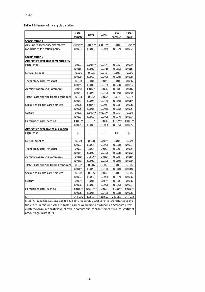
46

Essay 1

Table 8 Estimates of the supply variables

Total sample

Boys GirlsTotal

sampleTotal data

Sepcification 10.026*** 0.100*** -0.067*** -0.001 -0.020***(0.003) (0.003) (0.003) (0.002) (0.002)

Specification 2Alternative available at municipalityHigh school 0.001 -0.016** 0.017 0.005 0.009

(0.015) (0.007) (0.031) (0.015) (0.016)Natural Science -0.006 -0.021 0.012 -0.006 -0.005

(0.008) (0.019) (0.008) (0.008) (0.008)Technology and Transport -0.003 0.001 -0.015 -0.001 0.006

(0.025) (0.030) (0.022) (0.023) (0.023)Administration and Commerce 0.020 0.047* -0.006 0.018 0.016

(0.021) (0.026) (0.029) (0.019) (0.020) Hotel, Catering and Home Economics -0.014 -0.022 -0.000 -0.014 -0.017

(0.021) (0.024) (0.018) (0.019) (0.019)Social and Health Care Services 0.008 0.014* 0.003 0.008 0.008

(0.005) (0.008) (0.005) (0.005) (0.005)Culture 0.001 -0.020** 0.022** 0.001 -0.002

(0.007) (0.010) (0.009) (0.007) (0.007)Humanities and Teaching -0.011** -0.016* -0.004 -0.012** -0.011**

(0.005) (0.009) (0.006) (0.005) (0.005)Alternative available at sub-regionHigh school (.) (.) (.) (.) (.)

Natural Science -0.004 -0.020 0.015* -0.004 -0.003(0.007) (0.018) (0.009) (0.008) (0.007)

Technology and Transport 0.001 0.014 -0.021 0.000 0.005(0.024) (0.029) (0.020) (0.023) (0.022)

Administration and Commerce 0.020 0.051** -0.010 0.020 0.019(0.021) (0.026) (0.028) (0.019) (0.020)

Hotel, Catering and Home Economics -0.007 -0.016 0.009 -0.008 -0.009(0.019) (0.023) (0.017) (0.018) (0.018)

Social and Health Care Services -0.008 -0.005 -0.007 -0.008 -0.009(0.007) (0.012) (0.006) (0.007) (0.006)

Culture 0.009 0.001 0.015* 0.008 0.006(0.006) (0.009) (0.009) (0.006) (0.007)

Humanities and Teaching -0.018** -0.031*** -0.003 -0.018** -0.016**(0.008) (0.008) (0.010) (0.008) (0.008)

N 242 566 123 604 118 962 242 566 247 552Note: All specifications include the full set of individual and parental characteristics and the year dummies reported in Table 5 as well as municipality dummies. Standard errors clustered on municipality level shown in parenthesis. ***significant at 10%, **significant at 5%, *significant at 1%

Any upper secondary alternative available at the municipality

47

Essay 1

Table 9 Estimates of the supply variables across the GPA quartiles

Total sample

GPA in 1st

quartile

GPA in 2nd

quartile

GPA in 3rd

quartile

GPA in 4th

quartileSepcification 1

0.026*** 0.079*** 0.023*** -0.084*** 0.004***(0.003) (0.006) (0.005) (0.004) (0.001)

Specification 2Alternative available at municipalityHigh school 0.001 0.048 -0.037** -0.005 -0.005

(0.015) (0.053) (0.017) (0.009) (0.007)Natural Science -0.006 -0.001 0.005 -0.016** -0.002

(0.008) (0.029) (0.021) (0.008) (0.006)Technology and Transport -0.003 -0.005 -0.031 0.036 -0.014

(0.025) (0.067) (0.037) (0.022) (0.019)Administration and Commerce 0.020 -0.035 0.089* -0.003 0.006

(0.021) (0.053) (0.048) (0.019) (0.006) Hotel, Catering and Home Economics -0.014 0.004 -0.023 -0.019 -0.005

(0.021) (0.045) (0.037) (0.018) (0.006)Social and Health Care Services 0.008 0.025* 0.001 0.006 0.000

(0.005) (0.013) (0.013) (0.005) (0.004)Culture 0.001 -0.007 0.012 -0.007 -0.002

(0.007) (0.018) (0.015) (0.011) (0.005)Humanities and Teaching -0.011** -0.011 -0.030 0.002 0.005*

(0.005) (0.018) (0.026) (0.008) (0.003)Alternative available at sub-regionHigh school (.) (.) (.) (.) (.)

Natural Science -0.004 0.012 -0.006 -0.010 -0.004(0.007) (0.029) (0.021) (0.007) (0.005)

Technology and Transport 0.001 0.022 -0.031 0.011 -0.009(0.024) (0.062) (0.035) (0.019) (0.019)

Administration and Commerce 0.020 0.009 0.065 -0.003 0.002(0.021) (0.051) (0.046) (0.018) (0.006)

Hotel, Catering and Home Economics -0.007 0.004 0.001 -0.001 -0.010*(0.019) (0.046) (0.032) (0.016) (0.005)

Social and Health Care Services -0.008 -0.019 -0.025* 0.005 -0.003(0.007) (0.024) (0.014) (0.008) (0.006)

Culture 0.009 0.018 0.022 -0.009 0.001(0.006) (0.018) (0.014) (0.010) (0.005)

Humanities and Teaching -0.018** -0.019 -0.026 -0.004 -0.010(0.008) (0.016) (0.019) (0.013) (0.007)

N 242 566 55 962 63 983 59 250 63 371Note: All specifications include the full set of individual and parental characteristics and the year dummies reported in Table 5 as well as municipality dummies. Standard errors clustered on municipality level shown in parenthesis. ***significant at 10%, **significant at 5%, *significant at 1%

Any upper secondary alternative available at the municipality

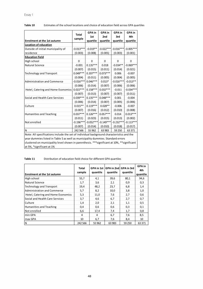
48

Essay 1

Table 10 Estimates of the school locations and choice of education field across GPA quartiles

Enrolment at the 1st autumn

Total sample

GPA in 1st

quartile

GPA in 2nd

quartile

GPA in 3rd

quartile

GPA in 4th

quartileLocation of education

-0.013*** -0.019** -0.022*** -0.016*** -0.005***(0.003) (0.008) (0.005) (0.003) (0.001)

Education fieldHigh school 0 0 0 0 0Natural Science -0.001 0.135*** 0.018 -0.034** -0.069***

(0.007) (0.015) (0.011) (0.014) (0.021)Technology and Transport 0.049*** 0.207*** 0.073*** 0.006 -0.007

(0.004) (0.011) (0.005) (0.004) (0.005)Administration and Commerce -0.016*** 0.046*** 0.013* -0.016*** -0.013**

(0.006) (0.014) (0.007) (0.006) (0.006) Hotel, Catering and Home Economics 0.022*** 0.158*** 0.032*** -0.011 -0.034***

(0.007) (0.013) (0.007) (0.007) (0.011)Social and Health Care Services 0.039*** 0.135*** 0.048*** 0.001 -0.004

(0.006) (0.014) (0.007) (0.005) (0.006)Culture 0.015** 0.119*** 0.028** -0.006 -0.007

(0.007) (0.016) (0.012) (0.010) (0.008)Humanities and Teaching 0.037*** 0.126*** 0.057*** 0.014 0.013***

(0.011) (0.023) (0.015) (0.013) (0.002)Not enrolled -0.196*** -0.052*** -0.149*** -0.232*** -0.113***

(0.007) (0.014) (0.010) (0.018) (0.017)N 242 566 55 962 63 983 59 250 63 371

Outside of initial municipality of residence

Note: All specifications include the set of individual background characteristics and the year dummies listed in Table 5 as well as municipality dummies. Standard errors clustered on municipality level shown in parenthesis. ***significant at 10%, **significant at 5%, *significant at 1%

Table 10 Distribution of education field choice for different GPA quartiles

Enrolment at the 1st autumn

Total sample

GPA in 1st quantile

GPA in 2nd quantile

GPA in 3rd quantile

GPA in 4th

quantileHigh school 55,7 4,1 39,6 80,1 94,6Natural Science 1,7 3,6 2,1 0,9 0,3Technology and Transport 19,4 48,2 23,7 6,8 1,4Administration and Commerce 5,7 8,2 10,0 3,8 1,0 Hotel, Catering and Home Economics 5,3 11,0 7,6 2,7 0,6Social and Health Care Services 3,7 4,6 6,7 2,7 0,7Culture 1,4 2,0 2,1 1,1 0,5Humanities and Teaching 0,4 0,6 0,6 0,3 0,1Not enrolled 6,6 17,4 7,4 1,7 0,8min GPA 4 4 6,7 7,6 8,5max GPA 10 6,7 7,6 8,4 10N 242 566 55 962 63 983 59 250 63 371

1

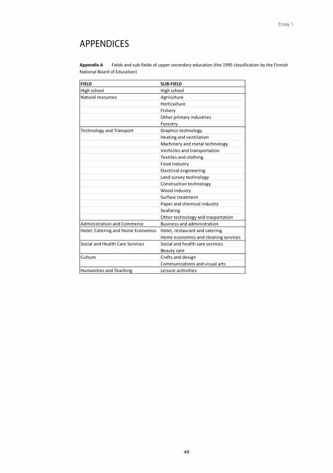
49

Essay 1

Appendix A Fields and sub-fields of upper secondary education (the 1995 classification by the Finnish National Board of Education)

FIELD SUB-FIELD High school High schoolNatural resources Agriculture

HorticultureFisheryOther primary industriesForestry

Technology and Transport Graphics technologyHeating and ventilationMachinery and metal technologyVechicles and transportationTextiles and clothingFood industryElectrical engineeringLand survey technologyConstruction technologyWood industrySurface treatmentPaper and chemical industrySeafaringOther technology and trasportation

Administration and Commerce Business and administrationHotel, restaurant and cateringHome economics and cleaning servicesSocial and health care servicesBeauty care

Culture Crafts and designCommunications and visual arts

Humanities and Teaching Leisure acitivities

Hotel, Catering and Home Economics

Social and Health Care Services

APPENDICES

50

Essay 1

Appendix B Full set of family background controls

Total sample

Boys GirlsTotal

sampleTotal data

Individual characteristicsGPA 0.092*** 0.097*** 0.086***

(0.003) (0.004) (0.003)Disabilities 0.002 0.009** -0.009**

(0.003) (0.004) (0.004)Under 16 years old 0 0 0 0 016 years old 0.005 0.009 0.003 -0.028*** -0.031***

(0.004) (0.009) (0.005) (0.004) (0.005)Over 16 years old -0.123*** -0.110*** -0.135*** -0.209*** -0.230***

(0.005) (0.010) (0.007) (0.006) (0.006)Nationality Finnish 0.031*** 0.057*** 0.005 0.034*** 0.047***

(0.011) (0.016) (0.014) (0.011) (0.012)Mother tongue Finnish 0.000 0.000 0.000 0.000 0.000Mother tongue Swedish 0.044*** 0.047*** 0.041*** 0.032*** 0.036***

(0.010) (0.012) (0.009) (0.008) (0.009)Mother tongue other than the two official languages 0.002 0.011 -0.005 0.006 0.014

(0.012) (0.014) (0.014) (0.011) (0.011)Male 0.007*** -0.046*** -0.046***

(0.002) (0.002) (0.002)Characteristics of comprehensive schoolSize (10x no of peers in the data) 0.004*** 0.004*** 0.003*** 0.003*** 0.032***

(0.004) (0.005) (0.004) (0.003) (0.003)Average GPA among peers 0.029*** 0.035*** 0.020*** 0.086*** 0.087***

(0.006) (0.007) (0.006) (0.005) (0.006)Year graduating from comprehensive schoolYear 2000 0 0 0 0 0Year 2001 0.011*** 0.019*** 0.004* 0.010*** 0.010***

(0.002) (0.003) (0.002) (0.002) (0.002)Year 2002 0.010*** 0.019*** 0.001 0.008*** 0.009***

(0.002) (0.003) (0.003) (0.002) (0.002)Year 2003 0.012*** 0.021*** 0.003 0.010*** 0.011***

(0.002) (0.004) (0.003) (0.002) (0.002)Family backgroundInformation on both parents available 0.019*** 0.021*** 0.017*** 0.026*** 0.028***

(0.004) (0.006) (0.005) (0.004) (0.004)Family income in 1st quartile or information missing 0 0 0 0 0Family income in 2nd quartile 0.025*** 0.020*** 0.030*** 0.034*** 0.038***

(0.003) (0.004) (0.003) (0.003) (0.003)Family income in 3rd quartile 0.035*** 0.033*** 0.038*** 0.049*** 0.054***

(0.003) (0.005) (0.004) (0.004) (0.004)Family income in 4th quartile 0.038*** 0.035*** 0.041*** 0.055*** 0.060***

(0.003) (0.005) (0.005) (0.004) (0.005)N 242 444 123 526 118 918 242 444 247 390

51

Essay 1

Appendix B cont’d

Total sample

Boys GirlsTotal

sampleTotal data

Level of father's educationNo post-compulsory degree or infromation missing 0 0 0 0 0Upper secondary degree -0.007 -0.009 -0.004 0.020*** 0.020***

(0.005) (0.008) (0.005) (0.006) (0.005)Tertiary degree -0.009** -0.004 -0.014*** 0.036*** 0.039***

(0.004) (0.006) (0.005) (0.004) (0.004)Level of mother's educationNo post-compulsory degree or infromation missing 0 0 0 0 0Upper secondary degree 0.020*** 0.023*** 0.017*** 0.048*** 0.047***

(0.004) (0.007) (0.005) (0.005) (0.006)Tertiary degree 0.027*** 0.042*** 0.012*** 0.084*** 0.087***

(0.003) (0.005) (0.004) (0.004) (0.004)Father's socioeconomic statusUpper level employee 0 0 0 0 0Lower level employee 0.000 -0.000 0.001 -0.002 -0.002

(0.002) (0.004) (0.003) (0.003) (0.003)Manual worker 0.006** 0.007* 0.005* -0.012*** -0.013***

(0.003) (0.004) (0.003) (0.003) (0.003)Self-employed 0.010*** 0.010** 0.010*** 0.002 0.001

(0.003) (0.005) (0.002) (0.003) (0.003)Outside of labour force (e.g. student, pensioner) -0.002 0.001 -0.005 -0.017*** -0.019***

(0.003) (0.005) (0.004) (0.003) (0.003)Information on socioeconomic status missing 0.001 -0.005 0.006 -0.003 -0.003

(0.004) (0.006) (0.005) (0.004) (0.004)Mother's socioeconomic statusUpper level employee 0 0 0 0 0Lower level employee 0.006*** 0.006* 0.007*** -0.003* -0.003*

(0.002) (0.003) (0.002) (0.002) (0.002)Manual worker -0.003 -0.003 -0.004 -0.028*** -0.029***

(0.003) (0.004) (0.003) (0.003) (0.003)Self-employed 0.013*** 0.016*** 0.010*** 0.004 0.003

(0.003) (0.004) (0.003) (0.003) (0.003)Outside of labour force (e.g. student, pensioner) -0.014*** -0.016*** -0.012*** -0.035*** -0.036***

(0.003) (0.004) (0.003) (0.003) (0.003)Information on socioeconomic status missing 0.005* 0.007 0.003 0.000 0.000

(0.003) (0.006) (0.004) (0.004) (0.004)N 242 444 123 526 118 918 242 444 247 390

52

Essay 1

Appendix B cont’d

Total sample

Boys GirlsTotal

sampleTotal data

Field of father's educationUpper secondary degree from High school 0 0 0 0 0Upper secondary degree in Natural Science 0.015*** 0.023*** 0.007 0.006 0.007

(0.005) (0.008) (0.006) (0.006) (0.005)Upper secondary degree in Technology and Transport 0.017*** 0.026*** 0.007 -0.001 -0.001

(0.005) (0.007) (0.005) (0.005) (0.005)Upper secondary degree in Administration and Commerce 0.011** 0.015** 0.006 0.005 0.005

(0.005) (0.007) (0.005) (0.005) (0.005)Upper secondary degree in Hotel, Catering and Home Economics 0.013 0.017* 0.008 -0.006 -0.007

(0.008) (0.010) (0.014) (0.009) (0.008)Upper secondary degree in Social and Health Care Services 0.009 0.010 0.006 -0.001 -0.001

(0.006) (0.009) (0.008) (0.007) (0.007)Upper secondary degree in Culture -0.016 -0.011 -0.021 -0.022* -0.021

(0.011) (0.018) (0.014) (0.013) (0.014)Upper secondary degree in Humanities and Teaching 0.014 0.034* -0.010 0.004 0.003

(0.012) (0.018) (0.013) (0.011) (0.011)Tertiary degree in Natural Science 0 0 0 0 0Tertiary degree in Technology and Transport 0.015*** 0.018*** 0.013*** 0.007** 0.006*

(0.004) (0.006) (0.004) (0.003) (0.003)Tertiary degree in Administration and Commerce 0.014*** 0.013** 0.014*** 0.002 0.002

(0.004) (0.006) (0.004) (0.004) (0.004)Tertiary degree in Hotel, Catering and Home Economics -0.010 0.059 -0.063 -0.043 -0.041

(0.086) (0.042) (0.138) (0.105) (0.106)Tertiary degree in Social and Health Care Services -0.005 -0.003 -0.009 -0.002 -0.004

(0.004) (0.007) (0.005) (0.004) (0.004)Tertiary degree in Culture 0.009 -0.009 0.023* -0.017 -0.025**

(0.011) (0.018) (0.014) (0.011) (0.012)Tertiary degree in Humanities and Teaching -0.003 -0.011 0.004 -0.012** -0.014***

(0.005) (0.007) (0.006) (0.005) (0.005)N 242 444 123 526 118 918 242 444 247 390

53

Essay 1

Appendix B cont’d

Total sample

Boys GirlsTotal

sampleTotal data

Field of mother's educationUpper secondary degree from High school 0 0 0 0 0Upper secondary degree in Natural Science 0.003 0.010 -0.004 -0.006 -0.000

(0.006) (0.010) (0.007) (0.006) (0.006)Upper secondary degree in Technology and Transport 0.012*** 0.016** 0.007 -0.006 -0.001

(0.004) (0.007) (0.005) (0.005) (0.005)Upper secondary degree in Administration and Commerce 0.008** 0.010 0.006* 0.003 0.007*

(0.004) (0.006) (0.004) (0.004) (0.004)Upper secondary degree in Hotel, Catering and Home Economics 0.012*** 0.012* 0.010** -0.009* -0.005

(0.004) (0.007) (0.005) (0.005) (0.005)Upper secondary degree in Social and Health Care Services 0.006 0.007 0.005 -0.003 0.001

(0.005) (0.007) (0.004) (0.004) (0.005)Upper secondary degree in Culture 0.005 0.017* -0.008 -0.004 0.000

(0.006) (0.009) (0.008) (0.006) (0.007)Upper secondary degree in Humanities and Teaching 0.010** 0.007 0.012** 0.017*** 0.021***

(0.005) (0.007) (0.005) (0.005) (0.006)Tertiary degree in Natural Science 0 0 0 0 0Tertiary degree in Technology and Transport 0.003 -0.004 0.009 -0.008 -0.005

(0.005) (0.007) (0.005) (0.005) (0.006)Tertiary degree in Administration and Commerce 0.006 0.004 0.008* -0.010** -0.008*

(0.004) (0.007) (0.004) (0.004) (0.004)Tertiary degree in Hotel, Catering and Home Economics 0.028*** 0.011 0.045*** -0.002 0.000

(0.011) (0.016) (0.014) (0.011) (0.011)Tertiary degree in Social and Health Care Services -0.004 -0.015*** 0.008** -0.025*** -0.024***

(0.004) (0.006) (0.004) (0.004) (0.004)Tertiary degree in Culture 0.007 -0.006 0.019* -0.022*** -0.026***

(0.008) (0.013) (0.010) (0.008) (0.010)Tertiary degree in Humanities and Teaching -0.001 -0.007 0.005 -0.011*** -0.011***

(0.003) (0.006) (0.004) (0.003) (0.003)Constant -0.154** -0.283*** 0.008 0.164*** 0.125**

(0.069) (0.073) (0.089) (0.055) (0.059)N 242 444 123 526 118 918 242 444 247 390Note: All specifications include supply side variables reported in Table 7 (specification 2) and municipality dummies. Standard errors clustered on municipality level shown in parenthesis. ***significant at 10%, **significant at 5%, *significant at 1%

54

Essay 1

Appendix C Individuals’ background characteristics across GPA quartiles

Total sample

GPA in 1st

quartile

GPA in 2nd

quartile

GPA in 3rd

quartile

GPA in 4th

quartileIndividual characteristicsGPA 0.092*** 0.222*** 0.105*** 0.062*** 0.008***

(0.003) (0.006) (0.008) (0.006) (0.001)Disabilities 0.001 -0.000 0.003 -0.000 -0.003

(0.003) (0.007) (0.005) (0.004) (0.002)Under 16 years old 0 0 0 0 016 years old 0.009*** -0.005 -0.017 0.008 0.006*

(0.004) (0.045) (0.014) (0.008) (0.004)Over 16 years old -0.119*** -0.112** -0.137*** -0.093*** -0.032***

(0.005) (0.046) (0.015) (0.011) (0.009)Nationality Finnish 0.093*** 0.098*** 0.063** 0.048** 0.075***

(0.017) (0.025) (0.029) (0.024) (0.021)Mother tongue Finnish 0 0 0 0 0Mother tongue Swedish 0.045*** 0.056** 0.079*** 0.039*** 0.005*

(0.010) (0.024) (0.015) (0.009) (0.003)Mother tongue other than the two official languages -0.003 -0.013 -0.011 -0.010 0.012

(0.012) (0.023) (0.017) (0.020) (0.012)Male 0.007*** 0.038*** -0.004 -0.007*** 0.000

(0.002) (0.005) (0.003) (0.002) (0.001)Characteristics of comprehensive schoolSize (10*number of peers in the data) 0.004*** 0.004*** 0.007*** 0.005*** 0.000***

(0.004) (0.008) (0.008) (0.005) (0.002)Average GPA among peers 0.028*** 0.025** 0.028*** -0.004 -0.001

(0.006) (0.012) (0.008) (0.008) (0.003)Year graduating from comprehensive schoolYear 2000 0 0 0 0 0Year 2001 0.011*** 0.023*** 0.014*** 0.008*** 0.001

(0.002) (0.005) (0.004) (0.003) (0.001)Year 2002 0.010*** 0.018*** 0.012*** 0.009*** 0.002

(0.002) (0.005) (0.004) (0.003) (0.001)Year 2003 0.012*** 0.021*** 0.017*** 0.010*** 0.001

(0.002) (0.006) (0.005) (0.003) (0.001)N 242 566 55 962 63 983 59 250 63 371

55

Essay 1

Appendix C cont’d

Total sample

GPA in 1st

quartile

GPA in 2nd

quartile

GPA in 3rd

quartile

GPA in 4th

quartileFamily backgroundInformation on both parents available 0.020*** 0.027*** 0.025*** 0.007* 0.003*

(0.003) (0.008) (0.005) (0.003) (0.002)Family income in 1st quartile or information missing 0 0 0 0 0Family income in 2nd quartile 0.026*** 0.033*** 0.023*** 0.016*** 0.008***

(0.003) (0.007) (0.006) (0.003) (0.002)Family income in 3rd quartile 0.038*** 0.064*** 0.032*** 0.026*** 0.009***

(0.003) (0.008) (0.006) (0.003) (0.002)Family income in 4th quartile 0.039*** 0.061*** 0.045*** 0.032*** 0.012***

(0.003) (0.009) (0.006) (0.003) (0.002)Level of father's educationNo post-compulsory degree or infromation missing 0 0 0 0 0Upper secondary degree 0.009*** 0.021*** 0.007* 0.007*** -0.000

(0.002) (0.005) (0.004) (0.003) (0.001)Tertiary degree -0.001 0.027*** 0.012* 0.009*** 0.001

(0.003) (0.010) (0.007) (0.003) (0.001)Level of mother's educationNo post-compulsory degree or infromation missing 0 0 0 0 0Upper secondary degree 0.027*** 0.042*** 0.024*** 0.017*** 0.005***

(0.002) (0.004) (0.004) (0.002) (0.002)Tertiary degree 0.024*** 0.053*** 0.037*** 0.023*** 0.007***

(0.003) (0.010) (0.005) (0.003) (0.002)Constant -0.151** -0.971*** -0.203* 0.371*** 0.879***

(0.067) (0.137) (0.111) (0.107) (0.039)N 242 566 55 962 63 983 59 250 63 371Note: All specifications include supply side variables reported in Table 7 (specification 2) and municipality dummies. Standard errors clustered on municipality level shown in parenthesis. ***significant at 10%, **significant at 5%, *significant at 1%

57

Essay 2

ESSAY 2

FAILURE IN ADMISSION AND THE PROCESS OF COMPLETING A POST-COMPULSORY DEGREE

Abstract

Each year approximately four percent of the individuals leaving compulsory educa-tion and applying to upper secondary education receive no offer in the centralized admission process to upper secondary education. This study employs the sharp and fuzzy RDD to examine how the failure to get admitted to education affects post-compulsory educational attainment. The findings show that the rejection decreases the probability of enrollment in upper secondary education and increases the probability of dropping out conditional on enrollment leading to a lower overall probability of completing any post-compulsory degree. Furthermore, the failure in admission also postpones the graduation from upper secondary education sub-stantially. The probability of completing an upper secondary degree is decreased by approximately 7 to 9 percentage points. This equals to 10 to 15 percent of the potential graduation rate of the rejected applicants. The rejected applicants are typically students with low prior achievement and less educated parents and thus, the repercussions of their early school leaving may be very serious.

58

Essay 2

1. INTRODUCTIONResearch on the returns to education has convincingly shown that individuals and societies alike reap the benefits from more education1. In the European education system particularly important is upper secondary education (European Commis-sion report, 2013; Lyche, 2010). An upper secondary degree is considered to be a prerequisite for succeeding in labor market and failure to complete the degree is closely linked to social exclusion2. Approximately 15 per cent of the Finns do not complete any post-compulsory degree3, which points to a non-negligible problem of potentially wasted labour. There is a constant search for ways to ensure upper secondary education for everyone. However, each year approximately four per-cent of the Finns leaving compulsory education and applying to upper secondary education receive no offer in the centralized admission process4, and thus their educational process is hampered by direct supply-side policy. These rejected appli-cants are in high risk of early school leaving and their future prospects are a cause of great concern. In this paper, I employ the regression discontinuity design (RDD) to estimate the causal impact of failure in admission on the process of completing a post-compulsory degree (probability of graduating, enrollment etc.).

There is a broad literature examining the determinants of dropping out of post-compulsory education. The focus of these studies has typically been on the individual and family characteristics (for extensive summaries on the topic see Rumberger and Lim, 2008; Lyche, 2010). The literature on policies related to post-compulsory education decision has examined how financial incentives (e.g., Schultz, 2001; Angrist and Lavy, 2004; Dearden et al., 2009) or reforms of the upper secondary education systems (e.g., Hall, 2012; Felgueroso et al., 2014) affect the participation and dropout decisions. Furthermore, there are a few studies linking geographical constraints and upper secondary education choices (Dickerson and MacIntosh, 2013; Falch et al., 2013; Virtanen, 2015). This study contributes to the previous literature by examining how admission thresholds affect post-compulsory educational attainment.

Given that one of the main objectives of the Finnish education policy is to provide upper secondary education to all of each age group free of charge and it

1 Education is seen as a key for a country to promote development and to meet the challenges of the rapid technological change (e.g., Krueger and Lindahl, 2001; Vandenbuss et al., 2006). Individuals benefit from edu-cation in the form of significantly higher wages (see e.g., Card, 2001; Blundell et al., 2005). Furthermore, educa-tion is linked to improved non-pecuniary such as decreased criminal behavior (Lochner and Moretti, 2004) and mortality (Lleras-Muney, 2002) as well as increased civic participation (Dee, 2004).

2 Upper secondary education enters the definition of social exclusion, where a socially excluded individual is defined as an individual without any post-compulsory degree who is neither in education nor participating in labor market. According to the research data, Finns without any upper secondary education are also twice as often unemployed and four times more likely to be outside of labour force a decade after leaving compre-hensive education.

3 This is the share of Finns without any post-compulsory education degree among the 25-45 years old pop-ulation (source: Statistic Finland). Based on my research data, the same appears to be true for the younger co-horts.

4 This is the average share of those applicants whom the analysis concerns not observed to receive any of-fer to upper secondary position during the years 2000–2003.

59

Essay 2

is strongly recommended that young people continue studying after compulsory education, there are attempts to ensure a post-compulsory education position for all individuals leaving compulsory education. The number of open positions available in upper secondary education is larger than the size of the cohort grad-uating from compulsory education each year (approximately 1.5 positions per an individual). However, there are also individuals from previous cohorts applying to upper secondary education (those who have had a break in their studies after the compulsory education or who want to switch their upper secondary education alternative) and thus, crowding the application process. Furthermore, there are large regional disparities in the education supply that may cause a mismatch be-tween the location of applicants and of available schooling positions. In addition, the preferences of applicants may not match the distribution of available positions across the education alternatives in the region. As a result, approximately 4 per-cent of the individuals graduating from compulsory education and participating the join application process to upper secondary education are left without any schooling position.

I use a very rich data set combined from several individual level registers on four full cohorts of Finns leaving compulsory education and making their upper secondary application decisions in the years 2000–2003. I observe applica-tion, admission, and enrollment choices, as well as all the degrees attained each year until 2012. I use both the sharp and fuzzy RDD to study how those who are barely admitted to upper secondary education compare to those who just fail the admission in the process of completing a post-compulsory degree. Öckert (2010) resembles this study by utilizing a setup where some applicants are denied access to all institutions at a certain level of education, and where education choices and outcomes are observed also for all rejected applicants. Whereas Öckert (2010) concentrates on the returns to college admission, this paper takes upon possibly even more urgent question of how a failure in admission to post-compulsory education affects the probability of early school leaving.

The main outcome of interest is the overall probability of completing any post-compulsory education. The scope of the syllabus in upper secondary educa-tion is three years. Hence, the nine years observation period gives the individuals abundant time to complete a post-compulsory degree. The baseline results from a sharp and fuzzy RDD show that there is approximately 7 to 9 percentage point decrease in the probability of completing an upper secondary degree caused by the rejection in the admission process the year graduating from compulsory education. This is equal to 10 to 15 percent of the potential graduation rate of the rejected applicants in case of admission.

The other explored outcomes describe the process of completing a post-com-pulsory degree and include measures of the probability of enrollment and dropping out as well as of the duration it takes to complete an upper secondary degree after graduating from compulsory education. The enrollment outcome describes how a rejection from post-compulsory education affects the overall participation decision. Even a year spent in post-compulsory education may affect individuals’ success in

60

Essay 2

labor market and benefit them in other ways as well. The impact on dropping out behaviour can come via two channels. Firstly, the rejection or the subsequent gap year can impact individual’s school performance negatively. On the other hand, the failure in admission can alter the application behaviour in the future in a way that leads to a lower match quality in the case of admission. According to the results, a failure in admission decreases both, the overall probability of enrollment and the probability of completing the degree conditional on enrollment. The latter effect is shown to be larger. The outcomes that describe the probability of completing an upper secondary degree in 3 to 8 years are very relevant as lengthy studies and postponed graduations are seen costly for societies. The results show that a rejection also delays the graduation from upper secondary education substantially.

The examination of heterogeneous effects show that receiving no offer in the admission process affects educational attainment of the individuals living in small cities and rural Finland significantly more than of those living in the 15 largest cities. The estimated impact on the probability of completing a post-compulsory degree in 9 years is 14 percentage points in small cities, whereas the corresponding figure for the individuals living in the larger cities is less than 3 percentage points and statistically insignificant. The impact on the overall probability of completing a post-compulsory degree is also higher for girls than for boys. This appears to be driven by the larger probability of rejected girls to dropout from education. Finally, the estimates for high and low income families on the probability of completing a post-compulsory degree in 3 to 9 years are fairly similar. However, it appears that for the individuals from low income families this effect comes mainly via decreased probability of enrollment, whereas it is the dropout behaviour that is more sensitive for the individuals from high income families.

The rest of the paper is organised as follows. The next section discusses institutional background and data. Section 3 describes the empirical strategy. The results are presented in section 4 and section 5 concludes.

2. INSTITUTIONAL BACKGROUND AND DATA

2.1. Joint application system

Compulsory education in Finland consists of nine years of comprehensive schooling and it typically ends at the age of 16. Upper secondary education is divided into high school and vocational education (more detailed description of the Finnish upper secondary education system in appendix A). The transition from compulsory education to upper secondary education takes place through a joint application system maintained by the Finnish National Board of Education (FNBE)5.

5 There are some types and fields of education, which do not use the joint application system (e.g., the smaller scale vocational qualifications, vocational qualifications in specialized fields such as music and dance). I observe this in the data for only one cohort. According to this information, the joint application system cov-ers about 99.9992 per cent of the allocation to upper secondary schooling positions.

61

Essay 2

Individuals can simultaneously apply to five different education tracks where an education track is defined as an education institution – education alternative (one of the high school or vocational studying programs) combination. If a person does not gain admittance to the track of her first choice, the other requests are considered in their order of ranking.

Education institutions have a preannounced number of open positions avail-able for each education alternative they provide6. Applicants are ranked based on a one-dimensional admission point variable that is calculated on the basis of the admission rule scenarios determined by the Ministry of Education7. Admission points are a sum of points for a subset of the following criteria: weighted averages of grades, gender8, hobbies and other relevant activities, and entrance or aptitude tests. A grade point average (GPA) from the comprehensive school diploma is always used as the main student selection criteria. Tie-breaking is done using the ranking of the requests and a singular admission criterion at a time. If there is still a tie between several applicants at the admission threshold, the admission decision between these applicants is made randomly.

Student selection follows the student-proposing deferred acceptance (DA) assignment algorithm (see e.g., Pathak, 2011). The algorithm works as follows:

Round 1: Each applicant is considered to her first choice track. Each track rejects the lowest-ranking applicant in excess of its number of open slots. The rest tentatively admitted applicants may be rejected in later rounds. Furthermore, tracks keep substitution list rankings of the rejected applicants.

Round k>1: Applicants rejected in a previous round are considered to their next highest choice. Each track compares these applicants and the tentatively ad-mitted applicants from the previous round, rejecting the lowest-ranking applicant in excess of its capacity. The lists of substitutes are also updated. Again, applicants not rejected at this round may be rejected in later rounds.

The algorithm terminates when every applicant is matched to a track or every unmatched applicant has been rejected by every track she has listed in her application. At the end of this automated admission stage applicants receive offers according to the allocation result. Furthermore, they receive information on their substitute positions. Applicants have a deadline to accept the offer. Even when an individual accepts the offer she receives, she is still offered a higher ranked request if she is the next in line (in the substitution list) and an open slot becomes avail-able. Rejecting an offer is equal to rejecting all offers: this individual is no longer

6 Schools are allowed to set a minimum value for admission point that leads to admission. That is, some tracks can admit fewer applicants than what was the preannounced number of vacant slots. However, there is no evidence showing that these admission point lower bounds are known by the applicants in advance.

7 The admission rules have been modified (on a several occasions) since the years examined in this anal-ysis. The information on the admission criteria used during the years 2000–2003 is based on the application manuals for those years and to some extent on the inference of the data. Special thanks is also due to Special Advisor Markku Hartonen of the National Board of Education who has patiently answered to the many ques-tions I have had about the admission process and the application data.

8 Gender points are given for the representatives of the minor gender, in case there is less than 20 per cent of the applicants of the same sex.

62

Essay 2

considered to any of her requests. During this updating process each track makes new offers until all their slots are filled or there is no one left in their substitution list. Remaining positions that schools announce to be still vacant are allocated in a replacement application process. This process follows the same algorithm. Alter-natively, individuals may inquire for remaining positions by contacting the schools directly. Figure 1 illustrates the timeline of the application process.

2.2. Data and analysis sample

I have data from the Application Register of the FNBE on four full cohorts of individuals leaving compulsory education during the years 2000–20039. I restrict the sample to individuals who are between 15 to 17 years old10. This is altogether 247,000 individuals. I exclude from the analysis two per cent of the individuals who decide not to apply to upper secondary education at the year of graduating from compulsory education. Furthermore, I leave out four per cent of the applicants that participate in flexible/adaptive format of the application11. This leaves me with 232,800 individuals whom the analysis concerns.

This data is complemented with information on the enrollment decisions, completed degrees, and on individual and family characteristics. This information is combined from administrative registers of the Statistics Finland: the Student Register, the Degree Register, and the Finnish Longitudinal Employer-Employee data (FLEED). Education decision and outcomes are observed for each year until 2012, so that the observation period for the oldest cohort is 12 years and for the youngest cohort 9 years.

The analysis sample is constraint due to a few technical details. Firstly, the usage of entrance/aptitude tests creates two discontinuities: first threshold deter-mines who receives an invitation to a test and the second threshold is the basis for admission. Hence this complicates the analysis greatly. Furthermore, in some cases I do not observe the test results of the rejected applicants. There are additional data problems concerning the points for hobbies and activities. Variables describing the admission points for the applicants to the schools granting hobby points have often clear errors. Hence, I exclude from the analysis all the applicants to the tracks, with admission points for hobbies and activities, or entrance/aptitude tests. After these restrictions to the sample, I am left with 7,200 track-year observations, which is 78 per cent of the total number of upper secondary track- year observations. The number of applicants is limited from 232,800 to 172,700.

9 This contains all individuals who are in the 9th grade in the spring of one of the examined years, obtain a leaving certificate during that year, and live in continental Finland.

10 This restricts the sample only by approximately 1,000 individuals and excluding them makes no differ-ence to the results.

11 This application path is meant for individuals with learning disabilities or a diploma that is not compara-ble with the standard compulsory school diploma. The admission of these applicants is based on a case-by-case consideration of education institutions and thus, the applicants can be admitted to a schooling position regardless of whether or not their admission points are above the given threshold value.

63

Essay 2

The definition of a threshold, which is crucial for determining the assignment variable and thus, for the implementation of a RDD, puts additional requirements for the analysis sample. In order to be able to define the threshold that provides access to a given track, there has to be some applicants accepted and some applicants rejected from the track. I exclude all the applicants to the tracks violating the condition of at least one applicant below and one applicant above the threshold. Finally I follow Pop-Eleches and Urquiola (2011) to exclude the lowest ranked admitted applicant from each track. The admission cutoff is determined based on this individual and thus, the admission probability for this applicant is equal to one. Due to some measurement error, this is not necessary the case for all the other observations above the threshold (discussed in detail below). The analysis sample includes 96,100 individuals and 3,135 application track-year alternatives (thresholds).

3. EMPIRICAL STRATEGY

3.1. Determining the threshold

The data has information on all automated stage offers. According to the data, approximately 3 percent of the offers from automated stage are declined by the ap-plicants. Declining an offer may be due to applicants changing their mind about the education alternatives, families moving to different locations or some unexpected events (e.g., illness, pregnancy). The resulting updating process affects more than 10 percent of the applicants. Using information on the offers only from the automated stage would lead to a setup where many of those just below the threshold (in the treatment group) have in reality received an offer to a post-compulsory schooling position. Hence, the admission thresholds are determined based on the offers from automated and updating stages. Unfortunately, the offers to the substitution list positions are observed only if the applicant does not decline the offer. Hence, the thresholds are defined on the basis of the last applicant receiving an offer in the automated stage or receiving and confirming an offer for a substitution list position.

There are two potential sources of measurement error in this setup. Firstly, from examination of the data it looks obvious that there is some degree of mea-surement error in the admission point variable. Decimal error in the admission point for even one applicant can create a large measurement error by lowering the relevant threshold so that a group of applicants is mistakenly inferred to be candidates for an offer. Secondly, even if the applicants are ranked appropriately, it is uncertain that all those with admission points above the value of the last chosen applicant have actually received offers. During the period studied here, an offer to a substitution list position could be lost by a single missed phone call. Furthermore, some applicants may have received some sort of special treatment that enabled them to receive an offer before other, higher ranked candidates in the substitution list. Therefore, the assumption that all the applicants with admission points above the threshold receive offer, may be too strong.

64

Essay 2

Figure 2 plots the offer variable that receives value one for only those indi-viduals who are actually observed in the data to receive an offer. The estimated discontinuity at the threshold in the probability of being observed to receive an offer is above 74 percentage points. Further examination of the data shows that more than 7 percent of the individuals assigned into the control group (those considered admitted) in the baseline estimations using a sharp RDD and IK bandwidth for the outcome “degree in 9 years”, have not actually been observed to receive an offer12. This potential measurement error can cause the baseline estimates to be downward biased. I also employ a fuzzy RDD to correct for the measurement error, where I use the same thresholds but consider only those observed to receive an offer to be admitted to upper secondary education. The sharp RDD estimates are preferred due to potential selection issues that may be present when using the fuzzy approach (selection into declining an offer to a substitution list position).

In the description of the institutional setting it was mentioned that there is a reallocation market for the positions still available after the join application process terminates. This means that some of the applicants rejected in the process initially, nevertheless succeed in admission before the semester starts. There is ob-vious selection issues associated with the choice of pursuing a remaining position that cannot be taken into account. Therefore, these admissions are not regarded in the analysis. Figure 3 shows the share of applicants observed to receive an offer to upper secondary education after the initial join application and the reallocation processes. The discontinuity here is close to 60 percentage points, which is signifi-cantly lower than the jump detected in Figure 2. The estimated treatment effect should be considered as the effect of failure in the initial joint application process.

3.2. Assignment variable

A natural way to determine the assignment variable would be to use the admis-sion points. However, there are several scenarios to calculate points which all use different scaling for the points variable. Thus, the admission points from different tracks are not comparable to each other. Therefore, the definition of the assignment variable is done by adapting the approach used in Abdulkadiroglu et al. (2014). Their technique allows me to compare the admission success of applicants across their requests and thus, I am able to define a unique assignment variable describ-ing the best admission success for each applicant. Where Abdulkadiroglu et al. (2014) uses each application request as a separate observation, this study uses an applicant level observations13.

The first step is to rank all applicants to each of their requests listed in their application as they were ranked by the education institutions. The data has infor-

12 The corresponding figure for the final analysis sample is 1.5 percent.

13 This study concentrates on the effect of rejection for those who barely missed admission when compared to those who were the lasts ones receiving any offer to post-compulsory education. This estimation requires a measure for the distance to either missing or gaining access at all.

65

Essay 2

mation on the admission points for each admission criterion, the total admission point variable, as well as on the ranking of the requests. Hence, I am able to rank the applicants based on all the information used in the admission process. Let cik denote the ranking of applicant i for track k, where smaller is better and one is the best possible ranking. The subscript k gets different values for all education tracks and for all years. Applicants can be ranked up to five different tracks and cik is missing if applicant i has not listed track k in her upper secondary application. The vector of rankings is then defined as ci = (cik1 , ... , cik5

). The admission threshold for track k, k, is defined as the ranking of the lowest ranked applicant receiving an offer in automated stage or receiving and accepting an offer for substitution list position.

Now I can follow Abdulkadiroglu et al. (2014) to define the distance to the threshold separately for each request of each applicant: where Nk is the number of applicants ranking track k in their application. The distance to the threshold is thus measured by the percentage of applicants. Hence, if applicant i is above the threshold k to the track k, then rik shows by how many percent of applicants she cleared the threshold. On the other hand, if applicant i is below this threshold, then rik tells by how many percent of applicants she missed the threshold.

The assignment variable is now defined to be the maximum of the distances to thresholds faced by each applicant:

That is, I only consider the best application results of each applicant. If applicant i is above the threshold to any of her requests, the assignment variable is non-negative and equals to the maximum distance by which she cleared the thresholds. For applicants that are always below the thresholds, the assignment variable is negative, defined based on the request where the applicant came closest to securing a position.

3.3. Empirical specification

This study uses a RDD to estimate how the failure in admission to upper secondary education affects post-compulsory educational attainment. A treatment dummy Di indicates that applicant i is below the threshold for all of her application requests and thus, receives no offer to upper secondary education. The outcome equation for the baseline estimations can now be written as:

(1)

,

66

Essay 2

where yi is an outcome variable (degree in nine years etc.) and is the causal ef-fect of interest. The impact of the assignment variable ai is controlled by a pair of polynomial functions f that are allowed to differ on either side of the cutoff. i is the error term. Standard errors are clustered at the education track level14.

I employ nonparametric regression technique (Hahn et al., 2001) using both local linear and quadratic polynomial functions of the assignment variable as suggested in Gelman and Imbens (2014). The effect of rejection is estimated as a weighted OLS fit of equation (1) where the triangular shaped edge kernel is centred at admission thresholds:

h is the otimal bandwidth derived using the selection procedure in Imbens and Kalyanaraman (2009) (henceforth IK). Furthermore, I explore the bandwidth selection procedure of DesJardins and McCall (2008) (henceforth DM) as in Ab-dulkadiroglu et al. (2014). The optimal IK bandwidth is 29 and the optimal DM bandwidth 33 for the main outcome “degree in 9 years”. I also perform robustness checks with bandwidths ranging from 5 to 50.

As mentioned above, I also experiment with a fuzzy RDD to deal with the measurement error in the offer variable. I define the treatment variable for these regression, Zi , to indicate that an applicant is not observed to receive an offer in the data. I run a weighted 2SLS estimation where I instrument Zi on Di using the same empirical strategy as above. The first stage of this regression is illustrated in Figure 2.

3.4. Identification strategy

RD design requires that agents are unable to precisely control the assignment variable near the cutoff (Lee and Lemieux, 2010). A common threat in the studies utilising admission thresholds to education is that the thresholds assigned to each individual are endogenous to their application choices. This may create a problem in the setup used in this study, since individuals may have incentives to include “a safety choice” among the list of application requests. However, there is considerable uncertainty about the admission thresholds at the time of the application decisions. All the thresholds are jointly determined later in the process depending on the ad-mission points and application decisions of all the applicants. At the best, applicants can use the information on the previous years’ admission thresholds measured by the admission points, and by the number and percentage of admitted applicants.

Table 1 provides descriptive statistics on the variation of the admission threshold on the 76 per cent of tracks that appear in the analysis sample more than once. The average ranking of the last admitted applicants is 129 and the average within variation 25 positions. The corresponding figures for the percentage of

14 The reason for doing this is that the potential measurement error is at the track level. I determine the rele-vant track for each individual on the basis of the best admission success.

67

Essay 2

applicants above the threshold, which is also the definition of the threshold used in the analysis, are 83 percent and 9 percentage points respectively. The admission threshold measured by the points may be more informative for the applicants. When the admission points are scaled to vary between zero and 600 points, the average threshold is approximately 240 points and the average within variation 40 points. Furthermore, the average range is 60 points (the difference between max-imum and minimum threshold for a given track for all the years observed in the sample). High school tracks follow all the same scenario for calculating points for the GPA and thus, these figures can be used to examine how large is the variation in terms of grades for those tracks. The within variation corresponds to a 0.4 unit and the range to a 0.6 unit difference in the GPA, where the overall scale is 6 units. Furthermore, only about 5 per cent of the tracks included in the table, have exactly the same realised admission point threshold two years in a row (not reported in the table). These statistics give confidence that there is indeed sufficient amount of uncertainty associated with the cutoffs.

It is also a difficult task for the applicants even to their own admission points exactly. Points for gender depend on the characteristics of the other applicants. Moreover, there is a particular feature in the schedule of the process serving the analysis well that is shown in Figure 1. The grades used to calculate the admission points are typically released at the end of May. The application, however, takes place already in March. This means that the exact grades, that constitute a majority of the admission points, are unknown also to the applicants themselves at the time of making their application decisions15. This is creating additional noise on top of the other uncertainty they have advance for their ranking among the applicants to any given track and for the admission thresholds. Hence, it is quite clear that although individual have some influence, they are unable to precisely manipulate the assignment variable.

A common approach to empirically test the validity of a RDD is to examine the density of the assignment variable near the cutoff. If individuals are unable to precisely control the assignment variable, we would expect the density to be smooth near the threshold. Figures 4 illustrates this to be the case here. The rich research data provides also a great opportunity to explore the continuity of a large set of individual and family characteristics at the threshold. Table 2 reports the average characteristics for the rejected (treated) and admitted applicants as well as the local linear estimates of the discontinuities at the threshold. These estimations follow the baseline estimates and use an edge kernel and the optimal IK bandwidths estimated separately for each outcome. Of the 59 estimates, 21 are statistically significant. This is clearly more than one should expect purely by chance. However, the graphical examination (Figures A1-A20) shows that the majority of these discontinuities are not robust and that the applicants’ observable characteristics actually evolve quite smoothly over the cutoff point. In fact, the only clear discontinuity is detected for

15 Individuals do have knowledge of what their grades were a few months earlier and how their effort has been since then. However, they do not possess a full control over nor perfect knowledge of the grades they are going to have in the diploma that is used to calculate the admission points.

68

Essay 2

the dummy variable that receives value one for the large and medium sized munic-ipalities (Figure A11). The definition of the assignment variable can mechanically contribute to this finding. The weighting of the assignment variable concentrates observations from larger institutions closer to the threshold when compared to the observations from smaller institutions. Larger institutions are typically located in larger municipalities and it can be the case that the observations from different size institutions have different proportions of rejected applicants. These things together can cause the jump in the dummy variable for larger municipalities. It is reassuring that adding the covariates (including the dummy variable for the size of the municipality)16 to the specification does not change the results significantly. Results from this experimentation and from further empirical testing of the validity are discussed in Section 4.4.

4. RESULTS

4.1. Probability of completing upper secondary degree

Table 3 reports the causal effect of receiving no offer on the probability of completing an upper secondary degree in 9 years. Column 1 presents the main results when using IK bandwidth selection procedure and OLS to estimate the equation (1). The baseline estimate in Row 2 use flexible LLR (coefficients of the assignment variable are allowed to differ on both sides). According to the result, the failure to receive an offer in the initial application process decreases the graduation probability by approximately 7 percentage points. The pattern is documented in Figure 5.

As mentioned in Section 3.1, there are good reasons to think that the esti-mate from the sharp RDD may be downward biased. Column 3 in Table 3 shows the estimates from the fuzzy RDD using an edge kernel weighted 2SLS estimation and the optimal IK bandwidth. According to the results from using the flexible LLR (Row 2), the effect of a rejection may be underestimated by approximately 2 percentage points with the sharp approach. However, it is reassuring that the results from the sharp and the fuzzy designs are not far from each other.

The summary statistics in Table 4 help to put the results in perspective. According to the estimate from the sharp RDD, if the treated individuals had been admitted to the upper secondary education, then 68 per cent of them would have completed the degree, compared to the 61 percent observed in the data. This means that the graduation probability is 10 percent lower for this group due to the rejection in the application process. The estimate from a fuzzy RDD suggests that a failure in admission decreases the probability of completing a post-com-pulsory degree by almost 15 percent. According to the conditional statistics in Table 2, the rejected applicants are from more challenging background, that is, they have on average lower prior achievement and lower educated parents.

16 Only the variables describing the previous school performance are not included into the estimations be-cause they are thought to correlate with the admission variable.

69

Essay 2

Hence, there is all the more reason to be concerned about the estimated effect on early school leaving.

The share of the upper secondary education graduates in the data at the end of the period coincides with the official statistics of Statistics Finland on the average graduation rates among the adult population of Finns. Moreover, I am able to use the data on the oldest cohort to estimate the effect on having a post-compulsory degree 12 years after graduating from compulsory education. The point estimates when the outcome is measured 9 years or 12 years later are almost identical. These results suggest that the estimates when using data only from 9 years after leaving compulsory education is representative of the impact on the probability of ever completing the degree.

4.2. Process of completing upper secondary degree

Table 5 provides the results for the other outcomes describing the process of com-pleting an upper secondary degree. Figures 6 and 7 correspond to the estimates reported in Row 1 and 3 in Table 5 on the impact of rejection on the enrollment probability. The estimated discontinuity in the enrollment probability the first autumn after leaving compulsory education is close to 40 percentage points. This is substantially less than the first stage result of the fuzzy setup (74 percentage points) where the potential measurement errors are accounted for. This indicates that there is also an active updating stage taking place after the joint application process terminates, during which some individuals decide not to enrol in upper secondary education although a position was offered to them and some initially rejected individuals receive a position in the reallocation market or even after this.

The effect of the failure in admission on the probability to enrol in upper secondary education during the nine years following graduation from compulsory education is approximately 3 percentage points, which is less than half of the esti-mated impact on the graduation probability. This suggests that the rejection also affects the dropout behaviour. This notion gets further support from the coefficient on the probability of completing the degree conditional on enrollment. Dropping out is estimated to be 4.6 percentage points more likely for those failing the ad-mission than for those receiving any offer. The pattern is documented in Figure 8. There are at least two potential explanations for the impact on drop out behaviour. Firstly, the failure in admission can alter the application behaviour in the future in a way that leads to a lower match quality in the case of admission. According to the data, the applicants rejected in the application that participate the application process again use a more safe strategy in the future by including considerably more application requests and vocational tracks into their application. Furthermore, the rejection or maybe more importantly the subsequent gap year can impact individual’s school performance negatively. The data shows that 62 percent of the rejected applicants that are not enrolled in education the first year are in employ-ment at the end of the year, whereas the rest, 38 percent of them are unemployed or outside of labour force. Further examination of the data shows that 65 percent

70

Essay 2

of those employed manage to complete an upper secondary degree within 9 years after leaving compulsory education. The corresponding figure for those outside of employment is only 42 percent. Interestingly, the graduation rate among those enrolled in upper secondary education already the first autumn, despite receiving no offer in the initial application process (close to 35 percent of all the applicants below the threshold), is 69 percent which corresponds to the baseline estimate of the potential graduation probability of the treated individuals in case of admission.

It is obvious that the probability of completing a degree is lower three years after leaving compulsory education, when the enrollment in upper secondary edu-cation is postponed due to the rejection. The estimated discontinuity is significantly smaller after an additional year (degree in 4 years), but it is still 1.5 times larger than the estimate for completing the degree in nine years. It takes two more years (degree in 6 years) for the effect to come down to the level where it remains. These results show that the rejection also causes a substantial delay in the graduation (see also Figures A21-A26).

4.3. Heterogeneous effects

The rich dataset allows examining the heterogeneity of the effect of failing to receive any offer to upper secondary education among various subgroups. Table 6 provides the results from flexible LLR specification of equation (1), using the optimal IK bandwidth and edge kernel weighted OLS estimated separately for subgroups of individuals dived on the basis of size of the municipality of residence, gender, and family income. Table 7 reports the average outcomes for the applicants below and above threshold in these subgroups. Furthermore, the last two rows show the share and the number of rejected and admitted applicants in the subsamples.

The findings show that receiving no offer in the admission process affects educational attainment of the individuals living in small cities and rural Finland significantly more than of those living in the 15 largest cities. The estimated im-pact on the probability of completing a post-compulsory degree in 9 years is 14 percentage points in small cities which equals to a little less than 20 percent of the potential graduation rate of the rejected applicants in these areas. Instead, the estimate on the effect of failure on the graduation probability for the subgroup of individuals living in the larger cities is only less than 3 percentage points and statistically insignificant. Although, smaller cities are performing better in terms of overall completion rate17, the results of this study suggest that the reallocation process of vacant schooling positions may be more efficient or that there may be more rigorous alternatives for a gap year activity in larger cities. The findings indicate that these regional differences play a significant role for the education process of the marginal applicants in danger of being rejected from all of their application requests.

17 The graduation rate in larger cities is 91.5 percent compared to 93.8 percent observed for the cohorts from smaller cities.

71

Essay 2

The impact on the overall probability of completing a post-compulsory de-gree is also higher for girls than for boys. This appears to be driven by the larger probability of rejected girls to dropout from education. Finally, the estimates for high and low income families on the probability of completing a post-compulsory degree in 3 to 9 years are fairly similar. However, it appears that for the individ-uals from low income families this effect comes mainly via decreased probability of enrollment, whereas it is the dropout behaviour that is more sensitive for the individuals from high income families.

4.4. Robustness checks

This section explores the robustness of the results for the main outcome of interest that is, completing an upper secondary degree in 9 years after leaving compulsory education. According to the findings, there are several reasons to think that the estimates presented above measure the causal impact of failure in admission on the probability of completing a post-compulsory degree. The conclusion applies for the other outcomes as well (results available upon request).

Tables 3 provided the estimates from regressions using four different func-tional forms to control for the assignment variable. Test statistics point toward a linear specification. However, the point estimates form the more flexible models are fairly similar and have also p-value below 0.05.

Further analysis provides evidence that the results are also robust for varying the bandwidth. Firstly, the results reported in Table 8 using the optimal DM band-width are very similar to those from using the optimal IK bandwidth. If anything, they are a little larger. Figures 9 and 10 present the estimates from flexible local linear specification and varying the bandwidth from 5 to 50 for the sharp and the fuzzy setup respectively. These results confirm that findings are indeed not sensitive to the bandwidth choice.

Another factor supporting the validity of the research design is that the esti-mates are not sensitive for controlling for the individual and family characteristics. The Columns 2 and 4 in Tables 3 and 7 show that including additional covariates decrease the estimates approximately by 1 percentage point.

Results from the placebo tests are reported in Figure 11. These placebo tests use again the same empirical strategy as the baseline estimation. The placebo thresholds are created by lowering the threshold one percentage point at a time. The sample is limited to include only the observations above the actual threshold. The reason for doing this that including the treated applicants would allow the actual treatment to affect the estimates in this falsification exercise. Figure 11 shows that there are hardly any statistically significant jumps at made-up thresholds, and nothing of similar magnitude than what is found at the actual cutoff.

72

Essay 2

5. DISCUSSIONEach year approximately four percent of the individuals leaving compulsory ed-ucation and applying to upper secondary education receive no offer to education position, and thus, their post-compulsory educational process is hampered by direct supply-side policy. This study examines how the failure to get admitted to upper secondary education directly after the end of compulsory education affects educational attainment. In order to properly answer this question, there are obvi-ous selection issues that need to be taken into account. Individuals at the margin of failure in admission are likely to have higher probability to dropout even when admitted. Firstly, these individuals have typically lower prior achievement since they have difficulties in getting an offer to education. Furthermore, the failure in admission may be an indication of their low motivation to continue their studies (i.e. their application strategy may differ from the strategy of the applicants able to secure an education position). Hence, the observed lower likelihood of the rejected individuals to complete an upper secondary degree may be due to the factors that lead them to fail to receive an offer in the first place. This study uses both the sharp and the fuzzy RDD to overcome these selection issues and to identify the causal effect of failure in admission on education process.

The findings show that there are significant negative impacts from the failure in admission. The rejection decreases the probability of enrollment and increases the probability of dropping out leading to a lower overall probability of completing a post-compulsory degree. Furthermore, it also postpones the graduation from upper secondary education substantially. The rejected applicants are typically students with low prior achievement and less educated parents and thus, the repercussions of their early school leaving may be very serious.

The heterogeneous effects of rejection on the educational process of the individuals living in different size of municipalities indicate that larger cities are performing considerably better at mitigating the effect of failure to receive an offer to upper secondary education. These findings emphasise the need for improved (geographical) matching of demand and supply of upper secondary education and that more efficient policies towards those left outside all upper secondary education positions are important in facilitating the high risk groups.

73

Essay 2

REFERENCESAbdulkadiroglu, A., Angrist, J., and Pathak, P. (2014) “The elite illusion: achieve-

ment effects at Boston and New York exam schools”, Econometrica, 82:1, 137-196.

Angrist, J. and Lavy, V. (2004) “The effect of high stakes high school achievement awards: evidence from a school-centered randomized trial”, IZA Discussion Paper No.1146.

Blundell, R., Dearden, L., and Sianesi, B. (2005) “Evaluating the impact of education on earnings: models methods and results from the NCDS”, Journal of Royal Statistical Society Series A, 168:3, 473-512.

Card, D. (2001) “Estimating the return to schooling: progress of some persistent econometric problems”, Econometrica, 69:5, 1127-1160.

Dearden, L., Emmerson, C., Frayne, C., and Meghir, C. (2009) “Conditional cash transfers and school dropout rates, Journal of Human Resources”, 44, 827-857.

Dee, T. (2004) “Are there civic returns to education?”, Journal of Public Economics, 88, 1697-1720.

Desjardins, S., and McCall, B. (2008) “The impact of gates millennium scholars program on the retention, college finance- and work-related choices, and future educational aspirations of low-income minority students”, Unpublished Manuscript, University of Michigan.

Dickerson, A. and McIntosh, S. (2013) “The impact of distance to nearest education institution on the post-compulsory education participation decision”, Urban Studies, 50:4, 742-758.

European Commission report (2013) “Reducing early school leaving: key messages and policy support”, Final report of the thematic working group on early school leaving, November 2013.

Falch, T., Lujala, P., and Strom, B. (2013) “Geographical constraints and educational attainment”, Regional Science and Urban Economics, 43, 164-176.

Felgueroso, F., Gutiérrez-Domènech, M., and Jiménez-Martin, S. (2014) “Dropout trends and educational reforms: the role of the LOGSE in Spain”, IZA Journal of Labor Policy 2014, 3:9.

Gelman, A. and Imbens, G. (2014) “Why high-order polynomials should not be used in regression discontinuity designs”, NBER Working paper 20405.

Hahn, J., Todd, P., and Van Der Klaauw W. (2001) “Identification and estimation of treatment effects with a regression discontinuity design”, Econometrica, 69:1, 201–209.

Hall. C. (2012) “The effects of reducing tracking in upper secondary school. Ev-idence from a large-scale pilot scheme”, The Journal of Human Resources, 47:1,237-269.

Imbens, G. and Kalyanaraman, K. (2012) “Optimal bandwidth choice for the re-gression discontinuity estimator”, Review of Economic Studies, 79:3, 933–959.

Krueger, A. and Lindahl, M. (2001) “Education for growth: why and for whom?”, Journal of Economic Literature,39:4, 1101-1136.

74

Essay 2

Lee, D. S. and Lemieux, T. (2010) “Regression discontinuity designs in economics”, Journal of Economic Literature, 48, 281–355.

Lleras-Muney, A. (2002) “The relationship between education and adult mortality in the United States”, NBER Working Paper No. 8986.

Lochner, L. and Moretti, E. (2004) “The effect of education on criminal activity: evidence from prison inmates, arrests and self-reports”, American Economic Review, 94, 155-189.

Lyche, C. (2010 ) “Taking the completion challenge: a literature review on policies to prevent dropout and early school leaving”, OECD Education Working Papers, 53, OECD Publishing.

Pathak, P. (2011) “The mechanism design approach to student assignment”, Annual Review of Economics, 3, 513-536.

Pop-Eleches, C. and Urquiola, M. (2013) “Going to a better school: effects and behavioral responses”, American Economic Review, 103 (4), 1289–1324.

Rumberger, R. and Lim, S. (2008) “Why students drop out of school: a review of 25 years of research”, California Dropout research project, Santa Barbara.

Schultz, T. (2001) “School Subsidies for the Poor: Evaluating the Mexican Progresa Poverty Program”,Center Discussion paper No. 834.

Vandenbussche, J., Aghion, P., and Meghir, C. (2006) “Growth, distance to fron-tier and composition of human capital”, Journal of Economic Growth, 11:2, 97-127.

Virtanen, H. (2015) “Determinants of dropping out of a post-compulsory education in Finland”, Unpublished Manuscript.

Öckert, B. (2010) “What’s the value of an acceptance letter? Using admission data to estimate the return to college”, Economics of Education Review, 29:4, 504-516.

75

Essay 2

FIGURESFigure 1 Timeline of application process

Figure 2 Observed offers at the joint application process

Figure 3 Observed offers at the joint application and the reallocation processes

Note: The figure shows observed offers to upper secondary education at the joint application process plotted against the assignment variable. The lines represent local linear estimates using the edge kernel and the opti-mal IK bandwidths. The dots correspond to the sample means by one percentage point bins.

Note: The figure shows observed offers to upper secondary education at the joint application and the realloca-tion processes plotted against the assignment variable. The lines represent local linear estimates using the edge kernel and the optimal IK bandwidths. The dots correspond to the sample means by one percentage point bins.

76

Essay 2

Figure 4 Distribution of observations at the threshold

Figure 5 Degree in 9 years

Note 4b): The lines represent local linear estimates using the edge kernel and the optimal IK bandwidths.

Note: The figure shows the share of completed upper secondary degrees nine years after leaving compulsory education plotted against the assignment variable. The lines represent local linear estimates using the edge kernel and the optimal IK bandwidths. The dots correspond to the sample means by one percentage point bins.

Figure 6 Enrollment at the first autumn after leaving compulsory education

Note: The figure shows the share of applicants enrolled in upper secondary education at the first autumn af-ter leaving compulsory education plotted against the assignment variable. The lines represent local linear esti-mates using the edge kernel and the optimal IK bandwidths. The dots correspond to the sample means by one percentage point bins.

a) b)

77

Essay 2

Figure 7 Enrollment during the first nine years

Note: The figure shows the share of applicants enrolled in upper secondary education at least once during the first nine years after leaving compulsory education plotted against the assignment variable. The lines represent local linear estimates using the edge kernel and the optimal IK bandwidths. The dots correspond to the sample means by one percentage point bins.

Figure 8 Degree in 9 years conditional on enrollment

Note: The figure shows the share of applicants that have completed a post-compulsory degree nine years af-ter leaving compulsory education conditional on being enrolled in upper secondary education at some point during this period plotted against the assignment variable. The lines represent local linear estimates using the edge kernel and the optimal IK bandwidths. The dots correspond to the sample means by one percentage point bins.

Figure 9 Sensitivity of the sharp RDD estimates to bandwidth choice

Note: The figure shows local linear estimates from a sharp RDD using the edge kernel (y-axis) and using alter-native bandwidths (x-axis).

78

Essay 2

Figure 10 Sensitivity of the fuzzy RDD estimates to bandwidth choice

Note: The figure shows local linear estimates from a fuzzy RDD using the edge kernel (y-axis) and using alterna-tive bandwidths (x-axis).

Figure 11 Discontinuities at placebo cutoffs

Note: The figure shows local linear estimates using the edge kernel and the optimal IK bandwidths (y-axis) for made-up cutoffs above and below the actual threshold (x-axis).

79

Essay 2

Table 1 Variation in admission thresholds

Ranking of the last admitted applicant (threshold measured by ranking of applicants, ) 129 25

Percentage of applicants above threshold (threhold measured by the percentile of applicants, \N) 83 9

Min admission points among admitted (threshold measured by admission points)* 241 41

Range of admission points threshold (max threshold- min threshold for each track) 57 -

Number of tracks 940

Variable affecting the threshold meanwithin

variation

Note: This table shows variation in the variables describing the threshold in various ways for the 76 percent of tracks observed in the analysis sample more than once.

*scaled to vary between 0-600

TABLES

Table 2 Average characteristics conditional on treatment (D)

Covariates Rejected Admitted Discontinuity

Family background

No information on parents 12,9 8,7 -0.0 (1.2)

Information on both parents 55,1 72,8 -3.3** (1.5)

Parent with higher degree 16,3 29,5 0.7 (1.2)

Parent with matriculation 28,8 46,9 1.2 (1.4)

Parent with degree in Natural Science 3,4 8,6 -1.1* (0.6)

Parent with degree in Technology and Transport 28,2 37,5 -3.8*** (1.5)

Parent with degree in Administration and Commerce 21,8 27,6 3.4** (1.4)

Parent with degree in Hotel, Catering and Home Economics 9,2 9,8 -1.1 (0.9)

Parent with degree in Social and Health Care Services 20,5 25,3 -2.3* (1.2)

Parent with degree in Culture 1,6 1,8 -0.1 (0.4)

Parent with degree in Humanist and Teaching 4,9 9,7 0.4 (0.7)

Family income above median 38,0 56,9 -1.9 (1.5)

Family income (€) 50 958 56 945 1873 (1140)

Father

Degree in higher education 9,9 20,6 1.3 (1.0)

Income above median 39,5 56,5 -1.8 (1.5)

Father self-employed or upper-level employee 18,0 28,6 1.1 (1.4)

Father lower-level employee or manual worker 31,1 36,0 -1.1 (1.6)

Father student, pensioner or other socioeconomic status 8,6 6,1 0.5 (0.8)

Mother

Degree in higher education 9,5 18,1 0.2 (0.9)

Income above median 43,6 56,6 -0.6 (1.4)

Mother self-employed or upper-level employee 15,3 23,3 2.1* (1.2)

Mother lower-level employee or manual worker 48,1 51,1 -2.0 (1.5)

Mother student, pensioner or other socioeconomic status 13,9 9,4 -0.9 (1.1)

Individual characteristics

Male 61,9 48,7 -4.0** (1.9)

Disabilities 5,5 5,2 -0.2 (0.8)

Mother tongue Finnish 92,2 93,9 -0.8 (0.9)

Mother tongue Swedish 3,3 4,6 -1.0 (0.6)

Mother tongue other than the two official languages 4,5 1,5 1.5** (0.6)

Nationality Finnish 98,5 99,6 0.2 (0.4)

Age 16,1 16,0 0.02 (0.10)

N 3 542 92 600

80

Essay 2

Table 2 cont’d

Covariates Rejected Admitted Discontinuity

Previous school performance

Finnish language 6,5 8,0 0.04 (0.04)

Mathematic 6,0 7,8 -0.05 (0.05)

Arts 7,4 7,5 0.05 (0.06)

Sport education 7,1 7,2 -0.12* (0.06)

Handcraft 7,4 7,8 0.07 (0.05)

Music 7,4 7,3 0.10 (0.06)

GPA 6,3 8,1 -0.03 (0.03)

Characteristics of comprehensive school

Size (number of peers in the data) 113 115 0.20 (1.40)

Average GPA among peers 7,6 7,6 0.04*** (0.01)

Regions

Lives in large or a medium size city 66,4 46,5 19.8*** (1.6)

Province of residence Uusimaa 33,1 26,5 11.4*** (2.0)

Province of residence Varsinais-Suomi 8,7 8,7 0.2 (1.1)

Province of residence Satakunta 1,8 3,5 -1.7*** (0.6)

Province of residence Kanta-Häme 1,9 3,8 -1.0* (0.6)

Province of residence Pirkanmaa 11,7 9,5 -0.0 (1.3)

Province of residence Päijät-Häme 4,3 4,6 0.2 (0.7)

Province of residence Kymenlaakso 2,0 2,1 -1.6*** (0.4)

Province of residence South Karelia 4,0 3,2 -0.4 (0.8)

Province of residence Etelä-Savo 1,6 3,0 -1.3*** (0.5)

Province of residence Pohjois-Savo 7,3 5,5 1.0 (1.3)

Province of residence North Karelia 1,5 3,4 -1.1** (0.5)

Province of residence Central Finland 6,9 6,1 -0.6 (0.9)

Province of residence South Ostrobothnia 2,1 3,5 -0.1 (0.7)

Province of residence Ostrobothnia 1,0 1,5 -1.2*** (0.4)

Province of residence Central Ostrobothnia 1,5 1,9 -0.9** (0.4)

Province of residence North Ostrobothnia 7,7 8,3 -0.7 (1.0)

Province of residence Kainuu 1,1 1,6 -0.4 (0.4)

Province of residence Lapland 1,2 2,2 -0.8* (0.4)

Province of Itä-Uusimaa 0,5 1,2 -0.2 (0.3)N 3 542 92 600Note: Sample means condtitional on treatment status (columns 1 and 2), local linear estimates for discontinuities at the cutoff using the edge kernel and the IK optimal bandwidths selected separately for each covariate. Standard errors (in parenthesis) are clustered by education track. * significant at 10% level, ** significant at 5% level, *** significant at 1% level.

Table 3 Impact of rejection on the probability of completing post-compulsory degree in 9 years

Degree in 9 years Baseline Include covariates Baseline Include covariates

linear -7.0*** (1.5) -6.0*** (1.4) -10.2*** (2.1) -8.8*** (2.0)

linear, different on either sides -6.8*** (1.7) -5.8***(1.6) -8.9*** (2.4) -7.9*** (2.3)

2nd polynomial -5.8*** (1.8) -5.0*** (1.7) -8.1*** (2.5) -7.1*** (2.4)

2nd polynomial, different on either sides -5.2** (2.5) -4.4* (2.4) -8.1** (3.9) -7.0* (3.8)

Sharp RDD Fuzzy RDD

Note. Table shows local linear estimates from edge kernel weighted OLS (columns 1 and 2) and 2SLS regressions (columns 3 and 4). The estimated optimal bandwidth is 29 an the resulting number of observations 3,400 applicants below threshold and 17,900 applicants above threshold. Controlled covariates in columns 2 and 4 include family background and individual characteristics, and compulsory school and regional variables listed in Table 2.

81

Essay 2

Table 4 Average of outcomes conditional on the treatment (D)

Table 5 Impact of rejection on the process of completing post-compulsory degree

Outcome Rejected AdmittedEnrol the first autumn 34.7 91.3 15,639

Enrol the second autumn 81.7 96.1 36,388

Enrol during the nine years 94.8 99.3 20,451

Degree in 3 years 13.3 51,8 12,925

Degree in 4 years 39.6 70.5 15,737

Degree in 5 years 48.3 76.9 19,578

Degree in 6 years 52.7 79.3 19,987Degree in 7 years 55.6 80.8 19,347Degree in 8 years 58.4 82.4 19,617Degree in 9 years 61.1 84.6 21,329

Degree in 9 years conditional on enrolment 64.5 84.4 19,236Note: Table shows means by treatment status (columns 1 and 2) for all outcomes examined in the analysis . The total number of observations (coumn 3) varies depending on the optimal IK.

Mean of outcome Total number of observations

Outcome Baseline Include covariates bw

Enrolled the first autumn -38.2*** (2.1) -37.1*** (2.1) 22

Enrol the second autumn -5.7***(1.1) -5.5***(1.1) 44

Enrolled during the first nine years -2.8*** (0.7) -2.7*** (0.7) 28Degree in 3 years -18.9*** (2.0) -17.0*** (1.9) 19Degree in 4 years -10.3*** (2.1) -9.3*** (2.0) 22Degree in 5 years -7.8*** (1.8) -7.0*** (1.7) 27Degree in 6 years -6.7*** (1.8) -5.8*** (1.7) 27Degree in 7 years -6.6*** (1.8) -5.7*** (1.6) 27Degree in 8 years -6.6*** (1.8) -5.7*** (1.7) 27Degree in 9 years -6.8*** (1.7) -5.8***(1.6) 29Degree in 9 years conditional on enrolment -4.6*** (1.7) -4.0***(1.7) 27Note. Table shows baseline estimates from edge kernel weighted OLS using the IK bandwidth selection procedure for all outcomes examined in the analysis. Controlled covariates in column 2 include family background and individual characteristics, and compulsory school and regional variables listed in Table 2.

Table 6 Estimates on heterogeneous effects

OutcomeLarge & medium

size citiesSmall cities Male Female

Above median income

Below median income

Enrolled the first autumn -36.1*** (2.8) -43.5*** (2.7) -40.9***(2.3) -37.5*** (3.0) -36.2*** (3.4) -42.6*** (2.3)Enrolled during the first nine years -2.2** (0.9) -3.6*** (1.1) -3.6*** (1.0) -1.7* (0.9) -0.7 (0.7) -4.1*** (1.1)Degree in 3 years -18.2*** (2.5) -20.1*** (2.6) -18.9*** (2.3) -20.6*** (2.5) -20.1*** (3.0) -18.3*** (2.0)Degree in 4 years -9.2*** (2.6) -14.3*** (3.0) -8.9*** (2.5) -13.9*** (2.9) -9.9*** (3.1) -11.2*** (2.3)Degree in 5 years -4.9** (2.4) -15.3*** (2.6) -6.3*** (2.4) -11.0*** (2.6) -6.8** (2.8) -8.8*** (2.3)Degree in 6 years -3.4 (2.4) -13.6*** (2.6) -4.4* (2.4) -11.3*** (2.5) -5.9** (2.7) -7.5*** (2.3)Degree in 7 years -3.6 (2.3) -12.0*** (2.7) -5.1** (2.4) -9.7*** (2.5) -6.3** (2.7) -7.1*** (2.3)Degree in 8 years -3.5 (2.2) -12.3*** (2.6) -5.3** (2.3) -9.3*** (2.4) -6.6*** (2.5) -6.7*** (2.2)Degree in 9 years -2.7 (2.2) -14.0*** (2.4) -5.5** (2.2) -9.4*** (2.4) -7.1*** (2.4) -6.8*** (2.1)Degree in 9 years conditional on enrolment -0.7 (2.3) -12.0*** (2.3) -2.5 (2.3) -8.4*** (2.4) -6.5*** (2.4) -3.7* (2.2)Note: Table shows local linear estimates from edge kernel weighted OLS using the IK bandwidth selection procedure.

Rejected Admitted Rejected Admitted Rejected Admitted Rejected Admitted Rejected Admitted Rejected AdmittedEnrolled the first autumn 31,6 97,1 40,3 97,7 36,6 97,3 31,1 97,5 37,3 98,2 32,8 96,3Enrolled during the first nine years 95,2 99,7 93,2 99,8 93,9 99,7 95,6 99,8 97,2 99,9 92,9 99,5Degree in 3 years 11,0 77,0 16,9 81,9 13,7 77,5 11,8 81,6 16,0 83,2 11,2 74,8Degree in 4 years 37,5 88,4 40,8 90,2 38,8 86,9 38,4 91,7 48,0 92,7 32,8 84,9Degree in 5 years 47,0 90,2 48,8 91,9 47,2 88,8 48,2 93,3 57,8 94,1 41,3 87,1Degree in 6 years 51,6 91,2 53,4 92,8 51,3 89,7 53,8 94,2 62,1 94,9 46,2 88,3Degree in 7 years 54,3 91,9 56,6 93,5 53,6 90,5 57,4 94,9 64,6 95,4 49,2 89,3Degree in 8 years 57,3 92,6 59,1 94,0 56,4 91,3 60,3 95,4 66,8 95,9 52,4 90,1Degree in 9 years 60,1 93,2 61,8 94,6 59,3 91,9 62,8 95,9 69,3 96,3 55,4 90,9Degree in 9 years conditional on enrollment

63,0 93,5 66,3 94,8 63,2 92,2 65,6 96,0 71,2 96,3 59,6 91,3

Share of applicants 5.2 94.8 2.4 97.7 4.6 95.4 2.8 97.2 2.5 97.5 5.2 94.8Number of applicants 2,352 43,086 1,190 49,514 2,194 45,083 1,348 47,517 1,347 52,718 2,195 39,882

Large & medium size Outcome Below median Above median FemaleMaleSmall cities

Table 7 Average of outcomes conditional on the treatment (D) for various subgroups

82

Essay 2

Table 8 Impact on the degree in 9 years when using DM bandwidth

Degree in 9 years Baseline Include covariates Baseline Include covariateslinear -7.8*** (1.4) -6.6*** (1.3) -11.0*** (1.9) -9.4*** (1.8)linear, different on either sides -7.3*** (1.6) -6.3*** (1.5) -9.4*** (2.2) -8.3*** (2.1)2nd polynomial -6.1*** (1.7) -5.3*** (1.6) -8.5*** (2.4) -7.5*** (2.3)

2nd polynomial, different on either sides -5.1** (2.4) -4.4** (2.2) -7.8** (3.7) -6.8* (3.5)Note. Table shows local linear estimates from edge kernel weighted OLS (columns 1 and 2) and 2SLS regressions (columns 3 and 4). The estimated optimal bandwidth is 33 an the resulting number of observations 3,400 applicants below threshold and 21,600 applicants above threshold. Controlled covariates in columns 2 and 4 include family background and individual characteristics, and compulsory school and regional variables listed in Table 2.

Sharp design Fuzzy design

83

Essay 2

APPENDIX 1

Upper secondary education alternatives and application behaviour

Upper secondary education is divided into high school and vocational education. High school has general tracks (academic studying programs) and tracks that have specific orientation to subjects such as music or sports (specialised studying programs). Vocational education and training includes 7 fields of education, which again contain about 130 studying programs.

The scope of the syllabus in upper secondary education is typically three years. However, it is possible to attain the matriculation and a vocational qualification simultaneously. In this case the targeted duration of the studies is 4 years. I do not observe these double degree candidates in the data. During the observation period the double degree candidates present only about 1.5% of all the students enrolled in the upper secondary education (Statistics Finland). All tracks give eligibility to higher education, although vocational tracks typically enable tertiary studies only in subjects related to the upper secondary degree.

Upper secondary education is provided by local authorities, municipal con-sortia or other organizations authorized by the Ministry of Education. During the observation period used here, there are 490 education institution admitting indi-viduals to high school tracks and 400 education institutions admitting individuals to vocational tracks. The vocational institutions can again have several schools. The education institution is the level used in the application requests.

According to the data, applicants list on average 3.1 requests in their appli-cation. 18 per cent of the applicants include only one request in their upper sec-ondary application and about one fifth fill in all five requests in their application. Approximately 50 percent of the individuals have only high school tracks in their application, 30 percent only vocational tracks, and 20 percent include both types of tracks in their application.

84

Essay 2

Figures A1-A20 Patterns for the covariates with statistically significant jumps at the cutoff

85

Essay 2

86

Essay 2

87

Essay 2

88

Essay 2

Figures A21-A26 Degree in 3 to 8 years

89

Essay 3

ESSAY 3

THE EFFECT OF ADMISSION TO A MORE PREFERRED EDUCATION TRACK ON THE PROBABILITY OF

COMPLETING POST-COMPULSORY EDUCATION

Abstract

This study explores how discrepancy between individual’s aspirations and the studying track they are admitted to, affects the process of completing any post-com-pulsory degree. The centralized admission to Finnish upper secondary education is based on an algorithm that elicits the applicants’ true rankings of the education tracks and creates discontinuities which effectively randomize applicants near unpredictable admission threshold into education tracks. This together with the upper secondary education system where individuals are choosing between several unordered alternatives, allows to separate the causal effect of admission to a more preferred education track from the effect of admission to any given track. The results show that admission to the first ranked education track increases the probability of completing a post-compulsory degree by approximately four percentage points. Admission to a more preferred track affects mainly the education process of those with low prior school performance whose graduation probability could be increased more than ten percentage points by admission to the highest ranked request. This equals to over 15 percent of the overall probability of this group to complete an upper secondary education. In conclusion, the admission success affects most the education process of those at particularly high risk of early school leaving.

90

Essay 3

1. INTRODUCTIONPreventing post-compulsory dropout rate is one of the main challenges of education policies in most developed countries. Education is shown to impact individuals’ earnings (see e.g., Card, 2001; Blundell et al., 2005) as well as non-market outcomes such as health and crime (see Lochner, 2011; Grossman, 2006). Hence, finding appropriate policy tools to tackle the problem is essential. This study explores how discrepancy between individual’s aspirations, that is what they prefer to study, and the studying track they are actually admitted to, affects the process of completing any post-compulsory degree. Using Finnish data and a sharp regression disconti-nuity design (RDD) I estimate the treatment effects of admission to the education track listed as the first request in the centralized application to upper secondary education on educational attainment (probability of completing a degree, enroll-ment, dropping out etc.).

In Finland like in many developed countries, a uniform education ends with compulsory education approximately at the age of 16. This is followed by upper secondary education which typically involves a diverse system of academic and vocational tracks. The upper secondary tracks differ significantly in their curric-ulum and in the subsequent career paths. Hence, individuals may have distinct preferences associated with different types of tracks and substantial variation in the match value across the education tracks. Getting into a more preferred alternative may thus be crucial to the schooling performance of individuals. To my knowledge, there is only one previous studies that have taken into account how the preference ranking of individuals affects educational outcomes. Kirkebøen et al (2014) studies the returns to higher education fields in Norway when compared to specific next-best alternatives. Their findings illustrate that getting admitted to a more preferred alternative may impact the return to education. For example, their results show that if an individual has ranked Social Science first and Humanities second then the returns to Social Science are significantly larger. However, if an individual has ranked the education alternatives in reverse order, then there are positive returns to Humanities when compared to Social Science. This paper complements the literature by examining an earlier education decision that is crucial for the later education outcomes and the employment prospects of individuals. Furthermore, the compliers in this study are more typically at the lower end of ability distribution, that is, they are at the margin of failing to complete any post-compulsory degree, whereas the individuals affected by the thresholds used in Kirkebøen et al (2014) have already completed upper secondary degree and are contemplating the high education choice.

The centralized admission system used to allocate the upper secondary ed-ucation positions in Finland is based on the deferred acceptance (DA) algorithm (see e.g., Pathak, 2011) that provides a convenient setup for the analysis. The DA algorithm proposed by Gale and Shapley (1962) has been shown to elicit the applicants’ true preferences (Roth, 2008). However, the applicants are allowed to list only five requests in the Finnish application system. Due to the limitation on

91

Essay 3

the maximum number of requests, the most preferred tracks are not necessarily included into the application (Calsamiglia et al., 2010). This should not, however, influence the order in which those tracks included into the application are listed (Hastings et al., 2013) and therefore, the education track ranked as the first request can be assumed to be at least weakly preferred to the lower ranked requests. Hence, the estimates in this paper provide information on the consequences of being matched to a highest ranked request and thus, to a more preferred track, but not necessarily to the most preferred education alternative1.

Since the tracks are very diverse, there is no clear common rank order of the education alternatives. This allows to separate the causal effect of admission to a highest request from the effect of admission to any given track that may differ significantly in their quality. I use a very rich data set combined from several Finnish registers on four cohorts of young people leaving compulsory education and making their upper secondary application decision in the years 2000–2003. I observe application, admission, and enrollment decisions, as well as degrees earned each year until 2012. Furthermore, I have detailed information on characteristics of individuals and their families.

The main outcome of interest is the overall probability to graduate from upper secondary education. The balanced observation period for all cohorts is nine years after the end of compulsory education (until the age of 25). This gives the individuals abundant time to complete a degree, and those without a degree have often permanently dropped out from post-compulsory education. Since the match value as well as the individuals’ interest and motivation are likely to vary depending on how well their aspirations and application requests are met in the process of matching them to the education alternatives, it may also affect their process of completing the degree. The results show that admission to the first ranked education track increases the probability of obtaining an upper secondary degree within nine years after leaving compulsory education by approximately four percentage points. This equals to a little more than five percent of the average graduation probability among those not admitted to their highest request.

In an earlier study (Virtanen, 2015), I use the same research data and find that a rejection from all the application requests decreases the graduation prob-ability by 7 to 9 percentage points which is approximately 10 to 15 percent of the probability to complete any post-compulsory degree among those who receive no offer to upper secondary education. These results suggest that getting into upper secondary education immediately after leaving the compulsory education is very important but that the matching of applicants to their application request also matters for the process of completing an upper secondary degree.

The failure in admission to the highest ranked request may impact the pro-cess of completing a post-compulsory degree in several stages. The other explored outcomes give more detailed information on the possible interruptions and include

1 Only one quarter of the applicants in the research data list all five requests, whereas the rest of the appli-cants include one to four application requests. Hence, 76 percent of the applicants do not appear to be con-strained by the maximum number of requests. The results are similar when estimated on this sub-sample only.

92

Essay 3

measures of the initial enrollment choice, dropping out and staying on the same track (i.e. not switching the education track). Individuals can be less likely to en-roll to a lower ranked education track due to a disappointment. Furthermore, the enrollment decision to a less preferred education alternative is likely to be more sensitive to any negative shocks. Based on the same reasoning, the dropout rate may be affected by the success in the admission process. Furthermore, it is possible that those individuals who are rejected from the track they ranked the highest, seek access to a more preferred education alternative in the following years more actively and thus, switch their education track with higher probability. Besides affecting the overall likelihood of completing an upper secondary degree, the interruptions in the process can cause delays and prolong the duration it takes to complete a degree.

The results show that the initial participation decision and the choice of switching upper secondary education track are particularly sensitivity to admission to the first ranked education track. Failure in admission to the highest request decreases the enrollment probability in the first autumn after leaving compulsory education by little over 10 percentage points and increases the probability to switch education track during the first year of studies by almost three percentage points. The causal effect of the admission success explains a half of the difference in en-rollment rate and a quarter of the difference in the switching probability between those who are admitted to their first request and those who are not. Moreover, admission to a more preferred track decreases the dropout propensity, but only for some subgroups of applicants. The probability of ever enrolling to upper secondary education is unaffected by the admission to a more preferred education track.

The large dataset enables also the study of heterogeneous effects among various sub-groups of applicants. These results show that the estimated effects of admission to the highest ranked request on the educational process are mainly driven by the applicants ranking vocational track as their first request (instead of high school) and by those with lower levels of prior school performance. The probability of these groups to ever graduate from upper secondary education is affected by the admission success more than 10 percentage points. This equals to over 15 percent of the average probability of these groups to complete the upper secondary degree. Finally, there appears to be only little difference in the impact that admission to a more preferred track has on the education choices and outcomes between subgroups divided by gender, family income, diversity of local vocational education supply and size of the municipality of residence.

The rest of the paper is organised as follows. Second section describes the admission process and discusses the substance of the effect estimated in this paper. Section tree defines the research data and section four describes the empirical strategy. Results are shown in section five and section six concludes.

93

Essay 3

2. APPLICATION TO UPPER SECONDARY EDUCATIONCompulsory education in Finland consists of nine years of comprehensive schooling and typically ends at the age of 16. Upper secondary education is divided into high school and vocational education. High school has general tracks (academic study programs) and tracks that have specific orientation to subjects such as music or sports (specialised study programs). Vocational education and training includes 7 fields of education, which contain about 130 study programs. The scope of the syllabus in upper secondary education is three years.

Upper secondary schooling positions are allocated through a centralized application system maintained by the National Board of Education (FNBE). Individuals can simultaneously apply to five different education tracks where an education track is defined as an education institution – a study program combi-nation. Education institutions have a preannounced number of open positions available for each study program they provide2. Applicants are ranked based on a one-dimensional admission point variable that is calculated on the basis of the admission rules determined by the Ministry of Education3. Admission points are a sum of points for a subset of the following criteria: weighted averages of grades, gender4, hobbies and other relevant activities, and entrance or aptitude tests5. A grade point average (GPA) from the comprehensive schooling diploma is always used as the main student selection criteria. Tie-breaking is done using the ranking of the requests and by examining applicants’ points for a singular admission cri-terion. If there is still a tie between several applicants at the admission threshold, the admission decision between these applicants is made randomly. Unfortunate-ly the number of ties is not sufficient to be used as the only source of variation. Nevertheless, the randomization reinforces the regression discontinuity design.

Student selection follows a variant of the student-proposing deferred accep-tance (DA) assignment algorithm. The algorithm works as follows:

Round 1: Each applicant is considered for her first choice track. Each track rejects the lowest-ranking applicant in excess of its number of open slots. The tentatively admitted applicants may be rejected in later rounds. Furthermore, tracks keep substitution lists that contain the ranking of all the rejected applicants.

Round k>1: Applicants rejected in a previous round are considered for their next highest choice. Each track compares these applicants and the tentatively ad-mitted applicants from the previous round, rejecting the lowest-ranking applicant

2 Schools are allowed to set a minimum value for admission point that leads to admission. That is, some tracks can admit fewer applicants than what was the preannounced number of vacant slots. However, there is no evidence showing that these admission point lower bounds are known by the applicants in advance.

3 The admission rules have been modified (on a several occasions) since the observation period. The in-formation on the admission criteria used during the years 2000–2003 is based on the application manuals for those years and to some extent on inference from the data.

4 Gender points are given for the representatives of the minor gender, in case there is less than 20 per cent of the applicants of the same sex.

5 When using entrance/aptitude tests, the tracks preselect a sub-sample of applicants to invite to a test and use the admission point variable for the final admission decision.

94

Essay 3

in excess of its capacity. The lists of substitutes are also updated. Again, applicants not rejected at this round may be rejected in later rounds.

The algorithm terminates when every applicant is matched to a track or every unmatched applicant has been rejected by every track she has listed in her application. At the end of this automated admission stage applicants receive offers according to the allocation result. Furthermore, they receive information on their substitute positions. Applicants have a deadline to accept the offers6. Even when an individual accepts the offer she receives, she is still offered a higher ranked request if she is the next in line in the substitution list and an open slot becomes avail-able. Rejecting an offer is equal to rejecting all offers: this individual is no longer considered for any of her requests. During the updating process each track makes new offers until all their slots are filled or there is no one left in their substitution list. Remaining positions that schools announce to be still vacant are allocated in a separate replacement application process7. Alternatively, individuals may inquire for remaining positions by contacting the schools directly. Figure 1 illustrates the timeline of the joint application process.

3. DATA

3.1. Data sources

I have data from the Application Register of the FNBE on four full cohorts of individuals leaving compulsory education during the years 2000–20038. This is altogether 247,000 individuals. I exclude from the analysis two percent of the individuals who decide not to apply to upper secondary education at the year of graduating from compulsory education. Furthermore, I leave out four percent of the applicants that participate in the flexible/adaptive format of the application9. This leaves me with 232,780 individuals. The total number of different tracks ranked first is 3,010 and the number of track-year alternatives 8,570.

The data has information on application requests of the applicants, ranking of the requests as well as on the admission points for each admission criterion and the one-dimensional admission point variable that is the sum of the points for all the singular criteria. Furthermore, the data includes information on all the auto-mated stage offers. The offers to the substitution list positions are only observed if the applicant accepts the offer.

6 Declining an offer may be due to applicants changing their mind about the education alternatives, fami-lies moving to different locations or some unexpected events (e.g., illness, pregnancy).

7 These remaining positions are not allocated based on the same admission point information nor the ranking order of applicants derived at the initial stage of the allocation.

8 This contains all 15 to 17 years old individuals who are in the 9th grade in the spring of one of the exam-ined years, obtain a leaving certificate during that year, and live in continental Finland.

9 This application path is meant for individuals with learning disabilities or a diploma that is for some rea-son not comparable with the standard comprehensive schooling diploma. The admission of these applicants is based on a case-by-case consideration of education institutions and thus, the applicants can be admitted to a schooling position regardless of whether or not their admission points are above the given threshold value.

95

Essay 3

These data are complemented with information on enrollment decisions, completed degrees, and on individual and family characteristics. This information comes from administrative registers of Statistics Finland: the Student Register, the Degree Register, and the Finnish Longitudinal Employer-Employee data (FLEED). The research data includes information on the enrollment status each autumn at the beginning of a semester. Furthermore, the data has information on the starting date, the education institution and the study program. The same information as well as the graduation date are available for all the degrees earned. These education decisions and the outcomes are observed for each year until 2012, which gives a balanced observation period of nine years for all cohorts.

3.2. Analysis sample

The estimation sample is reduced due to a few technical details. Firstly, I exclude from the analysis all the applications to the tracks, with admission points for hob-bies and activities, or entrance and aptitude tests. The usage of entrance/aptitude tests creates two discontinuities10 and thus, would complicate the analysis vastly. Furthermore, there are some data problems concerning the points for these tests and for hobbies and activities11. After these restrictions to the sample, the number of applicants is 189,190. The number of tracks is reduced to 2,390 and the number of track-year alternatives to 6,720.

The definitions of the threshold and the assignment variable involve addition-al requirements. In order to be able to define the threshold that provides access to a given track in a given year, some applicants need to be accepted and some applicants rejected from the track. Finally, I follow Pop-Eleches and Urquiola (2011) to exclude the lowest ranked admitted applicant from each track each year. The admission cutoff is determined based on this individual and thus, the admission probability for this applicant is equal to one. Due to some measurement error that is discussed in the next section, this is not necessarily the case for all the other applicants above the threshold. The final analysis sample includes 141,120 individuals, 1,450 tracks and 3,300 track-year alternatives. The descriptive statistics in Table 1 show that the average education choices and characteristics of the applicants in the total data and in the final sample are very similar. The main difference between these datasets is that the share of high school applicants is higher in the final sample. High school applicants have typically on average better family background in terms of parental income and education than those choosing vocational education. Hence, due to the larger share of high school applicants in the final sample, there are also some differences in the variables describing family background between the total data and the sample. A significant share of individuals applying to vocational education

10 The first threshold determines who receives an invitation to a test and the second threshold is the basis for admission.

11 In some cases I do not observe the test results of the rejected applicants. On the other hand, variables de-scribing the admission points for the applicants to the schools granting hobby points have often clear errors.

96

Essay 3

are excluded from the sample due to limiting the tracks with entrance and aptitude tests out of the analysis sample. These tracks are exclusively vocational tracks12.

4. EMPIRICAL STRATEGY

4.1. Assignment variable

The empirical strategy begins by defining the assignment variable and construct-ing sharp samples for analysis13. This is done by following the approach used in Abdulkadiroglu et al. (2014). They define the assignment variable on the basis of the tracks’ ranking of their applicants. This guarantees that the assignment variable is comparable across different cutoffs and thus, it enables the stacking of the data across education tracks14. This is needed for gaining the statistical power required in a RDD analysis. Abdulkadiroglu et al. (2014) also introduce a strategy to create sharp samples where there is a direct link between the assignment variable and the admission offers.

The first step in defining the assignment variable is to derive the ranking of the applicants for each of the tracks. Applicants are ranked only for the tracks to which they have applied and the ranking of applicants is determined by the ad-mission point variables. Let cikt

denote the ranking of applicant i applying in year t for track k, where smaller is better and one is the best possible ranking. Applicants can be ranked for up to five different tracks and cikt

is missing if applicant i has not listed track k in her upper secondary application in year t15.

The admission threshold for track k in year t, kt , is defined as the ranking of

the lowest ranked applicant receiving an offer in the automated stage or receiving and accepting an offer for substitution list position16. Approximately four percent of the applicants above the threshold at their first request are not observed receiving an offer (Figure A1 documents the pattern around the cutoff for the first request).

12 According to the data, a little less than 30 percent of the vocational tracks used entrance/aptitude tests during the observation period.

13 In the DA algorithm applicants’ preferences affect their matching to the tracks. Individuals do not receive offers to their other requests if they have already received an offer to a higher ranked request and thus, all the applicants above the threshold to a given track do not necessarily receive an offer to the track. The offers are therefore not initially sharp around the cutoff.

14 An alternative way would be to use the admission points directly. However, the education providers can choose the scenario they use to calculate the admission points from a set of alternative scenarios that use dif-ferent scaling for the points variable. Thus, the admission points across the tracks are not directly comparable to each other. Furthermore, since the admission threshold is determined based on the number of open slots and applicants, it makes sense to calculate the distance to the threshold by units/percentages of positions.

15 Note that each individual appears in the data merely for one of the years 2000–2003 that is the year the individuals graduate from compulsory education and apply to the upper secondary education. The subscript t is needed to separate the track specific variables that may receive different values for different years.

16 According to the data approximately 3 percent of the offers from automated stage are declined by the applicants. The resulting updating process affects more than 10 percent of the applicants. Hence, using infor-mation on the offers only from the automated stage would lead to a fuzzy setup where many of those in the control group (below the threshold) have in reality received an offer to their highest ranked request. On the other hand, offers from the reallocation process are not regarded in the analysis. There are obvious selection issues associated with the choice of pursuing a remaining position that cannot be taken into account.

97

Essay 3

This may be due to the applicants declining an offer received for a substitution list position or to some measurement error17. The measurement error would cause the estimates to be downward biased and thus, the estimations give the lower bounds for the causal effects of admission to a more preferred education track on the education process. Finally, Nkt

is the number of applicants ranking track k in their application in year t.

Now the assignment variable can be defined for each track k listed in the application of each applicant i applying in year t:

The assignment variable is centered at the cutoff value for each track and for each year. The distance to the threshold is measured in percentages of the number of applicants to track k in year t. The sample for whom admission to track kt is directly linked with kt’s assignment variable, is referred as the sharp sample for track kt. This includes those applicants to track k in year t who do not qualify to a higher ranked request, that is, i) all the applicants ranking track kt first, and ii) all the applicants who rank track kt second (third/fourth/fifth) and do not receive an offer to their first request (first two requests/first three requests/ first four request).

The analysis is done with the stacked data that pools the sharp samples across all the four years and all the tracks. If applicant i receives an offer to her first request (second/ …/fifth), then she is in the sharp sample ones (twice/ …/ five times). The applicants that receive no offer, are in the analysis sample up to five times depending on the number of requests in the application. The stacked sharp data includes 165,000 observations from 141,120 individuals.

4.2. The empirical specification

It is likely that the education institutions ranked higher are on average of better quality than those ranked lower. Furthermore, some studying programs may be more commonly ranked higher than others. The quality of the institution is likely to affect educational outcomes (see e.g., Pop-Eleches and Urquiola, 2011; Hoeks-tra, 2012; Abdulkadiroglu et al., 2014) as is the chosen education alternative (see e.g., Reyes et al., 2013; Hastings et al., 2013; Kirkebøen et al.,). Hence, in order to estimate the impact of the admission to the first ranked request, I need to control for the general effect that each track has on the school performance of the indi-viduals admitted there. A treatment dummy Dikt

indicates that applicant i is above the threshold for track k listed in her application in year t. More specifically, the indicator variable gets value one for applicant i to track kt , where rikt

is greater than

17 Since the data has information only on those substitution list positions that are accepted by the appli-cants, it is uncertain whether all those with admission points above the value of the last chosen applicant have actually received offers. During the period studied here, an offer to a substitution list position could be lost by a single missed phone call. On the other hand, a measurement error in admission point for even one applicant can create a large measurement error by lowering the relevant threshold so that a group of applicants is mis-takenly inferred to be candidates for an offer.

98

Essay 3

zero, or equal to zero and applicant i is admitted to track kt . Furthermore, Dikt is

set to zero for applicant i to track kt , where rikt is below zero, or equal to zero but

applicant i gets no offer to track kt . Fikt is a dummy variable that receives value one

when track k is listed as the first request by applicant i in year t and zero otherwise.The specification for the pooled data can now be written as:

(1)

where yikt

is an outcome variable (degree in nine years etc.). is the variable of interest describing the causal effect of admission to any track ranked as the first request. The effect of the assignment variable is controlled flexibly by functions g and h that are allowed to differ for the first ranked tracks (functions h) and for the other application requests (functions g) as well as on either side of the cutoff (denoted by subscripts zero and one). -parameters control for the general effect of admission to a given track k18. The standard errors, ikt

, are clustered at the track-year level19. Furthermore, since individuals can appear in the data more than once, clustering is also done at the applicant level.

I employ a nonparametric regression techniques (Hahn et al., 2001) using both local linear and quadratic polynomial functions of the assignment variable as suggested in Gelman and Imbens (2014). The effect of the admission to the first ranked request is estimated as a weighted OLS fit of equation (1) where the edge kernel is centred at admission thresholds:

and h is the optimal bandwidth derived using the optimal bandwidth selection procedure in Imbens and Kalyanaraman (2009) (henceforth IK). For the main outcome of interest “degree in 9 years” the optimal IK bandwidth is equal to 20. Robustness checks are done with bandwidths ranging from 5 to 50. I also run the regressions by estimating the optimal IK bandwidth for each track k separately in a preliminary step. The kernel weight for these regressions becomes Khk

(rikt)

and the average of the resulting optimal IK bandwidths for the outcome “degree in 9 years” is 35.

4.3. Identification strategy

RD design requires that agents are unable to precisely control the assignment variable near the cutoff (Lee and Lemieux, 2010). A common threat in the stud-

18 Note that although the assignment variable is defined for each track and each year separately, the track- specific -parameters are estimated pooling data over the four years of observations. The data are not suffi-ciently large to control for the track specific differences for each year separately.

19 Since the assignment variables are determined at the track-year level, this is also the level of the potential measurement error.

(1)

99

Essay 3

ies utilising admission thresholds to education is that the thresholds assigned to each individual are endogenous to their application choices. This is unlikely to cause problems in this setup, since as discussed in Introduction, the admission system used to allocate the upper secondary education positions in Finland pro-vides incentives to list the more preferred alternative higher. Furthermore, even if applicants try to incorporate the admission probabilities to their application decisions, it is in practice very difficult. In the centralised application system, all the thresholds are jointly determined in the admission process depending on the admission points and application decisions of all the applicants. This creates considerable uncertainty at the time of the application decisions about the admis-sion thresholds as well as about the location of individuals in the distribution of applicant pool of any given track.

Firstly, applicants may not have perfect knowledge of their own admission points. Points for gender depend on the characteristics of the other applicants. Moreover, there is a particular feature in the schedule of the process serving the analysis well that is depicted in Figure 1. The grades used to calculate the admission points are typically released at the end of May. The application, however, takes place already in March. This means that the exact grades, that constitute a majority of the admission points, are unknown also to the applicants themselves at the time of making their application decisions20.

Secondly, there is significant variation in the admission thresholds over time caused by changes in both demand and supply of education tracks. The changes in demand can be due to differences in preferences or in ability distribution of different cohorts as well as due to differences in the size of cohorts21. Supply side changes are on the other hand caused by variation in the resources of education institu-tions and institutional changes taking place during the observation period. Hence, based on the institutional setting, it seems likely that although individual have some influence, they are unable to precisely manipulate the assignment variable.

Table 2 provides descriptive statistics on the variation of the admission thresholds on the 76 percent of tracks that appear in the analysis sample more than once. The first row shows information on the percentile position of the last admitted applicant in the distribution of applicants that is the variable used to define the threshold in the analysis. The average percentile of the last admitted applicant is 83 and the average within variation nine percentage points. The cor-responding figures for the ranking of the last admitted applicants are 129 and 25 positions respectively. The admission threshold measured by the points may be more informative for the applicants. When the admission points are scaled to vary between zero and 600 points, the average threshold is approximately 240 points and the average within variation 40 points. Furthermore, the average range is 60

20 Individuals do have knowledge of what their grades were a few months earlier and how their effort has been since then. However, they do not possess a full control over nor perfect knowledge of the grades they are going to have in the diploma that is used to calculate the admission points.

21 During the observation period used in the analysis, the size of a cohort varies from 59,500 in the year 2003 to 64,800 in the year 2000.

100

Essay 3

points (the difference between maximum and minimum threshold for a given track for all the years observed in the sample). High school tracks follow all the same scenario for calculating points for the GPA and thus, these figures can be used to examine how large is the variation in terms of grades for those tracks. The scale used for GPA is six units and it ranges from 4 (low) to 10 (high). Thus, the within variation corresponds to a 0.4 unit and the range to a 0.6 unit difference in the GPA. Furthermore, only about 5 percent of the tracks included in the table, have exactly the same realised admission point threshold two years in a row. These statistics give confidence that there is indeed sufficient amount of uncertainty associated with the cutoffs.

What typically follows from the inability of individuals to precisely manip-ulate the assignment variable is that those just above the cutoff can be assumed to be the similar as those barely below the cutoff. Here the stacking of the data could create an additional complication in case the observations from different type of tracks are distributed unevenly. The rich research data provides a great opportunity to explore the continuity of a large set of individual and family characteristics at the threshold. These results as well as the results from sensitivity analysis testing the validity of the setup further are reported in the next section.

5. RESULTS

5.1. Main effects

Tables 3 and 4 report the causal effects of admission to the first ranked request on the probability and on the process of completing any post-compulsory degree. The estimates in the first row are from a local linear estimation of equation (1) using an edge kernel weighted OLS where the optimal IK bandwidth is estimated separately for each outcome. Figure 2 aids in visualising the patterns for six of the outcome measures used in the analysis. These figures do not correspond exactly to the estimation results since they do not factor in the effect of any given track on the education choices that is controlled in the regression results presented below22.

The estimates for the outcome “degree in 9 years” in Table 3 show that admis-sion to a more preferred track increases the probability of graduating from upper secondary education within nine years after leaving compulsory education by ap-proximately four percentage points. The result can be compared to the conditional completion rates presented in Table 5. The average probability of completing an upper secondary degree in nine years is 93.2 percent for those who are admitted to their highest request and 73.4 percent for those who are not. The causal effect of admission to the highest ranked track explains approximately one fifth of the difference in the outcomes for these two groups of applicants. This suggests more

22 Figure 2 present the conditional means for those above and below their first ranked request in two-unit bandwidth and a conditional mean function smoothed using local linear regression and the optimal IK band-width from the estimations.

101

Essay 3

than a five percent increase in the graduation probability if applicant is admitted to her most preferred education track.

The results from using data only for the first nine years after leaving com-pulsory education are likely to be representative of the impact of admission to the highest ranked request on the probability of ever completing the degree. Firstly, the share of upper secondary education graduates stays quite stable after the first nine years23. I am also able to use the data on the oldest cohort to estimate how the admis-sion to a more preferred track affects the probability of having a post-compulsory degree 12 years after graduating from compulsory education (not reported here). The point estimates from regressions where the outcome is measured nine years or 12 years later are almost identical. In fact, Table 3 shows that the results when the outcome is measured between four and eight years after leaving compulsory education, are also very similar to those obtained for the probability of completing a post-compulsory degree in nine years. However, the coefficient for the outcome “degree in 3 years” is approximately 1.5 times larger than the estimate for the out-come “degree in 9 years”. It appears that besides affecting the overall probability of ever graduating from upper secondary education, admission to a lower ranked request increases the likelihood that individuals complete the degree in four years instead of three years after leaving compulsory education. The estimate equals to 15 percent of the average probability of completing a post-compulsory education in three years for those not admitted to their first request.

Table 4 provides results on the outcomes describing the education process in more detail. From the estimates, we see that the initial participation decision is particularly sensitive to admission to the highest ranked request. The probability of enrolling to upper secondary education in the first autumn after leaving compul-sory education is improved by more than ten percentage points if the individual is admitted to their first request (column one in Table 4). The effect of admission to any given track is controlled in the analysis by the track specific dummy variables and thus, the estimates are not driven by those rejected from all of their requests. This is confirmed by running estimations by excluding those rejected from all of their requests (column 6 in Table 4). The enrollment rate among those admitted to a lower ranked education track is 84 percent. Hence, failure to receive an offer to the first ranked education track makes individuals approximately 12 percent (10/84) less likely to enrol at all in the first autumn, although they were admitted to some lower ranked request. However, the overall probability to enrol, that is, the probability of enrollment in at least one of the nine years after leaving com-pulsory education, appears to be unaffected by the admission success in the first year (column two in Table 4).

The estimates on the outcome “staying on the same track” provide evidence that admission to the first request increases the probability of being enrolled in the

23 According to the data, the share of individuals graduating from upper secondary education 10 to 12 years after leaving compulsory education is altogether a little more than a percent and the share of new graduates is decreasing each year. Furthermore, the share of the upper secondary education graduates in the data at the end of the observation period coincides with the official statistics of Statistics Finland on the average gradua-tion rates among the adult population of Finns.

102

Essay 3

same track two years in a row by almost three percentage points24. These outcomes are defined only for those enrolled in upper secondary education in the autumn the year they leave from compulsory education. Individuals who are not enrolled in the same track in the following autumn according to the indicator used for the results in column three, have either dropped out or switched the education track during the first year in upper secondary education. The results when excluding the dropouts in column four are almost the same. Hence, the estimated effect comes from those switching their education track. The average rate of switching track is 12 percent for those not admitted to their first request. Thus, the results indicate that switching education track would have been reduced by over 15 percent (3/12) for this group, if these individuals had been admitted to the highest ranked education track. Finally, the fifth column in Table 4 shows the estimates for a dropout indicator that examines the enrollment in the second autumn conditional on enrollment in the first autumn. This estimate shows zero effect of admission to a more preferred track on the probability to dropout during the first year in upper secondary education.

Further analysis shows that approximately 12 percent of those admitted to a lower ranked request are offered a position in the same institution, but to anoth-er study program, whereas 18 percent are admitted to the same study program in a different institution. 18 percent of the applicants rejected from their first ranked track fail to receive any offer to upper secondary education. The data on the application choices one year after leaving compulsory education reveals that 80 percent of those rejected from their first request and who are not enrolled in the first autumn, participate in the joint application again the following year. Ap-proximately 60 percent of them apply to the same study program that they ranked the highest in their first time participating the joint application25. In addition, 30 percent of those who are not admitted to their first ranked track, and who switch their studying track during the first year, apply again to the same studying track they listed highest in their first application.

5.2. Heterogeneous effects

The rich dataset enables ample study of heterogeneous effects. Table 6 reports the results from local linear specification of equation (1) that includes a dummy variable receiving value one for a given subgroup (male, high income families etc.) as well as an interaction term with this dummy variable and the variable indicating an offer for the first ranked education track (Dikt

Fikt ). Furthermore,

in the specifications used for the results in Table 6, the functions controlling for the effect of the assignment variable ( g0, g1, h0, h1), are all allowed to differ for the

24 The outcome measure for “staying in the same track” is defined by examining the starting date of the de-gree where individual is enrolled at the second autumn. Individuals enrolled in a study program which has the starting date from the year they left compulsory education, are determined to have stayed at the same track.

25 The data does not enable to calculate the share of individuals applying to the exact same education track. In cases where the education institution code is different in different years, it is impossible to distinguish whether this is due a merger of the education institutions or that the institution is actually different.

103

Essay 3

examined subgroups. Finally, the estimations use an edge kernel weighted OLS and the optimal IK bandwidth estimated separately for each outcome. Table 6 present the coefficients for the direct effect of admission to the highest request and for the interaction term for each specification.

The impact of admission to a more preferred education track appears to be very similar for female and male applicants, for individuals from high and low income families (family income above or below median family income), and for individuals living in the 15 largest municipalities and in the rest of Finland. The only statistically significant difference between the subgroups divided on the basis of the gender, family income and the size of the municipality is that the initial enrollment decision of the female applicants, of the applicants from low income families, and of those living in small or medium sized municipalities is shown to be more sensitive to admission success. In addition the switching behaviour of the applicants from high income families is less affected by the admission to a highest ranked track than is the switching choice of the applicants with low family income. Admission to the first request appears to have a similar effect on the overall prob-ability to graduate from upper secondary education for these subgroups.

Instead, there are heterogeneous effects of the admission success on the probability to complete upper secondary education in nine years among individ-uals living in municipalities with different levels of vocational education supply (education tracks supplied from more or less than 4 different vocational fields). The overall graduation probability of applicants from municipalities providing diverse vocational education supply is less affected by admission to the first ranked request.

The last two specifications estimate the impact of admission to the highest ranked education track on the educational process separately for subgroups divided on the basis of the education track listed as the first request (vocational track versus high school) and on the prior school performance (GPA below or above 6.526). It appears that almost all of the main effects reported in the previous section come from those who rank a vocational track instead of high school as their first choice and from those with lower levels of prior achievement.

Admission to the first request does affect the initial enrollment choice and switching behaviour of the applicants ranking high school the highest. However, these interruptions appear to be only delaying the graduation by a year but not affecting the overall probability of completing an upper secondary degree. A similar pattern is detected for those with high prior school performance. Instead, there is a large causal effect of the admission success on the graduation probability of those ranking vocational track the highest or those with low prior educational achievement. The 12 to 13 percentage points estimated effect corresponds to over 15 percent of the average probability of these groups to graduate from upper sec-ondary education. Moreover, the findings show that the admission success affects their dropout decision. The effect of a little less than three percentage points is more than 30 percent of the average dropout rate among those with lower levels of

26 GPA is measured on a scale from 4 (low) to 10 (high).

104

Essay 3

prior achievement and over 50 percent of the dropout probability of those ranking vocational track the highest.

Table 7 shows conditional mean statistics on the outcomes and the character-istics of applicants in the subgroups divided based on the education track of first choice and the prior school performance. These statistics show that the individuals mostly affected by the admission thresholds to their first ranked request are more often male and have worse educational outcomes on average (lower probability to graduate etc.), and disadvantaged background in terms of low parental educa-tion and income, and lower prior educational achievement. In other words, these individuals are at higher risk of early school leaving and social exclusion. Hence, although I find no heterogeneity in the effects among the groups divided based on their personal and family characteristics, these are still the subgroups mostly affected by the admission thresholds. Finally, the data shows that the low achieving applicants not admitted to their highest request are less often offered a position to the same study program in a different education institution than the total sample of applicants rejected from their first request (3.5 versus 18 percent). Their probability to receive an offer to a different study program in the same education institution and their probability to be rejected from all of their requests are fairly similar to those of the final sample counterparts.

5.3. Robustness checks

Further analysis provides evidence that the results are robust for varying the bandwidths and functional form assumptions. Figure 3 presents the estimates from the local linear specification using bandwidths ranging from 5 to 50 for the following six outcomes: enrollment probability in the first autumn and during the nine year observation period, probability of dropping out and staying at the same education track, and probability of graduation within three and within nine years. The optimal IK bandwidth for these outcomes varies between 15 and 42. Only the smallest bandwidth seems to be too narrow for preserving all the baseline results that use the optimal IK bandwidth. However, halving the optimal IK bandwidth does not change the results for any of the outcomes. Hence, these estimates clearly indicate that the results are not sensitive to the bandwidth choice.

Table 8 shows the results from local linear estimation of equation (1) using an edge kernel weighted OLS where the optimal IK bandwidth is estimated sep-arately for each track k in a preliminary step. These results are very close to the baseline results that use the same optimal IK bandwidth for the observations from all education tracks. Hence, adding more flexibility into the bandwidth selection does not seem to be affecting the results.

The estimates are also reported for specifications using quadratic polynomial functions to control for the effects of the assignment variable. Test statistics point often toward a linear specification. However, the point estimates form the more flexible models are fairly similar. If anything they are a little larger than those obtained from the local linear regressions.

105

Essay 3

A common approach to examine the validity of a regression discontinuity design is to study the distribution of the observations and the covariates around the cutoff. Firstly, Figure 4 presents the distribution of the observations around the threshold for the first request. These graphs show that there is a concentration of applicants at the threshold, but it is distributed evenly on both sides of the cutoff.

The last columns in Table 9 report the estimates and the standard errors of discontinuities at the threshold for various covariates in the data. The results are from nonparametric estimation of equation (1) using an edge kernel weighted OLS and quadratic polynomial functions to control for the effect of the assignment variable. The optimal IK bandwidth is estimated separately for each covariate. Of the 50 estimates, nine are statistically significant. This is more than one would expect purely by chance.

Figure 5 visualises the patterns for those nine covariates that are estimated to experience a jump at the threshold. Again as was the case for Figure 2, the fitted lines in Figure 5 do not match perfectly to the estimations. However, the distributions of the conditional means around the cutoff to the first request suggest that the applicants’ observable characteristics actually evolve quite smoothly over the threshold. Furthermore, as explained in the previous chapter, the observed discontinuities are more likely to be due to the stacking of the data than due to applicants manipulating the assignment variable. It is reassuring that including all the covariates into the regressions does not affect the results significantly. The estimation results when all the 50 covariates listed in Table 9 are included into the regression equations are presented in the last two rows in Tables 3 and 4.

Finally, I perform the estimations using only those admitted to some edu-cation track. The estimates are reported in the last two columns in Table 4 for the outcomes “Enrollment in the first autumn” and “Degree in 9 years”. The estimates when excluding those rejected from all of their requests are very similar to the main effects presented above. This indicates that the track-specific dummy vari-ables are effective in controlling the effect of admission to any given track. Overall, the robustness tests presented above provide evidence that the estimates measure the causal impact of the admission to the highest ranked education track on the post-compulsory education choices and outcomes.

6. DISCUSSIONThis study explores how discrepancy between individual’s aspirations and the studying track they are admitted to, affects the process of completing any post-com-pulsory degree. Identifying the causal effect of the admission success on education outcomes can be challenging. Firstly, those admitted to their highest ranked request are typically on average individuals with better prior school performance than those rejected from their first request. On the other hand, the highest ranked education tracks may be more selective institutions and thus, better observed performance of those admitted to their highest request may be due to the difference in the quality

106

Essay 3

of the education institutions. This study overcomes these difficulties by utilizing the admission thresholds created by the centralized application to upper secondary education used in Finland. The admission algorithm is based on the DA assignment mechanism that elicits the applicants’ true rankings of the education tracks and creates discontinuities which effectively randomize applicants near unpredictable admission threshold into education tracks. This together with the upper second-ary education system where individuals are choosing between several unordered education alternatives, allows to separate the causal effect of admission to a more preferred education track from the effect of admission to any given track.

The results show that admission to the first ranked education track increases the probability of completing a post-compulsory degree by approximately four percentage points. Furthermore, the results provide evidence that the initial participation decision and the choice to switch education track are sensitive to the admission success, whereas the overall probability to ever enrol appears to be unaffected by admission to the highest request. In addition, admission to the first request track has an impact on the dropout decision, but only for some subgroups of applicants. Admission to a more preferred track affects mainly the education process of those with lower levels of prior educational achievement. According to the estimates, their graduation probability could be increased more than ten percentage points, if admitted to their first request. This equals over 15 percent of the overall probability of this group to complete an upper secondary education. Although this study provides no evidence that admission to the first request affects the graduation probability of the high achievers, it does not mean that there would be no consequences from matching them to a lower ranked education track. The admission success can still affect their labour market outcomes as is shown in Kirkebøen et al. (2014).

The results indicate that interruptions in the education process caused by failure in admission to the highest ranked request lead to a decreased probability to graduate. Therefore, it could be beneficial to have an education system that en-ables the students to revise their initial track choices at later stages of the studies flexibly as suggested in Dustmann et al. (2013). In addition, based on the results in in Goux et al. (2014), improving student counselling, could be an effective way of enhancing the assignment of individuals to the upper secondary tracks. They find that increasing information of low achieving pupils and their parents about the upper secondary education alternatives and the abilities of the pupils affects the upper secondary education choice and increases the participation in post-compulsory education. The individuals receiving added student counselling apply more often to less ambitious vocational tracks instead of to the most selec-tive high school tracks. This is followed by better success in receiving an offer to the demanded track and a reduction in the dropout rate. More information may be important in order to individuals make more realistic application choices that protects them from needless disappointments.

Finally, the results of this study suggest that the preferences of individuals should not be ignored when planning the supply of education tracks. Finland is

107

Essay 3

a sparsely inhabited and geographically large country. Thus, there is pressure to increase the efficiency of the supply of education by concentrating the education institutions into larger units in large municipalities. In another study (Virtanen and Väänänen, 2015) we find that individuals’ upper secondary education track choice is affected by the regional supply constraints. Hence, based on the results in this study, increasing the regional disparities in supply can have disadvantageous effects on the individuals living in remote areas and in smaller municipalities by limiting their upper secondary education choices.

108

Essay 3

REFERENCESAbdulkadiroglu, A., Angrist, J., and Pathak, P. (2014) “The elite illusion: achieve-

ment effects at Boston and New York exam schools”, Econometrica, 82:1, 137-196.

Blundell, R., Dearden, L., and Sianesi, B. (2005) “Evaluating the impact of education on earnings: models methods and results from the NCDS”, Journal of Royal Statistical Society Series A, 168:3, 473-512.

Card, D. (2001) “Estimating the return to schooling: progress of some persistent econometric problems”, Econometrica, 69:5, 1127-1160.

Calsamiglia, C., Haeringer, G., and Klijn, F. (2010) “Constrained school choice: and experimental study”, The American Economic Review, 100:4, 1860-1874.

Dustmann, C., Puhani, P., and Schönberg, U. (2013) “The long-term effects of early track choice”, IZA Discussion Paper 7897.

Gale, D. and Shapley, L. (1962) “College admissions and the stability of marriage”, Am Math Monthly, 69:9-15.

Gelman, A. and Imbens, G. (2014) “Why high-order polynomials should not be used in regression discontinuity designs”, NBER Working paper 20405.

Grossman, M. (2006) “Education and nonmarket outcomes”, Handbook of the Economics of Education, 1, 577-633.

Goux, D., Gurgand, M., and Maurin, E. (2014) “Adjusting your dreams? The effect of school and peers on dropout behaviour”, IZA Discussion Paper 7948.

Hahn, J., Todd, P., and Van Der Klaauw, W. (2001) “Identification and estimation of treatment effects with a regression discontinuity design”, Econometrica, 69:1, 201-209.

Hastings, J., Neilson, C., and Zimmerman, S. (2013) “Are some degrees worth more than others? Evidence from college admission cutoffs in Chile”, NBER Working Paper No. 19241.

Hoekstra, M. (2009) “The effect of attending the flagship state university on earn-ings: a discontinuity-based approach”, Review of Economics and Statistics, 91:4, 717-724.

Imbens, G. and Kalyanaraman, K. (2012) “Optimal bandwidth choice for the re-gression discontinuity estimator”, Review of Economic Studies, 79:3, 933-959.

Kirkebøen, L., Leuven, E., and Mogstad, M. (2014) “Field of study, earnings, and self-selection”, NBER Working Paper 20816.

Lee, D. S. and Lemieux, T. (2010) “Regression discontinuity designs in economics”, Journal of Economic Literature, 48, 281-355.

Lochner, L. (2011) “Non-production benefits of education: crime, health, and good citizenship”, NBER Working Paper 16722.

Pathak, P. (2011) “The mechanism design approach to student assignment”, Annual Review of Economics, 3, 513-536.

Pop-Eleches, C., and Urquiolam M. (2013) “Going to a better school: effects and behavioral responses”, American Economic Review, 103 (4), 1289-1324.

109

Essay 3

Reyes, L., Rodrigues, J. and Urzula, S. (2013) “Heterogeneous economic returns to postsecondary degrees: evidence from Chile”, NBER Working Paper No. 18817.

Roth, A. (2008) “Deferred acceptance algorithms: history, theory, practice and open questions”, International Journal of Game Theory, 36:3, 537-569.

Virtanen, H. (2015) “Failure in admission and the probability of completing a post-compulsory degree”, Unpublished Manuscript.

Virtanen, H. and Väänänen, L. (2015) “Regional supply and student sorting”, Unpublished Manuscript.

110

Essay 3

FIGURESFigure 1 Timeline of application process

Figure 2 Discontinuities of the outcome variables at the cutoff of the first request

Note. Figure present the conditional means for those above and below their first ranked request in two-unit bandwidth and a conditional mean function smoothed using local linear regression and the optimal IK band-width from the estimations. The fitted lines do not control for the track-specific effects.

111

Essay 3

Figure 3 Pattern of discontinuities in the outcome variables

Figures 4 Distribution of observations around the cutoff for the first ranked request

112

Essay 3

Figures 5 Covariates

Note. Figure present the conditional means for those above and below their first ranked request in two-unit bandwidth and a conditional mean function smoothed using local linear regression and the optimal IK band-width from the estimations. The fitted lines do not control for the track-specific effects.

113

Essay 3

114

Essay 3

Table 1 Characteristics of the total and the final samples

Covariates Total sample Final sampleApplication and admissionNumber of requests 3,7 3,2High school as 1st request 55,0 68,7Applies to both high school and vocational education 25,1 22,0Observed receiving an offer to the to 1st request 82,1 82,5OutcomesEnroll in the first autumn 93,5 91,0Enroll during the 9 years 99,3 99,2Dropout during the first year 3,4 3,1Stay in the same track the first two years 90,6 91,6Stay in the education track during the first year (exclude dropouts) 93,8 94,5Degree in 3 years 68,0 68,4Degree in 4 years 79,9 80,2Degree in 5 years 82,8 83,1Degree in 6 years 84,4 84,6Degree in 7 years 85,6 85,8Degree in 8 years 86,6 86,8Degree in 9 years 87,5 87,7Degree in 9 years conditional on enrolment at the first autumn 89,6 90,7Family backgroundNo information on parents 11,7 10,4Information on both parents 66,9 68,6Parent with higher degree 21,8 24,2Parent with matriculation 36,2 39,8Parent with degree in Natural Science 7,7 7,6Parent with degree in Technology and Transport 35,5 36,1Parent with degree in Administration and Commerce 23,7 25,3Parent with degree in Hotel, Catering and Home Economics 11,2 10,5Parent with degree in Social and Health Care Services 22,6 23,6Parent with degree in Culture 1,7 1,6Parent with degree in Humanities and Teaching 7,1 7,8Family income above median 50,0 50,0Family income (€) 53 165 54 404N 232 776 141 120

TABLES

115

Essay 3

Table 1 cont’d

Covariates Total sample Final sampleFatherDegree in higher education 14,6 16,4Income above median 50,1 50,1Father self-employed or upper-level employee 22,3 24,4Father lower-level employee or manual worker 35,7 36,0Father student, pensioner or other socioeconomic status 7,0 6,7MotherDegree in higher education 13,6 14,8Income above median 50,0 50,0Mother self-employed or upper-level employee 18,4 19,9Mother lower-level employee or manual worker 50,2 50,9Mother student, pensioner or other socioeconomic status 11,1 10,7Individual characteristicsMale 50,7 54,4Disabilities 5,9 5,7Mother tongue Finnish 93,5 93,3Mother tongue Swedish 4,6 4,7Mother tongue other than the two official languages 1,9 2,0Nationality Finnish 99,4 99,4Age 16,0 16,0Prior school performanceFinnish language 7,6 7,6Mathematic 7,2 7,3Arts 7,5 7,5Sport education 7,2 7,2Handcraft 7,8 7,8Music 7,3 7,4GPA 7,5 7,6N 232 776 141 120

116

Essay 3

Table 1 cont’d

Covariates Total sample Final sampleCharacteristics of comprehensive schoolSize (number of peers in the data) 110 113Average GPA among peers 7,6 7,6RegionsLives in large or a medium size city 45,1 46,6Province of residence Uusimaa 26,3 26,0Province of residence Varsinais-Suomi 8,6 8,9Province of residence Satakunta 4,8 4,1Province of residence kanta-Häme 3,1 3,4Province of residence Pirkanmaa 8,2 9,6Province of residence Päijät-Häme 3,5 3,9Province of residence Kymenlaakso 3,3 2,5Province of residence South Karelia 2,4 3,2Province of residence Etelä-Savo 2,6 2,7Province of residence Pohjois-Savo 4,9 5,2Province of residence North Karelia 3,3 3,2Province of residence Central Finland 5,0 6,0Province of residence South Ostrobothnia 3,6 3,3Province of residence Ostrobothnia 2,9 1,9Province of residence Central Ostrobothnia 1,5 1,8Province of residence North Ostrobothnia 8,7 8,6Province of residence Kainuu 2,0 1,7Province of residence Lapland 3,9 2,6Province of Itä-Uusimaa 1,6 1,5N 232 776 141 120

Table 2 Variation in the variables characterizing the admission thresholds

Table 3 Results on the probability of graduating from upper secondary education

Percentage of applicants above threshold (threhold measured by the percentile of applicants, \N) 83 9Ranking of the last admitted applicant (threshold measured by ranking of applicants, ) 129 25Min admission points among admitted (threshold measured by admission points)* 241 41Range of admission points threshold (max threshold- min threshold for each track) 57 -Number of tracks 940

Variable affecting the threshold mean within variation

Note: This table shows variation in the variables describing the threshold in various ways for the 76 percent of tracks observed in the analysis sample more than once.

*scaled to vary between 0-600

Degree in 3 years

Degree in 4 years

Degree in 5 years

Degree in 6 years

Degree in 7 years

Degree in 8 years

Degree in 9 years

linear 0.064*** 0.042*** 0.030** 0.031** 0.038*** 0.037*** 0.039***

(0.017) (0.016) (0.015) (0.014) (0.014) (0.013) (0.013)

quadratic 0.071*** 0.061*** 0.034 0.040* 0.043** 0.047** 0.050***

(0.026) (0.024) (0.022) (0.021) (0.021) (0.020) (0.019)

linear (inc. covariates) 0.058*** 0.039** 0.028* 0.030** 0.036*** 0.036*** 0.037***

(0.017) (0.016) (0.014) (0.014) (0.014) (0.013) (0.013)

quadratic (inc. covariates) 0.062** 0.054** 0.028 0.035* 0.039* 0.042** 0.045**

(0.026) (0.023) (0.022) (0.020) (0.020) (0.019) (0.019)

bw 15 17 19 20 19 20 20

No of obs 35 484 41 446 43 941 46 330 45 169 46 769 47 406

Note. Table reports nonparametric estimates from edge kernel weighted OLS using optimal IK bandwidth estimated separately for each outcome. Controlled covariates include the covariates listed in Table 9. Standard errors clustered on individual and on track-year are shown in parenthesis. ***significant at 1%, **significant at 5%, *significant at 10%

117

Essay 3

Table 5 Average outcomes conditional on admission success

OutcomesAdmitted to 1st

requestNot admitted to

1st request

Enrol at the first autumn 97.8 75.0

Enrol during the 9 years 99.7 97.8

Degree in 3 years 79.2 39.9

Degree in 4 years 88.6 57.5

Degree in 5 years 90.4 63.2

Degree in 6 years 91.3 66.3

Degree in 7 years 92.1 68.5

Degree in 8 years 92.7 70.6

Degree in 9 years 93.2 72.4

N 121 510 19 610

Conditional on enrolment at the first autumn

Dropout during the first year 2.3 6.1

Stay in the same track the first two years 93.9 82.6

Stay in the same track the first two years (exclude dropouts) 96.1 87.9Conditional on admission to any requestEnrolment at the first autumn 97.8 84.0Degree in 9 years 93.2 75.0

Table 4 Results on the education process

Enroll the first year

Enroll during the nine years

Same track during the first 2

years

Same track (exclude

dropouts)

Dropout during the firs year

Enroll the first year

Degree in 9 years

linear 0.104*** -0.001 0.026** 0.025*** 0.003 0.102*** 0.037***

(0.010) (0.002) (0.011) (0.009) (0.006) (0.009) (0.012)

quadratic 0.123*** 0.001 0.027* 0.027** 0.004 0.119*** 0.053***

(0.015) (0.003) (0.015) (0.013) (0.006) (0.014) (0.018)

Including covariates

linear 0.101*** 0.000 0.028*** 0.027*** 0.004 0.101*** 0.035***

(0.010) (0.002) (0.010) (0.009) (0.006) (0.009) (0.012)

quadratic 0.120*** 0.002 0.029* 0.028** 0.004 0.118*** 0.048***

(0.015) (0.003) (0.015) (0.013) (0.008) (0.014) (0.018)bw 23 42 26 31 34

No of obs 52 450 81 023 48 145 52 721 58 051

Conditional on admission to any request

Conditional on enrolment the 1st autumnAll

Note. Table reports nonparametric estimates from edge kernel weighted OLS using optimal IK bandwidth estimated separately for each outcome. Controlled covariates include the covariates listed in Table 9. Standard errors clustered on individual and on track-year are shown in parenthesis. ***significant at 1%, **significant at 5%, *significant at 10%

118

Essay 3

Table 6 Heterogeneous effects for various subgroups

OutcomeEnrol the first

year

Same track during the

first 2 years

Degree in 3 years

Degree in 9 years

0.133*** 0.025* 0.083*** 0.033**(0.015) (0.015) (0.023) (0.015)

-0.045*** 0.002 -0.029 0.007(0.015) (0.015) (0.024) (0.017)

0.120*** 0.038*** 0.078*** 0.044***(0.012) (0.013) (0.020) (0.015)

-0.038*** -0.028* -0.038 -0.016(0.013) (0.014) (0.024) (0.016)

0.080*** 0.033** 0.050** 0.054***(0.013) (0.014) (0.023) (0.016)0.034** -0.007 0.018 -0.025(0.015) (0.016) (0.026) (0.018)

0.085*** 0.040*** 0.047* 0.059***(0.014) (0.015) (0.025) (0.018)0.022 -0.019 0.017 -0.034*

(0.015) (0.015) (0.027) (0.018)0.139*** 0.046** 0.078*** 0.117***(0.016) (0.019) (0.027) (0.023)

-0.055*** -0.034* -0.023 -0.119***(0.017) (0.019) (0.029) (0.022)

0.141*** 0.043** 0.104*** 0.127***(0.016) (0.017) (0.026) (0.021)

-0.059*** -0.027 -0.061** -0.136***(0.019) (0.020) (0.031) (0.023)

Table 6 reports the results from local linear specification that includes a dummy variable receiving value one for a given subgroup (male, high income families etc.), and interaction terms with this dummy variable and the variable indicating an offer for the first ranked education track and with the functions controlling for the effect of the assignment variable. The estimations use an edge kernel weighted OLS and the optimal IK bandwidth estimated separately for each outcome. Standard errors clustered on individual and on track-year are shown in parenthesis. ***significant at 1%, **significant at 5%, *significant at 10%

admission to the 1st request

admission to the 1st request * gpa above 6.5

admission to the 1st request * HS as 1st request

admission to the 1st request * diverse supply

admission to the 1st request * large municipality

admission to the 1st request

admission to the 1st request

admission to the 1st request

admission to the 1st request

admission to the 1st request

admission to the 1st request * high family income

admission to the 1st request * male

119

Essay 3

Table 7 Average characteristics for subgroups of applicants

High Low High school Vocational trackApplication behaviourNumber of requests 3,0 3,6 2,9 3,5High school as 1st request 80,2 10,8 100,0 0,0Applies to both high school and vocational education 21,3 14,7 20,0 21.2Observed receiving an offer to the to 1st request 88,7 44,7 87.9 69.4OutcomesEnroll the first autumn 96,8 80,7 96,5 90,0Enroll during the 9 years 99,8 97,2 99,9 98,3Dropout during the first year 2,0 8,0 1,9 4,8Stay in the same track the first two years 94,1 82,1 94,4 88,3Stay in the same track the first two years (excl. dropouts) 96,0 89,2 96,1 92,7Degree in 3 years 78,6 43,7 79,0 61,1Degree in 4 years 89,0 55,0 89,8 71,2Degree in 5 years 90,9 59,7 91,6 74,6Degree in 6 years 91,9 62,5 92,6 76,4Degree in 7 years 92,7 64,5 93,4 77,8Degree in 8 years 93,4 66,4 94,1 78,9Degree in 9 years 93,9 68,0 94,7 79,9Family backgroundNo information on parents 9,1 15,7 8,0 14,7Information on both parents 72,3 56,1 74,0 60,6Parent with matriculation 44,9 16,5 50,6 18,0Parent with degree in Natural Science 8,8 4,8 9,1 6,2Parent with degree in Technology and Transport 37,4 33,1 37,2 35,8Parent with degree in Administration and Commerce 27,0 16,4 28,9 17,6Parent with degree in Hotel, Catering and Home Economics 10,2 13,7 9,0 14,5Parent with degree in Social and Health Care Services 25,0 17,9 26,3 18,7Parent with degree in Culture 1,8 1,0 1,9 1,1Parent with degree in Humanities and Teaching 9,2 2,2 10,6 2,6FatherDegree in higher education 19,2 4,1 22,5 4,4Income above median 53,7 35,9 56,5 38,4Father self-employed or upper-level employee 27,3 11,6 30,5 12,2Father lower-level employee or manual worker 36,2 36,6 35,3 38,7Father student, pensioner or other socioeconomic status 6,2 8,9 5,8 8,6MotherDegree in higher education 17,2 4,3 19,9 4,6Income above median 53,4 34,7 56,9 36,1Mother self-employed or upper-level employee 22,3 8,9 25,0 9,5Mother lower-level employee or manual worker 51,1 49,9 50,7 51,5Mother student, pensioner or other socioeconomic status 9,6 15,1 8,8 14,1N 121 497 19 623 99 492 41 628

Prior school performance First ranked track

120

Essay 3

Table 7 cont’d

High Low High school Vocational trackIndividual characteristicsMale 48,3 78,3 44,1 72,5Disabilities 5,5 6,4 5,2 6,6Mother tongue Finnish 93,3 93,9 92,7 95,1Mother tongue Swedish 5,2 3,7 5,7 3,3Mother tongue other than the two official languages 1,5 2,4 1,6 1,6Nationality Finnish 99,6 99,0 99,6 99,3Age 16,0 16,1 16,0 16,1GPA 8,1 5,9 8,2 6,7Characteristics of comprehensive schoolSize (number of peers in the data) 112,9 110,8 114,2 109,0Average GPA among peers 7,6 7,5 7,7 7,5RegionsLives in large or a medium size city 43,8 39,7 45,8 37,0Province of residence Uusimaa 25,6 19,2 28,3 16,0Province of residence Varsinais-Suomi 8,9 8,7 8,8 8,9Province of residence Satakunta 4,1 4,8 4,1 4,4Province of residence kanta-Häme 3,7 3,7 4,0 2,9Province of residence Pirkanmaa 9,0 9,6 8,5 10,6Province of residence Päijät-Häme 4,1 3,9 4,2 3,8Province of residence Kymenlaakso 2,4 2,9 2,1 3,4Province of residence South Karelia 2,9 3,7 2,7 3,8Province of residence Etelä-Savo 3,1 2,8 3,2 2,6Province of residence Pohjois-Savo 5,3 5,3 5,0 6,0Province of residence North Karelia 3,5 3,2 3,4 3,6Province of residence Central Finland 5,7 7,1 5,2 7,7Province of residence South Ostrobothnia 3,7 3,4 3,6 3,7Province of residence Ostrobothnia 2,0 2,6 1,7 3,1Province of residence Central Ostrobothnia 1,9 1,9 1,8 2,1Province of residence North Ostrobothnia 8,1 10,4 7,5 10,7Province of residence Kainuu 1,7 2,3 1,7 2,2Province of residence Lapland 2,5 3,3 2,3 3,5Province of Itä-Uusimaa 1,7 1,4 1,8 1,3N 121 497 19 623 99 492 41 628

Prior school performance First ranked track

Table 8 Estimates when selecting the optimal IK bandwidth for each track separately

Enrol the first year

Enrol at all Same track DropoutDegree in 3

yearsDegree in 4

yearsDegree in 9

years

linear 0.107*** 0.000 0.022** -0.003 0.060*** 0.045*** 0.030***(0.010) (0.013) (0.011) (0.008) (0.012) (0.012) (0.010)

linear (inc. covariates) 0.105*** 0.001 0.024** 0.001 0.056*** 0.044*** 0.030***

(0.010) (0.013) (0.010) (0.008) (0.012) (0.012) (0.010)

Average bw 34 40 33 35 36 35 35

Max bw 109 81 85 104 126 125 225

No of obs 41,755 8,377 39,273 24,132 55,934 54,759 53,824

All Conditional on enrolment All

Note. Table reports nonparametric estimates from edge kernel weighted OLS using optimal IK bandwidth estimated separately for each outcome and each track. Controlled covariates include the covariates listed in Table 6. Standard errors clustered on individual and on track-year are shown in parenthesis. ***significant at 1%, **significant at 5%, *significant at 10%

121

Essay 3

Table 9 Conditional characteristics and discontinuities at the threshold

CovariatesAdmitted to

1stNot admitted

to 1stcoef s.e.

Family backgroundNo information on parents 9,5 13,3 0.014 (0.011)Information on both parents 71,8 59,4 0.015 (0.016)Parent with matriculation 42,9 28,8 -0.027* (0.016)Parent with degree in Natural Science 8,8 4,5 0.005 (0.006)Parent with degree in Technology and Transport 37,4 32,8 0.045*** (0.017)Parent with degree in Administration and Commerce 26,2 21,7 -0.022* (0.013)Parent with degree in Hotel, Catering and Home Economics 10,6 10,8 -0.011 (0.012)Parent with degree in Social and Health Care Services 24,5 20,9 0.020* (0.011)Parent with degree in Culture 1,7 1,4 -0.003 (0.004)Parent with degree in Humanities and Teaching 8,8 4,5 0.001 (0.008)FatherDegree in higher education 18,3 9,9 0.004 (0.011)Income above median 52,6 42,3 0.007 (0.016)Father self-employed or upper-level employee 26,2 17,8 -0.013 (0.014)Father lower-level employee or manual worker 36,5 35,3 0.046*** (0.018)Father student, pensioner or other socioeconomic status 6,4 7,7 -0.008 (0.008)MotherDegree in higher education 16,4 9,2 -0.005 (0.012)Income above median 52,0 43,3 -0.004 (0.015)Mother self-employed or upper-level employee 21,4 14,5 -0.022 (0.014)Mother lower-level employee or manual worker 51,0 50,5 0.013 (0.017)Mother student, pensioner or other socioeconomic status 9,9 13,3 -0.009 (0.010)Individual characteristicsMale 50,2 66,3 -0.008 (0.018)Disabilities 5,6 6,1 0.009 (0.007)Mother tongue Finnish 93,5 92,9 0.004 (0.006)Mother tongue Swedish 5,2 3,7 0.003 (0.002)Mother tongue other than the two official languages 1,4 3,4 -0.007 (0.006)Nationality Finnish 99,6 98,8 0.004 (0.003)Age 16,0 16,1 0.000 (0.008)GPA 8,0 6,5 0.070*** (0.015)N 121 510 19 610

Final sample Discontinuity

Table 9 cont’d

CovariatesAdmitted to

1stNot admitted

to 1stcoef s.e.

Characteristics of comprehensive schoolSize (number of peers in the data) 112,6 113,0 -1.526 (1.554)Average GPA among peers 7,6 7,6 -0.026*** (0.010)RegionsLives in large or a medium size city 41,3 54,8 -0.077*** (0.014)Province of residence Uusimaa 24,1 28,6 -0.003 (0.004)Province of residence Varsinais-Suomi 8,9 8,7 -0.001 (0.002)Province of residence Satakunta 4,2 3,9 -0.002 (0.002)Province of residence kanta-Häme 3,9 2,4 -0.001 (0.002)Province of residence Pirkanmaa 8,7 11,7 0.001 (0.002)Province of residence Päijät-Häme 4,2 3,1 0.000 (0.001)Province of residence Kymenlaakso 2,4 3,0 -0.001 (0.001)Province of residence South Karelia 2,8 4,0 0.001 (0.001)Province of residence Etelä-Savo 3,3 1,6 -0.001 (0.002)Province of residence Pohjois-Savo 5,4 4,7 0.003 (0.002)Province of residence North Karelia 3,6 2,5 0.001 (0.001)Province of residence Central Finland 5,8 6,6 -0.001 (0.002)Province of residence South Ostrobothnia 3,8 2,7 -0.004** (0.002)Province of residence Ostrobothnia 2,2 1,6 0.000 (0.001)Province of residence Central Ostrobothnia 2,0 1,5 -0.001 (0.001)Province of residence North Ostrobothnia 8,5 8,4 -0.001 (0.002)Province of residence Kainuu 1,9 1,5 0.000 (0.001)Province of residence Lapland 2,7 2,4 0.001 (0.001)Province of Itä-Uusimaa 1,7 1,2 0.005** (0.002)N 121 510 19 610Note: Sample means condtitional on treatment status (columns 1 and 2), nonparametric estimates for discontinuities at the cutoff using quadratic polynomial to control for the assignmnet variable and the IK optimal bandwidths selected separately for each covariate. Standard errors clustered on individual and on track-year are shown in parenthesis. ***significant at 1%, **significant at 5%, *significant at 10%

Final sample Discontinuity

Aalto-D

D 87

/2016

9HSTFMG*aghjii+

ISBN 978-952-60-6798-8 (printed) ISBN 978-952-60-6799-5 (pdf) ISSN-L 1799-4934 ISSN 1799-4934 (printed) ISSN 1799-4942 (pdf) Aalto University School of Business Department of Economics www.aalto.fi

BUSINESS + ECONOMY ART + DESIGN + ARCHITECTURE SCIENCE + TECHNOLOGY CROSSOVER DOCTORAL DISSERTATIONS

Hanna V

irtanen E

ssays on Post-C

ompulsory E

ducation Attainm

ent in Finland

Aalto

Unive

rsity

2016

Department of Economics

Essays on Post-Compulsory Education Attainment in Finland

Hanna Virtanen

DOCTORAL DISSERTATIONS

978-951-628-661-0 (printed) 978-951-628-662-7 (pdf) 0356-7435 0356-7435 (printed)

E

linkeinoeläm

än tutkimuslaito

s, Sarja A

, Nro

49