ESSAYS ON POLLUTION, SCARCITY AND ENDOGENOUS …

ESSAYS ON POLLUTION, SCARCITY AND ENDOGENOUS

TECHNOLOGICAL CHANGE

by

Nikita Lyssenko

A thesis submitted to the Faculty o f Graduate Studies and Research in partial

fulfillment o f the requirement for the degree o f

Doctor o f Philosophy

Department o f Economics

Carleton University

Ottawa, Canada

© Copyright 2007. Nikita Lyssenko

Reproduced with permission of the copyright owner. Further reproduction prohibited without permission.

Library and Archives Canada

Bibliotheque et Archives Canada

Published Heritage Branch

395 Wellington Street Ottawa ON K1A 0N4 Canada

Your file Votre reference ISBN: 978-0-494-27103-2 Our file Notre reference ISBN: 978-0-494-27103-2

Direction du Patrimoine de I'edition

395, rue Wellington Ottawa ON K1A 0N4 Canada

NOTICE:The author has granted a nonexclusive license allowing Library and Archives Canada to reproduce, publish, archive, preserve, conserve, communicate to the public by telecommunication or on the Internet, loan, distribute and sell theses worldwide, for commercial or noncommercial purposes, in microform, paper, electronic and/or any other formats.

AVIS:L'auteur a accorde une licence non exclusive permettant a la Bibliotheque et Archives Canada de reproduire, publier, archiver, sauvegarder, conserver, transmettre au public par telecommunication ou par I'lnternet, preter, distribuer et vendre des theses partout dans le monde, a des fins commerciales ou autres, sur support microforme, papier, electronique et/ou autres formats.

The author retains copyright ownership and moral rights in this thesis. Neither the thesis nor substantial extracts from it may be printed or otherwise reproduced without the author's permission.

L'auteur conserve la propriete du droit d'auteur et des droits moraux qui protege cette these.Ni la these ni des extraits substantiels de celle-ci ne doivent etre imprimes ou autrement reproduits sans son autorisation.

In compliance with the Canadian Privacy Act some supporting forms may have been removed from this thesis.

While these forms may be included in the document page count, their removal does not represent any loss of content from the thesis.

Conformement a la loi canadienne sur la protection de la vie privee, quelques formulaires secondaires ont ete enleves de cette these.

Bien que ces formulaires aient inclus dans la pagination, il n'y aura aucun contenu manquant.

i * i

CanadaReproduced with permission of the copyright owner. Further reproduction prohibited without permission.

Abstract

The thesis consists of three essays. In the first essay we develop a method of

modeling and computation of the business-as-usual scenario in a single region model of

climate and economy. The essay argues that in the single-region model of the world the

climate damages are fully internalized. So far modelers have used approximations in

order to compute the business-as-usual scenario in this type of models. The method

developed in the essay suggests dividing the world into N identical regions with each

behaving non-cooperatively. It is shown that when the number of regions becomes

arbitrary large the pollution costs become completely external. The solution for the

business-as-usual scenario is an Open Loop Nash equilibrium. A number of empirical

models are employed to demonstrate the divergence from the previous estimates of

baseline scenario.

The objective of the second essay is to consider the trade-off between the scarcity

rent and pollution cost in the context of climate change problem and to evaluate the trade

off quantitatively. As the indicator of the trade-off we choose the ratio of the resource and

pollution shadow prices. As long as the ratio is greater than unity this is the sign of

prevalence of the scarcity rent over the pollution cost. We defined the “true” ratio of

scarcity rent to pollution cost as the one when the optimal time horizon is reached. We

have also discussed the relevant methodological issues of obtaining the optimal time

horizon in the models with zero rate of time preference and showed how the ideas of

“cake-eating” literature as well as the idea of avoiding the “repugnant” conclusion can be

employed. The “true” ratios corresponding to the no scarcity, medium scarcity, high

ii


scarcity scenarios, were calculated and in each case the strict dominance of the scarcity

rent over the pollution cost was found.

The focus of the third essay is on the role of technological change for the climate

change policies. The empirical evidence suggests the existence of exhaustion of

technological opportunities within a particular field of research (so-called “fishing out”

effect). However, so far in the top-down models of climate and economy interactions

researchers assumed that the past energy-related knowledge facilitates the production of

the new knowledge (“standing on shoulders” effect). In the essay we aim to compare the

effects of these two hypothesises on the climate change policy. We show both

theoretically and empirically that the assumption of “fishing out” effect results in higher

values of carbon tax and welfare gains relatively to “standing on shoulders”. This essay

seems to be the first attempt in the literature to introduce the empirical evidence of

existence of the exhaustion of technological opportunities into the analysis of economy-

climate interactions.

iii


Dedication

To my parents, grandparents and my wife.

iv


Acknowledgments

I would like to thank my thesis advisor, Leslie Shiell, for all of his assistance and

encouragement through the process. I appreciate all your help.

I also would like to thank my friend Mykyta Vesselovsky and all Krusas from Dresdner

Bank St.Petersburg. Special thanks to Anna Bogdanova.

v


Table of Contents

Abstract ii

Dedication iv

Acknowledgment v

Table of Contents vi

List of Tables ix

List of Figures . x

List of Appendices xiii

Chapter 1 Introduction 1

Chapter 2 Modeling Business-as-usual Scenario in a Dynamic Single-region

Model of Climate and Economy

1. Introduction 5

2. DICE Model 8

3. Analytical Model. Single Decision Maker 12

4. Analytical Model. N-agent Model of the World 16

5. Equivalence Conditions 21

6. N-agent Approach to the Baseline Computation of DICE 1994 24

7. The Steady States of DICE-N and DICE 1994 31

8. DICEEN Model 33

9. Endogenous Technological Change and Global Warming: ENTICE model 42

10. Conclusion 47

vi


References 51

Appendix A. Structure of the DICE 1994 model 53

Appendix B. Steady State for DICE 1994 56

Appendix C. Deviation from DICEEN Model 60

Appendix D. Deviation from ENTICE 62

Chapter 3 A Perspective on Scarcity Debate in the Context of the Climate

Change Problem

1. Introduction 66

2. The Model 69

2.1. Centrally Planned Economy 70

2.2. Decentralized Market System. Optimal Tax 75

3. Trade-off between Scarcity and Pollution Cost. Preliminary Empirical Insight 81

4. Optimal Planning Horizon 89

4.1 “Hard” Limit 89

4.2 “Soft” Limit 92

5. Trade-off between Scarcity Rent and Pollution Cost: the “True” Ratio 94

6. Conclusion 99

References 102

vii


Chapter 4 Induced Innovation under Climate Change Policy: Standing on the

Shoulders of Giants or Fishing out the Pond?

1. Introduction 105

2. Theoretical Predictions and Some Preliminary Empirical Results 109

3. Model Calibration 116

4. Results and Discussion 119

5. The Invariance to the Units of Measurement 125

6. Conclusion 126

References 129

Chapter 5 Conclusion 131

viii


List of Tables



Table 7.1: Steady states: DICE-N and DICE 19994 31


Change Problem

Table 1: Scarcity Rent-Pollution Cost Ratios 88

Table 2: Dynamic Aggregation. Time Horizon is 961 years 96

Table 3: Scarcity Scenarios 99



Table 1: Calibrated Parameters 118

IX


List of Figures



Figure 6.1: Average Emissions Control Rate for Different Number

of Agents 27

Figure 6.2: Average Impact of the Marginal Agent 28

Figure 6.3: Carbon Emissions and Atmospheric Temperature: Deviation of DICE-

N from DICE 1994 (%) 29

Figure 6.4: Capital Stock: Deviation of DICE-N from DICE 1994 (%) 30

Figure 7.1: Deviation from DICE 1994: Optimal Paths and Steady-State 32

Figure 8.1: Industrial Emissions (F) Optimal Paths: DICEEN

and DICEEN-N 38

Figure 8.2: Industrial Emissions: Deviation of DICEEN-N

from DICEEN (%) 39

Figure 8.3: Atmospheric Temperature and Stock of GHG: Deviation of

DICEEN-N from DICEEN (%) 40

Figure 8.4: Capital Stock: Deviation of DICEEN-N from DICEEN (%) 41

Figure 9.1: Optimal paths for ENTICE and ENTICE-N Industrial

Emissions 45

Figure 9.2: Industrial Emissions and Atmospheric Temperature: Deviation of

ENTICE-N from ENTICE (%) 45


Figure 9.3: Energy R&D Investment: Deviation of ENTICE-N from

ENTICE (%) 46

Figure 9.4: Capital Stock: Deviation of ENTICE-N from ENTICE (%) 47

Figure 1C: Consumption: Deviation of DICEEN-N from DICEEN (%) 60

Figure 2C: Output: Deviation of DICEEN-N from DICEEN (%) 61

Figure ID: Output: Deviation of ENTICE-N from ENTICE (%) 62

Figure 2D: Consumption: Deviation of ENTICE-N from ENTICE (%) 63

Figure 3D: Human capital: Deviation of ENTICE-N from ENTICE (%) 64

Figure 4D: GHG stock in the Atmosphere : Deviation of ENTICE-N from

ENTICE (%) 65


Change Problem

Figure 1: Pollution Shadow Values (PSV) for Various Time Horizons -

300.500.900 Years 86

Figure 2: Resource Shadow Values (RSV) for Various Time Horizons -

300.500.900 Years 86

Figure 3: Optimal Stopping Time (average consumption- $7,000;

reserve - 1,500 GtC) 97



Figure 1: Calibrated Elasticities: GIANTS, FISH 119

xi


Figure 2: Energy Human Capital Optimal Paths (Ht) 120

Figure 3: New Energy Knowledge- h(R,H): GIANTS, FISH 121

Figure 4: Fuel Expenditures Share: GIANTS, FISH 122

Figure 5: Deviation of BAU from Optimal Policy Emissions (%) 124

xii


List of Appendices



Appendix A. Structure of the DICE 1994 Model 53

Appendix B. Steady State for DICE 1994 56

Appendix C. Deviation from DICEEN Model 60

Appendix D. Deviation from ENTICE Model 62

xiii


C hapter 1

Introduction

The economics of climate change is a relatively new field of the economic

science. Among the first papers to study the issue of climate change from the

economic perspective was Nordhaus (1976).1 From the simple static analysis his

research has progressed to the development of a comprehensive dynamic climate-

change model in Nordhaus (1994). His DICE2 1994 model is considered a milestone

in the economy-climate interaction modeling. The model has become very popular

among the researchers due to its relative simplicity and transparency, and it has gone

through numerous modifications and extensions.

One of the most important questions for the economics of climate change is

how the world will adapt to the greenhouse externality if no action is taken to reduce

the emissions. In order to answer this question, most models’ approach is to first

compute the business-as-usual (BAU) scenario. We believe that in the BAU scenario

the greenhouse externality should not be internalized. The key assumption in the

DICE model is that the whole world consists of a single region and the planner

makes capital investment and emission abatement decisions. In the second chapter of

the thesis we argue that in the single-region model of the world the climate damages

are fully internalized. So far modelers have used approximations in order to compute

the business-as-usual scenario in this type of model. We develop a new theoretically

consistent method o f modeling and computation o f the business-as-usual scenario in

a single region model of climate and economy. The method developed in the chapter

suggests dividing the world into N identical regions with each behaving non-

1 See references in Chapter 2.2 DICE stands for the “Dynamic /ntegrated model o f Climate and Economy”.

1


2cooperatively. It is shown that when the number of regions becomes arbitrary large

the pollution costs become completely external. We employ a number of empirical

models to demonstrate the divergence from the previous estimates of baseline

scenarios. The chapter provides a general contribution to the literature on

representative agents and the literature on economics of climate change.

In DICE model the emissions of greenhouse gases are modeled as the by

product of the output production. In fact, this assumption is very common in the

classical models of environment (climate)-economy interaction (Forster

(1972),d’Arge and Kogiku (1973), Falk and Mendelsohn (1993), Tahvonen and

Kuuluvainen (1993), Nordhaus (1994)).3 This assumption significantly simplifies the

structure of the model. However, an important feature of the problem is ignored: the

extraction paths of fossil fuels are neglected in those models. In the pioneering work

by Forster (1980) it was shown how to combine the ideas of resource and

environmental economics in the context of the optimal growth model. Due to

Forster’s contribution the researchers began to introduce the fossil fuel stock in their

models (Farzin (1996), Hoel and Kvemdokk (1996), Nordhaus and Boyer (2000)). In

some of the models of this class the stock of the fuels is assumed to be known and

fixed (Nordhaus and Boyer (2000), meaning that research relies on the physical

scarcity of the resource. In contrast, some models assumed economic scarcity, which

implies that although the fuels are non-renewable, they are not exhaustible (Hoel and

Kvemdokk (1996), Farzin (1996)). In fact, there are two polar opinions: the first is

that the supply of fuels is virtually unlimited and it is a matter of technological

progress to maintain the era of cheap fuels indefinitely (Martin (1999)). Therefore

the policy makers have to rely on carbon taxes to achieve the desired environmental

3 See references in Chapter 3.


3targets and prevent the possible catastrophic events caused by growing mean

temperature level. The second opinion argues that the world is about to run out of

conventional fuels, which means that the climate change policies should not get the

priority in the world’s agenda (Campbell and Laherre (1998)). However, the formal

analysis of whether the environmental considerations are prevailing over the issues

of scarcity has not yet been performed in the context of the global warming issue.

The third chapter of the thesis fills this gap.

The objective of the chapter is to consider the trade-off between the scarcity

rent and pollution cost in the context of climate change problem and to evaluate the

trade-off quantitatively. As the indicator of the trade-off we choose the ratio of the

resource and pollution shadow prices. We are aiming to define and find the “true”

resource and pollution shadow prices ratio in the model that is characterized by

perfect certainty, presence of the central planner and the equitable treatment of all

generations. We present the numerical simulations that allow us to provide the

quantitative assessment of the trade-off. Seeking the answer to this question there

arise particular methodological issues, such as the finding the optimal time horizon

of the model, avoiding the “repugnant conclusion” etc. The chapter also to the

certain extent contributes to literature on the cake-eating problem with zero rate of

time preference originated by Gale (1967) and Koopmans (1973) by developing

empirical estimates of the optimal time horizon.

Up until recently the endogenous technological change was ignored in the

top-down climate-economy models. There are a few examples of recent works,

which have endogenous technological change, among them are: Nordhaus (2002),

Buonanno et.al. (2003), Goulder and Schneider (1999), Popp (2004, 2006), Gerlagh


4and Lise (2005), Gerlagh (2006).4 The focus of the fourth chapter is on the role of

technological change for the climate change policies. The empirical evidence

suggests the existence of exhaustion of technological opportunities within a

particular field of research (so-called “fishing out” effect). However, so far in the

top-down models researchers assumed that the past energy-related knowledge

facilitates the production of the new knowledge (“standing on shoulders” effect). We

aim to compare the effects of these two hypothesises on the climate change policy.

We show both theoretically and empirically that the assumption of “fishing out”

effect results in higher values of carbon tax and welfare gains relatively to “standing

on shoulders”.

4 See references in Chapter 2.


Chapter 2

Modeling Business-as-usual Scenario in a Dynamic Single-regionModel of Climate and Economy

1. Introduction

The idea of divergence between the social costs (benefits) and the private

costs (benefits) is very old and dates back to the Adam Smith’s Wealth o f Nations.

This divergence gave a rise to the concept of externalities developed by Pigou

(1920). The external effect or externality is the side effect on the party that is not

involved in the activity but bears the costs (benefits) of it. The problem of climate

change is thus the classical example of the negative externality: polluters, who emit

the greenhouse gases into the atmosphere, take into account their own private

benefits and costs and ignore the damages inflicted by the climate change on the rest

of the society.


science. Among the first papers to study the issue of climate change from the

economic perspective was Nordhaus (1976). From the simple static analysis his

research has progressed to the development of a comprehensive dynamic climate-

change model in Nordhaus (1994). His DICE5 1994 model is considered a milestone

in the economy-climate interaction modeling. The DICE 1994 is the Ramsey type

optimal growth model with the climate sector and the economy-climate feedbacks

where the whole world consists of a single region and the planner makes capital

investment and emission abatement decisions. The model has become very popular

5 DICE stands for the “Dynamic /ntegrated model o f Climate and Economy”.

5


6among the researchers due to its relative simplicity and transparency, and it has

gone through numerous modifications and extensions.6

One of the important questions the economy-climate models answer is how

the world will adapt to the greenhouse externality if no action is taken to reduce the

emissions. In order to answer this question, most models’ approach is to first

compute the business-as-usual (BAU) scenario with the global warming externality

problem in place. The estimates of baseline scenario serve as a reference point for

comparing different policy options, such as the optimal policy case when the

polluters are forced to take into account the damages they inflict and therefore the

externality is internalized.

The key assumption in the DICE models family - that the world consists of a

single region -simplifies the structure of the model significantly. On the other hand,

this assumption implies that the single planner of the DICE model takes into account

the adverse effect of his emissions on his own product: climate damages are thus

fully internalized. Hence the important feature of the climate change problem - the

existence of the externality - is dropped out of the model. Thus a question arises

whether all the principal relevant factors are accounted for in computing the baseline

scenario within the framework of a single region model.

In effect, the DICE model method of calculating the BAU scenario is based

on the implicit assumption of the unavailability of abatement technology in the

baseline case and its availability in the optimal policy case.7 Obviously, this

approach to calculating the BAU scenario in the framework of the DICE model

6 See, for example, Lewis and Seidman (1996), Mastrandrea and Schneider (2004), Nordhaus and Popp (1997), Popp (2004,2006), Woodward and Bishop (1997).7 The method o f BAU computation is documented in the program codes available in the appendix of Nordhaus (1994).


7gives us the optimal case instead, since the climate damages are internalized in both

scenarios.

Popp (2004) in his extension of the DICE model uses a multi-step approach

for estimating the BAU values of the model variables. The idea used by Popp is to

leave out the effect of climate change in the BAU scenario simulations in order to

model the planner who does not take the pollution damages into account. Hence, the

climate and economy sectors of the model are disconnected and pollution damages

do not exist in the model. Thus in contrast to DICE 1994 the damages are not

internalized. However, global warming damages exist and affect production whether

planner takes them into account or not; the solution values of the model are then

adjusted to the climate damages ex post. The advantage of Popp’s approach is that

climate damages are not internalized in the BAU case since they are simply removed

from the model. However, his approach to BAU computation is still an

approximation, since the presence of climate damages must have an effect on the

optimal behavior of the planner.

We believe that in the BAU scenario the greenhouse externality should not

be internalized and the climate feedbacks must take place within the model. In other

words, we propose a model with the external pollution costs and the agents who

simply adapt to the externality. In this chapter we suggest the approach to modeling

and calculating the BAU scenario for a specific class of models: single region

models of the world (global models), in particular, the DICE model and its variants.

The rest of the chapter is organized as follows. In section two we describe the

structure of the DICE model and explain in details its original approach to BAU

modeling. In sections three, four and five we consider the theoretical foundations of

BAU modeling, describe our method and formulate the thesis of the chapter. In


8section six and seven we modify the 1994 DICE model using our approach

developed in section four and estimate the empirical difference between the

alternative approaches to BAU modeling. In sections eight and nine we apply the

above approach to the extensions of the DICE model and show the contrast between

the methods of BAU computation. Section ten concludes.

2. DICE Model

In this section of the chapter we briefly describe the structure of the DICE

1994 model and its key equations.8 We will also indicate the problem in the

business-as-usual scenario computation and in the following sections we will suggest

the way of solving it.

The DICE (Dynamic /ntegrated model of Climate and the Economy) 1994

model is a Ramsey-type optimal growth model with the climate sector. The whole

world is modeled as one region and the aggregate world economy produces a single

consumption good. Production generates greenhouse gases (GHG) emissions, which

accumulate in the atmosphere. The stock of GHG affects the atmosphere and ocean

temperature level by increasing radiative forcing. The increased atmospheric

temperature levels have the negative effect on the output production. There exists a

planner whose objective is to maximize the discounted sum of the utility of per

capita consumption weighted by population of the world, by the choice of savings

and emissions abatement rates, subject to numerous economic and climate

constraints:

X-1 U(Ct,Lt)max > —— —r1- (2-1)« (i+py

In Appendix A we provide the lull description o f the DICE 1994 model.


9where p is the rate of time preference and Lt is the population of the world at time

t. Population grows at some exogenous rate.

The output in the DICE model is produced using the Cobb-Douglas

production function by means of capital and labour inputs. The population of the

world equals to the labour force:

Qt=AtKfLVP (2.2)

where At is the total factor productivity, which is an exogenous parameter in the

model, and P is the elasticity of output with respect to capital.9 Capital accumulates

according to the standard capital accumulation equation:

Kt+1=It+(l-8K)Kt

where 8K is the capital depreciation rate.

Production of the output generates carbon dioxide emissions ( Et) into the

atmosphere according to:

Et=(l-pt)<TtAtK?LVP (2.3)

<Jt is the exogenous carbon-GDP ratio and pt is the chosen emissions control rate.

The total abatement cost function is given by:

T C ^ b ^ Q , (2.4)

where b, and b2 are the abatement cost function parameters and represent the

intercept and the exponent of emissions-reduction function respectively.

In the climate sector of the model we focus only on the dynamics of the

carbon dioxide stock in the atmosphere. The carbon emissions (E t) at each period

9 Initial values o f parameters for DICE 1994 can be found in Nordhaus (1994) p.21.


10contribute to the stock of pollution. The stock of pollution (M t ) changes over

time according to:

Mt+1- M t = a E t-5M(Mt-590) (2.5)

where a is the marginal atmospheric retention ratio, and 8M is the natural decay rate

- the constant rate at which the atmosphere absorbs the pollutant. It is assumed that

before the industrial revolution the amount of carbon in the atmosphere was equal to

590 billion tons.

The stock of carbon dioxide affects the level of the atmospheric temperature

via a complex system of geophysical relationships. In the model the increased

temperature levels negatively affect output production. In DICE 1994 the damage

function takes the following form:10

Dt=l+e,TE°2 (2.6)

where TEt is the increase in the global mean atmospheric temperature since 1865

and 0,, 02 are the damage function parameters.

Equation (2.2) gives us what is called the gross output, or the output that

would be available in the absence of temperature changes and abatement costs.

Nordhaus adjusts the gross output to the environmental damages and abatement

costs by introducing an output scaling factor accounting for losses due to climate

change damage and emissions control:

Y ,= Q tQt (2.7)

where Yt is the net output and Qt is the output scaling factor :

10 It’s worth telling that the way o f modeling the climate damage functions in the environmental economics literature has become a subject o f arguments among the researchers due to the uncertain nature o f the problem. See for example Xepapadeas (1997) for the discussion o f different damage functions in the literature on the climate change.


The output (after adjustments for climate damages and abatement costs) is

spent on consumption and investment:

Yt=Ct+It

The initial time period in the model is 1965 and the initial values of the

variables are calibrated in 1989 US dollars11. Each time period in the model equals

to ten years. The General Algebraic Modeling System (GAMS) software was used to

solve the model12.

Nordhaus (1994) considers a number of policy scenarios; among them there

are the baseline and optimal policy cases. We will restrict our attention to the

business-as-usual and optimal policy scenarios given the objective of the paper. In

DICE 1994 there are two policy variables: capital investment (I) and emissions

control rate (p). It is assumed that the planner does not control the emissions in the

baseline case and p is fixed to zero in this scenario. Thus abatement cost function is

equal to zero, no resources are spent on the clean up, and therefore equation (2.7)

A KPL''Pafter substitution becomes: Yt = —* ^ 1 . Equation (2.3) also reduces to:

E,=°,A,KfLH>.

The fact that the emissions control rate is set to zero means that the emissions

are not controlled directly and can be only reduced by decreasing output production

(more specifically, by reducing capital accumulation, since the labour input is

exogenous in the model).

11 See footnote 9.12 For the information about the GAMS software see the website www.gams.com


http://www.gams.com

12In the optimal policy scenario the variable p is allowed to vary and

becomes an additional control variable, which can now be optimally chosen. In the

optimal policy scenario the carbon tax is calculated and it is equal to the shadow

price of pollution in terms of consumption units.

It’s easy to see that the baseline scenario and the optimal policy case are both

optimal, since the climate damages are fully internalized in both of them and the

only difference between them is the number of instruments in the planner’s hands.

Since the world is modeled as a single region, the planner who makes the abatement-

investment decisions in the baseline case takes into account the effect of his GHG

emissions on the utility and no external pollution cost exists.

3. Analytical Model. Single Decision Maker

In this section we wish to construct a simple analytical optimal growth model

with economy-climate feedbacks. We will consider the different approaches to the

BAU modeling and indicate the problem in the baseline computation. We will also

suggest the approach, which could, from our point of view, solve the problem.

Our theoretical model is close to the DICE representation of the economy

and climate-economy feedbacks in a single-region world. All countries of the world

are aggregated into one region, thus the world consists of a single region. There is a

planner who makes production-consumption decisions. The output Yt is produced

by means of capital ( Kt ) and energy ( Et) according to the constant return to scale

production function Q(Kt,E t) . The labour is assumed to be exogenous and the

notation for labour is suppressed.


13The use of energy input generates the greenhouse gases emissions, which

accumulate in the atmosphere:

S = E - 8sS (3.1)

where 8S is the decay rate of pollution stock.

The stock of greenhouse gases (S) negatively affects the output production

via increased atmospheric temperature levels13: D(S)Q(K,E). We assume the

following properties of the damage function: D(0) = 1, D (S) < 0, D" (S) < 0 ;

The world is endowed with some initial capital stock (K 0). The planner

allocates the output between investment, K , consumption, C, and purchase of fuels:

K = D(S)Q(K, E, L) - C - pEE - 8kK (3.2)

where 8k is the decay rate of capital stock, and pE is the price of fuels which is

assumed to be exogenous.

cO ^The planner maximizes the aggregate welfare function V = JNU(—)e~p,d t,

o N

Cwhere N is the population size and — is the per capita consumption, U(-) is theN

strictly concave utility function, p is the positive constant rate of time preference.

To solve the planner’s problem the optimal control theory is used. The

control variables are consumption (C) and energy use (E) and the state variables are

13 O f course there exists a very complex system o f geophysical relationships, on the one side o f which we have GHG emissions and on the other the increased atmospheric and ocean temperature levels which in turn lead to GDP losses. But for the sake o f simplicity we just say that stock o f GHG damages the output production in this simple analytical model.


14capital (K) and pollution (S) stocks. The current-value Hamiltonian of the problem

can be written as:

H=NU(^)+X.[D(S)Q(K,E)-C-pEE-5kK]+p[E-8sS]

where co-state variables X and p represent the shadow values of capital and the

pollution stock respectively. If the optimum exists then the necessary conditions for

optimality are as follows (where the superscript P denotes the solution values of the

planner’s problem)14:

— = U’( - ? dC N

= U'(— ) - X P=0 (3.3)

H = V [D(Sp)Qe(Kp,Ep)-Pe] + / = 0 (3.4)

~ = i p-PXp=-Xp[D(Sp)QK(Kp,Ep)-S J (3.5)<3K

- ^ = |1p-PPp=Pp6,-XpD'(Sp)Q(Kp,Ep) (3.6)

and the equations (3.1) and (3.2) and the transversality conditions.

The solution of the system of the first-order conditions and the constraints of

the model will give us the optimal paths: Cp,Kp,Sp,Ep,)v.p,pp. For simplicity we will

consider the steady state of the system. In the steady state l p=pp=Kp=Sp=0 and

from (3.6) we have:

p H = D'(Sp )Q(K p ,E p) n T tK (ss+p)

meaning that the shadow price of pollution in terms of consumption units equals to

the present value (PV) of the marginal damage from an additional unit of emissions.

14 To denote the partial derivative o f function F with respect to x the following notation is used: Fx


15The presence of the pollution stock decay rate in the denominator of RHS of

equation (3.7) accounts for the effect that damages reduce due to stock decays.

Rearranging equation (3.4) we obtain:

^ = Pe- d(s:>qe(k: ,e:)

Combining with (3.7) we get the planner’s Golden Rule:

p _ D'(S!)Q(K!,E!)D(S! )Qe (K :, E l ) + — — ^ = PE (3-8)

(Ss+P)

The first term on the LHS is the marginal product of an additional unit of energy

input, the second term is the PV of damages of the marginal unit of emissions. Thus

LHS of (3.8) is the net marginal product of an additional unit of energy input and it

equals to its marginal cost (p E ). It’s easy to see from equation (3.8) that the planner

fully internalizes the world’s global warming damages, since the second term on the

LHS in equation (3.8) represents the world’s marginal climate damages.

Let us consider another case: assume now that our planner is so naive that he

ignores the effect of carbon dioxide emissions on his utility or he is not aware of the

global warming and does not observe its effect. In order to model that, we have to

remove climate feedback from the model. In this case D(S)=1 in equation (3.2). And

solving the planner’s maximization problem subject to (3.1) and (3.2) with D(S)=1

in (3.2) we obtain naive planner’s optimal paths for C, K, S, E,A.,p and thus the naive

Golden rule becomes:

QE( K r % E r e)= p E (3.9)

i.e. the marginal product of energy equals to its marginal cost. We can see that in the

case of naive planner, the climate damages are not internalized, since the climate


16feedback is simply removed from the model and no externality exists. The

problem is that the climate damages do exist whether or not the agent observes them

but this fact is not reflected here. Thus by removing the climate damages from the

model, on the one hand we see that the damages are not internalized, but the absence

of climate change affects the model and this overestimates the values of the variables

along their optimal paths and in the steady-state. Clearly, in the naive case we end up

with more pollution than in the previous case where the climate damages were fully

internalized: E™ve > .

In the naive planner case there is no global warming effect at all. The stock

of carbon dioxide grows in the atmosphere and therefore the temperature level

increases but this does not lead to the GDP losses. Thus if we wish to model

business-as-usual scenario and compare it to the optimal policy case neither of the

models discussed above can be used for BAU computation: in the first case

(planner’s model) climate damages are internalized by the planner, in the second

case (naive) the climate damages are removed from the model and this also can not

be considered as BAU case with the external pollution costs.

Thus we believe that we need a model of the world with the greenhouse

externality on the one hand and on the other hand the climate feedbacks must take

place.

4. Analytical Model. N-agent Model o f the World

We approach the problem as follows. Consider the world, which consists of

N identical regions. In each region there exists a planner who makes the


17consumption-investment decisions. 15 Hence if the capital endowment in the

planner’s problem above was K0 then the endowment of the region i, i = 1,...N

equals to —- = k; 0 , 16 In this case we have a world with N identical agents, and each N

agent/planner i makes the decision regarding his portion of the world. Each region

produces the same good and no trade exists between the agents/regions. This model

can be called as N-agent model. The agents behave non-cooperatively and each of

them takes the emissions of other agents as given. In this case the pollution

externality exists since the agent i takes into account the effect of his emission on his

own utility, but ignores the effects on the utilities of other N-l agents. Since perfect

information is assumed, agents choose their strategies at time t= 0 and do not change

them throughout the game. Thus we use the Open Loop Nash equilibrium concept.

Generally speaking, the open-loop differential games are very common in the

environmental economics literature. Much attention is devoted to this type of

differential games in the economics of climate change. This concept is usually used

to study the non-cooperative behaviour of countries or group of countries. 17

COEach agent i maximizes the inter-temporal utility function jlJ(ct)e'ptd t ,

o

Cwhere ct = — is the per agent consumption, subject to the constraints of the model:

N

kj = D(S)q(kj, ej) - Cj - pEe; - 5kks (4.10)

and

15 As in the planner’s model, we drop off the labor force from the model and thus we have N consumers-producers, which we will call agents.16 In what follows we will denote the specific region’s values using lowercase letters and the aggregate world’s values with the uppercase letters.17 For example RICE model by Nordhaus (1999) and its extensions, Shiell (2003).


18n

S = e; + ^ e j - 8 sS ,and ^ e j =E (4.11)i * j i= l

♦ • 18The current-value Hamiltonian of the agent i’s problem is as follows :

H=TJ (c)+0 [D(S)q(k,e)-c-pE e-8 k k]+y [e-8 sS]

where 0 represents the shadow value of capital and y is the private shadow cost of

the GHG stock.

Assuming the existence of the interior solution, the first-order conditions are the

following (the superscript “NE” denotes the Open Loop Nash Equilibrium values of

variables):

— =U'(cNE)-0NE=O (4.12)dc

— = 0NE[D(SNE) q f (kNE,eNE) - p E] + yNE =0 (4.13)5H _

f =0NE-p0NE=-0NE[D(SNE)qk(kNE,eNE)-8k] (4.14)

dedH5k

- H = -py^ =7 ^ 8 , ) q(kNE ,e™) (4.15)

and equations (4.10) and (4.11) and the standard transversality conditions.

The simultaneous solution of the systems of differential equations for each

agent will give us the Open Loop Nash equilibrium strategies for each agent i:

{c,NE,e(NE, kf®, 0,NE, y,NE}. From equation (4.15) in the steady state we have:

N E t v f / o NE \ / i N E N E \Toe _ D (Sqq )q(k00 ,e, ) e f (5S+P)

18 The specific agent’s subscript i is implied.


This equation says that shadow price of emissions in terms of consumption

units equals to the agent’s PV of the marginal damages from an additional unit of

emissions. Rearranging equation (4.13) we have:

V NEI oo „ t a / q N E \ / i ^ N E _ N E \

q NE — P e f^W oo N e ( co ? oo )

Combining with (4.16) we obtain the Golden rule for some agent i:

r \ ? / o N E \ / i , N E N E \

D (S f )qe( k“ , e f ) + — } = P e (4-17)(5S+P)

which says that the net marginal product (LHS) of an additional unit of energy input

must be equal to its marginal cost (RHS). Equation (4.17) by contrast to the equation

(3.8) shows that in the N-agent model the externality does exist, since each agent

takes into account the effect of his emissions on damages on his territory and ignores

the damages that occur in the rest of the world. Thus there is a partial internalization

of climate damages and this fact is represented by the second term in LHS of the

equation (4.17).

Using the property of linearly homogenous functions, we rewrite (4.17) as

follows19:

tY / q N E n /'-v/ tv-N E r N E \

D (S f )Qe ( K f , E f ) + ( \ * } = PE (4.18)N(5s +p)

In the limit case, when the number of agents becomes arbitrary large:

D Y S^K X K ^ E ^ flim 2---------00 ’ = 0, the second term on LHS disappears and the pollutionn -> ® N(8 s+p)

damages become fully external in the model. Therefore the marginal product of the

energy input becomes equal to its marginal cost. In contrast, in the planner’s model

In particular we are using the fact that: Q(— ,—) = — Q(K, E) = q(k,e) and Q E = q eN N N


20

(3.8) there is always a wedge between D(Se)Qf(Ke ,E e) and PE, due to the

p

world’s marginal pollution damages,(-^r).

To summarize, we derived Golden rules fm the problems of the planner, naive

planner and for the N-agent model:

d(s: )qe ck: , e : )+ d,(s*)Q(k ~>e ~) = Pe (3.8)(8S + P)

QE( K r e, E r e)=PE (3-9)

D (S f )Qe ( K f , E f ) = pE (4.19)

In the first case (3.8), damages are fully internalized, in the case of nai've

planner (3.9) they simply do not exist and in (4.19)- N-agent model, the climate

feedbacks are represented by the factor D(S«E), but the greenhouse externality is not

internalized. This suggests to us the clear advantage of the N-agent approach. We

also expect that the use of energy input along its optimal path and in the steady-state

in the N-agent model is going to be higher than in the case of the planner who

internalizes the climate damages and lower than in the naive case, where the

externality does not exists: E"aive > E^ > Ee . However one can only guess how

large is the difference and the use of empirical models will shed the light on it.

Thus, in this section we constructed a simple growth model with climate

change and stated the problem: when the world consists of a single consumer-

producer: the polluter and victim is the same agent, the damages are fully

internalized and this setup cannot give us the baseline case. In order to have the

externality in the model the world must be divided into arbitrarily large amount of

regions, each of them behaving non-cooperatively.


21

5. Equivalence Conditions

An important feature of the NA model and central planner models is that

without the pollution externality (climate damages) the solutions of the models

should be identical. This equivalence should hold since NA model represents the

decentralized system, and the solution of which, in the absence of externalities, must

be equivalent to the centralized model solution. Therefore we formulate the

following proposition:

Proposition: Without externalities the equilibrium of central planner is identical to

the equilibrium of N-agent if and only if:

11. Constraint functions are linearly homogenous for factor —

N

2. Planner’s objective function must be an affine transformation of an agent’s utility:

a+|3U(-), Va,p>0.

Proof:

1. Linear homogeneity of constraints.

Without pollution externality the constraint of the central planner’s problem is the

following:

K=Q(K,E)-C-pEE (5.0)

The constraint of the problem of some agent i is:

k=q(k,e)-c-pEe (5.1)

In fact, the constraints of the central-planner model can be linearly or nonlinearly

homogenous. In the first case, i.e. when the constraints of the model are linearly

homogenous, one can divide the both sides of the constraint by N in order to get the


22constraint of NA model. However, the issue can be complicated by the presence

of the functions that are not characterized by linear homogeneity. For example if the

production function is homogenous of degree y ^ 1 , in the absence of pollution

damages, the central planner model and NA model will generate different results

unless the constraint function in the NA model is properly adjusted.

In this case the constraint function should be adjusted using f factor, which

'K E NvN ’N , v

makes the adjusted function linearly homogenous for — . To derive the adjustedN

production function when the production function Q(K,E) is homogenous of degree

y ^ l we first note that:

A J Q(K,E) = q(k,e), where q(k,e) denotes the output o f an agen,,.

Thus the aggregate output of N agents is given by NYq(k,e), which in turn implies

that the adjusted production function of individual agent that should be used in NA

( i Y ~ yagent model isq (k ,e )= — q(k,e). This way the adjusted constraint function isw

1linearly homogenous for the factor — .

N

2. Affine transformation

To demonstrate the second requirement, consider the problem of some agent-/.

The objective in the agent’s problem is to m axim ize the welfare function

c° ^V = Ju(ct)e"ptdt where ct = —L, subject to the capital stock accumulation equation.

o N

The current value Hamiltonian of the problem is:

H=U(c)+A,[q(k,e)-c-pEe]


23where X represents the shadow value capital. The first-order conditions are:

— = U '(c)-?i = 0 (5.2)3c

— = X [q ,(k ,e )-p E] = 0 <5.3) de

r5H=l-pX=-),qk(k,e) (5.4)

3k

Differentiating (5.2) with respect to time yields:

U"c = X (5.5)

Substitute (5.5) into (5.4) and using (5.2) yields the agent’s i optimal consumption

path:

c = ^ [ p - q k(k,f)] (5.6)

Equation (5.6) can also be expressed in terms of aggregate values, by multiplying

both sides of the equation by N:

C“* = ^ [p - Q k(k.e)]N (5.6’)

Next consider the problem of the central planner, where the planner’s objective is the

Cpositive monotonic transformation of the agent’s utility: T[U(—)], T '> 0

N

The current-value Hamiltonian of the planner’s problem is:

H=T[U(^)]+p[Q(K,E)-C-pEE]

— = T 'u '— -p= 0 (5.7)3C N

r5H— =<4[Qe(K,E)-p e] = 0 (5.8)

/5H= p-pp=-pQk(K,E) (5.9)

3K


24Following the same steps as above we obtain the planner’s optimal consumption

path:

[p-Qk(K ,E )]NT" U"— U' + — T U'

(5.91)

We can see that (5.91) and (5.6') (i.e. the optimal path of consumption of N agents

and the planner’s consumption path) are equivalent only if T" =0, which implies that

the planner’s objective function must be an affine transformation of an agent’s utility

for the equivalence to hold.

Thus we have shown under which conditions the two models generate the

identical solutions in the absence of pollution externality. In the next few sections we

will apply the N-agent approach to a number of empirical models in order to

demonstrate the advantages of the given method. In fact, the equivalence test will be

used in empirical part of the chapter in order to see if all constraints and variables of

the NA model are adjusted correctly and in the absence of pollution damages the

model generate the same results as the central planner’s one.

6. N-agent Approach to the Baseline Computation of DICE 1994

In this section we will apply the N-agent approach to the DICE 1994 model

by Nordhaus (1994). We will explain the computational procedure of N-agent

approach in the DICE model and compare the results of our approach to those of the

original DICE 1994.20

In order to compute the business-as-usual scenario for the DICE 1994 model

using N-agent approach, we first need to get the staring values for the variables of

20 We will call our empirical model, which is based on Nordhaus’s DICE 1994 model, the DICE-N model.


25the model such as output, capital stock, investment, labour force, stock of CO2 in

the atmosphere etc. The starting values in the original DICE 1994 model by

Nordhaus were calibrated to the world’s level of output, capital stock, investment,

population, and the amount of carbon in the atmosphere in 1965. All monetary

variables are in 1989 US dollars.

To get the starting values for the DICE-N model we divide all the economy

sector initial values of the DICE 1994 model by some scalar N, where N is the

number of regions/agents. Thus we assume that the agent i, i = 1,..N, has the n-th

share of world’s 1965 output, capital stock, labour force etc.

Our next step is to introduce the externality into the model. The agent i treats

the emissions of the other N-l agents as given, in this case we modify the equation

(2.5) in the following manner:

= a(e i, + £ e u ) - S M(M1-590) (2.5’)i*j

N

where ^ e t are the emissions of other (N-l) agents.

Once we divided all DICE 1994 initial values by scalar N and modified the

equation (2.5), we have the optimization problem of the agent i.

The model was solved using the iterative Nash algorithm described in Shiell

(2003). The equilibrium in the DICE-N model is an Open Loop Nash equilibrium

(OLNE). The OLNE equilibrium is found by series of consecutive iterations. In each

iteration we find the optimal strategy for the agent i given the strategies of the other

N-l agents. Since the agents are identical in each following iteration, the exogenous

N

emissions ( ^ ej t ) in the pollution accumulation constraint are equal to the optimal'*j


26emissions of the agent i from the preceding iteration multiplied by N-l .The

program iterates until the solution converges. In fact, the equilibrium in the DICE-N

model can usually be found in three iterations. 21

As discussed above (section 2) in DICE 1994 model the emissions control

rate p is considered a policy variable, which is set to zero in the BAU scenario and

chosen optimally in the optimal policy case. However, as discussed, pollution

damages are still internalized when p is zero. Therefore it seems more persuasive to

view p as representing a particular type of technology, rather than a policy variable.

For consistency this technology should either be available in both the BAU and

optimal scenarios or available in neither.

Using the N-agent approach, we are able to calculate the BAU scenario,

assuming that technology is available; in other words, p is not set to zero and each

agent can choose it optimally, given the behaviour of the other N-l agents. In the

theoretical part of the chapter (section 4) we demonstrated that each agent is taking

into account the damages that happen on his territory, while ignoring the damages in

the other N-l regions. Therefore the externality is partially internalized. We also

showed that as the number of regions becomes arbitrary large (the limit case of

equation (3.22)), the pollution cost becomes completely external in the model.

Therefore even if the agents are endowed with the abatement technology, they do not

use it in the business-as-usual scenario.

Our simulation output findings confirm this hypothesis. In particular, running

the DICE-N model without fixing emissions control rate to zero and using the

different values for N (number of regions), we calculated the average (over 35

21 The model was solved using the GAMS software (see footnote 12). The GAMS codes are available upon request.


27periods of time) emissions control rate. According to Figure 6.1, if N is equal to

one (which is in fact equivalent to the original DICE 1994 optimal policy scenario),

the average emissions control rate is 0.13, meaning that on average the agent abates

13% of emissions. However, if N=300, each agent’s average control rate equals

0.006. Thus as N becomes very large, p tends to zero. Therefore for a significantly

large number of regions there will be no difference between the models with and

without abatement technology.

Figure 6.1: Average Emissions Control Rate for Different Number ofA g e n ts .

0.14► 0.1303

£& 0.12

£ 0.10 Coo(0 0.08com 0.06 E<Da) 0.04 o>

> 0.0898

0.0544

2§ 0.02 re o.om •♦-0.0061o.oo

200 300250100 1500 50

number of agents (N)

For computational simplicity, we set p to be equal to zero in the following

simulations of the DICE-N model.

We can now compare the results of the two approaches to business-as-usual

computation: the original approach by Nordhaus (1994) and the N-agent. First, we

have to decide on the value of N (number of agents in the model). We ran the DICE-

N model for different N and found out that the average marginal change for the

variables (in particular capital and consumption) becomes very small (less than

0.001%) when N reaches 100. So when N=100 the results are very close to those for


28N=1,000 or N=1,000,000.22 Figure 6.2 summarizes our findings. Thus we use

N=100 in what follows.

Figure 6.2: Average impact of the marginal agen t

0.45

0.40.384

0.35

0.3

0.25

0.2

0.15

0.1

0.05+-0 .02&

—+■0 ,001 -

100 1100

0 10 20 9030 40 50 60 70

number of agents (N)

Running the DICE-N model in GAMS we find that a difference between the

results exists, though not a large one. We predicted above that aggregate emissions

in N-model are going to be higher than in the case when damages are internalized.

Our findings confirm the hypothesis (Figure 6.3):

22 However, in terms o f computing the equilibrium it is easier to work with smaller values for N, since large values for N requires very careful scaling in GAMS.


29

Figure 6.3: Carbon E m issions and Atm ospheric Temperature: Deviation of DICE-N from DICE 1994 (%)

0.18

0.16

0.14

0.12

0.08

0.06

0.04

0.02

21452065 2085 2105 21251965 1985 2005 2025 2045

atmospheric temperature — emissions

We report the results up to the year 2155 since later the values of the

variables are distorted by the horizon effect. The world aggregate emissions of N-

agents are higher than in DICE 1994, but very insignificantly, and in 2155 the

difference between the approaches for the industrial emissions is 0.167%. For the

capital stock the differences are larger, but not very much so (Figure 6.4).


30

Figure 6.4: Capital Stock: Deviation of DICE-N from DICE 1994 (%)

0.8

0.7

0.6

0.5

0.4

0.3

0.2

0.1

01965 1985 2005 21452025 2045 2065 2085 2105 2125

In the case of capital, the difference between the results reaches 0.67% in

2155. Such small difference between the approaches can be explained as follows.

Emissions in the DICE 1994 model depend on the total output, which is produced by

means of capital and labour. The labour force is exogenous in the model. Thus the

only way to reduce/increase emissions is to reduce/increase capital stock. The

planner in the original DICE 1994 model reacts to the pollution damages by

moderating capital accumulation compared to the externality scenario. The elasticity

of emissions with respect to capital is not large (0.25) and thus even if the changes in

the capital accumulation become large, the changes in emissions and thus in GHG

stock, temperature level and output are much smaller.

On the above figures we reported the results up to the year 2155; however we

are also interested in the difference between the approaches in the “very long run”.

Overlapping optimization, when the model is re-optimized many times and in each


31optimization the starting values for the variables are taken from the preceding

optimization’s period, which is not yet subject to the horizon effect, could shed the

light on the problem. Or alternatively one might wish to calculate the steady state of

the models.

7. The Steady States of DICE-N and DICE 1994

The DICE 1994 model is constructed in such a way that all exogenous

parameters of the model converge to the steady state. Since there is discounting in

the model, we calculate the modified golden rule. Appendix B describes the

derivation of the steady states of the models.

Table 7.1 Steady States: DICE-N and DICE 19994. N=100

ModelsOutput ($ trln)

Em ission (bln. tons)

change relative to

1865 (C°)

Atmospheric concentration of carbon (bln. tons)

Investment ($ trln)

Capital

Stock ($ trln)

Consum ption ($ trln)

DICE-N 165.59 324.01 7.94 3079.39 28.32 435.73 137.27

DICE1994 165.24 323.27 7.93 3073.7 28.06 431.76 137.17

% 0.21 0.23 0.10 0.18 0.92 0.92 0.07

We can see from the Table 7.1 that our results hold in the very long run. The

difference between the approaches is about 1% for the capital stock and it is larger

than 0.67% observed in 2155. The next figure (Figure 7.1) demonstrates the

difference between the approaches for the variables in 2155 and in the steady states.


32

Figure 7.1: Deviation from DICE 1994: Optimal Paths and Steady-State (%)

1.00

0.90

0.80

0.70

0.60

as 0.50

0.40

0.30

0.20

0.10

0.00Output Emissions Temperature GHG Stock Investment Capital Stock

| H steady-state ■ year 2155

Thus, we can conclude that N-agent method works and the difference

between the approaches exists. The difference is not large, though, due to the

specific features of the DICE 1994 model. In particular, the agents have only one

instrument to react to the externality - capital - with the limited effectiveness:

elasticity of emissions with respect to capital is 0.25. We also saw that the deviation

between the methods exists not only along the optimal paths but also in the very long

run.

In DICE 1994 model carbon emissions is not the choice variable in the

model. Now we would like to know what happens if we make the emissions another

control variable, so that the agent can choose it directly.

m


33

8. DICEEN Model

In this section we will continue examining our approach using another

model, which is the extension of the DICE 1994 model23. In the previous section we

saw how the agents react to the externality, given that they have only one instrument

- capital. We concluded that given the specific features of the DICE 1994 model, the

deviation between them is small. In the new model discussed below the new input is

added to the production function - energy. We will first discuss the main features of

the new model and then calculate the business-as-usual scenarios under different

approaches and discuss our findings.

The model, which we will call DICEEN model for DICE and fsTVergy is

based on the Popp’s (2004) work - ENTICE model.24 The ENTICE model is going

to be the focus of next section. There are a few principal features which distinguish

DICEEN model from the DICE 1994 model studied before. First of all, energy now

is the input in the production, thus the model becomes identical to the one

constructed in the theoretical section of this chapter. Secondly, the climate sector is

characterized by a more complex structure. Thirdly, damage function takes a slightly

different form than in DICE 1994 and finally, the hyperbolic discounting is used in

this model.

Since energy is the input now, the gross output is given by:

Qt =AtK]'L1t'7'pENERGYp -pF tFt (8.1)

23 The new model is the extension o f the DICE 1998 model described in Nordhaus and Boyer (2000) and is very similar to DICE 1994.24 The model which we call DICEEN was created by Popp (2004) as an intermediate step to his ENTICE model. Since Popp did not give any specific name to it we will call DICEEN, which stands for DICE and ENergy.


34where ENERGY, is the energy input, F, - level of fossil fuels used, and also

equals carbon emissions, pFt is the price of fossil fuels at time t. The state of energy

efficiency determines the amount of carbon emissions into the atmosphere:

F, =<F, ENERGY, (8.2)

where O, is the exogenous energy efficiency parameter.

The price of fuels is determined endogenously and consists of two components:

pF>t=qFjt+markup

where qF is the marginal cost of fuel extraction and the markup is the difference

between the price paid and the marginal extraction cost. The marginal cost of

extraction (qF) depends on the remaining reserves of carbon (fossils fuels), and the

functional form is assumed to be25:

CumC,qF, =113 + 700 ■'t (8.3)

CumC

CumC* is the maximum possible extraction and CumC(t) is the cumulative

extraction of fossil fuels at time t :

CumC,+1 =CumC,+1 OF (8.4)

The DICEEN model as DICE 1994 operates in ten-year steps, so the annual fossil

fuel use is multiplied by the factor of 1 0 .

The climate feedback in the gross output equation (5.1) is modified:

A,KrLy->ENERGY»1 D(TEt) ' 1

where D(TE,) is the damage function:

25 The derivation o f the function are discussed in Nordhaus and Boyer (2000) and Popp (2004)


35D(TEt )= 1 + A1 (TEt )+A2(TEt ) 2 (8 .6 )

A1 and A2 are climate change damage parameters and TEt is the increase in the

atmospheric temperature level relative to the base period. The damage function

parameters A1 and A2 are equal to -0.0045 and 0.0035 respectively. The fact that

the damage function parameter A 1 is small and negative leads to the interesting

property of the function: at low temperature levels there is a slight increase in output:

damage function takes the value which is less then one. It means that when the

26temperature increase is not very large, the agent may benefit from global warming.

Another feature of the DICEEN model is that there is no explicit abatement

cost function as in DICE 1994.27 All other equations in DICEEN model except for

climate sector equations are similar to those in DICE 1994 model. The starting

values for the variables and the parameters were calibrated to their 1990 level. The

initial period in the model is 1995 and the model operates in ten-year steps.

Our modification of the DICEEN model by Popp we will call DICEEN-N.

The starting values for the DICEEN-N model were obtained in the same way as

described in the previous section.28 Also we keep N=100 due to insensitivity of the

results to the further increase in the values for N. The algorithm for finding OLNE

for DICEEN-N model is the same as described in section 6 .

Popp (2004) takes the following multiple step approach to calculate the

baseline case for the DICEEN model. In the first step, parameters A1 and A2 of the

26 The agent benefits from the global warming until the increase in temperature level does not exceed1.3 C°27 Popp follows Nordhaus’s RICE 99 model where no abatement function is specified explicitly. The costs of abatement can be calculated as “the difference between the PV o f consumption in the base case and the PV o f consumption under the current policy assuming that the policy does not have any effect on the path o f global mean temperature”, Nordhaus and Boyer (2000).28 The starting values o f the variables and parameters o f the DICEEN model and the ENTICE model discussed in the next section can be found in Popp (2004).


36damage function (5.6) are set to zero, therefore D(TEt) becomes equal to one and

then he runs the model. This is identical to the problem of nai've agent discussed in

section 3. The naive agent does not observe the global warming effects. We have

seen that in this setup the greenhouse externality does not exist. Clearly, the results

of his computation are the optimal paths for all variables of the model without

climate feedback, since the climate damages are removed from the model. In this

case there is no link between the environment and the economy: the atmospheric

temperature rises due to the carbon emissions but this has no effect on output.

On the second step, the savings ratio for each period of time is calculated by

dividing the values of output obtained from the model run over the values for

investment. On the third step, Popp adjusts the economy sector variables (Y, C, K,

I) except for the energy input (ENERGY) and industrial emissions (F) variables to

the environmental damages, according to the temperature levels from the model run.

In other words, Popp connects the climate and economy sectors ex post. The

procedure of adjustment is as follows: the value of the damage function (8 .6 ) is

calculated according to the temperature levels obtained from the model run. Next,

the output for the first period is calculated: using the starting value of the capital

stock and the solution values for energy input, fossil fuel use and the price of fuels

for the first period from the model run as well as the value of the damage function in

the first period, adjusted output is calculated according to equation (8.5). Given the

value of adjusted output, adjusted investment for the first period is calculated using

the savings ratio obtained on the step two of the approach. Next the capital stock for

the second period is calculated according to the usual capital stock accumulation

equation. Also, adjusted value for consumption variable is calculated, given the

values for output and investment, using the regular balance equation. The adjustment


37of the values for the second period of time follows using the values from

preceding period and the corresponding solution values for energy input, fossil fuels

use, price of fuels, damage function and savings ratio. The procedure is identical for

the rest of the periods. Thus in the BAU computation Popp has two sets of values for

the economy sector variables (Y, C, K, I): the set of unadjusted variables - the

values obtained from the model run, and the set of values adjusted to the increased

temperature levels. Popp (2004) reports these adjusted values as the solution values

of the baseline scenario or the no-policy case. Note that the solution values for the

29energy use and industrial emissions are not adjusted.

Below we compare the results of calculating BAU scenario using Popp’s

approach and N-agent method. Our main interest is the behaviour of the fossil

fuels/emissions variable (F) and the capital variable. It seems natural that any change

in fossil fuels variable will be reflected in all related variables - energy use, amount

of carbon in the atmosphere, temperature level variable. The following diagram

demonstrates the optimal paths for the fossil fuels in both methods.

29 Obviously, the computational method used by Popp is not appropriate for the DICE 1994 model, since the emissions in DICE 1994 model are the function o f capital. Given that the capital is adjusted to the climate damages, we would have to adjust the emissions as well and the climate sector variables, which would be inappropriate.


38

Figure 8.1: Industrial E m issions (F) Optimal Paths: DICEEN andDICEEN-N

18

16

14

12

10

8

6

4

2

0

1995 2045 2095 2145 2195

—♦ — DICEEN — DICEEN-N

In the Figure 8.1 we plotted the optimal paths of the fossil fuels for DICEEN

model by Popp and N-agent. The paths have similar shape, with the emissions for

the N-agent case lower throughout due to the fact that agents experience the effects

of the global warming, although they do not internalize the greenhouse externality.

In the DICEEN model the planner does not observe any effects of the climate change

- the externality does not exist and the use of energy input is higher, as well as the

carbon emissions.

The next Figure (8.2) presents the percentage deviation of the DICEEN-N

BA U from the original DICEEN model by Popp for industrial em issions.


39

Figure 8.2: Industrial Emissions: Deviation of DICEEN-N from DICEEN(%)

8

6

4

2

0

2

•41995 21952045 2095 2145

According to Figure 8.2 the aggregate emissions of N agents are higher

than emissions of the naive planner (Popp’s approach) till year 2045 and then

become progressively smaller. This happens due to the specific feature of the

damage function discussed above: when the temperature levels are not high, agents

benefit from global warming and tend to increase their emissions. Thus during the

first few periods the greenhouse externality becomes an external benefit for the

agents.

The deviation from Popp’s approach reaches 3.4% in the year 2215. In the

previous section by calculating the steady state values of the variables we

demonstrated that deviation between approaches is going to hold or even grow over

the time.

Given the difference for emissions, we also expect to see differences for

other related variables - energy input, stock of carbon in the atmosphere,

temperature levels for ocean and atmosphere.


40

Figure 8.3. Atmospheric Temperature and Stock of GHG: Deviation of DICEEN-N from DICEEN (%)

0.5

-0.5

21951995 2095 21452045

atmospheric temperature —■— stock of GHG

As on Figure 8.2 the deviation between approaches grows over time. The

deviation for atmospheric temperature levels and stock of carbon reaches 1 % and

1.44% respectively. Moreover, the deviation reaches 1.2% and 1.8% respectively in

2305.30

In the DICEEN model we limit our attention to the transitional paths of the

variables, since in the absence of a backstop energy source, the model does not have

steady state.

We are also interested whether the difference exists between the adjusted

values of variables and those under N-agent approach. The next Figure (8.4)

describes the percentage deviation between the unadjusted capital stock as well as

30 Appendix C contains the figures, which describe the optimal paths and percentage deviation between the approaches for other variables.


41adjusted in the DICEEN model and the values of capital stock obtained for the

DICEEN-N model (N-agent approach).

Figure 8.4: Capital Stock: Deviation of DICEEN-N from DICEEN (%)

0 k i A

1995 2045 2095 2145 2195

—♦— unadjusted —■— adjusted

Calculating the percentage deviation between the approaches revealed that in

fact the difference between the adjusted capital of the DICEEN model and its N-

agent version is insignificant. And the difference is large if we compare unadjusted

capital stock either to adjusted or N-agent capital stock - 4.8% in 2215.

The similar deviation is obtained for output, consumption (see Appendix

C): the difference almost does not exist between adjusted values and aggregate N-

agent values, but the deviation is large if we compare unadjusted and N-agent

values. Thus we can conclude that Popp’s method works to a certain extent. The

values of some economy sector variables (Y,C,K,I) in DICEEN model by Popp are

almost the same as those obtained under N-agent approach, where the greenhouse


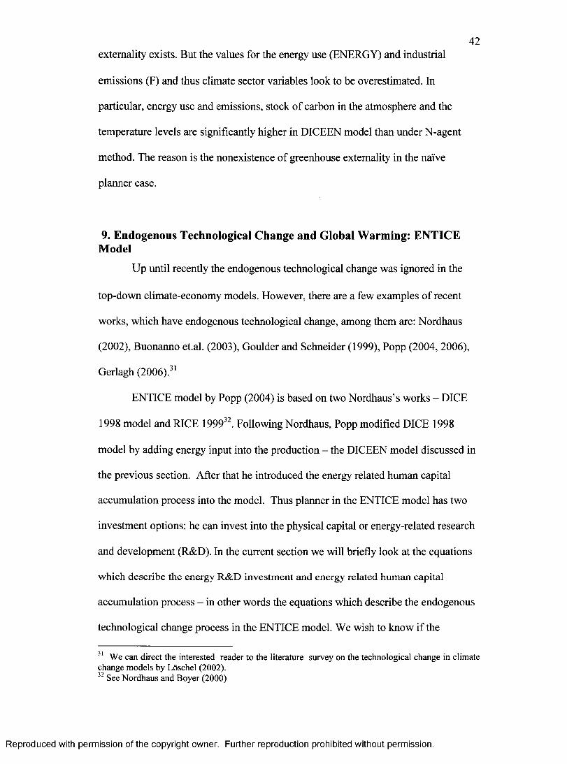
42externality exists. But the values for the energy use (ENERGY) and industrial

emissions (F) and thus climate sector variables look to be overestimated. In

particular, energy use and emissions, stock of carbon in the atmosphere and the

temperature levels are significantly higher in DICEEN model than under N-agent

method. The reason is the nonexistence of greenhouse externality in the naive

planner case.

9. Endogenous Technological Change and Global Warming: ENTICE Model

Up until recently the endogenous technological change was ignored in the

top-down climate-economy models. However, there are a few examples of recent

works, which have endogenous technological change, among them are: Nordhaus

(2002), Buonanno et.al. (2003), Goulder and Schneider (1999), Popp (2004, 2006),

Gerlagh (2006).31

ENTICE model by Popp (2004) is based on two Nordhaus’s works - DICE

1998 model and RICE 199932. Following Nordhaus, Popp modified DICE 1998

model by adding energy input into the production - the DICEEN model discussed in

the previous section. After that he introduced the energy related human capital

accumulation process into the model. Thus planner in the ENTICE model has two

investment options: he can invest into the physical capital or energy-related research

and development (R&D). In the current section we will briefly look at the equations

which describe the energy R&D investment and energy related human capital

accumulation process - in other words the equations which describe the endogenous

technological change process in the ENTICE model. We wish to know if the

31 We can direct the interested reader to the literature survey on the technological change in climate change models by Loschel (2002).32 See Nordhaus and Boyer (2000)


43introduction of endogenous technological change will affect our results obtained

before.

Modeling the endogenous technological change begins with describing the

human capital accumulation process33:

Ht+1 - H t = h (R Et) - 5 HH, (9.1)

where Ht is the energy related human capital, RE t is the energy related R&D

investment and h(RE t) is the innovation possibility frontier, the rate 5H is the rate

of decay of energy related knowledge. Popp assumes the following functional form

for the innovation possibility frontier:

h(RE,) = aR‘ ,H*E, (9.2)

and argues that the empirical evidence suggests diminishing returns to R&D

investment, b + <j) < 1. The next step is to modify the equation (8.2), now that the

energy input can be “produced” by means of fossil fuels and human capital. Popp

assumes them to be substitutes and the “energy production function” takes the

following form:

ENERGY, =

i /p

(9.3)

where a , and aH are the scaling factors, and p is the substitution parameter for

fossil fuels and energy related knowledge.

Since energy R&D investments are now allowed in the model, the resource

constraint of the model becomes:

33 Popp models explicitly energy related R&D investment and human capital which relates to energy efficiency. Other sectors R&D investments are modeled only implicitly.


44Yt = C t + I t + R E>t. (9.4)

Popp concludes that the effect of induced innovation is negligible and explains

that this happens to the certain extent due to inefficiencies of R&D market. This

completes the discussion of the main features of the ENTICE model and below we

will present the results of the BAU scenarios computation using approach developed

by Popp and N-agent method.

Calculation of the BAU scenario in the ENTICE model takes the same steps

as described in the previous section. In the ENTICE model the adjusted economy

sector variables are the same as in DICEEN; energy related R&D and human capital

remain unadjusted as energy input and fossil fuel use. Our version of the ENTICE

model is called ENTICE-N where the world is divided into 100 identical regions as

before. The results are similar to those obtained in the previous section. On the first

diagram we present the optimal paths of industrial emissions for the original

ENTICE model.


45

Figure 9.1: Optimal paths for ENTICE and ENTICE-N industrial em issions

m<D>.<uQ.M

CA

18

16

14

12

10

8

6

4

2

021951995 2045 2095 2145

-ENTICE — N-agent ENTICE \

As before we observe the identical curvatures of the optimal paths, however

the aggregate emissions in ENTICE-N model are lower over the time. The next

diagram presents the percentage deviation between the approaches.

Figure 9.2: Industrial Emissions and Atmospheric Temperature: Deviation of ENTICE-N from ENTICE (%)

5

4

3

2

1

0

1

2

■3

•4

521951995 21452045 2095

s9 0

■ Industrial emissions —■— Atmospheric temperature


The maximum deviation for the industrial emissions reaches 3.6% and

1.32% for the relative atmospheric temperature levels. We are also interested how

the presence of externality affects the energy R&D investment (Figure 9.3).

Figure 9.3: Energy R&D Investment: Deviation of ENTICE-N from ENTICE(%)

2

1

0

■1

2

■3

-4

■51995 2045 2095 2145 2195

On the Figure 9.3 the maximum deviation from ENTICE model reaches

3.2% in 2215. The less extensive use of fossil fuel keep its prices lower, which in

turn affects R&D investment and human capital accumulation. Also, it is reasonable

to argue that not only energy prices can drive energy related R&D (induced

innovation hypothesis), but also the climate damages experienced by the agents can

affect the amount of energy R&D investment as long as there exists the partial

internalization o f externality.

The divergence between adjusted values of the variables in ENTICE and the

corresponding variables in ENTICE-N is again insignificant (Figure 9.4).


47

Figure 9.4: Capital Stock: Deviation of ENTICE-N from ENTICE (%)

4

2

0

2

-4

■6

8

-101995 21952045 2095 2145

adjusted —■— unadjusted

Thus, under the greenhouse externality the R&D investment, fossil fuel use

and thus stock of GHG and the relative temperature level tend to be significantly

lower than in the case with naive agent modeled by Popp.34 The adjustment

procedure developed by Popp provides the values of economy sector variables

(Y,K,C,I), which are very close to those obtained using N-agent approach.

10. Conclusion

This chapter discussed a family of integrated assessment models: the seminal

DICE 1994 model by Nordhaus and its extensions. In these models a number of

scenarios were considered.

34 Appendix D contains the set o f figures describing the deviation between the results o f ENTICE and ENTICE-N models


48The business-as-usual scenario is typically used as a reference point for

comparing different policy options. It was argued that under the baseline policy the

agents did not control their emissions and the greenhouse externality existed, which

was fully internalized under the Pareto-efficient policy.35

We pointed out that there are no external pollution costs in the framework of

the DICE 1994 due to the specific feature of the model: the whole world is modeled

as single region with a single decision maker. We demonstrated that in this case the

climate damages are fully internalized even under business-as-usual scenario.

So far two methods were suggested to compute the baseline case for the

DICE and its variants. The original approach used by Nordhaus was to implicitly

assume the unavailability of the abatement technology in the baseline scenario. Popp

(2004) modeled the naive agent who does not observe the effects of global warming.

Under this way of modeling, the externality does not exist in the first place. The

resulting values for the naive agent are adjusted to the climate damages ex-post.

Both the methods do not have strong theoretical background and their attractive

simplicity of computational approach in estimating the baseline scenario may in fact

lie beyond Einstein’s famous threshold (“everything should be made a simple as

possible, but not simpler”).

Our goal in this chapter was to develop the method of modeling the business-

as-usual scenario, building on the theoretical base for the DICE class models where

the greenhouse externality comes into play. In this development we used the concept

of Open Loop Nash Equilibrium (OLNE). In particular, we divided the world into a

large number of identical regions and assumed non-cooperative behaviour. By

means of a simple analytical model we demonstrated that when the amount of

35 Nordhaus (1994) p.79


49regions becomes arbitrarily large, the climate externality exists and is not

internalized. This approach may be termed the N-agent approach.

Our theoretical predictions suggest that under the N-agent approach the

world aggregate emissions are higher than in the case when the climate damages are

internalized (Nordhaus’ approach). We also compared the results of OLNE to the

case when the naive agent is not aware of the global warming. In this case the

emissions of the naive agent are higher than the aggregate emissions of N agents.

Our empirical findings confirmed the hypotheses. We began with the original

DICE 1994 model. We found that the world aggregate pollution under the N-agent

approach is higher than in the original baseline scenario of DICE 1994. The

difference between these base estimates is not substantial due to the limited number

of variables under control of the agents and their limited effectiveness - the

maximum deviation between the optimal paths was 0.67%, but it the long run

equilibrium it was about 1 %.

Our next step was to examine the effectiveness of another approach to the

baseline computation modeling suggested by Popp (2004). We first looked at his

DICEEN model where the energy input was added to the production function. In this

case the agents could choose the level of the energy use and thus emissions level

directly, and become more flexible in reacting to the externality. We found out that

his approach overestimates values for the energy input use, industrial emissions and,

as a consequence, all the climate sector variables relatively to the values obtained

through the N-agent approach. In particular, the peak difference for the volume of

industrial emissions reaches 3.4% and is expected to grow over longer time horizons.

Note also that Popp’s final values after applying the ex-post adjustment are very


50close to ours, thus indicating that the N-agent approach can yield satisfactory

empirical results without sacrificing the theory.

Similar results were obtained for the ENTICE model in Popp (2004), which

is based on DICE 1998 but characterized by the endogenous technological change.

We found out that in the presence of externality, the driving factors of this

technological change (energy R&D investment and the energy human capital stock)

are lower than in the case when externality does not exist. Industrial emissions - and

therefore the related climate sector indicators - are also smaller. Just as for the

DICEEN model, the difference between the values of the adjusted variables and the

corresponding variables obtained under the N-agent method is marginal.

Thus we demonstrated the advantages of given approach, which is built on

the theoretical background and can be easily used in the empirical models. This

approach can be advantageously applied to studying other global models of the

world with externalities (negative or positive).


51References

Basar T., Olsder G., 1982. Dynamic Non-cooperative Game Theory. Academic Press. London, New York.

Buonanno P., Carraro C., Galeotti M., 2003. Endogenous Induced Technical Change and the Costs of Kyoto. Resources and Energy Economics 25 (1), pp. 11-34.

Bromley D., 1993. Environment and Economy. Blackwell, Cambridge USA.

Gerlagh R. and Lise W., 2005 Carbon Taxes: A Drop in the Ocean, or a Drop that Erodes the Stone? The effect of Carbon Taxes on Technological Change. Ecological Economics 54. pp.241- 260

Gerlagh R., 2006. A Climate Change Policy Induced Shift from Innovations in Carbon Energy Production to Carbon Energy Savings. Energy Economics, forthcoming

Goulder L., Schneider S., 1999. Induced Technological Change and the Attractiveness of C02 Emissions Abatement. Resources and Energy Economics 21 (3-4), pp. 211-253.

Jaffe A., 1986. Technological Opportunity and Spillover of R&D Evidence from Firms’ Patents, Profits, and Market Value. American Economic Review 76 (5), pp.984-1001.

Lewis K., Seidman L., 1996. An Optimal Greenhouse Tax in an Optimal Growth Model.Southem Economic Journal 63(2), pp. 418-28.

Loschel A., 2002. Technological Change in Economic Models of Environmental Policy: A Survey. Ecological Economics 43 (2-3), pp. 105-26.

Mansfield E., 1977. Social and Private Rates of Return from Industrial Innovations. Quarterly Journal of Economics 91 (2), pp. 221-240.

Mastrandrea M., Schneider S., 2004. Probabilistic Integrated Assessment of “Dangerous” Climate Change. Science 304 (5670), pp. 571-575.

Nordhaus W., 1976. Economic Growth and Climate: Carbon Dioxide Problem. Cowles foundation Discussion Paper 443.

Nordhaus W., 1994. Managing the Global Commons: The Economics of Climate Change. MIT Press, Cambridge, MA.

Nordhaus W., 2002. Modeling Induced Innovation in Climate-Change Policy. Technological Change and the Environment, edited by Griibler A. et al. Resources for the Future, Washington, DC, pp. 182-209.


52Nordhaus W.,Yang Z., 1996. A Regional dynamic General-Equilibrium Model of Alternative Climate-Change Strategies. American Economic Review 86(4), pp741- 765.

Nordhaus W., Popp D. 1997. What Is the Value of Scientific Knowledge? An Application to Global Warming Using the PRICE Model. Energy Journal, 18(1), pp. 1-45

Nordhaus W., Boyer J., 2000. Warming the world: Economic Models of Global Warming. MIT Press, Cambridge, MA.

Pigou A., 1920. The Economics of Welfare. London, Macmillan.

Popp D., 2004. ENTICE: Endogenous Technological Change in the DICE Model of Global Warming. Journal of Environmental Economics and Management 48, pp. 742-768.

Popp D., 2006. ENTICE-BR: The Effects of Backstop Technology R&D on Climate Policy Models. Energy Economics, 28(2), pp. 188-222.

Shiell L., 2003. Descriptive, Prescriptive and Second-Best Approaches to the Control of Global Greenhouse Gas Emissions. Journal of Public Economics 87, pp. 1431-1452.

Smith A., 1950. Wealth of Nations. New York, Dutton.

Woodward R., Bishop R., 1997. How to Decide When Experts Disagree: Uncertainty-Based Choice Rules in Environmental Policy Land Economics 73(4), pp. 492-507.

Xepapadeas A., 1997. Advanced Principles in Environmental Policy. Edward Elgar, MA.


Appendix A. Structure of the DICE 1994 Model

Exogenous variables

<Tt - rate of decarbanization: ratio of GHG emissions to output

At - total factor productivity

Lt - population of the world, equal to the labour force

g° - growth rate of <Jt

gtL - growth rate of Lt

g,A - growth rate of At

FORCOTH, - forcing of exogenous GHG

Endogenous variables:

Ct - consumption

Yt - net output

Kt - capital stock

It - gross investment

Et - GHG emissions (CO2 and CFCs) million tons of CO2

Mt - mass of GHG in the atmosphere

Ft - radiative forcing from GHGs

TEt - change in global mean atmospheric temperature since 1865

TLt - change in mean deep-ocean temperature since the base period

Dt - damage from greenhouse warming

Qt - output scaling factor due to emissions controls and to damages from

climate change

TCt - total cost of reducing GHG emissions


Policy variables:

I, - gross investment

p t - rate of emissions reduction

Parameters

5k - rate if depreciation of the capital stock

8 m - rate of transfer of GHGs from atmosphere to deep ocean

b, ,b2 - parameters of emissions-reduction cost function

P - elasticity of output with respect to capital

a - marginal atmospheric retention rate

X feedback parameter in climate model

C, ,C2 ,C3 - thermal coefficients

0 ,,0 2 - damage function parameters

p - rate of social time preference

Economy sector

K t+1=It+ ( l -8 K)K t

Y = Q tA tKPLVP

Yt=Ct+It

Et=(l'M-t)crtAtKpL1t'p

Climate sector

Mt+1—Mt =aE t —Sm(M ,-590)

FORC, =4.1 log /log2+FORCOTHt

TEt+] -T E t = C^FORC, -X TEt - C 3(TEt - TLt))

TLt+i - TLt = C4 (TEt - TLt)


Climate feedbacks

D,=l+e,TEf‘

T C .-bj^A .K fl*

n

D,


Appendix B. Steady State for DICE 199456

In this appendix we derive the equations in order to calculate the steady state of the

• • • 36DICE 1994 baseline scenario, emissions control rate p is set to zero.

Constraints of the model:

K(t +1) - K(t) = 10[I(t) - 8 KK(t)] (Bl)

E(t) = 1 Oa(t)A(t)L(t)1_p K(t)p (B2)

FORC(t) = 4.1* log(M(t) / 590) / log 2 + FORCOTH(t) (B3)

M(t +1) - M(t) = aE(t) - SM (M(T) - 590) (B4)

TE(t +1) - TE(t) = Cl[FORC(t) - (X + C3)TE(t) + C3TL(t)] (B5)

TL(t +1) - TL(t) = C4[TE(t) - TL(t)] (B6 )

Y ( t)= A(t)L(ty-pK(t)p (B7)

(1 + — TE(t)2)

C(t) = Y (t)-I( t) (B8 )

Each period t in the present model equals to ten years, but the values for the rate of

time preference, capital depreciation are in their annual terms, so they must be

multiplied by the factor 1 0 .

Combining equations (B1),(B7),(B8):

K(t +1) — K(t) = AfflLW 1 PK(t)p _ C(t) _ w t ) (B9)

(1 + — TE(t)2)

(B2),(B4) together:

M(t +1) - M(t) = a l 0a(t)A(t)L(t),“p K(t)p - 8 M (M(T) - 590) (B10)

36 Also note that some parameters take their specific forms used in the DICE 1994, for example theAl

damage function parameters are now equal: 0, = --- ,0 2 = 2 .


57(B3),(B5) together:

TE(t +1) - TE(t) = Cl[4.1 log(MAT(t) / 596.4) / log(2) + +FORCOTH(t) - (k + C3)TE(t) + C3TL(t)]

( B 11)

The planner maximizes the inter-temporal utility function:

subject to:

(B9 ),(B1 0 ),(B1 1),(B6), transversality conditions and the initial values for K, M, TE, TL.

In this problem there is one control variable: C. The state variables are: K, M, TE, TL and

the corresponding co-state variables are: pK, pM, pTE, pTL

In order to solve the maximization problem we employ the optimal control theory and write

down the current-value Hamiltonian:

+p(t)M [a l Oa(t)A(t)L(t)'-pK(t)p - 8 M (M(T) - 590)] +

+p(t)TE [Cl[4.1 * log(M(t) / 590) / log(2) + FORCOTH(t) - (k + C3)TE(t) + C3TL(t)]] +

+P(t)TL [C4[TE(t) - TL(t)]]

= pK -10pp(t)K = -10p(t)K [pY (t)/ K (t)- 8 K] - p(t)MPE(t)/ K(t) (B13)

+ioP(t)K A^ LAf PK^>P(1 + — TE(t)2)

- C ( t ) - 5 KK(t) +

The first order conditions:

(B12)

— =pM-10ppM=p(t)M5M-p(t)TE(4.1*Cl)/(log(2)*M(t)) 5M

(B14)


58A1

3H 2 — TE(t)Y(t)OTT3- = P -1 Opp(t) —p(t) — ----------- + p(t) (A + C3)C1 - p(t) C4OTE (l + f T E ( t ) J)

(B15)

= pTL - 1 Opp(t)TL = -p (t)TE C3C1 + p(t)TL C4 (B16)d T L

In the steady state pK = pMAT = pTE = pTL = 0, therefore we rearrange the first-order

conditions (B13)-(B16)37:

10pK[p Y /K -8 K-p ] = - p MpE/K (B13’)

PM (SM+1 Op)=pTE (4.1 *C 1 )/(log(2)*M) (B14’)

A1Y (2^~TE)

pTE ((X + C3)C1 +10p)=pTLC4 - 1 0pK ------- (B15 ’)(1 + — TE2)

9

pTL(C4+10p) = pTEC3Cl (B16’)

Also in the steady state K = MAT = f E = TL = 0 , hence the constraints of the

model (equations (B9)-(B11) and (B6 )) become:

I = 8 kK (B17)

aE = 8m(M -590) (B18)

FORC = (A, + C3)TE - C3TL (B19)

TE = TL (B20)

For the numerical calculations of the steady state the following equations are used:

(B2),(B3),(B7),(B8) in their steady state and (B12),(B13,)-(B16’),(B17)-(B20).

37 The variables and parameters without the time reference denote the steady-state value o f a variable or a parameter.


59However, we also need the steady state values for all exogenous parameters such

as labour(L), technological change(A), rate of decarbonization( o ), exogenous

forcing of other GHG (forcoth).We calculated the following steady state values for

these parameters:

limA(t) = 0.038 limL(t) = 10571.965, limo(t) = 0.179, limFORCOTH(t) = 1.420t —>oo t —>oo t —>oo t —>oo

To get the numerical solution the GAMS software was used and the results are

presented in the Table 7.1.


Appendix C. Deviation from DICEEN Model

Figure 1C: Consumption: Deviation of DICEEN-N from DICEEN (%).

-101995 2045 2095 2145 2195

unadjusted —■ —adjusted


61

Figure 2C: Output: Deviation o f DICEEN-N from DICEEN (%)

-10 J1995 2045 2095 21952145

-unadjusted —■— adjusted


62Appendix D. Deviation from ENTICE.

Figure 1D: Output: Deviation o f ENTICE-N from ENTICE (%)

-101995 2045 2095 2145 2195

Adjusted Nonadjusted


63

Figure 2D: Consum ption: Deviation o f ENTICE-N from ENTICE (%)

-101995 2045 2095 2145 2195

■adjusted —■—unadjusted


64

Figure 3D: Human capital: Deviation of ENTICE-N from ENTICE (%)

0.4

0.2

0

- 0.2

-0.4

- 0.6

- 0.8

1

- 1.21995 2045 2095 2145 2195


65

Figure 4D: GHG stock in the Atm osphere : Deviation o f ENTICE-Nfrom ENTICE (%)

0.5

0

-0.5

1

1.5

■221952095 214520451995


Chapter 3A Perspective on Scarcity Debate in the Context of the

Climate Change Problem

1. Introduction

Forster (1980) is credited with being the first researcher to combine the ideas

of the natural resources economics to those of the environmental economics in the

context of the optimal growth model. Moreover, the Forster’s work contributed by

discussing the energy-environment trade-off. In the following years the idea of

mixing the features of resource and environmental economics in the climate change

models was often used by researchers. Thus the questions of the optimal resource

depletion and the pollution externality are now examined simultaneously (Farzin

(1996), Tahvonen (1997), Hoel and Kvemdokk (1996)).

It is straightforward to show that the gross price of the polluting non

renewable resource in the first-best world includes the resource and pollution

shadow prices. In contrast, in deriving the decentralized market equilibrium one can

demonstrate that private agents might ignore the social prices of pollution and

resource stocks. Therefore, the optimal tax program that would make the

decentralized solution identical to the socially efficient one must include the shadow

values of both stocks.

It is known that shadow values are sensitive to the various parameters of

the model, such as rate of time preference, pollution stock decay rate etc. It might be

the case that under a certain set of assumptions the resource stock shadow value is

negligible and therefore does not affect the size of the optimal tax significantly.

Thus, one can conclude that the environmental considerations prevail over the

66


67concern about the fuels scarcity. Alternatively, the share of the pollution shadow

price might be insignificant relatively to the scarcity rent, meaning that the society is

focused on the scarcity issues, ignoring the pollution cost.

Although the formal analysis of whether the environmental considerations

are prevailing over the issues of scarcity has not yet been performed in the context of

the global warming issue, the role of the scarce fossil fuels in the climate change

policies is being widely discussed. There are two polar opinions: the first is that the

supply of fuels is virtually unlimited and it is a matter of technological progress to

maintain the era of cheap fuels indefinitely (Martin (1999)). Therefore the policy

makers have to rely on carbon taxes to achieve the desired environmental targets and

prevent the possible catastrophic events caused by growing mean temperature level.

The second opinion argues that the world is about to run out of conventional fuels,

which means that the climate change policies should not get the priority in the

world’s agenda (Campbell and Laherre (1998)).

The most recent estimate of the fossil energy deposits can be found in IPCC

2001 report. The report indicates that there are approximately 200 billion metric tons

of carbon (GtC) of proven conventional oil and gas reserves and approximately

1.000 GtC of coal. Also there is an estimate of another 300 GtC of unconventional

oil and gas deposits, making the fossil energy reserves to be around 1,500 GtC. The

whole resource base (which includes reserves and resources) is estimated to be about

5.000 GtC .38

1 Rogner (1997) defines these terms as follows: “Reserves are those occurrences that are identified, measured, and at the same time known to be technically and economically recoverable” and “Resources are occurrences with less-certain geological assurance and/or with doubtful economic feasibility.” The resource base is the sum o f reserves and resources. For detailed discussion, see Rogner (1997), pp.219-222.


6 8The most abundant fossil fuel is coal and its share in reserves and

resources of fossil is about 70%. Most researchers agree that, regardless of the

abundance of coal deposits, it is highly unlikely that the world will rely on coal,

especially if the environmental damages caused by burning coal are internalized,

since the carbon content of coal is very high. Moreover, most of the coal reserves are

considered uneconomic. As Grubb (2001) points out, in order to reach the

stabilization target of 450ppm C 0 2 the world will have to emit another 620-650

GtC, which is significantly higher than the amount of proven conventional oil and

gas reserves. Does that imply that the climate change problem is irrelevant? In

fact, Grubb argues that: “The longer-term problem of climate change arises from the

fuller and longer-term use of coal, and of unconventional carbon deposits such as

heavy oils, tar sands and oil shales”.

However, in his recent book Tertzakian (2006) writes: “There are two angles

to the “are we running out of oil” debate: the intuitive angle is that we are indeed

running out of reserves, but that is simply not the case. There are billions of barrels

of oil reserves remaining on the planet. The real issue is that we are running out of

reserves that provide enough economic incentive to produce with today’s technology

and in our current geopolitical atmosphere”. Thus one might want to know how

much of fuels could be eventually extracted given the today’s technology and what

kind of effect it might have on the global warming and the welfare of the future

generations. The model used in the present chapter allows to answer these questions.

The objective of the chapter is to consider the trade-off between the scarcity

rent and pollution cost in context of climate change problem and to evaluate the

39 For the details see IPCC (2001) and Grubb (2001).


69trade-off quantitatively. As the indicator of the trade-off we choose the ratio of the

resource and pollution shadow prices. We wish to identify the conditions under

which the scarcity considerations dominate the environmental ones. This issue has

not been much discussed since Forster (1980) considered the pollution-energy trade

off using a simple optimal growth model. We are aiming to define and find the

“true” resource and pollution shadow prices relationship (ratio) in the model that is

characterized by perfect certainty, presence of the central planner and the equitable

treatment of all generations. We present the numerical simulations that allow us to

provide the quantitative assessment of the trade-off. Seeking the answer to this

question there arise particular methodological issues, such as the finding the optimal

time horizon of the model, avoiding the “repugnant conclusion” etc. The chapter also

to the certain extent contributes to literature on the cake-eating problem with zero

rate of time preference originated by Gale (1967) and Koopmans (1973) by

developing empirical estimates of the optimal time horizon.

We first start with constructing the analytical model and discuss the relevant

theoretical and methodological issues. After that armed with theoretical findings and

methods, we employ the integrated assessment model (DICEEN) which is based on

the ENTICE model due to Popp (2004), modify it according to our purposes and

perform the numerical simulations to answer the question of pollution-scarcity

relationship.

2. The Model

In some of the models of environment-economy interactions, emissions are

modeled mostly as the by-product of the output production (Forster (1972),d’Arge

and Kogiku (1973), Falk and Mendelsohn (1993), Tahvonen and Kuuluvainen


70(1993), Nordhaus (1994)). This assumption significantly simplifies the structure

of the model. However, an important feature of the problem is ignored: the

extraction paths of fossil fuels are neglected in those models. In the pioneering work

by Forster (1980) it was shown how to combine the ideas of resource and

environmental economics in the context of the optimal growth model. Due to

Forster’s contribution the researchers began to introduce the fossil fuel stock in their

models (Farzin (1996), Hoel and Kvemdokk (1996), Nordhaus and Boyer (2000)),

Chakravorty et al. (2006). In some of the models of this class the stock of the fuels is

assumed to be known and fixed (Nordhaus and Boyer (2000), meaning that research

relies on the physical scarcity of the resource. In contrast, some models assumed

economic scarcity, which implies that although the fuels are non-renewable, they are

not exhaustible (Hoel and Kvemdokk (1996), Farzin (1996)).

2.1. Centrally Planned Economy

In this section we build a simple analytical model with two stocks in

question: pollution and resource and discuss the theoretical issues that are relevant in

the long-term analysis of scarcity and pollution.

In the model the world is treated as one region. There is a central planner

who makes the production-consumption decisions. The world economy produces a

single good. The output at time t ( Yt ) is produced by means of capital ( Kt ),

e n erg y /fo ss il fu e ls ( F, ) and labour ( L , ): Q (K t, F t , L ,) ,40 In the m o d e l labour is

assumed to be exogenous. We assume that the production function is strictly

concave, twice differentiable and exhibits constant returns to scale:

40 In the theoretical model we assume that one unit o f fossil fuels provides a unit o f energy, thus we ignore the possibility o f carbon-saving technical change over time. Such technological change will be introduced in the empirical simulations.


71Qx > 0,QXX < 0 where x = K,F 41 We also assume that the inputs are essential:

Q(0, F, L) = 0 and Q(K, 0, L) = 0 . The world is endowed with some initial capital

stock ( K0).

The use of energy input generates a stock of greenhouse gases (St), which

accumulate in the atmosphere according to the following law of motion42:

S = F - 8 sS, (1)

where 8 S is the decay rate of the pollution stock.43 The stock of greenhouse gases

(S) negatively affects the output production via increased atmospheric temperature

levels. Thus we introduce the damage function D(S) which possesses the following

properties: D(0) = 1, D' < 0, D" < 0 . The output adjusted to climate damages is

given by: D(S)Q(K,F,L).

In each period some amount of fuels is extracted, building the stock of

cumulative extraction Cm, according to the relationship:

Cm = F (2)

The total fuel extraction costs at time t is the product of the current extraction ( F,)

and the unit extraction cost Z(^ m* ) ,i.e. )Ft , where Cm* is the positiveCm Cm

“extraction limit” parameter, that will be discussed below. The unit extraction cost is

41 To denote the partial derivative o f function F with respect to x the following notation is used: Fx42 In what follows, the terms “the stock o f greenhouses gases” and “the carbon stock” are interchangeable.43 The notation F denotes the time derivative.


72assumed to be the strictly convex function of cumulative extraction:

Z( r) > 0 VCm,, Z '> 0 , Z "> 0 .Cm

The “extraction limit” Cm* can be interpreted as a “hard” limit in a

Hotelling’s sense. We can assume that Cm’ is the maximum amount of the

extractable fossil fuels and impose the constraint: Cm, < Cm*, V t. In this case we

have the usual Hotelling model with fixed and known stock of the resource. In this

case the physical scarcity is assumed.44

Alternatively, it can be treated as a “soft” limit. The cumulative extraction

Cm, can go beyond Cm* at the corresponding high costs. In this case the parameter

Cm* indicates the convexity of the cost function and can be also called as the “cost

function convexity parameter”. The stock of fuels in carbon units is assumed to be

unlimited, meaning that a model relies on the economic scarcity rather than on the

physical one.45

At each period t the planner distributes the output between the capital

investment, K , consumption, C, and fossil fuel expenditures, i.e.

K = D(S)Q(K, F, L) - C - Z ( - ^ ) F - 5kK (3)Cm

where 8 k is the decay rate of capital stock. The central planner wishes to maximize

00 Q

an aggregate welfare function V = |LU (—)e“ptdt where L denotes the population of0 L

44 The similar cost function was assumed in Nordhaus and Boyer (2000). In their case only the

physical scarcity was considered,, i.e. the constraint Cm, < Cm , Vt was in place.

45 In what follows, the terms: “convexity parameter” and “soft limit” mean that the constraint

Cm, < Cm , Vt does not hold. In the analytical model we assume the “soft” limit.


73C

the world (assumed equal to labour force), — is the per-capita consumption, U(-)L

is the strictly concave utility function and p is the rate of time preference.

To solve the planner’s problem the optimal control theory can be applied.

The planner’s control variables are the aggregate consumption (C) and energy

use/extraction (F), and the state variables are the capital stock (K), the pollution

stock (S) and the stock of cumulative extraction ( Cm ). The current-value

Hamiltonian of the problem is written as:

H=LU(^)+?i D (S)Q(K,F,L)-C-Z(-^)F-5kKCm

+p[F-8sS]+0F

where co-state variables k , p and 0 represent the shadow values of capital,

pollution and the resource stock respectively.

Assuming the existence of the interior solution, the first-order conditions of

the planner’s problem are the following (where the superscript “P” denotes the

solution values of the planner’s problem):

dC LU'(— ) - k p =0 (4)

* U p5F

D(SP )QF(KF ,FP ,L)-Z( r )Cm

+pp+0P=O (5)

~ = V - p V = -Xp[D(Sp)Qk(Kp,Fp,L ) - 5 k] (6)SK

~ = 1ip-ppp=(1p5,-X.pD'(Sp)Q(Kp,F p,L) (7)

5H - e p -Pep =xpz'(^!5L) T L (8)3Cm Cm Cm

and the equations (l)-(3) and the standard transversality conditions.


74In our further analysis we will need the expressions for the pollution and

resource shadow prices. In order to obtain the shadow value of the pollution stock

we first need to integrate (6 ) and (7):

v

- J(8K+ p - D ( S P ( q ) ) Q K ( K P ( q ) , F P ( q ) , L ( q ) ) ) d q

A.p(t) = A,p(v)e ‘ , v > t (9)

oo

p p( t)= Jexp"<Ss+p)<v",) V (v )D '(S p(v))Q (K p(v ),F p(v),L (v))dv (10)t

Substituting (9) into (1 0 ) for A,P(v) we derive the expression that describes the

pollution stock shadow price:

v

- J ( 8 s + D ( S p ( q ) ) Q K ( K p ( q ) , F p ( q ) , L ( q ) ) - 8 K )d q

p p(t) = V(t)Jexp ■ D'(Sp(v))Q (K p(v ),F p(v),L (v))dv

This equation is the discounted sum of the values of the marginal damages, which

happen due to the increase in the carbon stock by one unit at time t. This shadow

price of pollution can also be considered as the discounted marginal benefits if the

additional unit of emission is not emitted at t.

Integrating (8 ) and substituting (9) we obtain the resource stock shadow

price:

v

°° [_ ( d ( S p ) Q k ( K p , F p , L ) - 6 k ) d q

e p(t) = -? ip(t)Je- Z'( Cm p(v )N|F p(v)

-dv (12)Cm

The equation gives the present value of the increase in the costs of extraction over all

future periods due to the extraction of one unit of fuels at time t which means that

extracting one unit of fuels at t increases the extraction costs over the remaining

periods of the planning horizon of the model.


75In what follows we will also need the equilibrium condition of resource

extraction. Rearranging (5) we obtain:

It can be seen from (4), (11) and (12) that A,p>0, fip<0 and 0P < 0. Hence equation

(5') suggests that the gross price of the resource - i.e. the value of the marginal

product of the additional unit of fuels - must be equal to the value of extraction costs

plus pollution and resource shadow prices. Also note that equation (5') gives the

implicit demand function for energy. Since A,p>0, pp<0 and 0P < 0 , the

equation (5') also implies:

Thus in this section we have solved the problem of the central planner and

derived the social shadow prices of the resource and pollution stocks: (1 1 ) and ( 1 2 ).

We have also described the socially optimal price of fuels that consists of three

elements: unit extraction cost, social shadow prices of the pollution and resource

stocks as shown in (5').

2.2. Decentralized Market System. Optimal Tax

Obviously those values of the shadow prices of resource and pollution

derived above would be different in the case of the decentralized equilibrium due to

the presence of externalities. Therefore we have to derive the decentralized

(S')

D(Sp)QF(Kp,Fp,L ) > Z ( f l C )Cm

(13)


76equilibrium and compare it to the planner’s solution so as to obtain the optimal tax

program that would internalize the externalities.

In the model discussed above the world was represented by single region. In

order to calculate the decentralized equilibrium in single region model of the world

we have to use the N-agent approach developed in Chapter 2. Following the

approach we have to divide the world into the N identical regions. Each of regions

has its own planning agent who makes consumption-production decisions for his

portion of the world economy. The production side is identical to the one discussed

in the planner’s problem described above.

In the model we consider the case of market imperfections when the owners

of the resource fail to charge the user cost of the resource. Alternatively, private

resource owners may impute a different user cost to the resource than the social

planner, owing to a different rate of time preference or particular features of their

tenure. For simplicity, we have modeled the extreme case of failure by private agents

to charge any user cost, which is formally equivalent to open access.46

Thus we assume that agents behave non-cooperatively and each agent i,

i = 1,..,N considers the extraction efforts and emissions of other N-l agents as

given 47 Thus:

46 Interestingly that in the dynamic computable RICE 99 model Nordhaus and Boyer (2000) are not entirely clear on their assumptions regarding the fossil fuels market and one possible way of interpretation the equations o f the RICE99 model that describe the fuels market is that it ischaracterized by the open access.47 In what follows, the upper-case letters denote the economy aggregate values and the lower-case

N N

denotes the agent’s specific: ^ C, t = C t /, t = L t .i=l i=l


77

M + £ f j - 8 sS (14)j*i

and

J * i

in

where ^ f j represents the exogenous emissions/extractions of other N-l agents.

Each agent is endowed with the N-th portion of the world’s capital stock:

K Lkj 0 = and have identical labour supply - the population of region: /, = — . In

each period of time the agent allocates the output between consumption, capital

investment and the purchase of fuels expenditure:

k = D(S)q(k,f,/)-c-| Z ( - ^ - ) + t W k + T (16)V Cm )

where x denotes the externality tax on the fuel input and T is the lump sum transfer

of the tax revenue. These values are exogenous to the agent. We assume that all

agents receive back their tax payments in the form of the lump-sum transfer T=xf to

maintain the balanced government budget.

ca ^Each agent i maximizes the inter-temporal utility function V = j7(J(—)e ptdt

o ^

c C /N(where — = is the per-capita consumption) subject to the constraints o f the

model (14),(15),(16) and the transversality conditions. The solution to the game is

characterized by the Open-Loop Nash equilibrium given the assumption of the


78perfect foresight. The current-value Hamiltonian of the agent’s i problem is the

following:

H=/U(y)+Z( Cm i N —

D(S)q(k,f,/)-c- Z(— - ) + Tv c m )

+0IN

f + 2 Tj*>

where co-state variables X , p and 0 represent the shadow values of capital,

pollution stock and the resource stock respectively.


the agent’s problem are the following (the superscript “NE” denotes the Nash

Equilibrium values of the variables):

py /-»NE

— =u'(— y x m =o3c /

(17)

3f■ = X* D(SNE) q f ( k ^ T ^ , / ) Cm

z ( o i r )+T

3H 3k^ =1NE -pX™ =-X™ [D ^ 1® )qk (k ^ ,f1NE ,l)-8 k ]

3H3S

* N E , , N E , , N E £ ^ N E t V / c N E 'v r t / u N E j?N E i \- p -pp - p os-A, D (S )q(k ,f ,1)

3H •3Cm

NE x 'N E a N E _ q N E 'v NE 7 / / v - 'I I l 1-0 -p0 - x z ( t

Cm Cm

+pNt+0Nt=O (18)

(19)

(20)

(21)

equations (14)-(16) and the transversality conditions. Rearranging (18) we obtain the

equilibrium condition for fuels extraction of the agent i:

D(SNE) q f ( k ^ ^ ^ , / )CmNE „ ^ p ^ 0*®Cm NE 0 NEX™ X

(22)

Our objective is to derive the optimal tax program x that would make the

decentralized equilibrium identical to the socially optimal. In order to do this we


79have to find the solutions for the shadow values of the resource and pollution

stocks. Integrating (19) we obtain the shadow value of the capital stock:

- f ( 8 K + p - D ( S NE( q ) ) q k ( k NE( q ) , f NE( q ) , l ( q ) ) ) d q

A,NE(t) = A,NE(v)e * , v > t (23)

Solving for p in (20) we have:

oo

p NE(t) = jex p “(8s+pXv”t) ?iNE(v)D '(SNE(v))q (kNE(v ) ,fNE(v),l(v))dv (24)

Using the property of linearly homogenous functions, in particular the fact that

OfK F L)q (k ,f ,l) = — and qk = Q K and substituting (23) into (24) we obtain the

Nash Equilibrium shadow price of the pollution stock:

0 , N E / . n <*> - f ( 8 s + D ( S NE( q ) ) Q K ( K NE( q ) , F NE( q ) , L ( q ) ) - 6 K )d q

p^E(t) = — fexp * D'(Sne ) Q (K ne ( v ) , F ne ( v ) , L ( v ) ) d v ( 2 5 )N i

Equation (25) suggests that the private shadow value of the pollution stock is the —N

of the total discounted sum of the values of the marginal damages caused by the

additional unit of carbon emitted by some agent i. In other words, it says that each

agent internalizes only the self-inflicted damages. As N becomes arbitrarily large, no

internalization of damages will take place: lim (i (t) = 0 and the pollution costN - » o o

becomes fully external.

The resource shadow value can be obtained by integrating (21), substituting

(23) and using the fact that f ; =pNE

N


If the externality tax x replicates the first-best optimum then from (4) and (17) we

see that A,NE(t) = A,P(t) . Comparing (26) and (12) we observe that:

0NE(t ) = ® J 2 (27)N

Moreover, comparing (25) and (11) we have:

NE( , ) = / ( t ) ( 2 g )

N

Rewriting (22) using (27) and (28) we obtain the gross price of the resource in the

decentralized market system ( PNE) in terms of planner’s shadow prices:

/ - i „ N E P n PpNE C r n ^ — e _ + i

Cm XPN A. N

At the same time the gross price in the first best world is given by:

*P . . P f \PCm u 0Pp=Z(----- r ) - ^ r — - as shown in (5'). Therefore the optimal tax can be evaluatedCm X X

which would make the resource prices identical in the market and socially optimal

solutions: PNE = Pp . Thus we are looking for a dynamic tax rate x such that

P ^ = P p i.e.:

m Cmp pp 0P Cmp gp 0P PF ^ "TpTt ^ r '"vP "Tp" “ ” ^Cm X N X N Cm A, X

Thus it follows from (29) that the prices are equal only if

<N-1)N

V + e Mi p\ /

(30)


81The optimal tax rate consists of the two elements: resource and pollution

shadow prices.48 Unfortunately, using the theoretical model we cannot observe the

relative size of the shadow prices along the optimal path; in other words it is not

clear if the pollution shadow price dominates the resource one or vice versa.

Therefore it is not clear if the environmental issues prevail over the scarcity

considerations. The empirical model investigates these questions further.

3. Trade-off Between Scarcity and Pollution Cost. Preliminary Empirical

Insight

As shown in equation (30) above, the optimal tax, under open-access

resources, consists of two components: resource and pollution shadow prices. From

equations ( 1 1 ) and ( 1 2 ) the factors that are likely to affect the size of these values

can be observed.

Firstly, the stock of the resource or alternatively the convexity parameter

Cm* affects the value of the resource shadow price. The higher the value of this

parameter, the lower is the scarcity rent (this can be seen from equation (1 2 )), and

therefore the optimal price of the fuels. Reducing the price of the fuels stimulates

more extensive use of the fuels, which increases society’s pollution cost: the increase

in the extraction/emission rate increases the carbon stock which in turn leads to an

48 It is not difficult to show that if the resource is privately owned, i.e. each agent is endowed with his/her own amount o f the resource, the social and private shadow values o f the resource are identical, which implies that in this case the tax consists o f one element: pollution stock shadow value.However, what is more important, the correct price o f fuels must be the sum o f three elements: unit extraction cost, resource and pollution stocks social shadow values.


82increase in the value of marginal damages D'(S) and therefore in the value of the

pollution stock shadow price.49

A factor that exclusively affects the value of the pollution stock shadow price

is the rate of its decay. The higher is the rate, the faster the carbon stock is reduced

naturally and therefore the damages from marginal unit of emissions have lower

affect. Thus the higher the rate of decay is the lower is the value of the pollution

stock shadow price.

One factor, which deserves significant attention, is the time horizon of the

model. The analytical model presented here assumes an infinite horizon but

numerical simulation model must assume a finite horizon. The change in the time

horizon of the model affects both shadow prices. We can see from equation (11) and

( 1 2 ) that the stream of marginal pollution damages in the pollution stock shadow

price is discounted more heavily than the stream of effects on extraction costs in the

resource stock shadow price by the value of the decay parameter 8 S. Therefore, the

extension of the planning horizon in a numerical model should have a greater effect

on resource shadow price than on the pollution shadow price.

Also, it is a well-known fact that both shadow prices are sensitive to the

changes in the rate of time preference: the reduction in the rate increases the

pollution cost as well as the resource rent as future values are discounted less.

Although the rate of the time preference does not show up in equations (11) and (12)

its effect comes indirectly through the marginal product of capital. Using equations

(4) and (6 ) the following well-known expression can be derived:

49 In absolute value, since D,(SP’NE ), pP,NE <0


83Q

D(S)Qk (Kt ,Ft ,Lt )-8 k =p+a— where a is the elasticity of marginal utility withct

respect to consumption. Thus the change in the rate of time preference p affects the

marginal product of capital D(S)Qk(K t,Ft,L t) , which in turn affects the discount

rate of the resource and pollution stocks shadow values.

We have identified that time horizon of the model, convexity parameter of

the cost function and rate of time preference are important factors that affect the

values of the shadow prices. However it is not clear from the analytical model the

extent to which shadow price are sensitive to the changes in the parameters than the

other.

To investigate this issue further we have to use the empirical model. To

explore the sensitivity of the values to the parameter changes we employ the

integrated assessment model DICEEN which is based on the ENTICE model due to

Popp (2004).50 We first start by observing how the changes in parameters of the

models affect the size of the resource and pollution shadow values.

By changing the rate of time preference from 0% to 3% we have found that

the scarcity rent with zero rate of time preference ( p= 0 ) in the first period of the

model is 227 times higher than the scarcity rent with p=0.03 (3%) assuming the

time horizon of 350 years and using the value of Cm’=6000 GtC as a “hard” limit

(which is a baseline assumption in Nordhaus and Boyer (2000)). However, the

corresponding number for the pollution cost is 12.2. The higher the rate of time

preference is the lower is the sensitivity of the shadow values: the scarcity rent with

50 The detailed description o f the DICEEN model is provided in Chapter 2. In contrast to the theoretical models discussed above, there is an exogenous technological change in the DICEEN model.


84p=0.03 is only 10.3 times higher than with p=0.05 . At the same time, the

pollution cost is only 2 . 2 times higher.

Thus, the scarcity rent is much more sensitive to the changes in the rate of

time preference relative to the pollution shadow value. This can be explained by the

presence of the pollution decay rate in the discount rate of the pollution shadow

price, which implies that pollution damages are discounted more heavily.

Next, we consider the effect of the time horizon. The diagram below shows

the paths of the scarcity rent and pollution stock shadow price for various time

horizons: 300, 500, 900 years, assuming Cm* =6000 GtC and the zero rate of time

preference. The use of zero rate of time preference in the long-term projects is

justified on the grounds of equity, that is the requirement that all generations must be

treated equally.

From the diagrams we see that in the model with the time horizon of 300

years the pollution cost is much higher than the user cost, and in the model with 500

year horizon it is also true. For example, in 2000 the shadow value of pollution stock

equals to 0.14 in the model with the time horizon of 300 years and it equals to 0.16

when time horizon is 500 years. The corresponding values of the resource stock

shadow price are 0.06 and 0.12. Thus by increasing the time horizon from 350 years

to 500 the resource shadow price at the initial period doubled, whereas the pollution

shadow price changed insignificantly. However, the pollution shadow price is much

higher than the resource in both cases. By increasing the time horizon further we

observe the similar behaviour of the shadow prices: the scarcity rent is much more

responsive to the extent of the model horizon. The difference between the pollution

cost in the model with 500 year horizon and 900 horizon is negligible, whereas it is


85quite large for the resource shadow price. As mentioned above, this can be

explained by higher discount rate on pollution damages, reflecting the decay factor

5S.

As discussed in the previous section, the changes in the value of the

convexity parameter Cm* are likely to affect the shadow values in the opposite

direction: the increase in the value of Cm* should reduce the scarcity rent and

increase the pollution cost. To examine this effect we assumed the “hard” limit to be

4,000 GtC and the model was re-run (assuming 0% discount rate and 350 years of

the time horizon). Then results were compared with those under the assumption of

Cm* =6,000 GtC. We found that by changing the value of Cm* from 4,000 to 6,000

GtC, the average value of the scarcity rent over the entire horizon reduces by 2.1

times whereas pollution cost slightly increases (1 . 0 2 times).

To summarize, we found that both pollution and resource shadow values are

sensitive to the increase in the time horizon. However, the scarcity rent seems to be

more responsive to the changes in the horizon of the model. Also, both shadow

values are very sensitive to the changes in the rate of time preference of the model

and again the scarcity rent reacts more to the changes. Another finding shows that

the pollution cost does respond although not significantly to the changes in the

“resource limit” parameter (Cm*). At the same time the scarcity rent is highly

sensitive to such changes.


Reproduced with

permission

of the copyright owner.

Further reproduction prohibited

wi

Figure 1: Pollution Shadow V alues (PSV) for Various Time Horizons - 300,500,900 Years ($)

0.5

0.4

0.3

0.2

0.1

0 4— 2000 2020 2030 2040 2050 20602010

PSV 300 — PSV 500 —A— PSV 900

86

Figure 2: R esource Shadow values (RSV) for Various Time Horizons - 300,500,900 Years ($).

0.5

0.4

0.3

0.2

0.1

0 4— 2000 20602010 2020 2030 2040 2050

RSV 300 —■— RSV 500 —A—RSV 900

86

87

Although we found that scarcity rent is much more responsive to changes in

the three parameters under consideration, it remains unclear under what

circumstances (if they exist) the scarcity rent can dominate the pollution cost. Thus

the next step is to identify the combinations of the parameters such that the scarcity

rent dominates over the pollution cost. As the indicator we choose the ratio of the

0 Pshadow prices in the initial period of the model (R): R=— We aim to find theHi

conditions under which this ratio can be greater than unity, indicating that the

importance of resource shadow value exceeds that of pollution.

Using the original time horizon of DICEEN model of 350 years and the

positive rate of time preference equal to 3%, we found that for the strict dominance of

the scarcity rent over the pollution cost (i.e. R>1), the value of the “hard” limit must

be less than 1850 GtC. If the planner uses the zero rate of time preference, the value

of the “hard” limit can be increased up to 3950 GtC to have the dominance of the

scarcity rent, assuming the same time horizon. For any other value of the parameter

greater than 3950, R<1. However, if the time horizon is increased up to 500 years,

and assuming 4700 GtC for the “hard” limit parameter, we again achieve the

dominance of the scarcity rent.51 The following table summarizes these preliminary

results:

51 Note that IPCC (2001) provides an estimate o f around 5,000 GtC for “hard” limit.


8 8

Table 1: Scarcity Rent-Pollution Cost Ratios

p/Cm* 1850 GtC T=350yrs

3950GtCT=350yrs

4700GtCT=350yrs

1850GtCT=500yrs

3950GtT=500yrs

4700GtCT=500yrs

0 % 3.41 1 . 0 0 0.73 5.41 1.33 1 . 0 2

3% 1 . 0 1 0.0979 0.0551 4.78 0.0988 0.0554

Two major conclusions can be drawn: first, R is sensitive to the rate of time

preference, which is trivial, but also more importantly, R increases with the extension

of the time horizon and this positive relationship is true for any choice of the rate of

time preference and value of the “hard” limit ( Cm*). By changing the value of the

rate of time preference, “hard” limit parameter and the time horizon of the model, we

can calculate an unlimited number of scarcity-pollution cost ratios and differing

conclusions can be drawn observing these ratios.

In our further analysis we will use the zero rate of time preference, since we

stay on the grounds of the intergenerational equity, which implies the use of zero rate.

Moreover, the number of possible scenario can be significantly reduced if we use the

values for the “extraction limit” that are based on the empirical estimates. Forster

(1980) discussed the issue of time horizon and showed, that depending on the choice

of the time horizon, the environmental considerations can prevail or not over the

energy use. This question naturally leads us to the literature on the optimal time

horizon.


89

4. Optimal Planning Horizon

In the previous section we have demonstrated the strong dependence of the

value of the scarcity-pollution cost ratio, R, on the choice of the time horizon. It is

always possible to show the dominance of scarcity rent over the pollution cost by

making the time horizon arbitrarily large. However, it remains unclear how far the

horizon can be extended and what the time horizon of the model has to be.

The discussion of the length of the model’s time horizon is interrelated to the

number of issues. The first is the “extraction limit” parameter Cm*. As we discussed

above the “extraction limit” parameter Cm* can be interpreted in two ways: firstly, as

the “hard’ limit meaning that the cumulative extraction Cm, cannot go beyond Cm*:

Cm, < Cm’, V t. Secondly, as “soft” limit, implying that the value of parameter Cm*

determines the amount of the cheap fuels and the cumulative extraction can go

beyond Cm*.

4.1 “Hard” Limit

We first start with the case when the constraint Cm, < Cm*, Vt holds, i.e. the

cumulative extraction cannot exceed the value of the parameter Cm*. Using the

terminology of the so-called “cake eating” literature, the “hard” limit can be called as

52some “cake” of finite size that has to be eaten over some time horizon. Does the

finite size of the cake imply that that the “cake” must be consumed over the finite

52 Gale (1967). For discussion see Kumar and Naqib(1995).


90

time horizon? If yes, what is the optimal time horizon of the problem? In fact, the

“cake eating “ literature aims to find the answers to these questions. In our case the

solution to the problem is complicated by the zero rate of time preference.

The problem of the choice of the optimal consumption/extraction path of

exhaustible resource under zero rate of time preference originates from the work by

Gale (1967). In the Gale’s model (example 2, p.4), the society derives utility from the

consumption of the “cake” (exhaustible resource) of finite size and the planner

chooses the optimal consumption path of the “cake” under the assumption of an

infinite horizon. Gale has demonstrated that with the presence of zero rate of time

preference the only program that can be chosen is to consume zero amount of cake in

each period, which is obviously not optimal.

Koopmans (1973) argued that the assumption of the zero discount rate

“paralyzes” the optimal solution and suggested the solution to the cake-eating

problem with the fixed population by introducing a subsistence level of consumption

“below which all life ceases instantly”. Thus the population in the model can survive

until a certain date by reducing its daily consumption to the minimum (subsistence)

level.

Koopmans’ work gave rise to the new stream in the literature on the non

renewable resources. The question addressed in the literature became the optimal time

horizon for the cake-eating problem. The research by Yousden (1973) and Willet

(1985) has demonstrated that the choice of the optimal time horizon in the models

with perfect certainty crucially depends on the bounds of the utility. Dasgupta and

Heal (1979) claimed that the resource must be exhausted over the infinite time


91

horizon if Inada conditions are satisfied and the upper bound on the utility exists.53

Highfill and McAsey (1991) have shown that the choice of the optimal time horizon

in the cake-eating problem is in fact the matter of the bounds on the marginal utility

of the resource consumption and this result was confirmed by Kumar and Naqib

(1995).

As mentioned above in the special case when the discount rate equals zero it

might be the case that no solution to the optimal time horizon problem exists. To

avoid this, the bounds on the utility must be levied, as for instance in Forster (1980).

Forster followed the Ramsey’s approach by introducing the consumption bliss point,

that is the maximum utility level.

Our empirical model DICEEN uses the logarithmic utility function exhibiting

the Inada condition: limU'(C)=oo. It follows from Kumar and Naqib (1995) thatC -> 0

DICEEN model even with the positive rate of time preference will not yield a finite

optimal time horizon T. The use of the zero rate of time preference, which is

prescribed by our ethical sense, “paralyzes” 54 the existence of optimal time horizon:

neither finite nor infinite. To ensure the existence of solution with the zero rate of

time preference some positive subsistence level of consumption must be introduced

into the model as suggested by Koopmans (1973). In this case the optimal time

horizon will exist and be finite.

53 The more recent literature suggests that the assumption o f infinite marginal productivity o f the material resource violates the laws o f thermodynamics. See for example Kolstand and Krautkaemer (1993), Anderson (1997), Baumgartner (2003).54 Koopmans (1973).


92

The objective function of the planner must be modified accordingly:

I C1 JL , U ( - i) -a

1=0

d t , where a is the utility derived from the subsistence per agent (pert y

capita) consumption level c>0, i.e. a=U(c). With the logarithmic utility the objective

function of the model becomes: V = J l , [lnct -ln (c)]d t = j L t ln d t ,where1=0

Cct = —- . In this case the marginal utility is bounded from above

Lt

( Vct > c > 0, U c < oo) and therefore the model is characterized by the finite time

horizon T. However, the optimal time horizon T* must be chosen among the set of all

feasible T e R+ such that the aggregate welfare is maximized, i.e.:

' c . '| L t In dt > J Lt Int=o v c / t=o

dt V T g R (32)

4.2 “Soft” Limit

In the previous subsection the case of the “hard” limit was discussed.

However, the question of the existence of the optimal time horizon in the case of the

“soft” limit remains open. In fact, using a similar framework, with no fixed and

known a priori amount of the resource (a “cake” of an infinite size) and the extraction

cost dependable on the cumulative extraction, Farzin (1992) and Hoel and Kverndokk

(1996) argue that it will be always optimal to extract only some finite amount of the

resource. For example, Hoel and Kverndokk (1996) impose a bound on the marginal

utility to achieve this result. In their model, they consider a representative consumer


93

who derives utility directly from consuming the resource. In the DICEEN model, the

agent consumes a good, not a resource, and the possibility of substitution between

capital and fuels is allowed in the production of this good. The formal proof of the

existence of a bound on cumulative extraction in the case of two inputs lies beyond of

the scope of the present chapter. However, our empirical simulations confirm that

with the presence of the minimum subsistence level of consumption in the model with

the “soft” limit only finite amount of the resource will be extracted.

It is worth noting that the presence of the subsistence level of consumption not

only guarantees the optimal finite time horizon, but also prevents obtaining the result

which is known in the variable-population social choice literature as “repugnant

conclusion”. The idea of “repugnant conclusion”, due to Parfit (1984), states that,

“For any perfectly equal population with very high per capita welfare, there is a

population with very low per capita welfare which is better, other things being

equal.” 55 It seems plausible that with the rising extraction costs, the society in the

distant future might be characterized by very low level of consumption per capita and

the “the repugnant conclusion” could be achieved.56

Thus in both cases of “soft” and “hard” limits we deal with some finite

amount of the resource.57 The only difference between these two cases is that in the

case of the “hard” limit we have exogenously specified maximum amount of the

55 Parfit, D. (1984), p.388. For details, see Blackorby et al. (2002).Cm

56 Note: with Ft > 0 at each t, as t —> oo, Cm, —» oo and therefore Z(------ f ) —> oo , since Z' > 0.Cm

57 Note that even in the case o f the “hard” limit, it might not be optimal to extract all o f the resource, i.e. to reach the limit. This can happen when the value o f the limit is very high, which makes the “hard” limit the “soft” one and the arguments presented in this subsection can be applied. In any case the time horizon is going to be finite as was demonstrated due to the presence o f the subsistence consumption level.


94

resource; in the case of “soft” limit the maximum amount of the resource is

endogenous. The use of the minimum subsistence level of per-capita consumption is

justified firstly since it allows avoiding the “repugnant conclusion” and secondly it

ensures the existence of the optimal time horizon that is finite even in the case of the

zero rate of time preference.

In the model we do not consider the presence of the backstop technology or

other source of consumption produced from non-resource based input (such as in

Vousden (1973)). Therefore, with the finite time horizon the model it means that

when the society arrives at some finite t = T*, the society arrives at its last day of life.

In what follows we denote the period T* as the optimal stopping time.

This completes the theoretical and methodological discussion. In order to

apply the theoretical findings in the empirical model, the model has to be adjusted

accordingly. In the next section we discuss how this should be done within the

context of the DICEEN model, simulate the model and provide the results of the

empirical findings

5. Trade-off between Scarcity Rent and Pollution Cost: the “True” Ratio

In this section we aim to define and find the “true” ratio of the scarcity rent to

the pollution cost, R. In the previous section we showed how the objective function of

the model has to be modified to introduce the subsistence consumption level that

should guarantee the existence of the finite optimal time horizon and avoidance of the

repugnant conclusion. However, it is not clear which values can be used for c in the

simulations. Therefore, the next step is to determine the consumption subsistence


95

level c . Given that the model is solved on behalf of the central planner or

representative agent we have to define c as the minimum average consumption such

that the society is worth living and the issue of the income distribution has to be

ignored due to this feature of the model. Shiell (2002) suggests a range for c

between $5000 and $10,000 (1999 USD), corresponding with Costa Rica at the low

end and Greece at the high end. This range is the result of choosing the countries with

the lowest per capita sum of consumption and government expenditures and the

reasonable level of human development.

Having chosen the values for the subsistence consumption, we should be able

to find the optimal stopping time by increasing the horizon of the model. We follow

the approach: introduce variable periods lengths using the dynamic aggregation factor

At . In the original DICE model this factor is constant and equals to 10, the number

of years in each period. Thus in the present model the length of the time periods can

be easily varied by the modeler. The model has 65 periods, the factor takes different

values (number of years per period) depending on the particular period range. The

factor takes smaller values (5 years) during the first six periods, larger values (10

years) during the following nine periods and the largest values ( 2 0 years) in the

middle. Then the procedure is repeated in decreasing order. That was done to ensure

the smooth paths of the variables. By changing the number of years per period, we are

able increase the horizon significantly. For the sake of demonstration, consider a time

horizon equal to 961 years. In this case the dynamic aggregation factor takes the

following values presented in Table 2 below.


96

Table 2: Dynamic Aggregation. Time Horizon is 961 years

t At Years

1 - 6 5 1-26

7-15 1 0 31-111

16-53 2 0 121-861

54-58 1 0 881-921

59-65 5 931-961

Having introduced these new features into the model the simulations can be

done. Our goal is to find the value of T*, which maximizes the objective function of

the model. The period T* is characterized by the maximum of the aggregate utility

function. Thus we have to run the model increasing the time horizon as long as there

is an increase in the total welfare. Once the aggregate welfare starts falling, the

optimal stopping time T* is achieved. To demonstrate the approach we use the value

of $7,000 for c , zero rate of time preference and following IPCC (2001) we assume

that the energy reserves are equal to 1,500 GtC (“hard” limit). We have the results

shown in Figure 3.

In this case, it is easy to see that the optimal stopping time should take place

somewhere within the range o f 3000-3500 years from now. Investigating further, we

found out that given our assumptions, the optimal stopping time should take place in

the year 3073 from now. Having achieved the optimal stopping time the “true” ratio

is obtained: R=50.25.


wel

fare

in

dex

97

Figure 3: Optim al Stopping Time (average consum ption- $7,000;reserve - 1,500 GtC)

26.4

2 6. 2

26

2 5 .8

2 5 .6

2 5 .4

2 5 .2

25

2 4 .8

2 4 .6

24 .4

24 .2450040 0 02000 250 0 3000 3500

Obviously, under the assumption of unlimited supply (even with a very high

price of fuels) the optimal stopping time will be delayed relatively to the case when

known and fixed stock was assumed. For example, using the same value for c , but

assuming that 1,500 GtC is a “soft” limit we find out that optimal time horizon is

6949 years from now, R=45.1 and it will be optimal to extract 3,381 GtC.


98

Using this approach we can calculate the optimal stopping time assuming

various values for Cm*. We can narrow down our choice by considering only three

scenarios: high scarcity, medium and no scarcity. Firstly, the indicator of scarcity

must be defined. We choose the expenditure-based indicator, which is the ratio of fuel

price to the per capita consumption. Secondly, the values for the convexity parameter

that correspond to these three cases must be obtained. Running the Business-as-Usual

version of the DICEEN model (N-agent method with positive rate of time preference

equal to 3%) and the different values for the convexity parameter, we observe the

behaviour of the scarcity indicator. As long as the path of fossil price to consumption

per capita ratio declines over the first hundred years we interpret this as a sign of no

scarcity, the constant trend is considered as a medium or neutral scarcity case and

increasing trend tells us about the presence of the scarcity.

The reason why the Business-as-Usual version of the model is used is that the

central planner would optimally choose the extraction of fossil fuels given our choice

of convexity parameter. This optimal behaviour would have an effect on the price of

fuels and may mislead us in obtaining the signs of the presence or absence of the

scarcity. In contrast, the private agents with the market rate of time preference 3% are

relatively myopic about the future, therefore we can obtain the desired results.

The following values for the convexity parameter Cm* (“soft” limit) are

obtained: less than or equal 200 GtC - scarcity scenario, 1000 GtC - neutral scarcity,

more than 2000 GtC- no scarcity. Having these values for “soft” limit and using

c equal to $7,000 we then run the central planner’s model with zero rate of time

preference and obtained the following ratios resulted from the simulations: 62.8, 48.7


99

and 35.7 meaning that overall the scarcity dominates significantly the pollution cost.

Table 3 below summarizes the results of the simulations.

Table 3: Scarcity scenarios

Cm* (GtC) Limit Scenario R Optimal horizon (years)

GtC extracted

2 0 0 soft high scarcity 62.8 1 0 2 1 457

1 , 0 0 0 soft neutral scarcity 48.7 4593 2,249

2 , 0 0 0 soft abundance 35.7 9153 4,499

1,500 soft IPCC (2001) 45.1 6949 3,381

1,500 hard IPCC (2001) 50.3 3073 1,500

Thus we demonstrated that if the society relies exclusively on the fossil fuels

it would be optimal to terminate the society at some time T*, when the maximum of

the welfare is reached. Our goal was to find the true ratio of scarcity and pollution

cost in order to provide the quantitative assessment of the relative importance of the

problems. The ratio is claimed to be the true one only if the optimal stopping time is

reached. The ratios were calculated to each scenario and the simulation results

suggest that in all of them scarcity rent strictly dominates the pollution cost.

6. Conclusion

In the chapter the price of the non-renewable polluting resource in the first-

best world that is characterized by the perfect certainty was derived. The optimal

price of the resource consists of the three elements: the unit extraction costs, resource


100

and pollution social shadow prices. We have shown that the price of the resource in

the decentralized market system is lower than the optimal price. The deviation

between the prices is explained by the fact that private agents do not take into account

the effect of their actions on the utility of others. In order to make the decentralized

solution socially efficient, the private agents must pay the tax that consists of the two

elements: both resource and pollution stocks shadow prices.

We have shown how the shadow prices react to the changes in the rate of time

preference, carbon supply parameter Cm’ and the time horizon of the model. It was

found that the scarcity rent tends to be more sensitive to the changes in the time

horizon and the discount rate than the pollution shadow price. We have also found

that depending of the time horizon of the model, the scarcity can prevail over the

pollution cost or not. The short-run models thus ignore the important issue, the

presence of the scarcity, which becomes significant only when the time horizon is

increased. However, if the price of the resource includes only pollution shadow value,

the resource will be underpriced. For example, using the IPCC (2001) estimate of

1,500 GtC as “soft” limit and zero rate of time preference we find that the pollution

shadow price constitute only 1.7% of the shadow component of the resource price

(sum of the two shadow values) in the initial period.

The objective of the present chapter was to consider the trade-off between the

scarcity rent and pollution cost and to evaluate it quantitatively. As the indicator of

the trade-off we choose the ratio of the resource and pollution shadow prices. As long

as the ratio is greater than unity this is the sign of prevalence of the scarcity rent over

the pollution cost. We defined the “true” ratio of scarcity rent to pollution cost as the


one when the optimal time horizon is reached. We have also discussed the relevant

methodological issues of obtaining the optimal time horizon in the models with the

zero rate of time preference and showed how the ideas of “cake-eating” literature as

well as the idea of avoiding the repugnant conclusion can be employed. The “true”

ratios corresponding to the no scarcity, medium scarcity, high scarcity scenarios, were

calculated and in each case the strict dominance of the scarcity rent over the pollution

cost was found.

The natural extension of the model would be the application of the techniques

discussed and developed in the chapter to the recalculation of the optimal tax in the

RICE 99 model due to Nordhaus and Boyer (2000). Another possible extension

would be to add the backstop technology into the model and observe how it affects

the scarcity-pollution cost ratio and therefore the value of the optimal tax. An

interesting exercise would be to consider the case of the backstop technology

modeled as the imperfect substitute, since in this case the question of optimal timing

will again take place. In contrast, with the backstop modeled as the perfect substitute

the concern might be about the optimal switching time from the fossil fuels to a clean

backstop technology.


102

References

Anderson C. 1987. The Production Process: Inputs and Wastes. Journal of Environmental Economics and Management 14, pp. 1-12.

Baumgartner S., 2004. The Inada Conditions for Material Resource Inputs Reconsidered. Environmental and Resource Economics 29. pp.307-322.

Blackorby C., Bossert W ., Donaldson D., 2002.Critical-Level Population Principles and the Repugnant Conclusion. Working paper. http://www.sceco.umontreal.ca/publications/etext/2002-15 .pdf

Blackorby C., Bossert W ., Donaldson D., 2001. Population Ethics and the Existence of Value Functions. Journal of Public Economics 82,pp. 301-308.

Blackorby C. and Donaldson D., 1984. Social Criteria for Evaluating Population Change. Journal of Public Economics 25, pp.13-33.

Campbell, C., Laherrere, J., 1998. The end of cheap oil. Scientific American pp.30- 36.

Chakravorty U., Magne B., Moreaux M., 2006. A Hoteeling Model with a Ceilling on the Stock Pollution. Journal of Economic Dynamics and Control, 30, pp.2875-2904

Dasgupta P. and Heal G., 1979. Economic Theory and Exhaustible Resources. Cambridge, UK: Cambridge University Press..

Dasgupta P. and Heal G., 1974. The Optimal Depletion of Exhaustible Resource. The Review of Economic Studies 41. Symposium on the Economics of Exhaustible Resources, pp.3-28.

d’Arge R. and Kogiku K., 1973. Economic Growth and the Environment. Review of Economic Studies 40, pp.61-77.

Falk, I. and Mendelsohn R., 1993. The Economics of Controlling Stock Pollution:An Efficient Strategy for Greenhouse Gases. Journal of Environmental Economics and Management 25, pp. 76-88

Farzin Y., 1992. The Time Path of the Scarcity Rent in the Theory of Exhaustible Resource. The Economic Journal 102(413), pp.813-830

Farzin Y., 1996. Optimal Pricing of Environmental and Natural Resource Use with Stock Externalities. Journal of Public Economics 62, pp.31-57.

Forster B., 1980. Optimal Energy Use in a Polluted Environment. Journal of Environmental Economics and Management 7, pp. 321-333.


http://www.sceco.umontreal.ca/publications/etext/2002-15

103

Forster B., 1972. A Note on Optimal Control of Pollution. Journal of Economic theory 5, pp.537-539.

Gale D., 1967. On Optimal Development in a Multi-Sector Economy. The Review of Economic Studies 34(1), pp.1-18.

Grubb M., 2001. Who's Afraid of Atmospheric Stabilization? Making the Link Between Energy Resources and Climate Change. Energy Policy 21, pp.837-845.

Heal G., 1976. The Relationship Between Price and Extraction Cost for a Resource with a Backstop Technology. The Bell Journal of Economics 7(2).pp.371-378.

Highfill J., and McAsey M.,1991. An Optimal Control Problem in Economics. International Journal of Mathematics and Mathematical Sciences 14, pp. 537-44.

Hoel M. and Kverndokk S., 1996. Depletion of Fossil Fuels and the Impact of Global Warming. Resource and Energy Economics 18, pp.l 15-136.

Intergovernmental Panel on Climate Change (IPCC), 2001. Climate Change 2001. Third Assessment Report, www.ipcc.ch

Keeler E., Spence E., Zeckhauser M., 1972. The Optimal Control of Pollution. Journal of Economic Theory 4, pp. 19-34.

Kemp, M.C., 1976. Three topics in the theory of international trade. North-Holland, Amsterdam, pp.297-308.

Kolstad C. and Krautkaemer J.,1993. Natural Resource Use and the Environment. Handbook of Natural Resource and Energy Economics. v.III. pp.1219-1265.

Koopmans T.,1973. Some Observations on “Optimal” Economic Growth and Exhaustible Resources. Cowles Foundation Paper 396.

Kumar R. and Naqib M,1995.0n the Determination of Optimal Time Horizon in a Control Problem in Natural Resource Economics. International Journal of Mathematics and Mathematical Sciences 18, pp.617-20

Martin J., 1999. Concerning the end of cheap oil. Energy Policy 27, pp.69-72.

Nordhaus W., Boyer J., 2000. Warming the world: Economic Models of Global Warming. MIT Press, Cambridge, MA.

Nordhaus W., 1994. Managing the Global Commons: The Economics of Climate Change. MIT Press, Cambridge, MA.


http://www.ipcc.ch

104

Parfit D., 1984. Reasons and Persons. New York, Oxford University Press.


Rogner H., 1997. An Assessment of World Hydrocarbon Resources. Annual Review of Energy Economics 22, pp. 217-262.

Shiell L. and Lyssenko N., 2004.Computing Business-as-Usual with a Representative Agent and a Pollution Externality, University of Ottawa, Department of Economics, Working Paper 0409E

Shiell L., 2002. Population Growth and Climate Change. University of Ottawa. Mimeo.

Shiell L., 2003. Descriptive, Prescriptive and Second-Best Approaches to the Control of Global Greenhouse Gas Emissions. Journal of Public Economics 87, pp. 1431-1452.

Tertzakian P., (2006). A Thousand Barrels a Second: The Coming Oil Break Point and the Challenges Facing an Energy Dependent World. McGraw-Hill.

Tahvonen O, 1997. Fossil Fuels, Stock Externalities, and Backstop Technology. Canadian Journal of Economics 30.

Tahvonen O. and Kuuluvainen J . , 1993. Economic Growth, Pollution and Renewable Resources. Journal of Environmental Economics and Management 24, pp. 101-118.

Toman. M., 1985. Optimal Control with an Unbounded Horizon, J. Economic Dynamics and Control 9, pp. 291-316.

VousdenN., 1973. Basic Theoretical Issues of Resource Depletion. Journal of Economic Theory 6 , pp. 126—43.

Willet K., 1985. Net Benefit functions, Discounting and the Optimal Time Horizon for Extracting Non-replenishable Resources. Energy Economics, pp. 163-167.


Chapter 4

Induced Innovation under Climate Change Policy: Standing on the Shoulders of Giants or Fishing Out the Pond?

1. Introduction

The seminal paper by Romer (1990) originated a theoretical and empirical

debate on the existence of intertemporal knowledge spillovers and their effect on the

growth. In that paper Romer developed a model of endogenous technological changefO

and described the knowledge accumulation process as follows :

A=5HaA (1)

where A is the stock of knowledge, A is flow of knowledge, HA is the amount of

human capital employed in research, 5 is the research productivity parameter. In

Romer’s specification the change in research input ( HA) leads to the proportional

change in the research output - new knowledge. Romer also assumed a linear

relationship between the past total stock of knowledge (A) and new knowledge ( A ).

The knowledge accumulation process (1) can be rewritten in more general

form:

A = 5 H * A ip (2 )

where X and <p are the parameters of the knowledge production function. The

productivity literature defines X < 1 as duplication externality or “stepping on toes”

effect.59

58 For details and discussion see Romer (2001).59 Duplication externality might take place when multiple firms in the economy conduct parallel R&D activities. The externality tends to reduce the productivity o f R&D in the economy. For details see, for example, Jones and Williams (2000).

105


106

The other parameter of the knowledge production function ( cp) has become

the focus of the debate. Theoretically, the parameter (p captures the effect of previous

knowledge on current research productivity60. The case where cp>0 implies the

positive intertemporal knowledge spillover. The research in the past facilitates the

current research productivity - the so-called “standing on shoulders” effect. The case

where cp< 0 implies that past research affects negatively the current research

productivity. This effect is known in the literature as exhaustion of technological

opportunities or “fishing out” effect: i.e. all possible innovations in given field can be

considered as exogenous pool that is not replenished. Researchers at each period of

time catch the innovations and therefore make it more difficult to catch the next

innovation.

As mentioned above, the value of the parameter (in other words, the question

of how the previous knowledge affects the current research productivity) attracted

significant attention in theoretical and empirical productivity literature, since

“ ...different assumptions on the magnitude of knowledge spillovers generate

completely different predictions for long-run growth.” 61

Initially, Romer (1990) assumed cp=l, which implies that productivity of

R&D is proportional to existing stock of knowledge. However, this assumption was

criticized by Jones (1995) on the grounds that Romer’s model is inconsistent with the

time-series data and he suggested that 0 <cp<l62: the existing stock of knowledge

positively affects the production of new knowledge but the effect is less than

60 In what follows “the parameter” means the parameter cp .61 Abdih and Joutz (2005) p. 1. The authors provide an interesting discussion o f the issue and summarize the literature on the subject.62 See for example Porter and Stem (2000), Furman et al (2002) for the discussion.


107

proportional. Porter and Stem’s (2000) estimates suggest that the parameter is

positive and greater than unity, which implies “positive external returns” andzro

therefore the growth of R&D productivity over time.

In contrast, Kortum (1997) and Segestrom (1998) argue in favour of “fishing

out hypothesis”, which implies the exhaustion of technological opportunities over

time, i.e. the negative relationship between the current state of knowledge and R&D

productivity. Popp (2002) provides an empirical evidence of diminishing returns over

time to energy R&D and suggests that this is the result of “fishing out” effect.

Thus the evidence of intertemporal externalities is mixed (and therefore the

sign of the parameter is uncertain). However, as Popp (2005) argues: ”.. diminishing

returns over time within a field need not result in diminishing returns for all research

over time.” 64 Thus it is likely that on aggregate level the value of the parameter can

be positive, however at the micro level (the case of given research field, for example

energy R&D) the “fishing out” effect might dominate. Furman et al. (2002) argue that

although there is a “sharp debate” about the value of the parameter, there is an

agreement that the parameter is one of the factors that is:“ ... indeed cmcial in

explaining the realized level of economy-wide innovation”.

In top-down models of climate and economy, there are not too many examples

of modeling the knowledge production function. Nordhaus (2002) uses (1) and

assumes the “standing on the shoulders” effect in his R-DICE model. Popp (2004,

2006) also uses the Romer-type innovation production function (2). The values for

the parameter of interest, cp, are positive, meaning that positive intertemporal

63 Jones (1995).64 Popp (2005), p.216.


108

knowledge spillover is assumed.65 However, Gerlagh and Lise (2005) attempt to

model the “fishing out” effect in their paper. In the model a number of independent

innovating firms conduct R&D66. The authors assume a negative relationship

between the aggregate flow of R&D expenditures (across all firms-innovators) and

the productivity of individual innovator. At the same time, a positive relationship is

assumed between the aggregate knowledge stock and individual R&D productivity.

Thus, in our view, the authors do not have the “fishing out” effect as it is defined in

productivity literature.

In the present chapter we aim to compare the impacts of “fishing out” and

“standing on shoulders” hypothesises on the climate change policy using the ENTICE

model by Popp (2004). Popp (2004) concludes that the effect of the induced

technological change on welfare is modest and explains this by the presence of

research market imperfections. As mentioned above, Popp uses the “standing on

shoulders” framework. In the chapter we also wish to calculate the welfare gain due

to the induced innovation in the model that is characterized by the exhaustion of

technological opportunities and compare it to the one obtained under the “standing on

shoulders” assumption.

We proceed in the following way. The next section presents an analytical

model which aims to investigate the effect of changing the value of the knowledge

spillover parameter on the economy-climate system. In the section we also provide

the preliminary empirical results. In Section 3 we discuss the calibration of the

65 Clearly, this assumption contradicts Popp’s (2002) interpretation o f diminishing returns to R&D.In contrast in the models by Nordhaus (1999) and Popp (2004, 2006) all decisions/innovations are

made by a single representative agent.


109

empirical models. In Section 4 the simulation results are discussed. Section 5

discusses the effects of the initial conditions. Section 6 concludes.

2. Theoretical Predictions and Some Preliminary Empirical Results

To investigate the channels through which the changes in the values of

innovation production function affect the economy-climate system, the analytical

model is constructed. In the model we treat the world as one region. There exists a

central planner who makes the production-consumption decisions. The world

economy produces a single good. The output at time t ( Y t ) is produced by means of

physical capital ( K t ) and energy services ( E t) according to a production

function Q(K,E). In the model labour is assumed to be constant and equals to unity.

We assume that the production function is strictly concave, twice differentiable and

exhibits constant returns to scale. Marginal products of inputs are assumed to satisfy

the Inada conditions, i.e. lim QK (K,E)=oo, lim QE (K,E)=oo.K -> 0 E -» 0

Energy services ( Et) are produced by means of fossil fuels ( Ft ) and energy-

related human capital (Ht ) available at time t according to the function Et(Ft,Ht).

Both inputs are assumed to be essential in production of energy,

i.e.: E(0,H)=0 VH > 0, E(F,0)=0 ,VF > 0.

The law of motion of energy-related human capital is the following:

H = h(H,R) (3)


110

where h(H,R)is the innovation production function that describes how the new

knowledge is produced and R is the R&D investment.

The emissions from fossil fuels accumulate in an atmospheric stock (St) of

greenhouse gases, according to the following law of motion:

S=F-5sS (4)

where 8 S is the decay rate of the pollution stock. This stock (St) negatively affects the

output production via increased mean temperature level. Thus we introduce the

damage function D(S) which possesses the following properties:

D(0)=1, D'<0, D"<0. The output adjusted to climate damages is given by:

D(St )Q (K,Et (Ft ,Ht)).

At each period t the planner distributes the output between the capital

investment, K , consumption, C, R&D investment, R, and the purchase of fossil fuel

expenditures (we assume that the price of fuels (pF) is exogenous), i.e.

K = D(S)Q(K,E(F,H))-C-R-PfF (5)

We also assume that:

S0 ,K 0 ,H0 >0

Subject to the constraints of the model, i.e. (3)-(5), and to non-negativity constraints

on K,S,H,F,C,R, the central planner wishes to maximize the aggregate welfare

co

function J U(C)e'ptdt where U(-) is the strictly concave and continuouslyt= 0

differentiable utility function and p is the constant rate of time preference.


I l l

To solve the planner’s problem the optimal control theory may be applied.

The planner’s control variables are the aggregate consumption (C), level of fossil

fuels use (F), and R&D investment (R). The state variables are the capital stock (K),

the pollution stock (S) and the stock of energy related human capital (H). The current-

value Hamiltonian of the problem is written as:

V=U(C)+ek (D(S)Q(K,E(F,H))-C-R-pfF) + eh (h(R,H)) + 0 s (F-5sS ),

where 0 K, 0 H and 0 s are the shadow values of physical capital, human capital and

pollution stocks respectively.


the problem are the following:

^=u'(C)-eK=o (6)DC

| | = 0 K(D(S)QEEF-pF)+0s=O (7)

— =-0K+0HhR =O (8 )5R w

- P 0K = -0 KD(S)Qk(K,E(F,H)) (9)5K

_ P 9 “ = - e K D ( S » E E H - e " h H ( 1 0 )

- f = 6 ’ - p e s = - 0 ,:D’ (S)Q(K,E)+0s8s ( 1 1 )

In what follows we need the solution for the pollution shadow price.

Integrating (9) and (11) yields:

J (p -D (S (q ))Q K(K (q),E (q)))dq

0 K(v) = e K(t)e* , v > t ( 1 2 )


112

oo

0S (t) = |e x p “(Ss+p)(v”t) e K(v)D '(S(v))Q (K (v),E (v))dv (13)t

Substituting (12) into (13) yields an expression that describes the pollution stock

shadow price in terms of the consumption numeraire:

0 S (Y > °°P - J ( S s + D (S (q ))Q K(K (q),E (q))dq

j exP ‘ D '(S(v))Q (K (v),E (v))dv (14)0 (t) tJ

This equation is the integral of the discounted values of the marginal damages, which

happen due to the increase in the carbon stock by one unit at time t. This shadow

price of pollution can also be interpreted as the discounted marginal benefits if the

additional unit of emission is not emitted at t. Note that equation (14) also gives the

value of the optimal carbon tax at each period t. In the decentralized system, where

the greenhouse externality is completely external, the private agents are expected to

pay this amount of tax. This way the decentralized market equilibrium will be

identical to the social planner’s one.

Having obtained the expression for the shadow value of pollution stock, we

wish to analyze the effect of changing the values of innovation possibilities frontier

parameter. Unfortunately, the model cannot be solved for reduced form expressions,

where we could see explicitly how the values of the parameter of interest affect the

system. However, it seems possible to identify the mechanism of influence using

simple ceteris paribus analysis. To explore these effects we need first to assign the

specific functional form for the innovation production function. We assume that the

function takes the generalized Romer form as used in Popp (2004):

h(R,H)=aRbH‘p, a,b>0 (15)


113

Let us first consider the effect of an increase in (pon new knowledge

production, i.e.

— = aRbH<plnH.<9q>

We observe that:

— < 0 (> 0 ) as H < 1 (> 1).5(p

Thus with low values of energy human capital (over the initial periods of model),

represented here as H<1, increasing the value of the parameter (p, ceteris paribus,

leads to the decrease in knowledge production and vice versa.

The next step is to see how the change in the parameter value affects the

marginal product of R&D, where the marginal product is given by:

— = abRb' 1H ‘p.8R

Taking the partial derivative with respect to cp, we have:

= abRb-1H ip InH.5R09

In fact, we observe the same result, as before:

d2hSRocp

< 0 (> 0 ) as H < 1 (> 1).

Hence, given early low values of H, increasing § decreases — in these early5R

5hperiods, ceteris paribus. In contrast, decreasing <j) increases — in the early periods

<3R


114

and this makes investment in energy-related human capital more attractive in these

early periods.

Thus decreasing the value cp should lead to faster accumulation of energy

human capital in early periods. This faster accumulation is expected to yield a scale

effect (energy production is higher, ceteris paribus) by which output is greater in each

period. Higher output level makes possible greater investment in physical capital and

higher consumption level. Moreover, given the higher output level, the agent in the

model is expected to face the higher present values of pollution damages (i.e.

pollution shadow price or carbon tax) according to (14), i.e. decreasing the value of

0S 67cp leads to an increase in - — . Now from equation (7) above we also have :

(D(S)QeEf-p f ) = - ^ (16)

Thus decreasing the value of cp increases the RHS of (16). The equilibrium is

restored by an increase in the marginal product of fossil fuels, which implies their

lower use. This is consistent with the discussion above: the higher value of carbon tax

should result in lower fuel use.

To summarize, when there is a reduction in the value of parameter cp this

discussion predicts the following:

faster human capital accumulation in early periods;

- higher output, consumption, physical capital levels;

higher carbon tax;

0s67 Note — rr > 0 from (14), DYS)<0.

0


115

- lower emissions and therefore lower values of climate module variables;

In the present chapter we aim to compare the impacts of “fishing out” and

“standing on shoulders” hypothesises on the climate change policy and welfare gain.

To recall, “fishing out” hypothesis suggests that the value of cp must be negative,

whereas under “standing on shoulders” hypothesis one must assign the positive

values for parameter cp. From the discussion above, it follows that under “fishing

out” we should expect faster human capital accumulation, higher output, higher

physical capital, lower emissions and higher carbon tax than under “standing on

shoulders”.

The simple analytical model outlined above allows us to identify the channel

and mechanism of the influence of the parameter of interest on the economy and

climate. Having obtained these results we wish to test our hypothesis empirically. To

do so we use the ENTICE model, due to Popp (2004). ENTICE model is the/TO

computer-based simulation model and is solved using GAMS software.

The key equations of the ENTICE model that describe endogenous

technological change are the following:

Ht+1 - H = a R W (17)

Et =V j

+(aHHt)P

i/P

(18)

Equation (17) restates (3) in discrete time, using the functional form of (15),

parameter a denotes the efficiency of innovation. The energy input ( Et) is produced

68 The description o f the ENTICE model is provided in Chapter 2.


116

by means of fossil fuels (Ft ) and human capital (Ht ). The “energy production

function” takes the constant elasticity form given by the equation (18), where a0 and

aH are the scaling factors, p is the substitution parameter for fossil fuels and energy

related knowledge, and d>, is the exogenous energy efficiency parameter. Also note

that the price of fuels in ENTICE model is the function of cumulative extraction.

Using the ENTICE model, we wish to see how the key variables of the model

(i.e. output, capital stock, consumption, emissions etc.) respond when the value of the

parameter (p is changed. Keeping all other parameters of the model unchanged and

solving for the planner’s optimum, we have observed that the lower is the value of (p,

the higher are the values of the output, capital stock, consumption, energy human

capital, R&D investment and the carbon tax, while the level of fossil fuels use is

lower. These empirical results confirmed our predictions based on the analytical

model.

3. Model Calibration

In the previous section we discussed the properties of the system and the

likely effects due to the changes in the value of parameter <p. Obviously, there exists

an arbitrarily large number of potential values of the parameter. This number can be

reduced by calibrating the model to the historical evidence. In particular, to calibrate

the parameters of the endogenous technological module of the ENTICE model, Popp

uses the empirical evidence, provided in Popp (2002) and Popp (2001). Popp (2002)

provides evidence that the long-run elasticity of the energy R&D with respect to


117

energy prices equals 0.35. Moreover, Popp (2004) argues that the calibrated elasticity

is expected to decline over time as a result of diminishing returns to R&D. Thus the

original ENTICE model is calibrated in the way that in 2005 the elasticity is 0.35 and

is falling over time. In addition, Popp (2001) provides the evidence that each dollar of

energy R&D should lead to four dollars of energy savings. This fact was also taken

into account when ENTICE model was calibrated. Finally, the initial value of energy

R&D investment in 1995 is assumed to be $10 billion (1990 US dollars).

To be consistent with this approach the values of the parameters of the

endogenous technological change module must be chosen so that the model generates

the desired value of elasticity in 2005 and the desired ratio of energy R&D investment

to energy savings.

The elasticity of energy R&D with respect to prices “is calculated for each

year based on the difference in both energy R&D and carbon prices in simulations

with and without policy.” 69 The “simulation without policy” refers to the baseline or

business-as-usual (BAU) scenario. As discussed in Chapter 2 the method used to

calculate the BAU scenario in ENTICE model by Popp (2004) is theoretically

inconsistent and the deviation between certain BAU values calculated by Popp and

values provided by N-agent method exists. Therefore, if the BAU is calculated using

N-agent approach the whole model must be recalibrated to reproduce the desired

values of elasticity and the ratio of energy saving to energy R&D.

Since the aim of the chapter is to compare the effects of “standing on

shoulders” (GIANTS) and “fishing out” (FISH), we re-calibrate the ENTICE model

69 Popp (2004), p.756.


118

for two scenarios: one has the positive value of the parameter cp and the other has the

negative value. Table 1 provides the calibrated values of the parameters for the cases

of positive and negative cp .70 As mentioned above, we calibrated the model to the

same benchmarks as Popp (2004).

Table 1: Calibrated parameters

Model aH a b <P P

GIANTS 0.339 0.0288 0.146 0.57 0.3859

FISH 0.338 0.028 0.21 -0.045 0.385

The calibrated values of the parameters generate the ratio of energy savings to

energy R&D very close to 4:1. In particular, GIANTS model has the ratio equal to

4.04 and FISH model’s ratio is 4.07. This ratio can be defined in two ways. Firstly, it

is ratio of a weighted average of energy savings and the weighted average of energy

R&D investment, where the weights are the discount factors. Secondly, it can be

defined as the ratio of the present value of energy savings to the present value of

energy R&D over the time horizon of the model.

The second important requirement to the model is that the elasticity equals to

0.35 in 2005 and diminishes over time. The following diagram presents the calibrated

elasticities for GIANTS and FISH models.

70 The lack o f symmetry between positive and negative values o f cp results from the demands of calibration.


119

Figure 1: Calibrated Elasticities: GIANTS, FISH

&o"■HCO

0)

0.4

0.35

0.3

0.25

0.2

0.15

0.05

0 -I 1---------------------- 1----------------------- 1-----------------------1----------------------- 1-----------------------1-----------------------1----------------------- 1------------------------ 1— —

2005 2025 2045 2065 2085 2105 2125 2145 2165 2185 2205

- GIANTS FISH

4. Results and Discussion

Once the GIANTS and FISH models are calibrated, according to the

historical evidence, the simulations can be performed. To recall, the idea of

“fishing out” hypothesis is based on the notion that the most obvious

innovations are “caught” first and then it becomes more and more difficult to

“catch” a marginal innovation.

The initial value of human capital stock ( H E0) in ENTICE model is

assumed to be 0.0001.71 Thus according to our theoretical predictions, given the

starting value of human capital stock less than unity, the simulation results of

71 The choice o f units o f energy-related human capital are discussed in Section 5 below.


120

the FISH model should indicate a much higher amount of new knowledge per

period during the initial periods of the model than in case of scenario GIANTS.

Given a higher level of new knowledge per period (this new knowledge can be

interpreted as the amount of new innovations per period) we should expect a

faster energy human capital accumulation over the initial periods than in

GIANTS model. The diagrams below show the optimal paths of energy related

human capital (Figure 2) and new knowledge production (Figure 3) in both

models.

Figure 2: Energy Human Capital Optimal Paths (Ht)

2.5

Q.

0.5

21752135 21552095 21151995 2015 2035 2055 2075


121

Figure 3: New Energy Knowledge- h(R,H): GIANTS, FISH

0.025

0.02

3a.™ 0.015c<0E3■C

h—O(0

0.01

c30.005

1995 2015 2035 2055 2075 2095 2115 2135 2155 2175

■GIANTS — ■ — FISH

The results of models runs indicate that in FISH model the energy-related

human capital is accumulated much faster, as it was suggested using the analytical

model. Also, the new knowledge production in FISH model is much higher initially,

but gradually declines over time, as it becomes more and more difficult to find a new

innovation within the given field of study.

We also expected the FISH economy to be less fuels-based than the GIANTS

economy, since the agent in the FISH economy has more human capital to substitute

for the fossil fuels in energy production. Our empirical findings confirm this. On the

Figure 4 below we show the share of fuels expenditure in output for both economies.

For example in 2005 the share of fuels expenditures in aggregate output in FISH

scenario is about 0.7% less than in GIANTS case.


122

Figure 4: Fuel Expenditures Share: GIANTS, FISH

8

7

6

5

4

3

22095 21451995 2045

GIANTS —» -F IS H

Our analytical results also suggested the higher values of carbon tax in FISH

economy. The simulations indicate the tax is higher in case of FISH model but the

difference is not large. Initially the carbon taxes in both economies are almost

indistinguishable, while in 2185 the optimal carbon tax in case of FISH model is

$153.3 per ton of carbon, whereas in SONS model it is $151.4. This insignificant

difference can be explained as follows. Note that the discount rate of the pollution

shadow price (14) includes the marginal product of capital: D(S(q))QK (K(q),E(q)).

As the value of cp is decreased the marginal product of R&D increases in early

periods (as shown above). In the equilibrium the marginal products of capital and


123

R&D should be identical.72 Hence, the marginal product of capital should increase as

the value of <p is reduced73. Our calculations show that over the period of 200 years

the marginal product of capital in FISH economy is in average 1.7% higher than in

SONS case. Moreover, due to scale effect the output in FISH economy is greater

than the one in GIANTS economy (in average 2.3% higher over 200 years). Thus the

marginal pollution damages are higher in FISH model, but they are discounted more

heavily, since the discount rate is higher. This, in our view, explains the insignificant

difference between the carbon tax values obtained in FISH and GIANTS models.

Notwithstanding the above, the difference between tax values exists and leads to the

larger deviation between BAU and optimal policy emissions in FISH model than in

GIANTS model as shown on the Figure 5. Initially the deviation between BAU and

optimal case in both models is indistinguishable, however, as the deviation of the tax

rate between the models increases so does the deviation between BAU and optimal

policy. In particular, the results indicate 20.3% deviation in 2185 when “fishing out”

is assumed and 17.9% in “standing on shoulders” economy.

Another important issue is the welfare gain due to technological change in

both models. The main conclusion of the Popp (2004) paper is that the induced

innovation does not have a large welfare effect. The main reasons for this conclusion

are the R&D market imperfections and the associated high opportunity

72 In fact, the rates are identical under the assumption o f perfect capital and R&D markets. To model the research market externality, i.e. the fact that social rate o f return on R&D investment is much higher then the private one, Popp (2004) in the ENTICE model imposes the constraint that marginal product o f capital is four times lower than the marginal product o f R&D.73 When the value o f Cp is reduced, it leads to the higher output, which results in greater capital investment. Thus one could expect the lower marginal product o f capital with lower cp . However, the increase in energy production increases the marginal product o f capital and offsets the effect o f the increase in the capital stock. Thus the marginal product o f capital increases as the value o f cp is reduced.


124

Figure 5: Deviation of BAU from Optimal Policy: Emissions (%).

25

20

15

10

5

0

21451995 2045 2095

-•-G IA N TS FISH

cost of R&D investment. The welfare gain due to the endogenous technological

change is defined in the following way:

( PVCBNU0P- p v c BAU Vf p v c EX0G0P- p v c BAU \Welfare gain=----------------pvcExoGor. p y ^ ---------------- xl00%

where PVCENDOP is the present value (PV) of consumption in the simulation with

optimal policy and endogenous technological change; PVCEXOGOP is the PV of

consumption in the optimal policy model with exogenous technological change74;

PVCBAU is the PV of consumption in BAU.

74 The optimal policy model with exogenous technological change refers to the case where the greenhouse externality is fully internalized and R&D level is fixed to the one obtained in BAU scenario and therefore treated by central planner as exogenous.


125

Using GIANTS model we find out the endogenous technological change leads

to 9.8% welfare gain.75 However, using the FISH model the welfare gain is higher

and equals to 11.5%. In fact this welfare gain can be interpreted as the calculation

error when endogenous technological change is ignored in a model. As discussed

above there is a scale effect in FISH model and simulations indicate that FISH is less

fuel intensive and the higher welfare gain in the model appears as a result of the

greater cost savings.

5. The Invariance to the Units o f Measurement

Above we have shown the effect of reducing/increasing the value of

parameter cp on the marginal product of research. In particular, we saw that reduction

in research productivity when the value of (p increases given the initial low values of

human capital stock (H<1):

= abRb“1H(p InH < 0(> 0) a s H < l ( > l ) (19)<9R<3(p

The role of H=1 (pivot point) in these results can be generalized to account for

changes in the units of measurement. Let us define a scaled version of human

H 1capital H(s)=— , where - represents the unit of measurement. Thus (15) becomes:

s s

( f tVh(s) = as^'Rh — (15')

75 This figure is very close to the Popp’s finding o f 9.4%. The small deviation o f 0.4% can be explained by the difference in the BAU consumption levels calculated using the N-agent approach and Popp’s method. For details, see Chapter 2, sections 8.


126

This function is homogeneous of degree one in s, which ensures that a change in the

scale of measurement of H yields the same scale change for h. Now consider the

marginal product of research:

dh(s) abRb_1H 9 1 ahdR

= as^bR ”"1V s

. Evaluating the derivative of marginal s 5R

product of R&D with respect to (p we obtain:

5 2h(s) 1 a 2h abR ^'H 9

SRScp s dRScp-InH

We observe that ^ > 0 (< 0) as H > 1 (< 1) or equivalently H(s) > -SRScp s

< -

V S y. Thus

if one changes the units of measurement of human capital, the pivot point changes as

well. Thus the effect of changing the sign of cp will remain the same as before,

provided the value of human capital stock is less than - . It is worth noting that thats

the underlying assumption in the ENTICE model is that the pool of ideas is relatively

full, i.e. H0 < - . 76s

6. Conclusion

In the present chapter we aimed to compare the impact of “fishing out”

assumption on the climate change policy with the effect of “standing on shoulders”.

The “fishing out” hypothesis is based on the idea of exhaustion of technological

76 The given chapter represents the extension o f the work by Popp (2004) and in the calibration o f the FISH and GIANTS models the initial value for energy related human capital was chosen to be 0.001 as in the Popp’s model. In the given section we show that the results o f the paper are conditional upon the initial value for this variable.


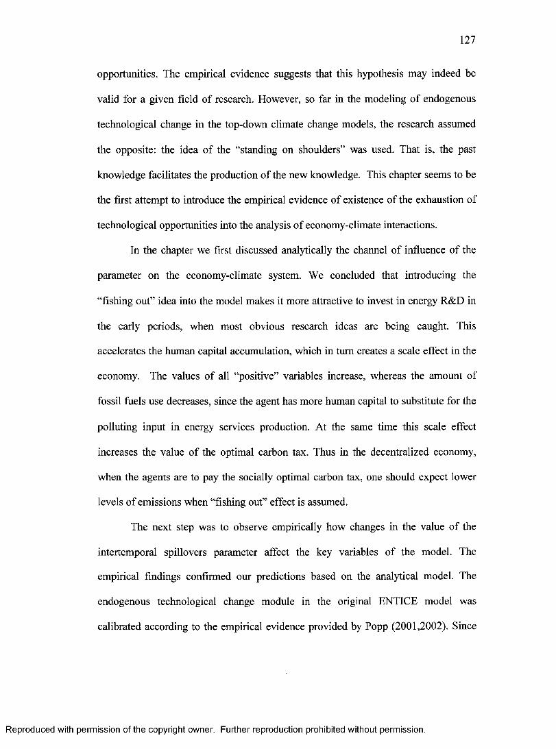
127

opportunities. The empirical evidence suggests that this hypothesis may indeed be

valid for a given field of research. However, so far in the modeling of endogenous

technological change in the top-down climate change models, the research assumed

the opposite: the idea of the “standing on shoulders” was used. That is, the past

knowledge facilitates the production of the new knowledge. This chapter seems to be

the first attempt to introduce the empirical evidence of existence of the exhaustion of

technological opportunities into the analysis of economy-climate interactions.

In the chapter we first discussed analytically the channel of influence of the

parameter on the economy-climate system. We concluded that introducing the

“fishing out” idea into the model makes it more attractive to invest in energy R&D in

the early periods, when most obvious research ideas are being caught. This

accelerates the human capital accumulation, which in turn creates a scale effect in the

economy. The values of all “positive” variables increase, whereas the amount of

fossil fuels use decreases, since the agent has more human capital to substitute for the

polluting input in energy services production. At the same time this scale effect

increases the value of the optimal carbon tax. Thus in the decentralized economy,

when the agents are to pay the socially optimal carbon tax, one should expect lower

levels of emissions when “fishing out” effect is assumed.

The next step was to observe empirically how changes in the value of the

intertemporal spillovers parameter affect the key variables of the model. The

empirical findings confirmed our predictions based on the analytical model. The

endogenous technological change module in the original ENTICE model was

calibrated according to the empirical evidence provided by Popp (2001,2002). Since


128

the calculation of the BAU scenario in the original ENTICE model by Popp (2004) is

based on the theoretically inconsistent approach, the whole model was re-calibrated

according to the empirical benchmarks for two scenarios: “fishing out” and “ standing

on shoulders”.

Our results indicate a higher deviation between BAU and optimal policy

emissions when “fishing out” hypothesis is assumed: for example, 20.3% deviation in

2185 versus 17.9% in “standing on shoulders” economy.

Our results also indicate that the welfare gain due to endogenous

technological change in the economy that is characterized by “fishing out” effect is

higher. In particular, our results indicate that introduction of endogenous

technological change in the “fishing out” economy increases the welfare by 11.5%.

At the same time, the “standing on shoulders” economy reaches 9.8% in the welfare

gain. This result is explained by higher cost savings due to lower fossil fuels use in

the “fishing out” economy. As pointed out above, the agent in the FISH economy has

more human capital to substitute for the polluting input. Thus we show that the

“fishing out” effect has a potential to increase the welfare gain due to endogenous

technological change.


129

References

Abdih Y. and Joutz F., 2005. Relating the Knowledge Production Function to Total Factor productivity: An Endogenous Growth Puzzle. International Monetary Fund, IMF Working Papers: 05/74.

Furman J., Porter M., Stem S.,2002. The Determinants of National Innovative Capacity. Research Policy 31,pp. 899-933.

Gerlagh R. and Lise W. (2005) Carbon Taxes: A Drop in the Ocean, or a Drop that Erodes the Stone? The effect of Carbon Taxes on Technological Change. Ecological Economics 54. pp.241- 260

Jones C.,1995. R&D Based Models of Economic Growth. Journal of Political Economy 103, pp. 739-784.

Jones C. and Williams J .,2000. Too Much of a Good Thing? The Economics of Investment in R&D. Journal of Economic Growth 5, pp.65-85.

Kortum, S., 1997. Research, Patenting, and Technological Change. Econometrica 65 (6 ), pp. 1389-1419.

Nordhaus W., 2002. Modeling Induced Innovation in Climate-Change Policy. Technological Change and the Environment, edited by Griibler A. et al. Resources for the Future, Washington, DC, pp. 182-209.

Popp D., 2001. The Effect of New Technology on Energy Consumption, Resource and Energy Economics 23, pp. 215-239.

Popp D., 2002. Induced Innovation and Energy Prices. American Economic Review 92, pp. 160-180.


Popp D.,2005. Lessons from patents: Using Patents to Measure Technological Change in Environmental Models. Ecological Economics 54, pp. 209- 226.Popp D., 2006. ENTICE-BR: The Effects of Backstop Technology R&D on Climate Policy M odels. Energy Econom ics, 28(2), pp. 188-222.

Porter M. and Stem S., 2000. Measuring the ‘Ideas’ Production Function: Evidence from International Patent Output. Working Paper No. 7891, National Bureau of Economic Research, Cambridge, MA.


130

Romer P., 1990. Endogenous Technological Change. Journal of Political Economy 98, pp. 71-102.

Romer D., 2001. Advanced Macroeconomics. Second Edition. McGraw-Hill Higher Education.

Segestrom P.,1998. Endogenous Growth without Scale Effects. American Economic Review 8 8 , pp. 1290-1310.


Chapter 5

Conclusion

This thesis attempted to address a number of issues in the economics of

climate change that have not been studied before. In particular, in the second chapter

of the thesis we suggested a new theoretically consistent method of modeling and

computation of the business-as-usual (no-policy) scenario in a single region model of

climate and economy. In the third chapter we examined the trade-off between

scarcity and pollution considerations within the context of climate change problem.

The focus of the fourth chapter was on the role of technological change for the

climate change policies.


science. One of the most important questions for the economy-climate models is how

the world will adapt to the greenhouse externality if no action is taken to reduce the

emissions. In order to answer this question, researchers compute the business-as-usual

(BAU) scenario. The second chapter of the thesis discussed a family of integrated

assessment models: the seminal DICE 1994 model by Nordhaus and its extensions. In

the chapter we pointed out that there are no external pollution costs in the framework

of the DICE 1994 due to the specific feature of the model: the whole world is

modeled as single region with a single decision maker. We demonstrated that in this

case the climate damages are fully internalized even under business-as-usual scenario.

Our goal was to develop the method of modeling the business-as-usual scenario,

building on the theoretical base for the DICE class models where the greenhouse

externality comes into play. We divided the world into a large number of identical

131


132

regions and assumed non-cooperative behaviour of the regions. By means of a simple

analytical model we showed the strong theoretical grounds of our approach. We

applied our method to a number of existing frameworks and demonstrated the

divergence from the previous estimates of baseline scenarios.

In DICE model and some of its variants the emissions of greenhouse gases are

modeled as the by-product of the output production. This assumption significantly

simplifies the structure of the model. However, an important feature of the problem is

ignored: the issue of resource (fossil fuels) scarcity is neglected in those models.

There are two polar opinions in the literature: the first is that the supply of fuels is

virtually unlimited and it is a matter of technological progress to maintain the era of

cheap fuels indefinitely. The second opinion argues that the world is about to run out

of conventional fuels, which means that the climate change policies should not get the

priority in the world’s agenda. However, the formal analysis of whether the

environmental considerations are prevailing over the issues of scarcity has not yet

been performed in the context of the global warming issue. The objective of the

chapter was to consider the trade-off between the scarcity rent and pollution cost in

context of climate change problem and to evaluate the trade-off quantitatively. We

were aiming to define and find the “true” ratio of scarcity rent and pollution cost in

the model that is characterized by perfect certainty, presence of the central planner

and the equitable treatment of all generations. We have performed the numerical

simulations that allowed us to provide the quantitative assessment of the trade-off.

Up until now the endogenous technological change was ignored in the top-

down climate-economy models. There are a few examples of recent works, which


133

have endogenous technological change module. The role of technological change for

the climate change policies has become the focus of the fourth chapter. The empirical

evidence suggests the existence of exhaustion of technological opportunities within a

particular field of research. However, so far in the top-down models researchers

assumed that the past energy-related knowledge facilitates the production of the new

knowledge. We aimed to compare the effects of these two hypothesises on the climate

change policy.


ESSAYS ON POLLUTION, SCARCITY AND ENDOGENOUS …

Documents

Transcript of ESSAYS ON POLLUTION, SCARCITY AND ENDOGENOUS …