Essays in Risk Management for Crude Oil Markets
154
Essays in Risk Management for Crude Oil Markets by Abdullah Al Mansour A thesis presented to the University of Waterloo in fulfillment of the thesis requirement for the degree of Doctor of Philosophy in Applied Economics Waterloo, Ontario, Canada, 2012 c Abdullah Al Mansour 2012
Transcript of Essays in Risk Management for Crude Oil Markets
Essays in Risk Management for
Crude Oil Markets
by
Abdullah Al Mansour
A thesis
presented to the University of Waterloo
in fulfillment of the
thesis requirement for the degree of
Doctor of Philosophy
in
Applied Economics
Waterloo, Ontario, Canada, 2012
c© Abdullah Al Mansour 2012

I hereby declare that I am the sole author of this thesis. This is a true copy of the thesis,
including any required final revisions, as accepted by my examiners.
I understand that my thesis may be made electronically available to the public.
ii

Abstract
This thesis consists of three essays on risk management in crude oil markets. In the first
essay, the valuation of an oil sands project is studied using real options approach. Oil sands
production consumes substantial amount of natural gas during extracting and upgrading.
Natural gas prices are known to be stochastic and highly volatile which introduces a risk
factor that needs to be taken into account. The essay studies the impact of this risk factor
on the value of an oil sands project and its optimal operation. The essay takes into account
the co-movement between crude oil and natural gas markets and, accordingly, proposes two
models: one incorporates a long-run link between the two markets while the other has no
such link. The valuation problem is solved using the Least Square Monte Carlo (LSMC)
method proposed by Longstaff and Schwartz (2001) for valuing American options. The
valuation results show that incorporating a long-run relationship between the two markets
is a very crucial decision in the value of the project and in its optimal operation. The essay
shows that ignoring this long-run relationship makes the optimal policy sensitive to the
dynamics of natural gas prices. On the other hand, incorporating this long-run relationship
makes the dynamics of natural gas price process have a very low impact on valuation and
the optimal operating policy.
In the second essay, the relationship between the slope of the futures term structure,
or the forward curve, and volatility in the crude oil market is investigated using a measure
of the slope based on principal component analysis (PCA). The essay begins by reviewing
the main theories of the relation between spot and futures prices and considering the
implication of each theory on the relation between the slope of the forward curve and
volatility. The diagonal VECH model of Bollerslev et al. (1988) was used to analyze the
relationship between of the forward curve slope and the variances of the spot and futures
prices and the covariance between them. The results show that there is a significant
iii
quadratic relationship and that exploiting this relation improves the hedging performance
using futures contracts.
The third essay attempts to model the spot price process of crude oil using the notion
of convenience yield in a regime switching framework. Unlike the existing studies, which
assume the convenience yield to have either a constant value or to have a stochastic behavior
with mean reversion to one equilibrium level, the model of this essay extends the Brennan
and Schwartz (1985) model to allows for regime switching in the convenience yield along
with the other parameters. In the essay, a closed form solution for the futures price is
derived. The parameters are estimated using an extension to the Kalman filter proposed
by Kim (1994). The regime switching one-factor model of this study does a reasonable
job and the transitional probabilities play an important role in shaping the futures term
structure implied by the model.
iv

Acknowledgments
I offer my sincere gratitude to my supervisors, Dr. Margaret Insley and Dr. Tony
Wirjanto, for their continuous support during my doctoral study. Without their time
and energy they offered me, this project would have been very hard to complete. Their
knowledge, experience, commitment, guidance and patience have contributed a big part
of this thesis. I am also indebted to the other committee members, Dr. Dinghai Xu, Dr.
Alain-Desire Nimubona and Dr. Kenneth Vetzal for their discussions and comments on
my thesis
Of course my deepest gratitude go to my father, Mohammad Almansour. I owe to my
father something I can neither express nor repay. Thank you my father for your everlasting
support and continuous encouragement. I also would like to thank my mother, Dolayyel
Almansour, for the unconditional love and constant prayers which were like the light I see
through. Her voice over the phone was a great source of motivation, especially when I hear
her say: see you soon Abdullah.
Foremost amongst the individuals to whom I am thankful is my wife, Dalal Alhammad.
I owe her a grate favor that I am sure I will be still owing throughout my life. Indeed, It
is a great blessing to work in such a project with such an accompany filled with inspiring
love, support, patience and since of humor. I keep asking the God that whatever comes
out of this success to be a source of blessing and happiness to you.
I would like to thank my lovely sisters, Eman, Huda, and Lateefa for there love, concern
and encouragement. Special thanks to Lateefa for taking care of my Mom. I am also
thankful to my father-, mother-in-low, Hmoud Alhammad and Lolwah Alsabt, for their
concern and honest prayers. Special thanks to my grandmother in-low, Umm Ali Alsabt,
for her endless and honest prayers.
v

Many thanks to all my friends at Waterloo who made my graduate study very special
and my stay in Canada feel like home. In particular, Dr. Ahmad Alojairi, Dr. Walid
Bahamdan and Dr. Abdullah Basiouni. It is not the coffee we were drinking together
almost every day that would keep me awake late at night, it is the honest friendship, the
critical thinking and the great experience we shared that would keep me awake in my life.
By the way, it’s my turn!
I would like to thank the department of Economics for providing the support and
facilities I have needed to produce and complete my thesis.
vi

Dedication
To my parents... See you soon.
To my wife... Here you go.
To my little twins... Here I am.
vii
Table of Contents
List of Figures ix
List of Tables x
1 Introductory Chapter 1
2 The Impact of Stochastic Extraction Cost on the Value of an Exhaustible
Resource: the Case of the Alberta Oil Sands 8
2.1 Introduction . . . . . . . . . . . . . . . . . . . . . . . . . . . . . . . . . . . 8
2.2 Oil Sands Background . . . . . . . . . . . . . . . . . . . . . . . . . . . . . 11
2.3 Co-movement of Crude Oil and Natural Gas Prices . . . . . . . . . . . . . 14
2.4 Modeling the Dynamics of Natural Gas and Crude Oil Prices . . . . . . . . 20
2.4.1 Seasonality . . . . . . . . . . . . . . . . . . . . . . . . . . . . . . . 24
2.4.2 Futures Pricing . . . . . . . . . . . . . . . . . . . . . . . . . . . . . 24
2.4.3 Estimation Procedure . . . . . . . . . . . . . . . . . . . . . . . . . 28
2.5 Oil Sands Valuation Model . . . . . . . . . . . . . . . . . . . . . . . . . . . 29
viii
2.6 Data Description for Estimation and Simulation . . . . . . . . . . . . . . . 32
2.7 Results . . . . . . . . . . . . . . . . . . . . . . . . . . . . . . . . . . . . . . 36
2.7.1 Estimation Results . . . . . . . . . . . . . . . . . . . . . . . . . . . 37
2.7.2 Valuation Results . . . . . . . . . . . . . . . . . . . . . . . . . . . . 41
2.8 Concluding Remarks . . . . . . . . . . . . . . . . . . . . . . . . . . . . . . 49
3 The Relationship Between Volatility and the Forward Curve in Crude
Oil Markets 51
3.1 Introduction . . . . . . . . . . . . . . . . . . . . . . . . . . . . . . . . . . . 51
3.2 Theoretical Background . . . . . . . . . . . . . . . . . . . . . . . . . . . . 54
3.3 PCA Slope Measure . . . . . . . . . . . . . . . . . . . . . . . . . . . . . . 61
3.4 Volatilities Model Specification . . . . . . . . . . . . . . . . . . . . . . . . 65
3.5 Data Description . . . . . . . . . . . . . . . . . . . . . . . . . . . . . . . . 67
3.6 Estimation Methodology . . . . . . . . . . . . . . . . . . . . . . . . . . . . 73
3.7 Estimation Results . . . . . . . . . . . . . . . . . . . . . . . . . . . . . . . 75
3.8 Application: Minimum Variance Hedge Ratio . . . . . . . . . . . . . . . . 79
3.9 Concluding Remarks . . . . . . . . . . . . . . . . . . . . . . . . . . . . . . 82
4 Contango and Backwardation in the Crude Oil Market: A Regime Switch-
ing Approach 84
4.1 Introduction . . . . . . . . . . . . . . . . . . . . . . . . . . . . . . . . . . . 84
4.2 Convenience Yield in Commodities Price Modeling . . . . . . . . . . . . . 87
ix

4.3 Regime Switching Model Specification . . . . . . . . . . . . . . . . . . . . 89
4.4 Futures Pricing . . . . . . . . . . . . . . . . . . . . . . . . . . . . . . . . . 95
4.5 Estimation Methodology . . . . . . . . . . . . . . . . . . . . . . . . . . . . 96
4.6 Data Description . . . . . . . . . . . . . . . . . . . . . . . . . . . . . . . . 101
4.7 Estimation Results . . . . . . . . . . . . . . . . . . . . . . . . . . . . . . . 104
4.7.1 Model Comparison . . . . . . . . . . . . . . . . . . . . . . . . . . . 111
4.7.2 The Impact of the Transitional Probabilities . . . . . . . . . . . . . 112
4.8 Concluding Remarks . . . . . . . . . . . . . . . . . . . . . . . . . . . . . . 117
5 Conclusion 119
Bibliography 123
APPENDICES 132
A Appendix to Chapter 4 133
A.1 The Definition of the Q Measure . . . . . . . . . . . . . . . . . . . . . . . 133
A.2 Xt in the Q Measure . . . . . . . . . . . . . . . . . . . . . . . . . . . . . . 134
A.3 Futures Price Formula Derivation . . . . . . . . . . . . . . . . . . . . . . . 135
A.4 Hamilton (1994) Filtration Procedure . . . . . . . . . . . . . . . . . . . . . 136
x
List of Figures
2.1 WTI Crude Oil and HH Natural Gas Prices . . . . . . . . . . . . . . . . . 14
2.2 Crude Oil and Natural Gas Correlation . . . . . . . . . . . . . . . . . . . . 16
2.3 Crude Oil and Natural Gas Correlation Term Structure . . . . . . . . . . . 20
2.4 Example of Natural Gas Forward Curve . . . . . . . . . . . . . . . . . . . 34
2.5 Implied Forward Curves . . . . . . . . . . . . . . . . . . . . . . . . . . . . 40
2.6 Oil Sand Project Value . . . . . . . . . . . . . . . . . . . . . . . . . . . . . 42
2.7 The Impact of N. Gas Long Term Component Volatility . . . . . . . . . . . 43
2.8 Project Value as a Function of N. Gas Long Term component . . . . . . . 45
2.9 Impact of N. Gas Process on the Switching Prices Under Model I : Backwar-
dation Case . . . . . . . . . . . . . . . . . . . . . . . . . . . . . . . . . . . 46
2.10 Impact of N. Gas Process on the Switching Prices Under Model II : Back-
wardation Case . . . . . . . . . . . . . . . . . . . . . . . . . . . . . . . . . 47
2.11 Impact of N. Gas Process on the Switching Prices Under Model I : Contango
Case . . . . . . . . . . . . . . . . . . . . . . . . . . . . . . . . . . . . . . . 48
2.12 Impact of N. Gas Process on the Switching Prices Under Model II : Contango
Case . . . . . . . . . . . . . . . . . . . . . . . . . . . . . . . . . . . . . . . 50
xi

3.1 WTI Crude Oil Forward Curve at Different Points in Time . . . . . . . . . 52
3.2 PCA Loadings of the Futures Price Returns . . . . . . . . . . . . . . . . . 63
3.3 Loadings of the 1st PC of the Centered Futures Prices . . . . . . . . . . . . 64
3.4 Time Series of the Relative Slope Factor It . . . . . . . . . . . . . . . . . . 65
3.5 Time Series of the Slope Factor, It, and the Actual Spot Returns Volatility,
σa . . . . . . . . . . . . . . . . . . . . . . . . . . . . . . . . . . . . . . . . 71
3.6 Scatter Plot of the Slope Factor, It, and the Actual Spot Returns Volatility,
σa . . . . . . . . . . . . . . . . . . . . . . . . . . . . . . . . . . . . . . . . 72
3.7 Time Series of The Hedging Portfolio Return . . . . . . . . . . . . . . . . . 82
4.1 The Implied Forward Curve of Gibson and Schwartz (1990) Model . . . . . 90
4.2 Crude Oil Price and Return Series . . . . . . . . . . . . . . . . . . . . . . . 102
4.3 The Implied Term Structure of Futures . . . . . . . . . . . . . . . . . . . 106
4.4 Observation Classification into Regimes . . . . . . . . . . . . . . . . . . . . 108
4.5 The Impact of the Market Price of Regime Switching Risk . . . . . . . . . 109
4.6 Model Performance Compared to Gibson and Schwartz (1990) Model . . . 113
4.7 Model Performance Compared to Gibson and Schwartz (1990) Model . . . 114
4.8 Model Performance Compared to Gibson and Schwartz (1990) Model . . . 115
4.9 The Impact of the Transitional Probabilities . . . . . . . . . . . . . . . . . 118
xii

List of Tables
2.1 Operation Cost in Oil Sands Production . . . . . . . . . . . . . . . . . . . 13
2.2 The Long-run Slope of Crude Oil and Natural Gas . . . . . . . . . . . . . 18
2.3 Johansen’s Maximum-Likelihood Tests of Co-Integration . . . . . . . . . . 19
2.4 Hypothetical Oil Sands Project Characteristics . . . . . . . . . . . . . . . . 36
2.5 Descriptive Statistics of Crude Oil and Natural Gas Log Returns . . . . . . 37
2.6 The Kalman Filter Quasi Maximum Likelihood Estimation . . . . . . . . . 38
2.7 Fitting Error of Model I and Model II . . . . . . . . . . . . . . . . . . . . 39
2.8 Oil Sands Project Value (Values in Millions) . . . . . . . . . . . . . . . . . 44
3.1 Theories on forward prices and their implications . . . . . . . . . . . . . . 62
3.2 Prediction Power of Different Slope Measures . . . . . . . . . . . . . . . . 69
3.3 Descriptive Statistics . . . . . . . . . . . . . . . . . . . . . . . . . . . . . . 70
3.4 Unit Root Test Results . . . . . . . . . . . . . . . . . . . . . . . . . . . . . 73
3.5 Johansen’s Maximum-Likelihood Tests of Co-Integration . . . . . . . . . . 74
3.6 Maximum Likelihood Estimation Results . . . . . . . . . . . . . . . . . . . 76
xiii
3.7 Wald’s Test Results . . . . . . . . . . . . . . . . . . . . . . . . . . . . . . . 78
3.8 Contribution of the Forward Curve Slope on the Second Moments . . . . . 79
3.9 Hedge Portfolio Performance . . . . . . . . . . . . . . . . . . . . . . . . . . 81
4.1 Descriptive Statistics . . . . . . . . . . . . . . . . . . . . . . . . . . . . . . 103
4.2 Kim Filter Estimation Results of the B&S-RS Model . . . . . . . . . . . . 105
4.3 Kalman Filter Estimation Results of the G&S Two-factor Model . . . . . . 111
xiv

Chapter 1
Introductory Chapter
Interest in energy-related investments and risk management has been growing in recent
years. Among the important energy commodities is crude oil, which is characterized by
highly uncertain and volatile prices. Crude oil is an important component of economic and
business activities in any economy. Thus, understanding its price movement is crucial for
successful economic and business decisions. Moreover, crude oil, and energy commodities
in general, have become one of the most active alternative assets1 during recent years.
Most energy products, such as crude oil and natural gas, have very liquid futures contracts
that are traded in exchanges. Moreover, several investment vehicles tied to their prices
are available in the market, ranging from small mutual funds and exchange-traded funds
(ETF), to large over-the-counter contracts (e.g SWAP contracts). In addition to finan-
cial investments, recent increases in energy prices have induced a large inflow of capital
into energy projects. For example, according to the Canadian Energy Research Institute
(CERI), the oil sands industry in Alberta attracted in excess of $18 billion of investment
1Alternative assets are alternative to the traditional investments such as publicly-traded stocks, bondsand mutual funds, see Anson (2002)
1
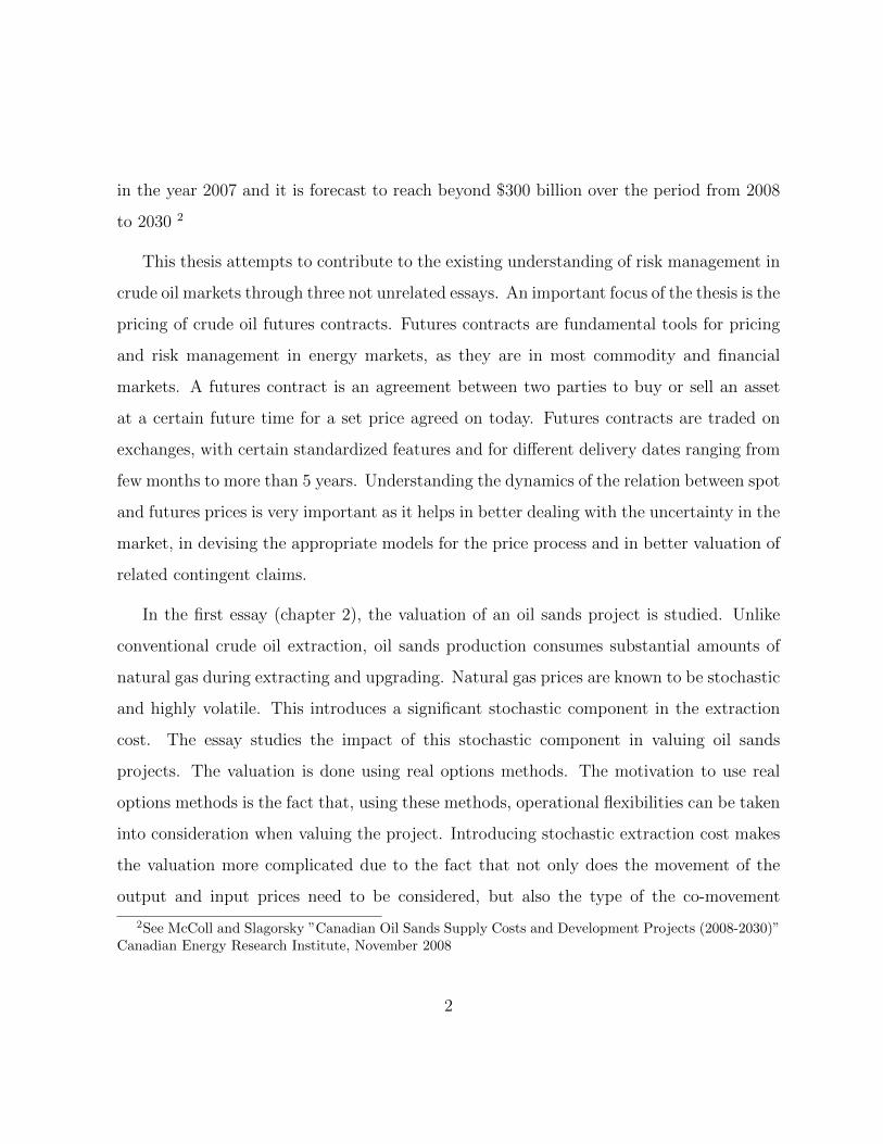
in the year 2007 and it is forecast to reach beyond $300 billion over the period from 2008
to 2030 2
This thesis attempts to contribute to the existing understanding of risk management in
crude oil markets through three not unrelated essays. An important focus of the thesis is the
pricing of crude oil futures contracts. Futures contracts are fundamental tools for pricing
and risk management in energy markets, as they are in most commodity and financial
markets. A futures contract is an agreement between two parties to buy or sell an asset
at a certain future time for a set price agreed on today. Futures contracts are traded on
exchanges, with certain standardized features and for different delivery dates ranging from
few months to more than 5 years. Understanding the dynamics of the relation between spot
and futures prices is very important as it helps in better dealing with the uncertainty in the
market, in devising the appropriate models for the price process and in better valuation of
related contingent claims.
In the first essay (chapter 2), the valuation of an oil sands project is studied. Unlike
conventional crude oil extraction, oil sands production consumes substantial amounts of
natural gas during extracting and upgrading. Natural gas prices are known to be stochastic
and highly volatile. This introduces a significant stochastic component in the extraction
cost. The essay studies the impact of this stochastic component in valuing oil sands
projects. The valuation is done using real options methods. The motivation to use real
options methods is the fact that, using these methods, operational flexibilities can be taken
into consideration when valuing the project. Introducing stochastic extraction cost makes
the valuation more complicated due to the fact that not only does the movement of the
output and input prices need to be considered, but also the type of the co-movement
2See McColl and Slagorsky ”Canadian Oil Sands Supply Costs and Development Projects (2008-2030)”Canadian Energy Research Institute, November 2008
2

of the two prices must be taken into account. Given this fact, the essay begins with
an investigation of the empirical literature about the nature of the co-movement between
crude oil and natural gas prices. In particular, I consider whether there is a long-term effect
that results from an economic relationship between crude oil and natural gas or whether
the co-movement arises only from a short-term effect associated with the correlation of
the energy prices. For the valuation section of this essay, the stochastic dynamics of the
oil and gas prices are modeled using the two-factor model of Schwartz and Smith (2000)
in a multi-commodity framework. In general, two-factor models have proved to capture
the historical dynamics and the term structure of commodities futures fairly well. More
importantly, the Schwartz and Smith (2000) framework allows us to distinguish between
the long- the short-run movements of the commodity prices and thus enables us to model
the long- and the short-run co-movements in the two markets in an explicit way. The
valuation problem is solved by the Least Square Monte Carlo (LSMC) method proposed
by Longstaff and Schwartz (2001) for valuing American options. The LSMC proved to be
an efficient tool for valuing high order problems, where the number of stochastic factors
are large as it is the case in this essay where there are four factors: two for crude oil prices
and two for natural gas prices.
In the second essay (chapter 3), the relationship between the slope of the futures term
structure and volatility in the crude oil market is investigated. The futures term structure,
or simply the forward curve3, is a plot of the futures prices against their corresponding
maturities at a specific point in time. Generally, the forward curve can take many shapes.
However, there are two main shapes that market participants usually pay attention to:
a positive slope forward curve which is known as contango and a negative slope forward
curve which is known as backwardation. Many studies have documented the significance
3 Both terms, the futures term structure and the forward curve will be used interchangeably.
3
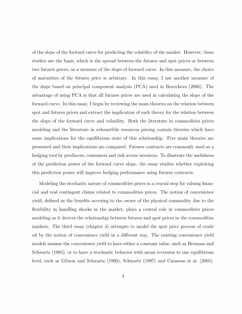
of the slope of the forward curve for predicting the volatility of the market. However, these
studies use the basis, which is the spread between the futures and spot prices or between
two futures prices, as a measure of the slope of forward curve. In this measure, the choice
of maturities of the futures price is arbitrary. In this essay, I use another measure of
the slope based on principal component analysis (PCA) used in Borovkova (2006). The
advantage of using PCA is that all futures prices are used in calculating the slope of the
forward curve. In this essay, I begin by reviewing the main theories on the relation between
spot and futures prices and extract the implication of each theory for the relation between
the slope of the forward curve and volatility. Both the literature in commodities prices
modeling and the literature in exhaustible resources pricing contain theories which have
some implications for the equilibrium state of this relationship. Five main theories are
presented and their implications are compared. Futures contracts are commonly used as a
hedging tool by producers, consumers and risk averse investors. To illustrate the usefulness
of the prediction power of the forward curve slope, the essay studies whether exploiting
this prediction power will improve hedging performance using futures contracts.
Modeling the stochastic nature of commodities prices is a crucial step for valuing finan-
cial and real contingent claims related to commodities prices. The notion of convenience
yield, defined as the benefits accruing to the owner of the physical commodity due to the
flexibility in handling shocks in the market, plays a central role in commodities prices
modeling as it derives the relationship between futures and spot prices in the commodities
markets. The third essay (chapter 4) attempts to model the spot price process of crude
oil by the notion of convenience yield in a different way. The existing convenience yield
models assume the convenience yield to have either a constant value, such as Brennan and
Schwartz (1985), or to have a stochastic behavior with mean reversion to one equilibrium
level, such as Gibson and Schwartz (1990), Schwartz (1997) and Casassus et al. (2005).
4
The model of this essay extends the Brennan and Schwartz (1985) model to allows for
regime switching in the convenience yield. The motivations behind this choice of modeling
are the following. Theoretically, the convenience yield is seen as a function of the level of
the commodity inventory in the economy which is in turn a function of the supply and
demand conditions. Moreover, macroeconomic conditions which run through different cy-
cles of booms and busts are likely to have impacts on the commodities markets especially
for crucial commodities such as crude oil. Given that, it is unlikely that there is only one
equilibrium state the commodity market should revert to. From the empirical side, esti-
mating the Gibson and Schwartz (1990) model using crude oil futures in different periods
of time produces very different values of the equilibrium level of convenience yield.
The regime switching approach to modeling provides a natural way to relax this re-
strictive assumption about the level of the convenience yield. Regime-switching models are
time-series models in which parameters are allowed to take on different values in each of
some fixed number of regimes or states. A stochastic process assumed to have generated
the regime shifts is included as part of the model, which allows for model-based forecasts
that incorporate the possibility of future regime shifts. The primary use of these models
in econometrics has been to describe changes in the dynamic behavior of macroeconomic
and financial time series (Hamilton (1994) and Dai et al. (2007)).
The model of this essay is different from those of Chen and Forsyth (2010) and Chen
(2010) who take regime switching approach to model energy prices in three main ways.
First, the regime switching model proposed in their studies is based on the one-factor
model applied in Schwartz (1997) where the commodity price reverts to different levels
with different volatilities. In this essay, the convenience yield switches to different levels
with different volatilities. Second, unlike their studies, the model of this essay allows for
pricing the risk of switching between the regimes. Third, they calibrate the parameters
5
of the model by solving the partial deferential equation (PDE) characterizing the futures
price numerically and calibrate the solution to the observed futures prices using least
square methods. The model of this essay is estimated using an extension to the Kalman
filter procedure proposed by Kim (1994). The choice of the Kalman filter procedure for
estimating the model is motivated by the Monte Carlo study of Duffee and Stanton (2004)
in estimating the term structure of interest rates where Kalman filtering procedure is found
to be a tractable and reasonably accurate estimation technique. To judge the performance
of the model of this study, it is compared with Gibson and Schwartz (1990) two- factor
model.
Overall, the dissertation contributes to our understanding about risk management in
crude oil markets in a number of ways.
• The thesis contributes to the literature about the co-movement of crude oil and
natural gas prices by investigating the type of the co-movement using the futures
prices of the two markets and proposing a way of modeling the two types of the
co-movement that can be easily estimated by the term structure of futures prices in
the two markets.
• The thesis contributes to the literature of real options valuation of exhaustible re-
sources by studying the value of an oil sands project. In particular, the thesis studies
how a stochastic extraction cost can affect the value of an exhaustible resource.
• It also contributes to the understanding of the relation between volatility and the
slope of the forward curve in two ways: by extracting the implications of various
theoretical work on this relation; and by analyzing the relation empirically using a
more appropriate measure of the forward curve slope extracted by PCA.
6
• The thesis also contributes to the literature about commodity prices modeling by
proposing a regime switching model that is more appropriate for convenience yield
modeling especially for long-run valuation purposes. Moreover, the thesis shows how
a closed form solution for the futures price formula can be obtained.
The main results of the dissertation are as follows:
• The analysis of the first essay shows that higher natural gas price volatility reduces
the value of the project. It also shows that not only the dynamics of oil and natural
gas prices are important, but also the nature of the co-movement of the two prices
is an important factor to take into consideration in valuation and optimal operation.
While the economic links between the two markets, i.e. being substitutes as sources
of energy, suggests the existence of a long-run relationship between the two prices,
the empirical evidence is weak especially if one incorporates the recent divergence
in the two price series. The valuation results show that incorporating a long-run
relationship between the two markets is a very crucial decision in valuing the project
and in its optimal operation. It is shown that ignoring this long-run relationship
makes the optimal policy more sensitive to the dynamics of natural gas prices.
• In the second essay, it is found that the forward curve slope has no significant linear
impact on the variances of the futures and spot prices and the covariance between
them. However, the slope of the forward curve does have a significant quadratic
impact not only on the variance of spot and futures price returns as Carlson et al.
(2007) and Kogan et al. (2009) found, but also in the covariance between the two
prices. Moreover, it is shown that incorporating the slope of the forward curve
quadratically produces a significant improvement in the hedging performance using
futures contracts.
7
• Compared to the performance of the Gibson and Schwartz (1990) two-factor model,
the regime switching one-factor model of the third essay does a reasonable job. In
particular, the model outperforms the Gibson and Schwartz (1990) model for fitting
the prices of far maturities contracts. Moreover, the transitional probabilities have
been found to play an important role in producing various shapes of the futures term
structure that are commonly seen in the market.
8
Chapter 2
The Impact of Stochastic Extraction
Cost on the Value of an Exhaustible
Resource: the Case of the Alberta
Oil Sands
2.1 Introduction
Traditionally, valuing a natural resource project, or any project in general, is based on
the simple net present value method. Using this method, expected future cash flows from
operating a project are discounted to the current time using a constant risk adjusted
discount rate and added up to give the value of the project. This procedure has been
criticized for ignoring possible flexibilities in starting or operating the project. Examples
of such ignored flexibilities are: the flexibility in starting the investment (option to delay)
9

and the flexibility to switch between different mode of operations (option to switch). In
addition, the use of a constant risk adjusted discount rate is known to be inappropriate
for valuing projects 1.
On the other hand, in the real options valuation approach, managerial flexibilities are
taken into consideration when valuing a project. In general, the real options approach is
based on the analogy between financial options and investment projects, and thus it uses
the valuation tools developed for financial options. For more details on this method and
its features, see Dixit and Pindyck (1994) and Schwartz and Trigeorgis (2004).
In their seminal paper, Brennan and Schwartz (1985) set the ground for using contingent
claims analysis for valuing an exhaustible natural resources when the decision-maker has
flexibility to choose from multiple modes of operation. The uncertainty in their model has
only one source, the output price. They assumed fixed extraction cost and that the price
follows Geometric Brownian Motion (GBM)2.
Many papers account for more realistic assumptions about the sources of the uncertainty
faced by an exhaustible resource. Cortazar et al. (2008) and Tsekrekos et al. (2010) ex-
tended Brennan and Schwartz (1985) valuation problem under different output price model
dynamics. Cortazar et al. (2001) studied the valuation of natural resource exploration in-
vestments when there is joint price and geological-technical uncertainty. Armstrong et al.
(2004) accounts for the uncertainty in the reserve.
However, one aspect that seems to be ignored in this literature, valuing exhaustible
1 For valuating a copper mine using the real options approach, Brennan and Schwartz (1985) showedthat the risk of the mine is function of the spot price of copper which is stochastic. Thus, the instantaneousrate of return required by investors should be stochastic, showing the inappropriateness of assuming aconstant discount rate in the present value analysis.
2Brownian motion is a continuous-time stochastic process that has independent increments of normaldistribution with mean of zero and variance of the time difference, i.e. if z(t) is a Brownian motion thendz(t) ∼ N(0, dt). For more details see Klebaner (2005)
10
resources using contingent clams analysis, is the possibility that production cost or part
of it, along with other state variables, is stochastic and volatile as well. An exception is
Slade (2001) who used yearly panel data about 21 copper mines in Canada from the 1980
to 1993 period and found that average costs, which include the costs of mining, milling,
smelting, refining, shipping, and marketing, to be highly variable. Using these data, Slade
(2001) then applied the real options theory to Canadian mining investments and studied
the impact of copper price, average cost and resource reserve uncertainties under different
assumptions about the stationarity of the stochastic processes.
The lack of studies that account for stochastic cost is possibly because of the difficulty
of obtaining enough data on cost variables as is the case in Slade (2001). This makes
the variability in cost hard to appreciate. A perfect example where the uncertainty of
extraction cost appears to be salient is the oil sands industry. The oil sands industry
consumes substantial amounts of natural gas during production and upgrading activities.
According to the Canadian Energy Research Institute (CERI), natural gas, its price being
highly volatile, contributes more than 25 percent of the total per barrel supply cost3. "In
2007, the oil sands industry accounted for approximately 1.0 billion cubic feet per day
(bcf/d) of natural gas demand, slightly more than 40 percent of Alberta total natural gas
demand of 2.7 bcf/d"4.
Two features characterize the source of uncertainty about extraction cost in the oil sands
industry. First, data about natural gas prices is readily available on a daily basis. Second,
crude oil and natural gas markets are linked together and thus, for better valuation and risk
management decisions, modeling the nature of their co-movement should be considered.
3The supply cost is the constant dollar price needed to recover all capital expenditures, operating costs,royalties, taxes, and earn a specified return on investment
4see McColl and Slagorsky, ”Canadian Oil Sands Supply Costs and Development Projects (2008-2030)”Canadian Energy Research Institute, 2008
11
Accordingly, this chapter examines the nature of the co-movement of crude oil and natural
gas markets and then studies the impact of the stochastic extraction cost on the valuation
of an oil sands project. In particular, two extensions of the Schwartz and Smith (2000)
model to specify the stochastic dynamics of the two prices are suggested and the Brennan
and Schwartz (1985) valuation problem is solved.
As shown in Brennan and Schwartz (1985), an analytical solution to such a problem
is unavailable, so they solve the problem using a finite difference numerical methods. Re-
cent developments in valuing American options using simulation based methods enable
researchers to explore more realistic extensions to the Brennan and Schwartz (1985) model
that proved to be impractical to solve using the prevailing numerical methods such as finite
difference or lattice methods. The Least Square Monte Carlo (LSMC) method developed
by Longstaff and Schwartz (2001) has proved to be an efficient tool for valuing complex
real options problems. Gamba (2003) provides a comprehensive overview on how LSMC
could be used to value various types of real options. Accordingly, LSMC is used for the
purpose of this chapter. Cortazar et al. (2008) and Tsekrekos et al. (2010) also used this
method for solving real options valuation problems.
This chapter is organized as follows: section 2.2 gives a background on the oil sands
industry. Section 2.3 reviews the empirical literature on the co-movement of natural gas
and crude oil markets with some recent results. Sections 2.4 and 2.5 specify the modeling
procedures of the state variables and the oil sands project to be used in estimation and
simulation. Data description and results are given in sections 2.6 and 2.7 respectively. The
last section is for concluding remarks.
12
2.2 Oil Sands Background
The oil sands are unevenly spread over 140,000 km2 (54,000 square miles) in Northern
Alberta, Canada. The area contains an estimated 1.7 trillion barrels (initial volume-in-
place) of an extremely heavy crude oil referred to as bitumen5. This reserve is believed to
be a valuable energy source given its size, the current and expected high prices of crude oil
and the state of the global supply and demand of the oil market. According to Canadian
Association of Petroleum Producers (CAPP), capital expenditure in oil sands projects has
risen from $4.2 billion in 2000 to $11.2 billion in 2009. 6
Approximately 20 percent of of Alberta’s oil sands can be found close enough under the
surface (generally less than 75 meters) to permit mining production. On the other hand,
around 80 percent of this reserve is found too deep below the surface for feasible mining
operations. Bitumen in such deep deposits (typically 400 meters below the surface) needs
to be recovered from the in situ (Latin: in place) position, similar to conventional oil, but
by using a variety of special production techniques.
In in situ extraction techniques, a high temperature steam is injected inside the bitumen
deposit through horizontal or vertical wells to reduce its viscosity and make it easier to be
pumped up to the surface. The steam generators used within the process use natural gas
as a fuel source. According to CERI, a rule-of-thumb commonly used in the industry is
that 1 Mcf (thousand cubic feet) of natural gas is required to produce a barrel of bitumen.
It is estimated that natural gas usage amounts to about 45 percent of total per-barrel
operating cost. Table 2.1 shows the per-barrel of bitumen operating cost for a typical in
5Crude bitumen, or bitumen, is a term that reflects the heavy and highly viscous oil in the oil sandsareas. The term ”oil sands” includes the crude bitumen, minerals, and rocks that are found together withthe bitumen (www.ERCB.com)
6 See 2011 Statistical Handbook in (http://www.capp.ca).
13

Table 2.1. Operation Cost for Bitumen In situ Production (Canadian Dollars)
Operating Cost (Excluding Energy)
Fixed Operation Cost $ 47.6 Million per yearVariable Operating Cost $ 6.6 per barrel
Natural Gas Cost $ 7.5 per barrel
Total (for capacity of 30,000 barrel per day) $ 18 per barrelTotal (WTI equivalent) $ 35 per barrel
Source: Canadian Energy Research Institute (CERI), 2008
situ project.
A typical in situ oil sands plant consists of multiple well pads containing a group of wells
where bitumen is extracted and a central processing facility (CPF) where the extracted
bitumen is processed to meet certain specifications. Steam from the CPF is transported
by pipelines to the well pads and distributed to the various wells. Produced water and
bitumen from the wells are then taken back for processing in the CPF. The majority of the
bitumen is upgraded to produce synthetic crude oil (SCO). Given this heavy dependency
on natural gas in bitumen production, uncertainty in natural gas prices is an important
risk factor that needs to be accounted for. Natural gas prices are characterized by high
volatility and high correlation with other energy prices especially with the oil prices (see
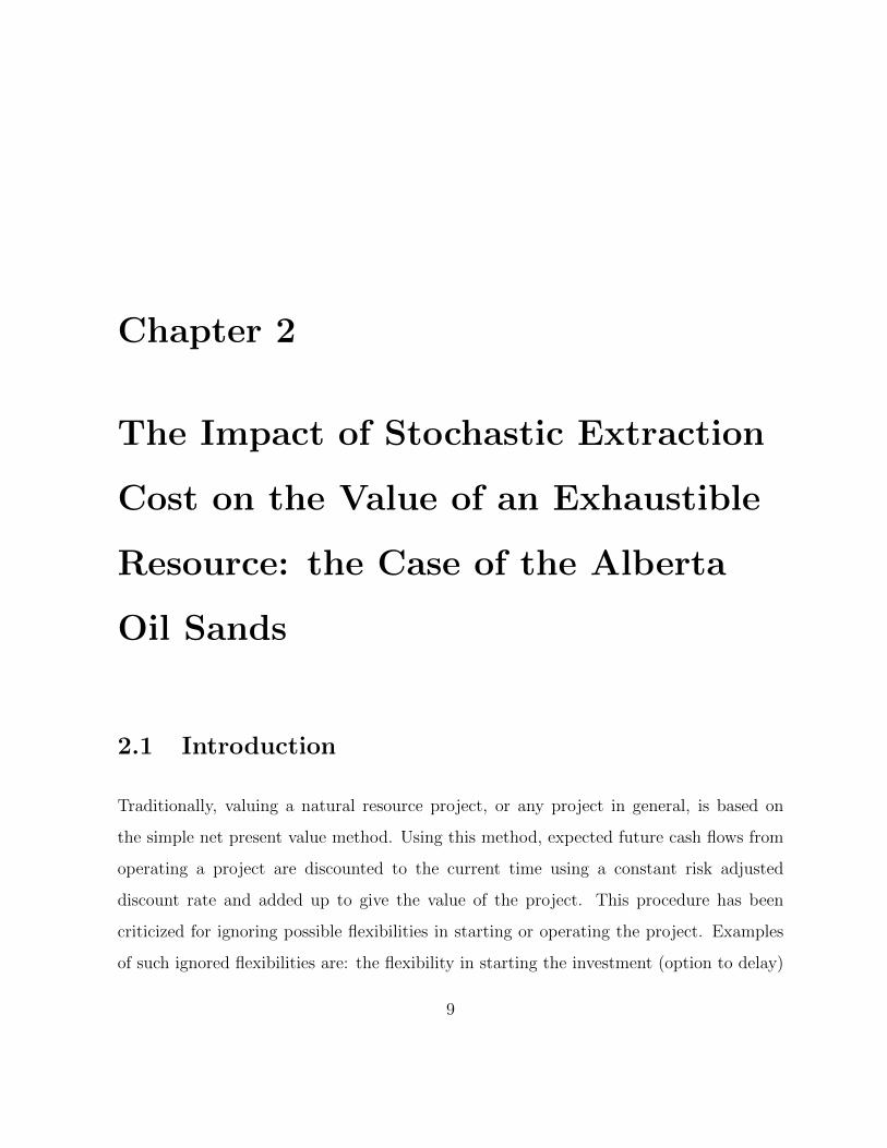
Pindyck (2004), Geman (2005) and Brown and Yucel (2007)). Figure 2.1 shows the price
of natural gas at Henry Hub, a major trading point located in the south of the US on
the Gulf of Mexico, along with the price of WTI crude oil from 1997 until 2010. A casual
inspection of the graph indicates that the price of natural gas tends to move with the price
of oil, but not always. The next section studies this co-movement in detail.
In this chapter, I study the impact of this risk factor on the value and the optimal
14

operation of an oil sands project. While the application is for oil sands industry, the
analysis and insights are applicable to a variety of large natural resource projects that
requires a significant amount of a volatile input with a volatile price.
2.3 Co-movement of Crude Oil and Natural Gas Prices
In general, there are two sources of co-movement among commodities as explained in
Casassus et al. (2010). The first one is a short-term effect associated with the correlation
of commodity prices while the second source arises from a long-term effect that results
from an economic relationship such as a production relationship where one commodity
is produced from another one and substitution relationship where two commodities are
substitutes in consumption. Figure 2.1 shows the time series of the price of crude oil
and natural gas. It appears from the graph that the two commodity prices tend to move
together. The correlation coefficient is 0.26 between their (log) differences and 0.75 between
their levels.
Villar and Joutz (2006) identify several economic factors that link natural gas and crude
oil prices, from both supply and demand sides. One of the main links is the competition
between natural gas and petroleum products which occurs principally in the industrial and
electric generation sectors. Industry and electric power generators switch back and forth
between natural gas and residual fuel oil, using whichever energy source is least expensive.
Some empirical studies confirm this fact, finding a long-run relationship between the
two commodity price series. Villar and Joutz (2006) studied the co-movement of the two
prices over the period from 1989 through 2005 and found oil and natural gas prices to be co-
integrated with a trend. Brown and Yucel (2007) examined the relationship between weekly
prices over the period from January 7, 1994 through July 14, 2006. Their analysis revealed
15
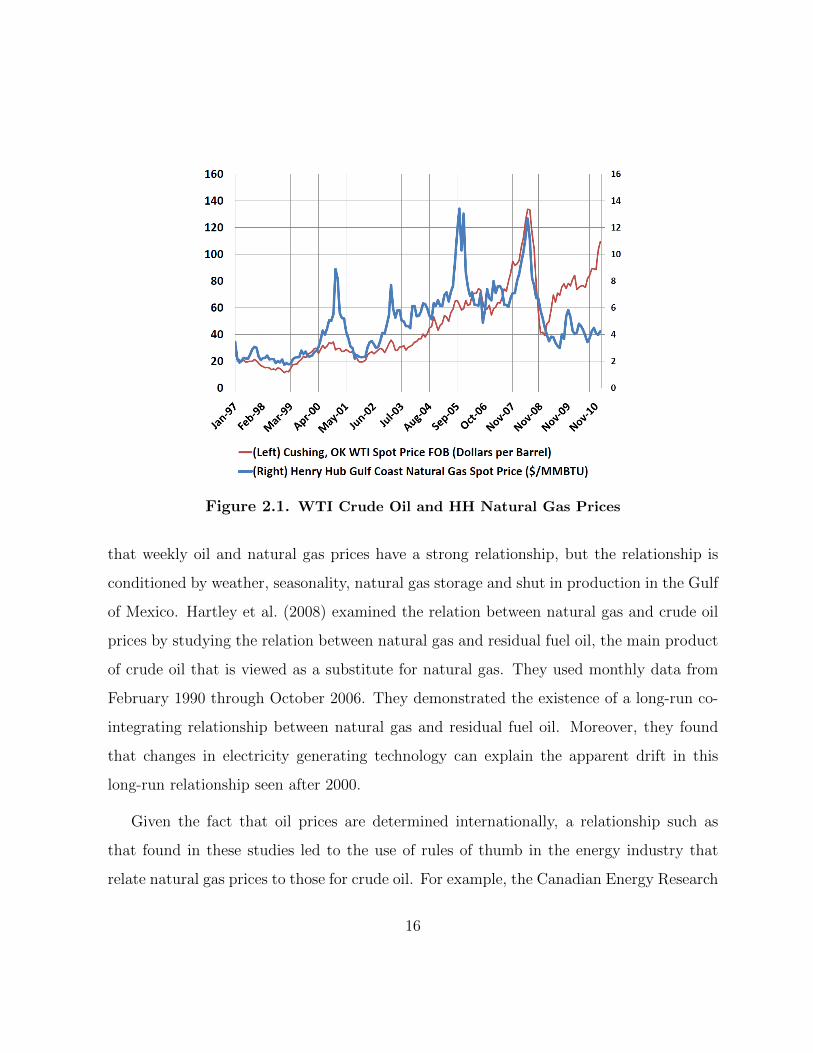
Figure 2.1. WTI Crude Oil and HH Natural Gas Prices
that weekly oil and natural gas prices have a strong relationship, but the relationship is
conditioned by weather, seasonality, natural gas storage and shut in production in the Gulf
of Mexico. Hartley et al. (2008) examined the relation between natural gas and crude oil
prices by studying the relation between natural gas and residual fuel oil, the main product
of crude oil that is viewed as a substitute for natural gas. They used monthly data from
February 1990 through October 2006. They demonstrated the existence of a long-run co-
integrating relationship between natural gas and residual fuel oil. Moreover, they found
that changes in electricity generating technology can explain the apparent drift in this
long-run relationship seen after 2000.
Given the fact that oil prices are determined internationally, a relationship such as
that found in these studies led to the use of rules of thumb in the energy industry that
relate natural gas prices to those for crude oil. For example, the Canadian Energy Research
16

Institute (CERI) in its 2009 report about Canadian oil sands supply costs and development
projects7 assumed that there is a 10:1 ratio between the price of oil in $/barrel and the
price of natural gas in mm Btu8. Other rule of thumbs have also been used as shown in
Brown and Yucel (2007).
However, other empirical studies find a weak or no long-run relationship between the
two prices. Serletis and Rangel-Ruiz (2004) explored the strength of shared trends and
shared cycles between natural gas and crude oil markets. Using daily data from January
1991 to April 2001, their results show that there has been a decoupling of the prices
of these two sources of energy and they explained that this was a result of oil and gas
deregulation. Bachmeier and Griffin (2006) found that the degree of the co-integration
between the two prices was very weak during the period from 1990 to 2004. Mohammadi
(2009) analyzed annual and monthly data of the period from 1970 to 2007 and found a
lack of co-integration relationship in the annual data and a weak one in the monthly data.
Moreover, he examined the possibility of co-integration with asymmetric adjustments using
threshold autoregressive (TAR) models. The results again fail to reject the null hypothesis
of no co-integration.
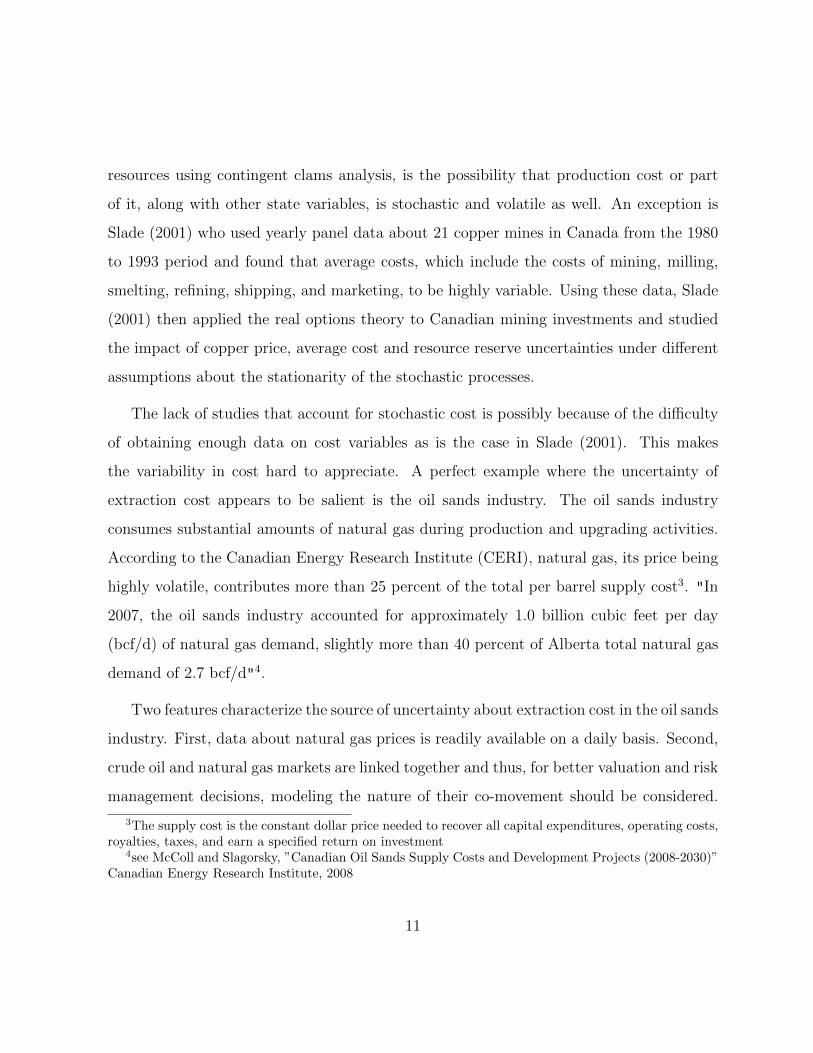
Figure 2.2 shows the correlation coefficient between the daily returns of the two com-
modity prices in each month. It is clear from the graph that the correlation between the
two price movements has gone through up and down cycles. In the late 90’s, the corre-
lation was relatively low, around 0.1. From 2003 to 2008, one can identify a cycle of a
high co-movement, the correlation coefficient was around 0.4 on average. This cycle has
7See McColl, Mei, Millington and Slagorsky ”Canadian Oil Sands Supply Costs and DevelopmentProjects (2009-2043)” Canadian Energy Research Institute, November 2009
8 mm Btu stands for 10,000 million British thermal units. Natural gas can also be measured ingigajoule(GJ) and thousand cubic feet (Mcf). NYMEX Henry Hub natural gas prices are quoted in mmBtu. The relation between these three measures are: 1 mm BTU = 1.027 Mcf =1.05 GJs
17
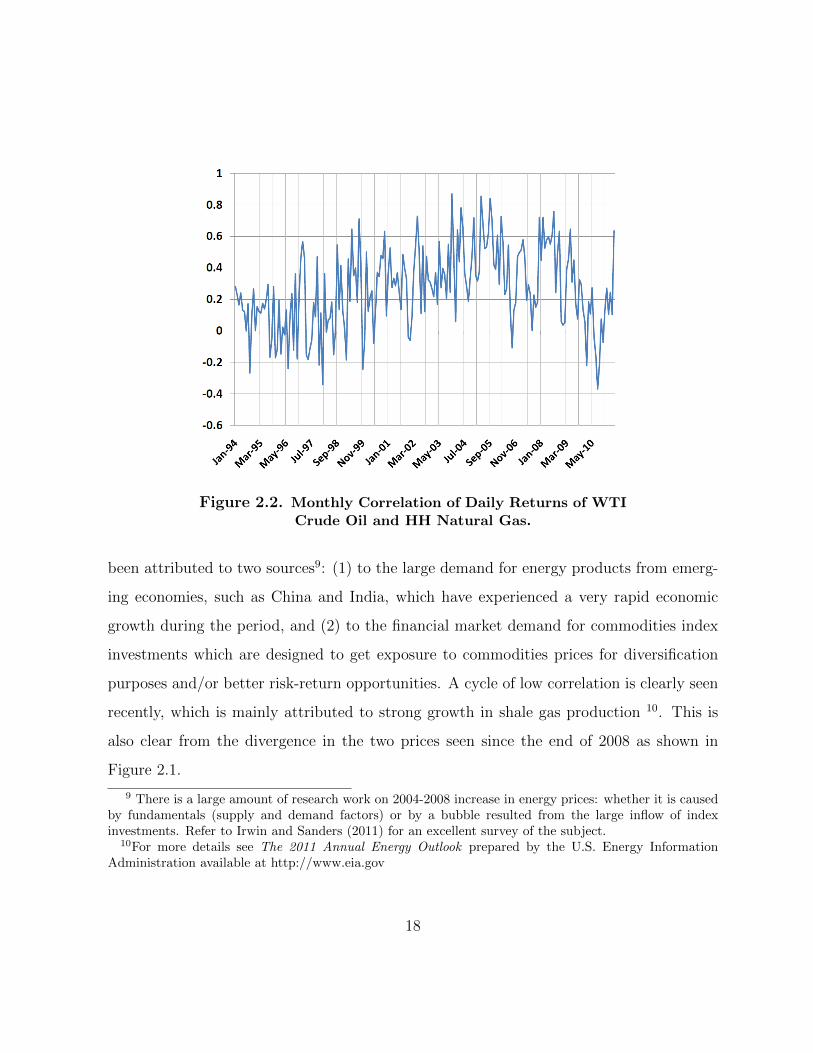
Figure 2.2. Monthly Correlation of Daily Returns of WTICrude Oil and HH Natural Gas.
been attributed to two sources9: (1) to the large demand for energy products from emerg-
ing economies, such as China and India, which have experienced a very rapid economic
growth during the period, and (2) to the financial market demand for commodities index
investments which are designed to get exposure to commodities prices for diversification
purposes and/or better risk-return opportunities. A cycle of low correlation is clearly seen
recently, which is mainly attributed to strong growth in shale gas production 10. This is
also clear from the divergence in the two prices seen since the end of 2008 as shown in
Figure 2.1.
9 There is a large amount of research work on 2004-2008 increase in energy prices: whether it is causedby fundamentals (supply and demand factors) or by a bubble resulted from the large inflow of indexinvestments. Refer to Irwin and Sanders (2011) for an excellent survey of the subject.
10For more details see The 2011 Annual Energy Outlook prepared by the U.S. Energy InformationAdministration available at http://www.eia.gov
18
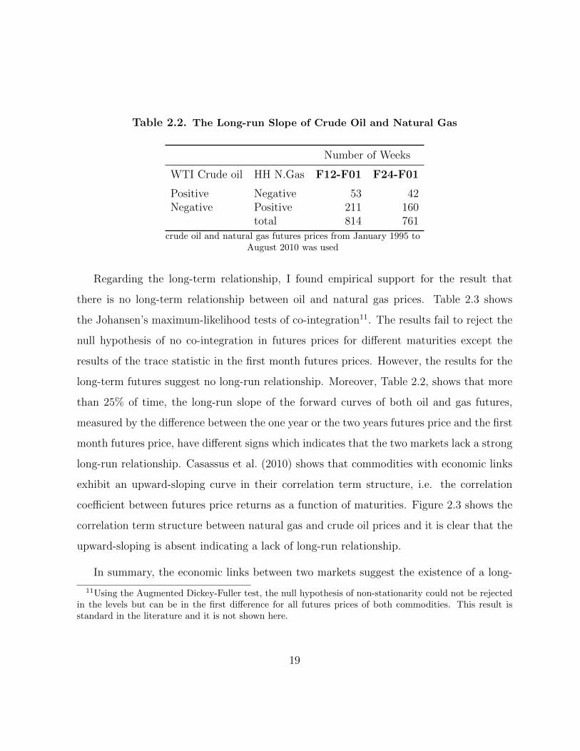
Table 2.2. The Long-run Slope of Crude Oil and Natural Gas
Number of Weeks
WTI Crude oil HH N.Gas F12-F01 F24-F01
Positive Negative 53 42Negative Positive 211 160
total 814 761
crude oil and natural gas futures prices from January 1995 toAugust 2010 was used
Regarding the long-term relationship, I found empirical support for the result that
there is no long-term relationship between oil and natural gas prices. Table 2.3 shows
the Johansen’s maximum-likelihood tests of co-integration11. The results fail to reject the
null hypothesis of no co-integration in futures prices for different maturities except the
results of the trace statistic in the first month futures prices. However, the results for the
long-term futures suggest no long-run relationship. Moreover, Table 2.2, shows that more
than 25% of time, the long-run slope of the forward curves of both oil and gas futures,
measured by the difference between the one year or the two years futures price and the first
month futures price, have different signs which indicates that the two markets lack a strong
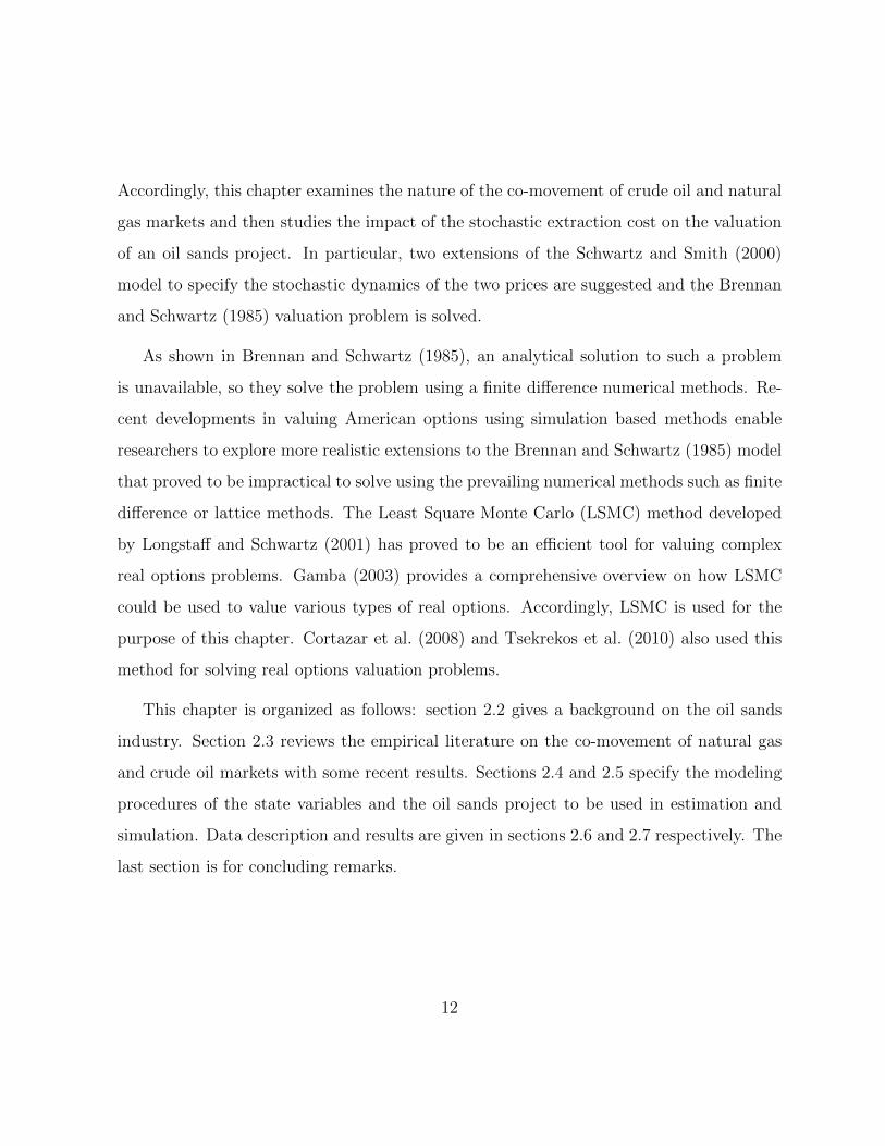
long-run relationship. Casassus et al. (2010) shows that commodities with economic links
exhibit an upward-sloping curve in their correlation term structure, i.e. the correlation
coefficient between futures price returns as a function of maturities. Figure 2.3 shows the
correlation term structure between natural gas and crude oil prices and it is clear that the
upward-sloping is absent indicating a lack of long-run relationship.
In summary, the economic links between two markets suggest the existence of a long-
11Using the Augmented Dickey-Fuller test, the null hypothesis of non-stationarity could not be rejectedin the levels but can be in the first difference for all futures prices of both commodities. This result isstandard in the literature and it is not shown here.
19
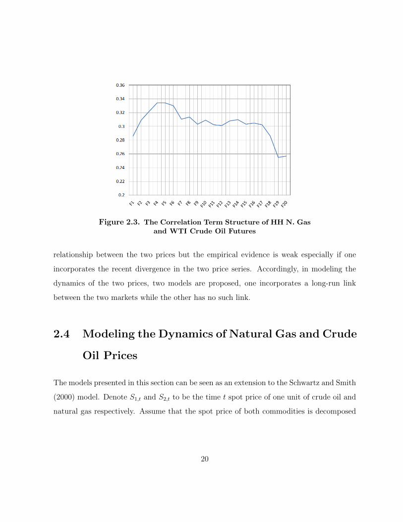
Figure 2.3. The Correlation Term Structure of HH N. Gasand WTI Crude Oil Futures
relationship between the two prices but the empirical evidence is weak especially if one
incorporates the recent divergence in the two price series. Accordingly, in modeling the
dynamics of the two prices, two models are proposed, one incorporates a long-run link
between the two markets while the other has no such link.
2.4 Modeling the Dynamics of Natural Gas and Crude
Oil Prices
The models presented in this section can be seen as an extension to the Schwartz and Smith
(2000) model. Denote S1,t and S2,t to be the time t spot price of one unit of crude oil and
natural gas respectively. Assume that the spot price of both commodities is decomposed
20
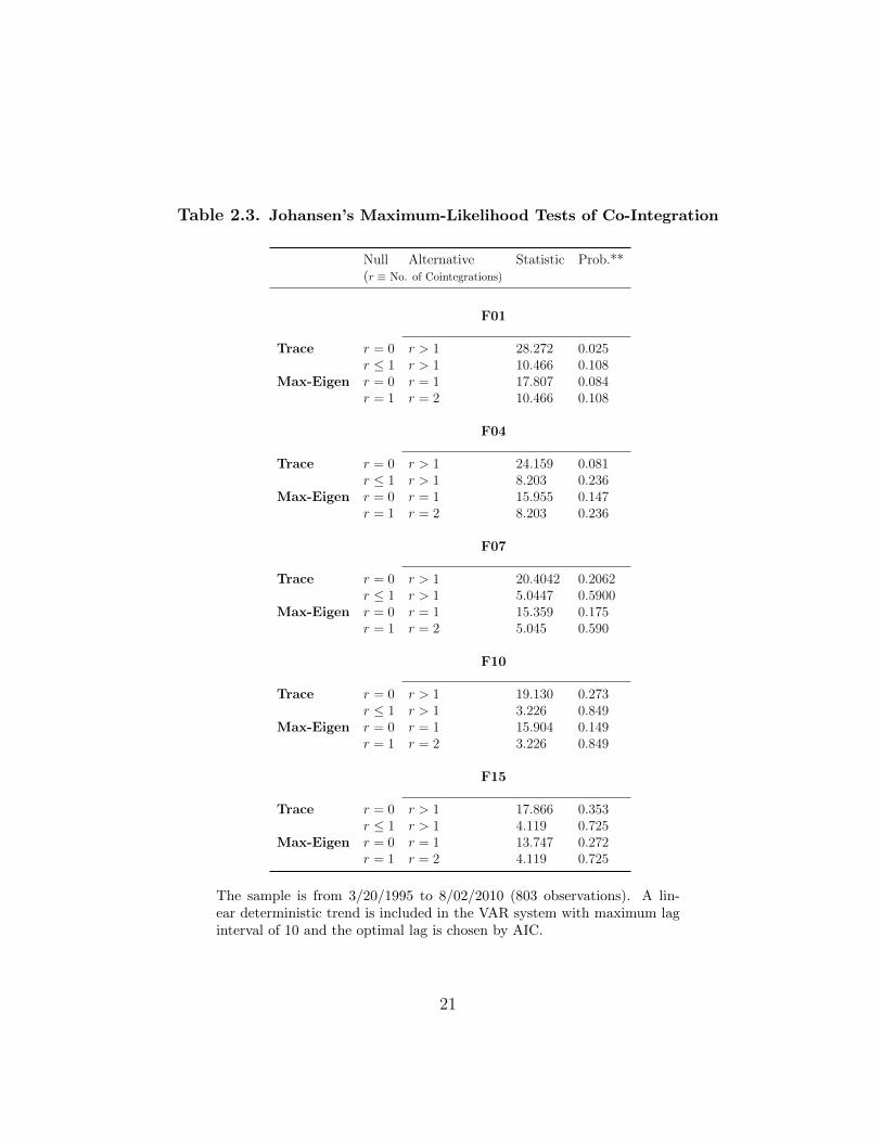
Table 2.3. Johansen’s Maximum-Likelihood Tests of Co-Integration
Null Alternative Statistic Prob.**(r ≡ No. of Cointegrations)
F01
Trace r = 0 r > 1 28.272 0.025r ≤ 1 r > 1 10.466 0.108
Max-Eigen r = 0 r = 1 17.807 0.084r = 1 r = 2 10.466 0.108
F04
Trace r = 0 r > 1 24.159 0.081r ≤ 1 r > 1 8.203 0.236
Max-Eigen r = 0 r = 1 15.955 0.147r = 1 r = 2 8.203 0.236
F07
Trace r = 0 r > 1 20.4042 0.2062r ≤ 1 r > 1 5.0447 0.5900
Max-Eigen r = 0 r = 1 15.359 0.175r = 1 r = 2 5.045 0.590
F10
Trace r = 0 r > 1 19.130 0.273r ≤ 1 r > 1 3.226 0.849
Max-Eigen r = 0 r = 1 15.904 0.149r = 1 r = 2 3.226 0.849
F15
Trace r = 0 r > 1 17.866 0.353r ≤ 1 r > 1 4.119 0.725
Max-Eigen r = 0 r = 1 13.747 0.272r = 1 r = 2 4.119 0.725
The sample is from 3/20/1995 to 8/02/2010 (803 observations). A lin-ear deterministic trend is included in the VAR system with maximum laginterval of 10 and the optimal lag is chosen by AIC.
21

into three components as following12:
Log(Si,t) = Xi,t + xi,t + gi(t), i = 1, 2, (2.1)
where:
Xi,t is a non-stationary stochastic process corresponding to the long-run
movement in the price of commodity i,
xi,t is a mean-reverting stochastic process. It accounts for the short-term
variations in the price of commodity i around its long-run component,
and
gi(t) is a deterministic function corresponding to the seasonal movement in
the price of commodity i. It will be specified later.
In specifying the stochastic behavior of the long-run and the short-run components,
two specifications are considered. I will denote them as Model I and Model II respectively.
Model I
In this model, the behavior of the long-run and the short-run stochastic components,
Xi,t and xi,t respectively, is given by the the following stochastic differential equations
under the physical measure:
12 Given this choice of modeling, the oil price behavior becomes exogenous to the oil sand industry. Thisis not unreasonable because the impact of oil extraction from oil sands on the price of oil is negligible. Oilprices have been increasing recently even with the rise of the supply from oil sands industry, which reflectsthe fact that oil sands supply is not yet to affect on oil prices.
22

Log(Si,t) = Xi,t + xi,t + gi(t), i=1,2,
dX1,t = µ1dt+ σ1dW1,t
dX2,t = µ2dt+ σ2dW2,t
dx1,t = −κ1x1,tdt+ γ1dZ1,t
dx2,t = −κ2x2,tdt+ γ2dZ2,t.
(2.2)
where µi denotes the rate of growth of the long-run component of commodity i, σi denotes
the volatility of the long-run component of the price of commodity i, κi denotes the speed
of mean reversion in the short-run component of the price of commodity i, γi denotes the
volatility of the short-run component of the price of commodity i, and dWi,t and dZi,t are
four possibly correlated increments of Brownian motions.
The system can be written in the following matrix form:
dYt = (M + ΨYt)dt+ ΣdBt, (2.3)
where:
Yt =
X1
X2
x1
x2
, M =
µ1
µ2
0
0
, Ψ =
0 0 0 0
0 0 0 0
0 0 −κ1 0
0 0 0 −κ2
, Σ =
σ1 0 0 0
0 σ2 0 0
0 0 γ1 0
0 0 0 γ2
and
23

Bt =
W1,t
W2,t
Z1,t
Z2,t
.
In this model, the co-movement between the two commodity prices is only captured
through the correlation structure of the Brownian motions increments.
Model II
In this model, motivated by the rule of thumb used in the natural gas market, we let
the long-run component of the natural gas price depend on its deviation from the long-run
component of the crude oil price as follows:
Log(Si,t) = Xi,t + xi,t + gi(t), i = 1, 2,
dX1,t = µ1dt+ σ1dW1,t
dX2,t = α(X1,t −X2,t − χ)dt+ σ2dW2,t
dx1,t = −κ1x1,tdt+ γ1dZ1,t
dx2,t = −κ2x2,tdt+ γ2dZ2,t
(2.4)
In this specification, the long-run component of natural gas reverts to a level of e−χ
from the long-run component of crude oil price. The parameter χ dictates the equilibrium
24
ratio between the two long-run prices. That is, in equilibrium, S2,t = e−χ ·S1,t. Temporary
deviation from this long-run ratio (because of demand and supply imbalances caused by
macro-economic factors and inventory shocks, etc.) will be corrected over the long-run.
Note that the long-run component of oil price, X1,t, is assumed not to depend on the
price of natural gas. This reflects the empirical result that crude oil prices are determined
internationally while natural gas prices are determined regionally (see Villar and Joutz
(2006) and Mohammadi (2009)).
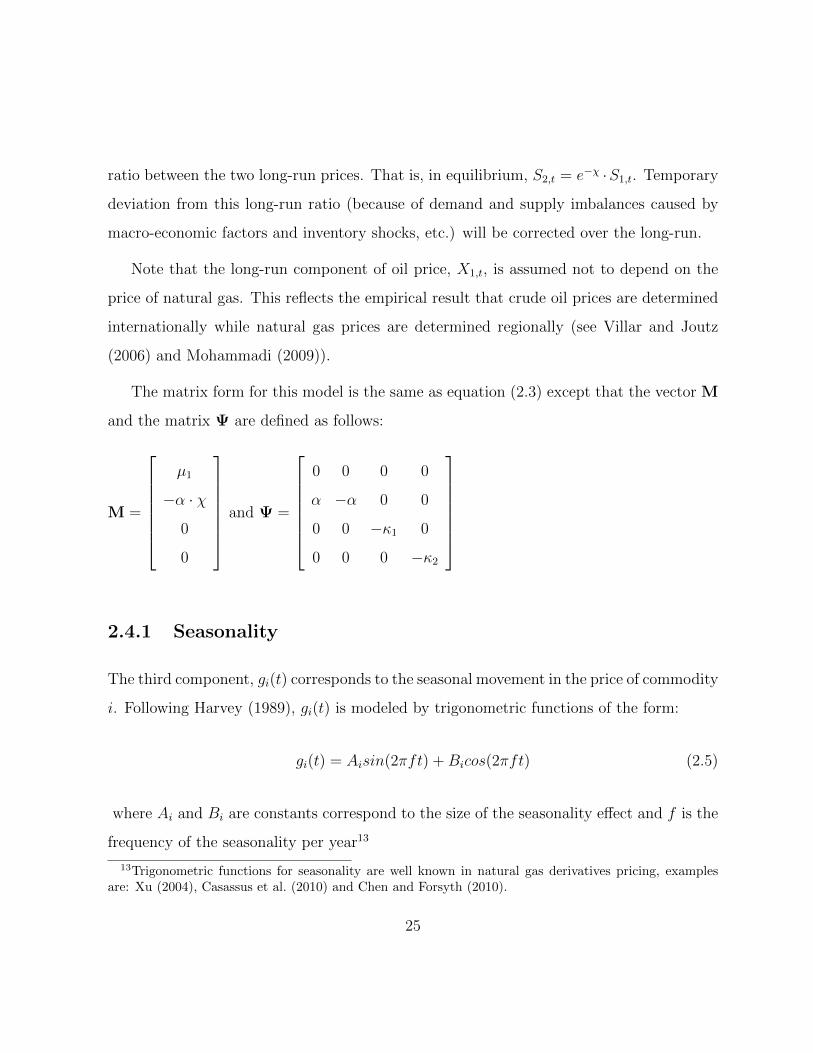
The matrix form for this model is the same as equation (2.3) except that the vector M
and the matrix Ψ are defined as follows:
M =
µ1
−α · χ
0
0
and Ψ =
0 0 0 0
α −α 0 0
0 0 −κ1 0
0 0 0 −κ2
2.4.1 Seasonality
The third component, gi(t) corresponds to the seasonal movement in the price of commodity
i. Following Harvey (1989), gi(t) is modeled by trigonometric functions of the form:
gi(t) = Aisin(2πft) +Bicos(2πft) (2.5)
where Ai and Bi are constants correspond to the size of the seasonality effect and f is the
frequency of the seasonality per year13
13Trigonometric functions for seasonality are well known in natural gas derivatives pricing, examplesare: Xu (2004), Casassus et al. (2010) and Chen and Forsyth (2010).
25
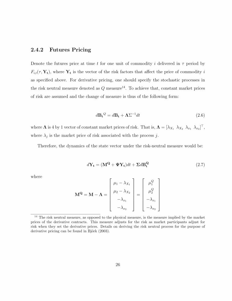
2.4.2 Futures Pricing
Denote the futures price at time t for one unit of commodity i delivered in τ period by
Fi,t(τ,Yt), where Yt is the vector of the risk factors that affect the price of commodity i
as specified above. For derivative pricing, one should specify the stochastic processes in
the risk neutral measure denoted as Q measure14. To achieve that, constant market prices
of risk are assumed and the change of measure is thus of the following form:
dBtQ = dBt + ΛΣ−1dt (2.6)
where Λ is 4 by 1 vector of constant market prices of risk. That is, Λ = [λX1 λX2 λx1 λx2 ]>,
where λj is the market price of risk associated with the process j.
Therefore, the dynamics of the state vector under the risk-neutral measure would be:
dYt = (MQ + ΨYt)dt+ ΣdBQt (2.7)
where
MQ = M−Λ =
µ1 − λX1
µ2 − λX2
−λx1−λx2
=
µQ1
µQ2
−λx1−λx2
14 The risk neutral measure, as opposed to the physical measure, is the measure implied by the market
prices of the derivative contracts. This measure adjusts for the risk as market participants adjust forrisk when they set the derivative prices. Details on deriving the risk neutral process for the purpose ofderivative pricing can be found in Bjork (2003).
26
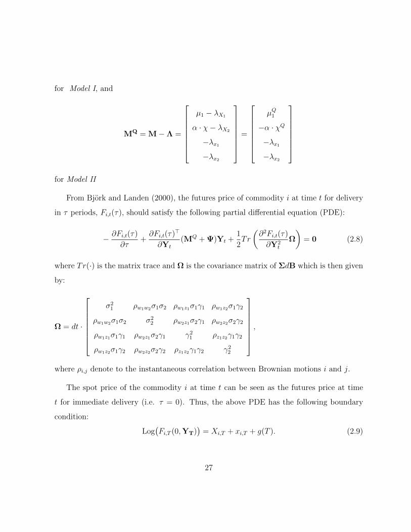
for Model I, and
MQ = M−Λ =
µ1 − λX1
α · χ− λX2
−λx1−λx2
=
µQ1
−α · χQ
−λx1−λx2
for Model II
From Bjork and Landen (2000), the futures price of commodity i at time t for delivery
in τ periods, Fi,t(τ), should satisfy the following partial differential equation (PDE):
− ∂Fi,t(τ)
∂τ+∂Fi,t(τ)>
∂Yt
(MQ + Ψ)Yt +1
2Tr
(∂2Fi,t(τ)
∂Y2t
Ω
)= 0 (2.8)
where Tr(·) is the matrix trace and Ω is the covariance matrix of ΣdB which is then given
by:
Ω = dt ·
σ2
1 ρw1w2σ1σ2 ρw1z1σ1γ1 ρw1z2σ1γ2
ρw1w2σ1σ2 σ22 ρw2z1σ2γ1 ρw2z2σ2γ2
ρw1z1σ1γ1 ρw2z1σ2γ1 γ21 ρz1z2γ1γ2
ρw1z2σ1γ2 ρw2z2σ2γ2 ρz1z2γ1γ2 γ22
,
where ρi,j denote to the instantaneous correlation between Brownian motions i and j.
The spot price of the commodity i at time t can be seen as the futures price at time
t for immediate delivery (i.e. τ = 0). Thus, the above PDE has the following boundary
condition:
Log(Fi,T (0,YT)
)= Xi,T + xi,T + g(T ). (2.9)
27

Since the two models are in the affine framework, the solution of the above PDE has
the following form as shown by Dai and Singleton (2000) and Tian (2003):
Log(Fi,t(τ,Yt
)) = αi(t, τ) + βi(t, τ)Yt, (2.10)
where α(t, τ) and β(t, τ) solve the following system of ordinary differential equations:
− ∂αi(t, τ)
∂τ+ βi(t, τ)MQ +
1
2β(t, τ)Ωβ(t, τ)> = 0 (2.11)
∂β(t, τ)
∂τ− β(t, τ)Ψ = 0, (2.12)
with boundary conditions:
αi(T, 0) = gi(T ) (2.13)
βi(T, 0) = [1 0 1 0] if i = 1 (2.14)
= [0 1 0 1] if i = 2. (2.15)
Integrating (2.12) and then plug it into (2.11), one gets:
βi(t, τ) = βi(T, 0)e(Ψτ) (2.16)
αi(t, τ) = gi(T ) +
∫ τ
0
(βi(t, u)MQ +
1
2β(t, u)Ωβ(t, u)>
)du. (2.17)
Thus, the futures prices for Model I is given by:
Log(Fi,t(τ)) = gi(T ) +Xi + xieκiτ + µQi τ +
1
2σ2i τ
+
(λxiκi− σiγiρwizi
κi
)(e−κiτ − 1
)− γ2
i
4κi(e−2κiτ − 1), (2.18)
28
where i = 1, 2.
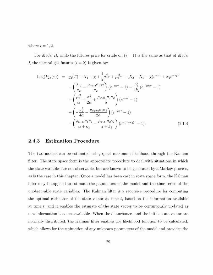
For Model II, while the futures price for crude oil (i = 1) is the same as that of Model
I, the natural gas futures (i = 2) is given by:
Log(F2,t(τ)) = g2(T ) +X1 + χ+1
2σ2
1τ + µQ1 τ + (X2 −X1 − χ)e−ατ + x2e−κ2τ
+
(λx2κ2
− ρw1z2σ1γ2
κ2
)(e−κ2τ − 1
)− γ2
2
4k2
(e−2k2τ − 1)
+
(µQ1α
+σ2
1
2α+ρw1w2σ1σ2
α
)(e−ατ − 1)
+
(−σ
22
4α− ρw1w2σ1σ2
2α
)(e−2ατ − 1)
+
(ρw1z2σ1γ2
α + κ2
− ρw2z2σ2γ2
α + k2
)(e−(α+κ2)τ − 1). (2.19)
2.4.3 Estimation Procedure
The two models can be estimated using quasi maximum likelihood through the Kalman
filter. The state space form is the appropriate procedure to deal with situations in which
the state variables are not observable, but are known to be generated by a Markov process,
as is the case in this chapter. Once a model has been cast in state space form, the Kalman
filter may be applied to estimate the parameters of the model and the time series of the
unobservable state variables. The Kalman filter is a recursive procedure for computing
the optimal estimator of the state vector at time t, based on the information available
at time t, and it enables the estimate of the state vector to be continuously updated as
new information becomes available. When the disturbances and the initial state vector are
normally distributed, the Kalman filter enables the likelihood function to be calculated,
which allows for the estimation of any unknown parameters of the model and provides the
29
basis for statistical testing and model specification. For a detailed discussion of state space
models and the Kalman filter see Chapter 3 in Harvey (1989).
To cast the models in the state space form, one needs to specify the transition equation
that governs the dynamic of the state variables and the measurement equation that relates
the observable variables to the state variables.
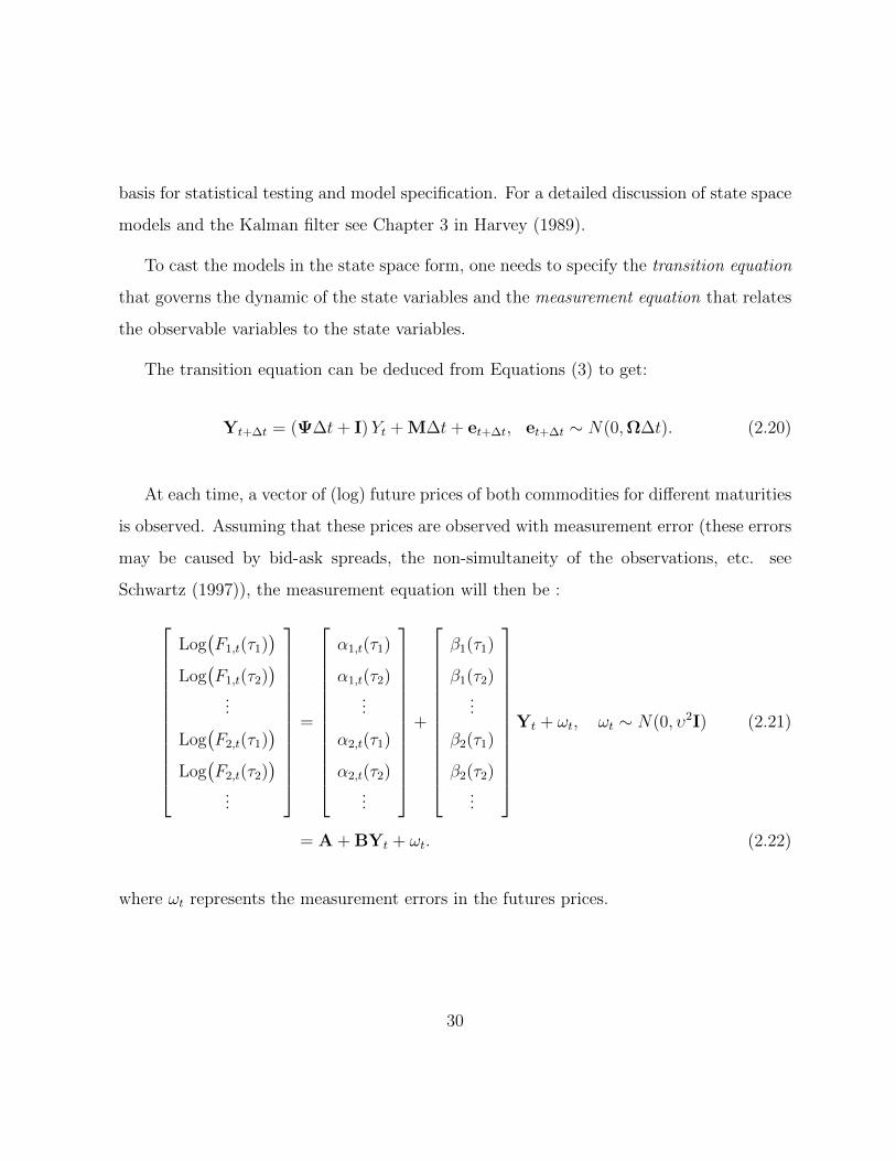
The transition equation can be deduced from Equations (3) to get:
Yt+∆t = (Ψ∆t+ I)Yt + M∆t+ et+∆t, et+∆t ∼ N(0,Ω∆t). (2.20)
At each time, a vector of (log) future prices of both commodities for different maturities
is observed. Assuming that these prices are observed with measurement error (these errors
may be caused by bid-ask spreads, the non-simultaneity of the observations, etc. see
Schwartz (1997)), the measurement equation will then be :
Log(F1,t(τ1)
)Log
(F1,t(τ2)
)...
Log(F2,t(τ1)
)Log
(F2,t(τ2)
)...
=
α1,t(τ1)
α1,t(τ2)...
α2,t(τ1)
α2,t(τ2)...
+
β1(τ1)
β1(τ2)...
β2(τ1)
β2(τ2)...
Yt + ωt, ωt ∼ N(0, υ2I) (2.21)
= A + BYt + ωt. (2.22)
where ωt represents the measurement errors in the futures prices.
30

2.5 Oil Sands Valuation Model
In this section, Brennan and Schwartz (1985) modeling procedure is extended to account
for a stochastic extraction cost. Consider a competitive firm that operates an oil sands
project to extract bitumen from known inventory of Q units. The project is assumed to
be currently operating which means that initial cost to build the facility is sunk.
When the project is operating, the profit flow rate generated by selling the produced
amount from t to t+ dt is given by:
Πt = qt(St − c1 − vt
)− c2 − τax, (2.23)
where qt is the optimal rate of production in barrels per unit of time which is assumed to
be known to the management, St is the price of one barrel of bitumen, c1 is a deterministic
variable cost, vt is a stochastic variable cost, c2 is the fixed cost and τax is the total taxes
consisting of income tax plus royalties.
Since most bitumen is upgraded to crude oil, the dynamic of the bitumen price will
imitate the dynamic of the crude oil price. Thus, the dynamic of St is given by the dynamic
of S1,t specified in section 2.4.
In the case of the oil sands industry, vt corresponds mainly to the cost of natural gas
purchases in order to produce one unit of bitumen. Thus, vt is governed by the dynamics
of S2,t specified in section 2.4.
Depending on profitability, the decision-maker has the option to switch between differ-
ent modes of operation. When the price drops low enough, the decision-maker can incur a
fixed cost, Koc, and suspend the operation until the price level goes back up to profitable
levels. During suspension, the decision-maker should also incur a flow of maintenance cost,
31

M. If the price drops dramatically to very low levels, the decision-maker has the option
to abandon the project permanently. On the other hand, if the project is currently closed
and the price recovers to a profitable level, the decision-maker has the option to reopen
the field again by paying another fixed cost of Kco. These options have value and option
pricing theory can be used to find their values. Since the options are of the American
type, their values are the the sum of all expected future cash flows from pursuing the
optimal exercise policy discounted at the risk-free rate. The above project can be seen as
an American option where the underlying assets are the price of crude oil and natural gas
modeled in the last section. Thus, the value of the project is the sum of all expected future
cash flows discounted at the risk free rate, provided that the optimal policy of switching
between operation modes is pursued.
For a small time step of ∆t, the value of the project is then be governed by the following
two Bellman equations for currently open and closed projects respectively15:
Vopen
(Yt, Q, t
)=
max
Πt∆t+ e−(r+τo)∆tEt
[Vopen(Yt+∆t, Q− q∆t, t+ ∆t)
]open
−M∆t−Koc + e−(r+τc)∆tEt[Vclosed(Yt+∆t, Q, t+ ∆t)
]close
0 abandon
(2.24)
Vclosed
(Yt, Q, t
)=
max
Πt∆t−Kco + e−(r+τo)∆tEt
[Vopen(Yt+∆t, Q− q∆t, t+ ∆t)
]re-open
−M∆t+ e−(r+τc)∆tEt[Vclosed(Yt+∆t, Q, t+ ∆t)
]close
0 abandon,
(2.25)
15In continuous time, and given that the prices are modeled without jumps, an open project can not beabandoned directly without being temporary closed. Thus, in continuous time setting, the third line inequation 2.24 should be dropped.
32
where τi , i = o or c, is the property tax rate proportional to project value when it is
open and when it is closed respectively. r is the risk free rate. As mentioned above, the
expectations are taken under the risk-neutral measure.
Analytical solutions to equations (2.24) and (2.25) are unavailable, thus numerical
methods should be used. Several numerical methods have been proposed for such problem.
Among them are: finite difference and lattice methods. The Least Square Monte Carlo
(LSMC) method developed by Longstaff and Schwartz (2001) has proved to be an efficient
and simple tool for such problems (see Cortazar et al. (2008) and Tsekrekos et al. (2010)).
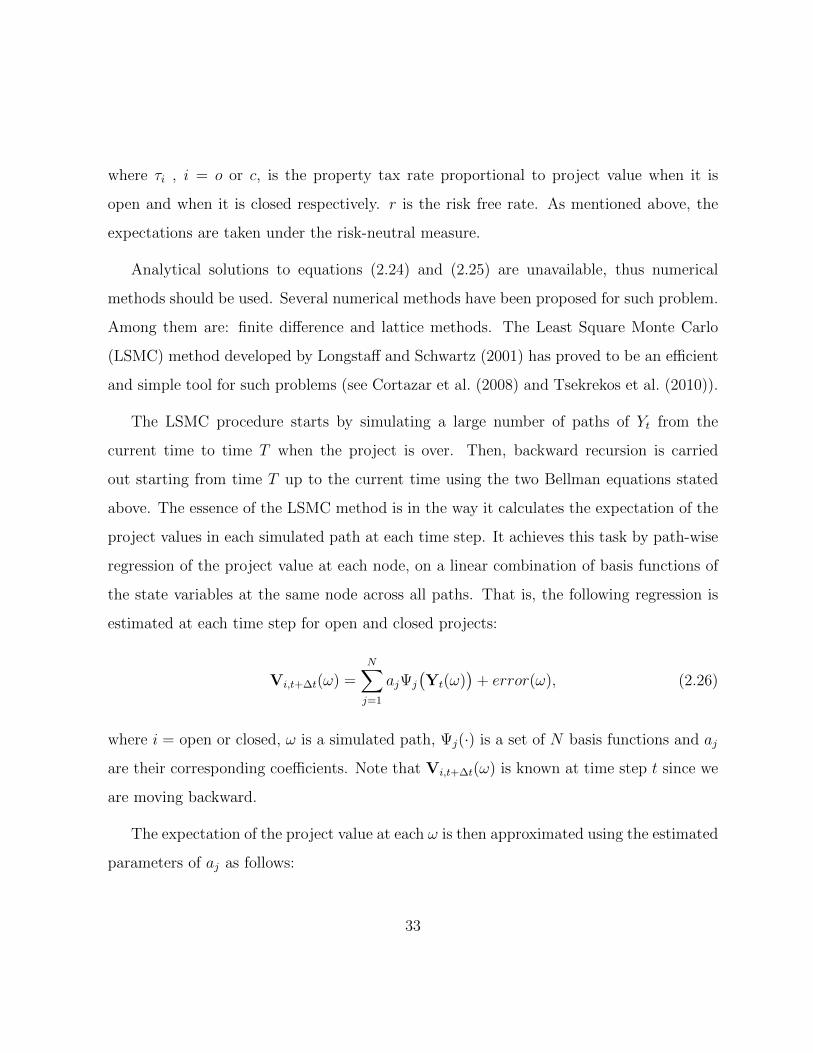
The LSMC procedure starts by simulating a large number of paths of Yt from the
current time to time T when the project is over. Then, backward recursion is carried
out starting from time T up to the current time using the two Bellman equations stated
above. The essence of the LSMC method is in the way it calculates the expectation of the
project values in each simulated path at each time step. It achieves this task by path-wise
regression of the project value at each node, on a linear combination of basis functions of
the state variables at the same node across all paths. That is, the following regression is
estimated at each time step for open and closed projects:
Vi,t+∆t(ω) =N∑j=1
ajΨj
(Yt(ω)
)+ error(ω), (2.26)
where i = open or closed, ω is a simulated path, Ψj(·) is a set of N basis functions and aj
are their corresponding coefficients. Note that Vi,t+∆t(ω) is known at time step t since we
are moving backward.
The expectation of the project value at each ω is then approximated using the estimated
parameters of aj as follows:
33
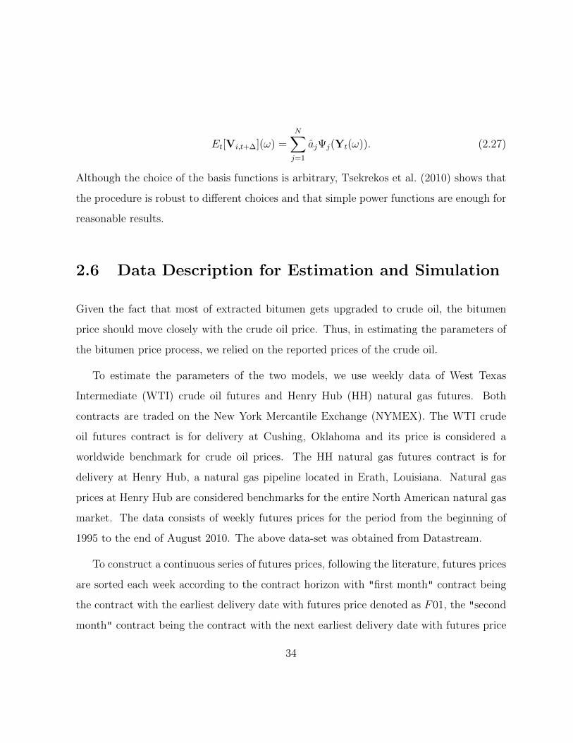
Et[Vi,t+∆](ω) =N∑j=1
ajΨj(Yt(ω)). (2.27)
Although the choice of the basis functions is arbitrary, Tsekrekos et al. (2010) shows that
the procedure is robust to different choices and that simple power functions are enough for
reasonable results.
2.6 Data Description for Estimation and Simulation
Given the fact that most of extracted bitumen gets upgraded to crude oil, the bitumen
price should move closely with the crude oil price. Thus, in estimating the parameters of
the bitumen price process, we relied on the reported prices of the crude oil.
To estimate the parameters of the two models, we use weekly data of West Texas
Intermediate (WTI) crude oil futures and Henry Hub (HH) natural gas futures. Both
contracts are traded on the New York Mercantile Exchange (NYMEX). The WTI crude
oil futures contract is for delivery at Cushing, Oklahoma and its price is considered a
worldwide benchmark for crude oil prices. The HH natural gas futures contract is for
delivery at Henry Hub, a natural gas pipeline located in Erath, Louisiana. Natural gas
prices at Henry Hub are considered benchmarks for the entire North American natural gas
market. The data consists of weekly futures prices for the period from the beginning of
1995 to the end of August 2010. The above data-set was obtained from Datastream.
To construct a continuous series of futures prices, following the literature, futures prices
are sorted each week according to the contract horizon with "first month" contract being
the contract with the earliest delivery date with futures price denoted as F01, the "second
month" contract being the contract with the next earliest delivery date with futures price
34
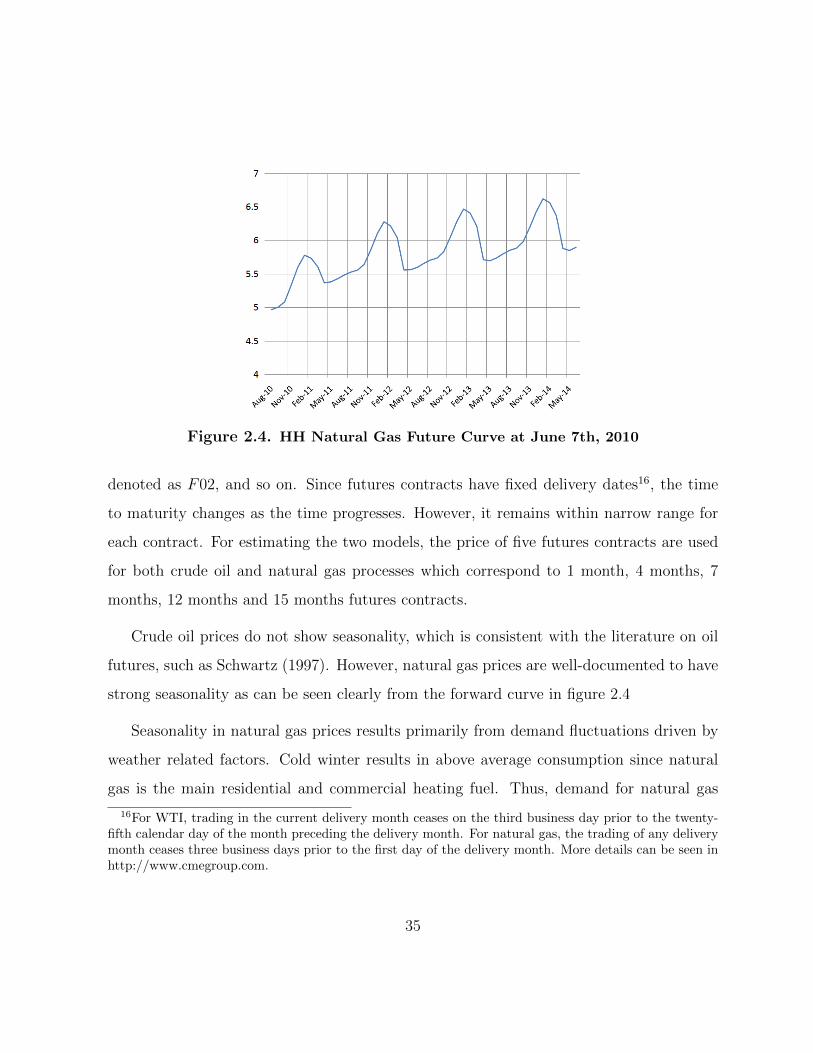
Figure 2.4. HH Natural Gas Future Curve at June 7th, 2010
denoted as F02, and so on. Since futures contracts have fixed delivery dates16, the time
to maturity changes as the time progresses. However, it remains within narrow range for
each contract. For estimating the two models, the price of five futures contracts are used
for both crude oil and natural gas processes which correspond to 1 month, 4 months, 7
months, 12 months and 15 months futures contracts.
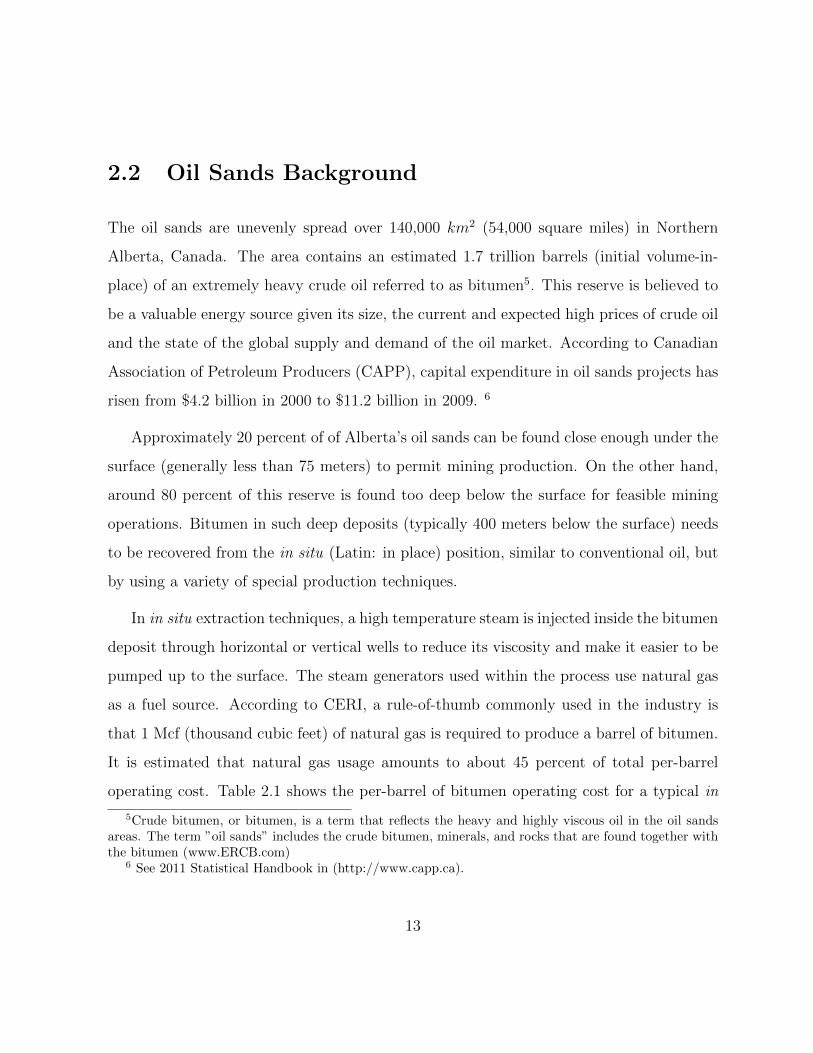
Crude oil prices do not show seasonality, which is consistent with the literature on oil
futures, such as Schwartz (1997). However, natural gas prices are well-documented to have
strong seasonality as can be seen clearly from the forward curve in figure 2.4
Seasonality in natural gas prices results primarily from demand fluctuations driven by
weather related factors. Cold winter results in above average consumption since natural
gas is the main residential and commercial heating fuel. Thus, demand for natural gas
16For WTI, trading in the current delivery month ceases on the third business day prior to the twenty-fifth calendar day of the month preceding the delivery month. For natural gas, the trading of any deliverymonth ceases three business days prior to the first day of the delivery month. More details can be seen inhttp://www.cmegroup.com.
35
is typically high in winter and since storage facilities are limited, winter-maturing futures
tend to be higher than those maturing in summer as is clear from figure 2.4. Since the
seasonality is yearly, f in equation (2.5) is set equal to 1. For more details on the seasonal
behavior of gas prices, see Xu (2004).
To accomplish the objective of this study, a hypothetical in situ oil sands project with a
capacity of 5 million barrel per year is considered 17. The decision-maker, for simplicity, is
assumed to have four opportunities per year to switch between operating modes18. In the
CERI 2009 report about supply cost in oil sands19, variable cost is assumed to be $6.8 per
barrel, which is our estimate for c1. In the same report, for a capacity of 30,000 barrels per
day, the report estimated the annual average of the capital cost (excluding the initial cost
of building the facility) to be 36.5 million dollars and the fixed operation costs to be 61.2
million dollars. Dividing the sum by the capacity assumed in the report and multiplying
the result by $5 millions barrel per year, the capacity assumed in this study, we get $41
millions per year of fixed cost, our estimate for c2. Maintaining the project while closed is
assumed to be 10% of the fixed operating cost which is going to be around $4 million per
year. For simplicity, switching costs are assumed to be zero, i.e. the operator can switch
to closed mode without incurring a cost. This implies that the value of the project is the
same whether it is open or suspended as it is clear from the two bellman equations. The
impact of switching costs on the value of a natural resource has been studied in Mason
17 This choice coincides with some of the existing projects, see CERI 2008 report. Higher projectcapacities also exist, but considering them will be at the cost of the speed of simulation without muchimpact on the nature of the results.
18 This assumption is used to make the size of the numerical calculation manageable. Increasing theswitching opportunities frequency will increase the size of the working matrices exponentially. It certainlymakes the values to be more precise but will not change the pattern of the results. This assumption hasshown up in literature as well, for example: Cortazar et al. (2008) assumed only 3 opportunities to switch.
19See Table 3.1 in: McColl, Mei, Millington and Slagorsky ”Canadian Oil Sands Supply Costs andDevelopment Projects (2009-2043)” Canadian Energy Research Institute, November 2009
36
(2001)20.
For tax parameters, CERI 2009 report assumption of constant income tax at nineteen
percent (federal) and ten percent (provincial) is assumed. The royalties system of the oil
sand industry relates the applicable royalties to the price of WTI crude oil and whether
the project has reached its payout. Project payout would be said to have occurred when
accumulated revenues first exceeded accumulated capital and operating expenditures. The
rule is to apply a base royalties of 1% if WTI ≤ $55, 9% if WTI ≥ $120 with linear
interpolation when WTI is in between until the project payout; thereafter, the royalties
will be the greater of the base royalty or a net revenue royalty of 25% if WTI≤ $55
and 40% if WTI ≥ $120 with linear interpolation when WTI is in between. To avoid
adding additional state variables, we assume that the project is past the payout. Property
tax is applied to the oil sands project at a rate of 1%. More details can be found in
http://www.energy.alberta.ca. Finally, I follow CERI report in applying 2.5% rate of
inflation. This rate of inflation is applied to the deterministic variable and fixed costs (c1
and C2) and the maintenance cost (M). Table 2.4 summaries these parameter that are
used in simulation.
2.7 Results
Table 2.5 shows main descriptive statistics for the (log) returns of different futures prices of
different delivery months for both commodities. It is clear from the table that the natural
gas returns exhibit higher volatility than crude oil returns. The natural gas market is more
sensitive to fluctuating factors such as inventory and weather related factors. Volatility of
20As Mason (2001) shows, greater switching costs cause firms to be less inclined to change status.However, non-zero switching costs will not change the way the project value and the optimal switchingprices react to the dynamic of natural gas prices, the main focus of the paper.
37
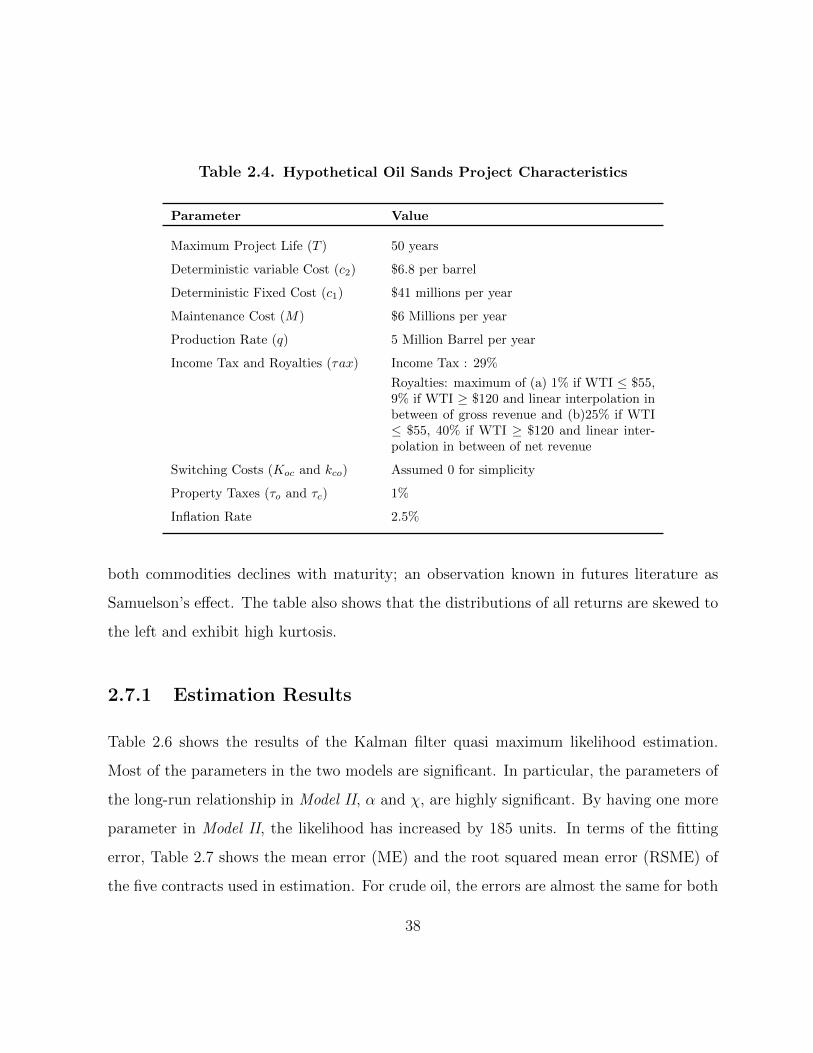
Table 2.4. Hypothetical Oil Sands Project Characteristics
Parameter Value
Maximum Project Life (T ) 50 years
Deterministic variable Cost (c2) $6.8 per barrel
Deterministic Fixed Cost (c1) $41 millions per year
Maintenance Cost (M) $6 Millions per year
Production Rate (q) 5 Million Barrel per year
Income Tax and Royalties (τax) Income Tax : 29%
Royalties: maximum of (a) 1% if WTI ≤ $55,9% if WTI ≥ $120 and linear interpolation inbetween of gross revenue and (b)25% if WTI≤ $55, 40% if WTI ≥ $120 and linear inter-polation in between of net revenue
Switching Costs (Koc and kco) Assumed 0 for simplicity
Property Taxes (τo and τc) 1%
Inflation Rate 2.5%
both commodities declines with maturity; an observation known in futures literature as
Samuelson’s effect. The table also shows that the distributions of all returns are skewed to
the left and exhibit high kurtosis.
2.7.1 Estimation Results
Table 2.6 shows the results of the Kalman filter quasi maximum likelihood estimation.
Most of the parameters in the two models are significant. In particular, the parameters of
the long-run relationship in Model II, α and χ, are highly significant. By having one more
parameter in Model II, the likelihood has increased by 185 units. In terms of the fitting
error, Table 2.7 shows the mean error (ME) and the root squared mean error (RSME) of
the five contracts used in estimation. For crude oil, the errors are almost the same for both
38
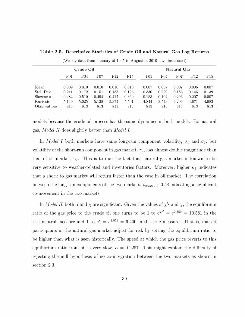
Table 2.5. Descriptive Statistics of Crude Oil and Natural Gas Log Returns
(Weekly data from January of 1995 to August of 2010 have been used)
Crude Oil Natural Gas
F01 F04 F07 F12 F15 F01 F04 F07 F12 F15
Mean 0.009 0.010 0.010 0.010 0.010 0.007 0.007 0.007 0.006 0.007Std. Dev. 0.211 0.172 0.151 0.133 0.126 0.330 0.229 0.183 0.145 0.139Skewness -0.482 -0.510 -0.494 -0.417 -0.360 0.183 -0.104 -0.296 -0.207 -0.507Kurtosis 5.149 5.025 5.128 5.374 5.501 4.844 3.543 4.296 4.671 4.983Observations 813 813 813 813 813 813 813 813 813 813
models because the crude oil process has the same dynamics in both models. For natural
gas, Model II does slightly better than Model I.
In Model I both markets have same long-run component volatility, σ1 and σ2, but
volatility of the short-run component in gas market, γ2, has almost double magnitude than
that of oil market, γ1. This is to due the fact that natural gas market is known to be
very sensitive to weather-related and inventories factors. Moreover, higher κ2 indicates
that a shock to gas market will return faster than the case in oil market. The correlation
between the long-run components of the two markets, ρw1w2 , is 0.48 indicating a significant
co-movement in the two markets.
In Model II, both α and χ are significant. Given the values of χQ and χ, the equilibrium
ratio of the gas price to the crude oil one turns to be 1 to eχQ
= e2.359 = 10.581 in the
risk neutral measure and 1 to eχ = e1.853 = 6.400 in the true measure. That is, market
participants in the natural gas market adjust for risk by setting the equilibrium ratio to
be higher than what is seen historically. The speed at which the gas price reverts to this
equilibrium ratio from oil is very slow, α = 0.2257. This might explain the difficulty of
rejecting the null hypothesis of no co-integration between the two markets as shown in
section 2.3.
39
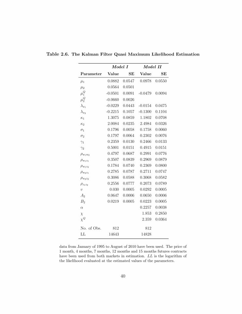
Table 2.6. The Kalman Filter Quasi Maximum Likelihood Estimation
Model I Model II
Parameter Value SE Value SE
µ1 0.0882 0.0547 0.0978 0.0550
µ2 0.0564 0.0501
µQ1 -0.0501 0.0091 -0.0479 0.0094
µQ2 -0.0660 0.0026
λx1 -0.0229 0.0443 -0.0154 0.0475
λx2 -0.2215 0.1057 -0.1300 0.1104
κ1 1.3075 0.0859 1.1802 0.0708
κ2 2.0084 0.0235 2.4984 0.0326
σ1 0.1796 0.0058 0.1758 0.0060
σ2 0.1797 0.0064 0.2302 0.0076
γ1 0.2359 0.0130 0.2466 0.0133
γ2 0.5001 0.0151 0.4915 0.0151
ρw1w2 0.4797 0.0687 0.2991 0.0776
ρw1z1 0.3507 0.0839 0.2969 0.0879
ρw1z2 0.1784 0.0740 0.2369 0.0800
ρw2z1 0.2785 0.0787 0.2711 0.0747
ρw2z2 0.3086 0.0588 0.3068 0.0582
ρz1z2 0.2556 0.0777 0.2073 0.0789
v 0.030 0.0005 0.0292 0.0005
A2 0.0647 0.0006 0.0650 0.0006
B2 0.0219 0.0005 0.0223 0.0005
α 0.2257 0.0038
χ 1.853 0.2850
χQ 2.359 0.0364
No. of Obs. 812 812
LL 14643 14828
data from January of 1995 to August of 2010 have been used. The price of1 month, 4 months, 7 months, 12 months and 15 months futures contractshave been used from both markets in estimation. LL is the logarithm ofthe likelihood evaluated at the estimated values of the parameters.
40
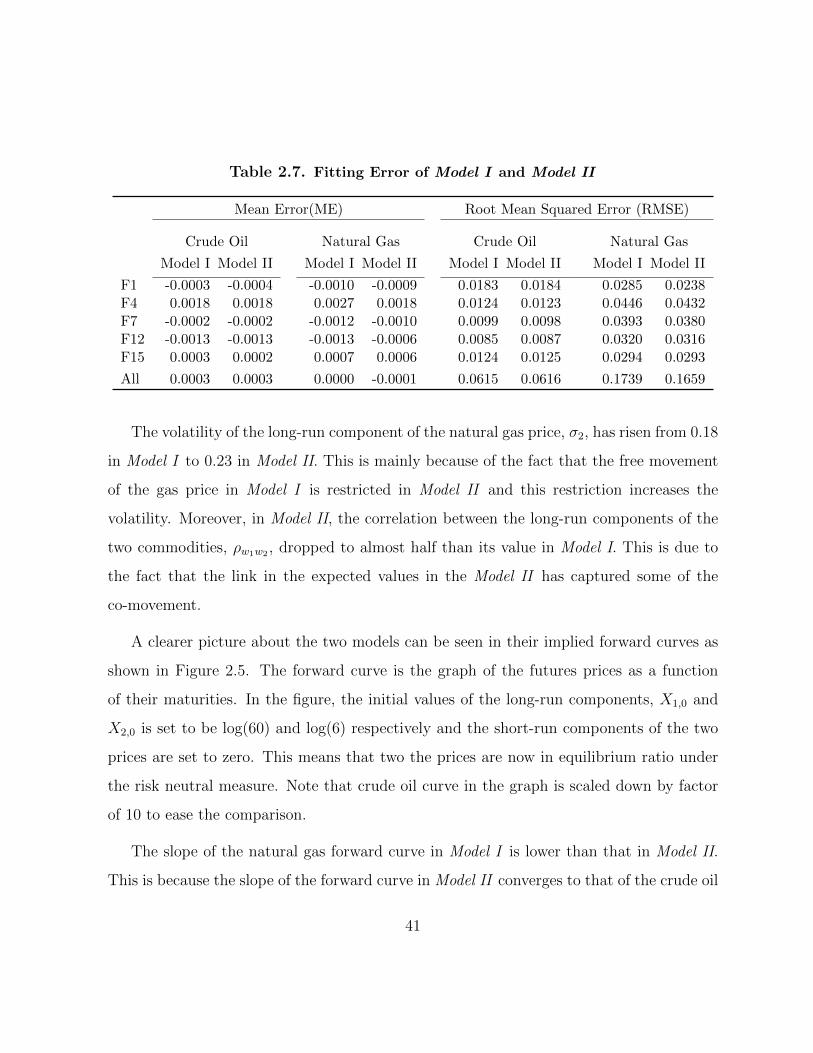
Table 2.7. Fitting Error of Model I and Model II
Mean Error(ME) Root Mean Squared Error (RMSE)
Crude Oil Natural Gas Crude Oil Natural Gas
Model I Model II Model I Model II Model I Model II Model I Model II
F1 -0.0003 -0.0004 -0.0010 -0.0009 0.0183 0.0184 0.0285 0.0238F4 0.0018 0.0018 0.0027 0.0018 0.0124 0.0123 0.0446 0.0432F7 -0.0002 -0.0002 -0.0012 -0.0010 0.0099 0.0098 0.0393 0.0380F12 -0.0013 -0.0013 -0.0013 -0.0006 0.0085 0.0087 0.0320 0.0316F15 0.0003 0.0002 0.0007 0.0006 0.0124 0.0125 0.0294 0.0293
All 0.0003 0.0003 0.0000 -0.0001 0.0615 0.0616 0.1739 0.1659
The volatility of the long-run component of the natural gas price, σ2, has risen from 0.18
in Model I to 0.23 in Model II. This is mainly because of the fact that the free movement
of the gas price in Model I is restricted in Model II and this restriction increases the
volatility. Moreover, in Model II, the correlation between the long-run components of the
two commodities, ρw1w2 , dropped to almost half than its value in Model I. This is due to
the fact that the link in the expected values in the Model II has captured some of the
co-movement.
A clearer picture about the two models can be seen in their implied forward curves as
shown in Figure 2.5. The forward curve is the graph of the futures prices as a function
of their maturities. In the figure, the initial values of the long-run components, X1,0 and
X2,0 is set to be log(60) and log(6) respectively and the short-run components of the two
prices are set to zero. This means that two the prices are now in equilibrium ratio under
the risk neutral measure. Note that crude oil curve in the graph is scaled down by factor
of 10 to ease the comparison.
The slope of the natural gas forward curve in Model I is lower than that in Model II.
This is because the slope of the forward curve in Model II converges to that of the crude oil
41
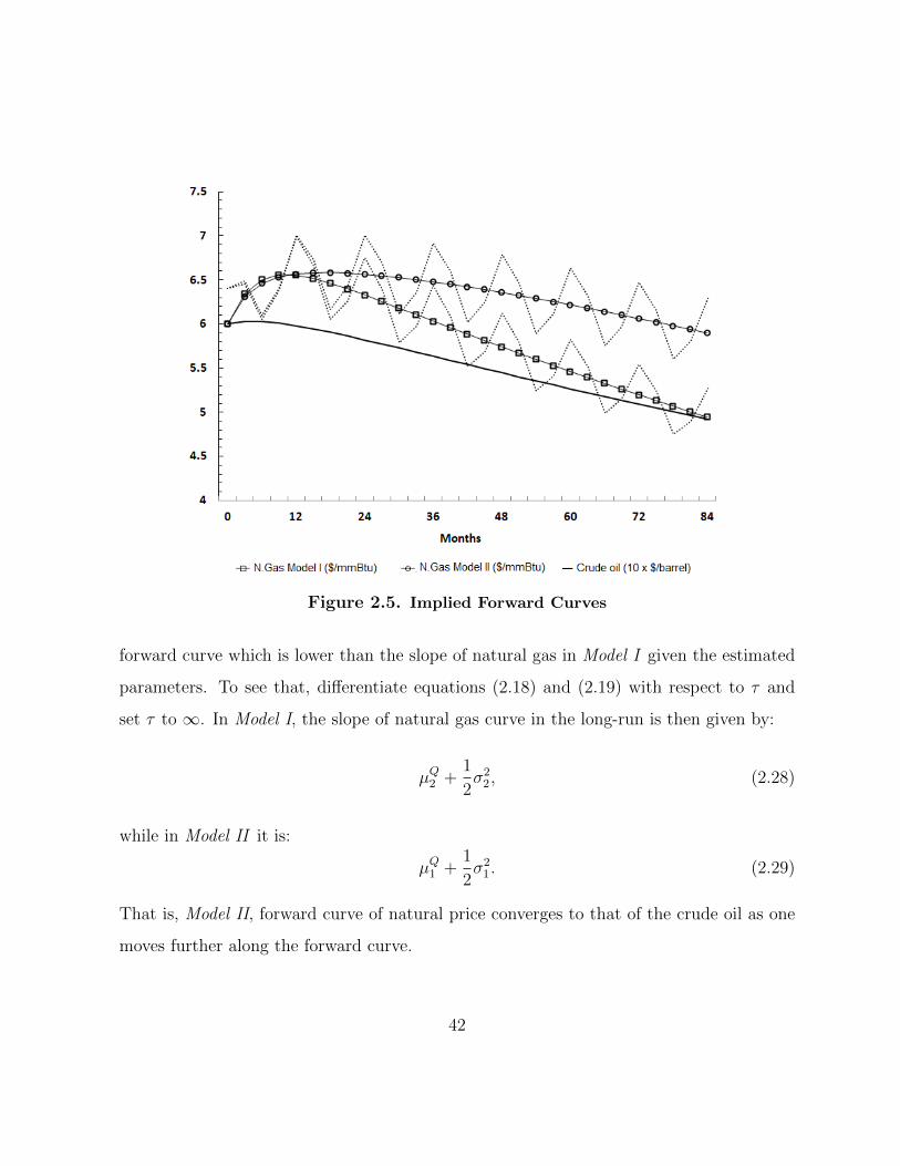
Figure 2.5. Implied Forward Curves
forward curve which is lower than the slope of natural gas in Model I given the estimated
parameters. To see that, differentiate equations (2.18) and (2.19) with respect to τ and
set τ to ∞. In Model I, the slope of natural gas curve in the long-run is then given by:
µQ2 +1
2σ2
2, (2.28)
while in Model II it is:
µQ1 +1
2σ2
1. (2.29)
That is, Model II, forward curve of natural price converges to that of the crude oil as one
moves further along the forward curve.
42
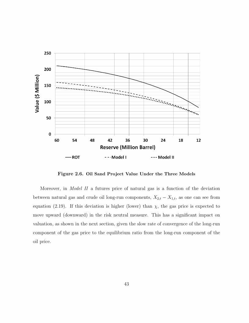
Figure 2.6. Oil Sand Project Value Under the Three Models
Moreover, in Model II a futures price of natural gas is a function of the deviation
between natural gas and crude oil long-run components, X2,t − X1,t, as one can see from
equation (2.19). If this deviation is higher (lower) than χ, the gas price is expected to
move upward (downward) in the risk neutral measure. This has a significant impact on
valuation, as shown in the next section, given the slow rate of convergence of the long-run
component of the gas price to the equilibrium ratio from the long-run component of the
oil price.
43
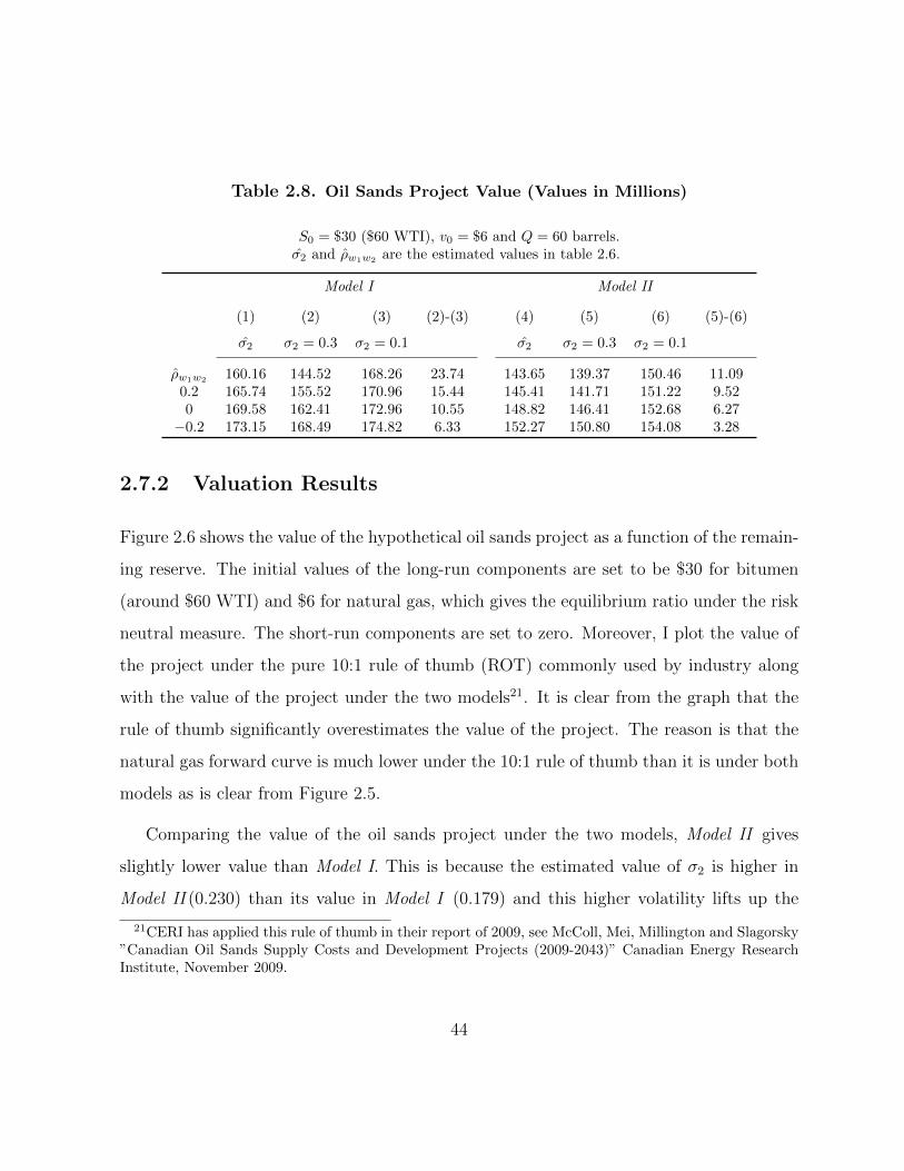
Table 2.8. Oil Sands Project Value (Values in Millions)
S0 = $30 ($60 WTI), v0 = $6 and Q = 60 barrels.σ2 and ρw1w2
are the estimated values in table 2.6.
Model I Model II
(1) (2) (3) (2)-(3) (4) (5) (6) (5)-(6)
σ2 σ2 = 0.3 σ2 = 0.1 σ2 σ2 = 0.3 σ2 = 0.1
ρw1w2160.16 144.52 168.26 23.74 143.65 139.37 150.46 11.09
0.2 165.74 155.52 170.96 15.44 145.41 141.71 151.22 9.520 169.58 162.41 172.96 10.55 148.82 146.41 152.68 6.27−0.2 173.15 168.49 174.82 6.33 152.27 150.80 154.08 3.28
2.7.2 Valuation Results
Figure 2.6 shows the value of the hypothetical oil sands project as a function of the remain-
ing reserve. The initial values of the long-run components are set to be $30 for bitumen
(around $60 WTI) and $6 for natural gas, which gives the equilibrium ratio under the risk
neutral measure. The short-run components are set to zero. Moreover, I plot the value of
the project under the pure 10:1 rule of thumb (ROT) commonly used by industry along
with the value of the project under the two models21. It is clear from the graph that the
rule of thumb significantly overestimates the value of the project. The reason is that the
natural gas forward curve is much lower under the 10:1 rule of thumb than it is under both
models as is clear from Figure 2.5.
Comparing the value of the oil sands project under the two models, Model II gives
slightly lower value than Model I. This is because the estimated value of σ2 is higher in
Model II (0.230) than its value in Model I (0.179) and this higher volatility lifts up the
21CERI has applied this rule of thumb in their report of 2009, see McColl, Mei, Millington and Slagorsky”Canadian Oil Sands Supply Costs and Development Projects (2009-2043)” Canadian Energy ResearchInstitute, November 2009.
44
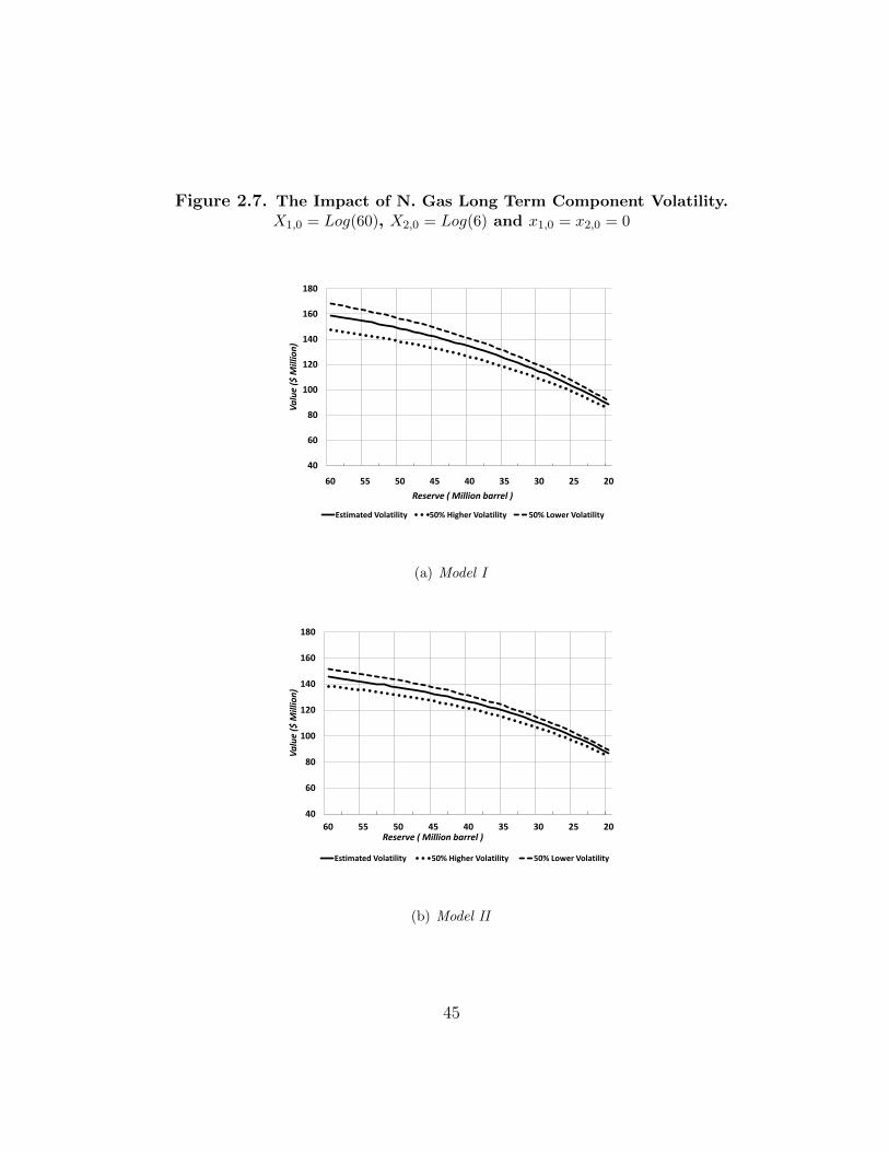
Figure 2.7. The Impact of N. Gas Long Term Component Volatility.X1,0 = Log(60), X2,0 = Log(6) and x1,0 = x2,0 = 0
40
60
80
100
120
140
160
180
60 55 50 45 40 35 30 25 20
Va
lue
($ M
illio
n)
Reserve ( Million barrel )
Estimated Volatility 50% Higher Volatility 50% Lower Volatility
(a) Model I
40
60
80
100
120
140
160
180
60 55 50 45 40 35 30 25 20
Va
lue
($ M
illio
n)
Reserve ( Million barrel )
Estimated Volatility 50% Higher Volatility 50% Lower Volatility
(b) Model II
45
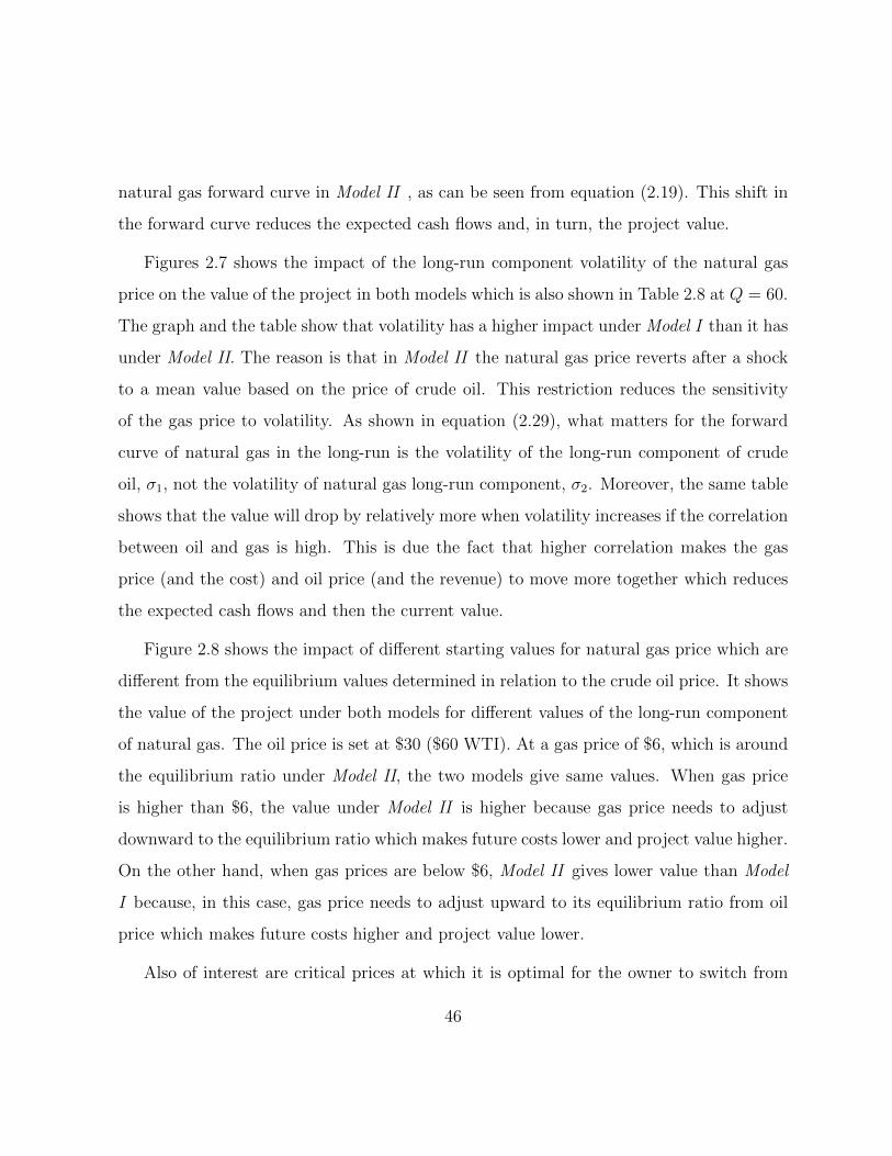
natural gas forward curve in Model II , as can be seen from equation (2.19). This shift in
the forward curve reduces the expected cash flows and, in turn, the project value.
Figures 2.7 shows the impact of the long-run component volatility of the natural gas
price on the value of the project in both models which is also shown in Table 2.8 at Q = 60.
The graph and the table show that volatility has a higher impact under Model I than it has
under Model II. The reason is that in Model II the natural gas price reverts after a shock
to a mean value based on the price of crude oil. This restriction reduces the sensitivity
of the gas price to volatility. As shown in equation (2.29), what matters for the forward
curve of natural gas in the long-run is the volatility of the long-run component of crude
oil, σ1, not the volatility of natural gas long-run component, σ2. Moreover, the same table
shows that the value will drop by relatively more when volatility increases if the correlation
between oil and gas is high. This is due the fact that higher correlation makes the gas
price (and the cost) and oil price (and the revenue) to move more together which reduces
the expected cash flows and then the current value.
Figure 2.8 shows the impact of different starting values for natural gas price which are
different from the equilibrium values determined in relation to the crude oil price. It shows
the value of the project under both models for different values of the long-run component
of natural gas. The oil price is set at $30 ($60 WTI). At a gas price of $6, which is around
the equilibrium ratio under Model II, the two models give same values. When gas price
is higher than $6, the value under Model II is higher because gas price needs to adjust
downward to the equilibrium ratio which makes future costs lower and project value higher.
On the other hand, when gas prices are below $6, Model II gives lower value than Model
I because, in this case, gas price needs to adjust upward to its equilibrium ratio from oil
price which makes future costs higher and project value lower.
Also of interest are critical prices at which it is optimal for the owner to switch from
46

Figure 2.8. Value of the Project as a Function of N. Gas Long Term component.X1,0 = Log(60) and x1,0 = x2,0 = Log(0)
being open to closed (i.e shutting down production), from closed to open (i.e resuming
the production after a temporary shutdown) or abandoning the production. Figures from
2.9 to 2.12 shows these critical prices as a function for different values of the remaining
reserve. These prices are determined using the Bellman equations (equations 2.24 and
2.25) as follows: the Bellman equations are solved for different values of the current price
of oil. The prices that equate the value of the project in two adjacent modes (i.e from open
to closed or from closed to abandon) will give the prices at which it is optimal to switch
between these two modes.
Figures 2.9 and 2.10 show that the critical switching prices are almost the same for
different scenarios of the natural gas long-run component volatility, σ2, and the correlation
between the long-run components of the two commodities, ρw1w2 . The figures show that
there is almost no impact of the dynamics of the natural gas long-run component on the
47
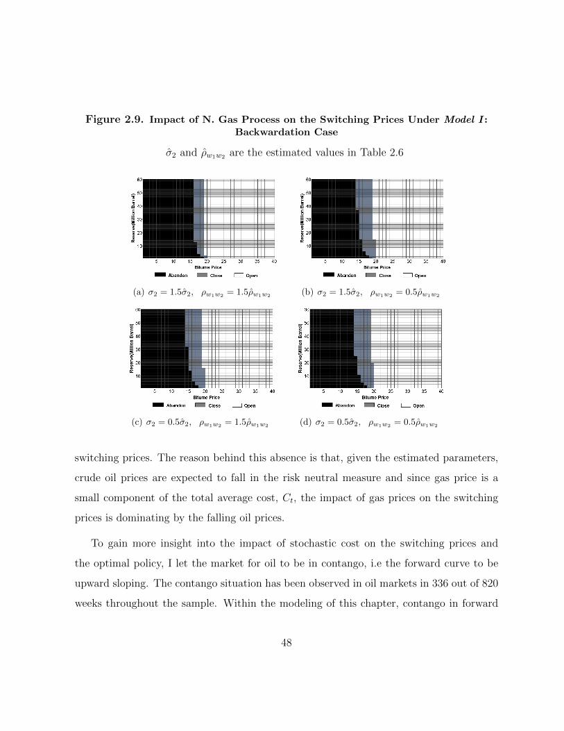
Figure 2.9. Impact of N. Gas Process on the Switching Prices Under Model I :Backwardation Case
σ2 and ρw1w2 are the estimated values in Table 2.6
(a) σ2 = 1.5σ2, ρw1w2= 1.5ρw1w2
(b) σ2 = 1.5σ2, ρw1w2= 0.5ρw1w2
(c) σ2 = 0.5σ2, ρw1w2= 1.5ρw1w2
(d) σ2 = 0.5σ2, ρw1w2= 0.5ρw1w2
switching prices. The reason behind this absence is that, given the estimated parameters,
crude oil prices are expected to fall in the risk neutral measure and since gas price is a
small component of the total average cost, Ct, the impact of gas prices on the switching
prices is dominating by the falling oil prices.
To gain more insight into the impact of stochastic cost on the switching prices and
the optimal policy, I let the market for oil to be in contango, i.e the forward curve to be
upward sloping. The contango situation has been observed in oil markets in 336 out of 820
weeks throughout the sample. Within the modeling of this chapter, contango in forward
48
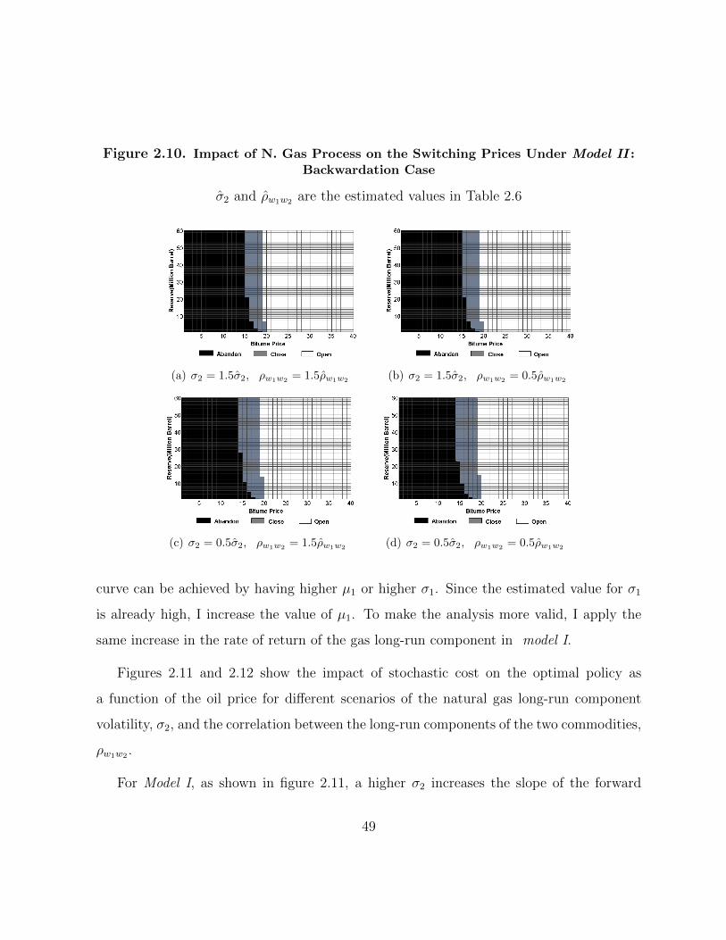
Figure 2.10. Impact of N. Gas Process on the Switching Prices Under Model II :Backwardation Case
σ2 and ρw1w2 are the estimated values in Table 2.6
(a) σ2 = 1.5σ2, ρw1w2= 1.5ρw1w2
(b) σ2 = 1.5σ2, ρw1w2= 0.5ρw1w2
(c) σ2 = 0.5σ2, ρw1w2= 1.5ρw1w2
(d) σ2 = 0.5σ2, ρw1w2= 0.5ρw1w2
curve can be achieved by having higher µ1 or higher σ1. Since the estimated value for σ1
is already high, I increase the value of µ1. To make the analysis more valid, I apply the
same increase in the rate of return of the gas long-run component in model I.
Figures 2.11 and 2.12 show the impact of stochastic cost on the optimal policy as
a function of the oil price for different scenarios of the natural gas long-run component
volatility, σ2, and the correlation between the long-run components of the two commodities,
ρw1w2 .
For Model I, as shown in figure 2.11, a higher σ2 increases the slope of the forward
49
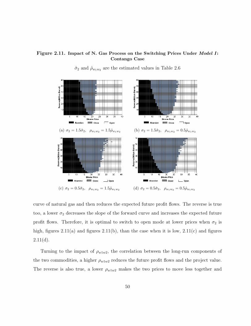
Figure 2.11. Impact of N. Gas Process on the Switching Prices Under Model I :Contango Case
σ2 and ρw1w2 are the estimated values in Table 2.6
(a) σ2 = 1.5σ2, ρw1w2= 1.5ρw1w2
(b) σ2 = 1.5σ2, ρw1w2= 0.5ρw1w2
(c) σ2 = 0.5σ2, ρw1w2= 1.5ρw1w2
(d) σ2 = 0.5σ2, ρw1w2= 0.5ρw1w2
curve of natural gas and then reduces the expected future profit flows. The reverse is true
too, a lower σ2 decreases the slope of the forward curve and increases the expected future
profit flows. Therefore, it is optimal to switch to open mode at lower prices when σ2 is
high, figures 2.11(a) and figures 2.11(b), than the case when it is low, 2.11(c) and figures
2.11(d).
Turning to the impact of ρw1w2, the correlation between the long-run components of
the two commodities, a higher ρw1w2 reduces the future profit flows and the project value.
The reverse is also true, a lower ρw1w2 makes the two prices to move less together and
50
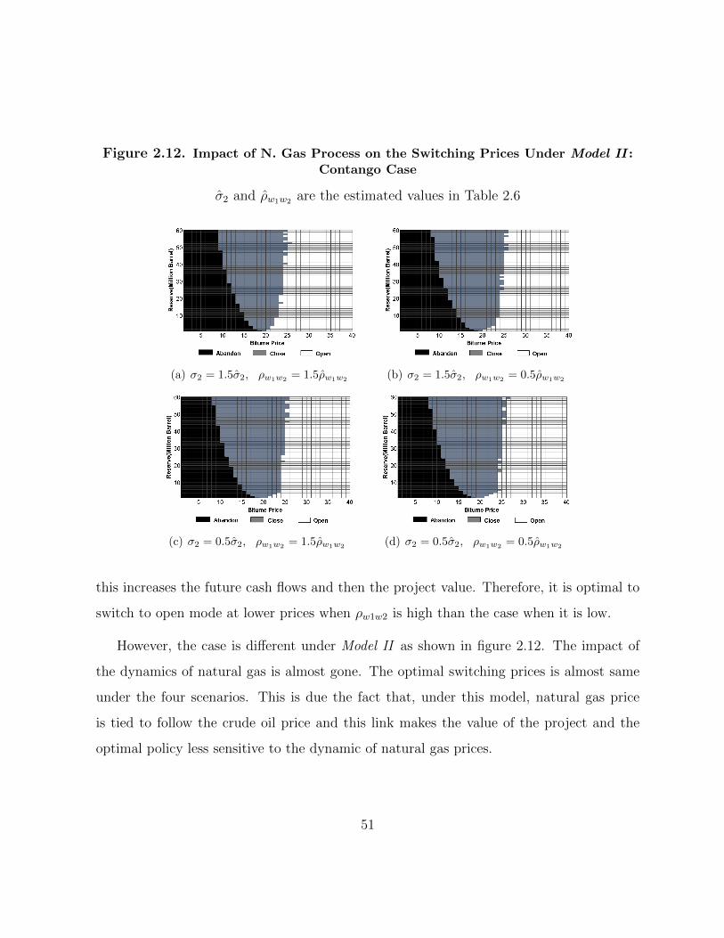
Figure 2.12. Impact of N. Gas Process on the Switching Prices Under Model II :Contango Case
σ2 and ρw1w2 are the estimated values in Table 2.6
(a) σ2 = 1.5σ2, ρw1w2= 1.5ρw1w2
(b) σ2 = 1.5σ2, ρw1w2= 0.5ρw1w2
(c) σ2 = 0.5σ2, ρw1w2= 1.5ρw1w2
(d) σ2 = 0.5σ2, ρw1w2= 0.5ρw1w2
this increases the future cash flows and then the project value. Therefore, it is optimal to
switch to open mode at lower prices when ρw1w2 is high than the case when it is low.
However, the case is different under Model II as shown in figure 2.12. The impact of
the dynamics of natural gas is almost gone. The optimal switching prices is almost same
under the four scenarios. This is due the fact that, under this model, natural gas price
is tied to follow the crude oil price and this link makes the value of the project and the
optimal policy less sensitive to the dynamic of natural gas prices.
51

2.8 Concluding Remarks
In this chapter, I study the impact of having a stochastic and a volatile component in the
extraction cost on project valuation in the oil sand industry where a substantial amount
of natural gas is used to produce oil. I show that a higher natural gas price volatility
reduces the value of the project. The chapter also shows that not only the dynamics of oil
and natural gas prices are important, but the co-movement of the two prices are also an
important factor to take in consideration in valuation and optimal operation. While the
economic links between the two markets, i.e being substitutes as sources of energy, suggests
the existence of a long-run relationship between the two prices, the chapter shows that the
empirical evidence is weak especially if one incorporates the recent divergence in the two
price series. The valuation results show that incorporating a long-run relationship between
the two markets is a very crucial decision in valuing an oil sands project and in determining
its optimal operation. The chapter shows that ignoring this long-run relationship makes
the optimal policy sensitive to the dynamic of natural gas prices. On the other hand,
incorporating this long-run relationship makes the dynamic of natural gas price process
have a vary low impact on valuation and the optimal operating policy.
52
Chapter 3
The Relationship Between Volatility
and the Forward Curve in Crude Oil
Markets
3.1 Introduction
Forward and futures contracts are fundamental tools for pricing and risk management
in energy markets, as they are in most commodities and financial markets. A forward
contract is an agreement between two parties to buy or sell an asset at a certain future
time for a set price agreed on today. A futures contract has the same general features as
a forward contract but is an exchange-traded contract, with certain standardized features.
Understanding the dynamics of the relation between spot and futures (or forward) prices
is crucial for a sound risk management analysis. For example, futures prices are usually
used as an indication of which direction the spot prices will take in the future, and the
53
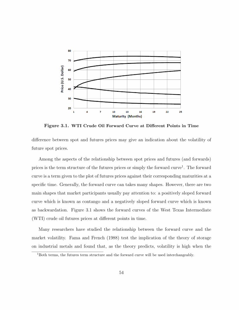
Figure 3.1. WTI Crude Oil Forward Curve at Different Points in Time
difference between spot and futures prices may give an indication about the volatility of
future spot prices.
Among the aspects of the relationship between spot prices and futures (and forwards)
prices is the term structure of the futures prices or simply the forward curve1. The forward
curve is a term given to the plot of futures prices against their corresponding maturities at a
specific time. Generally, the forward curve can takes many shapes. However, there are two
main shapes that market participants usually pay attention to: a positively sloped forward
curve which is known as contango and a negatively sloped forward curve which is known
as backwardation. Figure 3.1 shows the forward curves of the West Texas Intermediate
(WTI) crude oil futures prices at different points in time.
Many researchers have studied the relationship between the forward curve and the
market volatility. Fama and French (1988) test the implication of the theory of storage
on industrial metals and found that, as the theory predicts, volatility is high when the
1Both terms, the futures term structure and the forward curve will be used interchangeably.
54
slope of the curve is negative. Ng and Pirrong (1994) also found similar results for the
daily prices of the industrial metals during the period from September 1986 to September
1992. Litzenberger and Rabinowitz (1995) found that, in the crude oil market, volatility
is positively associated with the level of backwardation. On the other hand, Carlson et al.
(2007) and Kogan et al. (2009) found that the relation between the slope of the forward
curve and volatility is non-monotonic and has a V-shape. That is, the higher the volatility,
the steeper the slope of the curve is regardless of whether it is positive or negative.
This chapter contributes to this strand of literature by investigating empirically the
relationship between the slope of the forward curve and expected variances of the spot and
futures prices and the covariance between them in the crude oil market using another mea-
sure of the slope extracted using principal component analysis (PCA). When the relation
between the forward curve slope and volatility is studied in the literature, the commonly
used measure of the slope is the spread between the spot and futures prices. However,
there is no consensus in the literature as to what maturity date to use in calculating the
spread series. For example, Ng and Pirrong (1994) and Carlson et al. (2007) used the
spread of the third month futures price and the spot; Lien and Yang (2008) used the
second month futures contract; and, Kogan et al. (2009) used spread between the sixth
month and the third month futures prices. Borovkova (2006) shows that PCA can be used
to find a very reasonable measure of the slope of the forward curve. PCA has been used
in commodity future pricing to uncover the factors behind the movement of the forward
curve (see for example Cortazar and Schwartz (1994)). A forward curve of practically any
shape can be constructed by combining three simple shapes: the so-called level, slope and
curvature. Mathematically, these three basic shapes correspond to the first three principal
components of the array of the futures prices time series for all maturities.
Moreover, this chapter studies whether the relationship between the forward curve and
55
volatility can be used to improve the hedging performance using futures contracts. Few
researchers take account for the slope of forward curve in calculating the optimal hedge
ratio. In metal prices, Ng and Pirrong (1994) estimated a bivariate GARCH when the
slope of the forward curve, measured by the interest rate adjusted spread between spot
and futures prices, is included as a regressor in their variance and covariance equations.
They showed that the optimal hedging ratio is a function of the slope of the forward curve.
However, they have not conducted any systematic performance analysis on their results.
Recently, Lien and Yang (2008) estimated a similar model for a wide range of commodities,
including crude oil, but allowed for the asymmetric effect of the slope on variances and
covariances. They found that the in-sample and out-of-sample results both reveal that
incorporating the asymmetry effect of the slope asymmetrically into the estimated volatility
leads to better hedging in terms of risk reduction.
This chapter is organized as follows: section 3.2 is devoted to a review of the theoretical
work on the forward curve and the implications of various theories of the relation between
the slope of the forward curve and the market volatility. Section 3.3 shows how the slope
measure is constructed using PCA. The following section is for specifying the model used
to estimate the relation between volatilities and the forward curve slope. Data descrip-
tion, estimation methodology and the estimation results are shown is Sections 3.5 to 3.7.
Application to minimum variance hedge ratio is shown in section 3.8. The last section is
devoted to concluding remarks.
3.2 Theoretical Background
Many theories have been proposed to unveil the factors that govern the equilibrium rela-
tionship between spot and futures (or forward) prices and to explain the shape of forward
56
curve. The following section is a review of the most popular theories: theory of storage,
insurance perspective and hedging pressure theory, real option theory and exhaustible re-
sources theories. Each theory is explained and the implication of the theory on the shape
of forward curve is highlighted. Note that the terms forward and futures are used inter-
changeably here since the theories apply to both of them, although they are not the same
in terms of pricing if the interest rate is assumed to be stochastic.
The theory of storage has two versions: the first one relies on the notion of conve-
nience yield and was developed by Working (1949), Telser (1958) and Brennan (1958). This
version adjusts the known free-arbitrage relationship between the spot price and forward
price to account for a "convenience" yield received by the commodity inventory holders.
Commodity inventory holders (whether they are producers, consumers or speculators) re-
ceive an implicit stream of benefits when they hold inventories of the commodity. This
stream of benefits comes from the fact that they can respond flexibly and efficiently to sup-
ply and demand shocks. The theory posits that the marginal value of this yield declines
as the total level of accumulated inventory increases. That is, the benefit of inventory
holding is high when the total level of inventory in the economy is low. Consequently, the
arbitrage relation between spot and forward prices should be adjusted to account for this
yield. If Ft(τ) is the forward price at time t for delivery in τ periods, St is the spot price
of the commodity at time t, wt is the cost rate of storing the commodity as a percentage
of the spot price, rt is the interest rate for one period and It is the accumulated level of
inventory at time t, then the arbitrage relation between spot and forward is given by:
Ft(τ) = Ste(rt+wt−ct(It))τ , (3.1)
where ct is the marginal convenience yield for holding one unit of the commodity in storage
57

and ct(It) is a decreasing function of It. Thus, when the accumulated inventory level is high,
convenience yield becomes less than the interest rate plus the storage costs. In such cases,
the forward price goes higher than the spot price and contango, an upward sloping curve,
is observed. On the other hand, when the accumulated inventory level is low, convenience
yield is greater than the interest rate plus the storage costs causing the forwards price to
be lower than the spot price and backwardation, a downward sloping curve, is observed.
The second version of the theory of storage is due to Williams and Wright (1991) and
Deaton and Laroque (1996) among others. Routledge et al. (2002) extends the theory to
study the implied forward curve equilibrium. The theory relies on the fact that aggregate
inventory levels can not be reduced to be less than zero which limits the trading ability
of inventory holders. If Qt is the amount that risk neutral inventory holders, according to
their expectation of the future prices, hold in storage to be available at time t + τ , then
equilibrium price and inventory holding must satisfy:
Et(St+τ ) = Ste(rt+wt)τ if Qt > 0 (3.2a)
Et(St+τ ) ≤ Ste(rt+wt)τ if Qt = 0. (3.2b)
Equations (3.2a) and (3.2b) must hold in the equilibrium because of the optimal trading
of risk neutral inventory holders. That is, if the expected price is greater than the current
price adjusted for interest rate and storage costs, inventory holders would add to their
inventories, driving the current price up until equality is reached. On the other hand, if
the expected price is less than current price adjusted for interest rate and storage costs,
inventory holders would sell from their inventories, driving spot price down until equality
is reached or inventory is stocked out.
Under risk neutrality, the forward price is equal to the expected future spot price.
58
Therefore
Ft(τ) = Ste(rt+wt)τ if Qt > 0 (3.3a)
Ft(τ) ≤ Ste(rt+wt)τ if Qt = 0. (3.3b)
Thus, from the above equations, contango is observed in the market if aggregate inven-
tory is positive and backwardation may be observed if aggregate inventory is reduced to
zero.
In both versions of the theory, the slope of forward curve is a function of the inventory
level. A higher level of inventory is associated with the curve being in upward sloping
(contango) and a lower level of inventory is associated with the curve being in downward
sloping (backwardation). Since the volatility of the commodity price is supposed to be
a non-increasing function of the level of inventory, the theory also predicts a negative
relationship between volatility and the slope of the curve (see Ng and Pirrong (1994)).
The theory of insurance perspective is due to Keynes (see Fama and French (1987),
Bodie and Rosansky (1980), Kolb (1992) and Lautier (2005)). In this theory, producers of a
commodity would hedge against the uncertainty in the spot prices in the future by entering
into a forward contract to sell the commodity at a specified date and price. Speculators,
on the other end of the contract, take the price risk and ask for a premium by setting the
forward price less than the expected future spot price to compensate for the risk they bear.
In other words, the theory predicts that
Ft(τ) = Et(St+τ )−mt(τ) (3.4)
where mt(τ) is the risk premium due to accepting the risk of price fluctuation from t up
59

to t+ τ . Rearranging terms in equation (3.4), one gets:
Ft(τ)− St = Et(St+τ − St)−mt(τ). (3.5)
If the market is efficient, i.e. the information about expected spot prices is (or at least
mostly) reflected in the current spot price, the risk premium would dominate the difference
between forward price and current spot price. Since the risk premium is higher for bearing
the price risk for a longer time, i.e. mt(τ) is an increasing function of τ , the market finds
itself in backwardation.
Hedging pressure theory can be seen as a continuation of the insurance perspective
theory (see Change (1985), Bessembinder (1992), Roon et al. (2000), Dinceler et al. (2003)
and Gorton et al. (2007)). The assumption under the insurance perspective theory is that
producers of the commodity dominate the hedging positions in forward or futures markets.
In hedging pressure theory, the reverse might happen. In some markets, consumers of the
commodity dominate the hedging positions of forward contracts. In this case, to induce
risk-averse speculators, hedgers would offer a higher price than what is expected in the
future. Thus, the risk premium, mt(τ), would be negative and, under market efficiency,
contango is observed in the market. In summary, the theory predicts that the net position
of hedgers (the hedging pressure) determines the sign of the risk premium mt(τ) and, in
turn, the slope of the forward curve. Moreover, since higher volatility implies higher risk
premium, the theory also predicts that a steeper slope is associated with higher volatility
whether in backwardation or contango.
The third theory is the real option theory proposed by Litzenberger and Rabinowitz
(1995). The authors distinguish between strong backwardation when futures prices are
lower than the spot ones, i.e. Ft(τ) < St, and weak backwardation when discounted
60
futures prices are lower than the spot ones, i.e. Ft(τ)e−rτ < St. They observed that
between February 1984 and April 1992 around 90 percent of the time the oil forward curve
was in weak backwardation and around 77 percent of time it was in strong backwardation.
Accordingly, they proposed a theory of backwardation to resolve this empirical observation.
They assume that oil reserves are owned by a continuum of price taking oil producers
with heterogeneous extraction costs that rise at the rate of interest. Each oil reserve is
characterized as a call option where the owner has the option to produce now and pay the
cost of extraction (and get the payoff of price minus the extraction cost) or wait to produce
in the next period (keep the option alive). Denote xi as the marginal extraction cost at
time t + 1 for producer i and C(k) as a call option where k is the strike price. Moreover,
assume that extraction cost rises at the rate of interest (i.e xit = xie−r) then, the optimal
rule for each producer is:
Produce at time t if St − xie−r > Ct(xi)
Produce at time t+ 1 if St − xie−r < Ct(xi)
Indifferent if St − xie−r = Ct(xi).
The authors showed that there is one extraction cost, xm, such that producers for whom
their extraction costs are above this value will defer production to the next period and
producers for whom their extraction costs are below this value will produce in the current
period. Thus, part of the oil reserves will be produced at time t and part will be delayed
for future production. In the equilibrium St − xme−r = Ct(xm) should hold. Combining
this equation with the put and call parity, Ct(xm) = Pt(x
m) + e−r(Ft,t+1 − xm), one gets
Degree of Weak Backwardation = St − e−rFt,t+1 = Pt(xm). (3.6)
That is, the degree of weak backwardation is equal to the value of a put option with an
61

exercise price equal to the extraction cost of the marginal producer. Equation (3.6) implies
that in order to have non-zero production, the market should be in weak backwardation,
i.e. St − e−rFt,t+1 is strictly positive. If it is zero then the option value will be zero,
which means that the extraction cost of the marginal producer, xm, is so high that no
production will take place. Thus, the theory predicts that the market should be all the
time in weak backwardation and that weak backwardation is necessary for production.
Strong backwardation is observed when volatility is high. The intuition for the theory
is that when the market is volatile, the value of delaying production increases, causing
current prices to increase relative to futures prices. However, this theory has been brought
to question when recent data showed that being in contango is actually quite frequent.
Specifically, from the beginning of 1996 to the end 2008, the market was in contango 40
percent of the time.
The fourth theory is due to Hotelling (1931). He postulated a theory of the price
movement of an exhaustible resource. The theory shows that if competitive risk-neutral
producers with zero marginal extraction costs can make costless supply adjustments, then
the spot price should rise at the risk-free interest rate. Since under risk neutrality, the
expected future spot price is equivalent to the forward price, the theory predicts that
forward prices should be higher than the spot ones by the risk free rate. In other words, the
slope of the forward curve is always positive and equal to the risk-free rate. The predictions
of the earlier literature based on Hotelling’s theory are clearly inconsistent with the data
since, in reality, forward curves can be either in backwardation or in contango. Many
researchers extend the basic model and introduce some features of resource markets that
would cause the price predicted by theory to have better reconciliation with the observed
data (see Gaudet (2007) and Slade and Thille (2009) for reviews). However, the main
result of this literature is that exhaustibility of a commodity leads to a rising prices at
62
least in the long-run.
In the fifth theory, Carlson et al. (2007) proposed an equilibrium model for ex-
haustible resources, such as crude oil, where supply adjustment is not costless. In their
model, increasing the supply above historical average is costly but not decreasing it. Thus,
a supply adjustment to a positive demand shock is limited and backwardation may be
observed. When there is an adverse demand shock, since decreasing supply is not costly,
supply adjusts accordingly and exhaustibility causes the market to be in contango, as in
Hotelling-based models. Therefore, whether the market is in backwardation or contango
depends on whether the demand shock is positive or negative and whether production is
below its historical average or not. Moreover, the theory predicts that a high level of both
backwardation and contango is associated with a high level of demand shocks and, in turn,
high level of volatility in the price change.
Table 3.1 summarizes the implications of each of the above theories on shape of the
forward curve.
3.3 PCA Slope Measure
Principal component analysis (PCA) is a statistical technique that deals with a large
number of (correlated) variables and reduces them to a smaller number of uncorrelated
linear combinations, called principal components, that account for the most variability in
the original variables. More details about PCA can be found in Jolliffe (2002).
Applying PCA to crude oil futures returns, Figure (3.2) shows the loadings of the
first and the second principal components of the crude oil futures returns which together
account for about 99% of the variation in all futures returns. It is clear from the figure that
63
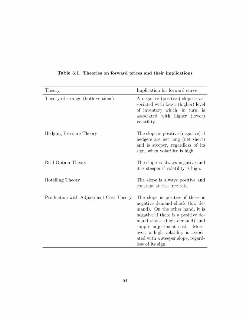
Table 3.1. Theories on forward prices and their implications
Theory Implication for forward curve
Theory of storage (both versions) A negative (positive) slope is as-sociated with lower (higher) levelof inventory which, in turn, isassociated with higher (lower)volatility.
Hedging Pressure Theory The slope is positive (negative) ifhedgers are net long (net short)and is steeper, regardless of itssign, when volatility is high.
Real Option Theory The slope is always negative andit is steeper if volatility is high.
Hotelling Theory The slope is always positive andconstant at risk free rate.
Production with Adjustment Cost Theory The slope is positive if there isnegative demand shock (low de-mand). On the other hand, it isnegative if there is a positive de-mand shock (high demand) andsupply adjustment cost. More-over, a high volatility is associ-ated with a steeper slope, regard-less of its sign.
64
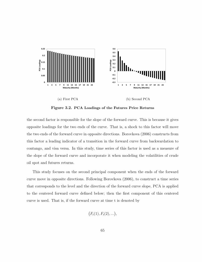
0
0.05
0.1
0.15
0.2
0.25
1 3 5 7 9 11 13 15 17 19 21 23
PC
A L
oad
ings
Maturity (Months)
(a) First PCA
-0.3
-0.2
-0.1
0
0.1
0.2
0.3
0.4
0.5
0.6
1 3 5 7 9 11 13 15 17 19 21 23
PC
A L
oad
ings
Maturity (Months)
(b) Second PCA
Figure 3.2. PCA Loadings of the Futures Price Returns
the second factor is responsible for the slope of the forward curve. This is because it gives
opposite loadings for the two ends of the curve. That is, a shock to this factor will move
the two ends of the forward curve in opposite directions. Borovkova (2006) constructs from
this factor a leading indicator of a transition in the forward curve from backwardation to
contango, and visa versa. In this study, time series of this factor is used as a measure of
the slope of the forward curve and incorporate it when modeling the volatilities of crude
oil spot and futures returns.
This study focuses on the second principal component when the ends of the forward
curve move in opposite directions. Following Borovkova (2006), to construct a time series
that corresponds to the level and the direction of the forward curve slope, PCA is applied
to the centered forward curve defined below; then the first component of this centered
curve is used. That is, if the forward curve at time t is denoted by
(Ft(1), Ft(2), ...
),
65
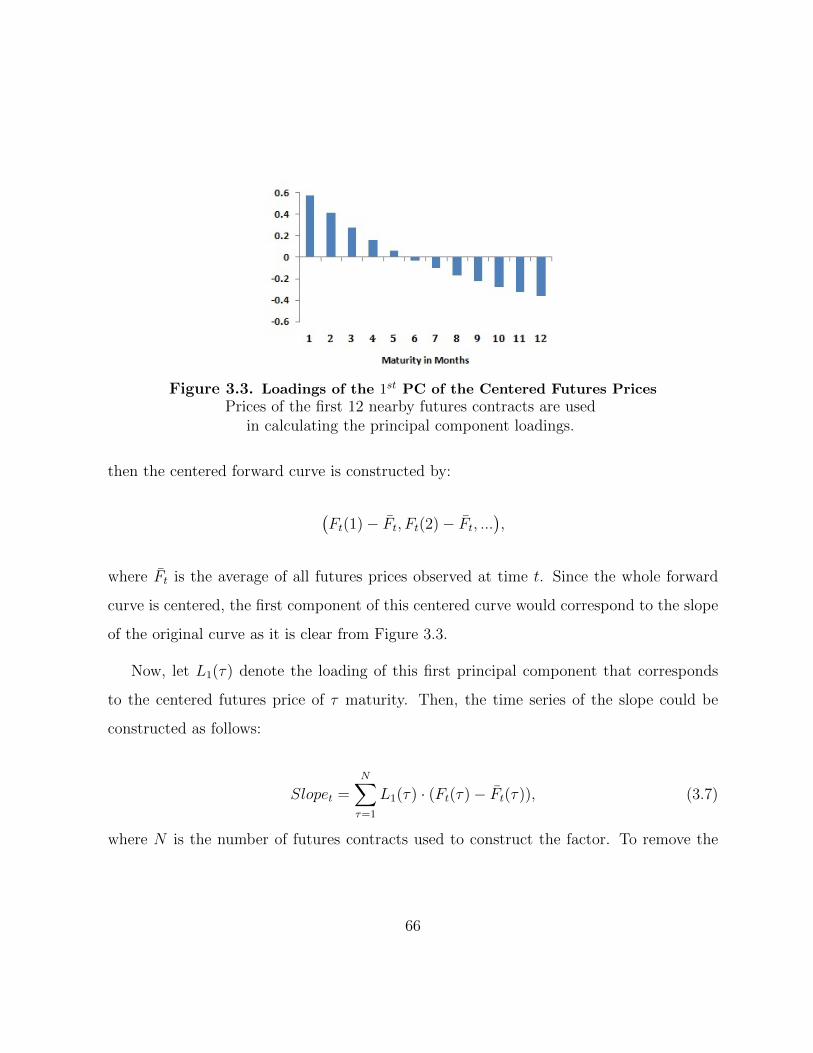
Figure 3.3. Loadings of the 1st PC of the Centered Futures PricesPrices of the first 12 nearby futures contracts are used
in calculating the principal component loadings.
then the centered forward curve is constructed by:
(Ft(1)− Ft, Ft(2)− Ft, ...
),
where Ft is the average of all futures prices observed at time t. Since the whole forward
curve is centered, the first component of this centered curve would correspond to the slope
of the original curve as it is clear from Figure 3.3.
Now, let L1(τ) denote the loading of this first principal component that corresponds
to the centered futures price of τ maturity. Then, the time series of the slope could be
constructed as follows:
Slopet =N∑τ=1
L1(τ) · (Ft(τ)− Ft(τ)), (3.7)
where N is the number of futures contracts used to construct the factor. To remove the
66
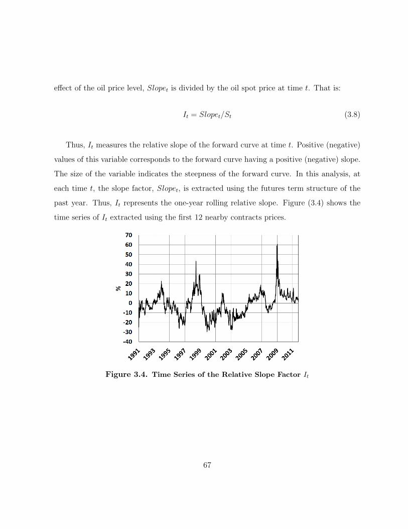
effect of the oil price level, Slopet is divided by the oil spot price at time t. That is:
It = Slopet/St (3.8)
Thus, It measures the relative slope of the forward curve at time t. Positive (negative)
values of this variable corresponds to the forward curve having a positive (negative) slope.
The size of the variable indicates the steepness of the forward curve. In this analysis, at
each time t, the slope factor, Slopet, is extracted using the futures term structure of the
past year. Thus, It represents the one-year rolling relative slope. Figure (3.4) shows the
time series of It extracted using the first 12 nearby contracts prices.
Figure 3.4. Time Series of the Relative Slope Factor It
67
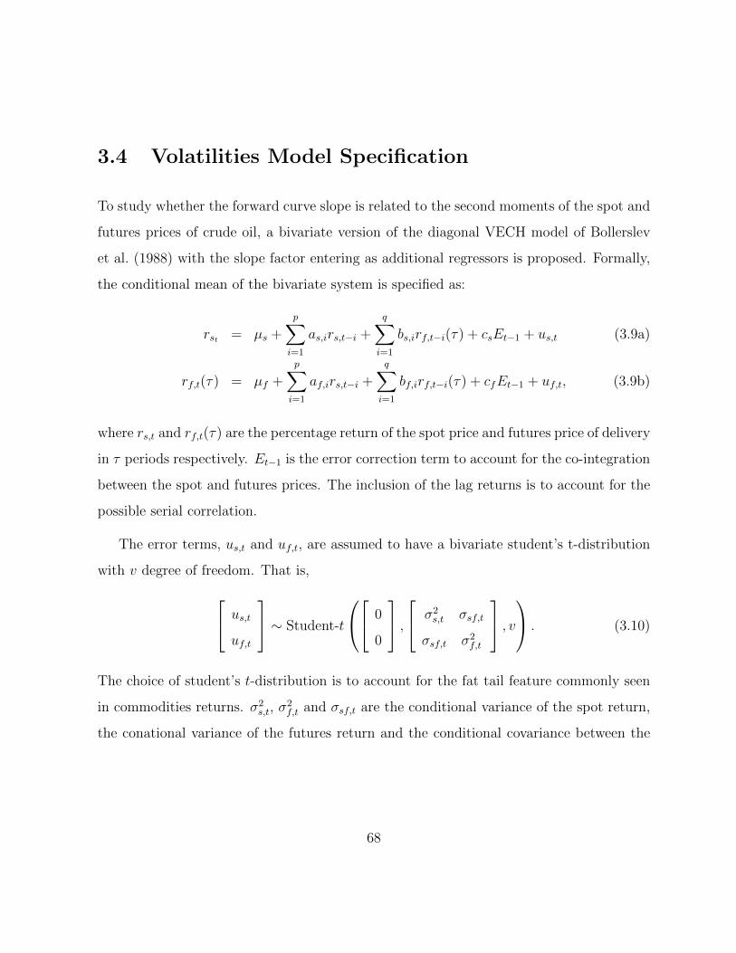
3.4 Volatilities Model Specification
To study whether the forward curve slope is related to the second moments of the spot and
futures prices of crude oil, a bivariate version of the diagonal VECH model of Bollerslev
et al. (1988) with the slope factor entering as additional regressors is proposed. Formally,
the conditional mean of the bivariate system is specified as:
rst = µs +
p∑i=1
as,irs,t−i +
q∑i=1
bs,irf,t−i(τ) + csEt−1 + us,t (3.9a)
rf,t(τ) = µf +
p∑i=1
af,irs,t−i +
q∑i=1
bf,irf,t−i(τ) + cfEt−1 + uf,t, (3.9b)
where rs,t and rf,t(τ) are the percentage return of the spot price and futures price of delivery
in τ periods respectively. Et−1 is the error correction term to account for the co-integration
between the spot and futures prices. The inclusion of the lag returns is to account for the
possible serial correlation.
The error terms, us,t and uf,t, are assumed to have a bivariate student’s t-distribution
with v degree of freedom. That is, us,t
uf,t
∼ Student-t
0
0
, σ2
s,t σsf,t
σsf,t σ2f,t
, v . (3.10)
The choice of student’s t-distribution is to account for the fat tail feature commonly seen
in commodities returns. σ2s,t, σ
2f,t and σsf,t are the conditional variance of the spot return,
the conational variance of the futures return and the conditional covariance between the
68
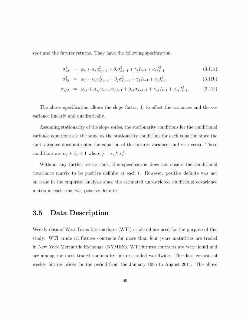
spot and the futures returns. They have the following specification:
σ2s,t = ωs + αsu
2s,t−1 + βsσ
2s,t−1 + γsIt−1 + κsI
2t−1 (3.11a)
σ2f,t = ωf + αfu
2f,t−1 + βfσ
2f,t−1 + γfIt−1 + κfI
2t−1 (3.11b)
σsf,t = ωsf + αsfus,t−1uf,t−1 + βsfσfs,t−1 + γsfIt−1 + κsfI2t−1. (3.11c)
The above specification allows the slope factor, It to affect the variances and the co-
variance linearly and quadratically.
Assuming stationarity of the slope series, the stationarity conditions for the conditional
variance equations are the same as the stationarity conditions for each equation since the
spot variance does not enter the equation of the futures variance, and visa versa. These
conditions are αj + βj < 1 where j = s, f, sf .
Without any further restrictions, this specification does not ensure the conditional
covariance matrix to be positive definite at each t. However, positive definite was not
an issue in the empirical analysis since the estimated unrestricted conditional covariance
matrix at each time was positive definite.
3.5 Data Description
Weekly data of West Texas Intermediate (WTI) crude oil are used for the purpose of this
study. WTI crude oil futures contracts for more than four years maturities are traded
in New York Mercantile Exchange (NYMEX). WTI futures contracts are very liquid and
are among the most traded commodity futures traded worldwide. The data consists of
weekly futures prices for the period from the January 1995 to August 2011. The above
69
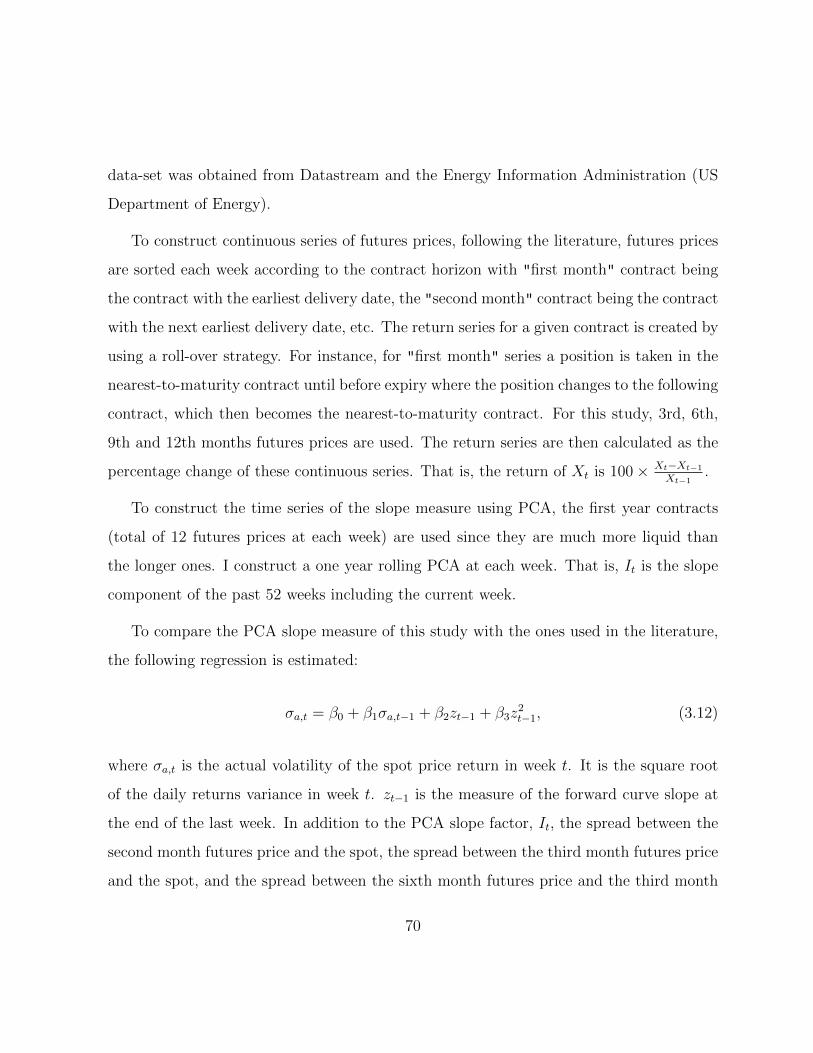
data-set was obtained from Datastream and the Energy Information Administration (US
Department of Energy).
To construct continuous series of futures prices, following the literature, futures prices
are sorted each week according to the contract horizon with "first month" contract being
the contract with the earliest delivery date, the "second month" contract being the contract
with the next earliest delivery date, etc. The return series for a given contract is created by
using a roll-over strategy. For instance, for "first month" series a position is taken in the
nearest-to-maturity contract until before expiry where the position changes to the following
contract, which then becomes the nearest-to-maturity contract. For this study, 3rd, 6th,
9th and 12th months futures prices are used. The return series are then calculated as the
percentage change of these continuous series. That is, the return of Xt is 100× Xt−Xt−1
Xt−1.
To construct the time series of the slope measure using PCA, the first year contracts
(total of 12 futures prices at each week) are used since they are much more liquid than
the longer ones. I construct a one year rolling PCA at each week. That is, It is the slope
component of the past 52 weeks including the current week.
To compare the PCA slope measure of this study with the ones used in the literature,
the following regression is estimated:
σa,t = β0 + β1σa,t−1 + β2zt−1 + β3z2t−1, (3.12)
where σa,t is the actual volatility of the spot price return in week t. It is the square root
of the daily returns variance in week t. zt−1 is the measure of the forward curve slope at
the end of the last week. In addition to the PCA slope factor, It, the spread between the
second month futures price and the spot, the spread between the third month futures price
and the spot, and the spread between the sixth month futures price and the third month
70
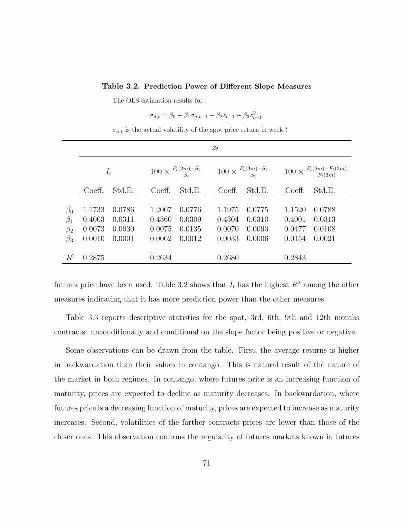
Table 3.2. Prediction Power of Different Slope Measures
The OLS estimation results for :
σa,t = β0 + β1σa,t−1 + β2zt−1 + β3z2t−1,
σa,t is the actual volatility of the spot price return in week t
zt
It 100× Ft(2m)−St
St100× Ft(3m)−St
St100× Ft(6m)−Ft(3m)
Ft(3m)
Coeff. Std.E. Coeff. Std.E. Coeff. Std.E. Coeff. Std.E.
β0 1.1733 0.0786 1.2007 0.0776 1.1975 0.0775 1.1520 0.0788β1 0.4003 0.0311 0.4360 0.0309 0.4304 0.0310 0.4001 0.0313β2 0.0073 0.0030 0.0075 0.0135 0.0070 0.0090 0.0477 0.0108β3 0.0010 0.0001 0.0062 0.0012 0.0033 0.0006 0.0154 0.0021
R2 0.2875 0.2634 0.2680 0.2843
futures price have been used. Table 3.2 shows that It has the highest R2 among the other
measures indicating that it has more prediction power than the other measures.
Table 3.3 reports descriptive statistics for the spot, 3rd, 6th, 9th and 12th months
contracts: unconditionally and conditional on the slope factor being positive or negative.
Some observations can be drawn from the table. First, the average returns is higher
in backwardation than their values in contango. This is natural result of the nature of
the market in both regimes. In contango, where futures price is an increasing function of
maturity, prices are expected to decline as maturity decreases. In backwardation, where
futures price is a decreasing function of maturity, prices are expected to increase as maturity
increases. Second, volatilities of the farther contracts prices are lower than those of the
closer ones. This observation confirms the regularity of futures markets known in futures
71
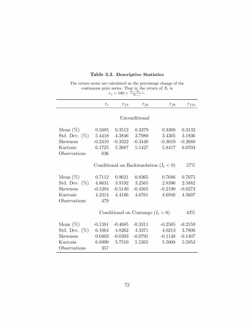
Table 3.3. Descriptive Statistics
The return series are calculated as the percentage change of thecontinuous price series. That is, the return of Xt is
rx = 100× Xt−Xt−1
Xt−1.
rs rf3 rf6 rf9 rf12
Unconditional
Mean (%) 0.3485 0.3512 0.3379 0.3300 0.3132Std. Dev. (%) 5.4418 4.3846 3.7980 3.4305 3.1836Skewness -0.2410 -0.3322 -0.3440 -0.3019 -0.2688Kurtosis 6.1725 5.2687 5.5427 5.8417 6.0703Observations 836
Conditional on Backwardation (It < 0) 57%
Mean (%) 0.7112 0.9621 0.8365 0.7686 0.7075Std. Dev. (%) 4.8631 3.9192 3.2565 2.8396 2.5882Skewness -0.5204 -0.5140 -0.4565 -0.2190 -0.0273Kurtosis 4.2314 4.4186 4.6761 4.6948 4.5607Observations 479
Conditional on Contango (It > 0) 43%
Mean (%) -0.1381 -0.4685 -0.3311 -0.2585 -0.2159Std. Dev. (%) 6.1064 4.8262 4.3371 4.0213 3.7800Skewness 0.0403 -0.0393 -0.0791 -0.1148 -0.1407Kurtosis 6.8990 5.7510 5.5265 5.5008 5.5953Observations 357
72
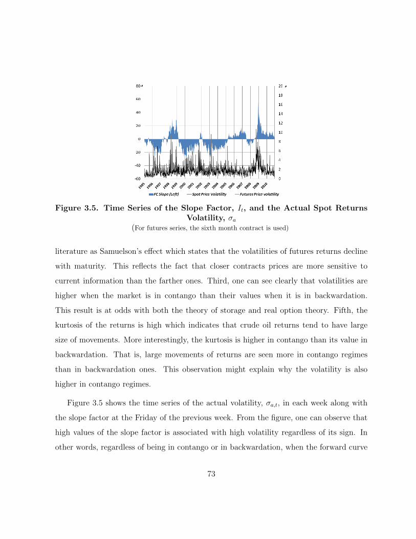
Figure 3.5. Time Series of the Slope Factor, It, and the Actual Spot ReturnsVolatility, σa
(For futures series, the sixth month contract is used)
literature as Samuelson’s effect which states that the volatilities of futures returns decline
with maturity. This reflects the fact that closer contracts prices are more sensitive to
current information than the farther ones. Third, one can see clearly that volatilities are
higher when the market is in contango than their values when it is in backwardation.
This result is at odds with both the theory of storage and real option theory. Fifth, the
kurtosis of the returns is high which indicates that crude oil returns tend to have large
size of movements. More interestingly, the kurtosis is higher in contango than its value in
backwardation. That is, large movements of returns are seen more in contango regimes
than in backwardation ones. This observation might explain why the volatility is also
higher in contango regimes.
Figure 3.5 shows the time series of the actual volatility, σa,t, in each week along with
the slope factor at the Friday of the previous week. From the figure, one can observe that
high values of the slope factor is associated with high volatility regardless of its sign. In
other words, regardless of being in contango or in backwardation, when the forward curve
73
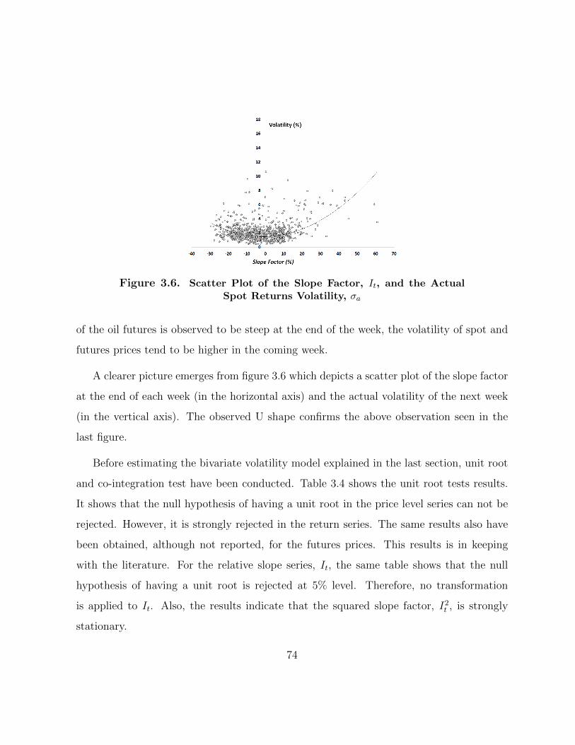
Figure 3.6. Scatter Plot of the Slope Factor, It, and the ActualSpot Returns Volatility, σa
of the oil futures is observed to be steep at the end of the week, the volatility of spot and
futures prices tend to be higher in the coming week.
A clearer picture emerges from figure 3.6 which depicts a scatter plot of the slope factor
at the end of each week (in the horizontal axis) and the actual volatility of the next week
(in the vertical axis). The observed U shape confirms the above observation seen in the
last figure.
Before estimating the bivariate volatility model explained in the last section, unit root
and co-integration test have been conducted. Table 3.4 shows the unit root tests results.
It shows that the null hypothesis of having a unit root in the price level series can not be
rejected. However, it is strongly rejected in the return series. The same results also have
been obtained, although not reported, for the futures prices. This results is in keeping
with the literature. For the relative slope series, It, the same table shows that the null
hypothesis of having a unit root is rejected at 5% level. Therefore, no transformation
is applied to It. Also, the results indicate that the squared slope factor, I2t , is strongly
stationary.
74
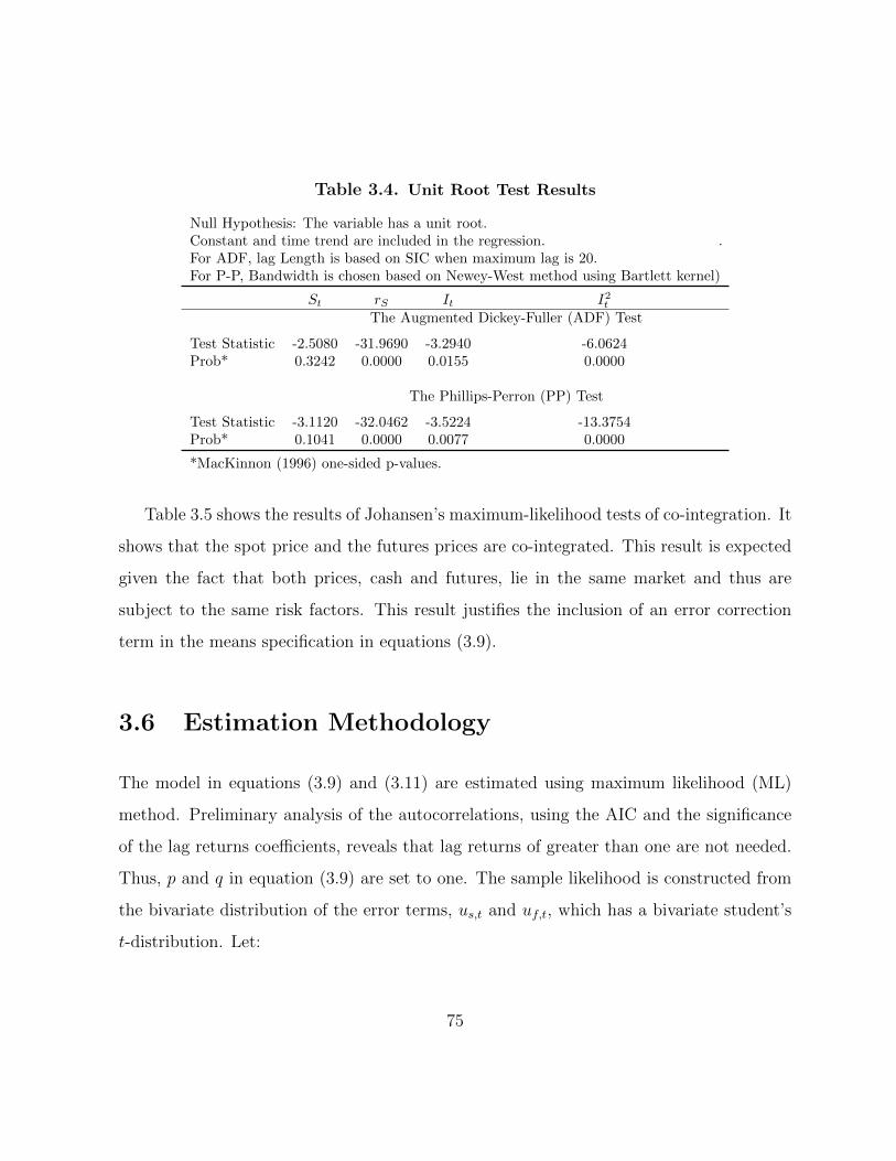
Table 3.4. Unit Root Test Results
Null Hypothesis: The variable has a unit root.Constant and time trend are included in the regression. .For ADF, lag Length is based on SIC when maximum lag is 20.For P-P, Bandwidth is chosen based on Newey-West method using Bartlett kernel)
St rS It I2tThe Augmented Dickey-Fuller (ADF) Test
Test Statistic -2.5080 -31.9690 -3.2940 -6.0624Prob* 0.3242 0.0000 0.0155 0.0000
The Phillips-Perron (PP) Test
Test Statistic -3.1120 -32.0462 -3.5224 -13.3754Prob* 0.1041 0.0000 0.0077 0.0000
*MacKinnon (1996) one-sided p-values.
Table 3.5 shows the results of Johansen’s maximum-likelihood tests of co-integration. It
shows that the spot price and the futures prices are co-integrated. This result is expected
given the fact that both prices, cash and futures, lie in the same market and thus are
subject to the same risk factors. This result justifies the inclusion of an error correction
term in the means specification in equations (3.9).
3.6 Estimation Methodology
The model in equations (3.9) and (3.11) are estimated using maximum likelihood (ML)
method. Preliminary analysis of the autocorrelations, using the AIC and the significance
of the lag returns coefficients, reveals that lag returns of greater than one are not needed.
Thus, p and q in equation (3.9) are set to one. The sample likelihood is constructed from
the bivariate distribution of the error terms, us,t and uf,t, which has a bivariate student’s
t-distribution. Let:
75
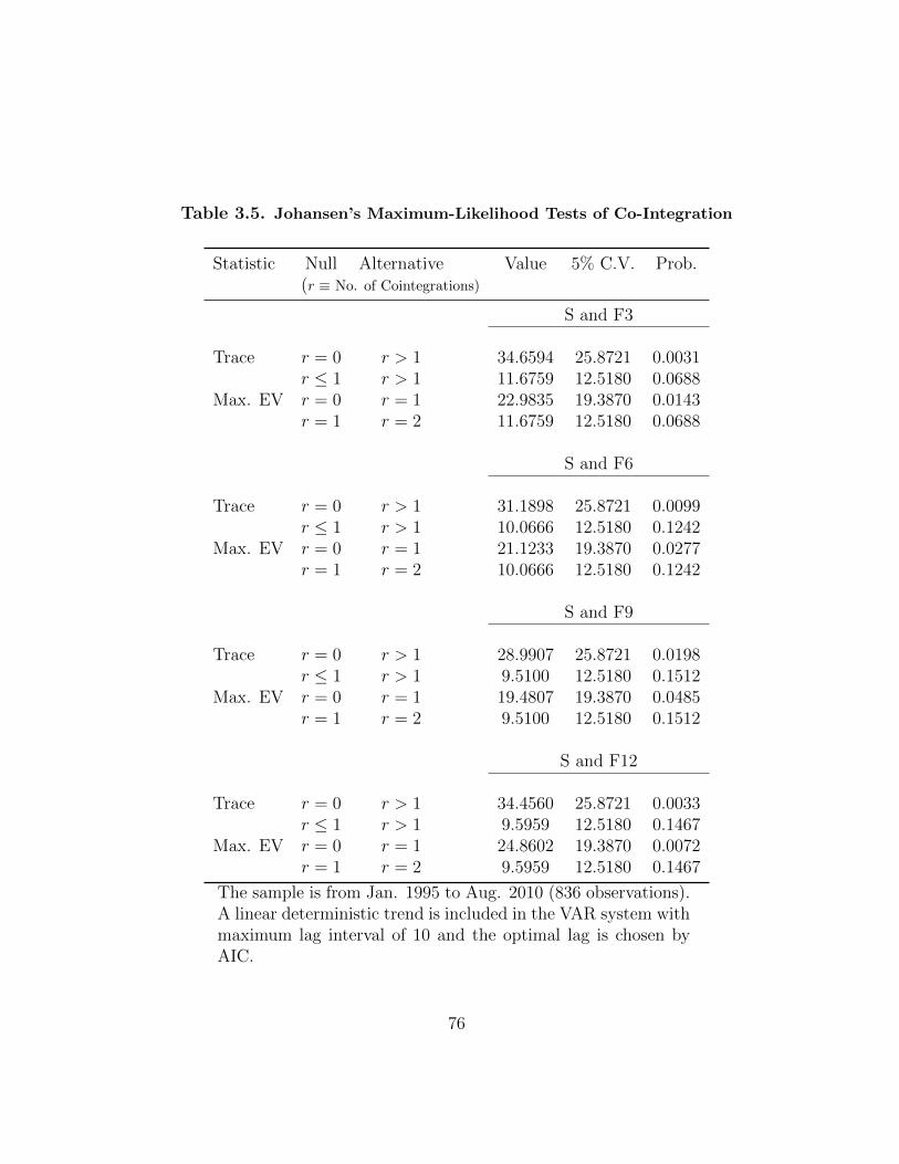
Table 3.5. Johansen’s Maximum-Likelihood Tests of Co-Integration
Statistic Null Alternative Value 5% C.V. Prob.(r ≡ No. of Cointegrations)
S and F3
Trace r = 0 r > 1 34.6594 25.8721 0.0031r ≤ 1 r > 1 11.6759 12.5180 0.0688
Max. EV r = 0 r = 1 22.9835 19.3870 0.0143r = 1 r = 2 11.6759 12.5180 0.0688
S and F6
Trace r = 0 r > 1 31.1898 25.8721 0.0099r ≤ 1 r > 1 10.0666 12.5180 0.1242
Max. EV r = 0 r = 1 21.1233 19.3870 0.0277r = 1 r = 2 10.0666 12.5180 0.1242
S and F9
Trace r = 0 r > 1 28.9907 25.8721 0.0198r ≤ 1 r > 1 9.5100 12.5180 0.1512
Max. EV r = 0 r = 1 19.4807 19.3870 0.0485r = 1 r = 2 9.5100 12.5180 0.1512
S and F12
Trace r = 0 r > 1 34.4560 25.8721 0.0033r ≤ 1 r > 1 9.5959 12.5180 0.1467
Max. EV r = 0 r = 1 24.8602 19.3870 0.0072r = 1 r = 2 9.5959 12.5180 0.1467
The sample is from Jan. 1995 to Aug. 2010 (836 observations).A linear deterministic trend is included in the VAR system withmaximum lag interval of 10 and the optimal lag is chosen byAIC.
76
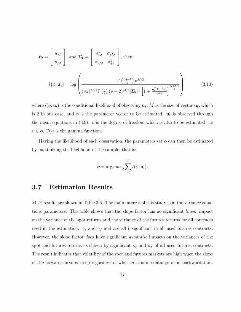
ut =
us,t
uf,t
, and Σt =
σ2s,t σsf,t
σsf,t σ2f,t
, then:
l(φ; ut
)= log
Γ(v+M
2
)vM/2
(vπ)M/2Γ(v2
)(v − 2)M/2|Σt|
12
[1 +
u>t Σ−1t ut
v−2
] (v+M)2
(3.13)
where l(φ; ut) is the conditional likelihood of observing ut, M is the size of vector ut, which
is 2 in our case, and φ is the parameter vector to be estimated. ut is observed through
the mean equations in (3.9). v is the degree of freedom which is also to be estimated, i.e
v ∈ φ. Γ(·) is the gamma function.
Having the likelihood of each observation, the parameters set φ can then be estimated
by maximizing the likelihood of the sample, that is:
φ = arg maxφ
T∑t=1
l(φ; ut).
3.7 Estimation Results
MLE results are shown in Table 3.6. The main interest of this study is in the variance equa-
tions parameters. The table shows that the slope factor has no significant linear impact
on the variance of the spot returns and the variance of the futures returns for all contracts
used in the estimation. γs and γf and are all insignificant in all used futures contracts.
However, the slope factor does have significant quadratic impacts on the variances of the
spot and futures returns as shown by significant κs and κf of all used futures contracts.
The result indicates that volatility of the spot and futures markets are high when the slope
of the forward curve is steep regardless of whether it is in contango or in backwardation.
77
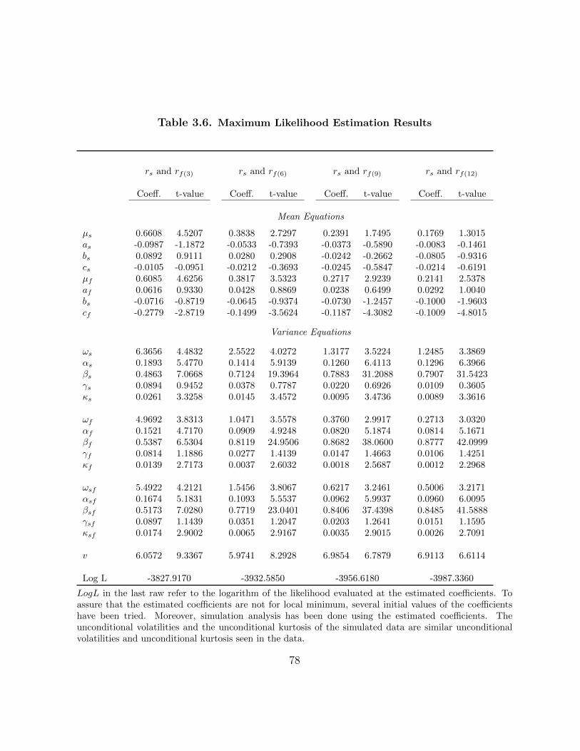
Table 3.6. Maximum Likelihood Estimation Results
rs and rf(3) rs and rf(6) rs and rf(9) rs and rf(12)
Coeff. t-value Coeff. t-value Coeff. t-value Coeff. t-value
Mean Equations
µs 0.6608 4.5207 0.3838 2.7297 0.2391 1.7495 0.1769 1.3015as -0.0987 -1.1872 -0.0533 -0.7393 -0.0373 -0.5890 -0.0083 -0.1461bs 0.0892 0.9111 0.0280 0.2908 -0.0242 -0.2662 -0.0805 -0.9316cs -0.0105 -0.0951 -0.0212 -0.3693 -0.0245 -0.5847 -0.0214 -0.6191µf 0.6085 4.6256 0.3817 3.5323 0.2717 2.9239 0.2141 2.5378af 0.0616 0.9330 0.0428 0.8869 0.0238 0.6499 0.0292 1.0040bs -0.0716 -0.8719 -0.0645 -0.9374 -0.0730 -1.2457 -0.1000 -1.9603cf -0.2779 -2.8719 -0.1499 -3.5624 -0.1187 -4.3082 -0.1009 -4.8015
Variance Equations
ωs 6.3656 4.4832 2.5522 4.0272 1.3177 3.5224 1.2485 3.3869αs 0.1893 5.4770 0.1414 5.9139 0.1260 6.4113 0.1296 6.3966βs 0.4863 7.0668 0.7124 19.3964 0.7883 31.2088 0.7907 31.5423γs 0.0894 0.9452 0.0378 0.7787 0.0220 0.6926 0.0109 0.3605κs 0.0261 3.3258 0.0145 3.4572 0.0095 3.4736 0.0089 3.3616
ωf 4.9692 3.8313 1.0471 3.5578 0.3760 2.9917 0.2713 3.0320αf 0.1521 4.7170 0.0909 4.9248 0.0820 5.1874 0.0814 5.1671βf 0.5387 6.5304 0.8119 24.9506 0.8682 38.0600 0.8777 42.0999γf 0.0814 1.1886 0.0277 1.4139 0.0147 1.4663 0.0106 1.4251κf 0.0139 2.7173 0.0037 2.6032 0.0018 2.5687 0.0012 2.2968
ωsf 5.4922 4.2121 1.5456 3.8067 0.6217 3.2461 0.5006 3.2171αsf 0.1674 5.1831 0.1093 5.5537 0.0962 5.9937 0.0960 6.0095βsf 0.5173 7.0280 0.7719 23.0401 0.8406 37.4398 0.8485 41.5888γsf 0.0897 1.1439 0.0351 1.2047 0.0203 1.2641 0.0151 1.1595κsf 0.0174 2.9002 0.0065 2.9167 0.0035 2.9015 0.0026 2.7091
v 6.0572 9.3367 5.9741 8.2928 6.9854 6.7879 6.9113 6.6114
Log L -3827.9170 -3932.5850 -3956.6180 -3987.3360
LogL in the last raw refer to the logarithm of the likelihood evaluated at the estimated coefficients. Toassure that the estimated coefficients are not for local minimum, several initial values of the coefficientshave been tried. Moreover, simulation analysis has been done using the estimated coefficients. Theunconditional volatilities and the unconditional kurtosis of the simulated data are similar unconditionalvolatilities and unconditional kurtosis seen in the data.
78
This result supports the hedging pressure theory and the adjustment cost theory and it
also in line with the empirical work of Carlson et al. (2007) and Kogan et al. (2009). The
results are at odds with the theory of storage and the real option theory as shown section
3.2.
More interestingly, the results show that not only variances are function of the steepness
of the forward curve slope, but the covariance between the spot and futures returns is also
impacted by of the steepness of the slope quadratically as evidenced by the significant κsf .
That is, the higher the slope of the forward curve the closer the spot and futures markets are
expected to be regardless whether the market is in contango or backwardation. This result
indicates that when high uncertainty is expected, both spot and futures prices respond
similarly to a shock in the market2.
To further investigate the above results, the Wald’s χ2 test is used to test the following
two null hypothesis: the first one is that the linear impact is zero, i.e γs = γsf = γf = 0
and the second one is that the quadratic impact is zero, i.e. κs = κf = κsf = 0. Table
3.7 shows the results of the Wald’s χ2 test. The test results fail to reject the first one but
strongly reject the second one.
Thus, the above results shows that the slope of forward curve has a significant power
to predict the volatility in the market. Within the framework of the model of this study,
the contribution of the slope factor to the innovations in variances and the covariance
can be calculated as shown by Ng and Pirrong (1994), who estimated a similar model for
metals prices. From the equations in (3.11), there are two kinds of shocks that contribute
2The table also shows that the persistence of the variances (which is reflected in the value of βi wherei = s, f and sf) is increasing with the maturity of the contract. On the other hand, the impact of theinnovation on the variance (which is reflected in the value of αi where i = s, f and sf) is decreasing withthe maturity. This result has to do with Samuelson’s effect where futures variances decrease with thecontract maturity. In other words, futures prices for longer maturity response less to the shocks in thecurrent market.
79
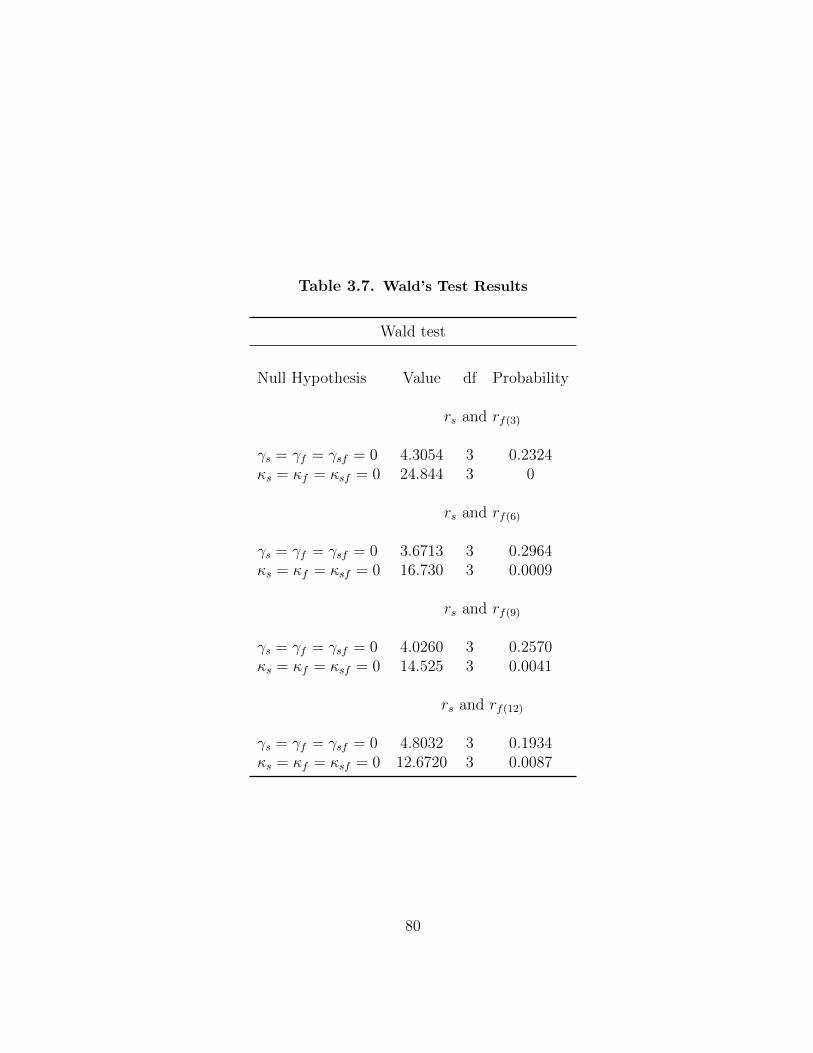
Table 3.7. Wald’s Test Results
Wald test
Null Hypothesis Value df Probability
rs and rf(3)
γs = γf = γsf = 0 4.3054 3 0.2324κs = κf = κsf = 0 24.844 3 0
rs and rf(6)
γs = γf = γsf = 0 3.6713 3 0.2964κs = κf = κsf = 0 16.730 3 0.0009
rs and rf(9)
γs = γf = γsf = 0 4.0260 3 0.2570κs = κf = κsf = 0 14.525 3 0.0041
rs and rf(12)
γs = γf = γsf = 0 4.8032 3 0.1934κs = κf = κsf = 0 12.6720 3 0.0087
80

Table 3.8. Contribution of the Forward Curve Slope on the Second Moments
The reported numbers are the averages of y(j)t =
κjI2t−1
αju2j,t−1κjI2t−1
when the
model is re-estimated with γs = γf = γsf = 0.
rs and rf3 rs and rf6 rs and rf9 rs and rf12
j = s 0.4917 0.4411 0.4004 0.3920j = f 0.427 0.3023 0.2334 0.1942j = sf 0.4470 0.3560 0.2939 0.2622
to variances and the covariance at each time: the slope of the forward curve, It, and the
squared residual returns, uj,t where j = s, f, sf . The lag of the variances and covariance
terms reflect the persistence of the effects of these two shocks. From the equations in
(3.11), the contribution of the slope factor to the total shock in the time t second moments
can be calculated as:
y(j)t =
γjIt−1 + κjI2t−1
αju2j,t−1 + γjIt−1 + κjI2
t−1
, (3.14)
where j = s, f or sf .
Since the linear impact of It is not significant, the model is re-estimated with only the
significant quadratic impact, i.e. γs = γf = γsf = 0, then y(j)t is calculated at each time
and the average values are reported in Table 3.8. The numbers show that the slope of the
forward curve explains a large fraction of the innovations in the second moments, especially
for the near months contracts.
81
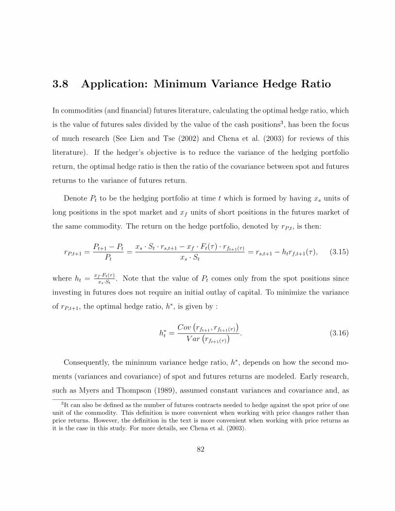
3.8 Application: Minimum Variance Hedge Ratio
In commodities (and financial) futures literature, calculating the optimal hedge ratio, which
is the value of futures sales divided by the value of the cash positions3, has been the focus
of much research (See Lien and Tse (2002) and Chena et al. (2003) for reviews of this
literature). If the hedger’s objective is to reduce the variance of the hedging portfolio
return, the optimal hedge ratio is then the ratio of the covariance between spot and futures
returns to the variance of futures return.
Denote Pt to be the hedging portfolio at time t which is formed by having xs units of
long positions in the spot market and xf units of short positions in the futures market of
the same commodity. The return on the hedge portfolio, denoted by rP,t, is then:
rP,t+1 =Pt+1 − Pt
Pt=xs · St · rs,t+1 − xf · Ft(τ) · rft+1(τ)
xs · St= rs,t+1 − htrf,t+1(τ), (3.15)
where ht =xf ·Ft(τ)
xs·St. Note that the value of Pt comes only from the spot positions since
investing in futures does not require an initial outlay of capital. To minimize the variance
of rP,t+1, the optimal hedge ratio, h∗, is given by :
h∗t =Cov
(rft+1 , rft+1(τ)
)V ar
(rft+1(τ)
) . (3.16)
Consequently, the minimum variance hedge ratio, h∗, depends on how the second mo-
ments (variances and covariance) of spot and futures returns are modeled. Early research,
such as Myers and Thompson (1989), assumed constant variances and covariance and, as
3It can also be defined as the number of futures contracts needed to hedge against the spot price of oneunit of the commodity. This definition is more convenient when working with price changes rather thanprice returns. However, the definition in the text is more convenient when working with price returns asit is the case in this study. For more details, see Chena et al. (2003).
82

a result, the optimal hedge ratio would be constant and could be easily estimated by a
least-square regression. However, the assumption of constant second moments is not real-
istic given the documented evidence that most asset prices, including commodities, have
time-varying volatilities. This implies that the optimal hedge ratio should be time varying
as well. Many researchers have recently employed various specifications to model the sec-
ond moments. For example Baillie and Myers (1991), Kroner and Sultan (1993) and Ng
and Pirrong (1994) among others used bivariate GARCH models. Lien and Wilson (2001)
suggested a stochastic volatility model. Alizadeh et al. (2008) used the Markov Regime
Switching approach.
This section studies how much improvement in hedging performance can be obtained
when the significant impact of the forward curve shape is incorporated in modeling the
second moments as seen in the last section. Again, given the insignificance of the linear
impact of the slope factor, the model in equations (3.11) are re-estimated with the linear
impacts omitted, that is γs = γf = γsf = 0. The minimum hedge ratio is then calculated
as :
h∗t =σsf,t+1
σ2f,t+1
. (3.17)
Data from January 1995 to December 2010 are used for the estimation and data from
January 2011 to October 2011 are used to evaluate the hedge performance. The 3rd
month futures contract is used in the hedging portfolio. The hedging performance is
measured by the variance of rp,t. For comparison, the hedging performance of two other
models are computed. The first one is the pure diagonal VECH which obtain by sitting
κs = κf = κsf = 0. The second one is using the OLS hedge ratio obtained by regressing
the spot returns on the furfures returns. The hedge ratios of these two models are denoted
by h(Bgarch)t and h
(OLS)t respectively. The results are shown in figure 3.7 which shows the
time series of the hedging portfolios and Table 3.9 which shows the variance of the hedging
83
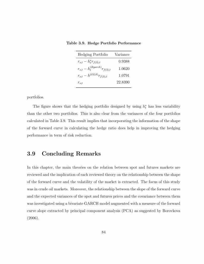
Table 3.9. Hedge Portfolio Performance
Hedging Portfolio Variance
rs,t − h∗t rf(3),t 0.9388
rs,t − h(Bgarch)t rf(3),t 1.0620
rs,t − h(OLS)rf(3),t 1.0791
rs,t 22.8390
portfolios.
The figure shows that the hedging portfolio designed by using h∗t has less variability
than the other two portfolios. This is also clear from the variances of the four portfolios
calculated in Table 3.9. This result implies that incorporating the information of the shape
of the forward curve in calculating the hedge ratio does help in improving the hedging
performance in term of risk reduction.
3.9 Concluding Remarks
In this chapter, the main theories on the relation between spot and futures markets are
reviewed and the implication of each reviewed theory on the relationship between the shape
of the forward curve and the volatility of the market is extracted. The focus of this study
was in crude oil markets. Moreover, the relationship between the slope of the forward curve
and the expected variances of the spot and futures prices and the covariance between them
was investigated using a bivariate GARCH model augmented with a measure of the forward
curve slope extracted by principal component analysis (PCA) as suggested by Borovkova
(2006).
84

Figure 3.7. Time Series of The Hedging Portfolio Return
The slope of the forward curve was found to have a significant quadratic impact on
the variances and the covariance of the spot and futures returns in the crude oil prices.
Moreover, the study shows that exploiting this relation in designing the minimum variance
hedge ratio leads to better results in term of risk reduction. A potential direction for
futures research is to study the hedging performance, when the prediction power of the
slope factor is taken into consideration, more thoroughly using different hedging goals other
than variance reduction.
85
Chapter 4
Contango and Backwardation in the
Crude Oil Market: A Regime
Switching Approach
4.1 Introduction
Modeling the stochastic nature of commodities prices is a crucial step for valuing financial
and real contingent claims related to commodities prices. The notion of convenience yield,
defined as the benefits accruing to the owner of the physical commodity due to the flexibility
in handling shocks in the market, plays a central role in commodities price modeling as
it derives the relationship between futures and spot prices in the commodities markets.
Early models of commodities prices, such as Brennan and Schwartz (1985), include a
constant convenience yield with a one-factor geometric Brownian motion (GBM) to model
the movement of the spot price. Many recent models extend this model by adding more
86
factors. Gibson and Schwartz (1990) modeled the convenience yield as a stochastic mean
reverting process and found the model able to generate various kinds of futures term
structures that are commonly seen in the market. Schwartz (1997) studied the implication
of a three-factor model where the third factor is the interest rate. Casassus et al. (2005)
studies an extension to these models and found the importance of convenience yield being
a function of the spot price and the interest rate levels. Liu and Tang (2011) introduce a
stochastic volatility in the convenience yield process.
Most of these models assume a mean reverting process to model the convenience yield.
That is, the convenience yield process is specified to revert to a certain level, or an equi-
librium level, at a certain speed. This specification is somehow restrictive. Theoretically,
convenience yield is derived as a function of the inventory level and the supply and demand
conditions. Accordingly, it is to restrictive to assume that there is only one state that the
market should revert to all the time. Empirically, the estimated value of this equilibrium
level is very unstable as shown below. This assumption may not have much impact on
the short-term pricing. However, given the large estimate of the speed of mean reversion
in the convenience yield process found in papers such as Gibson and Schwartz (1990) and
Schwartz and Smith (2000), this assumption may have a significant impact in the long-run.
Given that the shifts in the convenience yield level are both temporary and recurrent,
the regime switching approach to modeling changes in the dynamic behavior provides
a potential way, as opposed to models with structural breaks, to relax this restrictive
assumption about the level of the convenience yield. Regime-switching models are time-
series models in which parameters are allowed to take on different values in each of some
fixed number of regimes or states. A stochastic process assumed to have generated the
regime shifts is included as part of the model, which allows for model-based forecasts that
incorporate the possibility of future regime shifts. The primary use of these models in
87

econometrics has been to describe changes in the dynamic behavior of macroeconomic and
financial time series (Hamilton (1994) and Dai et al. (2007)).
In general, temporary and recurrent shifts in the behavior of a time series can also be
modeled using the threshold models where the regime shifts are triggered by the level of
observed variables in relation to an unobserved threshold. However, for the purpose of
modeling commodities prices, the ability to get a closed form solution for the futures price
formula makes the regime switching framework more attractive.
Markov switching models were introduced by Hamilton (1989) to capture nonlinearities
in GNP growth rates arising from discrete jumps in the conditional mean. Regime switch-
ing models are well developed for bond pricing and the term structure of interest rates
(Bansal and Zhou (2002) and Dai et al. (2007)) and electricity futures prices (Blochlinger
(2008)). However, they are less explored in studying the futures term structure of other
commodities. Much of the attention in this literature is given to capturing the time series
properties of the observed commodities prices. For example, Fong and See (2003) modeled
the conditional volatility of crude oil futures returns as a regime switching process. The
model features transition probabilities that are functions of the basis, the spread between
the spot and futures prices. Alizadeh et al. (2008) purposed a regime switching conditional
volatility model and studied its implication on the optimal hedge ratio and the hedging
performance. Chiarella et al. (2009) modeled the evolution of the gas forward curve using
regime switching.
Chen and Forsyth (2010) proposed a one-factor regime-switching model for the risk
adjusted natural gas spot price and studied the implications of the model on the valuation
and optimal operation of natural gas storage facilities. They solved the partial differential
equation governing the futures prices numerically and used a least squares approach to
calibrate the model parameters. Chen (2010) proposed a regime switching model for crude
88
oil prices in order to capture the historically observed periods of lower but more stable
prices followed by periods of high and volatile prices. The study modeled the crude oil
spot price as a mean reverting process that reverts to different levels and exhibits different
volatilities within each regime.
In this study, regime switching framework is exploited to study the movement in crude
oil futures term structures. In particular, the Brennan and Schwartz (1985) one-factor
model has been extended to accommodate shifts in the convenience yield level and, in
turn, in the futures term structure in a discrete time setting. Unlike Chen and Forsyth
(2010) and Chen (2010), the model of this study allows for pricing the regime switching
risk as well as the market price risk. Moreover, a closed form solution for the futures
prices is derived and an extension to the Kalman filter suggested by Kim (1994) is used to
estimate the model parameters.
The chapter is organized as follows: a background of convenience yield modeling is
given in section 4.2. In the following section, the regime switching model is specified.
Section 4.4 is devoted to futures price formula derivation. In 4.5 section, an estimation
method based on the Kalman filter is propped in detail. Data description and the model
estimation results for the crude oil market are given in the next two sections. The last
section is devoted to concluding remarks.
4.2 Convenience Yield in Commodities Price Model-
ing
The convenience yield is defined as the stream of benefits received by holding an extra
unit of the commodity in storage rather than buying the unit in the futures market. This
89

stream of benefits comes from the fact that holding commodity in storage enables the
holder to respond flexibly and efficiently to supply and demand shocks. This concept
has been introduced to reduced form modeling of commodities prices. Expressing the net
convenience yield, net from storage cost, as a fraction to the commodity price, i.e. the net
convenience yield = δ · St, where St is the commodity spot price, Brennan and Schwartz
(1985) introduced a constant δ to a process of Geometric Brownian motion to model price
stochastic movements, that is :
dStSt
= (µ− δ)dt+ σsdzs,t, (4.1)
where µ is the total rate of return of holding one unit of the commodity1 and σs is the
volatility of the commodity price. dzs,t is a Brownian motion increment to account for the
stochastic movement in the commodity price. This simple model implies only one shape
of the futures term structure depending on δ, the net convenience yield2. In reality, the
futures term structure is seen in different shapes. Gibson and Schwartz (1990) shows that
the assumption of constant convenience yield is very restrictive. Accordingly, driven by the
numerical properties of the convenience yield implied by the futures prices, they introduced
a mean reverting stochastic process for the convenience yield movement as follows:
dStSt
= (µ− δt)dt+ σsdzs,t (4.2a)
dδt = κ(θ − δt)dt+ σδdzδ,t, (4.2b)
1The return on holding one unit of the commodity, µ, comes from two sources: the rate of change inthe commodity price (the capital gain) and the convenience yield. Thus, µ− δ corresponds to the rate ofchange in the commodity price (the capital gain)
2Brennan and Schwartz (1985) shows that the futures price for delivery in τ periods is given by Ft(τ) =Ste
(r−δ)τ . Thus, the term structure has positive (negative) slope if r > δ(r < δ)
90

where δt reverts to a long-run (or an equilibrium) value of θ at a speed of κ with volatility
of σδ. In this setting, the near end of the futures term structure can take any shape
depending on how far δt is from its long-run level, θ, and on the speed of the reversion,
κ. However, the far end of the futures term structure converges to one shape depending
on the value of θ compared to the risk free rate. Many of recent models can be seen as
an extension to Gibson and Schwartz (1990) model. For example, Casassus et al. (2005)
allows the convenience yield to depend on the spot and the interest rate. Liu and Tang
(2011) introduces a stochastic volatility in the convenience yield process to account for the
heteroscedasticity observed in the implied convenience yield.
The assumption that δt reverts to a certain level in the long-run is somehow restrictive.
From the theoretical side, the convenience yield is seen as a function of the level of the
commodity inventory in the economy3 which is in turn a function of the supply and demand
conditions. Moreover, macroeconomic conditions which run through different cycles of
booms and busts are likely to have an impact on commodities markets especially for crucial
commodities such as crude oil. Given that, it is unlikely that there is only one equilibrium
state the commodity market should revert to. From the empirical side, estimating the
Gibson and Schwartz (1990) model, the model in equation 4.2, using crude oil futures in
different periods of time produces very different values of θ. For example, estimating the
model using weekly WTI crude oil futures price from 01/01/1992 to 01/01/2000 and from
01/01/2000 to 6/10/2011 yields the value of θ equal to 0.0392 and 0.1149 respectively4.
These two values imply very different shapes of the futures term structure as shown in
figure 4.1.
Markov switching models provide a good venue to take to relax this assumption. In the
3 Refer to Chapter 2 for detailed explanation about the theory of storage and the notion of convenienceyield.
4The full estimation results can be seen in Table 4.3.
91
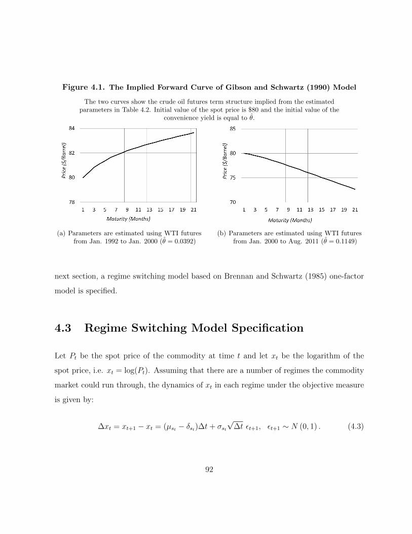
Figure 4.1. The Implied Forward Curve of Gibson and Schwartz (1990) Model
The two curves show the crude oil futures term structure implied from the estimatedparameters in Table 4.2. Initial value of the spot price is $80 and the initial value of the
convenience yield is equal to θ.
(a) Parameters are estimated using WTI futuresfrom Jan. 1992 to Jan. 2000 (θ = 0.0392)
(b) Parameters are estimated using WTI futuresfrom Jan. 2000 to Aug. 2011 (θ = 0.1149)
next section, a regime switching model based on Brennan and Schwartz (1985) one-factor
model is specified.
4.3 Regime Switching Model Specification
Let Pt be the spot price of the commodity at time t and let xt be the logarithm of the
spot price, i.e. xt = log(Pt). Assuming that there are a number of regimes the commodity
market could run through, the dynamics of xt in each regime under the objective measure
is given by:
∆xt = xt+1 − xt = (µst − δst)∆t+ σst√
∆t εt+1, εt+1 ∼ N (0, 1) . (4.3)
92

µst is the total expected return from holding one unit of the commodity. δst is the net
convenience yield, i.e the accrued benefits of holding one unit of the commodity in storage
minus the storage cost. σst is the volatility of the commodity price change. The values of
all three parameters are functions of which regime the market is in, which is indicated by
the subscript st where st is the process that determines which regime the market is in at
time t. This specification can be seen as an extension to the continuous time Brennan and
Schwartz (1985) model but with regime dependent parameters. Thus, we call this model
the Brennan and Schwartz regime switching (B&S-RS) model.
As in Hamilton (1994), st is modeled as an S-state discrete time Markov chain process
which is assumed to be independent of xt. The evolution of st is governed by the transitional
probability matrix which specifies the probability of switching from one regime to another.
In this study we are interested in the case where S = 2, i.e. there are only two regimes
in the market. For a two-state Markove chain, the transitional matrix under the objective
measure P is then given by:
ΠPt,t+1 =
πP(1,1) 1− πP
(1,1)
1− πP(2,2) πP
(2,2)
, (4.4)
where πP(i,i) is the P-measure probability to stay in regime i at t+ 1 given the market is in
regime i at t where i = 1, 2.
The B&S-RS model of this chapter is going to be compared with the Gibson and
Schwartz (1990) two-factor model (G&S). The discrete time version of G&S model can be
written as follows:
∆xt = (µ− δt)∆t+ σsε1,t (4.5)
∆δt = κ(θ − δt)∆t+ σδε2,t, (4.6)
93
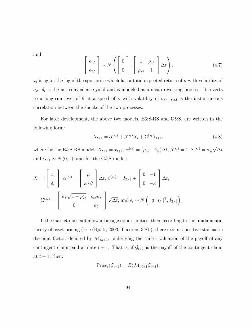
and ε1,t
ε2,t
∼ N
0
0
, 1 ρxδ
ρxδ 1
∆t
. (4.7)
xt is again the log of the spot price which has a total expected return of µ with volatility of
σx. δt is the net convenience yield and is modeled as a mean reverting process. It reverts
to a long-run level of θ at a speed of κ with volatility of σδ. ρxδ is the instantaneous
correlation between the shocks of the two processes.
For later development, the above two models, B&S-RS and G&S, are written in the
following form:
Xt+1 = α(st) + β(st)Xt + Σ(st)εt+1, (4.8)
where for the B&S-RS model: Xt+1 = xt+1, α(st) = (µst − δst)∆t, β(st) = 1, Σ(st) = σst√
∆t
and εt+1 ∼ N (0, 1); and for the G&S model:
Xt =
xt
δt
, α(st) =
µ
κ · θ
∆t, β(st) = I2×2 +
0 −1
0 −κ
∆t,
Σ(st) =
σx√
1− ρ2xδ ρxδσx
0 σδ
√∆t, and εt ∼ N(
[ 0 0 ]>, I2×2
).
If the market does not allow arbitrage opportunities, then according to the fundamental
theory of asset pricing ( see (Bjork, 2003, Theorem 3.8) ), there exists a positive stochastic
discount factor, denoted by Mt,t+1, underlying the time-t valuation of the payoff of any
contingent claim paid at date t + 1. That is, if Gt+1 is the payoff of the contingent claim
at t+ 1, then:
Pricet(Gt+1) = E(Mt,t+1Gt+1).
94
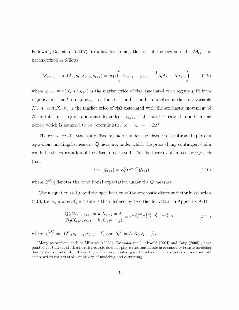
Following Dai et al. (2007), to allow for pricing the risk of the regime shift, Mt,t+1 is
parametrized as follows:
Mt,t+1 ≡M(Xt, st;Xt+1, st+1) = exp
(−rt,t+1 − γt,t+1 −
1
2ΛtΛ
>t − Λtεt+1
), (4.9)
where γt,t+1 ≡ γ(Xt, st; st+1) is the market price of risk associated with regime shift from
regime st at time t to regime st+1 at time t+1 and it can be a function of the state variable
Xt. Λt ≡ Λ(Xt, st) is the market price of risk associated with the stochastic movement of
Xt and it is also regime and state dependent. rt,t+1 is the risk free rate at time t for one
period which is assumed to be deterministic, i.e. rt,t+1 = r ·∆t5.
The existence of a stochastic discount factor under the absence of arbitrage implies an
equivalent martingale measure, Q measure, under which the price of any contingent claim
would be the expectation of the discounted payoff. That is, there exists a measure Q such
that:
Price(Gt+1) = EQt (e−r∆tGt+1), (4.10)
where EQt [·] denotes the conditional expectation under the Q measure.
Given equation (4.10) and the specification of the stochastic discount factor in equation
(4.9), the equivalent Q measure is then defined by (see the derivation in Appendix A.1):
Q(dXt+1, st+1 = k|Xt, st = j)
P(dXt+1, st+1 = k|Xt, st = j)= e−γ
(j,k)t,t+1−
12
Λ(j)t Λ
(j)>t −Λ
(j)t εt+1 , (4.11)
where γ(j,k)t,t+1 ≡ γ(Xt, st = j, st+1 = k) and Λ
(j)t ≡ Λ(Xt, st = j).
5Many researchers, such as Miltersen (2003), Carmona and Ludkovski (2004) and Tang (2009) , havepointed out that the stochastic risk free rate does not play a substantial role in commodity futures modelingdue to its low volatility. Thus, there is a very limited gain by introducing a stochastic risk free ratecompared to the resulted complexity of modeling and estimating.
95

Assuming γ(j,k)t,t+1 to be constant, i.e. γ
(j,k)t,t+1 = γ(j,k), then the regime switching probabili-
ties under Q are given by:
πQj,k = EQ
t [1st+1=k|st = j] = πPj,k · e−γ
(j,k)
, (4.12)
where 1st+1=k is an indicator function that equals to 1 if the subscript is true and zero
otherwise.
Moreover, assuming a constant market price of risk within each regime, i.e. Λ(st)t =(
Σ(st))−1
Λ(st), where Λ(st) is vector of constant within each regime, then it is shown in
Appendix A.2 that the behavior of Xt in the Q measure is given by:
Xt+1 = α(st) + β(st)Xt + Σ(st)εt+1, (4.13)
where: α(st) = α(st) − Λ(st).
For B&S-RS model, Λ(st) = λ(i)∆t, i = 1, 2, while for G&S model, since it is regime-
independent, Λ(st) = [λx∆t λδ∆t]>.
If the commodity is a traded asset, then absence of arbitrage implies that the total
expected return of holding a unit of the commodity should be equal to the risk-free rate.
This is due the fact that one can design a portfolio of the commodity and the derivatives
and choose the weights to eliminate the risk. Approximating the return on the commodity
by the difference in the logarithm6, i.e. ∆xt, this dynamic hedging implies:
EQ [∆xt|Jt, st = j] ≈ (r − δ(j))∆t, (4.14)
6 The approximating is reasonable for small time step. In this chapter, weekly data is used, i.e.∆t = 0.0192. Thus the error is negligible.
96

for B&S-RS one factor model, and
EQ [∆xt|Jt] ≈ (r − δt)∆t, (4.15)
for the G&S two factor model.
Thus, for the B&S-RS one factor model:
α(st) = (r − δ(st))∆t
and, for the G&S two factor model:
α(st) =
r
κ · θ − λδ
∆t
.
4.4 Futures Pricing
Denote Ft,n ≡ Fn(Xt, st) to be the futures price at time t of a unit of the commodity
delivered in n periods. A futures contract entered at time t has a payoff at time t + 1 of
Ft+1,n−1−Ft,n. Since, there is no payment at the inception at time t, this payoff must have
a price of zero, that is:
0 = e−r∆tEQt [Ft+1,n−1 − Ft,n] , (4.16)
which implies:
Ft,n = EQt [Ft+1,n−1] . (4.17)
97

Appendix A.3 shows that the futures price is an exponential affine function of the state
variable within each regime. Specifically:
Fn (Xt, st = j) = eA(j)n +BnXt , (4.18)
where for B&S-RS model:
A(j)n = Log
(S∑k=1
πjk · eA(k)n−1
)+Bn−1α
(j) +1
2Bn−1Σ(j)Σ(j)>B>n−1 (4.19)
Bn = Bn−1β, (4.20)
with A(i)0 = 0 for i = 1, 2 and B0 = 1. For the G&S model, S = 1 which implies:
An = An−1 +Bn−1α +1
2Bn−1ΣΣ>B>n−1 (4.21)
Bn = Bn−1β, (4.22)
with A0 = 0 and B0 = [1 0].
4.5 Estimation Methodology
As the focus of this study is on the crude oil markets, the B&S-RS one factor model can
be estimated using the time series of the crude oil spot price or, if not available, the first
contract of futures prices as a proxy. However, the parameters estimated this way would
not correspond to the Q measure which is the relevant measure for pricing contingent
claims. Moreover, using such methods, the convenience yield, δi where i = 1, 2, cannot be
identified.
98
In the bond pricing literature, where regime switching models have been studied ex-
tensively, several estimation methods have been proposed. Bansal and Zhou (2002) used
efficient method of moments (EMM). Dai et al. (2007) relied on maximum likelihood (ML)
which involves inverting equation (4.18) to extract the states vector, Xt, which has Gaus-
sian conditional likelihood. However, this requires one to chose a number of futures con-
tracts or to design a number of portfolios of futures contracts that is the same as the
number of factors to be extracted. The contracts choice or the portfolio weights are chosen
arbitrarily. Duffee and Stanton (2004) compared the performance of the three methods
in estimating affine term structure models: ML, EMM and methods based on Kalman
filter. They found that ML is a good method for simple term structure models and the
performance of EMM (a commonly used method for estimating complicated models) is
poor even in the simple term structure models. According to Duffee and Stanton (2004),
Kalman filtering procedure is found to be a tractable and reasonably accurate estimation
technique that they recommend in settings where ML is impractical.
Thus, in this chapter I use an extension to the Kalman filter for estimating the parame-
ters of the B&S-RS model proposed in Kim (1994). Blochlinger (2008) used this procedure
to estimate electricity price models in regime switching framework.
The Kalman filter is a recursive procedure for computing the optimal estimator of the
state vector at time t, based on the information available up to time t, and it enables
the estimate of the state vector to be continuously updated as new information becomes
available. When the disturbances and the initial state vector are normally distributed,
the Kalman filter enables the likelihood function to be calculated, which allows for the
estimation of any unknown parameters of the model and provides the basis for statistical
testing and model specification. For a detailed discussion of state space models and the
Kalman filter see Chapter 3 in Harvey (1989).
99
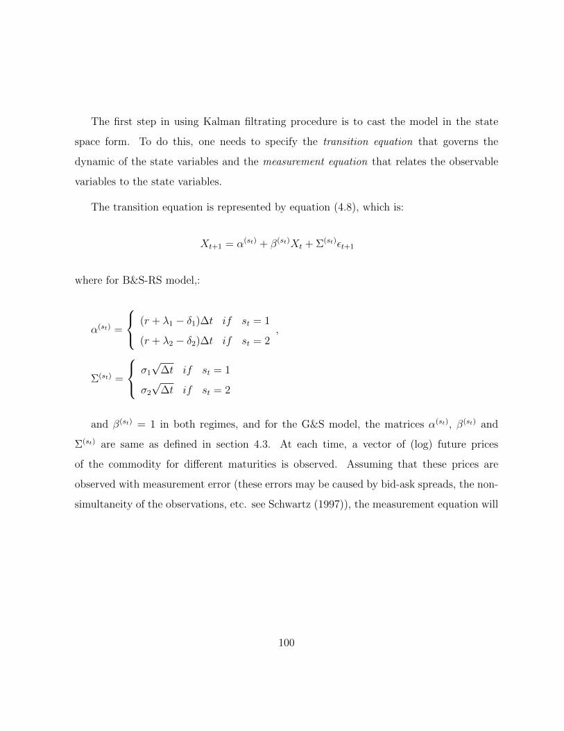
The first step in using Kalman filtrating procedure is to cast the model in the state
space form. To do this, one needs to specify the transition equation that governs the
dynamic of the state variables and the measurement equation that relates the observable
variables to the state variables.
The transition equation is represented by equation (4.8), which is:
Xt+1 = α(st) + β(st)Xt + Σ(st)εt+1
where for B&S-RS model,:
α(st) =
(r + λ1 − δ1)∆t if st = 1
(r + λ2 − δ2)∆t if st = 2,
Σ(st) =
σ1
√∆t if st = 1
σ2
√∆t if st = 2
and β(st) = 1 in both regimes, and for the G&S model, the matrices α(st), β(st) and
Σ(st) are same as defined in section 4.3. At each time, a vector of (log) future prices
of the commodity for different maturities is observed. Assuming that these prices are
observed with measurement error (these errors may be caused by bid-ask spreads, the non-
simultaneity of the observations, etc. see Schwartz (1997)), the measurement equation will
100
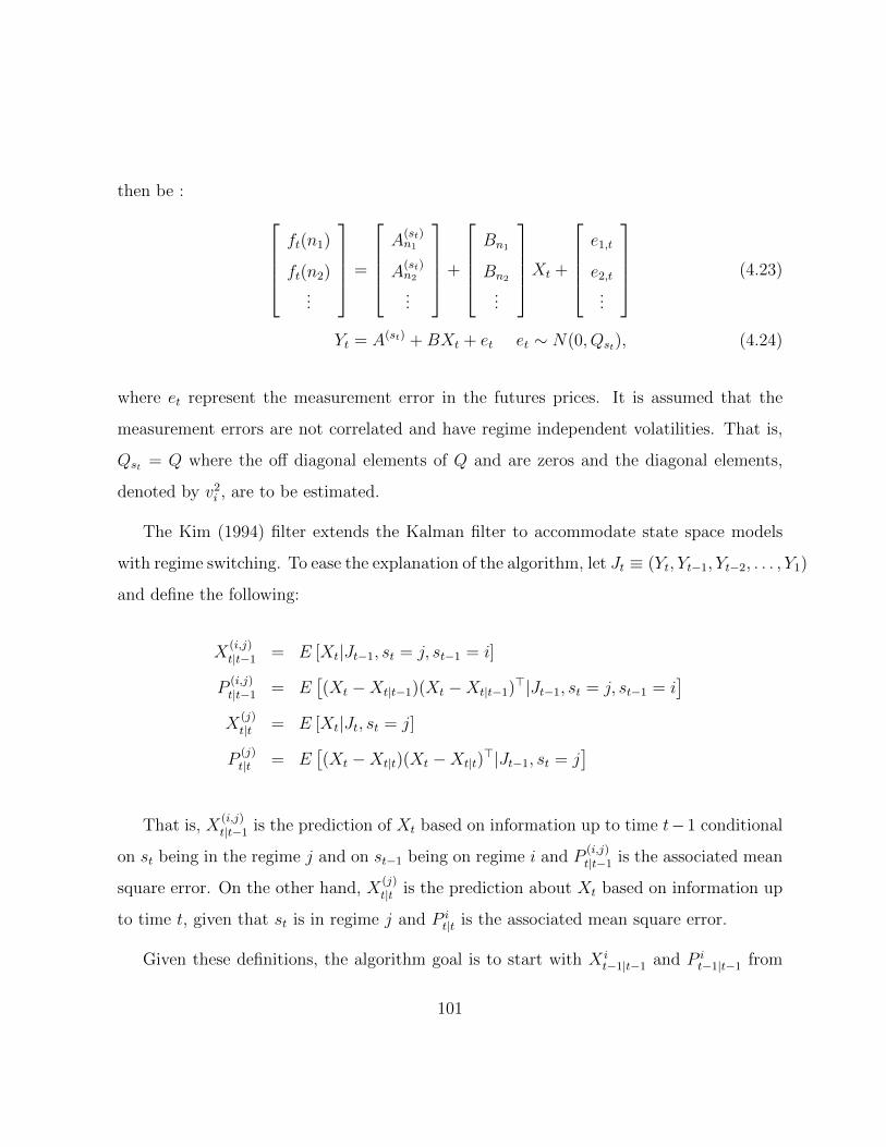
then be : ft(n1)
ft(n2)...
=
A
(st)n1
A(st)n2
...
+
Bn1
Bn2
...
Xt +
e1,t
e2,t
...
(4.23)
Yt = A(st) +BXt + et et ∼ N(0, Qst), (4.24)
where et represent the measurement error in the futures prices. It is assumed that the
measurement errors are not correlated and have regime independent volatilities. That is,
Qst = Q where the off diagonal elements of Q and are zeros and the diagonal elements,
denoted by v2i , are to be estimated.
The Kim (1994) filter extends the Kalman filter to accommodate state space models
with regime switching. To ease the explanation of the algorithm, let Jt ≡ (Yt, Yt−1, Yt−2, . . . , Y1)
and define the following:
X(i,j)t|t−1 = E [Xt|Jt−1, st = j, st−1 = i]
P(i,j)t|t−1 = E
[(Xt −Xt|t−1)(Xt −Xt|t−1)>|Jt−1, st = j, st−1 = i
]X
(j)t|t = E [Xt|Jt, st = j]
P(j)t|t = E
[(Xt −Xt|t)(Xt −Xt|t)
>|Jt−1, st = j]
That is, X(i,j)t|t−1 is the prediction of Xt based on information up to time t−1 conditional
on st being in the regime j and on st−1 being on regime i and P(i,j)t|t−1 is the associated mean
square error. On the other hand, X(j)t|t is the prediction about Xt based on information up
to time t, given that st is in regime j and P it|t is the associated mean square error.
Given these definitions, the algorithm goal is to start with X it−1|t−1 and P i
t−1|t−1 from
101

the previous step to produce X it|t and P i
t|t of the current step using the above model and
the current observation of time t. Specifically, it goes by:
X(i,j)t|t−1 = αiX
(i)t−1|t−1 (4.25)
P(i,j)t|t−1 = αiP
(i)t−1|t−1α
>i + ΣiΣ
>i (4.26)
η(i,j)t|t−1 = Yt − (Aj +BjX
(i,j)t|t−1) (4.27)
H(i,j)t = BjP
(i,j)t|t−1B
>j +Qj (4.28)
K(i,j)t = P
(i,j)t|t−1B
>j
[H
(i,j)t
]−1
(4.29)
X(i,j)t|t = X
(i,j)t|t−1 +K
(i,j)t η
(i,j)t|t−1 (4.30)
P(i,j)t|t = (I −K(i,j)
t )P(i,j)t|t−1. (4.31)
These step constitutes the Kalman filtering procedure and given the normality assump-
tion of the pricing errors, the likelihood of observing Yt conditional on Jt−1 and on st = j
and st−1 = i can be evaluated as follows:
f(Yt|st−1 = i, st = j, Jt) = (2π)−N/2|H(i,j)t |−1/2exp(−1
2η
(i,j)>t|t−1 H
(i,j)t η
(i,j)t|t−1), (4.32)
where N is the size of Xt. For Gibson and Schwartz (1990) model, where the model is
regime independent (i.e. S = 1), the above likelihood reduced to f(Yt|Jt−1).
However, if the number of the regimes is S > 1 (in our case S = 2), then the results
of the above filtration procedure is S2 predictions, X(i,j)t|t , and S2 associated forecast er-
rors, P(i,j)t|t . Thus, each iteration would require S-fold of cases to consider. Kim (1994)
suggested the following approximation, in each iteration, to collapse the S2 forecasts and
102
their associated forecast errors to only S cases:
X(j)t|t =
∑Si=1 Pr [st−1 = i, st = j|Jt] ·X(i,j)
t|t
Pr [st = j|Jt](4.33)
P(j)t|t =
∑Si=1 Pr [st−1 = i, st = j|Jt] ·
(P
(i,j)t|t + (X
(j)t|t −X
(i,j)t|t )(X
(j)t|t −X
(i,j)t|t )>
)Pr [st = j|Jt]
. (4.34)
Kim (1994) gives the details behind this approximation of this procedure. The outputs
X(j)t|t and P
(j)t|t are then used as inputs to the Kalman filtration procedure in the next step.
To achieve this recursive procedure, one needs to calculate the probabilities terms
appearing in equations (4.33) and (4.34). Kim (1994) suggested to use the Hamilton
(1994) procedure to obtain these probabilities recursively. This procedure is explained in
detail in Appendix A.4.
As shown in Appendix A.4, as a by product of the Hamilton (1994) filtration procedure,
the conditional likelihood of each iteration, f(Yt;ψ|Jt−1) is obtained, where ψ is the set of
parameters to be estimated.
Having the likelihood of each observation, the parameters of the two models can then
be estimated by maximizing the likelihood of the sample, that is:
ψ = arg maxψ
T∑t=1
log(f(Yt;ψ|Jt−1)).
4.6 Data Description
To estimate the parameters of the two models, weekly data of West Texas Intermediate
(WTI) crude oil futures are used. WTI crude oil futures contracts for more than four years
103

Figure 4.2. Crude Oil Price and Return Series
-0.4
-0.2
0
0.2
0.4
0.6
0.8
1
1.2
0
20
40
60
80
100
120
140
160
Right scale is for WTI oil spot price, left scale is for its log return and shaded areas arefor the periods of contango markets.
104
maturities are traded in New York Mercantile Exchange (NYMEX). WTI futures contracts
are very liquid and are among the most traded commodity futures worldwide. Data from
January 1992 to the August of 2011 has been obtained from Datastream and the Energy
Information Administration (US Department of Energy). For the risk free rate, the average
of the 3 months U.S. treasury bill is used.
To construct continuous series of futures prices, following the literature, futures prices
are sorted each week according to the contract horizon with "first month" contract being
the contract with the earliest delivery date, the "second month" contract being the contract
with the next earliest delivery date, etc. Each contract will switch to the next one just
before it expires7
The performance of our specification of the B&S-RS one-factor model is compared
with the G&S two-factor model. The estimation and performance analysis are done for
the whole sample period and for two sub-periods, namely: from January 1992 to January
2000 and from January 2000 to August 2011.
Table 4.1 reports descriptive statistics for the weekly returns of the spot, 6th, 12th, 17th
and 20th months contracts: unconditionally and conditional on the slope of the futures
term structure being positive or negative. The table shows that crude oil market visits
backwardation regime and contango regime half of the time in the whole sample period
and in the two sub-samples. Moreover, periods of backwardation generate higher returns.
The market has higher volatility when being in contango than the case when it is being
in backwardation. It is also clear that volatility declines with maturity; an observation
known in futures prices literature as Samuelson’s effect.
7For WTI, trading in the current delivery month ceases on the third business day prior to thetwenty-fifth calendar day of the month preceding the delivery month. More details can be seen inhttp://www.cmegroup.com.
105
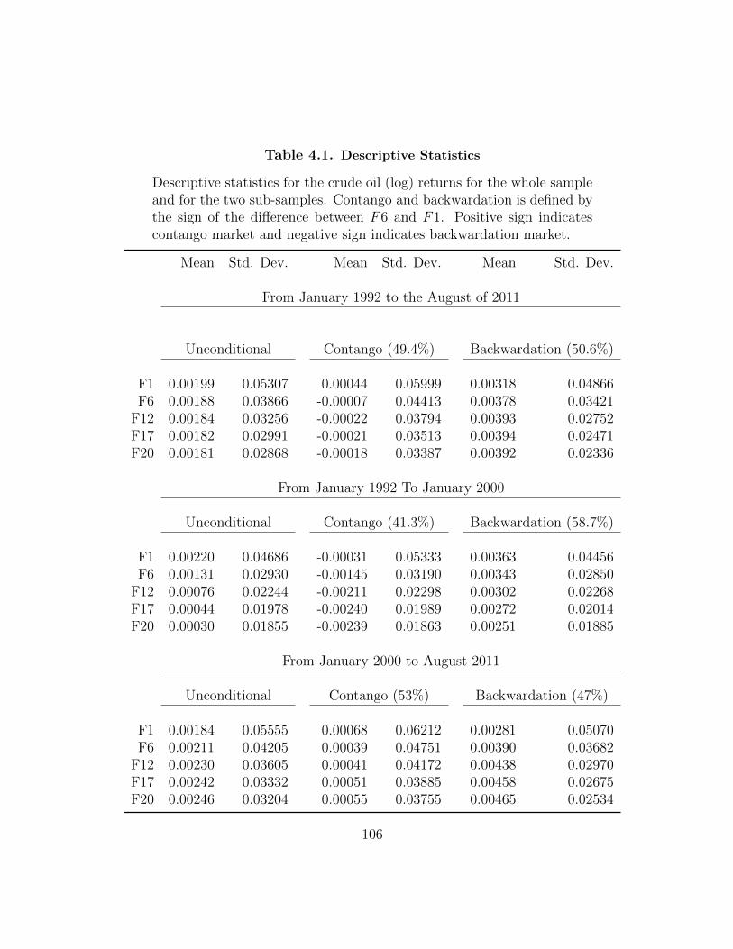
Table 4.1. Descriptive Statistics
Descriptive statistics for the crude oil (log) returns for the whole sampleand for the two sub-samples. Contango and backwardation is defined bythe sign of the difference between F6 and F1. Positive sign indicatescontango market and negative sign indicates backwardation market.
Mean Std. Dev. Mean Std. Dev. Mean Std. Dev.
From January 1992 to the August of 2011
Unconditional Contango (49.4%) Backwardation (50.6%)
F1 0.00199 0.05307 0.00044 0.05999 0.00318 0.04866F6 0.00188 0.03866 -0.00007 0.04413 0.00378 0.03421
F12 0.00184 0.03256 -0.00022 0.03794 0.00393 0.02752F17 0.00182 0.02991 -0.00021 0.03513 0.00394 0.02471F20 0.00181 0.02868 -0.00018 0.03387 0.00392 0.02336
From January 1992 To January 2000
Unconditional Contango (41.3%) Backwardation (58.7%)
F1 0.00220 0.04686 -0.00031 0.05333 0.00363 0.04456F6 0.00131 0.02930 -0.00145 0.03190 0.00343 0.02850
F12 0.00076 0.02244 -0.00211 0.02298 0.00302 0.02268F17 0.00044 0.01978 -0.00240 0.01989 0.00272 0.02014F20 0.00030 0.01855 -0.00239 0.01863 0.00251 0.01885
From January 2000 to August 2011
Unconditional Contango (53%) Backwardation (47%)
F1 0.00184 0.05555 0.00068 0.06212 0.00281 0.05070F6 0.00211 0.04205 0.00039 0.04751 0.00390 0.03682
F12 0.00230 0.03605 0.00041 0.04172 0.00438 0.02970F17 0.00242 0.03332 0.00051 0.03885 0.00458 0.02675F20 0.00246 0.03204 0.00055 0.03755 0.00465 0.02534
106

4.7 Estimation Results
Table 4.2 shows the results of the Kim filter estimation and Figure 4.3 shows the implied
term structure of the futures prices for the whole sample and the two sub-samples. For
comparison purposes, the futures term structures implied by the Gibson and Schwartz
(1990) two-factor model for the three periods are included.
Regarding the estimated parameters of B&S-RS model, all the parameters are signifi-
cant except those for the market price of risk8.
Regime one is characterized by negative convenience (δ1) and higher volatility (σ1).
On the other hand, regime two is characterized by positive convenience (δ2) and lower
volatility (σ2). It is clear from the figure that the first regime corresponds to a positive
slope of the futures term structure while the second regime corresponds to a negative slope
of the futures term structure. The volatility estimates of both regimes are high reflecting
the higher variability of crude oil markets as it is the case in energy markets and commodity
markets in general (see for example Deaton and Laroque (1996)). However, this result is
at odds with the theory of storage prediction which asserts that higher convenience yield
is associated with low level of inventory and high volatility
The classification of observation into the two regimes coincides with the observed slope
of the futures term structure as shown in figure 4.4. There are two methods in literature
8Standard test statistics (such as Lagrange Multiplier, Likelihood Ratio and Wald test statistics) cannotbe used to test whether there is one regime or two regimes in the data. This is because the parametersrelated to the second regime are not identified under the null of no regime-switching. In this case, stan-dard asymptotic distribution theory cannot be applied and the usual test statistics are not chi-squareddistributed asymptotically. Hansen (1996) proposed a standardized likelihood ratio statistic to conduct thetest in such situations. The idea is to concentrate the identified parameters out of the likelihood functionand take the supremum of the concentrated likelihood function over the possible unidentified parametersafter standardizing it. The optimization can be done by using a grid search across plausible values for thenuisance parameters which is computationally extremely expensive unless the model is very simple.
107
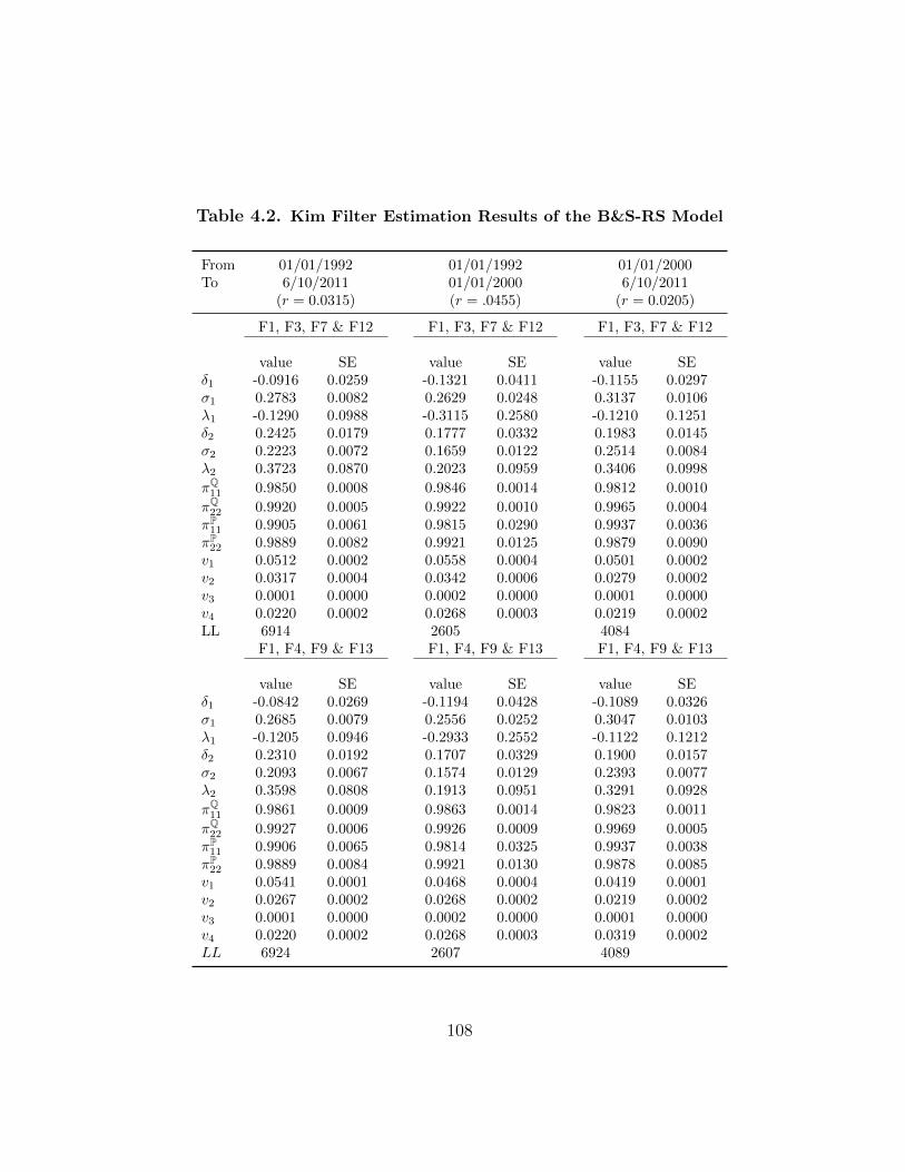
Table 4.2. Kim Filter Estimation Results of the B&S-RS Model
From 01/01/1992 01/01/1992 01/01/2000To 6/10/2011 01/01/2000 6/10/2011
(r = 0.0315) (r = .0455) (r = 0.0205)
F1, F3, F7 & F12 F1, F3, F7 & F12 F1, F3, F7 & F12
value SE value SE value SEδ1 -0.0916 0.0259 -0.1321 0.0411 -0.1155 0.0297σ1 0.2783 0.0082 0.2629 0.0248 0.3137 0.0106λ1 -0.1290 0.0988 -0.3115 0.2580 -0.1210 0.1251δ2 0.2425 0.0179 0.1777 0.0332 0.1983 0.0145σ2 0.2223 0.0072 0.1659 0.0122 0.2514 0.0084λ2 0.3723 0.0870 0.2023 0.0959 0.3406 0.0998
πQ11 0.9850 0.0008 0.9846 0.0014 0.9812 0.0010
πQ22 0.9920 0.0005 0.9922 0.0010 0.9965 0.0004πP11 0.9905 0.0061 0.9815 0.0290 0.9937 0.0036πP22 0.9889 0.0082 0.9921 0.0125 0.9879 0.0090v1 0.0512 0.0002 0.0558 0.0004 0.0501 0.0002v2 0.0317 0.0004 0.0342 0.0006 0.0279 0.0002v3 0.0001 0.0000 0.0002 0.0000 0.0001 0.0000v4 0.0220 0.0002 0.0268 0.0003 0.0219 0.0002LL 6914 2605 4084
F1, F4, F9 & F13 F1, F4, F9 & F13 F1, F4, F9 & F13
value SE value SE value SEδ1 -0.0842 0.0269 -0.1194 0.0428 -0.1089 0.0326σ1 0.2685 0.0079 0.2556 0.0252 0.3047 0.0103λ1 -0.1205 0.0946 -0.2933 0.2552 -0.1122 0.1212δ2 0.2310 0.0192 0.1707 0.0329 0.1900 0.0157σ2 0.2093 0.0067 0.1574 0.0129 0.2393 0.0077λ2 0.3598 0.0808 0.1913 0.0951 0.3291 0.0928
πQ11 0.9861 0.0009 0.9863 0.0014 0.9823 0.0011
πQ22 0.9927 0.0006 0.9926 0.0009 0.9969 0.0005πP11 0.9906 0.0065 0.9814 0.0325 0.9937 0.0038πP22 0.9889 0.0084 0.9921 0.0130 0.9878 0.0085v1 0.0541 0.0001 0.0468 0.0004 0.0419 0.0001v2 0.0267 0.0002 0.0268 0.0002 0.0219 0.0002v3 0.0001 0.0000 0.0002 0.0000 0.0001 0.0000v4 0.0220 0.0002 0.0268 0.0003 0.0319 0.0002LL 6924 2607 4089
108
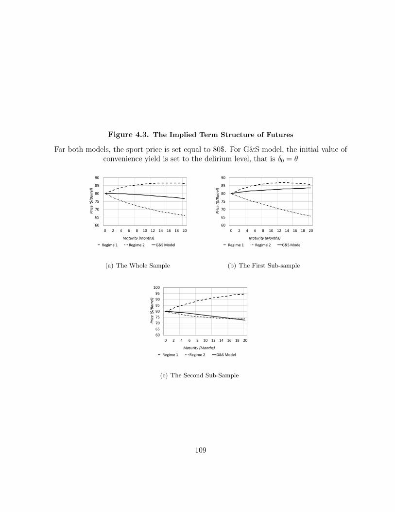
Figure 4.3. The Implied Term Structure of Futures
For both models, the sport price is set equal to 80$. For G&S model, the initial value ofconvenience yield is set to the delirium level, that is δ0 = θ
60
65
70
75
80
85
90
0 2 4 6 8 10 12 14 16 18 20
Pri
ce (
$/B
arr
el)
Maturity (Months)
Regime 1 Regime 2 G&S Model
(a) The Whole Sample
60
65
70
75
80
85
90
0 2 4 6 8 10 12 14 16 18 20
Pri
ce (
$/B
arr
el)
Maturity (Months)
Regime 1 Regime 2 G&S Model
(b) The First Sub-sample
60
65
70
75
80
85
90
95
100
0 2 4 6 8 10 12 14 16 18 20
Pri
ce (
$/B
arr
el)
Maturity (Months)
Regime 1 Regime 2 G&S Model
(c) The Second Sub-Sample
109
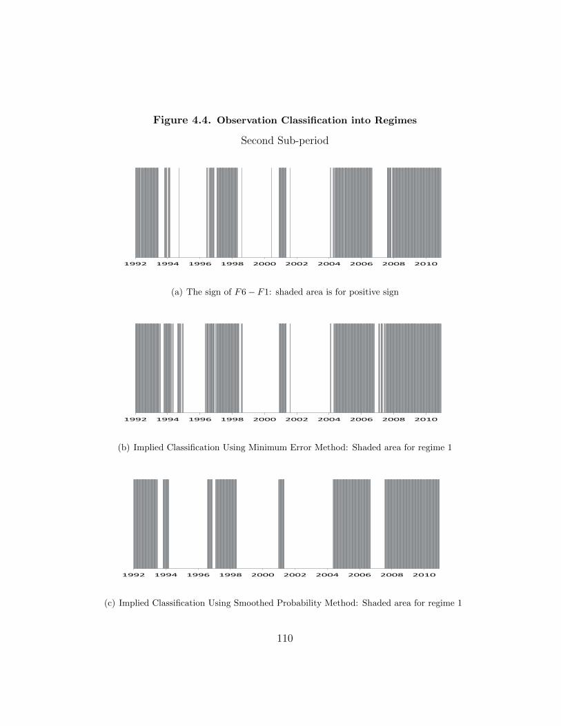
Figure 4.4. Observation Classification into Regimes
Second Sub-period
1992 1994 1996 1998 2000 2002 2004 2006 2008 2010
(a) The sign of F6− F1: shaded area is for positive sign
1992 1994 1996 1998 2000 2002 2004 2006 2008 2010
(b) Implied Classification Using Minimum Error Method: Shaded area for regime 1
1992 1994 1996 1998 2000 2002 2004 2006 2008 2010
(c) Implied Classification Using Smoothed Probability Method: Shaded area for regime 1
110
to classify the observation into its regime. The first one is to use the smoothed regime
probabilities, i.e. Pr[st = j|JT ]. If Pr[st = j|JT ] > .5, then t is classified into regime
j. This method was suggested by Hamilton (1994). The other method is to compare the
fitted prices of each regime with the actual prices at each time and classify the observation
to the regime that has the least error. That is, if the fitted futures price at time t for
regime i is closer to the actual price, then, st is set to equal i. This method has been used
by Bansal and Zhou (2002).
From figure 4.4, comparing 4.4(a) with 4.4(b) and 4.4(c), it is clear that the first regime
corresponds to the market having positive slope while the second one corresponds to the
market having a negative slop. In other words, the first regime shows the market when
being in contango and the second regime shows the market when being in backwardation.
Transitional probabilities, πP11 and πP
22, in both regimes reflect the persistence of each
regime. Note that the reported values are the probabilities to switch between the two
regimes in one week. The values are very high for both regimes because the a period of
one week is too short to allow for switching. To make a clearer picture, the corresponding
annual transitional probabilities are calculated as follows : 0.9905 1− 0.9905
1− 0.9889 0.9889
(52)
=
0.6951 0.3049
0.3563 0.6437
.That is, the probability to stay in the same regime after one year is 0.6951 for regime 1 and
0.6437 for regime 2. The result shows that both regimes are highly persistence. Moreover,
the market stays slightly longer in the first regime where it has lower volatility and positive
convenience yield. The recent persistence in regime one at the end of the financial crisis
and afterward, as shown in Figure 4.4, contributes to the fact that πP1,1 is slightly higher
than πP22 although the market visits regime two more than regime one in the estimation
period, as shown in Table 4.1.
111

Figure 4.5. The Impact of the Market Price of Regime Switching Risk
The transitional probabilities in the pricing measure, measure Q, is given by πQ11 and
πQ22. These estimates reflects how the market reacts to the risk of the regime shift. Again,
the annual transitional probabilities are calculated as follows: 0.9850 1− 0.9850
1− 0.9920 0.9920
(52)
=
0.5423 0.4577
0.2441 0.7559
.These number shows that the risk of switching from regime one to regime two in one year
is higher in Q than in the actual measure P (0.4577 > 0.3049). On the other hand, the risk
of switching from regime two to regime one in one year is lower in Q than in the actual
measure P (0.2441 < 0.3563). If the market is currently in regime one, where futures prices
are higher than the spot price, risk-averse market participants set the switching risk (the
probability that futures prices will drop lower than the spot price) to be higher than actual
risk. On the other hand, if the market is currently in regime two, where futures prices
112
are lower than the spot price, they set the switching risk (the probability that futures
prices will jump up above the spot price) to be lower than the actual risk. In both cases,
they achieve that by setting futures prices lower than what is expected to be if they are
risk neutral in term of regime shift. Figure 4.5 explains this fact by depicting the implied
futures term structure in each regime using the transitional probabilities of both measures.
it shows that risk averse market participants, to account for the risk of regime shift, set
the futures prices lower than what spot price is expected to be at expiry. Moreover, the
reduction increases as the maturity of the futures contract increases.
Table 4.2 also shows that the first regime has a negative market price of risk, λ1 =
−0.129, while the second regime has a high and a positive market price of risk, λ2 = 0.37.
That is, in the first regime, market participants trade futures contracts at higher prices than
expected at maturity as a reward of bearing the price risk. On the other hand, in the second
regime, they trade futures contracts at lower prices than expected at maturity. This is also
confirmed by the observation from Table 4.1 where the returns are negative in contango
(regime one according to the estimates of our model) and positive in backwardation (regime
two according to the estimates of our model). However, the standard errors of the market
price of risk (MPR) parameters, λ1 and λ2, are relatively high compared with the other
parameters. The reason for that is, as explained in Schwartz and Smith (2000), the MPR
parameters cannot be directly identified from futures prices.
Table 4.2 shows that the the same pattern of results appears also in the two sub-samples
reflecting the stability of the parameters.
113
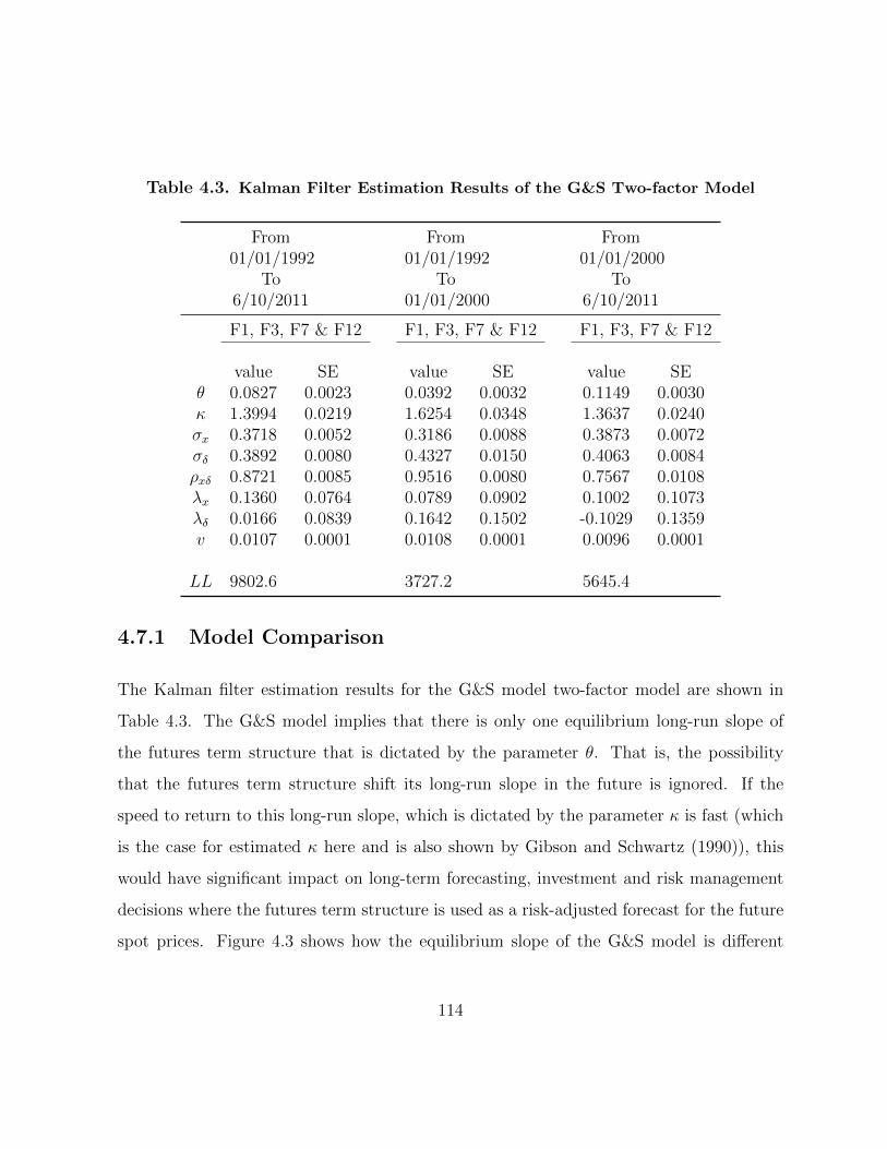
Table 4.3. Kalman Filter Estimation Results of the G&S Two-factor Model
From01/01/1992
To6/10/2011
From01/01/1992
To01/01/2000
From01/01/2000
To6/10/2011
F1, F3, F7 & F12 F1, F3, F7 & F12 F1, F3, F7 & F12
value SE value SE value SEθ 0.0827 0.0023 0.0392 0.0032 0.1149 0.0030κ 1.3994 0.0219 1.6254 0.0348 1.3637 0.0240σx 0.3718 0.0052 0.3186 0.0088 0.3873 0.0072σδ 0.3892 0.0080 0.4327 0.0150 0.4063 0.0084ρxδ 0.8721 0.0085 0.9516 0.0080 0.7567 0.0108λx 0.1360 0.0764 0.0789 0.0902 0.1002 0.1073λδ 0.0166 0.0839 0.1642 0.1502 -0.1029 0.1359v 0.0107 0.0001 0.0108 0.0001 0.0096 0.0001
LL 9802.6 3727.2 5645.4
4.7.1 Model Comparison
The Kalman filter estimation results for the G&S model two-factor model are shown in
Table 4.3. The G&S model implies that there is only one equilibrium long-run slope of
the futures term structure that is dictated by the parameter θ. That is, the possibility
that the futures term structure shift its long-run slope in the future is ignored. If the
speed to return to this long-run slope, which is dictated by the parameter κ is fast (which
is the case for estimated κ here and is also shown by Gibson and Schwartz (1990)), this
would have significant impact on long-term forecasting, investment and risk management
decisions where the futures term structure is used as a risk-adjusted forecast for the future
spot prices. Figure 4.3 shows how the equilibrium slope of the G&S model is different
114

across the two subperiods which reflect the instability of θ, the parameter that dictates the
equilibrium slope of the futures term structure.
In term of comparing the performance of B&S-RS model with the G&S model in fitting
the futures term structure, figure 4.6 shows that although the G&S model outperforms
B&S-RS model for short-term maturities, B&S-RS model outperforms the G&S model for
long-term maturities. Figures 4.7 and 4.8 show the same pattern for the two sub-periods.
This result is an implication of the assumption of the G&S model that the convenience
yield reverts to only one equilibrium level which implies that the futures term structure
should revert to one slope all the time.
4.7.2 The Impact of the Transitional Probabilities
Within the framework of our regime switching model, the transitional probabilities πQ11 and
πQ22 have an important role in shaping the term structure of the futures prices. Figure 9
shows how the term structure changes with different values of the transitional probabilities
and for each regime.
For easy presentation, denote p = πQ11 and q = πQ
22. Consider the market to be currently
in regime one where the slope of the forward curve is positive. Figure 4.9(a) shows that as p
decrease relative to q, the far end of the curve bends down. This is because the probability
to be in regime 2, which is characterized by having negative slope, is now higher. Figure
4.9(b) shows that as q decreases, the far end of the curve bends up because the probability
to be in regime 1, which is characterized by having positive slope, is now higher. However,
the effect of changing q is much smaller than the effect of changing p because the market is
now in regime one. The same pattern is also seen when the market is currently in regime
2 where the forward curve has a negative slope. figure 4.9(d) shows that as q decrease
115
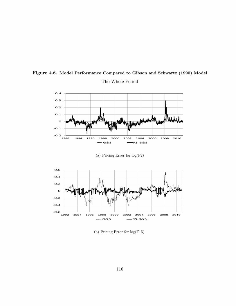
Figure 4.6. Model Performance Compared to Gibson and Schwartz (1990) Model
Tho Whole Period
-0.2
-0.1
0
0.1
0.2
0.3
0.4
1992 1994 1996 1998 2000 2002 2004 2006 2008 2010
G&S RS-B&S
(a) Pricing Error for log(F2)
-0.6
-0.4
-0.2
0
0.2
0.4
0.6
1992 1994 1996 1998 2000 2002 2004 2006 2008 2010
G&S RS-B&S
(b) Pricing Error for log(F15)
116
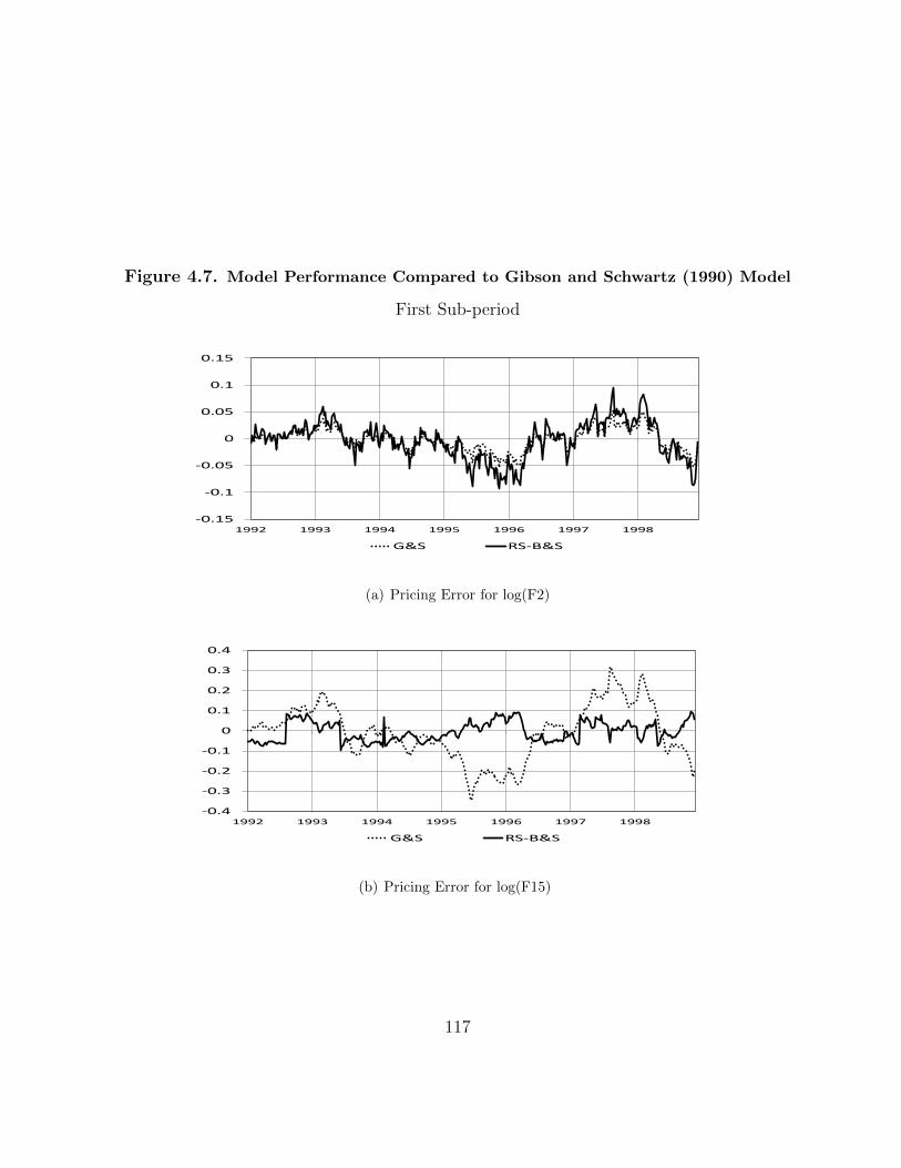
Figure 4.7. Model Performance Compared to Gibson and Schwartz (1990) Model
First Sub-period
-0.15
-0.1
-0.05
0
0.05
0.1
0.15
1992 1993 1994 1995 1996 1997 1998
G&S RS-B&S
(a) Pricing Error for log(F2)
-0.4
-0.3
-0.2
-0.1
0
0.1
0.2
0.3
0.4
1992 1993 1994 1995 1996 1997 1998
G&S RS-B&S
(b) Pricing Error for log(F15)
117
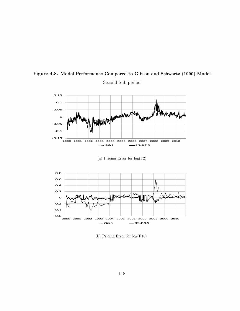
Figure 4.8. Model Performance Compared to Gibson and Schwartz (1990) Model
Second Sub-period
-0.15
-0.1
-0.05
0
0.05
0.1
0.15
2000 2001 2002 2003 2004 2005 2006 2007 2008 2009 2010
G&S RS-B&S
(a) Pricing Error for log(F2)
-0.6
-0.4
-0.2
0
0.2
0.4
0.6
0.8
2000 2001 2002 2003 2004 2005 2006 2007 2008 2009 2010
G&S RS-B&S
(b) Pricing Error for log(F15)
118
relative to p, the far end of the curve bends up because the probability to be in regime 1,
which has positive slope, is now higher. Figure 4.9(c) shows that as p increases, the far
end of the curve bends up because the probability to be in regime 1. However, the effect
of changing p is much smaller than the effect of changing q because the market is currently
in regime two.
The estimates of the transitional probabilities are assumed to be exogenous and con-
stant and thus the estimated transitional probabilities reflect the persistence of the regimes
during the estimation period, which is not necessary true for future periods. One way to
improve the regime switching model prediction is to have time varying transitional proba-
bilities. An appealing feature of B&S-RS model of this study is that the regimes that the
market runs through correspond to the slope of futures term structure. A large amount
of research has been conducted to explain the factors behind the changes in the shape of
the futures term structure, especially what factors make the market being in contango or
backwardation. Examples of such factors are: inventory level and volatility of the mar-
ket ( see Williams and Wright (1991) and Deaton and Laroque (1996)); hedging pressure,
the net hedging position of short and long sides of the market, (see Roon et al. (2000),
Dinceler et al. (2003) and Gorton et al. (2007)). These factors can be exploited to improve
the estimation about the probability of switching from a regime to another.
4.8 Concluding Remarks
In this chapter, we exploit regime switching models to study the movement in the crude
oil futures term structures. In particular, we extend Brennan and Schwartz (1985) one-
factor model to account for shifts in in the futures term structure between contango and
backwardation and the reverse in discrete time setting. We allow for the regime shift
119
risk as well as the market price risk. Moreover, we derive a closed from solution for the
futures prices and used an extension to the Kalman filter suggested by Kim (1994) to
estimate the model parameters in discrete time. Compared to the performance of the
Gibson and Schwartz (1990) two-factor, the regime switching one-factor model of this
study did a reasonable job. In particular, the model outperforms Gibson and Schwartz
(1990) model for fitting the prices of longer maturities contracts. Moreover, it is found
that the transitional probabilities played an important role in shaping the futures term
structure implied by the model.
As a future extension to the model, one might add more state factors other than the
spot price movement. In this case, one needs to be careful in choosing the added factors
as an important assumption in deriving the futures formula is that the state variables
are independent from the Markov chain process governing the regime switching. Another
direction is to test the improvement of the model when the transitional probabilities are
endogenous and using the variables that the literature finds have explanation power in
determining the shape of the futures term structure such as inventory level and the net
hedging position.
120

Figure 4.9. The Impact of the Transitional Probabilities
For easing the display of the graphs, πQ11 = p and πQ
22 = q
60
65
70
75
80
85
90
95
100
1 3 5 7 9 11 13 15 17 19 21
p= 0.99
p= 0.95
(a) Regime One: p changes and q is at estimatedvalue
60
65
70
75
80
85
90
95
100
1 3 5 7 9 11 13 15 17 19 21
q= 0.99
q= 0.95
(b) Regime One: q changes and p is at estimatedvalue
60
65
70
75
80
85
90
95
100
1 3 5 7 9 11 13 15 17 19 21
p= 0.99
p= 0.95
(c) Regime Two: p changes and q is at estimatedvalue
60
65
70
75
80
85
90
95
100
1 3 5 7 9 11 13 15 17 19 21
q= 0.99
q= 0.95
(d) Regime Two: q changes and p is at estimatedvalue
121

Chapter 5
Conclusion
This thesis attempts to contribute to the existing understanding of risk management in
crude oil markets through three essays. In the first essay (chapter 2), the valuation of an
oil sands project is studied using real options approach. Oil sands production consumes
substantial amount of natural gas during extracting and upgrading. Natural gas prices are
known to be stochastic and highly volatile which introduces a significant stochastic compo-
nent in the extraction cost. The essay studies the impact of this stochastic component on
the value of an oil sands project and its optimal operation. Before studying the valuation
problem, the essay investigated the co-movement of crude oil and natural gas prices. It
is found that although there are economic links between the two commodities, the em-
pirical evidence in detecting a long-run relationship is weak especially if one incorporates
the recent divergence in the two price series. Accordingly, in modeling the dynamics of
the two prices, two models are proposed, one incorporates a long-run link between the
two markets while the other has no such link. The valuation problem is solved using the
Least Square Monte Carlo (LSMC) method proposed by Longstaff and Schwartz (2001)
122
for valuing American options. The valuation results show that incorporating a long-run
relationship between the two markets is a very crucial decision in the value of the project
and in its optimal operation. The chapter shows that ignoring this long-run relationship
makes the optimal policy sensitive to the dynamics of natural gas prices. On the other
hand, incorporating this long-run relationship makes the dynamics of natural gas price
process have a very low impact on valuation and the optimal operating policy. Natural gas
is the primary fuel source for the oil sands industry. An interesting extension is to study
the impact of having a new technology that replaces the natural gas as the source of fuel
in oil sands extraction and upgrading. Moreover, natural gas prices have fallen recently
due to the emergence of a large supply from gas shale deposits. An interesting extension
is to study the potential impact of this development on the volatility of natural gas prices,
on the co-movement of natural gas and crude oil prices, on the search for other alternative
fuel sources and in turn on the value of an oil sands project.
In the second essay (chapter 3), the relationship between the slope of the futures term
structure and volatility in the crude oil market is investigated using a measure of the slope
based on principal component analysis (PCA) proposed by Borovkova (2006). The ad-
vantage of using PCA is that all futures prices are used in calculating the slope of the
forward curve. I show in the essay that this slope measure has more power to predict the
market volatility than the measures commonly used in literature. The essay begins by
reviewing the main theories of the relation between spot and futures prices and consider-
ing the implication of each theory on the relation between the slope of the forward curve
and volatility. Both the literature in commodities price modeling and the literature in
exhaustible resources pricing contain theories which have some implications for the equi-
librium state of this relationship. Five main theories are presented and their implications
are compared. After that, the diagonal VECH model of Bollerslev et al. (1988) was used
123

to analyze the relationship between of the forward curve slope and the variances of the
spot and futures prices and the covariance between them. The results show that there is a
significant quadratic relationship. That is, the variances are expected to be higher when-
ever the slope is steeper regardless of its sign. Moreover, the essay shows that exploiting
this relation improves the hedging performance using futures contracts.
The third essay (chapter 4) attempts to model the spot price process of crude oil using
the notion of convenience yield in a regime switching framework. The notion of convenience
yield plays a central role in commodities price modeling as it derives the relationship
between futures and spot prices in the commodities markets. Unlike the existing studies,
which assume the convenience yield to have either a constant value or to have a stochastic
behavior with mean reversion to one equilibrium level, the model of this essay extends the
Brennan and Schwartz (1985) model to allows for regime switching in the convenience yield
along with the other parameters. In the essay, a closed form solution for the futures price
is derived. The parameters are estimated using an extension to the Kalman filter proposed
by Kim (1994). The regime switching one-factor model of this study did a reasonable job.
In particular, the model outperforms the Gibson and Schwartz (1990) two factor model for
fitting the prices of longer maturities contracts. Moreover, I found that the transitional
probabilities played an important role in shaping the futures term structure implied by
the model. As a future extension to the model, more state factors other than the spot
price movement might be added. In this case, one needs to be careful in choosing the
added factors as an important assumption in deriving the futures formula is that the state
variables are independent from the Markov chain process governing the regime switching.
Moreover, the model can be improved by relaxing the assumption of constant traditional
probabilities. Better results might be obtained if the transitional probabilities are time
varying. However, this will be at the cost of making the model more complex in terms of
124

finding a closed form solution for the futures price and in terms of estimation
125
Bibliography
Alizadeh, A. H., Nomikos, N. K., and Pouliasis, P. K. (2008). A Markov regime switching
approach for hedging energy commodities. Journal of Banking and Finance, 32:1970–
1983.
Anson, M. J. (2002). The Handbook of Alternative Assets. The Frank J. Fabozzi Series.
John Wiley & Sons, Inc.
Armstrong, M., Galli, A., Bailey, W., and Couet, B. (2004). Incorporating technical
uncertainty in real option valuation of oil projects. Journal of Petroleum Science and
Engineering, 44:67–82.
Bachmeier, L. J. and Griffin, J. M. (2006). Testing for market integration crude oil, coal,
and natural gas. The Energy Journal, 27(2):55–72.
Baillie, R. T. and Myers, R. J. (1991). Bivariate GARCH estimation of the optimal
commodity futures hedge. Journal of Applied Econometrics, 6(2):109–124.
Bansal, R. and Zhou, H. (2002). Term structure of interest rates with regime shifts. The
Journal of Finance, 57(5):1997–2043.
Bessembinder, H. (1992). Systematic risk, hedging pressure, and risk premiums in futures
markets. The Review of Financial Studies, 5(4):637–667.
126
Bjork, T. (2003). Arbitrage Theory in Continuous Time. Oxford University Press, second
edition.
Bjork, T. and Landen, C. (2000). On the term structure of futures and forward prices.
Working paper, Stockholm School of Economics.
Blochlinger, L. (2008). Power Prices – a Regime-Switching Spot/Forward Price Model with
Kim Filter Estimation. Phd thesis, University of St. Gallen, Graduate School of Business
Administration, Economics, Law and Social Sciences (HSG).
Bodie, Z. and Rosansky, V. (1980). Risk and return in commodity futures. Financial
Analysts Journal, 36(3):27–39.
Bollerslev, T., Engle, R. F., and Wooldridge, J. M. (1988). A capital asset pricing model
with time-varying covariances. The Journal of Political Economy, 96(1):116–131.
Borovkova, V. (2006). Detecting market transitions and energy futures risk management
using principal components. The European Journal of Finance, 12(6 and 7):495–512.
Brennan, M. J. (1958). Supply of storage. The American Economic Review, 48(1):50–72.
Brennan, M. J. and Schwartz, E. S. (1985). Evaluating natural resource investments. The
Journal of Business, 58(2):135–157.
Brown, S. P. A. and Yucel, M. K. (2007). What drives natural gas prices? Working paper,
Federal Reserve Bank Of Dallas.
Carlson, M., Khokher, Z., and Titman, S. (2007). Equilibrium exhaustible resource price
dynamics. The Journal of Finance, 62(4):1663–703.
127

Carmona, R. and Ludkovski, M. (2004). Spot convenience yield models for the energy
markets. In George Yin, Q. Z., editor, Mathematics of Finance: Proceedings of an Ams-
IMS-Siam Joint Summer Research Conference on Mathematics of Finance, June 22-26,
2003, Snowbird, Utah, pages 65–80.
Casassus, J., Collin-Dufresne, P., and Routledge, B. R. (2005). Equilibrium commodity
prices with irreversible investment and non-linear technology. Working Paper 11864,
National Bureau of Economic Research.
Casassus, J., Liu, P., and Tang, K. (2010). Long-term economic relationships and corre-
lation structure in commodity markets. Working paper, Pontificia Universidad Catolica
de Chile, Chile.
Change, E. C. (1985). Returns to speculators and the theory of normal backwardation.
The Journal of Finance, 40(1):193–208.
Chen, S. (2010). Modelling the dynamics of commodity prices for investment decisions
under uncertainty. Phd thesis, University of Waterloo.
Chen, Z. and Forsyth, P. A. (2010). Implications of a regime-switching model on natural
gas storage valuation and optimal operation. Quantitative Finance, 10(2):159–176.
Chena, S., Lee, C., and Shrestha, K. (2003). Futures hedge ratios: a review. The Quarterly
Review of Economics and Finance, 43:433–465.
Chiarella, C., Clewlow, L., and Kang, B. (2009). Modelling and estimating the forward
price curve in the energy market. Research paper, Quantitative Finance Research Centre,
University of Technology, Sydney.
128
Cortazar, G., Gravet, M., and Urzua, J. (2008). The valuation of multidimensional ameri-
can real options using the lsm simulation method. Computers and Operations Research,
35(1):113–129.
Cortazar, G., Schwartz, E., and Casassus, J. (2001). Optimal exploration investments un-
der price and geological–technical uncertainty: A real options model. RD Management,
31(2):181–189.
Cortazar, G. and Schwartz, E. S. (1994). The valuation of commodity contengent claims.
The Journal of Derivatives, 1(4):27–39.
Dai, Q. and Singleton, K. J. (2000). Specification analysis of affine term structure models.
The Journal Of Finance, 55–72:1943–1978.
Dai, Q., Singleton, K. J., and Yang, W. (2007). Regime shifts in a dynamic term structure
model of U.S. treasury bond yields. The Review of Financial Studies, 20(5):1669–1706.
Deaton, A. and Laroque, G. (1996). Competitive storage and commodity price dynamics.
The Journal of Political Economy, 104(4):896–923.
Dinceler, C., Khoker, Z., and Titman, S. (2003). Futures premia and storage. Working
paper, University of Western Ontario.
Dixit, A. K. and Pindyck, R. S. (1994). Investment under uncertainty. Princeton University
Press.
Duffee, G. R. and Stanton, R. H. (2004). Estimation of dynamic term structure models.
Working paper, Haas School of Business, University of California, Berkely.
129

Fama, E. F. and French, K. R. (1987). Commodity futures prices: Some evidence on
forecast power, premiums, and the theory of storage. The Journal of Business, 60(1):55–
73.
Fama, E. F. and French, K. R. (1988). Business cycles and the behavior of metals prices.
Journal of Finance, 43(5):1075–1093.
Fong, W. M. and See, K. H. (2003). Basis variations and regime shifts in the oil futures
market. The European Journal of Finance, 9:499–513.
Gamba, A. (2003). Real options valuation: a monte carlo approach. Working paper,
University of Calgary.
Gaudet, G. (2007). Natural resource economics under the rule of hotelling. Canadian
Journal of Economics, 40(4):1033–1059.
Geman, H. (2005). Commodities and Commodity Derivatives Modeling and Pricing for
Agriculturals, Metals and Energy. John Wiley & Sons, England.
Gibson, R. and Schwartz, E. S. (1990). Stochastic convenience yield and the pricing of oil
contingent claims. The Journal of Finance, 45(3):959–976.
Gorton, G. B., Hayashi, F., and Rouwenhorst, K. G. (2007). The fundamentals of com-
modity futures returns. Working paper, National Bureau of Economic Research.
Hamilton, J. (1994). Rational-expectations econometric analysis of changes in regime: An
investigation of the term structure of interest rates. Journal of Economic Dynamics and
Control, 12(2–3):385–423.
Hansen, B. E. (1996). Inference when a nuisance parameter is not identified under the null
hypothesis. Econometrica, 64(2).
130

Hartley, P. R., Medlock, K. B., and Rosthal, J. E. (2008). The relationship of natural gas
to oil prices. The Energy Journal, 29(3):47.
Harvey, A. C. (1989). Forecasting, Structural Time Series Models and the Kalman Filter.
Cambridge University Press.
Hotelling, H. (1931). the economics of exhaustible resources. The Journal of Political
Economy, 39:137–175.
Irwin, S. H. and Sanders, D. R. (2011). Index funds, financialization, and commodity
futures markets. Economic Perspectives and Policy, 33(1):1–31.
Jolliffe, I. T. (2002). Principal component analysis. Springer-Verlag, New York, second
edition.
Kim, C. J. (1994). Dynamic linear models with Markov-switching. Journal of Economet-
rics, 60:1–22.
Klebaner, F. C. (2005). Introduction to Stochastic Calculus with Applications. Imperial
College Press, second edition.
Kogan, L., Livdan, D., and Yaron, A. (2009). Futures prices in a production economy with
investment constraints. The Journal of Finance, 64(3):109–124.
Kolb, R. W. (1992). Is normal backwardation normal? Journal of Futures Markets,
12(1):75–91.
Kroner, K. F. and Sultan, J. (1993). Time–varying distributions and dynamic hedging
with foreign currency futures. The Journal of Financial and Quantitative Analysis,
28(4):535–551.
131
Lautier, D. (2005). Term structure models of commodity prices: A review. The Journal
Of Alternative Investments, 8:42–64.
Lien, D. and Tse, Y. (2002). Some recent developments in futures hedging. Journal of
Economic Surveys, 16(3):357–396.
Lien, D. and Wilson, B. K. (2001). Multiperiod hedging in the presence of stochastic
volatility. International Review of Financial Analysis, 10(4):395–406.
Lien, D. and Yang, L. (2008). Asymmetric effect of basis on dynamic futures hedging: Em-
pirical evidence from commodity markets. Journal of Banking and Finance, 32(2):187–
198.
Litzenberger, R. H. and Rabinowitz, N. (1995). Backwardation in oil futures markets:
Theory and empirical evidence. The Journal of Finance, 50(5):1517–1545.
Liu, P. and Tang, K. (2011). The stochastic behavior of commodity prices with het-
eroskedasticity in the convenience yield. Journal of Empirical Finance, 18(2):211–224.
Longstaff, F. A. and Schwartz, E. S. (2001). Valuing american options by simulation: a
simple least-squares approach. Review of Financial Studies, 14(1):113–147.
Mason, C. F. (2001). Nonrenewable resources with switching costs. Journal of Environ-
mental Economics and Management, 42:65–81.
Miltersen, K. (2003). Commodity price modelling that matches current observables: a new
approach. Quantitative Finance, 3(1):51–58.
Mohammadi, H. (2009). Long-run relations and short-run dynamics among coal, natural
gas and oil prices. Applied Economics, 43(2):129–137.
132
Myers, R. J. and Thompson, S. R. (1989). Generalized optimal hedge ratio estimation.
American Journal of Agricultural Economics, 71(4):858–868.
Ng, V. K. and Pirrong, S. C. (1994). Foundamentals and volatility: Storage, spreads and
the dynamic of metals prices. The Journal of Business, 67(2):203–230.
Pindyck, R. S. (2004). Volatility and commodity price dynamics. The Journal of Futures
Markets, 24(11):1029–1047.
Roon, F. A. D., Nijman, T. E., and Veld, C. (2000). Hedging pressure effects in futures
markets. The Journal of Finance, 55(3):1437–1456.
Routledge, B. R., Seppi, D. J., and Spatt, C. S. (2002). Equilibrium forward curves for
commodities. The Journal of Finance, 55(3):1297–1338.
Schwartz, E. and Smith, J. E. (2000). Short-term variations and long-term dynamics in
commodity prices. Management Science, 46(7):893–911.
Schwartz, E. S. (1997). The stochastic behavior of commodity prices: Implications for
valuation and hedging. The Journal of Finance, 52(3):923–973.
Schwartz, E. S. and Trigeorgis, L. (2004). Real Options and Investment Under Uncertainty:
Classical Readings and Recent Contributions. MIT Press.
Serletis, A. and Rangel-Ruiz, R. (2004). Testing for common features in north american
energy markets. Energy Economics, 26:401–414.
Slade, M. E. (2001). Valuing managerial flexibility: An application of real-option theory to
mining investments. Journal of Environmental Economics and Management, 41(2):193–
233.
133
Slade, M. E. and Thille, H. (2009). Whither hotelling: Tests of the theory of exhaustible
resources. Review of. Resource Economics, 1(1):239–260.
Tang, K. (2009). Time–varying long–run mean of commodity prices and the modeling of
futures term structures. Working paper, Renmin University of China.
Telser, L. G. (1958). Futures trading and the storage of cotton and wheat. Journal of
Political Economy, 66:133–144.
Tian, Y. (2003). Affine Diffusion Modeling Of Commodity Futures Price Term Structure.
PhD thesis, North Carolina State University.
Tsekrekos, A. E., Shackleton, M. B., and Wojakowski, R. (2010). Evaluating natural
resource investments under different model dynamics: Managerial insights. European
Financial Management, pages 1–35.
Villar, J. A. and Joutz, F. L. (2006). The relationship between crude oil and natural gas
prices. Working paper, Energy Information Administration, October.
Williams, J. C. and Wright, B. D. (1991). Storage and Commodity Markets. Cambridge
University Press.
Working, H. (1949). The theory of the price of storage. American Economic Review,
39(6):125–1262.
Xu, Z. (2004). Stochastic Models for Gas Prices. PhD thesis, The University of Calgary.
134

APPENDICES
135
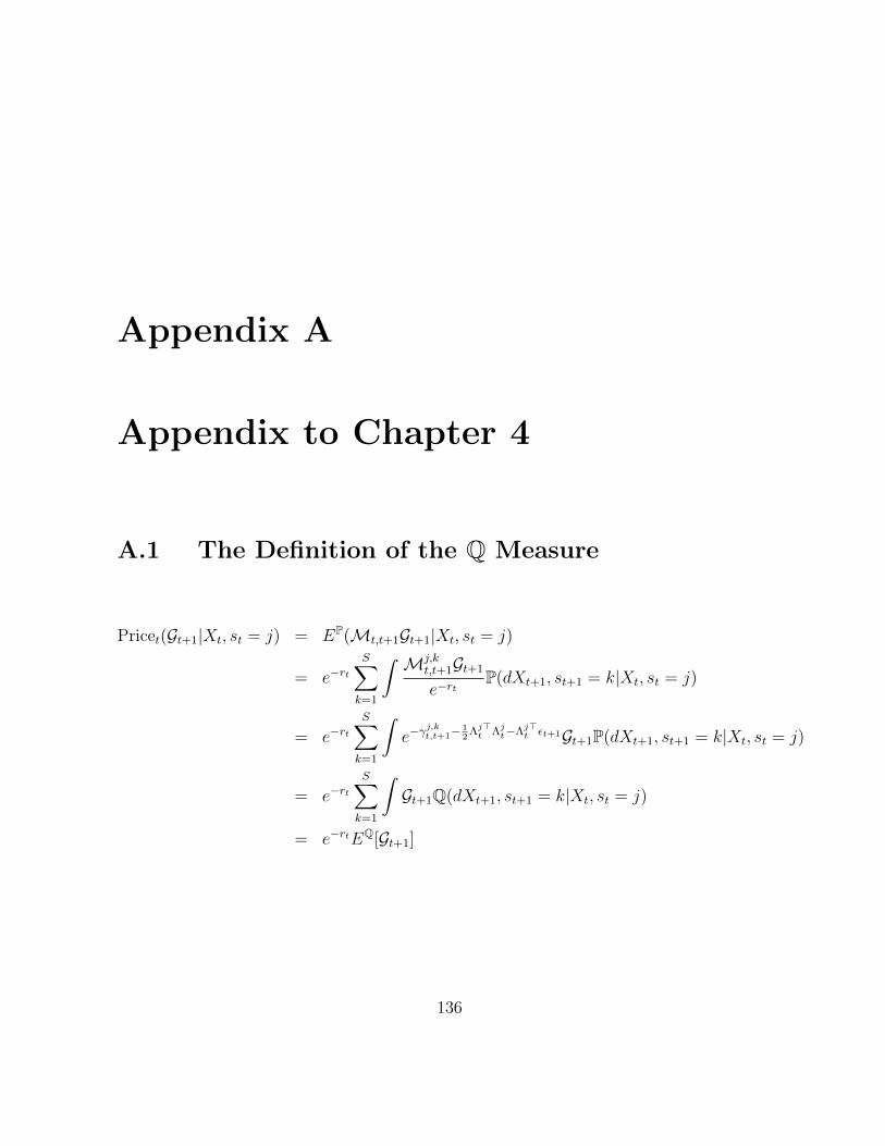
Appendix A
Appendix to Chapter 4
A.1 The Definition of the Q Measure
Pricet(Gt+1|Xt, st = j) = EP(Mt,t+1Gt+1|Xt, st = j)
= e−rtS∑k=1
∫ Mj,kt,t+1Gt+1
e−rtP(dXt+1, st+1 = k|Xt, st = j)
= e−rtS∑k=1
∫e−γ
j,kt,t+1−
12
Λj>t Λj
t−Λj>t εt+1Gt+1P(dXt+1, st+1 = k|Xt, st = j)
= e−rtS∑k=1
∫Gt+1Q(dXt+1, st+1 = k|Xt, st = j)
= e−rtEQ[Gt+1]
136

A.2 Xt in the Q Measure
Denote EPt,j[·] ≡ EP [·|Xt, st = j]. Before deriving the dynamic of Xt in measure Q, observe
that the no arbitrage price of a zero coupon bond that pays $1 at t+ 1 is:
e−rt = EPt,j [1 · Mt,t+1] = EP
t,j
[e−rt−γt,t+1− 1
2Λ>t Λt−Λ>t εt+1
],
which implies:
1 = EPt,j
[e−γt,t+1
]=
S∑k=1
πj,ke−γ(j,k)
The conditional moment generation function (MGF) of Xt+1 given st = j is
EQ[eu>Xt+1 |Xt, st = j
]= ertEP
[Mt,t+1e
u>Xt+1|Xt, st = j]
= EPt,j
[e−γt,t+1− 1
2Λ>t Λt−Λ>t εt+1 · eu>Xt+1
]= EP
t,j
[e−γt,t+1− 1
2Λ>t Λt−Λ>t εt+1 · eu>(α(st)+β(st)Xt)+u>Σ(st)εt+1
]= EP
t,j
[e−γt,t+1
]· EP
t,j
[e−
12
Λ>t Λt−Λ>t εt+1 · eu>(α(st)+β(st)Xt)+u>Σ(st)εt+1
]= EP
t,j
[e−
12
Λ>t Λt+u>(α(st)+β(st)Xt)+(u>Σ(st)−Λ>t )εt+1
]= e
− 12
Λ(j)>t Λ
(j)t +u>(α(j)+β(j)Xt)+
12
(u>Σ(j)−Λ
(j)>t
)(u>Σ(j)−Λ
(j)>t
)>
= eu>(α(j)+β(j)Xt−Σ(j)Λ
(j)t )+ 1
2u>Σ(j)Σ(j)>u
= eu>(α(j)−Λ(j)+β(j)Xt+
12u>ΣjΣj>u
= eu>(αj+βjXt)+
12u>ΣjΣj>u,
which implies that the behavior of Xt+1 is as follows:
Xt+1 = α(st) + β(st)Xt + Σ(st)εt+1
137

A.3 Futures Price Formula Derivation
Ft,n = EQ [Ft+1,n−1|Xt, st = j]
Fn (Xt, st) = EQ [Fn−1 (Xt+1, st+1) |Xt, st = j]
eA(j)n +B
(j)n Xt = EQ
[eA
(st+1)
n−1 +B(st+1)
n−1 Xt+1|Xt, st = j]
=S∑k=1
πjkEQ[eA
(k)n−1+B
(k)n−1Xt+1
]=
S∑k=1
πjkEQ[eA
(k)n−1+B
(k)n−1(α(j)+β(j)Xt+Σ(j)εt+1)
]=
S∑k=1
πjkeA
(k)n−1+B
(k)n−1(α(j)+β(j)Xt)EQ
[eB
(k)n−1Σ(j)εt+1
]=
S∑k=1
πjk · eA(k)n−1+B
(k)n−1(α(j)+β(j)Xt)+ 1
2B
(k)n−1Σ(j)Σ(j)>B
(k)>n−1
A(j)n +B(j)
n Xt = log
(S∑k=1
πjk · eA(k)n−1+B
(k)n−1(α(j)+β(j)Xt)+ 1
2B
(k)n−1Σ(j)Σ(j)>B
(k)>n−1
)
since β(1) = β(2) for both B&S-RS and G&S models and setting B(n)(1) = B(n)(2) = B(n),
one gets:
A(j)n +BnXt = Bn−1βXt + Log
(S∑k=1
πjk · eA(k)n−1+Bn−1α(j)+ 1
2Bn−1Σ(j)Σ(j)>B>n−1
)
138

Wich implies:
A(j)n = Log
(S∑k=1
πjk · eA(k)n−1
)+Bn−1α
(j) +1
2Bn−1Σ(j)Σ(j)>B>n−1
Bn = Bn−1β.
A.4 Hamilton (1994) Filtration Procedure
Step 1 Calculate Pr[st−1 = i, st = j|Jt−1]as following:
Pr[st−1 = i, st = j|Jt−1] =Pr[st = j|st−1] ·S∑h=1
Pr[st−2 = h, st−1 = i|Jt−1]
=π(i,j)t−1,t ·
S∑h=1
Pr[st−2 = h, st−1 = i|Jt−1],
where π(i,j)t−1,t is the transitional probability and can be taken rom the transitional
matrix.
Step 2 Calculate the joint density function of yt and (st−1, st) as following:
f(yt, st−1 = i, st = j|Jt) = f(yt|st−1 = i, st = j, Jt) · Pr[st−1 = i, st = j|Jt−1]
where
f(yt|st−1 = i, st = j, Jt) = (2π)−N/2|H(i,j)t |−1/2exp(−1
2η
(i,j)>t|t−1 H
(i,j)t η
(i,j)t|t−1).
139
Step 3 Calculate :
Pr[st−1 = i, st = j|Jt] =f(yt, st−1 = i, st = j|Jt−1)
f(yt|Jt−1)(A.1)
where
f(yt|Jt−1) =S∑j=1
S∑i=1
f(yt, st−1 = i, st = j|Jt−1).
140