Essays in International Economics - Academic Commons

Essays in International Economics

Jing Zhou

Submitted in partial fulfillment of therequirements for the degree of

Doctor of Philosophyin the Graduate School of Arts and Sciences

COLUMBIA UNIVERSITY

2018

ABSTRACT

Essays in International Economics

Jing Zhou

The three chapters of my dissertation study the macroeconomics and firm dynam-

ics under financial frictions and institutional frictions. They contain both theoretical

and empirical analysis with a special emphasis on the scope of open economy and

the implications on policy.

Chapter 1 presents a theoretical framework to study the debt portfolio choice and

optimal capital control policy in an open economy with financial frictions. I extend the

model of international borrowing with collateral constraint to allow for multiple debt

maturities. As in the single-maturity version of the model, the equilibrium exhibits

overborrowing because, due to a pecuniary externality, private agents undervalue the

cost of financial liabilities that demand repayment in future constrained states. I show

that in the multiple-maturity model overborrowing in short-term debt is especially

severe because the repayment of short-term liabilities is larger than that of long-term

liabilities in future constrained states, resulting in greater cost undervaluation of short-

term financial obligations. To counteract these inefficiencies, the model justifies a set

of maturity-dependent capital controls. The model predicts a tightening of capital

controls tilted toward short maturities during financial crises. When calibrated to

Argentine data, the model reproduces the observed dynamics of debt portfolios,

and the short-term targeting of capital controls during crises. The optimal capital-

control policy reduces the frequency of crises by half and generates sizable welfare

improvements.

Motivated by the policy implications of Chapter 1, the second chapter of my dis-

sertation presents an empirical study of how capital control policies are implemented

in financial crises. I construct a novel measure of capital control stringency and

establish three stylized facts about the capital control changes around financial crisis.

First, capital control policies do not show significant changes until the onset of finan-

cial crisis (procyclicality). Second, not only outflow controls but also inflow controls

are strengthened upon the arrival of financial crisis (dual tightening). Third, inflow

controls show strong emphasis towards curbing short-term flows, while outflow

controls are generally enhanced with respect to a wide range of flows regardless of

their maturities (short-term maturity targeting). These patterns are robust to countries

with different economy stances, external indebtedness, exchange-rate regimes and

capital control levels.

Besides the financial frictions, the institutional frictions also play important roles

in the external finance. Therefore, the third chapter of my dissertation examines

the role of public governance quality in determining the composition of a country’s

external liabilities and the capital structure of firms. In this joint work with Shang-Jin

Wei, we first build a model with firm heterogeneity to show that better institutional

quality tends to promote a higher share of foreign direct investment and equity

investment in total foreign liabilities, and a higher share of long-term debt within the

debt/loan category. Similar prediction holds for the capital structure of firms. We

then conduct extensive empirical investigation by exploring both firm level data and

country level data and find supportive evidence for these predictions.

Contents

List of Figures iii

List of Tables v

1 Financial Crises, Debt Maturity, and Capital Controls 1

1.1 Introduction . . . . . . . . . . . . . . . . . . . . . . . . . . . . . . . . . . 1

1.2 Related Literature . . . . . . . . . . . . . . . . . . . . . . . . . . . . . . . 5

1.3 Stylized Facts on External Borrowing in Financial Crises . . . . . . . . . 7

1.4 The Model . . . . . . . . . . . . . . . . . . . . . . . . . . . . . . . . . . . 9

1.5 Quantitative Analysis . . . . . . . . . . . . . . . . . . . . . . . . . . . . . 20

1.6 Conclusion . . . . . . . . . . . . . . . . . . . . . . . . . . . . . . . . . . . 48

2 Capital Controls in Financial Crises: An Empirical Analysis 51

2.1 Introduction . . . . . . . . . . . . . . . . . . . . . . . . . . . . . . . . . . 52

2.2 The Data . . . . . . . . . . . . . . . . . . . . . . . . . . . . . . . . . . . . 57

2.3 Economy Fluctuations in Financial Crises . . . . . . . . . . . . . . . . . 62

2.4 The Cyclicality of Capital Control in Financial Crises . . . . . . . . . . . 63

2.5 Capital Control On Different Types of Transactions in Financial Crises 68

2.6 The Maturity Targeting of Capital Controls . . . . . . . . . . . . . . . . 80

2.7 Maturity-dependent Reserve Requirements . . . . . . . . . . . . . . . . 82

2.8 Conclusion . . . . . . . . . . . . . . . . . . . . . . . . . . . . . . . . . . . 84

i

3 Quality of Public Governance and the Capital Structure

of Nations and Firms (with Shang-Jin Wei) 87

3.1 Introduction . . . . . . . . . . . . . . . . . . . . . . . . . . . . . . . . . . 88

3.2 The Model . . . . . . . . . . . . . . . . . . . . . . . . . . . . . . . . . . . 92

3.3 The Data . . . . . . . . . . . . . . . . . . . . . . . . . . . . . . . . . . . . 103

3.4 Capital Structure of External Financing . . . . . . . . . . . . . . . . . . . 105

3.5 Structure of Domestic Financing and Institutional Quality . . . . . . . . 108

3.6 Conclusion . . . . . . . . . . . . . . . . . . . . . . . . . . . . . . . . . . . 125

Bibliography 127

Appendix to Chapter 1 134

Procedure for Constructing Index of Changes in Capital Control . . . . . . . 135

Proof of Proposition 1 . . . . . . . . . . . . . . . . . . . . . . . . . . . . . . . . 136

Proof of Proposition 2 . . . . . . . . . . . . . . . . . . . . . . . . . . . . . . . . 137

Ruling Out Multiple Equilibria . . . . . . . . . . . . . . . . . . . . . . . . . . 137


Categorization of Transaction and Flows . . . . . . . . . . . . . . . . . . . . . 142

The Procedure of Constructing Measures of Capital Control from "Changes"

Section . . . . . . . . . . . . . . . . . . . . . . . . . . . . . . . . . . . . . 143


Proofs . . . . . . . . . . . . . . . . . . . . . . . . . . . . . . . . . . . . . . . . . 148

Internal Financing and External Financing . . . . . . . . . . . . . . . . . . . . 149

Going Beyond Listed Firms . . . . . . . . . . . . . . . . . . . . . . . . . . . . 149

FDI and Equity Portfolio Investment . . . . . . . . . . . . . . . . . . . . . . . 150

Nonlinear Implications of the Model . . . . . . . . . . . . . . . . . . . . . . . 153

ii

List of Figures

1.1 External Financing in Financial Crises . . . . . . . . . . . . . . . . . . . . . 9

1.2 Term Premium: Calibration vs. Data . . . . . . . . . . . . . . . . . . . . . . 22

1.3 Term Premium: Calibration vs. Data . . . . . . . . . . . . . . . . . . . . . . 24

1.4 Ergodic Distribution of Total Debt: Friction versus Frictionless . . . . . . . 25

1.5 Insurance Benefit and Borrowing Cost of Long-term Debt Accumulation . 28

1.6 Ergodic Distribution of Maturity: Friction versus Frictionless . . . . . . . . 30

1.7 Dynamics in Financial Crises . . . . . . . . . . . . . . . . . . . . . . . . . . 32

1.8 Optimal Capital Control in Financial Crisis Window . . . . . . . . . . . . . 35

1.9 Cyclicality of Optimal Capital Control . . . . . . . . . . . . . . . . . . . . . 36

1.10 Comparison Between Short- and Long-term Capital Controls . . . . . . . . 39

1.11 Optimal Long-term Capital Control Without Term Premium . . . . . . . . 41

1.12 Ergodic Distribution of Total Debt and Maturity . . . . . . . . . . . . . . . 44

1.13 Welfare Gains from Optimal Capital Controls . . . . . . . . . . . . . . . . . 45

2.1 Economy Fluctuations in Financial Crisis . . . . . . . . . . . . . . . . . . . 63

2.2 Capital Control Changes in Financial Crisis . . . . . . . . . . . . . . . . . . 67

2.3 Correlation Between Inflow and Outflow Controls Changes . . . . . . . . 68

2.4 Average Number of Capital Control Changes by Types of Transaction . . . 70

2.5 Capital Control Changes by Income Level . . . . . . . . . . . . . . . . . . . 72

2.6 Capital Control Changes by External Indebtedness . . . . . . . . . . . . . . 73

2.7 Capital Control Changes by Exchange Rate Regime . . . . . . . . . . . . . 74

iii

2.8 Capital Control Changes by Capital Control Level . . . . . . . . . . . . . . 76

2.9 Maturity Target of Capital Control Changes . . . . . . . . . . . . . . . . . . 81

2.10 Reserve Requirement on Foreign Currency Deposit . . . . . . . . . . . . . 83

3.1 Capital Structure: High Institutional Quality vs. Low Institutional Quality 102

3.2 Capital Structure and Institutional Quality . . . . . . . . . . . . . . . . . . 102

3.3 Capital Structure of External Financing and Institutional Quality . . . . . . 106

3.4 Capital Structure and Institutional Quality (Worldscope) . . . . . . . . . . 115

3.5 Density of Institutional Quality Long-Difference . . . . . . . . . . . . . . . 123

3.6 Capital Structure of Domestic Financing and Institutional Quality . . . . . 124

A1 External Borrowing . . . . . . . . . . . . . . . . . . . . . . . . . . . . . . . . 138

A2 Share of Short-term External Debt . . . . . . . . . . . . . . . . . . . . . . . . 138

A3 Dynamics and Optimal Capital Controls in Boom-Bust Periods . . . . . . . 139

A4 Dynamics and Optimal Capital Controls in Crises Periods . . . . . . . . . 140

C1 Changes in Capital Structure Distribution To Institutional Quality Im-

provement . . . . . . . . . . . . . . . . . . . . . . . . . . . . . . . . . . . . . 154

C2 Quantile Regression Estimates . . . . . . . . . . . . . . . . . . . . . . . . . . 154

iv

List of Tables

1.1 Parameter Values . . . . . . . . . . . . . . . . . . . . . . . . . . . . . . . . . 23

1.2 Statistics: Model and Data . . . . . . . . . . . . . . . . . . . . . . . . . . . . 23

1.3 Crisis Severity Comparison Between Competitive Equilibrium and Ram-

sey Equilibrium . . . . . . . . . . . . . . . . . . . . . . . . . . . . . . . . . . 33

1.4 Welfare Effect of Constrained Optimal Capital Controls . . . . . . . . . . . 48

2.1 Summary Statistics . . . . . . . . . . . . . . . . . . . . . . . . . . . . . . . . 59

2.2 Comparison Among Capital Control Measures . . . . . . . . . . . . . . . . 60

2.3 Capital Control Changes: Sudden Stop Versus Peak and Recovery . . . . . 78

2.4 Capital Control Changes by Flow Type: Sudden Stop Versus Peak and

Recovery . . . . . . . . . . . . . . . . . . . . . . . . . . . . . . . . . . . . . . 78

3.1 External Capital Structure and Institutional Quality . . . . . . . . . . . . . 109

3.2 External Capital Structure and Institutional Quality - Balanced Sample . . 110

3.3 External Liability and Institutional Quality - Control for Foreign Reserves 111

3.4 External Capital Structure and Institutional Quality - Logit . . . . . . . . . 112

3.5 Institutional Quality and Capital Structure . . . . . . . . . . . . . . . . . . 117

3.6 Institutional Quality and Corporate Bond Maturity . . . . . . . . . . . . . 118

3.7 Equity and Different Measures of Institutional Quality . . . . . . . . . . . . 119

3.8 Long-term Debt and Different Measures of Institutional Quality . . . . . . 120

3.9 External/Internal Financing and Institutional Quality . . . . . . . . . . . . 122

v

3.10 Top Ten and Bottom Ten Countries in the Change of Institutional Quality

(2003 vs. 2015) . . . . . . . . . . . . . . . . . . . . . . . . . . . . . . . . . . . 123

3.11 Long Difference . . . . . . . . . . . . . . . . . . . . . . . . . . . . . . . . . . 125

C1 Cross-correlation table . . . . . . . . . . . . . . . . . . . . . . . . . . . . . . 145

C2 Summary Statistics for External Financing . . . . . . . . . . . . . . . . . . . 145

C3 Summary Statistics of Worldscope firms . . . . . . . . . . . . . . . . . . . . 146

C4 Country Composition of Worldscope Sample . . . . . . . . . . . . . . . . . 147

C5 Summary Statistics of Compustat firms . . . . . . . . . . . . . . . . . . . . 148

C6 Summary Statistics of Amadeus Firms . . . . . . . . . . . . . . . . . . . . . 150

C7 Country Composition of Amadeus Sample . . . . . . . . . . . . . . . . . . 151

C8 Capital Structure of Domestic Financing and Institutional Quality . . . . . 152

C9 FDI, Equity Portfolio Investment, and Institutional Quality . . . . . . . . . 153

vi

Acknowledgements

I owe special thanks to my dedicated sponsors, Martín Uribe and Shang-Jin Wei.

They have been my role models and inspirations in research, and I would never

have gone this far without their kind guidance and generous help. My research

interest in international economics begins from Professor Uribe’s field class. I am

deeply indebted to his advice on my works, patience with my trials and failures,

and encouragement for my self-doubts. Professor Wei is the professor that I first

approached to at Columbia, and I have been privileged to work with him on projects.

His diversified research ideas have broadened my horizon, and I am especially

grateful to him for lightening my way in my darkest moments.

I also benefited enormously from my committee members Stephanie Schmitt-

Grohé, Andres Drenik, and Jesse Schreger. I began to discuss with them about my

research in the late years, but I wish I had more time to work with them. They have

provided extremely helpful comments in improving my papers, and they have been

incredibly generous with time given their busy schedules.

I am very lucky to have the opportunities to exchange ideas with other faculties

at Columbia and researchers from conferences and internships. I would like to thank

Juan Hatchondo, Emi Nakamura, B. Ravikumar, Juan Sánchez, and Jón Steinsson for

their valuable advice. I would also like to thank Ricardo Reis for his advice for my

research in the early years of graduate school.

I am grateful to have the best coauthors and friends for their help throughout the

journey. I would like to thank JaeBin Ahn, Carlos Carvalho, Gee Hee Hong, Yang Jiao,

vii

Nandita Krishnaswamy, Sun Kyoung Lee, Rui Mano, Danna Thomas, Lin Tian, Zhe

Wang, and Peichu Xie. I would also like to thank my high school teacher Luqiang

Wang for his support for the first year Ph.D.

For the most, I am forever indebted to my parents for being there for me. Without

their unconditional support, nothing would ever have been possible.

viii

To my parents

ix

Chapter 1

Financial Crises, Debt Maturity, and Capital Controls

1.1 Introduction

Episodes of financial crisis are often associated with two patterns that have been

extensively documented: large movements in capital flows1 and drastic shift to

shorter-maturity flows.2 The first pattern, namely the surges and stops in capital

flows, has resulted in a strong push to revamp capital control as an essential form of

regulation.3 Regarding the second pattern about short-term flows, the emerging view

emphasizes that short-term liabilities render an economy particularly vulnerable

to rollover crises or self-fulfilling liquidity crises and that long-term debt should

be favored.4 However, if the risk of short-term debt is correctly perceived and

incorporated in optimal decisions, then the large proportion of short-term debt

means that the gains from increased short-term debt today exceed the expected

costs of financial distress in the future. Therefore, the questions remain: is short-

term liability accumulation inefficient ex ante? Under what conditions does private

agents’ optimization lead to inefficient debt portfolio choice compared with the social

optimal? What should be the design of optimal regulating policies to counteract the

1For the main stylized facts see for instance, Gourinchas et al. (2001), Mendoza and Terrones (2008),Rogoff and Reinhart (2009), Broner et al. (2013a).

2See Brunnermeier (2009), Arellano and Ramanarayanan (2012), Broner et al. (2013b).3See Ostry et al. (2010), Rey (2015), Korinek (2017), Jeanne and Korinek (2010), and Bianchi (2011a),

among many others.4See, for example, Cole and Kehoe (2000), Alfaro and Kanczuk (2009), Jeanne (2009).

1

inefficiencies?

This paper aims to address these questions from the theoretical perspective. I

argue that with financial frictions, (i) the debt portfolio in the competitive economy

is inefficient in terms of overborrowing and excess short-term debt issuing, and (ii)

these inefficiencies can be eliminated through the adoption of a set of state-contingent

and maturity-dependent capital inflow controls. I develop a small open economy

model where external borrowing is available in multiple maturities yet subject to

collateral constraint and risk-averse international creditors. I use the model to analyze

the mechanism inducing inefficiency, to derive and verify optimal capital control

policy, and to evaluate welfare improvement generated by the optimal policy.

To inspect the underlying mechanism, I build a model that embeds multiple debt

maturities and risk-averse international creditors in a standard collateral constraint

model à la Korinek (2017) and Bianchi (2011a). As in the single-maturity version

of the model, the equilibrium exhibits overborrowing because, due to a pecuniary

externality, private agents undervalue the cost of financial liabilities that demands re-

payment in future constrained states. The key insight of the multiple-maturity model

is that overborrowing in short-term debt is especially severe because the repayment

of short-term liabilities is larger than that of long-term liabilities in future constrained

states. Therefore, pecuniary externality leads to two sorts of inefficiency in private

agents’ debt portfolio decision: (i) overborrowing regardless of debt maturity, which

is in line with the literature such as Korinek (2017) and Bianchi (2011a), and more

importantly (ii) excess short-term debt issuing, which is new to the literature.

How does pecuniary externality play a role in shaping debt portfolio? In the

model, optimal debt portfolio is determined by two sets of trade-offs: inter-temporal

trade-off and the intra-temporal trade-off. On the inter-temporal perspective, private

agents trade off between the current benefit of borrowing and the associated future

2

repayment cost. However, the repayment cost is undervalued in the future states

where collateral constraint binds. This undervaluation arises because by taking

collateral price as given, private agents evaluate the cost of repayment as the utility

loss from the direct one-to-one consumption decrease. However, they neglect that,

with collateral constraint binding, debt repayment triggers financial amplification:

consumption decrease lowers collateral price and value, limits borrowing capacity,

and further constrains consumption. This contractionary spiral magnifies the future

repayment cost, yet it is not internalized by private agents.

On the intra-temporal perspective, the key difference between the short- and

long-term debt is the amount of required repayment. Given current short-term

borrowing rate, its demanded repayment is independent with next period’s states.

On the contrary, the price of long-term debt decreases in response to interest rate

hike, which is often associated with future crisis states, exhibiting insurance against

adverse shocks. Therefore, long-term debt’s repayment cost is effectively low in future

collateral constrained states. Given the same undervaluation per unit repayment, the

low repayment level of long-term debt leads to milder cost undervaluation than that

of the short-term, resulted in excess short-term debt issuing.

In order to counteract these inefficiencies stemming from pecuniary external-

ity, I prove that the social optimal debt portfolio can be decentralized by a set of

state-contingent and maturity-dependent capital controls, and I derive a close-form

solution for the capital control taxes. To shed further light on the design of capital con-

trol policy, I analyze two aspects: cyclicality and maturity-dependence. I first focus on

the cyclicality, which is equivalent to the cyclicality of the level of undervaluation in

future repayment cost. The magnitude of this undervaluation is determined by two

factors: the probability of future crisis and the magnitude of financial amplification

effect. Due to the persistence of shocks, crisis in current period indicates a high

3

probability of future crisis, and the low consumption in crisis leads to a large financial

amplification effect. Therefore, pecuniary externality in crisis exceeds that in normal

time, which directly yields capital controls tightening for both short- and long-term

inflows in crisis.

Another important feature of the optimal capital control policy is the short-term

inflow targeting, which hinges on the relative magnitude of repayment cost underval-

uation between short-term debt and long-term debt. Essentially, this level of relative

undervaluation can be decomposed into the product of (i) the undervaluation of

future cost per unit of repayment (ii) the magnitude of repayment difference between

short-term and long-term debt. The former peaks in crisis, following the same logic

as in the analysis of cyclicality. The latter is the new ingredient, which is governed

by the term premium. As is supported by the data, term premium surges in crisis.

Therefore, compared with the long-term debt, the repayment cost of short-term debt

is more undervalued, and most severely undervalued in crisis, which requires tighter

short-term inflow control in general, and especially tighter in crisis.

When calibrated to Argentine data, the model can reproduce external borrowing

collapse, maturity shrinking, and the behavior of the key aggregate variables in crisis.

The model also successfully generates the overborrowing and excess short-term debt

of the competitive economy compared with the social optimum. In terms of the

optimal capital control policies, the model derives a set of capital inflow taxes that

hike in crisis and target short-term inflow.

The quantitative analysis also shows significant welfare improvements by the

optimal capital controls. Crisis frequency drops by half, and the severity of crisis is

substantially alleviated, for instance, the magnitude of tradable consumption decrease

reduces by 17%, the real exchange rate depreciation is 24% smaller. On average, the

improvement in life-time utility is equivalent to 0.59% consumption increase. The

4

welfare analysis also demonstrates the importance of distinguishing maturity in

capital controls because the maturity-independent capital controls can only achieve

half of the welfare improvement generated by the maturity-dependent counterpart.

Comparing the welfare effects by short-term inflow control and that of the long-term,

the analysis shows that the welfare improvement from exclusive long-term inflow

control produces only 10% of that from exclusive short-term inflow control. This

result indicates that if policymakers are constrained in policy tools then short-term

inflow control should be set as the priority.

The rest of the paper is organized as follows. Section 1.2 discusses the related

literature. Section 1.3 presents the empirical facts about external borrowing in fi-

nancial crisis episodes. Section 1.4 builds a dynamic small open economy model

including external borrowing under collateral constraint with different maturities

and risk-averse international creditors. Section 1.5 discusses the main mechanism

relating debt portfolio choice and optimal capital control policy, and it also presents

the model calibration, the quantitative results, and the optimal policy evaluation.

Section 1.6 concludes and discusses possible future extensions.

1.2 Related Literature

This paper contributes towards four main strands of literature. First, this paper

adds to the growing quantitative studies of pecuniary externality due to collateral

constraints and the remedies. Seminal papers of Korinek (2017), Jeanne and Korinek

(2010), and Bianchi (2011a), show the presence of market price in collateral constraint

generates pecuniary externality which calls for capital controls. Recent papers have

extended the model in different directions, for instance, production economy as

Benigno et al. (2013), alternative policy instruments as Benigno et al. (2016a), time

consistent policy as Bianchi and Mendoza (2013) and Devereux et al. (2015), cyclicality

5

of capital control as Schmitt-Grohé and Uribe (2017). However, the existing works

have focused exclusively on the interaction between pecuniary externality and short-

term debt.5 This paper builds on these studies by introducing endogenous debt

maturity structure and showing that pecuniary externality leads to inefficiencies in

not only quantity of debt but also maturity structure of debt. These dual effects

of pecuniary externality give rise an extra layer in optimal policy design that both

state-contingency and maturity-dependence are necessary to restore social optimal

equilibrium.

Second, this paper is related to the literature on the optimal maturity structure

of debt. There has been a growing strand of works studying the maturity structure

of sovereign debt, including Hatchondo and Martinez (2009), Arellano and Rama-

narayanan (2012), Chatterjee and Eyigungor (2012), Broner et al. (2013b), and Aguiar

and Amador (2013), rationalizing the relationship between maturity structure, bor-

rowing cost, and default decision. Different from their focus on the financial friction

resulted from no repayment commitment, I study another form of financial friction as

the limit of borrowing capacity based on the pledged collateral. Despite the difference

in modeling financial friction, this paper shares a similar logic with the defaultable

debt literature in the trade-off underlying optimal maturity choice, such as the in-

surance benefit of long-term debt and the cost benefit of short-term debt. Moreover,

I focus on the external borrowing from the private sector and the ineffcient in the

competitive equilibrium compared with social optimum, and this new angle provides

the room for studying policy interventions. Within the defaultable debt literature,

there have been works discussing the disavantage of short-term debt in terms of

rollover risk and self-fulling liquidity risk, for instance, Cole and Kehoe (2000), Alfaro

5One important exception is Korinek (2017), which discusses the general principle of capital controltax with respect to different types of capital flows. However, it does not endogenize the maturitystructure of external borrowing and its interaction with capital control policy.

6

and Kanczuk (2009), and Jeanne (2009). However, this paper differs from them in

analyzing the ex ante efficiency of debt portfolio choice and provide a close form

illustration of the optimal policy. There is also a large literature in corporate finance

on the optimal maturity structure of debt. Recent developments include short-term

debt and rollover risk, including Brunnermeier and Yogo (2009), He and Xiong (2012),

Farhi and Tirole (2012), and Brunnermeier and Oehmke (2013). Instead of these static

models, this paper examines the optimal maturity structure and its cyclical features

in a dynamic framework where financial crises endogenously rise.

Third, the theoretical implication of capital control policies during financial crisis

episodes is related to the recent literature on capital control policy implementation

in practice. Fernández et al. (2015a) provide a comprehensive analysis showing

that capital control is acyclical. Focusing on the sovereign default crises, Na et al.

(2014a) find that capital controls are significantly tightened. This paper contributes

the literature by analyzing the dynamics of capital control policies in a new set of

important economy episodes: financial crises. Similar to Na et al. (2014a), I also find

capital controls are more restricted in the bust of crisis episodes. Combining with the

existing evidence, this implies there might be non-linear relationship between capital

control policies and business cycle in a way that the policy is likely to respond to only

severe shocks in economy. As a result, capital control policy seems not responding to

business cycle in general but only to significant economy fluctuations.

1.3 Stylized Facts on External Borrowing in Financial

Crises

This section examines the patterns of private external borrowing in financial crisis

episodes. Specifically, this analysis focuses on the amount of private external borrow-

7

ing, the maturity choice, and the capital inflow regulations around financial crisis

episodes. The external borrowing data shows that the amount of private external

borrowing collapses during financial crises and the private debt portfolio significantly

tilts towards short-term borrowing, consistent with the literature.

1.3.1 External Borrowing and Maturity Structure

Utilizing the International Debt Statistics dataset (1970 - 2016) from the World Bank,

I calculate external borrowing as the change in external debt stock in private sector

and measure maturity structure by the share of private sector short-term debt in total

private sector debt. For the interest of financial crises, I focus on the 139 financial

crisis windows (114 countries, 1970 -2011) identified by (Laeven and Valencia, 2013)

and evaluate the changes in the quantity and the maturity composition of private

external borrowing across crisis windows.

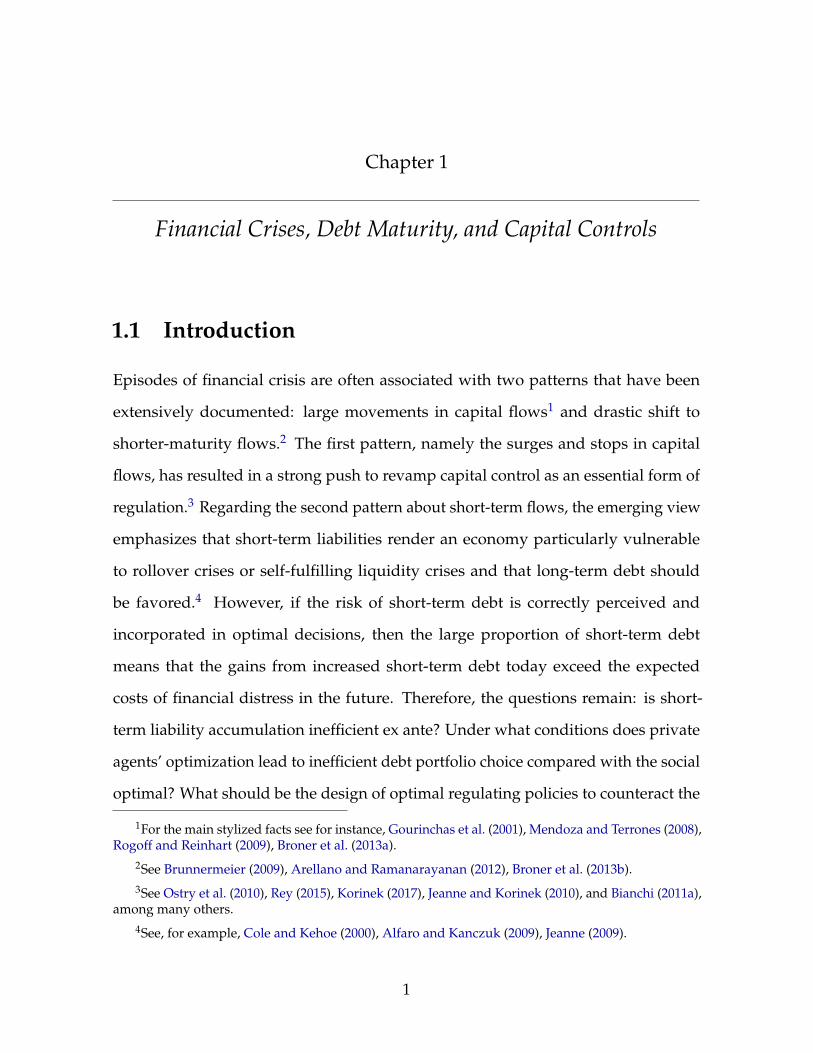
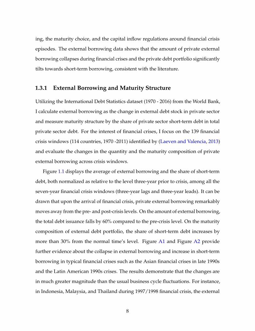
Figure 1.1 displays the average of external borrowing and the share of short-term

debt, both normalized as relative to the level three-year prior to crisis, among all the

seven-year financial crisis windows (three-year lags and three-year leads). It can be

drawn that upon the arrival of financial crisis, private external borrowing remarkably

moves away from the pre- and post-crisis levels. On the amount of external borrowing,

the total debt issuance falls by 60% compared to the pre-crisis level. On the maturity

composition of external debt portfolio, the share of short-term debt increases by

more than 30% from the normal time’s level. Figure A1 and Figure A2 provide

further evidence about the collapse in external borrowing and increase in short-term

borrowing in typical financial crises such as the Asian financial crises in late 1990s

and the Latin American 1990s crises. The results demonstrate that the changes are

in much greater magnitude than the usual business cycle fluctuations. For instance,

in Indonesia, Malaysia, and Thailand during 1997/1998 financial crisis, the external

8

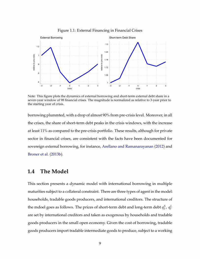
Figure 1.1: External Financing in Financial Crises

.4

.6

.8

1

1.2

rela

tive

to p

re-c

risis

-3 -2 -1 0 1 2 3crisis

External Borrowing

1

1.06

1.12

1.18

1.24

1.3

rela

tive

to p

re-c

risis

-3 -2 -1 0 1 2 3crisis

Short-term Debt Share

Note: This figure plots the dynamics of external borrowing and short-term external debt share in aseven-year window of 98 financial crises. The magnitude is normalized as relative to 3-year prior tothe starting year of crisis.

borrowing plummted, with a drop of almost 90% from pre-crisis level. Moreover, in all

the crises, the share of short-term debt peaks in the crisis windows, with the increase

at least 11% as compared to the pre-crisis portfolio. These results, although for private

sector in financial crises, are consistent with the facts have been documented for

sovereign external borrowing, for instance, Arellano and Ramanarayanan (2012) and

Broner et al. (2013b).

1.4 The Model

This section presents a dynamic model with international borrowing in multiple

maturities subject to a collateral constraint. There are three types of agent in the model:

households, tradable goods producers, and international creditors. The structure of

the mdoel goes as follows. The prices of short-term debt and long-term debt qSt , qL

t

are set by international creditors and taken as exogenous by households and tradable

goods producers in the small open economy. Given the cost of borrowing, tradable

goods producers import tradable intermediate goods to produce, subject to a working

9

capital constraint. Given stochastic streams of nontradable goods income (yN), debt

prices (qSt , qL

t ), and the rebated profit from tradable goods producers, representative

households issue short- and long-term debt under collateral constraint to finance the

optimal consumption allocation. Section 1.4.A illustrates the optimization problem of

each agent, Section 1.4.B explains the first order conditions and defines competitive

equilibrium, Section 1.4.C introduces Ramsey equilibrium and derives the optimal

capital control policy.

1.4.1 Environment

Household – The representative household in the economy receives utility from

consumption with preference given by

E

∞

∑t=0

βtu(ct) (1.1)

where β ∈ (0, 1) is the discount factor and u(·) is assumed to have the constant-

relative-risk-aversion (CRRA) form. The total consumption c is constituted by trad-

able goods consumption cT and nontradable goods consumption cN with Armington-

type CES aggregator

ct =[α(cT

t )1−1/ξ + (1− α)(cN

t )1−1/ξ

] 11−1/ξ

where ξ denotes the elasticity of substitution between tradable and nontradable goods

and (1− α) ∈ (0, 1) is the home bias.

In every period t, households have two sources of income. The first is an exoge-

nous nontradable endowment yNt , and the second is the profit πt from the tradable

goods production. Besides domestic income, households also have access to the

global financial market by issuing short- and long-term debt. The external borrow-

ings in both maturities are in real term, and it is denominated by tradable goods.

Short-term debt is in the form of one-period discount bond. For one unit of short-term

10

bond issued, borrowers receive qSt unit of tradable goods and international creditors

demand one unit of tradable goods repayment in the next period. Long-term bond

is modeled as a perpetuity contract with deterministic infinite stream of coupons

that decay geometrically at an exogenous constant rate δ, following Hatchondo and

Martinez (2009) and Arellano and Ramanarayanan (2012). Specifically, one unit of

long-term bond yields qLt of tradable goods for the borrower upon issuance and

mandates δn−1 of tradable goods repayment for every future period t + n. Therefore,

the law of motion of long-term debt repayment can be represented by

dLt+1 = δdL

t + it

where dLt is the repayment for long-term debt in period t, and it is the amount of

newly-issued long-term bond in period t. As the bonds are non-defaultable and the

borrower is in a small scale compared with the global financial market, I assume

that qSt and qL

t are exogenous to the small open economy. With these specifications,

households’ inter-temporal budget constraint can be written as

cTt + ptcN

t + dSt + dL

t = πt + ptyNt + qS

t dSt+1 + qL

t (dLt+1 − δdL

t ) (1.2)

where pt denotes the relative price of nontradable goods in terms of tradable goods,

or equivalently, the real exchange rate.

Although households can finance consumption using international financial mar-

ket, the financing is subject to frictions. I assume that the international creditors

impose a collateral constraint on households as the total value of debt outstanding in

each period no larger than a fraction κ ∈ (0, 1) of their contemporaneous income.

qSt dS

t+1 + qLt dL

t+1 ≤ κ(πt + ptyNt ) (1.3)

This collateral constraint is in a similar vein as Bianchi (2011a) except for the inclusion

of long-term debt, and it can be viewed as “maintenance margin requirement” fol-

lowing Mendoza and Smith (2006). Essentially, it protects the creditors from default

11

by insuring that the face value of debt can be recovered by the market value of the

pledged collateral.6

The collateral constraint affects the dynamics of the small open economy in two

aspects. On one hand, it brings in financial frictions by limiting the amount external

borrowing and lowering welfare compared to the frictionless case. On the other hand,

it introduces pecuniary externality as households take the price of nontradable goods

as exogenous when allocating consumption and borrowing, yet they neglect that the

price is determined by their collective optimal consumption and borrowing choices.

This externality, as will be discussed in details later, differentiates the competitive

equilibrium from social planner’s Ramsey equilibrium, which justifies the importance

of external borrowing regulations.

Tradable Goods Producers – The tradable goods in household’s consumption bun-

dle is produced by the tradable sector using imported tradable goods ft using the

following technology:

yTt = Γ f γ

t , γ ∈ (0, 1), Γ > 0

I assume that while producing, the producer faces a working capital constraint

such that fraction η of the input factor payment must be paid in advance before

production or sale takes place, and the rest (1− η) can be paid after the production

and sale complete. In order to finance the working capital requirement, firms have

6Following Jeanne and Korinek (2010), the collateral constraint can be micro-founded in the sameway as the moral hazard problem. Assume that international creditors cannot coordinate to punishthe borrower by excluding him from borrowing in future periods. In the meantime, the borrower hasthe option to invest in a scam that allows him to remove his future endowment income from the reachof his current creditors. This would allow him to default on his debts next period without facing apenalty. However, the creditors can observe the scam in the current period and take the insider to courtbefore the scam is completed. If they do so, they can seize a fraction κ of the borrower’s collateral,where κ captures imperfect legal enforcement. The creditor can re-sell the collateral at the prevailingmarket price. This implies the participation condition for the creditor to lend to the borrower shouldtake the form of (1.3).

12

to borrow η ft in units of tradable goods (the working capital) at price qSt ,7, which

will incur interest rate cost ( 1qS

t− 1)η ft. Therefore, tradable goods producers’ profit

maximization problem can be stated in the following way:

maxft

πt = Γ f γt − ft − (

1qS

t− 1)η ft (1.4)

The tradable production sector with working capital constraint connects the econ-

omy’s income to the international financial market conditions, by doing so it provides

a micro-foundation for otherwise exogenously imposed dependence between y and

q.8

International Creditors – I assume risk-averse international creditors and their stochas-

tic discount factor takes the form of Ang and Piazzesi (2003).9

ln Mt,t+1 = −φ0 − φ1xt −12

ζ2t σ2

x − ζtεx,t+1

ζt = φζ0 + φ

ζ1 xt

xt+1 = φx0(1− φx

1) + φx1 xt + εx,t+1

where xt is the factor in determining international investor’s pricing kernel, ζt is

the time-varying market price of risk associated with the sources of uncertainty εx.

Examples of the shocks to international creditor’s stochastic discount factor could be

7Here the timing is that the loan is made at the beginning of each period and repaid at the end ofthe period, so the contemporaneous debt price is used, same as Mendoza (2010). However, Neumeyerand Perri (2005) Chang and Fernández (2013) use the last period interest rate.

8The link between borrower’s income and borrowing rate has been convincingly justified in thedefault literature as income affects the probability of default and hence the price of borrowing. How-ever, without default, it is less straightforward to associate the external borrowing rate to borrower’sincome other than the collateral constraint channel embedded in the model. Here I take workingcapital constraint framework, which is a workhorse model used in analyzing the business cycle ofemerging countries in response to external interest rate, for instance, Neumeyer and Perri (2005), Uribeand Yue (2006), etc. Alternative justification could be both borrower’s tradable income and lender’srisk appetite depend on world-wide income shock.

9This specification of the lender’s stochastic discount factor is a special case of the one-factor modelof the term structure, and it has been used in models of sovereign default, for instance, Arellano andRamanarayanan (2012), Bocola and Dovis (2016).

13

time preference change, world-wide demand shifter, or uncertainty shocks. Note that,

if λt is zero for all t, which means the price of risk is nil, then international creditors

are risk-neutral. To understand why international creditors are risk-averse even they

are able to receive repayments in any state, it is key to note that the effective value

of long-term debt repayment varies with states. For short-term debt, international

creditors will be repaid by one unit in each case next period, therefore, there is no risk.

However, the effective repayment for long-term debt is state-dependent, different

from short-term debt. Specifically, the effective repayment, which is equal to the

present value of all future repayments, is (1 + δqLt+1), which hinges on the future

state in period t + 1. In other words, the effective repayment will be different based

on different values of stochastic discount factor, and this connection between Mt,t+1

and (1 + δqLt+1) yields risk aversion. Essentially, international creditors’ stochastic

discount factor generates a time-varying term premium between short- and long-

term debt, and as will be shown in the next section, time-varying term premium is

critical in the model for interior optimal portfolio solution and the relative magnitude

between short- and long-term capital control taxes.

1.4.2 Competitive Equilibrium

To define the competitive equilibrium, I begin with the optimal condition for the

tradable goods producers’ static profit maximization problem. Producers choose the

amount of imported tradable goods to maximize profit according to (1.4), taking qSt

as given. The producer’s first order condition requires:

γΓ f γ−1t = 1 + (

1qS

t− 1)η

It further yields the optimal level of profit

πt = Γ(1− γ)[1 + ( 1

qSt− 1)η

γΓ

] γγ−1

(1.5)

14

The households’ problem is to choose {cTt , cN

t , dSt+1, dL

t+1} to maximize the present

discounted value of life-time utility in (1.1) subject to budget constraint (1.2) and

collateral constraint (1.3), given tradable goods production profit (1.5), exogenous

nontradable endowment yNt , and bond prices qS

t , qLt . The corresponding first order

conditions are:

u′Tt = λt (1.6)

pt =1− α

α

( cTt

cNt

)1/ξ(1.7)

λtqSt − µtqS

t = βEtλt+1 (1.8)

λtqLt − µtqL

t = βEt

[λt+1

(1 + δqL

t+1)]

(1.9)

µt[κ(πt + ptyN

t)− qS

t dSt+1 − qL

t dLt+1]= 0, with µt ≥ 0 (1.10)

dSt+1 + dL

t+1 ≤ κ(πt + ptyN

t)

(1.11)

where βtλt is the Lagrangian multiplier for budget constraint and βtµt is the La-

grangian multiplier associated with collateral constraint. Equation (1.6) requires the

marginal utility of tradable consumption equal to the shadow value of current income.

Equation (1.7) determines the relative price of tradable goods by marginal rate of sub-

stitution between tradable goods and nontradable goods consumption. Equation (1.8)

and (1.9) are the Euler equations associated with short-term debt and long-term debt.

Because of different debt prices and repayment schedule, the short-term and long-

term Euler equations differ from each other in both the contemporaneous benefit of

one unit of debt and the expected cost of the associated future repayment. Compared

to the scenario with financial frictions, collateral constraint lays a wedge between

the present value of consumption and the expected value of future repayment for

both short-term debt and long-term debt. Specifically, as shown in Equation (1.8)

and (1.9), when the financial crisis occurs, meaning collateral constraint binds, the

shadow price of collateral constraint penalizes extra consumption through borrowing

15

in both maturities. Finally, equation (1.10) and (1.11) state the slackness conditions of

collateral constraint.

Because nontradable goods can only be consumed domestically and that there is

no heterogeneity among households, market clear conditions are:

cNt = yN

t (1.12)

cTt + dS

t + dLt = πt + qS

t dSt+1 + qL

t (dLt+1 − δdL

t ) (1.13)

Definition 1. (Competitive Equilibrium) The competitive equilibrium is defined as a set of

processes {cTt , cN

t , dSt+1, dL

t+1, pt, πt, λt, µt}∞t=0 satisfying optimal conditions (1.5) to (1.13),

given exogenous processes {yNt , qS

t , qLt }∞

t=0 and initial debt levels dS0 , dL

0 .

1.4.3 Ramsey Equilibrium and Optimal Capital Controls

One important feature of the competitive equilibrium is that agents take the market

prices as given, particularly in choosing debt portfolio, households take the collateral

price (nontradable goods price) as given. Unlike the household in the competitive

equilibrium, social planner recognizes how the aggregate variables, especially non-

tradable goods price, is determined in equilibrium and takes it into account when

determining the optimal external financial decisions. Given this difference, it is impor-

tant to compare private agents’ decision and social planner’s choice, and this section

explains social planner’s optimization problem and its connection to the competitive

equilibrium.

I assume a benevolent social planner who maximizes the life-time utility of house-

holds. The planner can choose debt portfolio for households and let the consumption

portfolio and market price to be determined in the competitive way. Therefore, the

Ramsey equilibrium from social planner’s optimization problem can be defined as

follows.

16

Definition 2. (Ramsey Equilibrium) The Ramsey equilibrium is defined as a set of processes

{cTt , cN

t , dSt+1, dL

t+1, pt, πt}∞t=0 maximizing the present discounted utility (1.1) subject to

collateral constraint (1.3), pricing rule (1.7), and market clear conditions (1.12) and (1.13),

given exogenous processes {yNt , qS

t , qLt }∞

t=0 and initial debt levels dS0 , dL

0 .

Ramsey equilibrium and competitive equilibrium share a number of optimal

conditions, while they significantly differ from each other in choosing debt portfolio.

To shed further light on the difference, it would be useful to analyze the Euler

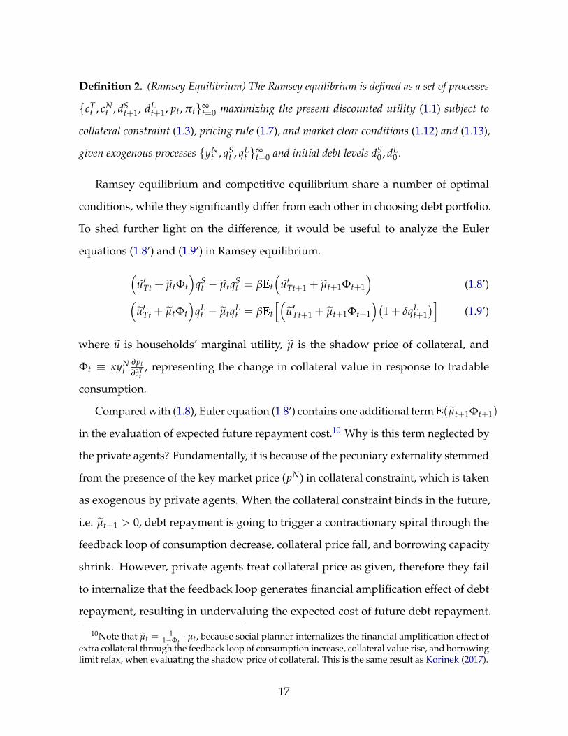
equations (1.8’) and (1.9’) in Ramsey equilibrium.

(u′Tt + µtΦt

)qS

t − µtqSt = βEt

(u′Tt+1 + µt+1Φt+1

)(1.8’)(

u′Tt + µtΦt

)qL

t − µtqLt = βEt

[(u′Tt+1 + µt+1Φt+1

)(1 + δqL

t+1)]

(1.9’)

where u is households’ marginal utility, µ is the shadow price of collateral, and

Φt ≡ κyNt

∂ pt∂cT

t, representing the change in collateral value in response to tradable

consumption.

Compared with (1.8), Euler equation (1.8’) contains one additional termE(µt+1Φt+1)

in the evaluation of expected future repayment cost.10 Why is this term neglected by

the private agents? Fundamentally, it is because of the pecuniary externality stemmed

from the presence of the key market price (pN) in collateral constraint, which is taken

as exogenous by private agents. When the collateral constraint binds in the future,

i.e. µt+1 > 0, debt repayment is going to trigger a contractionary spiral through the

feedback loop of consumption decrease, collateral price fall, and borrowing capacity

shrink. However, private agents treat collateral price as given, therefore they fail

to internalize that the feedback loop generates financial amplification effect of debt

repayment, resulting in undervaluing the expected cost of future debt repayment.

10Note that µt =1

1−Φt· µt, because social planner internalizes the financial amplification effect of

extra collateral through the feedback loop of consumption increase, collateral value rise, and borrowinglimit relax, when evaluating the shadow price of collateral. This is the same result as Korinek (2017).

17

The magnitude of pecuniary externality is determined by the probability of future col-

lateral constraint binding (µt+1) and the financial amplification effect when collateral

constraint binds (Φt+1).

Similar to short-term debt’s Euler equation, the long-term debt’s counterpart (1.9’)

also includes an extra term in the expect future cost of debt issuing, Etµt+1Φt+1(1 +

δqLt+1). However, different from short-term debt which requires one unit of repay-

ment, one unit of long-term debt demands(1 + δqL

t+1)

units of “effective” repayment

at t + 1.11 Therefore, the associated pecuniary externality is(1 + δqL

t+1)

times as of

short-term debt in each future collateral constrained state.

Given the difference between competitive equilibrium and Ramsey equilibrium,

a natural question would be whether the Ramsey equilibrium allocation can be

supported as a regulated competitive equilibrium or not. To analyze the optimal

policy intervention, I follow the literature (i.e. Korinek (2017), Bianchi (2011a), etc.)

and assume that social planner has two policy tools: tax on short-term borrowing and

tax on long-term borrowing, and that the total tax revenue is rebated to household in

a lump-sum way. Specifically, households maximize the present discounted value

of life-time utility given capital control taxes, and the optimization problem can be

formalized as follows.

Definition 3. (Competitive Equilibrium Under Regulation) The competitive equilibrium un-

der capital control policies is defined as a set of processes {cTt , cN

t , dSt+1, dL

t+1, pt, πt, λt, µt}∞t=0

satisfying optimal conditions (1.5) to (1.13), given exogenous processes {yNt , qS

t , qLt }∞

t=0,

initial debt levels dS0 , dL

0 , and capital control taxes {τSt , τL

t }∞t=0 maximizing the present dis-

11“Effective” repayment of long-term debt is the discounted present value of all the future paymentsof long-term debt. Alternatively, it could be viewed as the cost of retiring one unit of long-term debt.

18

counted utility (1.1) subject to collateral constraint (1.3) and budget constraint

cTt + ptcN

t + dSt + dL

t = πt + ptyNt + (1− τS

t )qSt dS

t+1 + (1− τLt )q

Lt (d

Lt+1 − δdL

t ) + Tt

(1.2’)

where Tt = τSt qS

t dSt+1 + τL

t qLt (d

Lt+1 − δdL

t ).

In order to decentralizing the Ramsey equilibrium, social planner chooses taxes

to maximize household’s present discounted utility while allowing debt portfolio

to be chosen by the private agents given the after-tax debt price, and that goods

market clear competitively under collateral constraint. Accordingly, the optimization

problem can be defined as follows.

Definition 4. (Ramsey Optimal Competitive Equilibrium) The Ramsey optimal competitive

equilibrium is defined as a set of processes {τSt , τL

t , cTt , cN

t , dSt+1, dL

t+1, pt, πt, λt, µt}∞t=0 maxi-

mizing the present discounted utility (1.1) subject to pricing rule (1.7), slackness conditions

(1.10) and (1.11), market clear conditions (1.12) and (1.13), and Euler equations under reg-

ulation (1.8”) and (1.9”), given exogenous processes {yNt , qS

t , qLt }∞

t=0 and initial debt levels

dS0 , dL

0 .

λtqSt (1− τS

t )− µtqSt = βEtλt+1 (1.8”)

λtqLt (1− τL

t )− µtqLt = βEt

[λt+1

(1 + δ(1− τL

t+1)qLt+1)]

(1.9”)

Proposition 1. (Optimal Capital Controls) The Ramsey optimal allocation can be decentral-

ized in a competitive equilibrium with taxes on short- and long-term debt satisfying

τSt = 1− β · Eλt+1

qSt λt

(1.14)

λtqLt (1− τL

t ) = βEt

[λt+1

(1 + δ(1− τL

t+1)qLt+1)]

(1.15)

where λ is the optimal shadow price of income in Ramsey equilibrium.

The optimal capital control policy (see proof in Appendix A) follows the same

logic as Schmitt-Grohé and Uribe (2017) that social planner can always choose tax

19

rates such that individual agents’ trade-off between contemporaneous benefit of

borrowing and the expected future cost of repayment coincides with that of social

planner. Essentially, since the future cost of repayment is undervalued by private

agents, capital control taxes on external borrowing are set to decrease the benefit of

borrowing to balance out the miscalculation of cost.

Summary of the Model – The model differs from a standard collateral constraint

model in small open economy from two aspects: first, instead of one short-term debt,

the model grants borrower the access to long-term debt, which introduces maturity

choice in equilibrium; second, international creditor is risk-averse, which generates

term premium in external borrowing. The economy is driven by stocks in interna-

tional creditor’s stochastic discount factor, whose dynamics will affect the borrowing

cost faced by the small open economy, and consequently, total debt position, maturity

structure, and consumption portfolio. The inefficiency in private agents’ debt matu-

rity structure due to pecuniary externality gives room for policy intervention, and the

state-contingent and maturity-dependent optimal policy is able to correct pecuniary

externality and restore social optimum.

1.5 Quantitative Analysis

This section presents the quantitative analysis of the model. Section 1.5.A describes

the parameterization and compares the key statistics from the competitive economy

simulation to the data. Section 1.5.B discusses the trade-offs that determines the

debt portfolio choice. Section 1.5.C analyzes the cyclicality of optimal capital control

polices. Section 1.5.D inspects the difference between short- and long-term capital

controls. Section 1.5.E studies the optimal debt portfolio in competitive equilibrium

and Ramsey equilibrium. Section 1.5.F evaluates the welfare effect of optimal capital

20

controls.

1.5.1 Parameterization and Key Statistics

I calibrate the model to Argentine data (1983 – 2001) with the time unit as one year.

Table 1.1 shows the values of parameters.12 Following Bianchi (2011a), the risk

aversion level is set at 2, the elasticity of substitution between tradable goods and

nontradable goods is set at 0.83, the weight on tradables in CES aggregator is set at

31%, and the collateral constraint tightness κ is set at 0.32. The time discount factor

β is set to be 0.86 to keep β/qS at the same value as Bianchi (2011a). The decaying

rate of long-term bond is set at 0.90 to match the average duration of private sector

external borrowing in the data.

The international creditors’ stochastic discount factor (SDF) and tradable sector

production are new to the literature, and they are calibrated in the following way. For

the SDF, first, I choose the factor xt as the Moody’s Seasoned Baa Corporate Bond

Spread as the proxy for global risk, and estimate the AR(1) process to obtain φx0 , φx

1

and σ2x . Global risk has been shown as an important factor in driving the variation

in interest rate and key macro variables in emerging economy. For instance, Akıncı

(2013) finds that global financial risk shocks explain about 20% of movements both

in the country spread and in the aggregate activity in emerging economies. To shed

further light on the relationship between global risk and the Argentine interest rates,

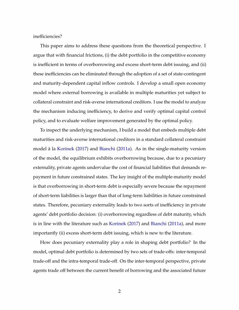
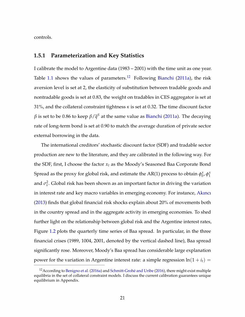
Figure 1.2 plots the quarterly time series of Baa spread. In particular, in the three

financial crises (1989, 1004, 2001, denoted by the vertical dashed line), Baa spread

significantly rose. Moreover, Moody’s Baa spread has considerable large explanation

power for the variation in Argentine interest rate: a simple regression ln(1 + it) =

12According to Benigno et al. (2016a) and Schmitt-Grohé and Uribe (2016), there might exist multipleequilibria in the set of collateral constraint models. I discuss the current calibration guarantees uniqueequilibrium in Appendix.

21

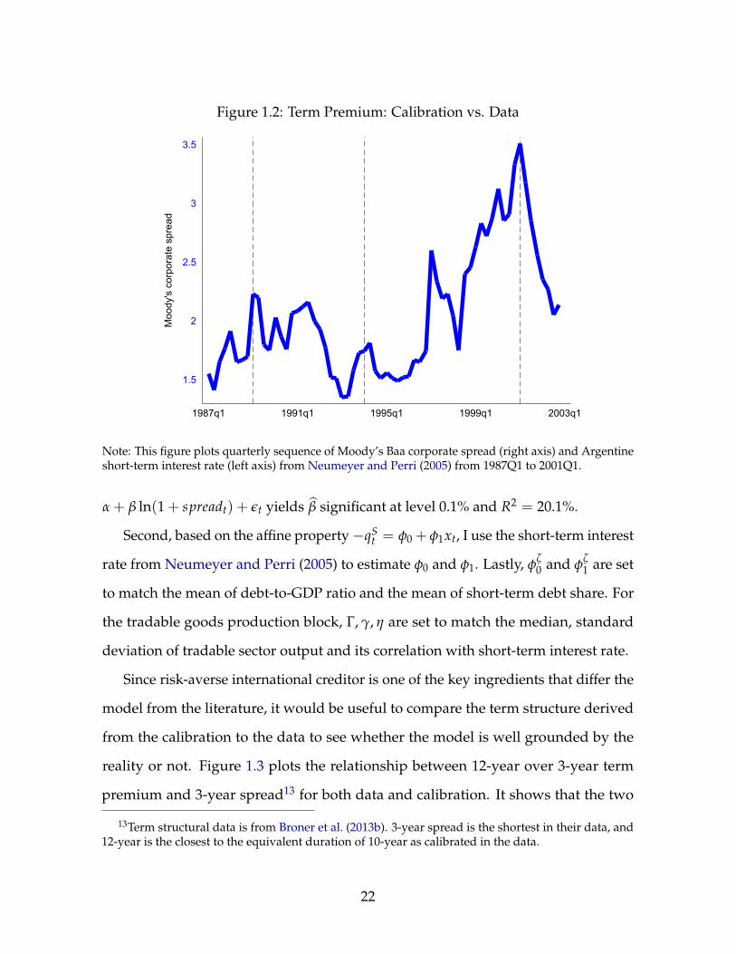
Figure 1.2: Term Premium: Calibration vs. Data

1.5

2

2.5

3

3.5

Moo

dy's

cor

pora

te s

prea

d

1987q1 1991q1 1995q1 1999q1 2003q1

Note: This figure plots quarterly sequence of Moody’s Baa corporate spread (right axis) and Argentineshort-term interest rate (left axis) from Neumeyer and Perri (2005) from 1987Q1 to 2001Q1.

α + β ln(1 + spreadt) + εt yields β significant at level 0.1% and R2 = 20.1%.

Second, based on the affine property−qSt = φ0 + φ1xt, I use the short-term interest

rate from Neumeyer and Perri (2005) to estimate φ0 and φ1. Lastly, φζ0 and φ

ζ1 are set

to match the mean of debt-to-GDP ratio and the mean of short-term debt share. For

the tradable goods production block, Γ, γ, η are set to match the median, standard

deviation of tradable sector output and its correlation with short-term interest rate.

Since risk-averse international creditor is one of the key ingredients that differ the

model from the literature, it would be useful to compare the term structure derived

from the calibration to the data to see whether the model is well grounded by the

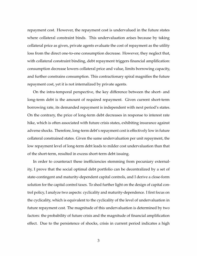
reality or not. Figure 1.3 plots the relationship between 12-year over 3-year term

premium and 3-year spread13 for both data and calibration. It shows that the two

13Term structural data is from Broner et al. (2013b). 3-year spread is the shortest in their data, and12-year is the closest to the equivalent duration of 10-year as calibrated in the data.

22

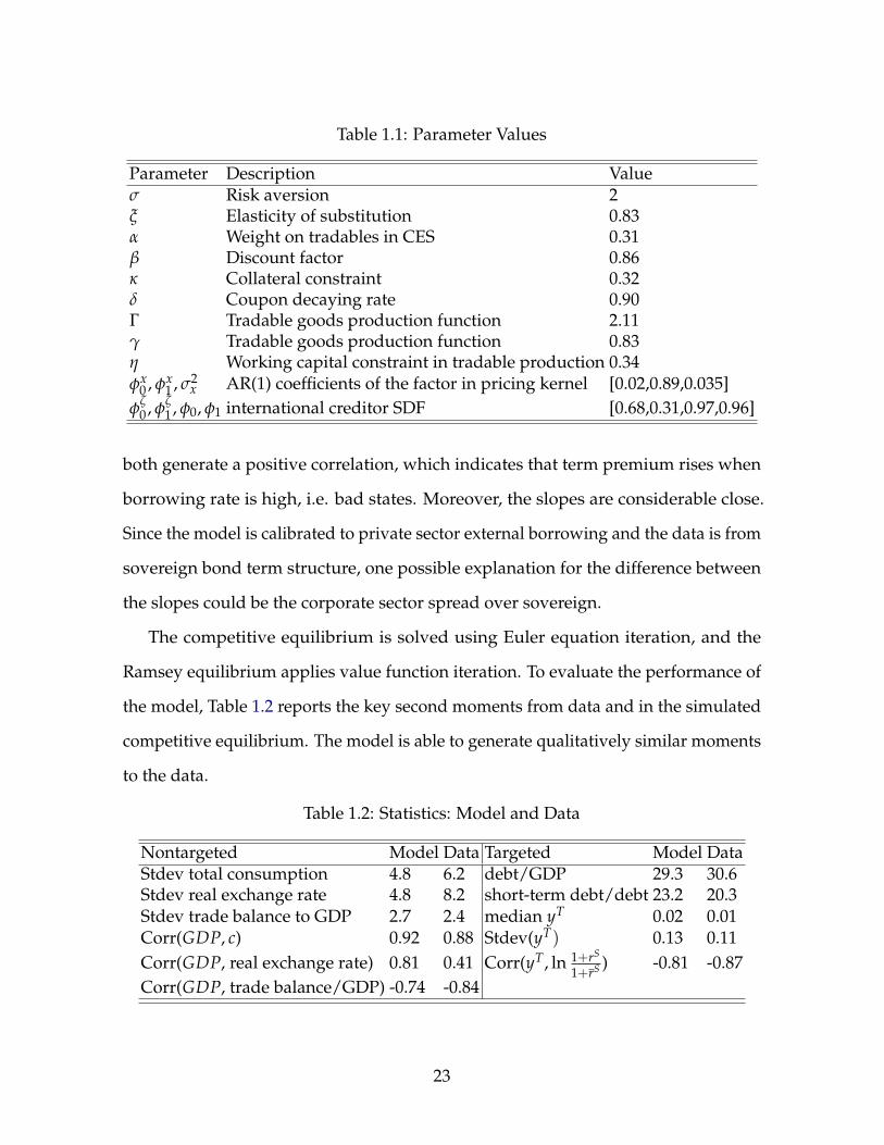
Table 1.1: Parameter Values

Parameter Description Valueσ Risk aversion 2ξ Elasticity of substitution 0.83α Weight on tradables in CES 0.31β Discount factor 0.86κ Collateral constraint 0.32δ Coupon decaying rate 0.90Γ Tradable goods production function 2.11γ Tradable goods production function 0.83η Working capital constraint in tradable production 0.34φx

0 , φx1 , σ2

x AR(1) coefficients of the factor in pricing kernel [0.02,0.89,0.035]φ

ζ0 , φ

ζ1 , φ0, φ1 international creditor SDF [0.68,0.31,0.97,0.96]

both generate a positive correlation, which indicates that term premium rises when

borrowing rate is high, i.e. bad states. Moreover, the slopes are considerable close.

Since the model is calibrated to private sector external borrowing and the data is from

sovereign bond term structure, one possible explanation for the difference between

the slopes could be the corporate sector spread over sovereign.

The competitive equilibrium is solved using Euler equation iteration, and the

Ramsey equilibrium applies value function iteration. To evaluate the performance of

the model, Table 1.2 reports the key second moments from data and in the simulated

competitive equilibrium. The model is able to generate qualitatively similar moments

to the data.

Table 1.2: Statistics: Model and Data

Nontargeted Model Data Targeted Model DataStdev total consumption 4.8 6.2 debt/GDP 29.3 30.6Stdev real exchange rate 4.8 8.2 short-term debt/debt 23.2 20.3Stdev trade balance to GDP 2.7 2.4 median yT 0.02 0.01Corr(GDP, c) 0.92 0.88 Stdev(yT) 0.13 0.11Corr(GDP, real exchange rate) 0.81 0.41 Corr(yT, ln 1+rS

1+rS ) -0.81 -0.87Corr(GDP, trade balance/GDP) -0.74 -0.84

23

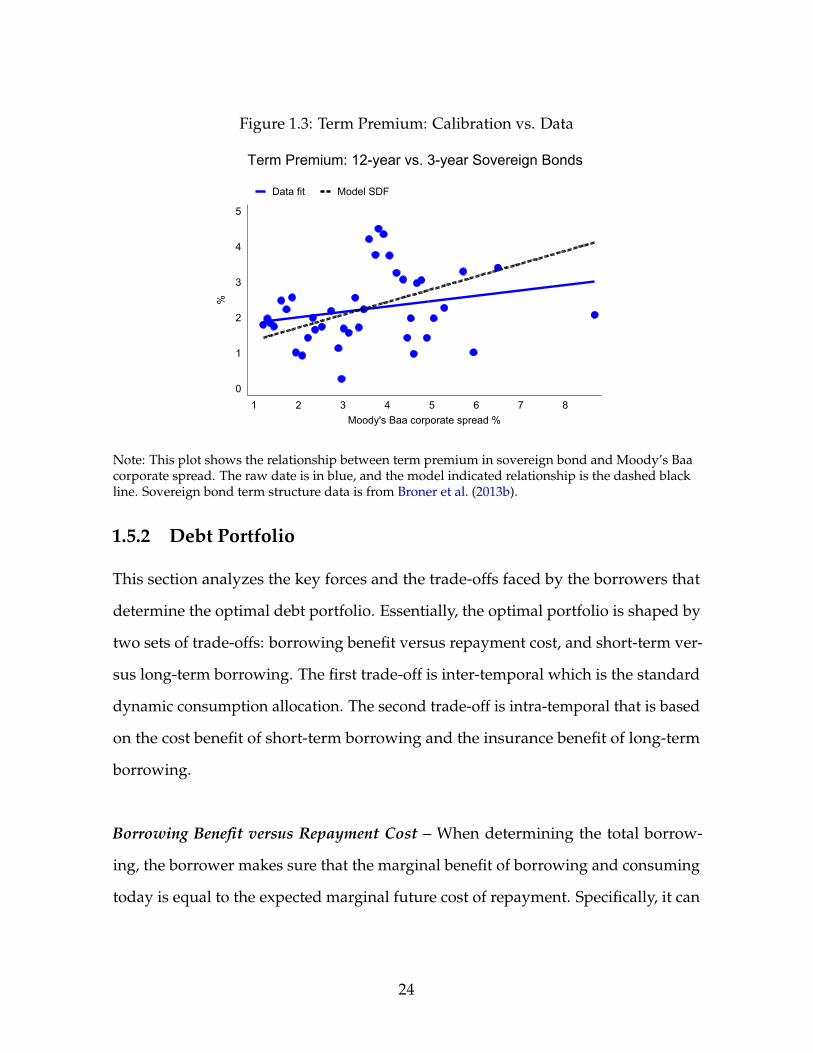
Figure 1.3: Term Premium: Calibration vs. Data

0

1

2

3

4

5%

1 2 3 4 5 6 7 8Moody's Baa corporate spread %

Data fit Model SDF

Term Premium: 12-year vs. 3-year Sovereign Bonds

Note: This plot shows the relationship between term premium in sovereign bond and Moody’s Baacorporate spread. The raw date is in blue, and the model indicated relationship is the dashed blackline. Sovereign bond term structure data is from Broner et al. (2013b).

1.5.2 Debt Portfolio

This section analyzes the key forces and the trade-offs faced by the borrowers that

determine the optimal debt portfolio. Essentially, the optimal portfolio is shaped by

two sets of trade-offs: borrowing benefit versus repayment cost, and short-term ver-

sus long-term borrowing. The first trade-off is inter-temporal which is the standard

dynamic consumption allocation. The second trade-off is intra-temporal that is based

on the cost benefit of short-term borrowing and the insurance benefit of long-term

borrowing.

Borrowing Benefit versus Repayment Cost – When determining the total borrow-

ing, the borrower makes sure that the marginal benefit of borrowing and consuming

today is equal to the expected marginal future cost of repayment. Specifically, it can

24

be represented by the Euler equation of consumption.

u′TtqSt − µtqS

t = βEtu′Tt+1

where µt is the Lagrangian multiplier of collateral constraint. Different from the

frictionless framework, the presence of collateral constraint punishes extra borrowing

if total borrowing already reaches the limit, and this wedge decreases the marginal

utility of borrowing ceteris paribus. As a result, private agents borrow less than if there

is no friction in borrowing. In other words, private agents realize that the desired

future borrowing might be unavailable due to collateral constraint, therefore they

accumulate precautionary saving to cope with the constrained borrowing capacity

in future bad states. Taken together, collateral constraint generates underborrowing

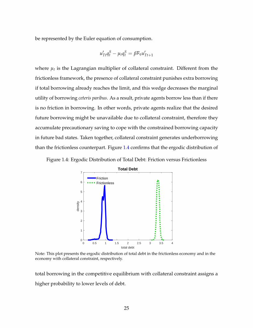
than the frictionless counterpart. Figure 1.4 confirms that the ergodic distribution of

Figure 1.4: Ergodic Distribution of Total Debt: Friction versus Frictionless

0 0.5 1 1.5 2 2.5 3 3.5 4

total debt

0

1

2

3

4

5

6

7

dens

ity

Total Debt

FrictionFrictionless

Note: This plot presents the ergodic distribution of total debt in the frictionless economy and in theeconomy with collateral constraint, respectively.

total borrowing in the competitive equilibrium with collateral constraint assigns a

higher probability to lower levels of debt.

25

Insurance Benefit versus Cost Benefit – When determining the maturity structure of

debt, private agents make sure that, given the total amount of debt, the subjective

discounted expected future repayment cost is the same no matter borrowing short-

term debt or long-term debt. To analyze the benefit and cost of deviating from the

optimal maturity structure by swapping short- and long-term debt, I compare all the

portfolios that yields the optimal consumption level (i.e. keeping total debt position

unchanged) in the current period.14 As the debt price is exogenous, these portfolios

maintain a constant ratio between the quantities of debt equal to the relative price of

debt. If presented in the (dSt+1, dL

t+1) quadrant, essentially, these portfolios constitute

a straight line.

qSt dS

t+1 + dLt dL

t+1 = yTt − cT

t − dSt − (1 + δqL

t+1)dLt

To evaluate these portfolios, since they yield the same debt and consumption in the

current period, it would be sufficient to compare their present discounted cost of

future repayments. To facilitate the comparison, I restate the borrower’s optimization

problem in the following recursive way.

V(dSt , dL

t , St) = maxcT

t ,dSt+1,dL

t+1

u(ct) + βEtV(dSt+1, dL

t+1, St+1)

s.t. cTt + dS

t + dLt = πt + qS

t dSt+1 + qL

t (dLt+1 − δdL

t )

qSt dS

t+1 + qLt dL

t+1 ≤ κ(πt + ptyNt )

πt = Γ(1− γ)[1 + ( 1

qSt− 1)η

γΓ

] γγ−1

where St represents the current exogenous states {qSt , qL

t , yNt }.

Consider the change in the present discounted value of future utility for a portfolio

that deviates from the optimal maturity structure with replacing short-term debt with

14This analysis has been used in Aguiar and Amador (2013) and Bianchi et al. (2012) to illustratematurity choice in defautable debt.

26

long-term debt. The overall change stems from two sources: the increase in dLt+1 and

the decrease in dSt+1. Applying envelope theorem, the change in households’ life-time

utility takes the form as following

d EtV(dSt+1, dL

t+1, St+1)

d dLt+1

∣∣∣∣∣cT

t

= Et(u′Tt+1 ·qL

t

qSt)− Et

[u′Tt+1(1 + δqL

t+1)]

The first term on the right-hand side represents the utility gain associated with the

decrease in short-term debt repayment and the second term is the utility loss due to

the increase in long-term debt repayment. The key difference between the two terms

is that the increase in long-term debt repayment (1 + δqLt+1) depends on future states

while the decrease in short-term debt repayment is pre-determined in period t, and

this difference leads to the insurance benefit of the long-term and the cost benefit of

the short-term, respectively.

To gain more insights in the trade-off between insurance and cost, I analyze these

two terms in turns. First, long-term debt provides insurance benefit, and the insurance

is grounded by the negative correlation between borrower’s marginal utility and the

repayment cost of long-term debt. Specifically, in future bad states, borrowing rate

increases, which aggravates the situation as private agents face a high borrowing cost

(low q), and consumption is low, leading to high marginal utility as private agents

are in great needs of consumption. In the meantime, However, the long-term debt

repayment, which effectively is equal to (1 + δqLt+1), decreases in future bad states.15

Therefore, although the high borrowing cost makes it difficult for the borrower to

obtain external financial resource, it reduces the repayment of long-term debt at the

same time. In other words, long-term debt helps to alleviate the adverse future states

by mandating low repayment, which provides insurance for the borrowers.

Second, as the counterforce against long-term debt’s insurance benefit, the low

15Effective repayment of long-term debt is the discounted value of all the future repayments, andequivalently, it is also the cost of retiring the existing long-term debt with the new market debt price.

27

average borrowing cost of short-term debt favors short-term liability accumulation.

Keeping everything else unchanged, consider an extreme case that a negative shock

in the current period and the spread between short- and long-term debt spikes, as a

result, long-term debt price converges to the short-term. In this scenario, it would be

overwhelmingly costly to issue long-term debt as it provides the same funds as the

short-term in the current period while demands more repayment in the future.

Figure 1.5: Insurance Benefit and Borrowing Cost of Long-term Debt Accumulation

0 2 4 6 8 10 12

Moody's Baa corporate bond spread (next period), %

-0.1

-0.05

0

0.05

0.1

0.15

0.2net benefit

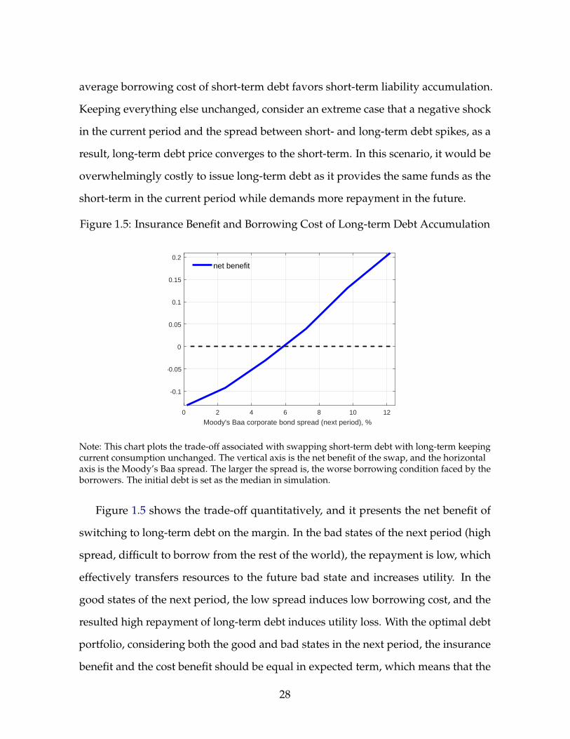
Note: This chart plots the trade-off associated with swapping short-term debt with long-term keepingcurrent consumption unchanged. The vertical axis is the net benefit of the swap, and the horizontalaxis is the Moody’s Baa spread. The larger the spread is, the worse borrowing condition faced by theborrowers. The initial debt is set as the median in simulation.

Figure 1.5 shows the trade-off quantitatively, and it presents the net benefit of

switching to long-term debt on the margin. In the bad states of the next period (high

spread, difficult to borrow from the rest of the world), the repayment is low, which

effectively transfers resources to the future bad state and increases utility. In the

good states of the next period, the low spread induces low borrowing cost, and the

resulted high repayment of long-term debt induces utility loss. With the optimal debt

portfolio, considering both the good and bad states in the next period, the insurance

benefit and the cost benefit should be equal in expected term, which means that the

28

weighted average of the values along the solid line is zero.

Having inspected the debt portfolio choice, one natural question is: what is the

role of collateral constraint in shaping the maturity structure? It can be observed that

with or without collateral constraint, the optimal intra-temporal condition remains

the same. Therefore, collateral constraint does not directly influence the insurance

versus cost trade-off. However, collateral constraint still affects maturity structure,

and its impact is indirectly through affecting the total debt position. The reason is that

keeping current utility constant requires total debt staying the same, which means no

matter how the composition of debt changes it will not invoke changes in collateral

constraint. As a result, this intra-temporal trade-off works in the same way as in the

portfolio choice without financial friction. However, as illustrated before, collateral

constraint plays a role in the inter-temporal trade-off and generates precautionary

saving and under-borrowing compared with frictionless case. Given that maturity

composition of debt depends on how much debt is taken in total, hence, maturity

changes along with overall debt position. Taken together, collateral constraint directly

alters aggregate amount of debt, as a side effect, maturity structure also changes.

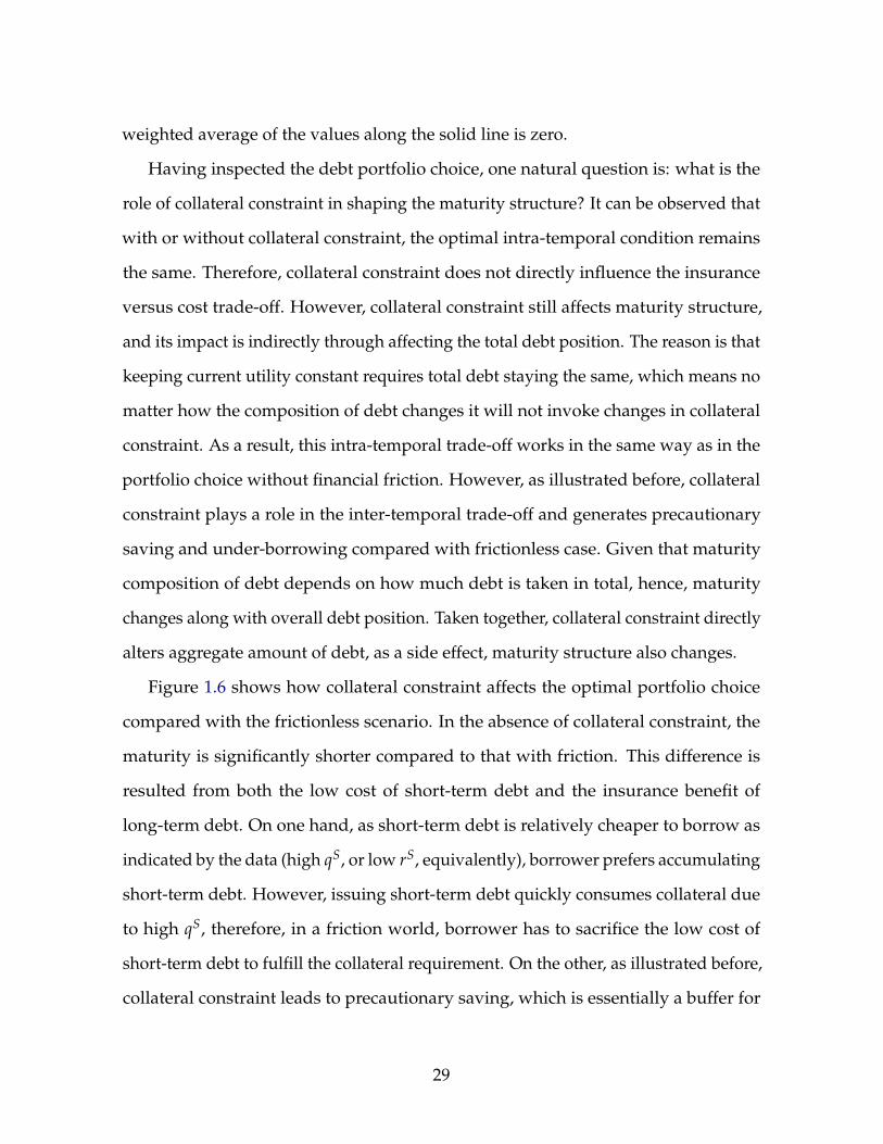
Figure 1.6 shows how collateral constraint affects the optimal portfolio choice

compared with the frictionless scenario. In the absence of collateral constraint, the

maturity is significantly shorter compared to that with friction. This difference is

resulted from both the low cost of short-term debt and the insurance benefit of

long-term debt. On one hand, as short-term debt is relatively cheaper to borrow as

indicated by the data (high qS, or low rS, equivalently), borrower prefers accumulating

short-term debt. However, issuing short-term debt quickly consumes collateral due

to high qS, therefore, in a friction world, borrower has to sacrifice the low cost of

short-term debt to fulfill the collateral requirement. On the other, as illustrated before,

collateral constraint leads to precautionary saving, which is essentially a buffer for

29

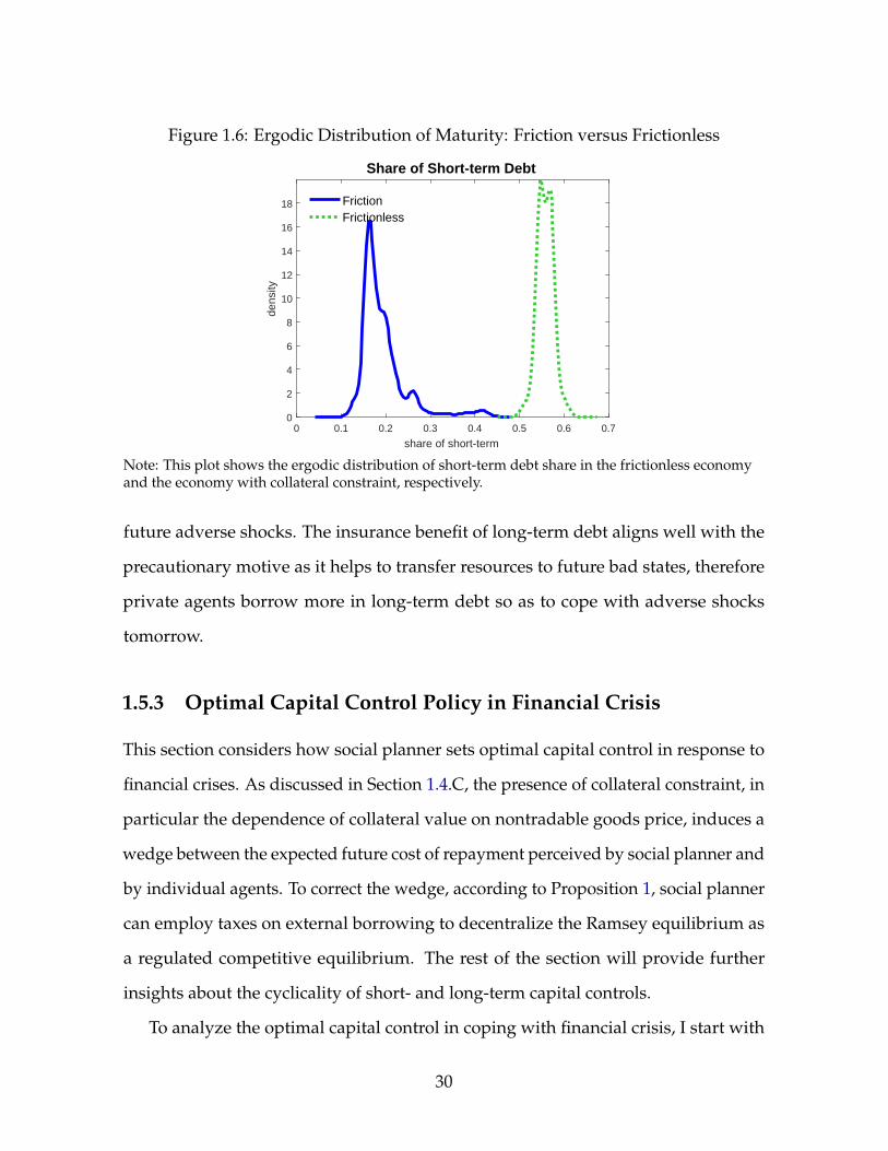
Figure 1.6: Ergodic Distribution of Maturity: Friction versus Frictionless

0 0.1 0.2 0.3 0.4 0.5 0.6 0.7

share of short-term

0

2

4

6

8

10

12

14

16

18

dens

ity

Share of Short-term Debt

FrictionFrictionless

Note: This plot shows the ergodic distribution of short-term debt share in the frictionless economyand the economy with collateral constraint, respectively.

future adverse shocks. The insurance benefit of long-term debt aligns well with the

precautionary motive as it helps to transfer resources to future bad states, therefore

private agents borrow more in long-term debt so as to cope with adverse shocks

tomorrow.

1.5.3 Optimal Capital Control Policy in Financial Crisis

This section considers how social planner sets optimal capital control in response to

financial crises. As discussed in Section 1.4.C, the presence of collateral constraint, in

particular the dependence of collateral value on nontradable goods price, induces a

wedge between the expected future cost of repayment perceived by social planner and

by individual agents. To correct the wedge, according to Proposition 1, social planner

can employ taxes on external borrowing to decentralize the Ramsey equilibrium as

a regulated competitive equilibrium. The rest of the section will provide further

insights about the cyclicality of short- and long-term capital controls.

To analyze the optimal capital control in coping with financial crisis, I start with

30

defining the crisis period in the model. Following Schmitt-Grohé and Uribe (2017),

I define the financial crisis period in the model as the periods when the collateral

constraint binds. To characterize the dynamics in financial crisis, I simulate the

competitive economy for one million years. The procedure yields 84,525 crisis periods

(per 11.8 years), and I select a seven-year window (three-year lead and three-year lag)

for each crisis. Using the same stochastic processes, I simulate the Ramsey problem

for one million years, and Ramsey equilibrium generates 37,980 collateral constraint

binding incidents (per 26.3 years), which confirms that the pecuniary externality leads

to more financial crises.

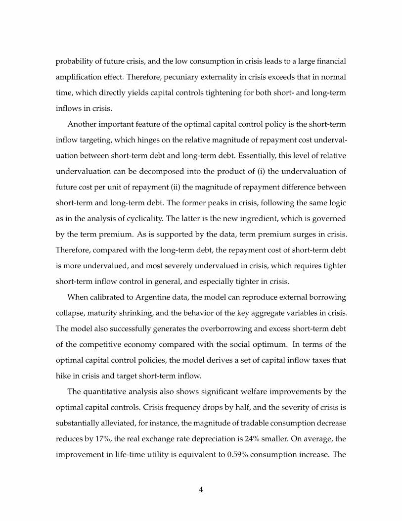
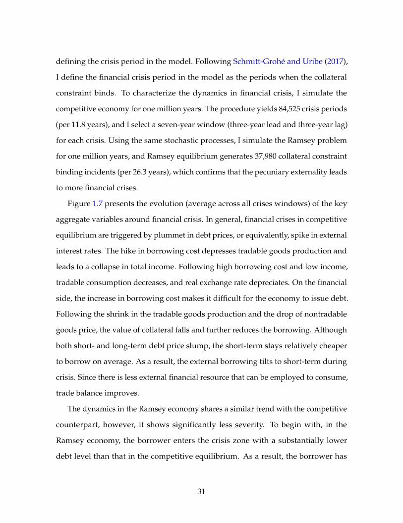
Figure 1.7 presents the evolution (average across all crises windows) of the key

aggregate variables around financial crisis. In general, financial crises in competitive

equilibrium are triggered by plummet in debt prices, or equivalently, spike in external

interest rates. The hike in borrowing cost depresses tradable goods production and

leads to a collapse in total income. Following high borrowing cost and low income,

tradable consumption decreases, and real exchange rate depreciates. On the financial

side, the increase in borrowing cost makes it difficult for the economy to issue debt.

Following the shrink in the tradable goods production and the drop of nontradable

goods price, the value of collateral falls and further reduces the borrowing. Although

both short- and long-term debt price slump, the short-term stays relatively cheaper

to borrow on average. As a result, the external borrowing tilts to short-term during

crisis. Since there is less external financial resource that can be employed to consume,

trade balance improves.

The dynamics in the Ramsey economy shares a similar trend with the competitive

counterpart, however, it shows significantly less severity. To begin with, in the

Ramsey economy, the borrower enters the crisis zone with a substantially lower

debt level than that in the competitive equilibrium. As a result, the borrower has

31

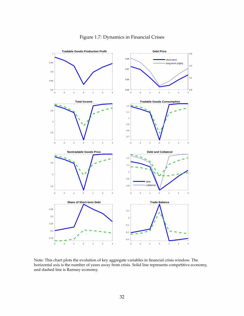
Figure 1.7: Dynamics in Financial Crises

-3 -2 -1 0 1 2 30.8

0.85

0.9

0.95

1Tradable Goods Production Profit

-3 -2 -1 0 1 2 30.83

0.85

0.87

0.89

Debt Price

2.9

3.1

3.3

3.5

short-term

long-term (right)

-3 -2 -1 0 1 2 3

2.5

3

3.5

Total Income

-3 -2 -1 0 1 2 3

0.7

0.8

0.9

1

1.1

1.2

Tradable Goods Consumption

-3 -2 -1 0 1 2 3

1.5

2

2.5

Nontradable Goods Price

-3 -2 -1 0 1 2 3

0.8

0.9

1

1.1

1.2

Debt and Collateral

debt

collateral

-3 -2 -1 0 1 2 3

0.15

0.2

0.25

0.3

0.35


-3 -2 -1 0 1 2 3

-0.3

-0.2

-0.1

0

0.1

Trade Balance

Note: This chart plots the evolution of key aggregate variables in financial crisis window. Thehorizontal axis is the number of years away from crisis. Solid line represents competitive economy,and dashed line is Ramsey economy.

32

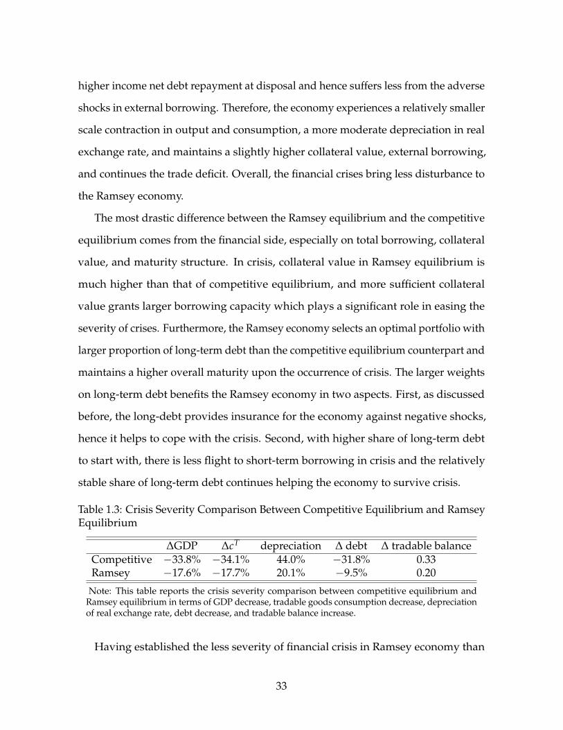
higher income net debt repayment at disposal and hence suffers less from the adverse

shocks in external borrowing. Therefore, the economy experiences a relatively smaller

scale contraction in output and consumption, a more moderate depreciation in real

exchange rate, and maintains a slightly higher collateral value, external borrowing,

and continues the trade deficit. Overall, the financial crises bring less disturbance to

the Ramsey economy.

The most drastic difference between the Ramsey equilibrium and the competitive

equilibrium comes from the financial side, especially on total borrowing, collateral

value, and maturity structure. In crisis, collateral value in Ramsey equilibrium is

much higher than that of competitive equilibrium, and more sufficient collateral

value grants larger borrowing capacity which plays a significant role in easing the

severity of crises. Furthermore, the Ramsey economy selects an optimal portfolio with

larger proportion of long-term debt than the competitive equilibrium counterpart and

maintains a higher overall maturity upon the occurrence of crisis. The larger weights

on long-term debt benefits the Ramsey economy in two aspects. First, as discussed

before, the long-debt provides insurance for the economy against negative shocks,

hence it helps to cope with the crisis. Second, with higher share of long-term debt

to start with, there is less flight to short-term borrowing in crisis and the relatively

stable share of long-term debt continues helping the economy to survive crisis.

Table 1.3: Crisis Severity Comparison Between Competitive Equilibrium and RamseyEquilibrium

∆GDP ∆cT depreciation ∆ debt ∆ tradable balanceCompetitive −33.8% −34.1% 44.0% −31.8% 0.33Ramsey −17.6% −17.7% 20.1% −9.5% 0.20

Note: This table reports the crisis severity comparison between competitive equilibrium andRamsey equilibrium in terms of GDP decrease, tradable goods consumption decrease, depreciationof real exchange rate, debt decrease, and tradable balance increase.

Having established the less severity of financial crisis in Ramsey economy than

33

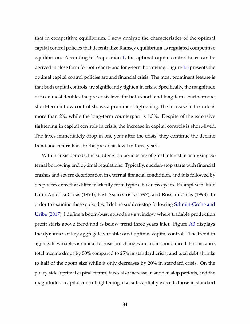
that in competitive equilibrium, I now analyze the characteristics of the optimal

capital control policies that decentralize Ramsey equilibrium as regulated competitive

equilibrium. According to Proposition 1, the optimal capital control taxes can be

derived in close form for both short- and long-term borrowing. Figure 1.8 presents the

optimal capital control policies around financial crisis. The most prominent feature is

that both capital controls are significantly tighten in crisis. Specifically, the magnitude

of tax almost doubles the pre-crisis level for both short- and long-term. Furthermore,

short-term inflow control shows a prominent tightening: the increase in tax rate is

more than 2%, while the long-term counterpart is 1.5%. Despite of the extensive

tightening in capital controls in crisis, the increase in capital controls is short-lived.

The taxes immediately drop in one year after the crisis, they continue the decline

trend and return back to the pre-crisis level in three years.

Within crisis periods, the sudden-stop periods are of great interest in analyzing ex-

ternal borrowing and optimal regulations. Typically, sudden-stop starts with financial

crashes and severe deterioration in external financial condidtion, and it is followed by

deep recessions that differ markedly from typical business cycles. Examples include

Latin America Crisis (1994), East Asian Crisis (1997), and Russian Crisis (1998). In

order to examine these episodes, I define sudden-stop following Schmitt-Grohé and

Uribe (2017), I define a boom-bust episode as a window where tradable production

profit starts above trend and is below trend three years later. Figure A3 displays

the dynamics of key aggregate variables and optimal capital controls. The trend in

aggregate variables is similar to crisis but changes are more pronounced. For instance,

total income drops by 50% compared to 25% in standard crisis, and total debt shrinks

to half of the boom size while it only decreases by 20% in standard crisis. On the

policy side, optimal capital control taxes also increase in sudden stop periods, and the

magnitude of capital control tightening also substantially exceeds those in standard

34

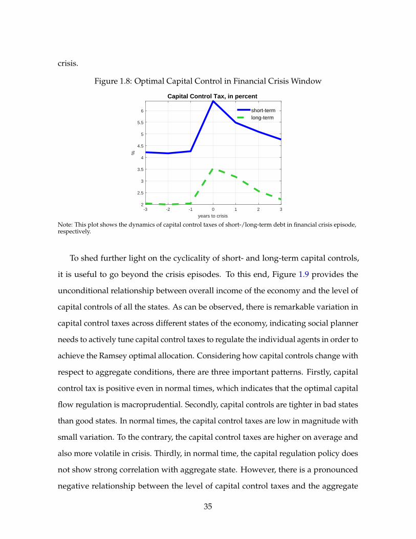
crisis.

Figure 1.8: Optimal Capital Control in Financial Crisis Window

-3 -2 -1 0 1 2 3

years to crisis

2

2.5

3

3.5

4

4.5

5

5.5

6

%

Capital Control Tax, in percent

short-termlong-term

Note: This plot shows the dynamics of capital control taxes of short-/long-term debt in financial crisis episode,respectively.

To shed further light on the cyclicality of short- and long-term capital controls,

it is useful to go beyond the crisis episodes. To this end, Figure 1.9 provides the

unconditional relationship between overall income of the economy and the level of

capital controls of all the states. As can be observed, there is remarkable variation in

capital control taxes across different states of the economy, indicating social planner

needs to actively tune capital control taxes to regulate the individual agents in order to

achieve the Ramsey optimal allocation. Considering how capital controls change with

respect to aggregate conditions, there are three important patterns. Firstly, capital

control tax is positive even in normal times, which indicates that the optimal capital

flow regulation is macroprudential. Secondly, capital controls are tighter in bad states

than good states. In normal times, the capital control taxes are low in magnitude with

small variation. To the contrary, the capital control taxes are higher on average and

also more volatile in crisis. Thirdly, in normal time, the capital regulation policy does

not show strong correlation with aggregate state. However, there is a pronounced

negative relationship between the level of capital control taxes and the aggregate

35

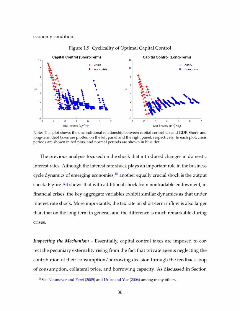
economy condition.

Figure 1.9: Cyclicality of Optimal Capital Control

Note: This plot shows the unconditional relationship between capital control tax and GDP. Short- andlong-term debt taxes are plotted on the left panel and the right panel, respectively. In each plot, crisisperiods are shown in red plus, and normal periods are shown in blue dot.

The previous analysis focused on the shock that introduced changes in domestic

interest rates. Although the interest rate shock plays an important role in the business

cycle dynamics of emerging economies,16 another equally crucial shock is the output

shock. Figure A4 shows that with additional shock from nontradable endowment, in

financial crises, the key aggregate variables exhibit similar dynamics as that under

interest rate shock. More importantly, the tax rate on short-term inflow is also larger

than that on the long-term in general, and the difference is much remarkable during

crises.

Inspecting the Mechanism – Essentially, capital control taxes are imposed to cor-

rect the pecuniary externality rising from the fact that private agents neglecting the

contribution of their consumption/borrowing decision through the feedback loop

of consumption, collateral price, and borrowing capacity. As discussed in Section

16See Neumeyer and Perri (2005) and Uribe and Yue (2006) among many others.

36

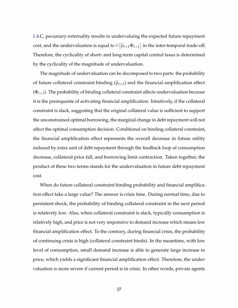
1.4.C, pecuniary externality results in undervaluing the expected future repayment

cost, and the undervaluation is equal to E[µt+1Φt+1

]in the inter-temporal trade-off.

Therefore, the cyclicality of short- and long-term capital control taxes is determined

by the cyclicality of the magnitude of undervaluation.

The magnitude of undervaluation can be decomposed to two parts: the probability

of future collateral constraint binding (µt+1) and the financial amplification effect

(Φt+1). The probability of binding collateral constraint affects undervaluation because

it is the prerequisite of activating financial amplification. Intuitively, if the collateral

constraint is slack, suggesting that the original collateral value is sufficient to support

the unconstrained optimal borrowing, the marginal change in debt repayment will not

affect the optimal consumption decision. Conditional on binding collateral constraint,

the financial amplification effect represents the overall decrease in future utility

induced by extra unit of debt repayment through the feedback loop of consumption

decrease, collateral price fall, and borrowing limit contraction. Taken together, the

product of these two terms stands for the undervaluation in future debt repayment

cost.

When do future collateral constraint binding probability and financial amplifica-

tion effect take a large value? The answer is crisis time. During normal time, due to

persistent shock, the probability of binding collateral constraint in the next period

is relatively low. Also, when collateral constraint is slack, typically consumption is

relatively high, and price is not very responsive to demand increase which means low

financial amplification effect. To the contrary, during financial crisis, the probability

of continuing crisis is high (collateral constraint binds). In the meantime, with low

level of consumption, small demand increase is able to generate large increase in

price, which yields a significant financial amplification effect. Therefore, the under-

valuation is more severe if current period is in crisis. In other words, private agents

37

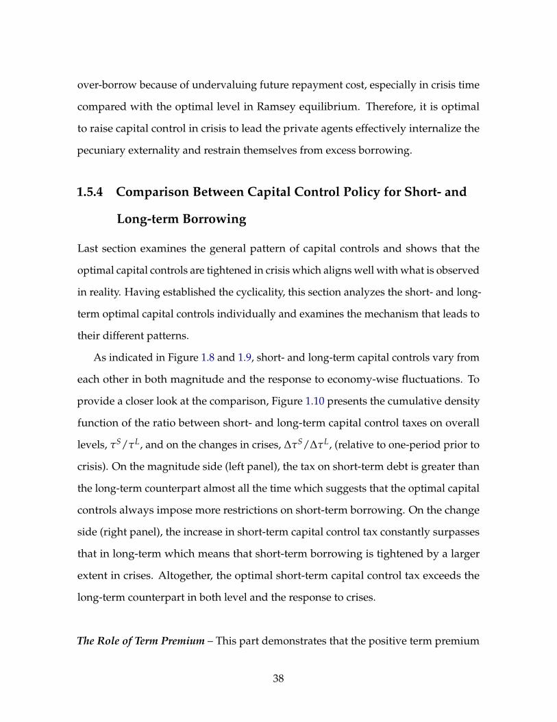
over-borrow because of undervaluing future repayment cost, especially in crisis time

compared with the optimal level in Ramsey equilibrium. Therefore, it is optimal

to raise capital control in crisis to lead the private agents effectively internalize the

pecuniary externality and restrain themselves from excess borrowing.

1.5.4 Comparison Between Capital Control Policy for Short- and

Long-term Borrowing

Last section examines the general pattern of capital controls and shows that the

optimal capital controls are tightened in crisis which aligns well with what is observed

in reality. Having established the cyclicality, this section analyzes the short- and long-

term optimal capital controls individually and examines the mechanism that leads to

their different patterns.

As indicated in Figure 1.8 and 1.9, short- and long-term capital controls vary from

each other in both magnitude and the response to economy-wise fluctuations. To

provide a closer look at the comparison, Figure 1.10 presents the cumulative density

function of the ratio between short- and long-term capital control taxes on overall

levels, τS/τL, and on the changes in crises, ∆τS/∆τL, (relative to one-period prior to

crisis). On the magnitude side (left panel), the tax on short-term debt is greater than

the long-term counterpart almost all the time which suggests that the optimal capital

controls always impose more restrictions on short-term borrowing. On the change

side (right panel), the increase in short-term capital control tax constantly surpasses

that in long-term which means that short-term borrowing is tightened by a larger

extent in crises. Altogether, the optimal short-term capital control tax exceeds the

long-term counterpart in both level and the response to crises.

The Role of Term Premium – This part demonstrates that the positive term premium

38

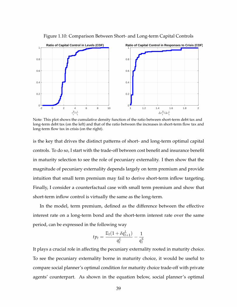
Figure 1.10: Comparison Between Short- and Long-term Capital Controls

-2 0 2 4 6 8 10

tS/

tL

0

0.2

0.4

0.6

0.8

1Ratio of Capital Control in Levels (CDF)

1 1.2 1.4 1.6 1.8 2

tS/

tL

0

0.2

0.4

0.6

0.8

1Ratio of Capital Control in Responses to Crisis (CDF)

Note: This plot shows the cumulative density function of the ratio between short-term debt tax andlong-term debt tax (on the left) and that of the ratio between the increases in short-term flow tax andlong-term flow tax in crisis (on the right).

is the key that drives the distinct patterns of short- and long-term optimal capital

controls. To do so, I start with the trade-off between cost benefit and insurance benefit

in maturity selection to see the role of pecuniary externality. I then show that the

magnitude of pecuniary externality depends largely on term premium and provide

intuition that small term premium may fail to derive short-term inflow targeting.

Finally, I consider a counterfactual case with small term premium and show that

short-term inflow control is virtually the same as the long-term.

In the model, term premium, defined as the difference between the effective

interest rate on a long-term bond and the short-term interest rate over the same

period, can be expressed in the following way

tpt =Et(1 + δqL

t+1)

qLt

− 1qS

t

It plays a crucial role in affecting the pecuniary externality rooted in maturity choice.

To see the pecuniary externality borne in maturity choice, it would be useful to

compare social planner’s optimal condition for maturity choice trade-off with private

agents’ counterpart. As shown in the equation below, social planner’s optimal

39

condition contains an extra term, Et[µt+1Φt+1(1 + δqL

t+1 −qL

tqS

t)], in the insurance

benefit of long-term debt. This term is precisely pecuniary externality.

Et

[u′Tt+1

( 1qS

t−

1 + δqLt+1

qLt

)]+ Et

[µt+1Φt+1

( 1qS

t−

1 + δqLt+1

qLt

)]= 0

Et

[u′Tt+1 · tpt

]+ Et

[µt+1Φt+1 · tpt

]= 0

What does the pecuniary externality term stand for in the insurance benefit of

long-term debt? Fundamentally, insurance benefit of long-term debt stems from the

fact that long-term debt’s effectively repayment is smaller than that of short-term

debt in bad states, bringing in resource to future adverse states, as confirmed by

Figure 1.5. The pecuniary externality term, Et[µt+1Φt+1(1 + δqL

t+1 −qL

tqS

t)], captures

difference between the undervaluation of repayment cost associated with short-term

debt and long-term debt, and this relative cost undervaluation leads to inefficient

maturity structure and calls for maturity-dependent capital control policies.

To shed light on the extent of maturity-dependence and how short- and long-

term inflow controls should differ from each other, it is important to analyze the

variation in the magnitude of the relative cost undervaluation between short-term

debt and long-term debt along business cycle. Basically, the pecuniary externality

here represents the expected marginal utility from swapping to long-term borrowing

through the collateral price and borrowing limit feedback loop. Therefore, the total

pecuniary externality can be decomposed to two parts: one is the undervaluation

of future repayment cost per unit of repayment, and the other is the amount of

repayment decrease due to the insurance benefit of long-term debt. As shown in

the cyclicality of capital control, the first component peaks in crisis due to the large

probability of collateral constraint binding and the significant magnitude of financial

amplification. The second component, which is unique to maturity structure choice,

is determined by term premium. Therefore, the higher the term premium is, the

40

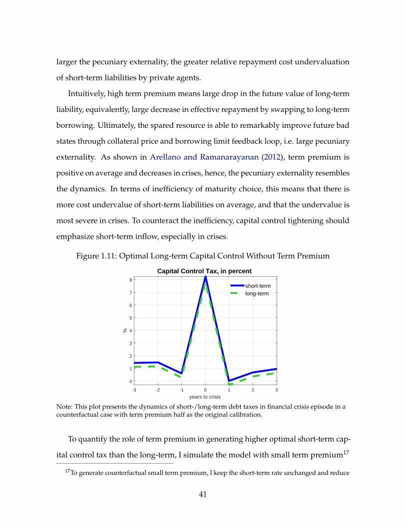
larger the pecuniary externality, the greater relative repayment cost undervaluation

of short-term liabilities by private agents.

Intuitively, high term premium means large drop in the future value of long-term

liability, equivalently, large decrease in effective repayment by swapping to long-term

borrowing. Ultimately, the spared resource is able to remarkably improve future bad

states through collateral price and borrowing limit feedback loop, i.e. large pecuniary

externality. As shown in Arellano and Ramanarayanan (2012), term premium is

positive on average and decreases in crises, hence, the pecuniary externality resembles

the dynamics. In terms of inefficiency of maturity choice, this means that there is

more cost undervalue of short-term liabilities on average, and that the undervalue is

most severe in crises. To counteract the inefficiency, capital control tightening should

emphasize short-term inflow, especially in crises.

Figure 1.11: Optimal Long-term Capital Control Without Term Premium

-3 -2 -1 0 1 2 3

years to crisis

0

1

2

3

4

5

6

7

8

%


short-termlong-term

Note: This plot presents the dynamics of short-/long-term debt taxes in financial crisis episode in acounterfactual case with term premium half as the original calibration.

To quantify the role of term premium in generating higher optimal short-term cap-

ital control tax than the long-term, I simulate the model with small term premium17

17To generate counterfactual small term premium, I keep the short-term rate unchanged and reduce

41

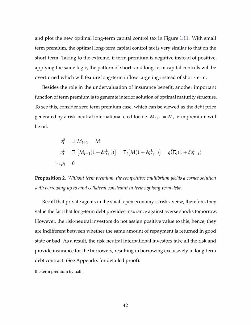
and plot the new optimal long-term capital control tax in Figure 1.11. With small

term premium, the optimal long-term capital control tax is very similar to that on the

short-term. Taking to the extreme, if term premium is negative instead of positive,

applying the same logic, the pattern of short- and long-term capital controls will be

overturned which will feature long-term inflow targeting instead of short-term.

Besides the role in the undervaluation of insurance benefit, another important

function of term premium is to generate interior solution of optimal maturity structure.

To see this, consider zero term premium case, which can be viewed as the debt price

generated by a risk-neutral international creditor, i.e. Mt+1 = M, term premium will

be nil.

qSt = EtMt+1 = M

qLt = Et

[Mt+1(1 + δqL

t+1)]= Et

[M(1 + δqL

t+1)]= qS

t Et(1 + δqLt+1)

=⇒ tpt = 0

Proposition 2. Without term premium, the competitive equilibrium yields a corner solution

with borrowing up to bind collateral constraint in terms of long-term debt.

Recall that private agents in the small open economy is risk-averse, therefore, they

value the fact that long-term debt provides insurance against averse shocks tomorrow.

However, the risk-neutral investors do not assign positive value to this, hence, they

are indifferent between whether the same amount of repayment is returned in good

state or bad. As a result, the risk-neutral international investors take all the risk and

provide insurance for the borrowers, resulting in borrowing exclusively in long-term

debt contract. (See Appendix for detailed proof).

the term premium by half.

42

1.5.5 Debt Portfolio In Competitive Equilibrium and Ramsey

Equilibrium

As shown in Section 1.4.C, Ramsey equilibrium has fewer crises and less severe crises,

and one important difference between the two is the external borrowing decision. In

Ramsey equilibrium, total borrowing falls less than that in competitive equilibrium,

and the share of short-term debt is much smaller. This section aims to provide more

information on the comparison on the debt portfolio between the two types of equi-

libria, going beyond the crisis episodes.

Total Debt – Social planner and private agents differ in their calculation of the ex-

pected future repayment cost, and this difference will be factored into the optimal

total borrowing and result in different debt volume. To analyze the choice of debt

volume in competitive equilibrium and Ramsey equilibrium, I compare the total

debt’s ergodic distribution in the two equilibria. Since social planner internalizes the

financial amplification effect of future repayment cost through the feedback loop of

consumption decrease, collateral price fall, and borrowing capacity contract, social

planner restrains from over consume today and takes a less indebted position than

private agent.

To demonstrate the correction of over-borrowing by optimal capital controls,

Figure 1.12 (left panel) plots the ergodic distribution of total debt accumulation in

Ramsey economy and competitive economy, respectively. The pattern implies that

the competitive economy assign higher probability to holding large amount of debt.

The average total debt stock in competitive economy (0.89) is significantly higher

than the Ramsey economy counterpart (0.79).

Debt Maturity – Another important aspect of debt policy is the maturity choice.

43

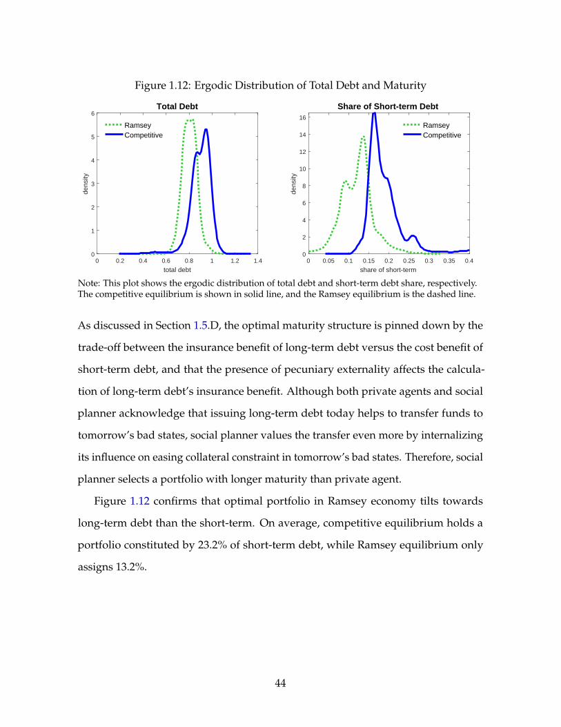
Figure 1.12: Ergodic Distribution of Total Debt and Maturity

0 0.2 0.4 0.6 0.8 1 1.2 1.4

total debt

0

1

2

3

4

5

6

dens

ity

Total Debt

RamseyCompetitive

0 0.05 0.1 0.15 0.2 0.25 0.3 0.35 0.4

share of short-term

0

2

4

6

8

10

12

14

16

dens

ity


RamseyCompetitive

Note: This plot shows the ergodic distribution of total debt and short-term debt share, respectively.The competitive equilibrium is shown in solid line, and the Ramsey equilibrium is the dashed line.

As discussed in Section 1.5.D, the optimal maturity structure is pinned down by the

trade-off between the insurance benefit of long-term debt versus the cost benefit of

short-term debt, and that the presence of pecuniary externality affects the calcula-

tion of long-term debt’s insurance benefit. Although both private agents and social

planner acknowledge that issuing long-term debt today helps to transfer funds to

tomorrow’s bad states, social planner values the transfer even more by internalizing

its influence on easing collateral constraint in tomorrow’s bad states. Therefore, social

planner selects a portfolio with longer maturity than private agent.

Figure 1.12 confirms that optimal portfolio in Ramsey economy tilts towards

long-term debt than the short-term. On average, competitive equilibrium holds a

portfolio constituted by 23.2% of short-term debt, while Ramsey equilibrium only

assigns 13.2%.

44

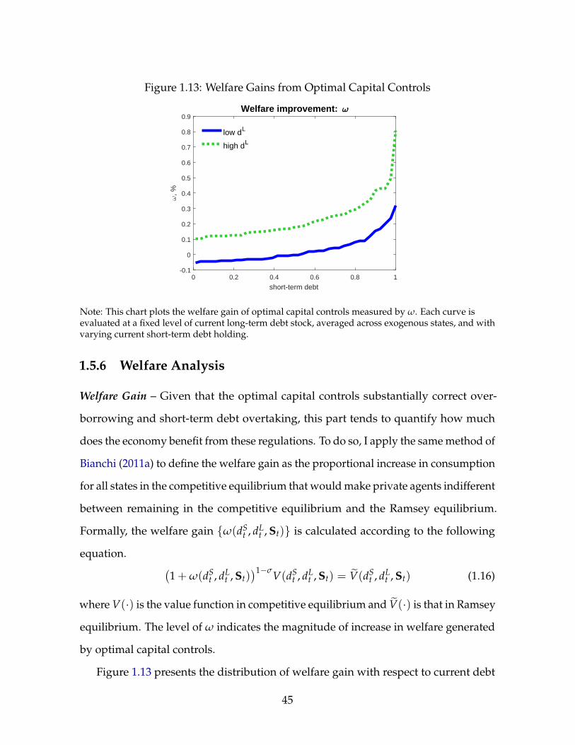
Figure 1.13: Welfare Gains from Optimal Capital Controls

0 0.2 0.4 0.6 0.8 1

short-term debt

-0.1

0

0.1

0.2

0.3

0.4

0.5

0.6

0.7

0.8

0.9

, %

Welfare improvement:

low dL

high dL

Note: This chart plots the welfare gain of optimal capital controls measured by ω. Each curve isevaluated at a fixed level of current long-term debt stock, averaged across exogenous states, and withvarying current short-term debt holding.

1.5.6 Welfare Analysis

Welfare Gain – Given that the optimal capital controls substantially correct over-

borrowing and short-term debt overtaking, this part tends to quantify how much

does the economy benefit from these regulations. To do so, I apply the same method of

Bianchi (2011a) to define the welfare gain as the proportional increase in consumption

for all states in the competitive equilibrium that would make private agents indifferent

between remaining in the competitive equilibrium and the Ramsey equilibrium.

Formally, the welfare gain {ω(dSt , dL

t , St)} is calculated according to the following

equation. (1 + ω(dS

t , dLt , St)

)1−σV(dSt , dL

t , St) = V(dSt , dL

t , St) (1.16)

where V(·) is the value function in competitive equilibrium and V(·) is that in Ramsey

equilibrium. The level of ω indicates the magnitude of increase in welfare generated

by optimal capital controls.

Figure 1.13 presents the distribution of welfare gain with respect to current debt

45

levels. First, for the majority cases, optimal capital control policies improves welfare

as expected, no matter starting with low liability or high debt burden. Second, the

magnitude of welfare improvement is positively correlated with the level of debt.

Intuitively, with high level of debt, the economy is vulnerable to future adverse

shocks and results in crisis. In these states, the optimal capital controls has the largest

correction effect in constraining over-borrowing and preventing crisis. Thirdly, as has

been shown that crises periods require higher capital control tax rates, a suboptimal

constant tax rate must lie between the lower level in tranquil times and the higher

level in crises times. As a result, the high tax rate may discourage consumption and

borrowing in states with favorable borrowing conditions. For instance, in Figure 1.13,

with low liabilities, meaning decent financial outstanding, welfare gain is slightly

negative. All the states taken together, the optimal capital controls raise welfare

equivalent to 0.59% increase in consumption on average.

The previous sections have established that the Ramsey equilibrium can be sup-

ported by a set of state-contingent and maturity-dependent capital controls in the

competitive equilibrium, and that the optimal capital controls significantly improve

welfare. Given the significant welfare enhancement of optimal policies, this section

analyzes the welfare effect under sub-optimal policies, i.e. state-independent or

maturity-independent. To do so, I consider the same environment as the benchmark

but limit social planner to be able to use only fixed-rate capital control taxes. In partic-

ular, I consider four cases: i) fixed taxes but maturity-dependent (τSt = τS, τL

t = τL), ii)

fixed tax and maturity-independent (τSt = τL

t = τ), iii) only fixed tax on short-term in-

flow (τSt = τS, τL

t = 0), and iv) only fixed tax on long-term inflow (τSt = 0, τL

t = τL).18

In general, these cases tend to provide insights on policy implementations when reg-

ulations are challenging to implement in practice, in particular, the last two are also

18Ideally, another case with state-contingent but maturity-independent taxes should be considered,however, the solution of constrained optimal taxes is difficult given the large number of states.

46

set to gauge the relative importance of short- and long-term inflow capital controls.

Without state-dependent capital control taxes, the decentralization of Ramsey

equilibrium is no longer feasible. Consequently, social planner now solves for the

optimal level of fixed capital control tax to maximize household’s expected life-

time utility with the post-tax borrowing rates. Since the state-contingent optimal

capital controls is procyclical, if set equally, social planner trades off between the

benefit of high tax rate in preventing crisis and the corresponding cost in depressing

consumption in normal time.

Definition 5. (Constrained Social Planner’s Optimization Problem) Social planner chooses

τ to maximize the value function resulted from the competitive equilibrium accordingly to

Definition 1 under the post-tax effective borrowing rates.

Table 1.4 presents the welfare effect of different types of capital controls compared

to the unregulated competitive benchmark. The first observation is that the optimal

capital control tax, even set fixed, is able to insure the economy against adverse

shocks, reduce crisis frequency, and improve welfare on average. For instance, the

maturity-dependent fixed taxes are able to achieve 59% of the welfare improvement

under optimal capital controls, and even the least effective one, fixed tax on long-term

inflow, generates positive welfare improvement. This result is reasonable given that

in the model, pecuniary externality calls for positive tax rate even in normal time.

Second, state-contingency contributes a significant part of welfare improvement.

From the optimal case to state-independent case i), the welfare gain drops by 40%.

However, from the maturity-dependent case i) to maturity-independent case ii), the

welfare gain drops by a smaller extent, 13%.

Regarding the individual effectiveness of short-term inflow control and long-term

inflow control, if restricted with one type of fixed tax, the economy will benefit more

from a fixed short-term capital control tax. The flat short-term capital control tax is

47

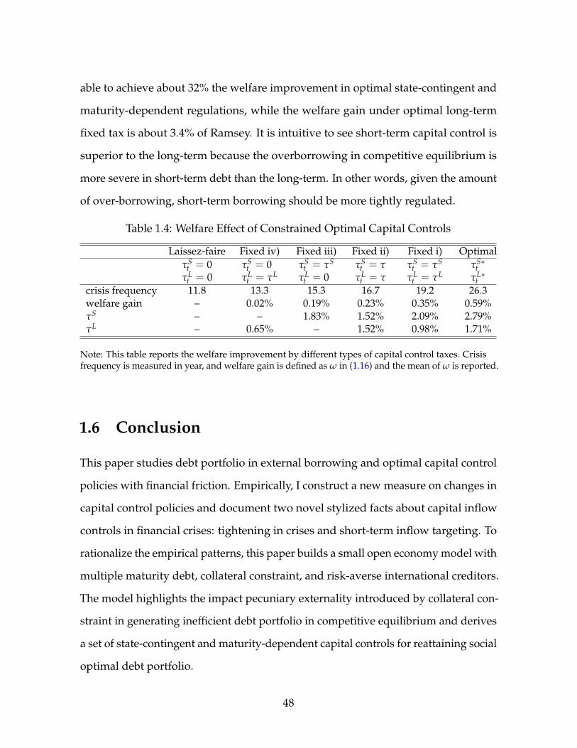
able to achieve about 32% the welfare improvement in optimal state-contingent and

maturity-dependent regulations, while the welfare gain under optimal long-term

fixed tax is about 3.4% of Ramsey. It is intuitive to see short-term capital control is

superior to the long-term because the overborrowing in competitive equilibrium is

more severe in short-term debt than the long-term. In other words, given the amount

of over-borrowing, short-term borrowing should be more tightly regulated.

Table 1.4: Welfare Effect of Constrained Optimal Capital Controls

Laissez-faire Fixed iv) Fixed iii) Fixed ii) Fixed i) OptimalτS

t = 0τL

t = 0τS

t = 0τL

t = τLτS

t = τS

τLt = 0

τSt = τ

τLt = τ

τSt = τS

τLt = τL

τS∗t

τL∗t

crisis frequency 11.8 13.3 15.3 16.7 19.2 26.3welfare gain – 0.02% 0.19% 0.23% 0.35% 0.59%τS – – 1.83% 1.52% 2.09% 2.79%τL – 0.65% – 1.52% 0.98% 1.71%

Note: This table reports the welfare improvement by different types of capital control taxes. Crisisfrequency is measured in year, and welfare gain is defined as ω in (1.16) and the mean of ω is reported.

1.6 Conclusion

This paper studies debt portfolio in external borrowing and optimal capital control

policies with financial friction. Empirically, I construct a new measure on changes in

capital control policies and document two novel stylized facts about capital inflow

controls in financial crises: tightening in crises and short-term inflow targeting. To

rationalize the empirical patterns, this paper builds a small open economy model with

multiple maturity debt, collateral constraint, and risk-averse international creditors.

The model highlights the impact pecuniary externality introduced by collateral con-

straint in generating inefficient debt portfolio in competitive equilibrium and derives

a set of state-contingent and maturity-dependent capital controls for reattaining social

optimal debt portfolio.

48

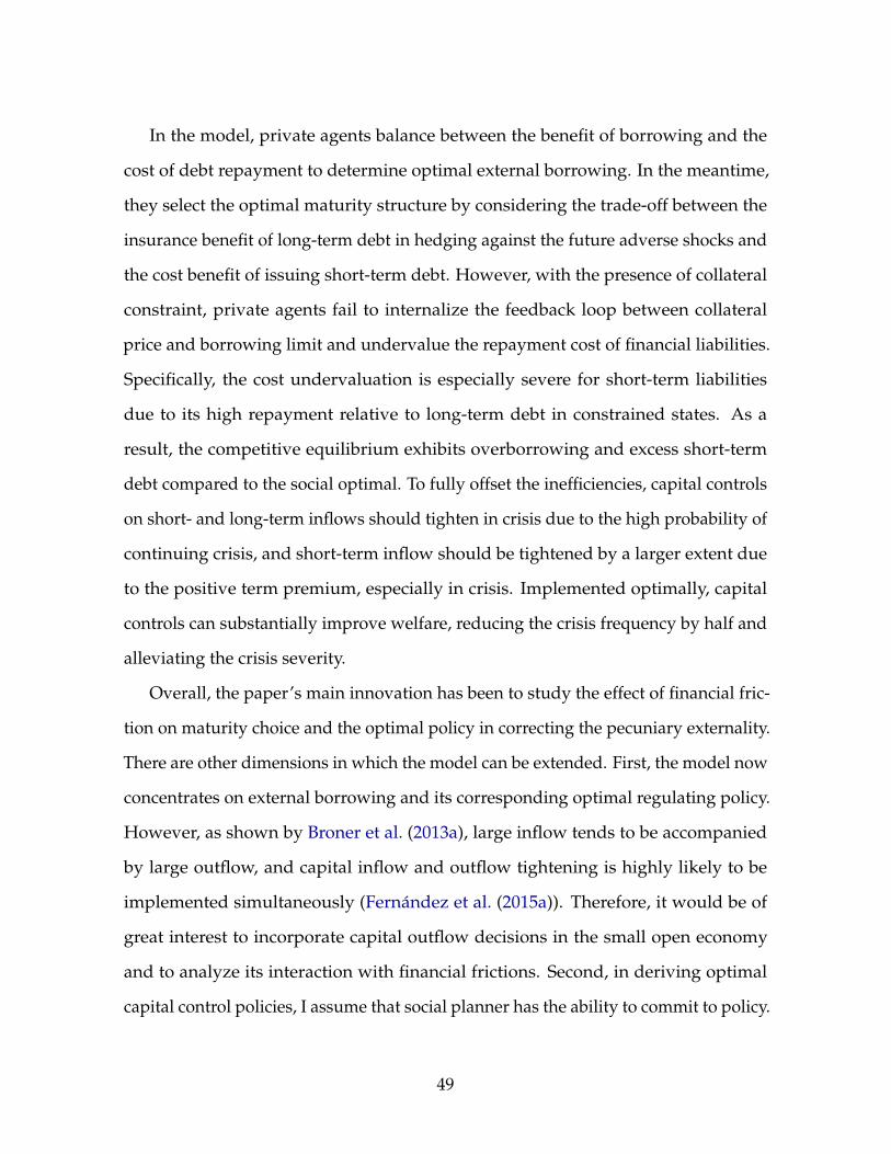
In the model, private agents balance between the benefit of borrowing and the

cost of debt repayment to determine optimal external borrowing. In the meantime,

they select the optimal maturity structure by considering the trade-off between the

insurance benefit of long-term debt in hedging against the future adverse shocks and

the cost benefit of issuing short-term debt. However, with the presence of collateral

constraint, private agents fail to internalize the feedback loop between collateral

price and borrowing limit and undervalue the repayment cost of financial liabilities.

Specifically, the cost undervaluation is especially severe for short-term liabilities

due to its high repayment relative to long-term debt in constrained states. As a

result, the competitive equilibrium exhibits overborrowing and excess short-term

debt compared to the social optimal. To fully offset the inefficiencies, capital controls

on short- and long-term inflows should tighten in crisis due to the high probability of

continuing crisis, and short-term inflow should be tightened by a larger extent due

to the positive term premium, especially in crisis. Implemented optimally, capital

controls can substantially improve welfare, reducing the crisis frequency by half and

alleviating the crisis severity.

Overall, the paper’s main innovation has been to study the effect of financial fric-

tion on maturity choice and the optimal policy in correcting the pecuniary externality.

There are other dimensions in which the model can be extended. First, the model now

concentrates on external borrowing and its corresponding optimal regulating policy.

However, as shown by Broner et al. (2013a), large inflow tends to be accompanied

by large outflow, and capital inflow and outflow tightening is highly likely to be

implemented simultaneously (Fernández et al. (2015a)). Therefore, it would be of

great interest to incorporate capital outflow decisions in the small open economy

and to analyze its interaction with financial frictions. Second, in deriving optimal

capital control policies, I assume that social planner has the ability to commit to policy.

49

This might change under different forms of collateral such as asset. To examine the

Markov perfect equilibrium with external borrowing at different maturities would be

an important complement to the study in this paper.

50

Chapter 2

Capital Controls in Financial Crises: An Empirical Analysis

51

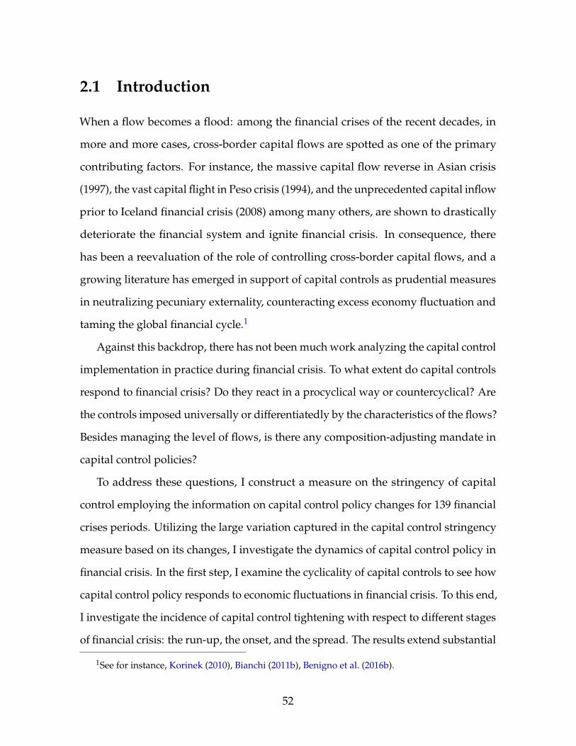
2.1 Introduction

When a flow becomes a flood: among the financial crises of the recent decades, in

more and more cases, cross-border capital flows are spotted as one of the primary

contributing factors. For instance, the massive capital flow reverse in Asian crisis

(1997), the vast capital flight in Peso crisis (1994), and the unprecedented capital inflow

prior to Iceland financial crisis (2008) among many others, are shown to drastically

deteriorate the financial system and ignite financial crisis. In consequence, there

has been a reevaluation of the role of controlling cross-border capital flows, and a

growing literature has emerged in support of capital controls as prudential measures

in neutralizing pecuniary externality, counteracting excess economy fluctuation and

taming the global financial cycle.1

Against this backdrop, there has not been much work analyzing the capital control

implementation in practice during financial crisis. To what extent do capital controls

respond to financial crisis? Do they react in a procyclical way or countercyclical? Are

the controls imposed universally or differentiatedly by the characteristics of the flows?

Besides managing the level of flows, is there any composition-adjusting mandate in

capital control policies?

To address these questions, I construct a measure on the stringency of capital

control employing the information on capital control policy changes for 139 financial

crises periods. Utilizing the large variation captured in the capital control stringency

measure based on its changes, I investigate the dynamics of capital control policy in

financial crisis. In the first step, I examine the cyclicality of capital controls to see how

capital control policy responds to economic fluctuations in financial crisis. To this end,

I investigate the incidence of capital control tightening with respect to different stages

of financial crisis: the run-up, the onset, and the spread. The results extend substantial

1See for instance, Korinek (2010), Bianchi (2011b), Benigno et al. (2016b).

52

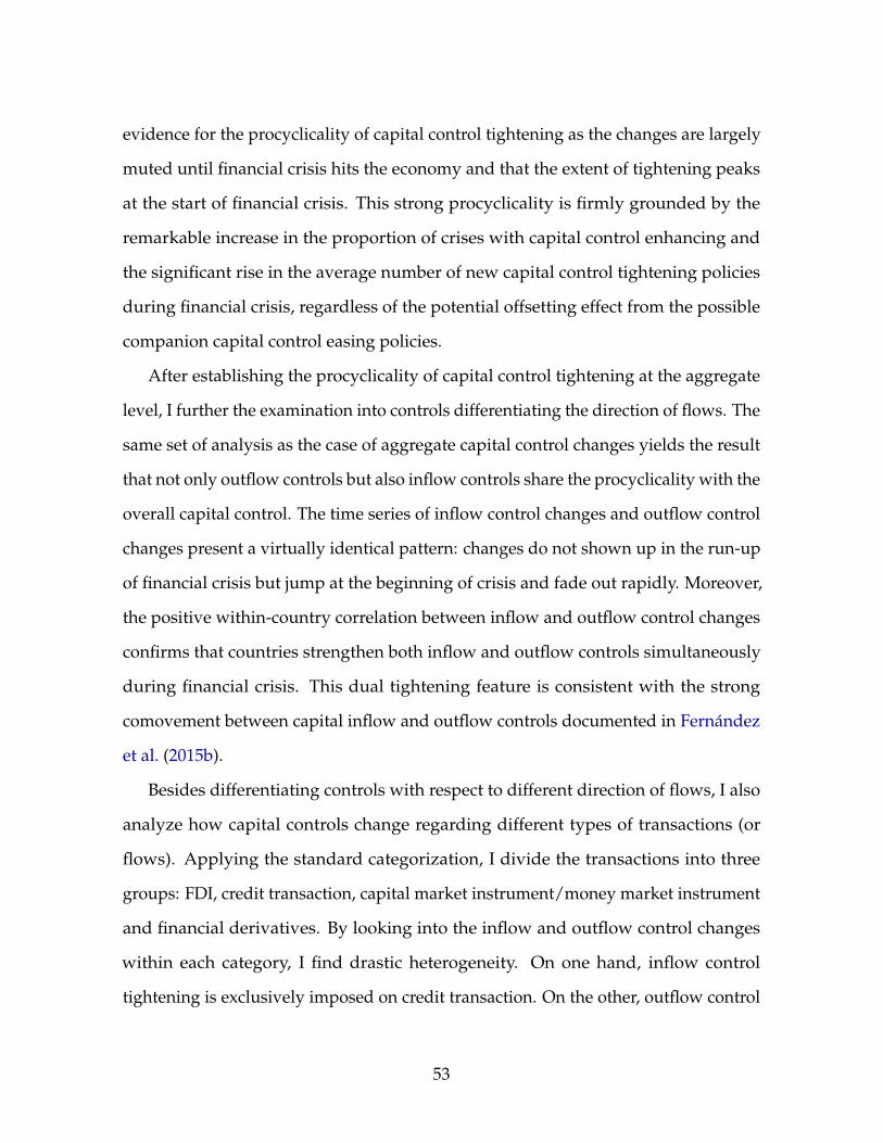
evidence for the procyclicality of capital control tightening as the changes are largely

muted until financial crisis hits the economy and that the extent of tightening peaks

at the start of financial crisis. This strong procyclicality is firmly grounded by the

remarkable increase in the proportion of crises with capital control enhancing and

the significant rise in the average number of new capital control tightening policies

during financial crisis, regardless of the potential offsetting effect from the possible

companion capital control easing policies.

After establishing the procyclicality of capital control tightening at the aggregate

level, I further the examination into controls differentiating the direction of flows. The

same set of analysis as the case of aggregate capital control changes yields the result

that not only outflow controls but also inflow controls share the procyclicality with the

overall capital control. The time series of inflow control changes and outflow control

changes present a virtually identical pattern: changes do not shown up in the run-up

of financial crisis but jump at the beginning of crisis and fade out rapidly. Moreover,

the positive within-country correlation between inflow and outflow control changes

confirms that countries strengthen both inflow and outflow controls simultaneously

during financial crisis. This dual tightening feature is consistent with the strong

comovement between capital inflow and outflow controls documented in Fernández

et al. (2015b).

Besides differentiating controls with respect to different direction of flows, I also

analyze how capital controls change regarding different types of transactions (or

flows). Applying the standard categorization, I divide the transactions into three

groups: FDI, credit transaction, capital market instrument/money market instrument

and financial derivatives. By looking into the inflow and outflow control changes

within each category, I find drastic heterogeneity. On one hand, inflow control

tightening is exclusively imposed on credit transaction. On the other, outflow control

53

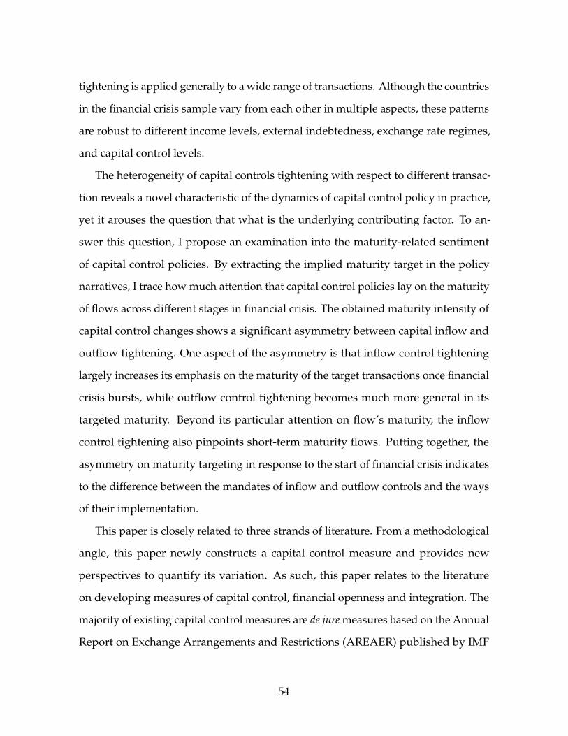
tightening is applied generally to a wide range of transactions. Although the countries

in the financial crisis sample vary from each other in multiple aspects, these patterns

are robust to different income levels, external indebtedness, exchange rate regimes,

and capital control levels.

The heterogeneity of capital controls tightening with respect to different transac-

tion reveals a novel characteristic of the dynamics of capital control policy in practice,

yet it arouses the question that what is the underlying contributing factor. To an-

swer this question, I propose an examination into the maturity-related sentiment

of capital control policies. By extracting the implied maturity target in the policy

narratives, I trace how much attention that capital control policies lay on the maturity

of flows across different stages in financial crisis. The obtained maturity intensity of

capital control changes shows a significant asymmetry between capital inflow and

outflow tightening. One aspect of the asymmetry is that inflow control tightening

largely increases its emphasis on the maturity of the target transactions once financial

crisis bursts, while outflow control tightening becomes much more general in its

targeted maturity. Beyond its particular attention on flow’s maturity, the inflow

control tightening also pinpoints short-term maturity flows. Putting together, the

asymmetry on maturity targeting in response to the start of financial crisis indicates

to the difference between the mandates of inflow and outflow controls and the ways

of their implementation.

This paper is closely related to three strands of literature. From a methodological

angle, this paper newly constructs a capital control measure and provides new

perspectives to quantify its variation. As such, this paper relates to the literature

on developing measures of capital control, financial openness and integration. The

majority of existing capital control measures are de jure measures based on the Annual

Report on Exchange Arrangements and Restrictions (AREAER) published by IMF

54

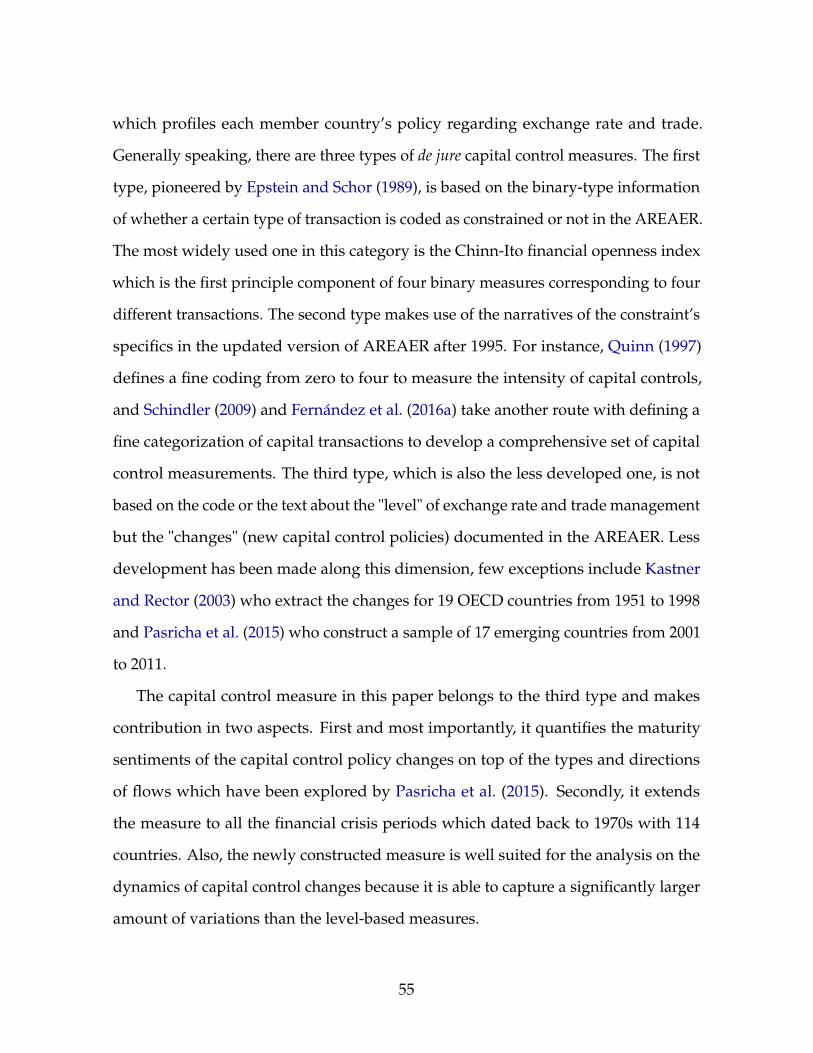
which profiles each member country’s policy regarding exchange rate and trade.

Generally speaking, there are three types of de jure capital control measures. The first

type, pioneered by Epstein and Schor (1989), is based on the binary-type information

of whether a certain type of transaction is coded as constrained or not in the AREAER.

The most widely used one in this category is the Chinn-Ito financial openness index

which is the first principle component of four binary measures corresponding to four

different transactions. The second type makes use of the narratives of the constraint’s

specifics in the updated version of AREAER after 1995. For instance, Quinn (1997)

defines a fine coding from zero to four to measure the intensity of capital controls,

and Schindler (2009) and Fernández et al. (2016a) take another route with defining a

fine categorization of capital transactions to develop a comprehensive set of capital

control measurements. The third type, which is also the less developed one, is not

based on the code or the text about the "level" of exchange rate and trade management

but the "changes" (new capital control policies) documented in the AREAER. Less

development has been made along this dimension, few exceptions include Kastner

and Rector (2003) who extract the changes for 19 OECD countries from 1951 to 1998

and Pasricha et al. (2015) who construct a sample of 17 emerging countries from 2001

to 2011.

The capital control measure in this paper belongs to the third type and makes

contribution in two aspects. First and most importantly, it quantifies the maturity

sentiments of the capital control policy changes on top of the types and directions

of flows which have been explored by Pasricha et al. (2015). Secondly, it extends

the measure to all the financial crisis periods which dated back to 1970s with 114

countries. Also, the newly constructed measure is well suited for the analysis on the

dynamics of capital control changes because it is able to capture a significantly larger

amount of variations than the level-based measures.

55

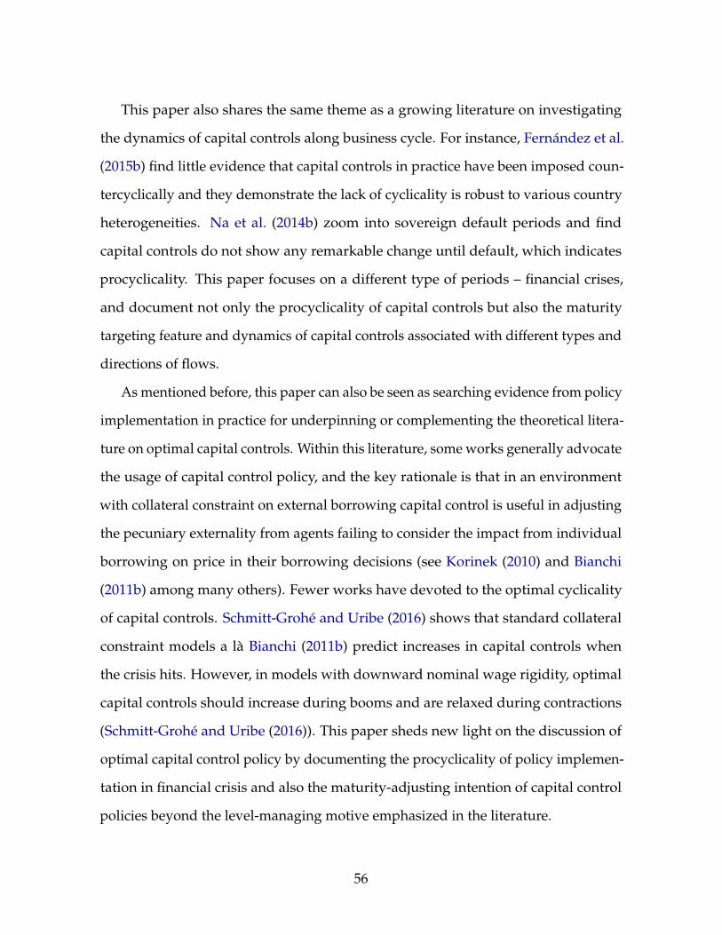
This paper also shares the same theme as a growing literature on investigating

the dynamics of capital controls along business cycle. For instance, Fernández et al.

(2015b) find little evidence that capital controls in practice have been imposed coun-

tercyclically and they demonstrate the lack of cyclicality is robust to various country

heterogeneities. Na et al. (2014b) zoom into sovereign default periods and find

capital controls do not show any remarkable change until default, which indicates

procyclicality. This paper focuses on a different type of periods – financial crises,

and document not only the procyclicality of capital controls but also the maturity

targeting feature and dynamics of capital controls associated with different types and

directions of flows.

As mentioned before, this paper can also be seen as searching evidence from policy

implementation in practice for underpinning or complementing the theoretical litera-

ture on optimal capital controls. Within this literature, some works generally advocate

the usage of capital control policy, and the key rationale is that in an environment

with collateral constraint on external borrowing capital control is useful in adjusting

the pecuniary externality from agents failing to consider the impact from individual

borrowing on price in their borrowing decisions (see Korinek (2010) and Bianchi

(2011b) among many others). Fewer works have devoted to the optimal cyclicality

of capital controls. Schmitt-Grohé and Uribe (2016) shows that standard collateral

constraint models a là Bianchi (2011b) predict increases in capital controls when

the crisis hits. However, in models with downward nominal wage rigidity, optimal

capital controls should increase during booms and are relaxed during contractions

(Schmitt-Grohé and Uribe (2016)). This paper sheds new light on the discussion of

optimal capital control policy by documenting the procyclicality of policy implemen-

tation in financial crisis and also the maturity-adjusting intention of capital control

policies beyond the level-managing motive emphasized in the literature.

56

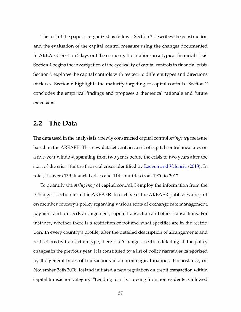
The rest of the paper is organized as follows. Section 2 describes the construction

and the evaluation of the capital control measure using the changes documented

in AREAER. Section 3 lays out the economy fluctuations in a typical financial crisis.

Section 4 begins the investigation of the cyclicality of capital controls in financial crisis.

Section 5 explores the capital controls with respect to different types and directions

of flows. Section 6 highlights the maturity targeting of capital controls. Section 7

concludes the empirical findings and proposes a theoretical rationale and future

extensions.

2.2 The Data

The data used in the analysis is a newly constructed capital control stringency measure

based on the AREAER. This new dataset contains a set of capital control measures on

a five-year window, spanning from two years before the crisis to two years after the

start of the crisis, for the financial crises identified by Laeven and Valencia (2013). In

total, it covers 139 financial crises and 114 countries from 1970 to 2012.

To quantify the stringency of capital control, I employ the information from the

"Changes" section from the AREAER. In each year, the AREAER publishes a report

on member country’s policy regarding various sorts of exchange rate management,

payment and proceeds arrangement, capital transaction and other transactions. For

instance, whether there is a restriction or not and what specifics are in the restric-

tion. In every country’s profile, after the detailed description of arrangements and

restrictions by transaction type, there is a "Changes" section detailing all the policy

changes in the previous year. It is constituted by a list of policy narratives categorized

by the general types of transactions in a chronological manner. For instance, on

November 28th 2008, Iceland initiated a new regulation on credit transaction within

capital transaction category: "Lending to or borrowing from nonresidents is allowed

57

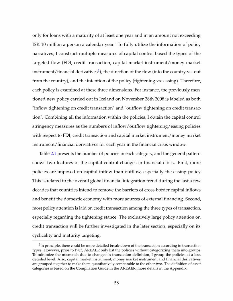
only for loans with a maturity of at least one year and in an amount not exceeding

ISK 10 million a person a calendar year." To fully utilize the information of policy

narratives, I construct multiple measures of capital control based the types of the

targeted flow (FDI, credit transaction, capital market instrument/money market

instrument/financial derivatives2), the direction of the flow (into the country vs. out

from the country), and the intention of the policy (tightening vs. easing). Therefore,

each policy is examined at these three dimensions. For instance, the previously men-

tioned new policy carried out in Iceland on November 28th 2008 is labeled as both

"inflow tightening on credit transaction" and "outflow tightening on credit transac-

tion". Combining all the information within the policies, I obtain the capital control

stringency measures as the numbers of inflow/outflow tightening/easing policies

with respect to FDI, credit transaction and capital market instrument/money market

instrument/financial derivatives for each year in the financial crisis window.

Table 2.1 presents the number of policies in each category, and the general pattern

shows two features of the capital control changes in financial crisis. First, more

policies are imposed on capital inflow than outflow, especially the easing policy.

This is related to the overall global financial integration trend during the last a few

decades that countries intend to remove the barriers of cross-border capital inflows

and benefit the domestic economy with more sources of external financing. Second,

most policy attention is laid on credit transaction among the three types of transaction,

especially regarding the tightening stance. The exclusively large policy attention on

credit transaction will be further investigated in the later section, especially on its

cyclicality and maturity targeting.

2In principle, there could be more detailed break-down of the transaction according to transactiontypes. However, prior to 1983, AREAER only list the policies without categorizing them into groups.To minimize the mismatch due to changes in transaction definition, I group the policies at a lessdetailed level. Also, capital market instrument, money market instrument and financial derivativesare grouped together to make them quantitatively comparable to the other two. The definition of assetcategories is based on the Compilation Guide in the AREAER, more details in the Appendix.

58

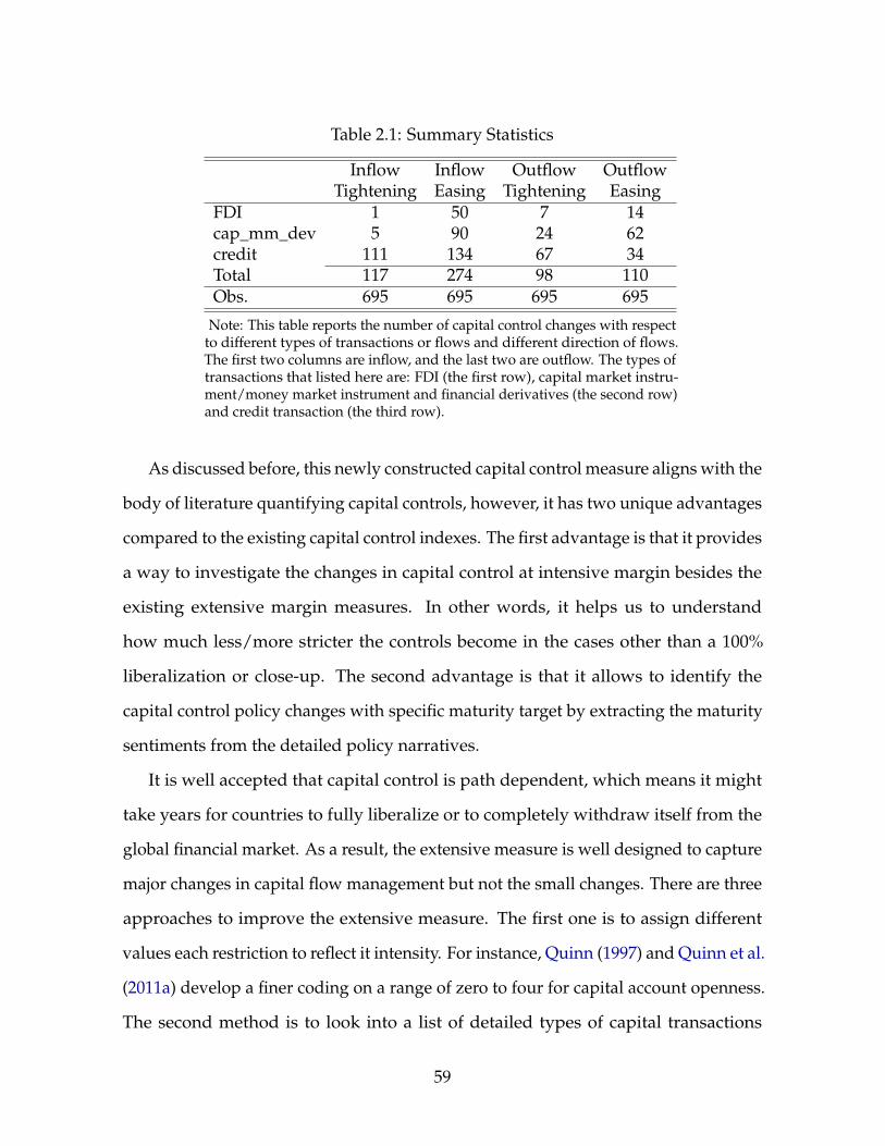
Table 2.1: Summary Statistics

Inflow Inflow Outflow OutflowTightening Easing Tightening Easing

FDI 1 50 7 14cap_mm_dev 5 90 24 62credit 111 134 67 34Total 117 274 98 110Obs. 695 695 695 695

Note: This table reports the number of capital control changes with respectto different types of transactions or flows and different direction of flows.The first two columns are inflow, and the last two are outflow. The types oftransactions that listed here are: FDI (the first row), capital market instru-ment/money market instrument and financial derivatives (the second row)and credit transaction (the third row).

As discussed before, this newly constructed capital control measure aligns with the

body of literature quantifying capital controls, however, it has two unique advantages

compared to the existing capital control indexes. The first advantage is that it provides

a way to investigate the changes in capital control at intensive margin besides the

existing extensive margin measures. In other words, it helps us to understand

how much less/more stricter the controls become in the cases other than a 100%

liberalization or close-up. The second advantage is that it allows to identify the

capital control policy changes with specific maturity target by extracting the maturity

sentiments from the detailed policy narratives.

It is well accepted that capital control is path dependent, which means it might

take years for countries to fully liberalize or to completely withdraw itself from the

global financial market. As a result, the extensive measure is well designed to capture

major changes in capital flow management but not the small changes. There are three

approaches to improve the extensive measure. The first one is to assign different

values each restriction to reflect it intensity. For instance, Quinn (1997) and Quinn et al.

(2011a) develop a finer coding on a range of zero to four for capital account openness.

The second method is to look into a list of detailed types of capital transactions

59

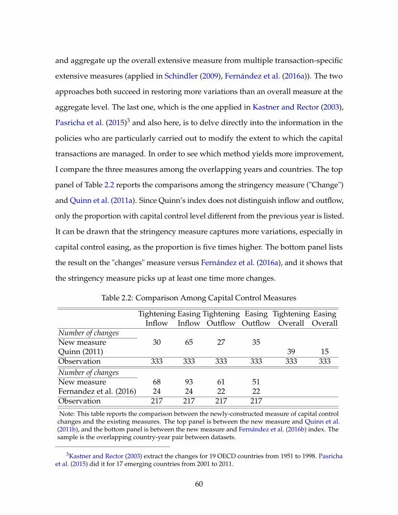
and aggregate up the overall extensive measure from multiple transaction-specific

extensive measures (applied in Schindler (2009), Fernández et al. (2016a)). The two

approaches both succeed in restoring more variations than an overall measure at the

aggregate level. The last one, which is the one applied in Kastner and Rector (2003),

Pasricha et al. (2015)3 and also here, is to delve directly into the information in the

policies who are particularly carried out to modify the extent to which the capital

transactions are managed. In order to see which method yields more improvement,

I compare the three measures among the overlapping years and countries. The top

panel of Table 2.2 reports the comparisons among the stringency measure ("Change")

and Quinn et al. (2011a). Since Quinn’s index does not distinguish inflow and outflow,

only the proportion with capital control level different from the previous year is listed.

It can be drawn that the stringency measure captures more variations, especially in

capital control easing, as the proportion is five times higher. The bottom panel lists

the result on the "changes" measure versus Fernández et al. (2016a), and it shows that

the stringency measure picks up at least one time more changes.

Table 2.2: Comparison Among Capital Control Measures

Tightening Easing Tightening Easing Tightening EasingInflow Inflow Outflow Outflow Overall Overall

Number of changesNew measure 30 65 27 35Quinn (2011) 39 15Observation 333 333 333 333 333 333Number of changesNew measure 68 93 61 51Fernandez et al. (2016) 24 24 22 22Observation 217 217 217 217

Note: This table reports the comparison between the newly-constructed measure of capital controlchanges and the existing measures. The top panel is between the new measure and Quinn et al.(2011b), and the bottom panel is between the new measure and Fernández et al. (2016b) index. Thesample is the overlapping country-year pair between datasets.

3Kastner and Rector (2003) extract the changes for 19 OECD countries from 1951 to 1998. Pasrichaet al. (2015) did it for 17 emerging countries from 2001 to 2011.

60

Besides picking up more variations, the "changes" measure also provides a new

perspective – maturity targeting for examining capital controls. Although policies

generally referring different types of capital transactions abound, for instance, "A new

foreign investment law was adopted, which simplified administrative procedures

for the establishment and taxation of new joint ventures" (Poland, July 4th 1991) for

FDI, and "The acquisition of stocks in resident credit institutions by nonresidents no

longer required CBR approval" (Russia, Dec. 29th 2006) for equity transaction, there

is a significant portion of policies particularly targeting maturities. For instance, "The

minimum mandatory reserve requirement was increased to 30% for deposits in local

currency with maturity of less than 30 days, ... and the minimum mandatory reserve

requirement for foreign currency deposits was reduced to 4% from 10% for maturities

more than 180 days." (Uruguay, Sept. 2nd, 2002), which indicates the mandate to curb

short-term transaction but promote long-term transaction4. This type of information

provides a new angle to investigate the maturity target of capital control policy and

assess its role in adjusting the composition of the cross-border capital flows besides

the level.

In sum, this newly constructed data shares the merits of the existing measures

which distinguish the controls with respect to different directions of and types of

capital flows. Furthermore, it fits better for the purpose of analyzing the capital

control changes in financial crisis because of its fine measure in the stringency of

capital controls, precise information on the maturity target and its full coverage of

the financial crisis periods.

4More information can be found in Appendix about extracting the maturity target.

61

2.3 Economy Fluctuations in Financial Crises

Before delving into the dynamics of capital control changes in financial crisis, it might

be useful to lay out the context of financial crisis per se. Laeven and Valencia (2013)

define financial crisis as the periods with “significant signs of financial distress in the

banking system (as indicated by significant bank runs, losses in the banking system,

and/or bank liquidations)” and “significant banking policy intervention measures in

response to significant losses in the banking system”. Within the 139 financial crises,

there are 28 in advanced countries, 61 in emerging countries and 50 in developing

countries. A typical example of financial crisis in advanced countries is the 2007 crisis

in the U.S., and a typical example for emerging and developing countries is the 1997

Asian crisis.

To see the financial stress and output loss in financial crisis, in the left-hand chart

of Figure 2.1, I plot the output gap and credit-to-gdp ratio gap (the cyclical component

of credit-to-gdp ratio) in a five-year window around the starting year of financial

crisis5. Compared to pre-crisis, there is over 5% output loss in after two years of the

onset of financial crisis and accumulatively 10% output loss over the crisis period.

On the credit side, in the run-up of crisis, there is a rapid growth in private credit,

however, the credit boom is drastically cooled down once the crisis hits. Two years

after the start of financial crisis, the credit-to-gdp ratio is 4% lower than the highest

level.

5Output gap is calculated as the cyclical component of the logarithm of real GDP with quadraticdetrending, and credit-to-gdp ratio gap is calculated as the cyclical component of its level withquadratic detrending. Both real GDP and Domestic credit to private sector as % of GDP are from WDIdataset of the World Bank.

62

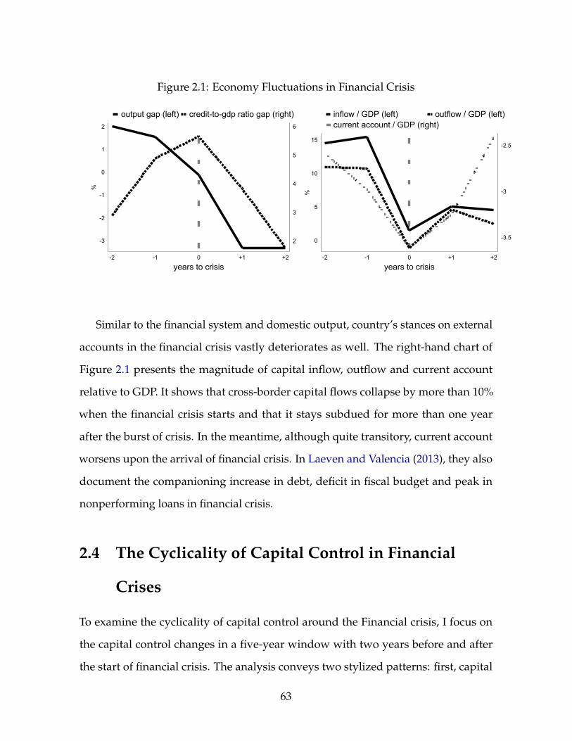
Figure 2.1: Economy Fluctuations in Financial Crisis

2

3

4

5

6

-3

-2

-1

0

1

2

%

-2 -1 0 +1 +2

years to crisis

output gap (left) credit-to-gdp ratio gap (right)

-3.5

-3

-2.5

0

5

10

15

%

-2 -1 0 +1 +2

years to crisis

inflow / GDP (left) outflow / GDP (left)current account / GDP (right)

Similar to the financial system and domestic output, country’s stances on external

accounts in the financial crisis vastly deteriorates as well. The right-hand chart of

Figure 2.1 presents the magnitude of capital inflow, outflow and current account

relative to GDP. It shows that cross-border capital flows collapse by more than 10%

when the financial crisis starts and that it stays subdued for more than one year

after the burst of crisis. In the meantime, although quite transitory, current account

worsens upon the arrival of financial crisis. In Laeven and Valencia (2013), they also

document the companioning increase in debt, deficit in fiscal budget and peak in

nonperforming loans in financial crisis.

2.4 The Cyclicality of Capital Control in Financial

Crises

To examine the cyclicality of capital control around the Financial crisis, I focus on

the capital control changes in a five-year window with two years before and after

the start of financial crisis. The analysis conveys two stylized patterns: first, capital

63

control shows strong procyclicality as no significant changes happen until the start

of financial crisis (procyclicality); second, not only outflow but also inflow are more

constrained once financial crisis begins (dual tightening).

Figure 2.2 presents a panel of charts that characterize the procyclicality and the dual

tightening features of capital control cyclicality. The first chart in the top panel shows

the proportion of crises with capital control tightening at each point in the five-year

financial crisis window. Taking two years prior to the crisis as the initial state, we can

observe that about 3% of the 139 financial crisis periods experience capital control

tightening, and the proportion remains relative stable one year after. However, when

financial crisis hits the economy, there is a remarkable spike in both the inflow control

and outflow control as 12% countries impose tighter constraints on inflow and the

share goes even further to 15% for outflow. As fast as its increase, the tightening fades

out rapidly and it falls down to the pre-crisis level after two years.

Besides the proportion of the crises with capital control tightening, an alternative

measure of capital control tightening is the average number of tightening policies

at each time point. Unlike the proportion measure which represents how likely

capital control is tightened in a financial crisis window, the average number of policy

provides information about to what extent additional capital flow constraints are

employed. The second chart of the top panel in Figure 2.2 shows the result, from

which we can observe a strong comovement of the inflow control and outflow control

and that both of them show a similar inverse-V shape to the proportion measure.

Starting from two-year before crisis, the average number of capital control tightening

is about 0.1, which means on average about one capital control tightening happens

for every ten countries. In the run-up of crisis, there is still no significant tightening.

However, upon the arrival of financial crisis, the average number of tightening

policies jumps to one per three countries. After the start of the financial crisis, the

64

tightening shifts to a declining trend and goes back to the initial level in two years.

The results of proportion and average number based on capital control tightening

provide strong evidence for procyclicality and the dual tightening, but there could be

simultaneous capital control easing offsetting the tightening. To address this concern,

I construct the net average number of capital control tightening policies by subtracting

the number of capital control easing out from tightening to check whether the patterns

still stand. The first chart in the bottom panel of Figure 2.2 presents the result. It is

true that the easing policies carried out at the same time as tightening cancel out a

small amount of tightening policies, yet the net average numbers of policies of both

inflow and outflow maintain the procyclicality. This also indicates that capital control

easing in the financial crisis is not as procyclical as tightening, otherwise, it will be

able to neutralize or even overturn the procyclicality of tightening.

The net measure of capital control tightening has the merit of taking the easing

counterpart into consideration, yet an implicit assumption in the measure construc-

tion is that one tightening policy can be fully offset by one easing policy. This suffers

from the potential shortcoming of neglecting the heterogeneity among policies. For

instance, in 2007, during the financial crisis, Slovenia passed the regulation of credit

inflow easing "The required reserve ratios for deposits in foreign currency and in

euros were unified at 2% for deposits with a maturity up to two years and zero for

longer maturities." which indicates a credit inflow easing (for the longer maturities),

while in the same year there was a capital and money market instrument regulation

stating that "the issuance of capital and money market instruments by residents in the

EU and nonresidents in Slovenia became subject to authorization.". In the previous

net capital control tightening measure, these two policies are equally weighted (the

same as the majority of existing capital control measures) which leads to a net value

of zero. However, the two policies target different types of flows, and the magnitude

65

of them may be too different to make the impact of the two policies comparable. One

possible adjustment is to use the lagged value of type-specific flows as weight to each

capital control policy, and its idea is to proxy the impact of the policy by the pre-policy

level of the target flow. Although imperfect, as the target flow reflects only one aspect

of the intensity of the capital control policy, it would still provide some sense of the

evolution of capital control if the intensity of each policy is partially addressed. The

last chart in Figure 2.2 plots the time series of the weighted net average number of

capital control tightening6. Although the pattern is nosier than the previous three, it

still generates that capital control inflow and outflow are significantly tightened when

the financial crisis hits the economy. There is certain amount of ongoing fluctuation

after the beginning of financial crisis, but none of them is significant.

6The historical inflow and outflow data with respect to different flows is from BOP dataset(IMF). The flow associated with "capital market instrument/money market instrument/financialderivatives" is the sum of portfolio investment and financial derivatives. The credit transaction flow isthe subcategory of deposit and loan to commercial banks within the other flows category. Becausethe break-down of "other flows" is very patchy, the data only allows constructing the weight-adjustedmeasure for 41 financial crisis periods after 1988.

66

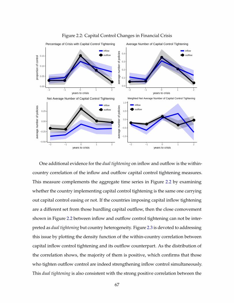
Figure 2.2: Capital Control Changes in Financial Crisis

● ●

●

●

●

0.00

0.05

0.10

0.15

−2 −1 0 1 2

years to crisis

prop

ortio

n of

con

trol ●

inflow

outflow

Percentage of Crisis with Capital Control Tightening

● ●

●

●

●0.0

0.1

0.2

0.3

0.4

−2 −1 0 1 2

years to crisis

aver

age

num

ber

of p

olic

ies

●

inflow

outflow

Average Number of Capital Control Tightening

● ●

●

● ●

−0.50

−0.25

0.00

0.25

−2 −1 0 1 2

years to crisis

aver

age

num

ber

of p

olic

ies

●

inflow

outflow

Net Average Number of Capital Control Tightening

● ●

●

●

●

−1.0

−0.5

0.0

0.5

1.0

−2 −1 0 1 2

years to crisis

aver

age

num

ber

of p

olic

ies

●

inflow

outflow

Weighted Net Average Number of Capital Control Tightening

One additional evidence for the dual tightening on inflow and outflow is the within-

country correlation of the inflow and outflow capital control tightening measures.

This measure complements the aggregate time series in Figure 2.2 by examining

whether the country implementing capital control tightening is the same one carrying

out capital control easing or not. If the countries imposing capital inflow tightening

are a different set from those hurdling capital outflow, then the close comovement

shown in Figure 2.2 between inflow and outflow control tightening can not be inter-

preted as dual tightening but country heterogeneity. Figure 2.3 is devoted to addressing

this issue by plotting the density function of the within-country correlation between

capital inflow control tightening and its outflow counterpart. As the distribution of

the correlation shows, the majority of them is positive, which confirms that those

who tighten outflow control are indeed strengthening inflow control simultaneously.

This dual tightening is also consistent with the strong positive correlation between the

67

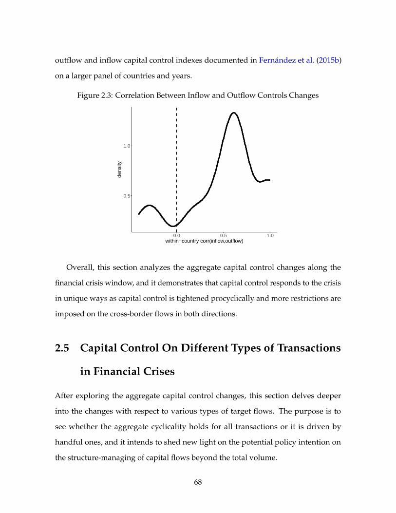
outflow and inflow capital control indexes documented in Fernández et al. (2015b)

on a larger panel of countries and years.

Figure 2.3: Correlation Between Inflow and Outflow Controls Changes

0.5

1.0

0.0 0.5 1.0within−country corr(inflow,outflow)

dens

ity

Overall, this section analyzes the aggregate capital control changes along the

financial crisis window, and it demonstrates that capital control responds to the crisis

in unique ways as capital control is tightened procyclically and more restrictions are

imposed on the cross-border flows in both directions.

2.5 Capital Control On Different Types of Transactions

in Financial Crises

After exploring the aggregate capital control changes, this section delves deeper

into the changes with respect to various types of target flows. The purpose is to

see whether the aggregate cyclicality holds for all transactions or it is driven by

handful ones, and it intends to shed new light on the potential policy intention on

the structure-managing of capital flows beyond the total volume.

68

Figure 2.4 presents evidence of a strong asymmetry between inflow and outflow

capital control changes with flows break-down. On one hand, the inflow control pol-

icy exclusively focuses on credit transaction with barely any changes on the rest two;

on the other, the outflow control policy is applied to a broader range of transactions

including not only credit transaction but also capital market instrument/money mar-

ket instrument/financial derivatives. To provide detailed evidence, in the top panel

of Figure 2.4, I plot the average number of capital inflow control policies with respect

to different types of transactions in both gross and net measure (on the left-hand

side and on the right-hand side, respectively). The charts show remarkably different

patterns between credit transaction and the rest two. The capital control policy on

credit transaction almost triples when the financial crisis hits the economy, while the

policies concerning the other two remain highly stable from the run-up of crisis to the

burst of crisis and to the span of crisis.

However, this sharp contrast among different types of transactions in the inflow

controls is much less prominent in the case of outflow control policies. In the bottom

panel of Figure 2.4, I show the evolution for how the outflow control policies respond

to financial crisis. It can be observed that credit transaction is not the sole center of

policy attention anymore, and control on capital market instrument/money market

instrument/financial derivatives is strengthened as well.

69

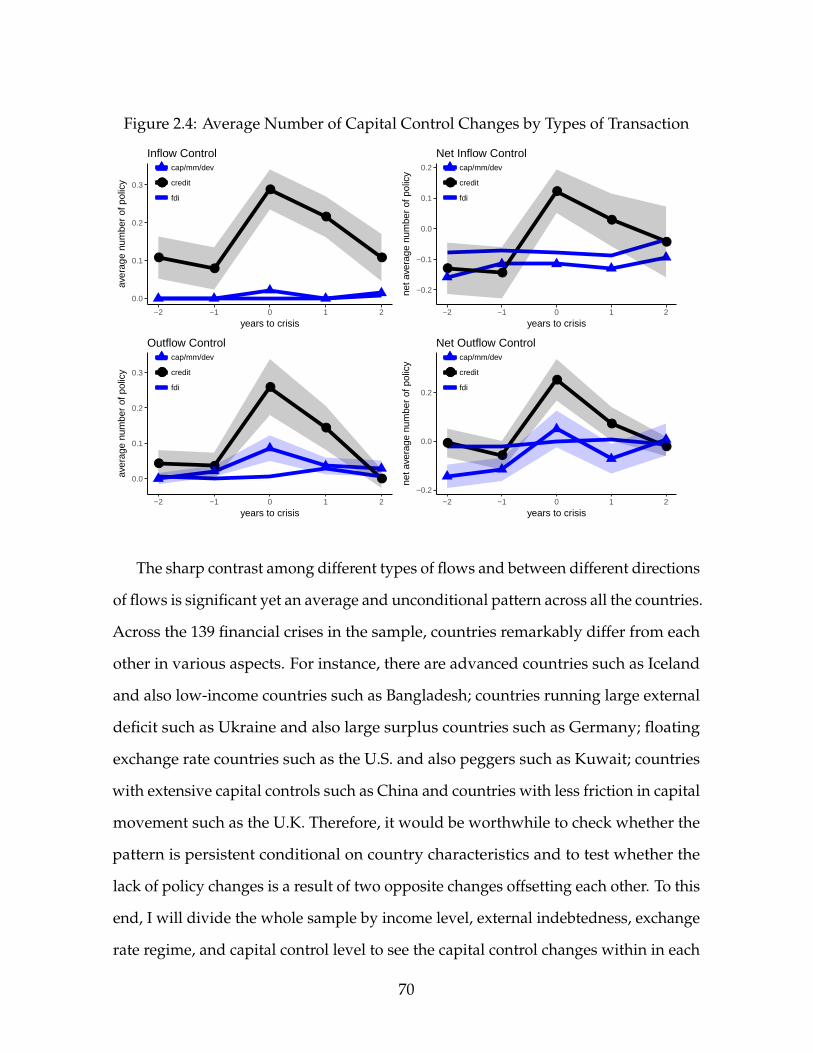
Figure 2.4: Average Number of Capital Control Changes by Types of Transaction

●●

●

●

●

0.0

0.1

0.2

0.3

−2 −1 0 1 2

years to crisis

aver

age

num

ber

of p

olic

y ●●

cap/mm/dev

credit

fdi

Inflow Control

● ●

●

●

●

−0.2

−0.1

0.0

0.1

0.2

−2 −1 0 1 2

years to crisis

net a

vera

ge n

umbe

r of

pol

icy

●●

cap/mm/dev

credit

fdi

Net Inflow Control

● ●

●

●

●0.0

0.1

0.2

0.3

−2 −1 0 1 2

years to crisis

aver

age

num

ber

of p

olic

y ●●

cap/mm/dev

credit

fdi

Outflow Control

●●

●

●

●

−0.2

0.0

0.2

−2 −1 0 1 2

years to crisis

net a

vera

ge n

umbe

r of

pol

icy

●●

cap/mm/dev

credit

fdi

Net Outflow Control

The sharp contrast among different types of flows and between different directions

of flows is significant yet an average and unconditional pattern across all the countries.

Across the 139 financial crises in the sample, countries remarkably differ from each

other in various aspects. For instance, there are advanced countries such as Iceland

and also low-income countries such as Bangladesh; countries running large external

deficit such as Ukraine and also large surplus countries such as Germany; floating

exchange rate countries such as the U.S. and also peggers such as Kuwait; countries

with extensive capital controls such as China and countries with less friction in capital

movement such as the U.K. Therefore, it would be worthwhile to check whether the

pattern is persistent conditional on country characteristics and to test whether the

lack of policy changes is a result of two opposite changes offsetting each other. To this

end, I will divide the whole sample by income level, external indebtedness, exchange

rate regime, and capital control level to see the capital control changes within in each

70

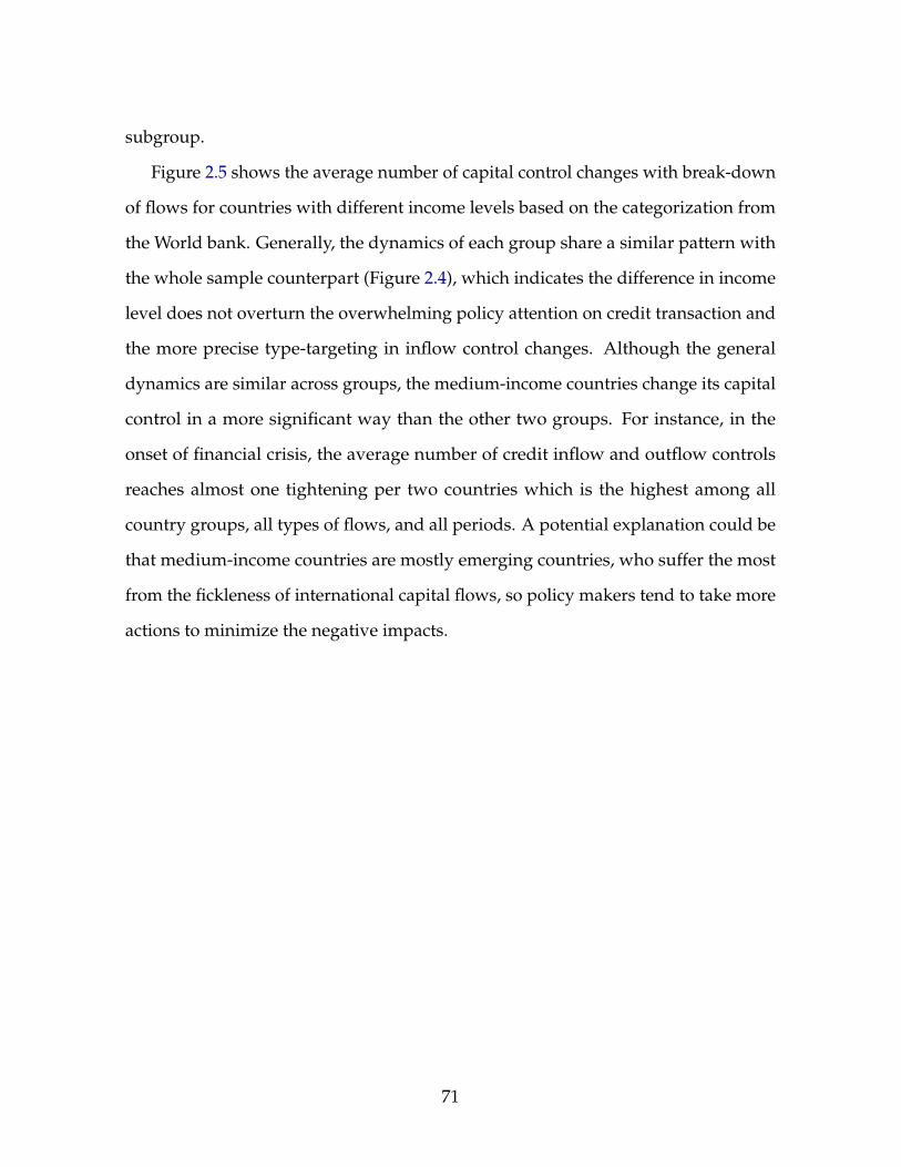
subgroup.

Figure 2.5 shows the average number of capital control changes with break-down

of flows for countries with different income levels based on the categorization from

the World bank. Generally, the dynamics of each group share a similar pattern with

the whole sample counterpart (Figure 2.4), which indicates the difference in income

level does not overturn the overwhelming policy attention on credit transaction and

the more precise type-targeting in inflow control changes. Although the general

dynamics are similar across groups, the medium-income countries change its capital

control in a more significant way than the other two groups. For instance, in the

onset of financial crisis, the average number of credit inflow and outflow controls

reaches almost one tightening per two countries which is the highest among all

country groups, all types of flows, and all periods. A potential explanation could be

that medium-income countries are mostly emerging countries, who suffer the most

from the fickleness of international capital flows, so policy makers tend to take more

actions to minimize the negative impacts.

71

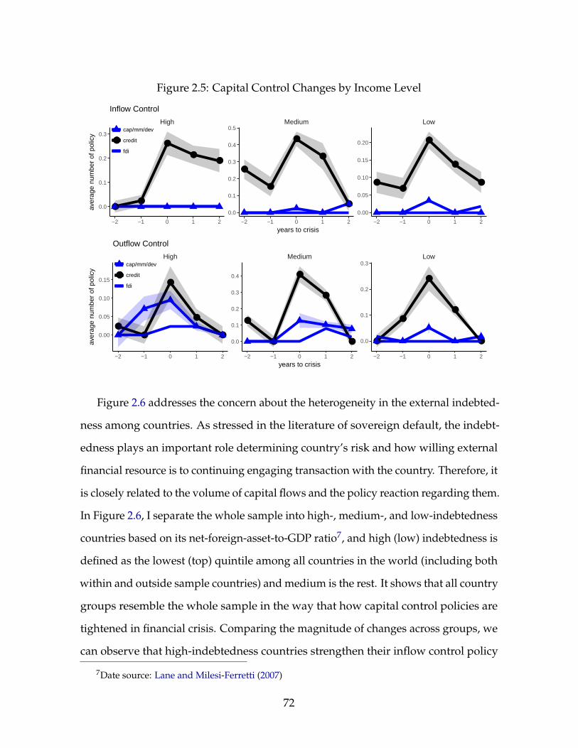
Figure 2.5: Capital Control Changes by Income Level

●●

●

●●

●

●

●

●

●

●●

●

●

●

High Medium Low

−2 −1 0 1 2 −2 −1 0 1 2 −2 −1 0 1 2

0.00

0.05

0.10

0.15

0.20

0.0

0.1

0.2

0.3

0.4

0.5

0.0

0.1

0.2

0.3

years to crisis

aver

age

num

ber

of p

olic

y

●●

cap/mm/dev

credit

fdi

Inflow Control

●●

●

●

●

●

●

●

●

● ●

●

●

●

●

High Medium Low

−2 −1 0 1 2 −2 −1 0 1 2 −2 −1 0 1 2

0.0

0.1

0.2

0.3

0.0

0.1

0.2

0.3

0.4

0.00

0.05

0.10

0.15

years to crisis

aver

age

num

ber

of p

olic

y

●●

cap/mm/dev

credit

fdi

Outflow Control

Figure 2.6 addresses the concern about the heterogeneity in the external indebted-

ness among countries. As stressed in the literature of sovereign default, the indebt-

edness plays an important role determining country’s risk and how willing external

financial resource is to continuing engaging transaction with the country. Therefore, it

is closely related to the volume of capital flows and the policy reaction regarding them.

In Figure 2.6, I separate the whole sample into high-, medium-, and low-indebtedness

countries based on its net-foreign-asset-to-GDP ratio7, and high (low) indebtedness is

defined as the lowest (top) quintile among all countries in the world (including both

within and outside sample countries) and medium is the rest. It shows that all country

groups resemble the whole sample in the way that how capital control policies are

tightened in financial crisis. Comparing the magnitude of changes across groups, we

can observe that high-indebtedness countries strengthen their inflow control policy

7Date source: Lane and Milesi-Ferretti (2007)

72

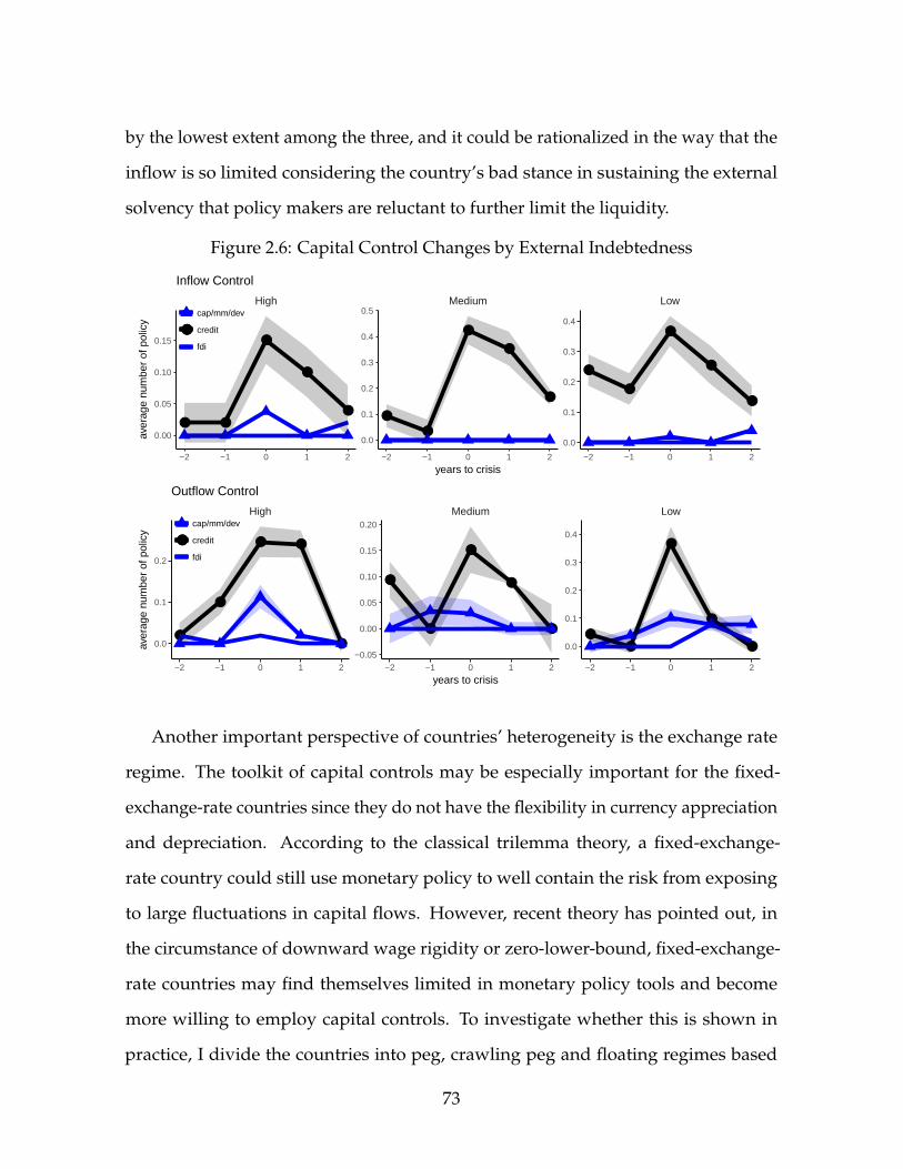
by the lowest extent among the three, and it could be rationalized in the way that the

inflow is so limited considering the country’s bad stance in sustaining the external

solvency that policy makers are reluctant to further limit the liquidity.

Figure 2.6: Capital Control Changes by External Indebtedness

● ●

●

●

● ●

●

●

●

●

●

●

●

●

●

High Medium Low

−2 −1 0 1 2 −2 −1 0 1 2 −2 −1 0 1 2

0.0

0.1

0.2

0.3

0.4

0.0

0.1

0.2

0.3

0.4

0.5

0.00

0.05

0.10

0.15

years to crisis

aver

age

num

ber

of p

olic

y

●●

cap/mm/dev

credit

fdi

Inflow Control

●

●

● ●

●

●

●

●

●

● ●●

●

●

●

High Medium Low

−2 −1 0 1 2 −2 −1 0 1 2 −2 −1 0 1 2

0.0

0.1

0.2

0.3

0.4

−0.05

0.00

0.05

0.10

0.15

0.20

0.0

0.1

0.2

years to crisis

aver

age

num

ber

of p

olic

y

●●

cap/mm/dev

credit

fdi

Outflow Control

Another important perspective of countries’ heterogeneity is the exchange rate

regime. The toolkit of capital controls may be especially important for the fixed-

exchange-rate countries since they do not have the flexibility in currency appreciation

and depreciation. According to the classical trilemma theory, a fixed-exchange-

rate country could still use monetary policy to well contain the risk from exposing

to large fluctuations in capital flows. However, recent theory has pointed out, in

the circumstance of downward wage rigidity or zero-lower-bound, fixed-exchange-

rate countries may find themselves limited in monetary policy tools and become

more willing to employ capital controls. To investigate whether this is shown in

practice, I divide the countries into peg, crawling peg and floating regimes based

73

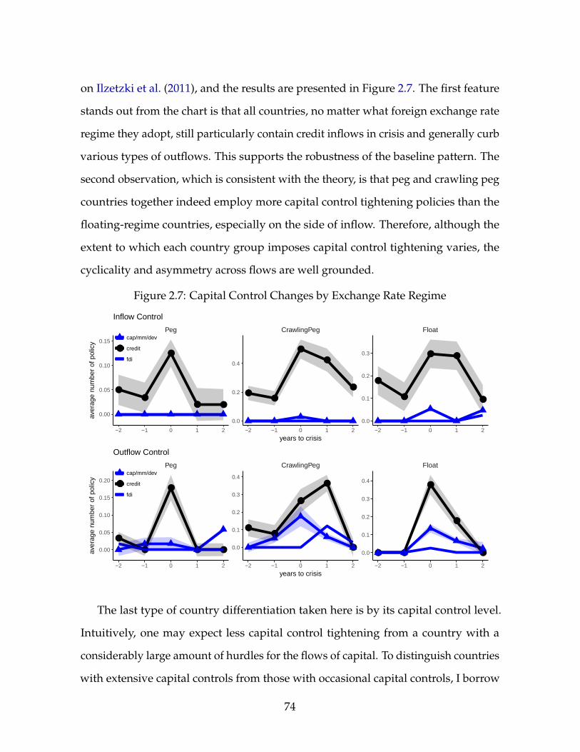
on Ilzetzki et al. (2011), and the results are presented in Figure 2.7. The first feature

stands out from the chart is that all countries, no matter what foreign exchange rate

regime they adopt, still particularly contain credit inflows in crisis and generally curb

various types of outflows. This supports the robustness of the baseline pattern. The

second observation, which is consistent with the theory, is that peg and crawling peg

countries together indeed employ more capital control tightening policies than the

floating-regime countries, especially on the side of inflow. Therefore, although the

extent to which each country group imposes capital control tightening varies, the

cyclicality and asymmetry across flows are well grounded.

Figure 2.7: Capital Control Changes by Exchange Rate Regime

●●

●

● ●

●●

●

●

●●

●

● ●

●

Peg CrawlingPeg Float

−2 −1 0 1 2 −2 −1 0 1 2 −2 −1 0 1 2

0.0

0.1

0.2

0.3

0.0

0.2

0.4

0.00

0.05

0.10

0.15

years to crisis

aver

age

num

ber

of p

olic

y

●●

cap/mm/dev

credit

fdi

Inflow Control

●

●

●

● ●

●●

●

●

●● ●

●

●

●

Peg CrawlingPeg Float

−2 −1 0 1 2 −2 −1 0 1 2 −2 −1 0 1 2

0.0

0.1

0.2

0.3

0.4

0.0

0.1

0.2

0.3

0.4

0.00

0.05

0.10

0.15

0.20

years to crisis

aver

age

num

ber

of p

olic

y

●●

cap/mm/dev

credit

fdi

Outflow Control

The last type of country differentiation taken here is by its capital control level.

Intuitively, one may expect less capital control tightening from a country with a

considerably large amount of hurdles for the flows of capital. To distinguish countries

with extensive capital controls from those with occasional capital controls, I borrow

74

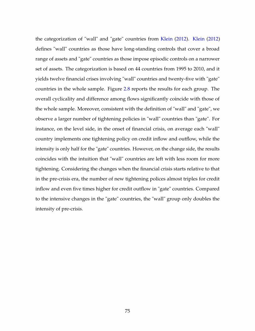
the categorization of "wall" and "gate" countries from Klein (2012). Klein (2012)

defines "wall" countries as those have long-standing controls that cover a broad

range of assets and "gate" countries as those impose episodic controls on a narrower

set of assets. The categorization is based on 44 countries from 1995 to 2010, and it

yields twelve financial crises involving "wall" countries and twenty-five with "gate"

countries in the whole sample. Figure 2.8 reports the results for each group. The

overall cyclicality and difference among flows significantly coincide with those of

the whole sample. Moreover, consistent with the definition of "wall" and "gate", we

observe a larger number of tightening policies in "wall" countries than "gate". For

instance, on the level side, in the onset of financial crisis, on average each "wall"

country implements one tightening policy on credit inflow and outflow, while the

intensity is only half for the "gate" countries. However, on the change side, the results

coincides with the intuition that "wall" countries are left with less room for more

tightening. Considering the changes when the financial crisis starts relative to that

in the pre-crisis era, the number of new tightening polices almost triples for credit

inflow and even five times higher for credit outflow in "gate" countries. Compared

to the intensive changes in the "gate" countries, the "wall" group only doubles the

intensity of pre-crisis.

75

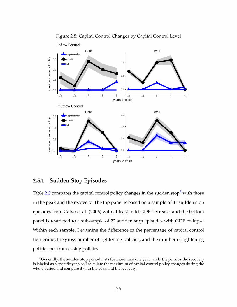
Figure 2.8: Capital Control Changes by Capital Control Level

●

●

●

●●

●

●

●●

●

Gate Wall

−2 −1 0 1 2 −2 −1 0 1 2

0.0

0.5

1.0

0.0

0.1

0.2

0.3

years to crisis

aver

age

num

ber

of p

olic

y

●●

cap/mm/dev

credit

fdi

Inflow Control

●●

●

●

●

●

●

●

●

●

Gate Wall

−2 −1 0 1 2 −2 −1 0 1 2

0.0

0.4

0.8

1.2

0.0

0.2

0.4

0.6

years to crisis

aver

age

num

ber

of p

olic

y

●●

cap/mm/dev

credit

fdi

Outflow Control

2.5.1 Sudden Stop Episodes

Table 2.3 compares the capital control policy changes in the sudden stop8 with those

in the peak and the recovery. The top panel is based on a sample of 33 sudden stop

episodes from Calvo et al. (2006) with at least mild GDP decrease, and the bottom

panel is restricted to a subsample of 22 sudden stop episodes with GDP collapse.

Within each sample, I examine the difference in the percentage of capital control

tightening, the gross number of tightening policies, and the number of tightening

policies net from easing policies.

8Generally, the sudden stop period lasts for more than one year while the peak or the recoveryis labeled as a specific year, so I calculate the maximum of capital control policy changes during thewhole period and compare it with the peak and the recovery.

76

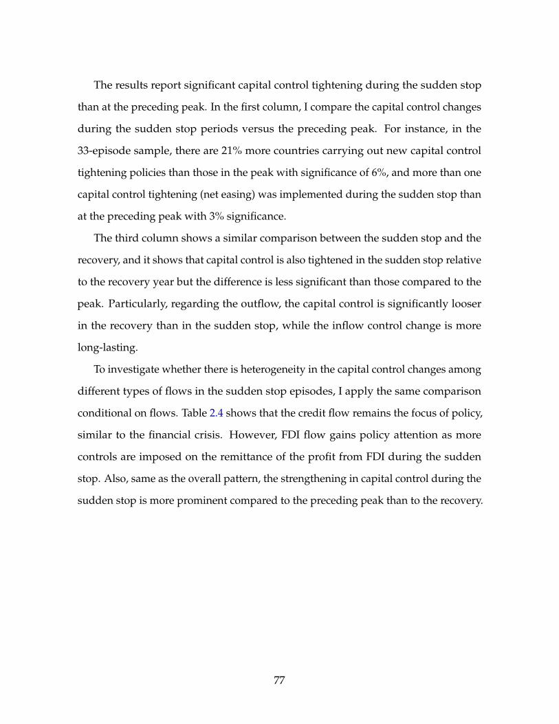
The results report significant capital control tightening during the sudden stop

than at the preceding peak. In the first column, I compare the capital control changes

during the sudden stop periods versus the preceding peak. For instance, in the

33-episode sample, there are 21% more countries carrying out new capital control

tightening policies than those in the peak with significance of 6%, and more than one

capital control tightening (net easing) was implemented during the sudden stop than

at the preceding peak with 3% significance.

The third column shows a similar comparison between the sudden stop and the

recovery, and it shows that capital control is also tightened in the sudden stop relative

to the recovery year but the difference is less significant than those compared to the

peak. Particularly, regarding the outflow, the capital control is significantly looser

in the recovery than in the sudden stop, while the inflow control change is more

long-lasting.

To investigate whether there is heterogeneity in the capital control changes among

different types of flows in the sudden stop episodes, I apply the same comparison

conditional on flows. Table 2.4 shows that the credit flow remains the focus of policy,

similar to the financial crisis. However, FDI flow gains policy attention as more

controls are imposed on the remittance of the profit from FDI during the sudden

stop. Also, same as the overall pattern, the strengthening in capital control during the

sudden stop is more prominent compared to the preceding peak than to the recovery.

77

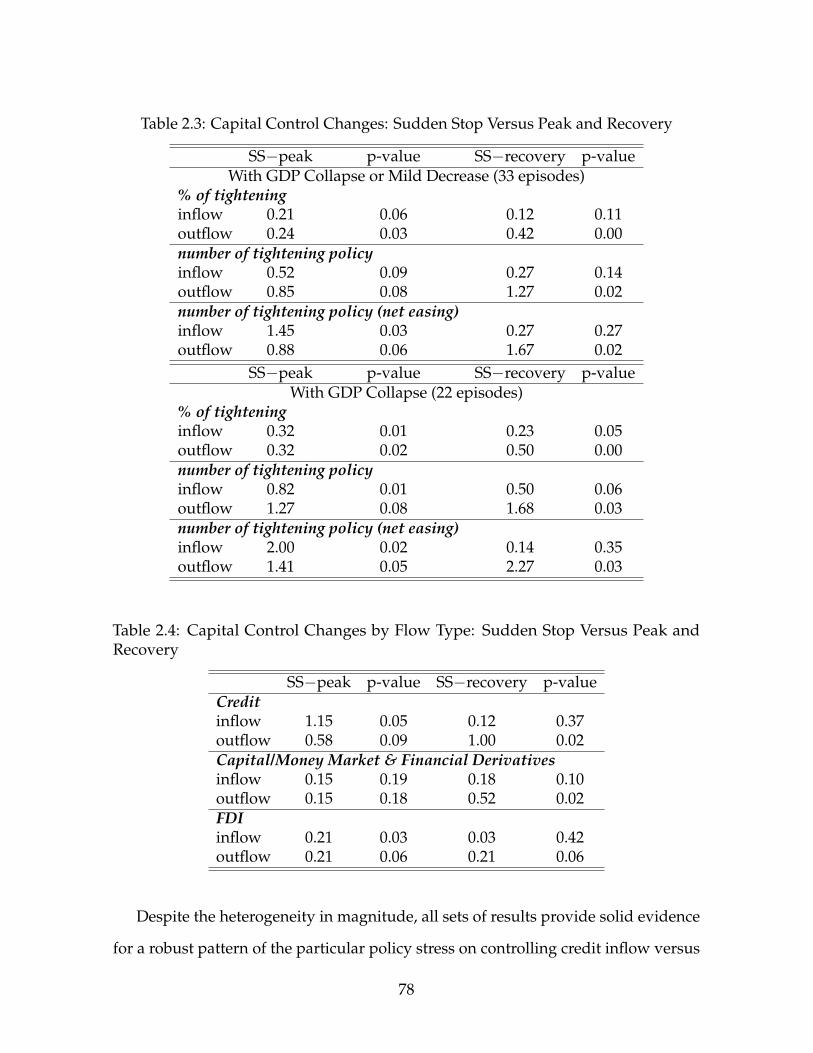
Table 2.3: Capital Control Changes: Sudden Stop Versus Peak and Recovery

SS−peak p-value SS−recovery p-valueWith GDP Collapse or Mild Decrease (33 episodes)

% of tighteninginflow 0.21 0.06 0.12 0.11outflow 0.24 0.03 0.42 0.00number of tightening policyinflow 0.52 0.09 0.27 0.14outflow 0.85 0.08 1.27 0.02number of tightening policy (net easing)inflow 1.45 0.03 0.27 0.27outflow 0.88 0.06 1.67 0.02

SS−peak p-value SS−recovery p-valueWith GDP Collapse (22 episodes)

% of tighteninginflow 0.32 0.01 0.23 0.05outflow 0.32 0.02 0.50 0.00number of tightening policyinflow 0.82 0.01 0.50 0.06outflow 1.27 0.08 1.68 0.03number of tightening policy (net easing)inflow 2.00 0.02 0.14 0.35outflow 1.41 0.05 2.27 0.03

Table 2.4: Capital Control Changes by Flow Type: Sudden Stop Versus Peak andRecovery

SS−peak p-value SS−recovery p-valueCreditinflow 1.15 0.05 0.12 0.37outflow 0.58 0.09 1.00 0.02Capital/Money Market & Financial Derivativesinflow 0.15 0.19 0.18 0.10outflow 0.15 0.18 0.52 0.02FDIinflow 0.21 0.03 0.03 0.42outflow 0.21 0.06 0.21 0.06

Despite the heterogeneity in magnitude, all sets of results provide solid evidence

for a robust pattern of the particular policy stress on controlling credit inflow versus

78

the general tightening on a wide range of transactions. The pattern holds well across

countries differing in development status and policy stances. It naturally leads to

the question, what contributes to the pattern? Especially, what distinguishes credit

inflow from the others?

One hypothesis would be credit inflow is more volatile than the rest. However, the

argument lacks solid grounds from the literature. For instance, Bluedorn et al. (2013)

use a large panel covering 150 countries with more than three decades to analyze

the dynamics of capital flows, and they find there is little significant difference in

volatility across portfolio and bank-related flows. Eichengreen et al. (2017) construct

a quarterly sample of 34 emerging countries and show that both portfolio debt and

bank-intermediated flows remain the most volatile.

Another hypothesis is that bank is most related to credit transaction among all

cross-border capital flows and that policy may concentrate on credit flows in order to

resolve the issue of financial system who is at the center of financial crisis. However,

although there is a considerable amount of capital control changes regarding the

reserve ratio, the minimal maturity, and transaction tax of banks, there are policies

regulating the overall private borrowing as well. For instance, Iceland carried out new

policy in 2009 to limit the external borrowing in general instead of specific to those

channeled by financial system. Moreover, this hypothesis would indicate that any

cross-border transactions intermediated by banks will be subject to regulation, yet

this is not the case. As will be demonstrated in the next section, the policy attention

on credit transaction does not aim at constraining all bank’s transactions as a whole.

Different from the previous hypotheses, here I propose to a new angle to investi-

gate the asymmetry between inflow and outflow controls: the maturity targeting. The

results (detailed in the next section) show that the asymmetry in target flows is closely

associated with asymmetry in target maturities as short-term inflow is particularly

79

constrained while less emphasis on maturity is found on outflow controls.

2.6 The Maturity Targeting of Capital Controls

In order to analyze the maturity targeting of capital control policies, the first step is

to distinguish which policies contain specific maturity target (labeled as "maturity-

related policy"). In the second step, for each of the maturity-related policy, differen-

tiate whether the policy intention is to target short-term flows (or increase average

maturity) or long-term flows (or decrease average maturity)9. Corresponding to

the two measures, there are two perspectives worth looking into for examining the

dynamics of maturity targeting of capital control policies: the proportion of maturity-

related policies relative to the total changes, and the proportion of short-term-targeted

policies relative to total changes. The former tells whether the capital control becomes

more particular or more general in terms of targeting flow’s maturity, and the latter

further pins down what is the targeted maturity if there is one.

Figure 2.9 provides strong evidence for the increasing maturity attention for inflow

control changes in financial crisis and the dominant emphasis on short-term inflow.

The left-hand chart plots the proportion of maturity-related policy to the total number

of policy changes for inflow and outflow tightening, respectively, and we can observe

that the maturity-related policy moves in a completely opposite way between inflow

tightening and outflow tightening. For instance, as the economy approaches the crisis,

there are more and more maturity-related inflow control policies but fewer and fewer

outflow counterpart. When the financial crisis arrives, the maturity-related policy

accounts for about half of the total inflow tightening, which doubles the pre-crisis

level. In the meantime, the maturity-related policy only constitutes 10% of the total

outflow tightening policy, which is less than one quarter of the pre-crisis level. The

9Detailed procedure can be found in Appendix.

80

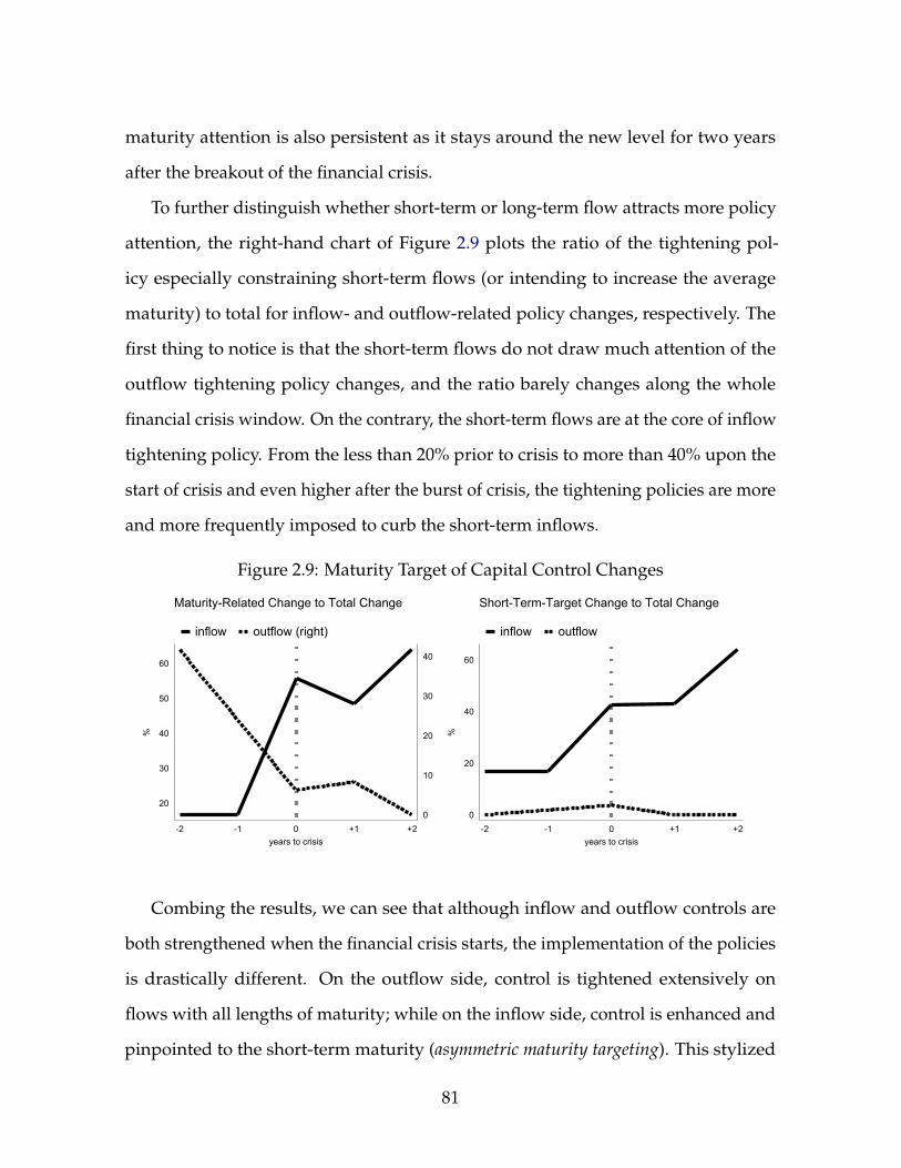
maturity attention is also persistent as it stays around the new level for two years

after the breakout of the financial crisis.

To further distinguish whether short-term or long-term flow attracts more policy

attention, the right-hand chart of Figure 2.9 plots the ratio of the tightening pol-

icy especially constraining short-term flows (or intending to increase the average

maturity) to total for inflow- and outflow-related policy changes, respectively. The

first thing to notice is that the short-term flows do not draw much attention of the

outflow tightening policy changes, and the ratio barely changes along the whole

financial crisis window. On the contrary, the short-term flows are at the core of inflow

tightening policy. From the less than 20% prior to crisis to more than 40% upon the

start of crisis and even higher after the burst of crisis, the tightening policies are more

and more frequently imposed to curb the short-term inflows.

Figure 2.9: Maturity Target of Capital Control Changes

0

10

20

30

40

20

30

40

50

60

%

-2 -1 0 +1 +2years to crisis

inflow outflow (right)

Maturity-Related Change to Total Change

0

20

40

60

%

-2 -1 0 +1 +2years to crisis

inflow outflow

Short-Term-Target Change to Total Change

Combing the results, we can see that although inflow and outflow controls are

both strengthened when the financial crisis starts, the implementation of the policies

is drastically different. On the outflow side, control is tightened extensively on

flows with all lengths of maturity; while on the inflow side, control is enhanced and

pinpointed to the short-term maturity (asymmetric maturity targeting). This stylized

81

pattern reveals the composition adjusting beyond the volume controlling of the

capital control policy, and it also provides a rationale for the asymmetry in the flow

targeting illustrated in the last section, indicating the maturity characteristics of

different transactions plays an important role in the policy determination.

2.7 Maturity-dependent Reserve Requirements

Exploring the information from the policy statements provides a meaningful way

to examine the potential maturity-targeting mandate in capital inflow controls, yet

essentially it is an indicator measure on whether the policy constrains short-term

inflow or long-term inflow. In order to provide further insights on the extent to which

the short-term capital inflow is more regulated than the long-term, I use the reserve

requirements on different types of deposit from Federico et al. (2014). There are

two advantages of this measure: first, it is continuous which enables the magnitude

comparison; second, for considerable amount of countries, the reserve requirement is

set based on the currency and the type of deposit which helps to distinguish external

borrowing with respect to different maturities. According to the categorization of

deposit, I associate the reserve requirement on foreign currency term deposit as long-

term external borrowing and that on foreign currency demand deposit as short-term

external borrowing.10

Figure 2.10 shows the dynamics of reserve requirements in the financial crisis

periods. The left panel displays the proportion of financial crises in which reserve

requirement increases. Prior to crisis, there are barely any increase in reserve require-

ments, however, once the crisis materializes, in about 40% of crises, policy makers

10Capital inflow could take the form of domestic currency deposit as well, and likewise foreigncurrency deposit could be from domestic fund. Therefore, I check the domestic currency term depositand demand deposit reserve requirement for the same countries and same period as foreign currency,and the domestic currency reserve requirement with respect to different maturity shows a qualitativelysimilar pattern with the foreign counterpart.

82

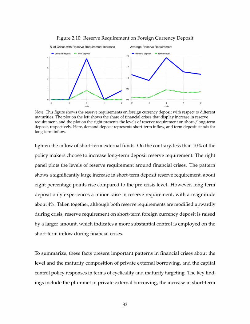
Figure 2.10: Reserve Requirement on Foreign Currency Deposit

0

.1

.2

.3

.4

-2 -1 0 1 2crisis

demand deposit term deposit

% of Crises with Reserve Requirement Increase

.05

.09

.13

.17

.21

-2 -1 0 1 2crisis

demand deposit term deposit

Average Reserve Requirement

Note: This figure shows the reserve requirements on foreign currency deposit with respect to differentmaturities. The plot on the left shows the share of financial crises that display increase in reserverequirement, and the plot on the right presents the levels of reserve requirement on short-/long-termdeposit, respectively. Here, demand deposit represents short-term inflow, and term deposit stands forlong-term inflow.

tighten the inflow of short-term external funds. On the contrary, less than 10% of the

policy makers choose to increase long-term deposit reserve requirement. The right

panel plots the levels of reserve requirement around financial crises. The pattern

shows a significantly large increase in short-term deposit reserve requirement, about

eight percentage points rise compared to the pre-crisis level. However, long-term

deposit only experiences a minor raise in reserve requirement, with a magnitude

about 4%. Taken together, although both reserve requirements are modified upwardly

during crisis, reserve requirement on short-term foreign currency deposit is raised

by a larger amount, which indicates a more substantial control is employed on the

short-term inflow during financial crises.

To summarize, these facts present important patterns in financial crises about the

level and the maturity composition of private external borrowing, and the capital

control policy responses in terms of cyclicality and maturity targeting. The key find-

ings include the plummet in private external borrowing, the increase in short-term

83

borrowing, the capital inflow tightening, and the short-term inflow targeting in tight-

ening policies. Based on these observations, the next section introduces a model of

international borrowing with financial friction which is consistent with these stylized

facts: private agent reduces external borrowing and shift to short-term debt during

crisis, and the optimal capital control policy should tighten capital inflows constraints,

particularly for short-term inflows.

2.8 Conclusion

Along with the rapid pace of global financial integration, more and more attention has

been drawn to the cross-border capital flows for its vast volume and high fickleness

which may deteriorate the receiving country’s financial system and trigger financial

crisis. This paper tends to provide empirical analysis on how countries cope with

fluctuations in cross-border capital flows in financial crisis, in particular, when capital

control polices are imposed, what type of capital control policies are employed, and

in what way they are implemented.

To investigate the evolution of capital control policies in financial crisis, I first

construct a novel capital control stringency measure utilizing the policy changes

documented in the AREAER. It complements the existing capital control indexes

by quantifying the changes in the intensity of capital control, which overcomes the

possible missing variation in the measures based on capital control levels. Besides

sharing the merits of differentiating the capital control policies with respect to differ-

ent directions of flows and different types of transactions with the latest development

in quantifying capital controls (e.g. Schindler (2009), Fernández et al. (2016a)), it

further distinguishes different maturities of target flows, which provides a new angle

to examine the capital control policies.

The newly constructed data reveals three stylized facts about capital control

84

policies in financial crisis. The first one is procyclicality, which is that capital control

policy barely changes until financial crisis starts and that once financial crisis hits

the economy, the controls are strengthened. The second one is dual tightening, which

shows that both inflow and outflow controls are significantly enhanced upon the

arrival of financial crisis. The third one is asymmetric maturity targeting, which refers

to the distinct pattern between inflow control and outflow control regarding the

maturity of the targeted flows. Inflow control changes substantially differ from its

outflow counterpart as the particularly target short-term flows while controls are

generally tightened regardless of the maturity on the side of outflow.

These stylized facts also bring new perspectives to the theoretical literature. For

instance, the existing papers on optimal capital control policy have primarily focused

on the net flow which naturally yields optimal policy as strengthening control on

inflow (outflow) and easing the other. This is opposite to the strong comovement

of the inflow and outflow controls observed in the data. Also, most attention has

been drawn to curbing the level of capital flow, while the asymmetric maturity targeting

shows the maturity structure is also a critical concern of policy.

In an ongoing work, I propose a model with gross capital flows and different

maturities to jointly rationalize the stylized facts. The mechanism works in the

way that in financial crisis, outflow, no matter in what type, imposes downward

pressure on the real exchange rate, therefore the optimal policies aiming at reducing

the depreciation pressure suppress any possible capital flow leaving the country.

However, for inflow, the maturity of external liability matters. It is because short-term

liability bears rollover risk while that long-term liability helps to alleviate fire-sale and

consequently the rollover risk of short-term liability in financial crisis. The private

agent overlooks the social welfare benefit of long-term liability and over-borrows in

short-term. Therefore, the optimal capital inflow control especially targets short-term

85

liability to offset the externality.

So far, I have been focusing on the countries who adjusts capital control policies

in response to financial crisis, however, there is a considerable number of countries

who do not change their cross-border flows management. It would be interesting to

investigate what contributes to this difference. It could be that some countries find

domestic policies such as financial sector regulation is more effective than capital

controls in their cases, or the cost of tightening capital control such as loss of liquidity

is much higher than the benefit, or even the political issue plays an important role in

some countries such as EU members.d These are a few among many worth-pursuing

future works.

86

Chapter 3

Quality of Public Governance and the Capital Structure

of Nations and Firms (with Shang-Jin Wei)

87

3.1 Introduction

The composition of capital flows matters for economic efficiency (for instance, Levchenko

and Mauro (2007), Contessi et al. (2013), Evans and Hnatkovska (2014)) and financial

stability. For example, in the immediate aftermath of the Global Financial Crisis of

2008-2009, countries that rely more on external debt exhibit a stronger liquidity shock

at home than countries that rely more on foreign direct investment, 1 and long-term

debt plays an important role in credit risk and business cycle dynamics.2

In this paper, we study the role of the quality of domestic institutions in determin-

ing the composition of external liabilities as well as domestic funding structure of

investment. In our theory, different degrees of investor patience together with the

strength of property rights protection will determine who invest in equity and who

invest in bonds/loans. Productivity (or future payoff) differs across projects. This,

together with the strength of contract enforcement, will determine the share of long-

term debt in total debt. The key mechanism is that as institutional quality strengthens,

it reduces the expropriation risk faced by the equity investors and thus promotes

equity financing. In the meantime, high institutional quality enhances the protection

of property rights and the enforcement of contracts, therefore it stimulates long-term

debt financing. Overall, high institutional quality leads to both larger equity share in

total financing and larger share of long-term debt in total debt financing.

We take these predictions to data in two ways. First, we examine the structure of

a country’s external liabilities. We find that countries with stronger institutions tend

to have more equity investment (especially foreign direct investment) as a share of

their total external liabilities, and more long-term debt as a share of their external

debt. These patterns are consistent with the model predictions. Second, we examine

1Tong and Wei (2010), Claessens et al. (2012))2Gomes et al. (2016) and Miao and Wang (2010)

88

the patterns of capital structure of publicly listed firms across countries and find

interesting systematic differences across countries. In particular, firms in countries

with stronger public institutions tend to have a higher share of equity and to issue

more long-term debt relative to short-term debt. These patterns are also consistent

with the model predictions.

This paper builds on the two strands of literature - optimal capital structure

and governance quality and extends the existing literature on both empirical and

theoretical aspects. First, the paper is related to a growing literature on the impacts of

governance quality and financial decisions. Gelos and Wei (2002) documents that the

quality of a country’s domestic institutions in the area of transparency appears to be a

significant risk factor in international mutual funds’ portfolio holdings. In particular,

countries with more opaque institutions tend to attract less equity investment relative

to the prediction of a standard international capital asset pricing model (where a

country’s share of global equity investment should be proportional to its investable

assets as a share of the total international equity market). The paper does not examine

the determination of relative size of equity versus debt, or the maturity structure of

debt. Fratzscher (2012) analyzes institutional quality as one of the determinants of

the capital inflow volumes, and Mukherjee (2015) also explores institutional quality

in shaping the diversification of international portfolio. However, this paper differs

from them in the aspect of investigating the role of institutional quality in the capital

structure: ratio of equity and debt and maturity structure of debt. Alfaro et al. (2008)

looks into the positive impact of institutional quality in attracting one specific type of

inflow - foreign direct investment - but not on the other capital types. Our work sheds

further light on not only FDI but also debt and equity, and it incorporates the trade-

offs among different types of capital flow. Kalemli-Ozcan et al. (2012) documents

changes in the leverage ratios by firms and banks across countries before and after

89

the recent global financial crisis. One interesting finding is that countries with better

institutions exhibit less de-leveraging by their banks during the crisis. The paper is

meant to be descriptive and does not propose or test any formal theory of capital

structure of nations. Klein (2005) documents a non-monotonic interaction between

the responsiveness of growth to capital account liberalization and institutional quality,

and our work provides complementary evidence on how institutional quality affects

capital structure, which is an important aspect of financial development and growth.

Forbes et al. (2017) uses UK’s Funding for Lending Scheme as a natural experiment

and finds that in response to higher capital requirements, UK banks cut lending more

to countries with weaker institutions. Qian and Strahan (2007) finds that creditor

rights index and effectiveness of contract enforcement are important determinants

of bank loan contracts. Our finding confirms that institutional quality is crucial in

affecting the quantity of debt flow, and it particularly points out the importance of

governance quality in shaping the maturity of external debt.

Second, this paper contributes to a large literature on capital structure determina-

tion both on corporate finance and nation’s aggregate finance. For instance, Bolton

and Scharfstein (1996) builds the insight that banks and bondholders differ in their

degree of flexibility in times of financial distress, and Shleifer and Vishny (1997) sur-

vey the classic theories in the literature of corporate financing decisions. More recent

studies include De Fiore and Uhlig (2015) highlighting the asymmetric information

between loan finance intermediary and bond finance intermediary. Crouzet (2014)

endogenizes capital structure in a model with banks and market lenders differing in

their ability to deal with financial distress. The closest one to our work is Brunner-

meier and Oehmke (2013). They explain the prevailing short-term debt by inability

to commit to a maturity structure by borrowers. In particular, borrowers have an

incentive to shorten the maturity of an individual creditor’s debt contract because

90

borrowers can effectively gain from diluting other creditors’ claims in the event of

a bankruptcy. In response, all creditors would opt for short term debt contracts.

Brunnermeier and Oehmke (2013) does not discuss the debt-equity ratio within a

common framework with debt maturity, and does not engage in empirical investiga-

tion. In comparison, we will incorporate the risk of dilution of rights that long-term

creditors face as a key element of our model. On the other hand, we will engage in

extensive empirical investigations connecting institutional quality and equity/debt

ratio and maturity structure of debt for both external liabilities across nations and

capital structure of firms across countries.

On the nation’s aggregate capital structure, there is also a growing literature. Razin

et al. (1998) develops a pecking order of international capital flows with a model of

asymmetric information. Goldstein and Razin (2006) extends asymmetric information

to a model foreign direct investments and foreign portfolio investments. Bolton

and Huang (2016) takes a corporate finance approach to analyze debt and currency

financing of a nation’s investments. Chang et al. (2017) develops a dynamic model

to study the a rebalancing from bank loans towards bond of emerging economy’s

external financing. The existing papers have provided frameworks to analyze the

capital structure in terms of equity (including FDI) and debt, yet the maturity structure

is not included in the theoretical consideration. Therefore, one contribution of this

paper is to endogenize debt financing with multiple maturities and embed it in a

model that simultaneously determines equity/debt ratio. Our theory is a succinct

and simple one. Future research can enrich the model with more details, such as the

distinction between FDI versus investment in the stock market by foreign investors,

or the distinction between bonds and bank loans.

The rest of the paper is organized as follows. Section 2 presents a simple theoretical

model that connects public governance to the capital structure of nations. Section

91

3 describes the data. Section 4 supplies the empirical evidence based on balance-

of-payments data. Section 5 examines firm-level capital structure and relates it to

country-level quality of governance. Finally, Section 6 provides concluding remarks.

3.2 The Model

Consider a three-period model of financing choice. A production project starts in

period 0 and needs a start-up funding that is normalized to one and has to come en-

tirely from external financing. After the project is initiated, the payoff will materialize

in period 2. The payoff takes two values 1 and 2, where the probability of resulting in

a high payoff (θ) is a random variable with a uniform distribution on [0, 1]. There is a

large number of potential investors who differ in the probability (λ) of being hit by a

liquidity shock in period 1, and λ is uniformly distributed on [0, 1].

There are three channels via which an investor can fund a project: equity (includ-

ing FDI), long-term debt, and short-term debt. Each investor has an identical outside

option as that pays an interest rate of r∗. We adopt the framework of Goldstein

and Razin (2006): if investors choose to finance a project as equity holders, they

become the full owner of the project. If investors choose debt financing, regardless of

the maturity, then there needs to be an outsider to manage the project. With these

simplifying assumptions, the model does not discuss a split between internal and

external financing. Instead, it focuses on the determination of the structure of external

financing. All investors and entrepreneurs are assumed to be risk neutral.3

The time line of the model goes as follows. In period 0, investors choose among

three forms of financing: equity, long-term debt, or short-term debt investment.

Payoff shock (θ) is realized in the same period right after the investment takes place,

but its value is only accessible by the entrepreneurs. In period 1, the liquidity shock

3Risk neutrality simplifies the derivation, and risk aversion will only make quantitative differences.

92

to investors arrives, upon which the investors need to sell the projects to ease the

liquidity shortage. At the time of fire-sale and after the realization of liquidity shock,

θ becomes known to debt investors, and the short-term debt investors can make use

of the new information to determine the face value of the short-term debt maturing

in period 2. In period 2, when the project’s payoff materializes, the debt repayment

are remitted to the debt investors, and the equity investors enjoy the whole payoff of

the project.

0

investors choose

equity, or long-

term debt, or

short-term debt

θ realizes1

liquidity shock

realizes

fire-sale; θ reveals

to the investors

2

project completes

Investor heterogeneity is described by the probability of a liquidity shock, λ,

which is known to the investors before they make their investment decisions, whereas

project heterogeneity is described by project productivity θ (or the probability of

a high payoff in period 2), which is known to the entrepreneurs but not to any

investor in period 0. Project productivity θ becomes known to all investors in period

1. Investors who hold a one-period bond in t=1 can choose to buy a new rollover

one-period bond at t=1 or sit on the sidelines. Investors who hold a long term bond

can choose to sell their bond in the secondary market at t=1 or do nothing at t=1 and

wait for the bond to mature at t=2.

Institutional quality or quality of public governance can affect the economy in

two ways. First, high quality institutions constrain expropriation risk faced by equity

investors. Severity of expropriation risk can be represented by a tax on the payoff

of equity: an equity investor’s net gain in period 2 will be the gross payoff of the

93

project net of the expropriation tax. Unlike a formal tax, an expropriation tax does

not generate revenue for the government. Therefore, we model the expropriation risk

as a dead weight loss that is algebraically similar to a proportional tax on the project’s

payoff to the investors.

Second, high quality institutions lead to better enforcement of contracts. In the

context of financial contract, the ability to protect long-term creditors’ seniority can

be linked to quality of institutions. When a borrower issues a long-term debt, it may

promise to make the long-term debt senior to all future short-term debt. But when

it comes time to roll-over short-term debt, the borrower can obtain a better price on

the short-term borrowing if it can promise equal seniority for the short-term debt

as the long-term debt in the event of a default. The likelihood for the borrowers to

deviate from the promise to the long-term debt without punishment represents an

expropriation risk for long-term debt holders.

Both dimensions of institutional quality capture a wide range of instances includ-

ing control of corruption, strength of law enforcement, and government efficiency.

However, these two emphasize different aspects of institutional quality, hence, they

can be separated from each other. For this reason, we use two different parameters to

represent them in our theoretical model. In practice, the two are highly correlated:

countries with a high expropriation risks on equity investors are also likely to have

weak contract enforcement environment that protects the rights of long-term debt

holders relative to those of short-term debt holders. In subsequent empirical work,

we use proxies for measure them jointly.

Since the agents in the model make decisions sequentially, we solve the model

backwards by deriving the expected profits in investment strategies one by one.

Comparing the expected profits of all strategies, we obtain the equilibrium capital

structure.

94

Before presenting the detailed solution, it might be useful to discuss the assump-

tions that we specify in the model. First, the size of each project is set to be one. With

this assumption, we abstract away from the intensive margin of investment and focus

on the trade-off among different forms of financing arrangements. Second, investors

are assumed to have an informational advantage relative to the public - they know

the true probability θ of a high state (high payoff of the project) in fire-sale, whereas

the public would have no access to this information in period one. Third, the model

features two kinds of heterogeneity: heterogeneous probability θ of high payoff across

projects, and heterogeneous probability λ of a liquidity shock across investors. The

first can be viewed as different productivity, and the second can represent different

patience levels or strength of financial status of investors. They will collectively

determine interior solutions to the financing arrangement.

For the rest of the session, we will illustrate the investment strategies’ expected

payoff in the order of equity, short-term, and long-term debt with the backward

approach. We then combine the results and discuss the overall capital structure.

3.2.1 Equity

Considering the equity investment, in period 2, if the project is not sold, since the

equity investor is the owner of the project and the project is materialized, her expected

payoff is

π = 1 + θ

In period 1, some investors are hit by a liquidity shock and are forced to sell the

project. There are sufficiently large amount of potential buyers whose outside option

is a risk-free investment with return rate r∗, therefore the fire-sale price of the project

will be 1 + r∗. Upon the realization of liquidity shocks, the equity investors who are

hit by the liquidity shock sell their projects and obtain 1 + r∗, while the rest will hold

95

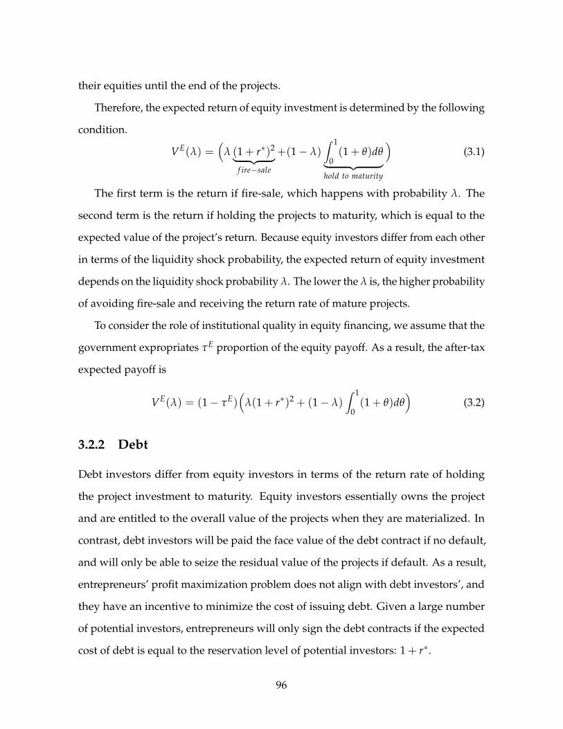
their equities until the end of the projects.

Therefore, the expected return of equity investment is determined by the following

condition.

VE(λ) =(

λ (1 + r∗)2︸︷︷︸f ire−sale

+(1− λ)∫ 1

0(1 + θ)dθ︸︷︷︸

hold to maturity

)(3.1)

The first term is the return if fire-sale, which happens with probability λ. The

second term is the return if holding the projects to maturity, which is equal to the

expected value of the project’s return. Because equity investors differ from each other

in terms of the liquidity shock probability, the expected return of equity investment

depends on the liquidity shock probability λ. The lower the λ is, the higher probability

of avoiding fire-sale and receiving the return rate of mature projects.

To consider the role of institutional quality in equity financing, we assume that the

government expropriates τE proportion of the equity payoff. As a result, the after-tax

expected payoff is

VE(λ) = (1− τE)(

λ(1 + r∗)2 + (1− λ)∫ 1

0(1 + θ)dθ

)(3.2)

3.2.2 Debt

Debt investors differ from equity investors in terms of the return rate of holding

the project investment to maturity. Equity investors essentially owns the project

and are entitled to the overall value of the projects when they are materialized. In

contrast, debt investors will be paid the face value of the debt contract if no default,

and will only be able to seize the residual value of the projects if default. As a result,

entrepreneurs’ profit maximization problem does not align with debt investors’, and

they have an incentive to minimize the cost of issuing debt. Given a large number

of potential investors, entrepreneurs will only sign the debt contracts if the expected

cost of debt is equal to the reservation level of potential investors: 1 + r∗.

96

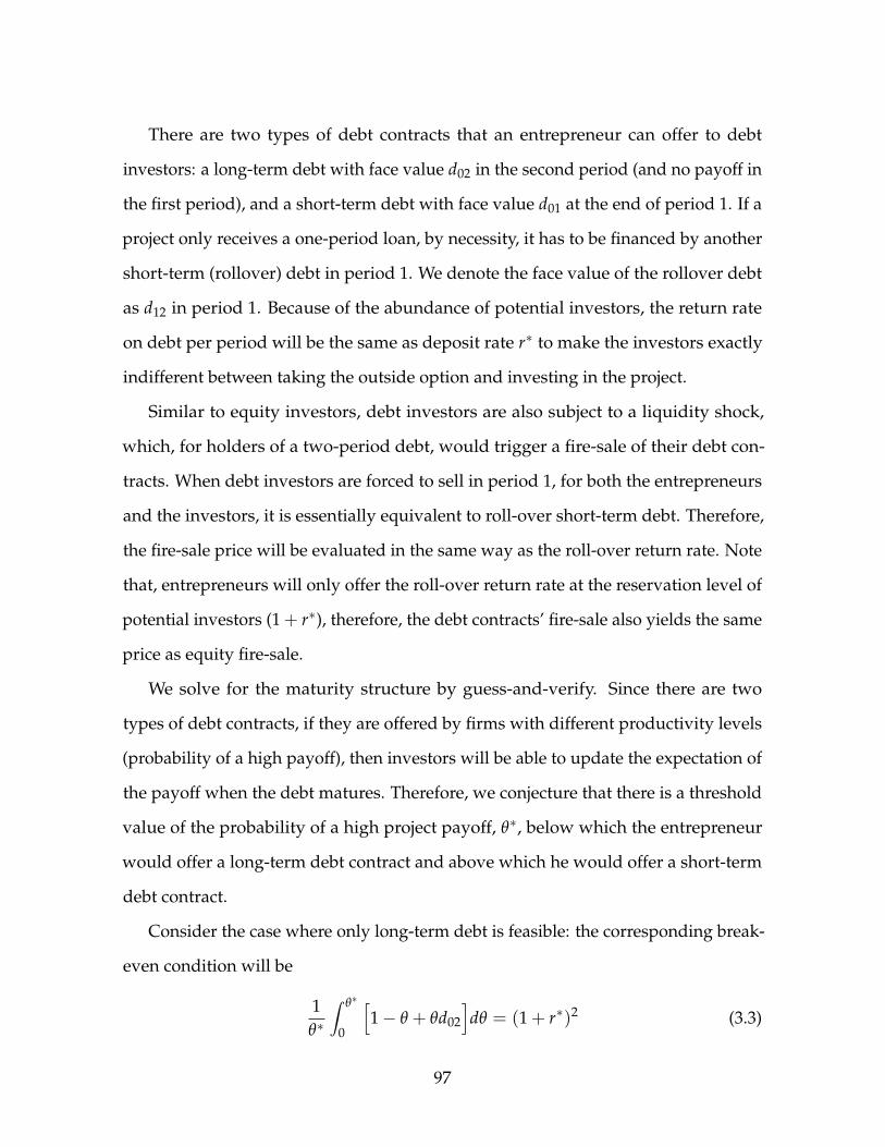
There are two types of debt contracts that an entrepreneur can offer to debt

investors: a long-term debt with face value d02 in the second period (and no payoff in

the first period), and a short-term debt with face value d01 at the end of period 1. If a

project only receives a one-period loan, by necessity, it has to be financed by another

short-term (rollover) debt in period 1. We denote the face value of the rollover debt

as d12 in period 1. Because of the abundance of potential investors, the return rate

on debt per period will be the same as deposit rate r∗ to make the investors exactly

indifferent between taking the outside option and investing in the project.

Similar to equity investors, debt investors are also subject to a liquidity shock,

which, for holders of a two-period debt, would trigger a fire-sale of their debt con-

tracts. When debt investors are forced to sell in period 1, for both the entrepreneurs

and the investors, it is essentially equivalent to roll-over short-term debt. Therefore,

the fire-sale price will be evaluated in the same way as the roll-over return rate. Note

that, entrepreneurs will only offer the roll-over return rate at the reservation level of

potential investors (1 + r∗), therefore, the debt contracts’ fire-sale also yields the same

price as equity fire-sale.

We solve for the maturity structure by guess-and-verify. Since there are two

types of debt contracts, if they are offered by firms with different productivity levels

(probability of a high payoff), then investors will be able to update the expectation of

the payoff when the debt matures. Therefore, we conjecture that there is a threshold

value of the probability of a high project payoff, θ∗, below which the entrepreneur

would offer a long-term debt contract and above which he would offer a short-term

debt contract.

Consider the case where only long-term debt is feasible: the corresponding break-

even condition will be

1θ∗

∫ θ∗

0

[1− θ + θd02

]dθ = (1 + r∗)2 (3.3)

97

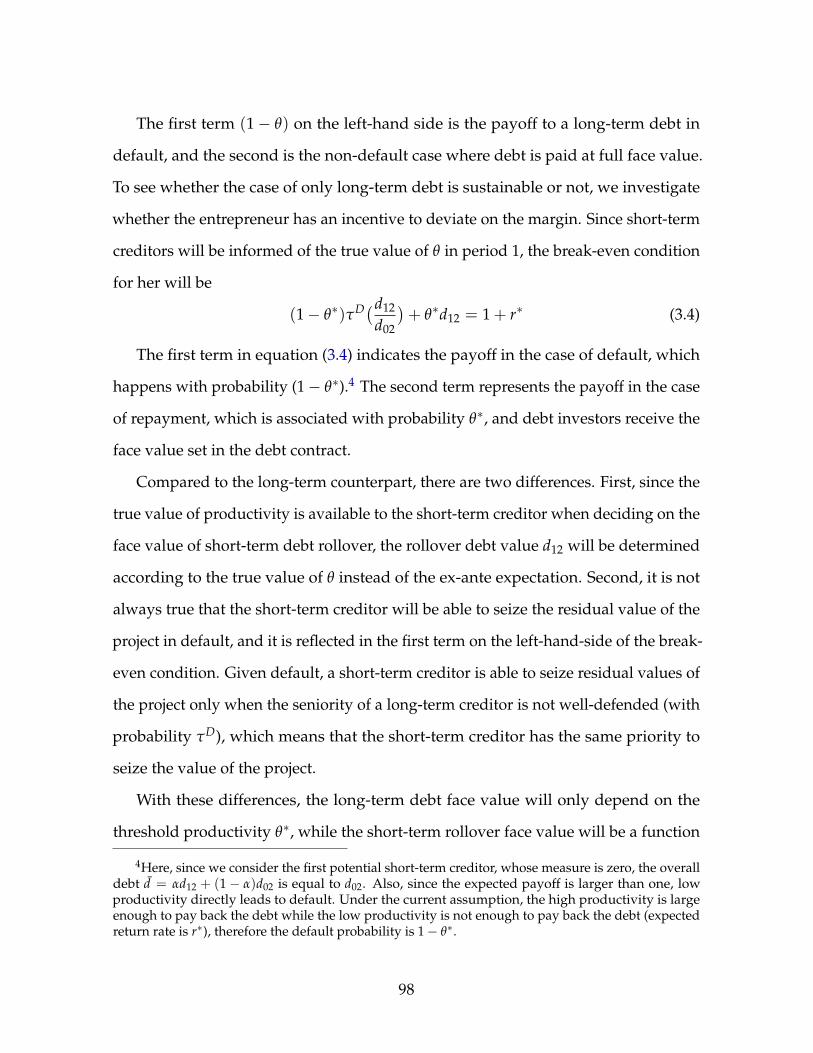
The first term (1− θ) on the left-hand side is the payoff to a long-term debt in

default, and the second is the non-default case where debt is paid at full face value.

To see whether the case of only long-term debt is sustainable or not, we investigate

whether the entrepreneur has an incentive to deviate on the margin. Since short-term

creditors will be informed of the true value of θ in period 1, the break-even condition

for her will be

(1− θ∗)τD(d12

d02

)+ θ∗d12 = 1 + r∗ (3.4)

The first term in equation (3.4) indicates the payoff in the case of default, which

happens with probability (1− θ∗).4 The second term represents the payoff in the case

of repayment, which is associated with probability θ∗, and debt investors receive the

face value set in the debt contract.

Compared to the long-term counterpart, there are two differences. First, since the

true value of productivity is available to the short-term creditor when deciding on the

face value of short-term debt rollover, the rollover debt value d12 will be determined

according to the true value of θ instead of the ex-ante expectation. Second, it is not

always true that the short-term creditor will be able to seize the residual value of the

project in default, and it is reflected in the first term on the left-hand-side of the break-

even condition. Given default, a short-term creditor is able to seize residual values of

the project only when the seniority of a long-term creditor is not well-defended (with

probability τD), which means that the short-term creditor has the same priority to

seize the value of the project.

With these differences, the long-term debt face value will only depend on the

threshold productivity θ∗, while the short-term rollover face value will be a function

4Here, since we consider the first potential short-term creditor, whose measure is zero, the overalldebt d = αd12 + (1− α)d02 is equal to d02. Also, since the expected payoff is larger than one, lowproductivity directly leads to default. Under the current assumption, the high productivity is largeenough to pay back the debt while the low productivity is not enough to pay back the debt (expectedreturn rate is r∗), therefore the default probability is 1− θ∗.

98

of the true productivity θ. After comparing the face values of the long-term (d02) and

short-term (d12) debts, the entrepreneur will choose the lower face value to finance

the project.

To determine the threshold productivity θ∗, we note that at that threshold, the

entrepreneur should be indifferent between offering a short-term and a long-term

debt, which translates to the following condition:

d02(θ∗) = d12(θ

∗) (3.5)

Plugging the indifference condition to the two break-even conditions yields the value

of θ∗.

Proposition 3. The entrepreneur will propose a debt contract based on the project’s produc-

tivity. If θ < θ∗, the borrowing will be in long-term debt. If θ > θ∗, the borrowing will be in

short-term debt. If θ = θ∗, the entrepreneur will be indifferent between the two forms of debt

contracts. θ∗ is determined by (3.3), (3.4), and (3.5).

It can be verified that the entrepreneurs whose project’s productivity is lower

than θ∗ have no incentive to deviate from long-term debt contract, and so with

the entrepreneurs whose project’s productivity is higher than θ∗.5 The intuition

is that since the short-term creditors will be able to work out the true value of θ

when choosing the rollover face value, they will demand a high face value if the

productivity is low.

Those projects with a relatively low productivity will find the long-term face

value (without the knowledge of true productivity on the creditors’ side) to be lower

than the short-term rollover face value. In contrast, projects with a sufficiently high

probability of a high payoff can benefit from a chance to update the creditor about

5Proof is provided in Appendix A.

99

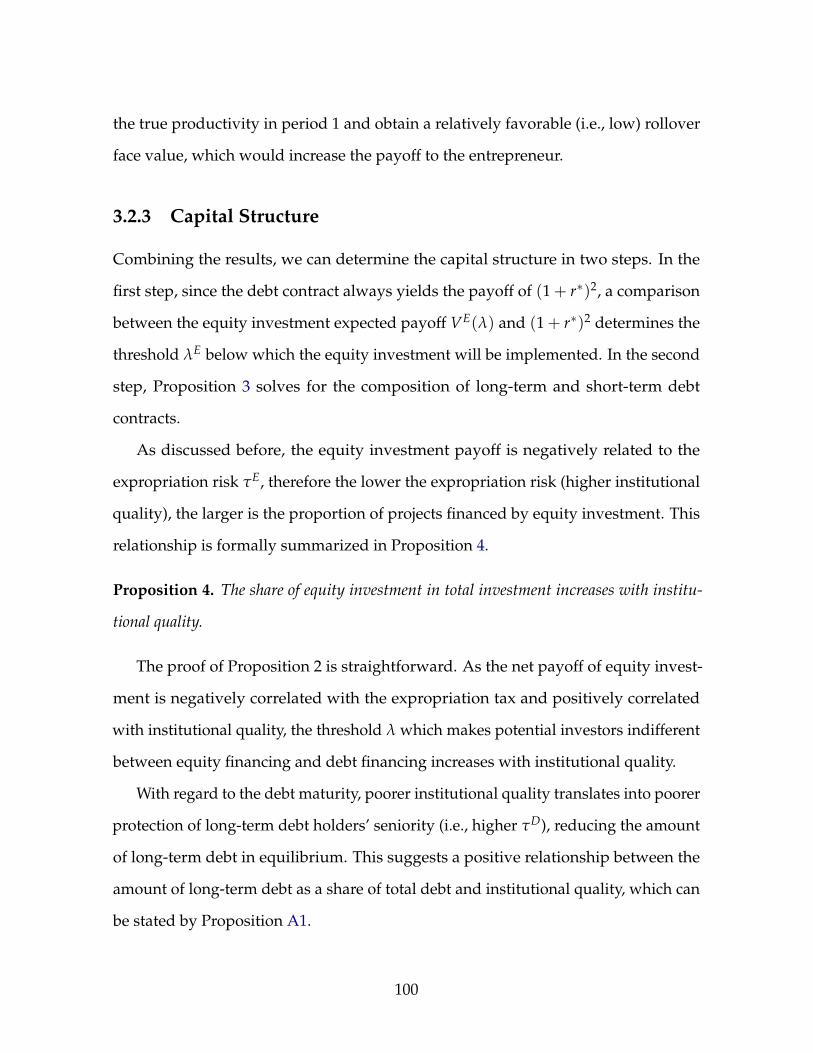
the true productivity in period 1 and obtain a relatively favorable (i.e., low) rollover

face value, which would increase the payoff to the entrepreneur.

3.2.3 Capital Structure

Combining the results, we can determine the capital structure in two steps. In the

first step, since the debt contract always yields the payoff of (1 + r∗)2, a comparison

between the equity investment expected payoff VE(λ) and (1 + r∗)2 determines the

threshold λE below which the equity investment will be implemented. In the second

step, Proposition 3 solves for the composition of long-term and short-term debt

contracts.

As discussed before, the equity investment payoff is negatively related to the

expropriation risk τE, therefore the lower the expropriation risk (higher institutional

quality), the larger is the proportion of projects financed by equity investment. This

relationship is formally summarized in Proposition 4.

Proposition 4. The share of equity investment in total investment increases with institu-

tional quality.

The proof of Proposition 2 is straightforward. As the net payoff of equity invest-

ment is negatively correlated with the expropriation tax and positively correlated

with institutional quality, the threshold λ which makes potential investors indifferent

between equity financing and debt financing increases with institutional quality.

With regard to the debt maturity, poorer institutional quality translates into poorer

protection of long-term debt holders’ seniority (i.e., higher τD), reducing the amount

of long-term debt in equilibrium. This suggests a positive relationship between the

amount of long-term debt as a share of total debt and institutional quality, which can

be stated by Proposition A1.

100

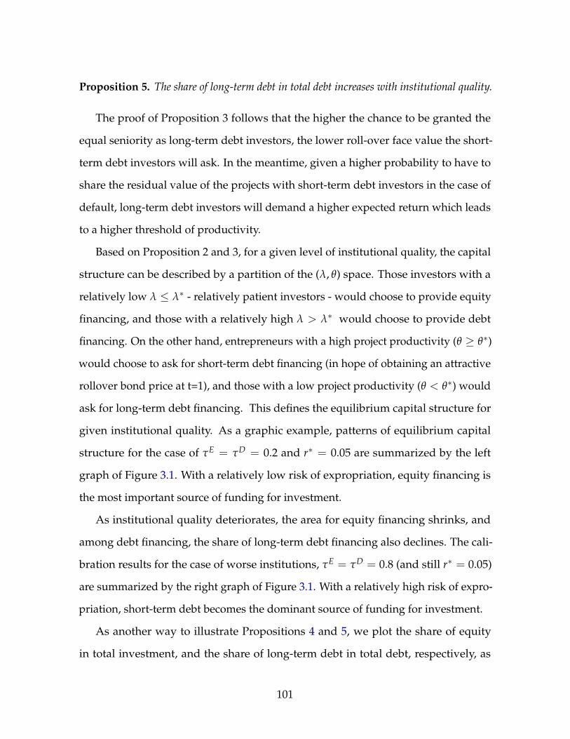
Proposition 5. The share of long-term debt in total debt increases with institutional quality.

The proof of Proposition 3 follows that the higher the chance to be granted the

equal seniority as long-term debt investors, the lower roll-over face value the short-

term debt investors will ask. In the meantime, given a higher probability to have to

share the residual value of the projects with short-term debt investors in the case of

default, long-term debt investors will demand a higher expected return which leads

to a higher threshold of productivity.

Based on Proposition 2 and 3, for a given level of institutional quality, the capital

structure can be described by a partition of the (λ, θ) space. Those investors with a

relatively low λ ≤ λ∗ - relatively patient investors - would choose to provide equity

financing, and those with a relatively high λ > λ∗ would choose to provide debt

financing. On the other hand, entrepreneurs with a high project productivity (θ ≥ θ∗)

would choose to ask for short-term debt financing (in hope of obtaining an attractive

rollover bond price at t=1), and those with a low project productivity (θ < θ∗) would

ask for long-term debt financing. This defines the equilibrium capital structure for

given institutional quality. As a graphic example, patterns of equilibrium capital

structure for the case of τE = τD = 0.2 and r∗ = 0.05 are summarized by the left

graph of Figure 3.1. With a relatively low risk of expropriation, equity financing is

the most important source of funding for investment.

As institutional quality deteriorates, the area for equity financing shrinks, and

among debt financing, the share of long-term debt financing also declines. The cali-

bration results for the case of worse institutions, τE = τD = 0.8 (and still r∗ = 0.05)

are summarized by the right graph of Figure 3.1. With a relatively high risk of expro-

priation, short-term debt becomes the dominant source of funding for investment.

As another way to illustrate Propositions 4 and 5, we plot the share of equity

in total investment, and the share of long-term debt in total debt, respectively, as

101

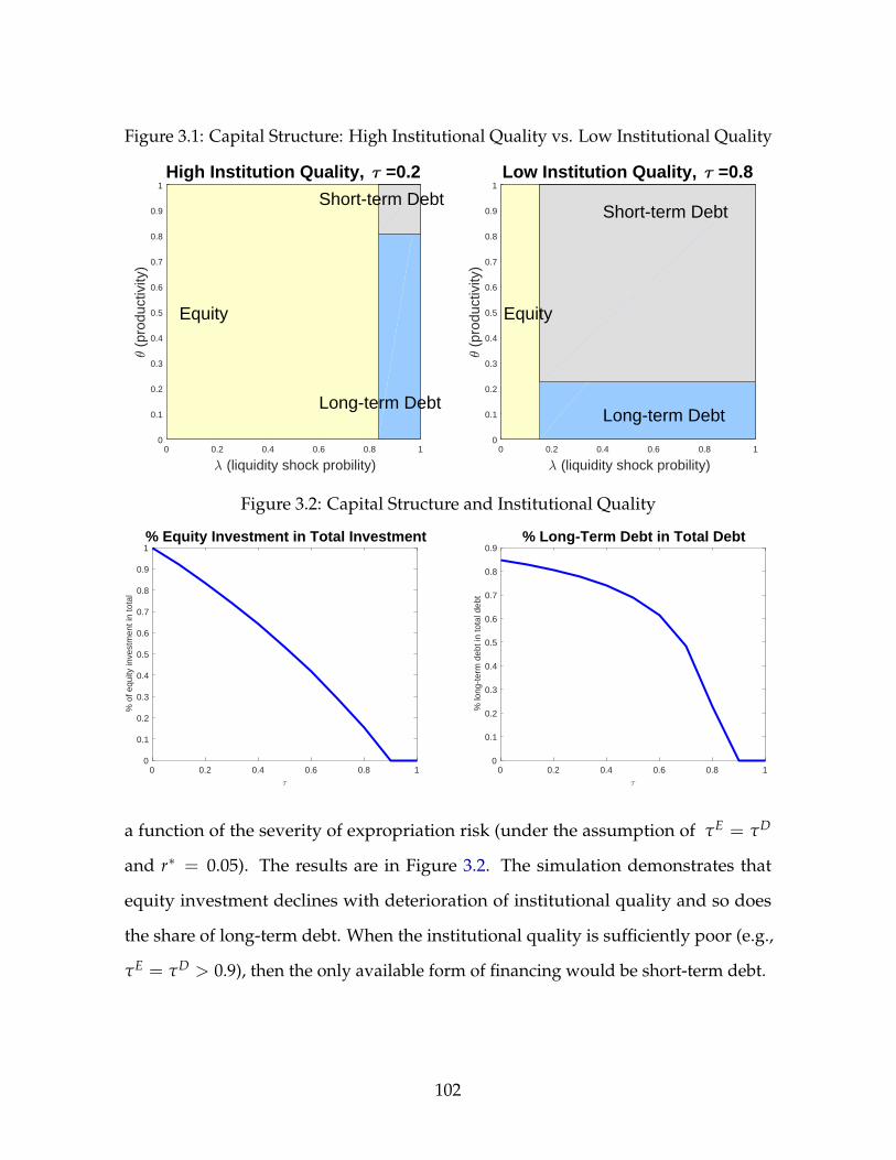
Figure 3.1: Capital Structure: High Institutional Quality vs. Low Institutional Quality

0 0.2 0.4 0.6 0.8 1

(liquidity shock probility)

0

0.1

0.2

0.3

0.4

0.5

0.6

0.7

0.8

0.9

1

(pr

oduc

tivity

)

High Institution Quality, =0.2

Equity

Long-term Debt

Short-term Debt

0 0.2 0.4 0.6 0.8 1

(liquidity shock probility)

0

0.1

0.2

0.3

0.4

0.5

0.6

0.7

0.8

0.9

1

(pr

oduc

tivity

)

Low Institution Quality, =0.8

Equity

Long-term Debt

Short-term Debt

Figure 3.2: Capital Structure and Institutional Quality

0 0.2 0.4 0.6 0.8 10

0.1

0.2

0.3

0.4

0.5

0.6

0.7

0.8

0.9

1

% o

f equ

ity in

vest

men

t in

tota

l

% Equity Investment in Total Investment

0 0.2 0.4 0.6 0.8 10

0.1

0.2

0.3

0.4

0.5

0.6

0.7

0.8

0.9

% lo

ng-t

erm

deb

t in

tota

l deb

t

% Long-Term Debt in Total Debt

a function of the severity of expropriation risk (under the assumption of τE = τD

and r∗ = 0.05). The results are in Figure 3.2. The simulation demonstrates that

equity investment declines with deterioration of institutional quality and so does

the share of long-term debt. When the institutional quality is sufficiently poor (e.g.,

τE = τD > 0.9), then the only available form of financing would be short-term debt.

102

3.3 The Data

In this section, we introduce the datasets that we employ for the empirical analysis

on the relationship between capital structure and institutional quality. Our empirical

exercise will start with the composition of a nation’s external liabilities from balance-

of-payments data: the share of equity (including FDI6) in total external financing, and

the share of long-term debt in total external debt.

We combine two primary data sources: the External Wealth of Nations (EWN)

Dataset data from Lane and Milesi-Ferretti (2007), and the Quarterly External Debt

(QED) Statistics maintained jointly by BIS, IMF, and the World Bank. The EWN

Dataset provides a detailed break-down of international investment positions by

investment type at an annual frequency for most IMF member countries. We define

the share of equity in the total financing of each country i at year t by:

equityit =FDI liabilitiesit + portfolio equity liabilitiesit

total liabilitiesit

Since the EWN Dataset does not contain information on the maturity structure of

loans and deposits, we make use of the relatively new QED Statistics, which collects

the external debt of each country by maturity at a quarterly frequency starting from

1998. We calculate the share of long-term debt in total debt as follows:

long-termit =long-term debt of commercial banksit + long-term debt of other sectorsit

total debt of commercial banks and other sectorsit

The final data set includes an unbalanced panel of the equity shares for 123 countries

with a maximum time span from 1998 to 2011, and an unbalanced panel of the

long-term debt shares for 93 countries with a maximum span from 1998 to 2014.

6FDI is included in equity financing here. There has been work discussing that part of FDI is in theform of intra-firm debt financing within multinational firms. However, what matters most is whatform it is reported because it will determine in what way it will be affected by institutional quality.For instance, even if an FDI is in fact debt financing, as it is reported officially as FDI it will be subjectto the regulations with respect to FDI. That said, in Appendix D we still separately analyze FDI andequity portfolio investment for robustness check.

103

Other macro statistics such as real GDP per capita, private sector debt as a share

of GDP (a proxy for level of the financial development), and trade volume as a share

of GDP (a proxy for the trade openness), are relatively standard and come from the

World Development Indicators (WDI) database of the World Bank.

The institutional quality data is compiled from the World Bank Institute (WBI).

Each year, the WBI uses all available data on institutional quality and proposes a set of

six measures: control of corruption, government efficiency, political stability, regula-

tory quality, rule of law, and voice and accountability. All the indices are constructed

in such a way that each is bound between (-2, +2), and a higher value means a higher

quality of institution. Note, while the six dimensions can in principle capture different

aspects of a country’s public institutions and governance, the pairwise correlations

among them are all positive and in excess of 70%. The exact pairwise correlations are

reported in Table C1. Therefore, out of practical considerations, we will use the simple

average of the six measures as a composite measure of the quality of institutions. The

summary statistics of the variables on the nation’s external financing are reported in

Table C2.

On the domestic side, aggregate measures of capital structure are relatively scarce7,

so we turn to firm-level micro data. There are two data samples that we constructed:

a world-wide sample of listed firms from Worldscope and an European firms sample

(both listed and private) from Amadeus of Bureau van Dijk.8 Both of them have their

own merits as the former one provides a comprehensive picture of the listed firms

from different types of countries and the latter one offers a close look at both the

listed and the private firms. For each firm in the sample, we define the share of equity

7The World Financial Development dataset from the World Bank contains the information on themeasures of financing, but the data is only available for major emerging countries. Also, the measuresare based on firm survey whose sample is relatively small compared to the existing firm-level datasets.

8The results of Amadeus sample is in Appendix C.

104

financing and the share of long-term debt as follows:

equity f t =shareholders funds f t

total liability f t

long-term f t =long-term debt f t

total debt f t

After excluding the financial sector and public administration sector along with

outliers, the Worldscope sample contains 130,167 firms from 2003 to 2015, and the

Amadeus sample yields over 3 million observations from 2004 to 2015. The country

composition and summary statistics can be found in Table C3, Table C4, Table C6,

and Table C7, respectively.

3.4 Capital Structure of External Financing

Based on the theoretical results, there are two hypotheses that we would like to test

the relationship between capital structure and institutional quality.

Hypothesis 1: The share of equity financing is positively correlated with institutional

quality.

Hypothesis 2: The share of long-term debt financing is positively correlated with

institutional quality.As we discussed before, the underlying mechanism of the first hypothesis is that

the improvement in institutional quality reduces expropriation risk and motivates

investors to pursue ownership of target firm’s equity, and the second hypothesis is

the channel that better institutional quality enhances the seniority of long-term debt

and eases the investor’s concern of debt dilution.

To begin with, we plot the relationship between capital structure and institutional

105

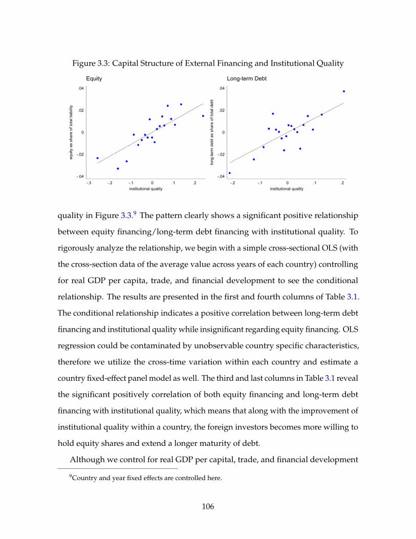
Figure 3.3: Capital Structure of External Financing and Institutional Quality

-.04

-.02

0

.02

.04

equi

ty a

s sh

are

of to

tal l

iabi

lity

-.3 -.2 -.1 0 .1 .2institutional quality

Equity

-.04

-.02

0

.02

.04

long

-term

deb

t as

shar

e of

tota

l deb

t

-.2 -.1 0 .1 .2institutional quality

Long-term Debt

quality in Figure 3.3.9 The pattern clearly shows a significant positive relationship

between equity financing/long-term debt financing with institutional quality. To

rigorously analyze the relationship, we begin with a simple cross-sectional OLS (with

the cross-section data of the average value across years of each country) controlling

for real GDP per capita, trade, and financial development to see the conditional

relationship. The results are presented in the first and fourth columns of Table 3.1.

The conditional relationship indicates a positive correlation between long-term debt

financing and institutional quality while insignificant regarding equity financing. OLS

regression could be contaminated by unobservable country specific characteristics,

therefore we utilize the cross-time variation within each country and estimate a

country fixed-effect panel model as well. The third and last columns in Table 3.1 reveal

the significant positively correlation of both equity financing and long-term debt

financing with institutional quality, which means that along with the improvement of

institutional quality within a country, the foreign investors becomes more willing to

hold equity shares and extend a longer maturity of debt.

Although we control for real GDP per capital, trade, and financial development

9Country and year fixed effects are controlled here.

106

(consistent with literature, such as Faria and Mauro (2009)), there can still exist

unobservables that potentially contaminate the estimates. To address the endogeneity

issue, we employ an instrumental variable (IV) approach. Alesina and Zhuravskaya

(2011) suggest that linguistically more segregated countries, i.e., those where different

linguistic groups live more spatially separated, have a lower quality of government.

We use language segregation as an IV for institutional quality. As constructed by

Alesina and Zhuravskaya (2011), the index of segregation is a population-weighted

average of homogeneity across groups within country based on historical data. As

the index of segregation does not allow across-time variation, we run 2SLS on the

cross-section sample.

The second and the fifth columns in Table 3.1 present the 2SLS results. Firstly,

consistent with Alesina and Zhuravskaya (2011), the significant correlation between

institutional quality and language segregation supports the strongly negative rela-

tionship between linguistic segregation and institutional quality. Secondly, the weak

IV test validates language segregation as a strong instrument for institutional quality.

Thirdly, the IV estimates indicate strongly positive impact of institutional quality on

boosting cross-border equity financing and long-term external debt. An improvement

in institutional quality by one standard deviation (about 0.85) would increase the

share of equity in total liability by 35% (more than two standard deviations) and raise

the share of long-term debt in total debt by 15% (about 0.7 standard deviation). These

effects are both economically significant and statistically significant.

Besides the baseline analysis, we conduct three sets of robustness checks. First, one

concern about the cross-sectional analysis is that different countries enter the sample

in different years due to data availability, therefore the effect of institutional quality

on external capital structure may be driven by the difference in the development

stage across countries. To address this issue, we take a balanced panel from 2002 to

107

2014 and redo the IV regressions. As shown in Table 3.2, the effects of institutional

quality in promoting equity and long-term debt financing remain significant.

Second, foreign reserves could be an omitted variable. As part of development,

central banks may accumulate foreign reserves as macro-prudential policy, in the

meantime, government may strengthen institutional quality. Therefore, foreign

reserves may be correlated with institutional quality. Moreover, higher foreign

reserves reduces the financial risk of the country, therefore international investors are

willing to conduct equity investment and long-term debt investment. To check this

omitted variable bias, we add foreign reserves as an additional control in the baseline

specification. Table 3.3 presents the results: foreign reserve is indeed positively

correlated with equity financing share and long-term debt share, but the positive

effect generated by institutional quality improvement stands significant.

Thirdly, given the dependent variable is the proportion of equity or debt financing,

which takes value between zero and one, it worth checking with the Logit regression

to see whether the linear regression results are robust. Table 3.4 shows the regressions

with the Logit specifications, and the positive correlation between equity or long-term

debt and institutional quality remains very robust.

3.5 Structure of Domestic Financing and Institutional

Quality

While the previous section examines the structure of the external liabilities of nations,

we now turn attention to capital structure at the firm level. While firms can obtain

financing from both domestic and international sources, domestic financing would be

the more important source in most cases. For a given country (and therefore a given

national level governance), there will be a distribution of capital structure across firms.

108

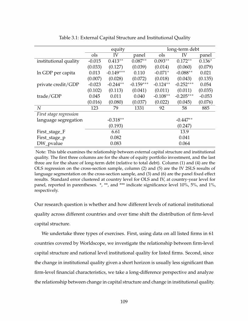
Table 3.1: External Capital Structure and Institutional Quality

equity long-term debtols IV panel ols IV panel

institutional quality -0.015 0.413∗∗ 0.087∗∗ 0.093∗∗ 0.172∗∗ 0.136∗

(0.033) (0.127) (0.039) (0.014) (0.060) (0.079)ln GDP per capita 0.013 -0.149∗∗∗ 0.110 -0.071∗ -0.088∗∗ 0.021

(0.007) (0.028) (0.072) (0.018) (0.043) (0.135)private credit/GDP -0.023 -0.244∗∗ -0.159∗∗∗ -0.124∗∗ -0.252∗∗∗ 0.054

(0.102) (0.113) (0.041) (0.011) (0.011) (0.035)trade/GDP 0.045 0.011 0.040 -0.108∗∗ -0.205∗∗∗ -0.053

(0.016) (0.080) (0.037) (0.022) (0.045) (0.076)N 123 79 1331 92 58 885First stage regressionlanguage segregation -0.318∗∗ -0.447∗∗

(0.193) (0.247)First_stage_F 6.61 13.9First_stage_p 0.082 0.041DW_pvalue 0.083 0.064

Note: This table examines the relationship between external capital structure and institutionalquality. The first three columns are for the share of equity portfolio investment, and the lastthree are for the share of long-term debt (relative to total debt). Column (1) and (4) are theOLS regression on the cross-section sample, column (2) and (5) are the IV 2SLS results oflanguage segmentation on the cross-section sample, and (3) and (6) are the panel fixed effectresults. Standard error clustered at country level for OLS and IV, at country-year level forpanel, reported in parentheses. *, **, and *** indicate significance level 10%, 5%, and 1%,respectively.

Our research question is whether and how different levels of national institutional

quality across different countries and over time shift the distribution of firm-level

capital structure.

We undertake three types of exercises. First, using data on all listed firms in 61

countries covered by Worldscope, we investigate the relationship between firm-level

capital structure and national level institutional quality for listed firms. Second, since

the change in institutional quality given a short horizon is usually less significant than

firm-level financial characteristics, we take a long-difference perspective and analyze

the relationship between change in capital structure and change in institutional quality.

109

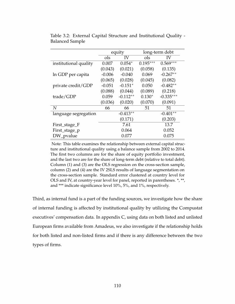
Table 3.2: External Capital Structure and Institutional Quality -Balanced Sample

equity long-term debtols IV ols IV

institutional quality 0.007 0.054∗ 0.195∗∗∗ 0.569∗∗∗

(0.043) (0.021) (0.058) (0.135)ln GDP per capita -0.006 -0.040 0.069 -0.267∗∗

(0.065) (0.028) (0.045) (0.082)private credit/GDP -0.051 -0.151∗ 0.050 -0.482∗∗

(0.088) (0.044) (0.089) (0.218)trade/GDP 0.059 -0.112∗∗ 0.130∗ -0.335∗∗∗

(0.036) (0.020) (0.070) (0.091)N 66 66 51 51language segregation -0.413∗∗ -0.401∗∗


Note: This table examines the relationship between external capital struc-ture and institutional quality using a balance sample from 2002 to 2014.The first two columns are for the share of equity portfolio investment,and the last two are for the share of long-term debt (relative to total debt).Column (1) and (3) are the OLS regression on the cross-section sample,column (2) and (4) are the IV 2SLS results of language segmentation onthe cross-section sample. Standard error clustered at country level forOLS and IV, at country-year level for panel, reported in parentheses. *, **,and *** indicate significance level 10%, 5%, and 1%, respectively.

Third, as internal fund is a part of the funding sources, we investigate how the share

of internal funding is affected by institutional quality by utilizing the Compustat

executives’ compensation data. In appendix C, using data on both listed and unlisted

European firms available from Amadeus, we also investigate if the relationship holds

for both listed and non-listed firms and if there is any difference between the two

types of firms.

110

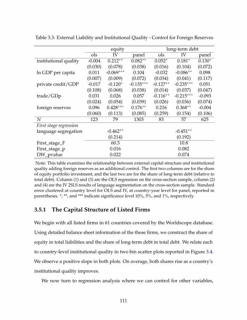
Table 3.3: External Liability and Institutional Quality - Control for Foreign Reserves

equity long-term debtols IV panel ols IV panel

institutional quality -0.004 0.212∗∗ 0.082∗∗ 0.052∗ 0.181∗ 0.130∗

(0.030) (0.078) (0.038) (0.016) (0.104) (0.072)ln GDP per capita 0.011 -0.069∗∗∗ 0.104 -0.032 -0.086∗∗ 0.098

(0.007) (0.009) (0.072) (0.034) (0.041) (0.117)private credit/GDP -0.017 -0.120∗ -0.135∗∗∗ -0.127∗∗ -0.235∗∗∗ 0.051

(0.108) (0.068) (0.038) (0.014) (0.037) (0.047)trade/GDp 0.031 0.026 0.057 -0.116∗∗ -0.215∗∗∗ -0.093

(0.024) (0.054) (0.039) (0.026) (0.036) (0.074)foreign reserves 0.096 0.428∗∗∗ 0.176∗∗ 0.216 0.368∗∗ -0.004



Note: This table examines the relationship between external capital structure and institutionalquality adding foreign reserves as an additional control. The first two columns are for the shareof equity portfolio investment, and the last two are for the share of long-term debt (relative tototal debt). Column (1) and (3) are the OLS regression on the cross-section sample, column (2)and (4) are the IV 2SLS results of language segmentation on the cross-section sample. Standarderror clustered at country level for OLS and IV, at country-year level for panel, reported inparentheses. *, **, and *** indicate significance level 10%, 5%, and 1%, respectively.

3.5.1 The Capital Structure of Listed Firms

We begin with all listed firms in 61 countries covered by the Worldscope database.

Using detailed balance sheet information of the these firms, we construct the share of

equity in total liabilities and the share of long-term debt in total debt. We relate each

to country-level institutional quality in two bin scatter plots reported in Figure 3.4.

We observe a positive slope in both plots. On average, both shares rise as a country’s

institutional quality improves.

We now turn to regression analysis where we can control for other variables,

111

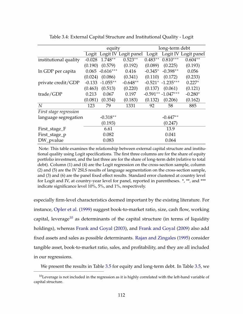
Table 3.4: External Capital Structure and Institutional Quality - Logit

equity long-term debtLogit Logit IV Logit panel Logit Logit IV Logit panel

institutional quality -0.028 1.748∗∗ 0.523∗∗ 0.483∗∗ 0.810∗∗∗ 0.604∗∗

(0.190) (0.579) (0.192) (0.089) (0.225) (0.193)ln GDP per capita 0.065 -0.616∗∗∗ 0.416 -0.345∗ -0.398∗∗ 0.056

(0.024) (0.086) (0.341) (0.110) (0.172) (0.233)private credit/GDP -0.133 -1.055∗∗ -0.648∗∗ -0.521∗ -1.235∗∗∗ 0.227∗

(0.463) (0.513) (0.220) (0.137) (0.061) (0.121)trade/GDP 0.213 0.067 0.197 -0.591∗∗ -1.047∗∗∗ -0.280∗



Note: This table examines the relationship between external capital structure and institu-tional quality using Logit specifications. The first three columns are for the share of equityportfolio investment, and the last three are for the share of long-term debt (relative to totaldebt). Column (1) and (4) are the Logit regression on the cross-section sample, column(2) and (5) are the IV 2SLS results of language segmentation on the cross-section sample,and (3) and (6) are the panel fixed effect results. Standard error clustered at country levelfor Logit and IV, at country-year level for panel, reported in parentheses. *, **, and ***indicate significance level 10%, 5%, and 1%, respectively.

especially firm-level characteristics deemed important by the existing literature. For

instance, Opler et al. (1999) suggest book-to-market ratio, size, cash flow, working

capital, leverage10 as determinants of the capital structure (in terms of liquidity

holdings), whereas Frank and Goyal (2003), and Frank and Goyal (2009) also add

fixed assets and sales as possible determinants. Rajan and Zingales (1995) consider

tangible asset, book-to-market ratio, sales, and profitability, and they are all included

in our regressions.

We present the results in Table 3.5 for equity and long-term debt. In Table 3.5, we

10Leverage is not included in the regression as it is highly correlated with the left-hand variable ofcapital structure.

112

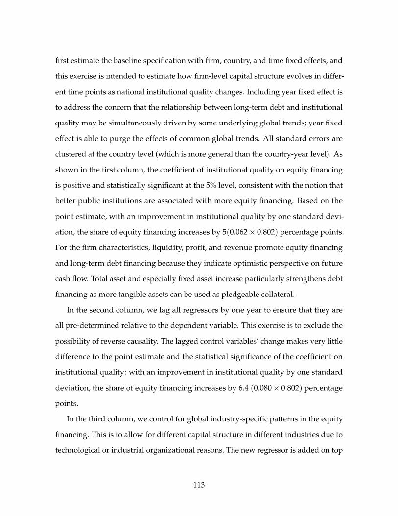
first estimate the baseline specification with firm, country, and time fixed effects, and

this exercise is intended to estimate how firm-level capital structure evolves in differ-

ent time points as national institutional quality changes. Including year fixed effect is

to address the concern that the relationship between long-term debt and institutional

quality may be simultaneously driven by some underlying global trends; year fixed

effect is able to purge the effects of common global trends. All standard errors are

clustered at the country level (which is more general than the country-year level). As

shown in the first column, the coefficient of institutional quality on equity financing

is positive and statistically significant at the 5% level, consistent with the notion that

better public institutions are associated with more equity financing. Based on the

point estimate, with an improvement in institutional quality by one standard devi-

ation, the share of equity financing increases by 5(0.062× 0.802) percentage points.

For the firm characteristics, liquidity, profit, and revenue promote equity financing

and long-term debt financing because they indicate optimistic perspective on future

cash flow. Total asset and especially fixed asset increase particularly strengthens debt

financing as more tangible assets can be used as pledgeable collateral.

In the second column, we lag all regressors by one year to ensure that they are

all pre-determined relative to the dependent variable. This exercise is to exclude the

possibility of reverse causality. The lagged control variables’ change makes very little

difference to the point estimate and the statistical significance of the coefficient on

institutional quality: with an improvement in institutional quality by one standard

deviation, the share of equity financing increases by 6.4 (0.080× 0.802) percentage

points.

In the third column, we control for global industry-specific patterns in the equity

financing. This is to allow for different capital structure in different industries due to

technological or industrial organizational reasons. The new regressor is added on top

113

of controlling for firm fixed effects and global time trends. Unsurprisingly, firm level

equity financing share is positively correlated with average equity financing across

all firms in the same industry in the world. Although, with this additional control,

the coefficient on national institutional quality becomes smaller, it is still positive and

statistically significant and also close to the baseline estimate in the first column.

In the fourth column, similar to the external capital structure analysis, we check

the robustness of the results to Logit specification. The Logit panel fixed effect takes

care of the dependent variable ranging between zero and one. As shown in the table,

the positive relationship remains positive and significant.

In the last four columns of Table 3.5, we present a similar set of analysis for long-

term financing as a share of total debt financing. Same as the case for long-term

debt financing, in the fifth columns, we include firm, country, and year fixed effects.

The coefficient on institutional quality are both positive and statistically significant

at the 10% level. The point estimate indicates that with an improvement in public

institutional quality by one standard deviation, the equity share in total external

financing tends to go up by 0.802× 0.124 = 9.9 percentage points. The alternative

specifications with lagged control variables and industry-specific long-term debt

financing, in the last two columns, respectively, confirm the significant positive

relationship between institutional quality and long-term debt financing. The results

also provide a strong support for the baseline regression as the point estimate for the

relationship between institutional quality and long-term debt financing stays around

0.12 in all three specifications.

We can obtain more precise information on corporate bonds at issuance from the

Mergent Fixed Income Securities database (FISD). FISD reports issuing date, amount,

spread, and maturity. A given firm can of course issue multiple bonds in a year.

Therefore, for a given firm in a given year, we can compute the average maturity of

114

Figure 3.4: Capital Structure and Institutional Quality (Worldscope)

.43

.44

.45

.46

.47

equi

ty a

s sh

are

of to

tal l

iabi

lity

.6 .7 .8 .9 1institutional quality

Equity

.49

.5

.51

.52

.53

long

-term

deb

t as

shar

e of

tota

l deb

t

.6 .7 .8 .9institutional quality

Long-term Debt

its bonds weighted by the proceeds of each bond. We investigate the relationship

between the average bond maturity (at the firm level) and institutional quality (at the

national level). We use firm characteristics from Worldscope (after matching the firms

in the two databases) as controls, and we cluster all standard errors at the country

level.

The results are reported in Table 3.6. We see that the average maturity of corporate

bonds is significant positively correlated with institutional quality, and the estimates

in all three specifications are positive and significant at 5% level. Generally speaking,

with a standard deviation improvement in institutional quality, the average maturity

of corporate bonds would go up by 0.72 (0.24× 3.0) years.

To conclude, with better public governance, both equity share in total financing

and the maturity of debt would go up. The magnitude of the correlation is both

statistically and economically significant. These patterns are consistent with the

theory presented in Section 2 that high institutional quality is associated with external

financing tilting toward equity and long maturity debt.11

Next, we further inspect the aspect of institutional quality that is the most impor-

11The effect of institutional quality on capital structure could potentially differ along different levelsof institutional quality, and Appendix E explores this property.

115

tant in influencing capital structure. So far, our measure of institutional quality is

the average of six indicators from the World Bank’s World Governance Indicators:

corruption control, government efficiency, political stability, regulation quality, rule

of law, and voice accountability. While the pairwise correlations among the six indica-

tors are all in excess of 70% (see Table C1), it might be useful nonetheless to see which

subset of governance indicators may be the most relevant for the capital structure

question.

We re-run the regressions on the share of equity financing, where quality of

governance is measured by each of the six indicators individually, and report the

results in Table 3.7. Note that the specification includes firm and year fixed effects, and

the standard errors are clustered at the country level. We see that corruption control,

government efficiency, rule of law, and voice of accountability are the important ones

in explaining the share of equity financing. Of these, the share of equity financing

appears to be most responsive to variations in the strength of control of corruption

and voice of accountability. In comparison, political stability and regulation quality

are not statistically different from zero. These results are perhaps not too surprising

in light of our theory in which the relevant institutions are those that minimize the

expropriation risk of equity holders (e.g., tax on their equity returns).

We do a similar exercise for the share of long-term debt financing in total debt,

and report the results in Table 3.8. In this case, the most significant relationship is

between maturity of debt (measured in both share of long-term debt financing and

the maturity of corporate bond) and rule of law. This result is intuitive as the most

relevant institutional quality for long-term debt holders is how their long-term debt

holding are well protected without debt dilution, and rule of law plays a crucial role

in protecting the right of long-term debt holders against the dilution risk.

116

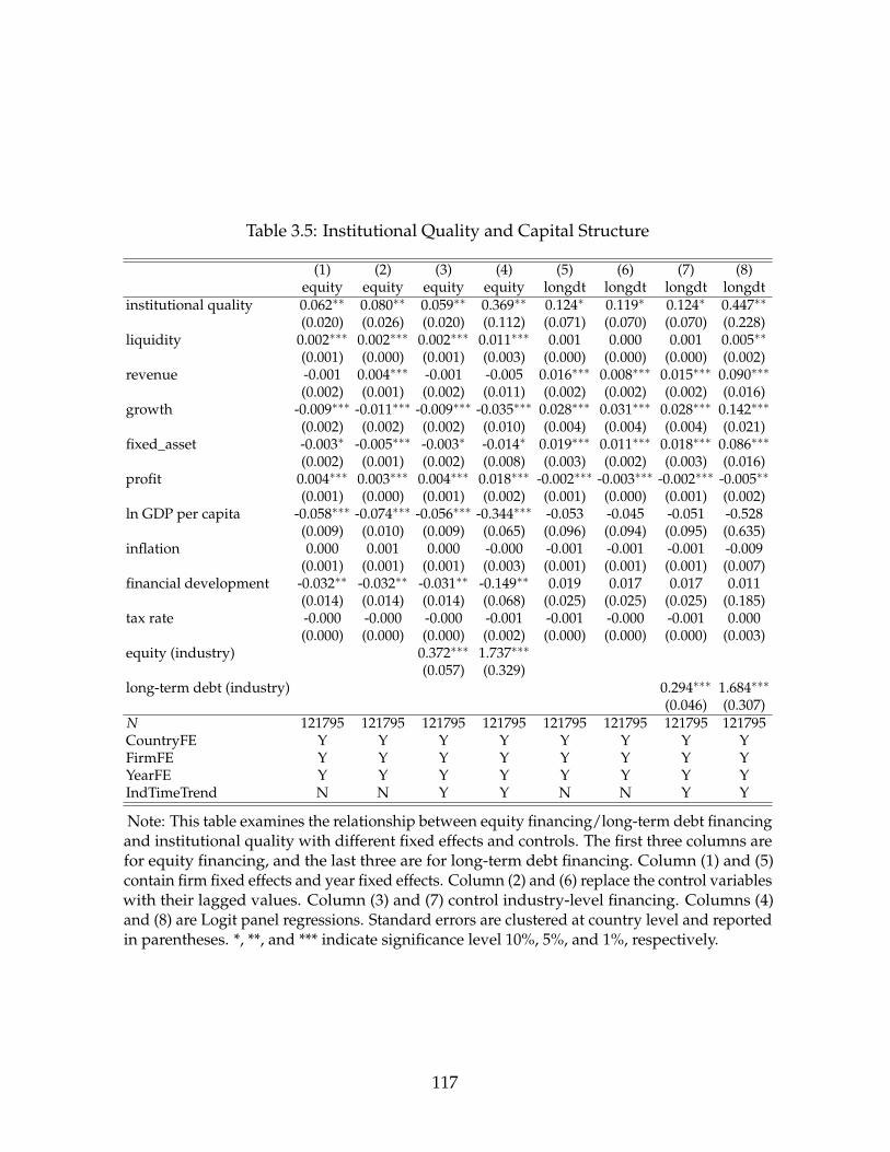
Table 3.5: Institutional Quality and Capital Structure

(1) (2) (3) (4) (5) (6) (7) (8)equity equity equity equity longdt longdt longdt longdt

institutional quality 0.062∗∗ 0.080∗∗ 0.059∗∗ 0.369∗∗ 0.124∗ 0.119∗ 0.124∗ 0.447∗∗

(0.020) (0.026) (0.020) (0.112) (0.071) (0.070) (0.070) (0.228)liquidity 0.002∗∗∗ 0.002∗∗∗ 0.002∗∗∗ 0.011∗∗∗ 0.001 0.000 0.001 0.005∗∗

(0.001) (0.000) (0.001) (0.003) (0.000) (0.000) (0.000) (0.002)revenue -0.001 0.004∗∗∗ -0.001 -0.005 0.016∗∗∗ 0.008∗∗∗ 0.015∗∗∗ 0.090∗∗∗

(0.002) (0.001) (0.002) (0.011) (0.002) (0.002) (0.002) (0.016)growth -0.009∗∗∗ -0.011∗∗∗ -0.009∗∗∗ -0.035∗∗∗ 0.028∗∗∗ 0.031∗∗∗ 0.028∗∗∗ 0.142∗∗∗

(0.002) (0.002) (0.002) (0.010) (0.004) (0.004) (0.004) (0.021)fixed_asset -0.003∗ -0.005∗∗∗ -0.003∗ -0.014∗ 0.019∗∗∗ 0.011∗∗∗ 0.018∗∗∗ 0.086∗∗∗

(0.002) (0.001) (0.002) (0.008) (0.003) (0.002) (0.003) (0.016)profit 0.004∗∗∗ 0.003∗∗∗ 0.004∗∗∗ 0.018∗∗∗ -0.002∗∗∗ -0.003∗∗∗ -0.002∗∗∗ -0.005∗∗

(0.001) (0.000) (0.001) (0.002) (0.001) (0.000) (0.001) (0.002)ln GDP per capita -0.058∗∗∗ -0.074∗∗∗ -0.056∗∗∗ -0.344∗∗∗ -0.053 -0.045 -0.051 -0.528

(0.009) (0.010) (0.009) (0.065) (0.096) (0.094) (0.095) (0.635)inflation 0.000 0.001 0.000 -0.000 -0.001 -0.001 -0.001 -0.009

(0.001) (0.001) (0.001) (0.003) (0.001) (0.001) (0.001) (0.007)financial development -0.032∗∗ -0.032∗∗ -0.031∗∗ -0.149∗∗ 0.019 0.017 0.017 0.011

(0.014) (0.014) (0.014) (0.068) (0.025) (0.025) (0.025) (0.185)tax rate -0.000 -0.000 -0.000 -0.001 -0.001 -0.000 -0.001 0.000

(0.000) (0.000) (0.000) (0.002) (0.000) (0.000) (0.000) (0.003)equity (industry) 0.372∗∗∗ 1.737∗∗∗

(0.057) (0.329)long-term debt (industry) 0.294∗∗∗ 1.684∗∗∗

(0.046) (0.307)N 121795 121795 121795 121795 121795 121795 121795 121795CountryFE Y Y Y Y Y Y Y YFirmFE Y Y Y Y Y Y Y YYearFE Y Y Y Y Y Y Y YIndTimeTrend N N Y Y N N Y Y

Note: This table examines the relationship between equity financing/long-term debt financingand institutional quality with different fixed effects and controls. The first three columns arefor equity financing, and the last three are for long-term debt financing. Column (1) and (5)contain firm fixed effects and year fixed effects. Column (2) and (6) replace the control variableswith their lagged values. Column (3) and (7) control industry-level financing. Columns (4)and (8) are Logit panel regressions. Standard errors are clustered at country level and reportedin parentheses. *, **, and *** indicate significance level 10%, 5%, and 1%, respectively.

117

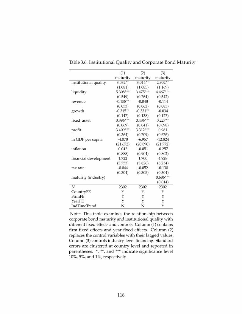
Table 3.6: Institutional Quality and Corporate Bond Maturity

(1) (2) (3)maturity maturity maturity

institutional quality 3.032∗∗ 3.014∗∗ 2.902∗∗

(1.081) (1.085) (1.169)liquidity 5.308∗∗∗ 3.475∗∗∗ 4.467∗∗∗

(0.549) (0.764) (0.542)revenue -0.158∗∗ -0.048 -0.114

(0.053) (0.062) (0.083)growth -0.315∗∗ -0.331∗∗ -0.034

(0.147) (0.138) (0.127)fixed_asset 0.396∗∗∗ 0.436∗∗∗ 0.227∗∗

(0.069) (0.041) (0.098)profit 3.409∗∗∗ 3.312∗∗∗ 0.981

(0.364) (0.709) (0.676)ln GDP per capita -4.078 -6.957 -12.824

(21.672) (20.890) (21.772)inflation 0.042 -0.051 -0.257

(0.888) (0.904) (0.802)financial development 1.722 1.700 4.928

(3.753) (3.826) (3.254)tax rate -0.044 -0.052 -0.130

(0.304) (0.305) (0.304)maturity (industry) 0.686∗∗∗

(0.014)N 2302 2302 2302CountryFE Y Y YFirmFE Y Y YYearFE Y Y YIndTimeTrend N N Y

Note: This table examines the relationship betweencorporate bond maturity and institutional quality withdifferent fixed effects and controls. Column (1) containsfirm fixed effects and year fixed effects. Column (2)replaces the control variables with their lagged values.Column (3) controls industry-level financing. Standarderrors are clustered at country level and reported inparentheses. *, **, and *** indicate significance level10%, 5%, and 1%, respectively.

118

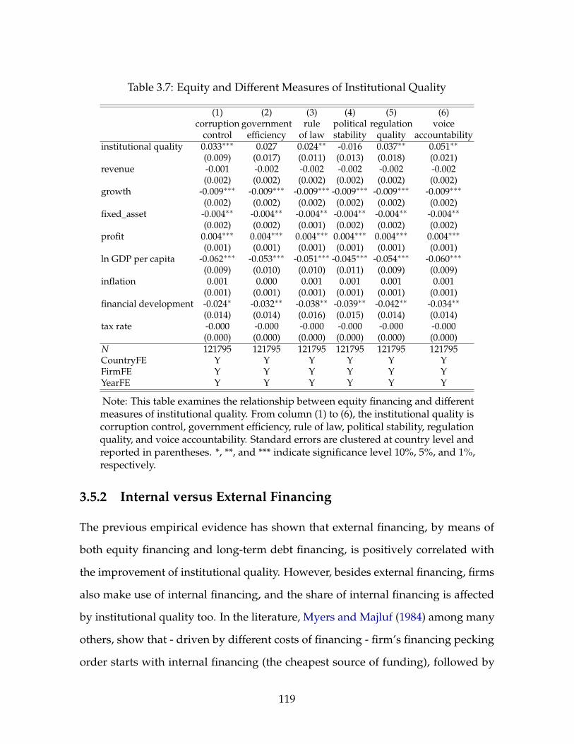
Table 3.7: Equity and Different Measures of Institutional Quality

(1) (2) (3) (4) (5) (6)corruption government rule political regulation voice

control efficiency of law stability quality accountabilityinstitutional quality 0.033∗∗∗ 0.027 0.024∗∗ -0.016 0.037∗∗ 0.051∗∗

(0.009) (0.017) (0.011) (0.013) (0.018) (0.021)revenue -0.001 -0.002 -0.002 -0.002 -0.002 -0.002

(0.002) (0.002) (0.002) (0.002) (0.002) (0.002)growth -0.009∗∗∗ -0.009∗∗∗ -0.009∗∗∗ -0.009∗∗∗ -0.009∗∗∗ -0.009∗∗∗

(0.002) (0.002) (0.002) (0.002) (0.002) (0.002)fixed_asset -0.004∗∗ -0.004∗∗ -0.004∗∗ -0.004∗∗ -0.004∗∗ -0.004∗∗

(0.002) (0.002) (0.001) (0.002) (0.002) (0.002)profit 0.004∗∗∗ 0.004∗∗∗ 0.004∗∗∗ 0.004∗∗∗ 0.004∗∗∗ 0.004∗∗∗

(0.001) (0.001) (0.001) (0.001) (0.001) (0.001)ln GDP per capita -0.062∗∗∗ -0.053∗∗∗ -0.051∗∗∗ -0.045∗∗∗ -0.054∗∗∗ -0.060∗∗∗

(0.009) (0.010) (0.010) (0.011) (0.009) (0.009)inflation 0.001 0.000 0.001 0.001 0.001 0.001

(0.001) (0.001) (0.001) (0.001) (0.001) (0.001)financial development -0.024∗ -0.032∗∗ -0.038∗∗ -0.039∗∗ -0.042∗∗ -0.034∗∗

(0.014) (0.014) (0.016) (0.015) (0.014) (0.014)tax rate -0.000 -0.000 -0.000 -0.000 -0.000 -0.000

(0.000) (0.000) (0.000) (0.000) (0.000) (0.000)N 121795 121795 121795 121795 121795 121795CountryFE Y Y Y Y Y YFirmFE Y Y Y Y Y YYearFE Y Y Y Y Y Y

Note: This table examines the relationship between equity financing and differentmeasures of institutional quality. From column (1) to (6), the institutional quality iscorruption control, government efficiency, rule of law, political stability, regulationquality, and voice accountability. Standard errors are clustered at country level andreported in parentheses. *, **, and *** indicate significance level 10%, 5%, and 1%,respectively.

3.5.2 Internal versus External Financing

The previous empirical evidence has shown that external financing, by means of

both equity financing and long-term debt financing, is positively correlated with

the improvement of institutional quality. However, besides external financing, firms

also make use of internal financing, and the share of internal financing is affected

by institutional quality too. In the literature, Myers and Majluf (1984) among many

others, show that - driven by different costs of financing - firm’s financing pecking

order starts with internal financing (the cheapest source of funding), followed by

119

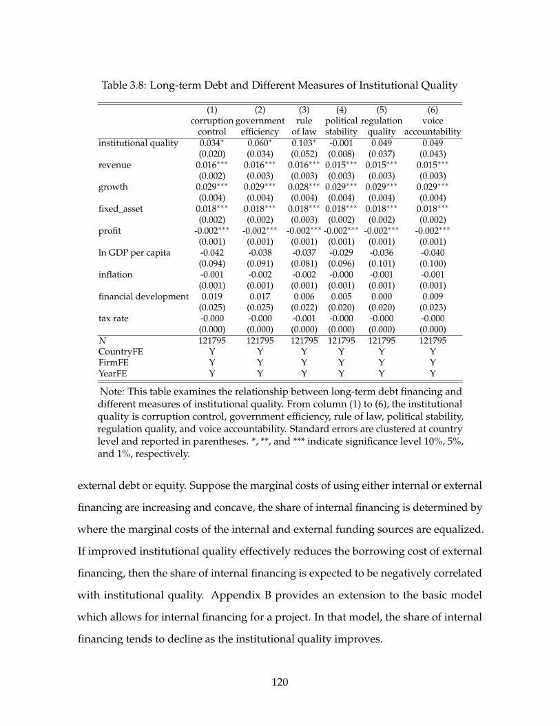
Table 3.8: Long-term Debt and Different Measures of Institutional Quality

(1) (2) (3) (4) (5) (6)corruption government rule political regulation voice

control efficiency of law stability quality accountabilityinstitutional quality 0.034∗ 0.060∗ 0.103∗ -0.001 0.049 0.049

(0.020) (0.034) (0.052) (0.008) (0.037) (0.043)revenue 0.016∗∗∗ 0.016∗∗∗ 0.016∗∗∗ 0.015∗∗∗ 0.015∗∗∗ 0.015∗∗∗

(0.002) (0.003) (0.003) (0.003) (0.003) (0.003)growth 0.029∗∗∗ 0.029∗∗∗ 0.028∗∗∗ 0.029∗∗∗ 0.029∗∗∗ 0.029∗∗∗

(0.004) (0.004) (0.004) (0.004) (0.004) (0.004)fixed_asset 0.018∗∗∗ 0.018∗∗∗ 0.018∗∗∗ 0.018∗∗∗ 0.018∗∗∗ 0.018∗∗∗

(0.002) (0.002) (0.003) (0.002) (0.002) (0.002)profit -0.002∗∗∗ -0.002∗∗∗ -0.002∗∗∗ -0.002∗∗∗ -0.002∗∗∗ -0.002∗∗∗

(0.001) (0.001) (0.001) (0.001) (0.001) (0.001)ln GDP per capita -0.042 -0.038 -0.037 -0.029 -0.036 -0.040

(0.094) (0.091) (0.081) (0.096) (0.101) (0.100)inflation -0.001 -0.002 -0.002 -0.000 -0.001 -0.001

(0.001) (0.001) (0.001) (0.001) (0.001) (0.001)financial development 0.019 0.017 0.006 0.005 0.000 0.009

(0.025) (0.025) (0.022) (0.020) (0.020) (0.023)tax rate -0.000 -0.000 -0.001 -0.000 -0.000 -0.000

(0.000) (0.000) (0.000) (0.000) (0.000) (0.000)N 121795 121795 121795 121795 121795 121795CountryFE Y Y Y Y Y YFirmFE Y Y Y Y Y YYearFE Y Y Y Y Y Y

Note: This table examines the relationship between long-term debt financing anddifferent measures of institutional quality. From column (1) to (6), the institutionalquality is corruption control, government efficiency, rule of law, political stability,regulation quality, and voice accountability. Standard errors are clustered at countrylevel and reported in parentheses. *, **, and *** indicate significance level 10%, 5%,and 1%, respectively.

external debt or equity. Suppose the marginal costs of using either internal or external

financing are increasing and concave, the share of internal financing is determined by

where the marginal costs of the internal and external funding sources are equalized.

If improved institutional quality effectively reduces the borrowing cost of external

financing, then the share of internal financing is expected to be negatively correlated

with institutional quality. Appendix B provides an extension to the basic model

which allows for internal financing for a project. In that model, the share of internal

financing tends to decline as the institutional quality improves.

120

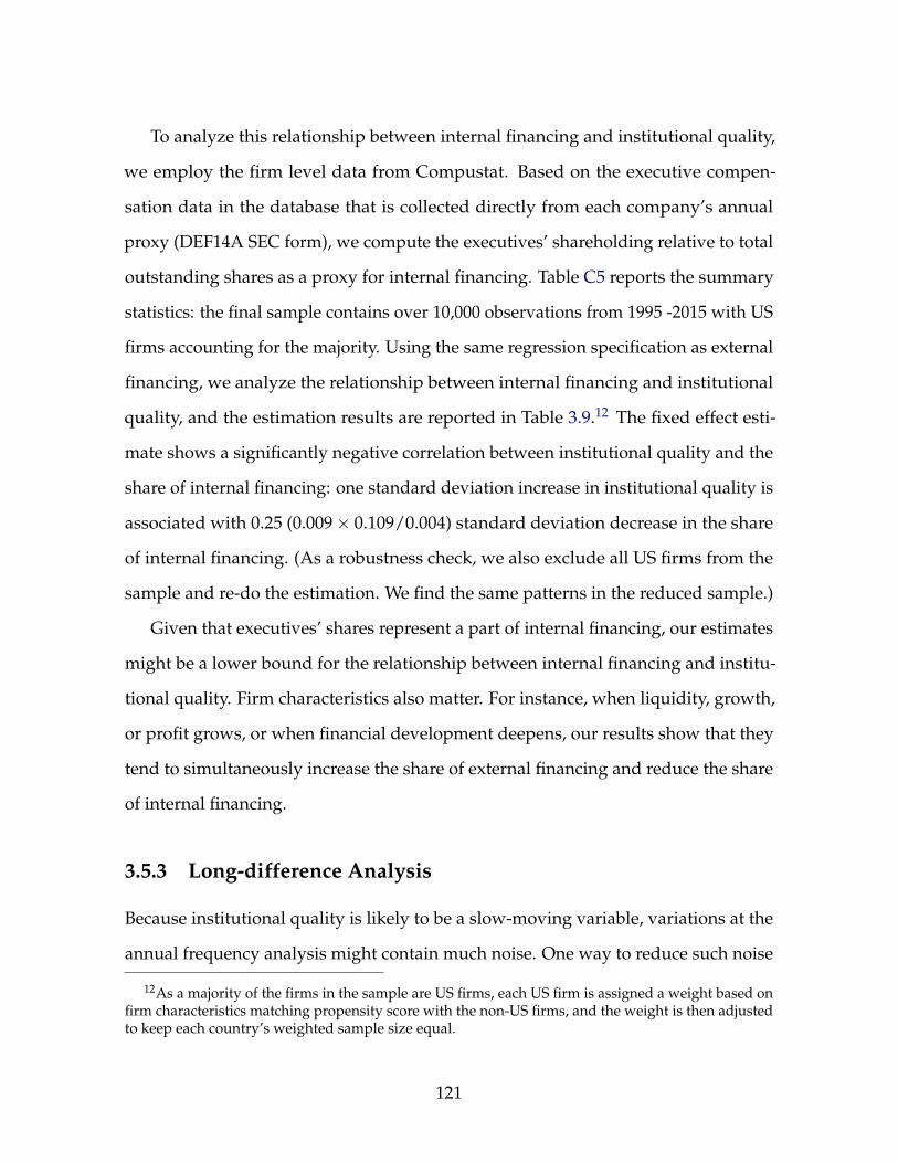
To analyze this relationship between internal financing and institutional quality,

we employ the firm level data from Compustat. Based on the executive compen-

sation data in the database that is collected directly from each company’s annual

proxy (DEF14A SEC form), we compute the executives’ shareholding relative to total

outstanding shares as a proxy for internal financing. Table C5 reports the summary

statistics: the final sample contains over 10,000 observations from 1995 -2015 with US

firms accounting for the majority. Using the same regression specification as external

financing, we analyze the relationship between internal financing and institutional

quality, and the estimation results are reported in Table 3.9.12 The fixed effect esti-

mate shows a significantly negative correlation between institutional quality and the

share of internal financing: one standard deviation increase in institutional quality is

associated with 0.25 (0.009× 0.109/0.004) standard deviation decrease in the share

of internal financing. (As a robustness check, we also exclude all US firms from the

sample and re-do the estimation. We find the same patterns in the reduced sample.)

Given that executives’ shares represent a part of internal financing, our estimates

might be a lower bound for the relationship between internal financing and institu-

tional quality. Firm characteristics also matter. For instance, when liquidity, growth,

or profit grows, or when financial development deepens, our results show that they

tend to simultaneously increase the share of external financing and reduce the share

of internal financing.

3.5.3 Long-difference Analysis

Because institutional quality is likely to be a slow-moving variable, variations at the

annual frequency analysis might contain much noise. One way to reduce such noise

12As a majority of the firms in the sample are US firms, each US firm is assigned a weight based onfirm characteristics matching propensity score with the non-US firms, and the weight is then adjustedto keep each country’s weighted sample size equal.

121

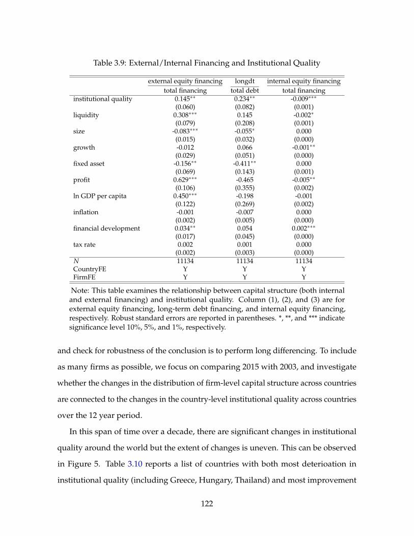
Table 3.9: External/Internal Financing and Institutional Quality

external equity financing longdt internal equity financingtotal financing total debt total financing

institutional quality 0.145∗∗ 0.234∗∗ -0.009∗∗∗

(0.060) (0.082) (0.001)liquidity 0.308∗∗∗ 0.145 -0.002∗

(0.079) (0.208) (0.001)size -0.083∗∗∗ -0.055∗ 0.000

(0.015) (0.032) (0.000)growth -0.012 0.066 -0.001∗∗

(0.029) (0.051) (0.000)fixed asset -0.156∗∗ -0.411∗∗ 0.000

(0.069) (0.143) (0.001)profit 0.629∗∗∗ -0.465 -0.005∗∗

(0.106) (0.355) (0.002)ln GDP per capita 0.450∗∗∗ -0.198 -0.001

(0.122) (0.269) (0.002)inflation -0.001 -0.007 0.000

(0.002) (0.005) (0.000)financial development 0.034∗∗ 0.054 0.002∗∗∗

(0.017) (0.045) (0.000)tax rate 0.002 0.001 0.000

(0.002) (0.003) (0.000)N 11134 11134 11134CountryFE Y Y YFirmFE Y Y Y

Note: This table examines the relationship between capital structure (both internaland external financing) and institutional quality. Column (1), (2), and (3) are forexternal equity financing, long-term debt financing, and internal equity financing,respectively. Robust standard errors are reported in parentheses. *, **, and *** indicatesignificance level 10%, 5%, and 1%, respectively.

and check for robustness of the conclusion is to perform long differencing. To include

as many firms as possible, we focus on comparing 2015 with 2003, and investigate

whether the changes in the distribution of firm-level capital structure across countries

are connected to the changes in the country-level institutional quality across countries

over the 12 year period.

In this span of time over a decade, there are significant changes in institutional

quality around the world but the extent of changes is uneven. This can be observed

in Figure 5. Table 3.10 reports a list of countries with both most deterioation in

institutional quality (including Greece, Hungary, Thailand) and most improvement

122

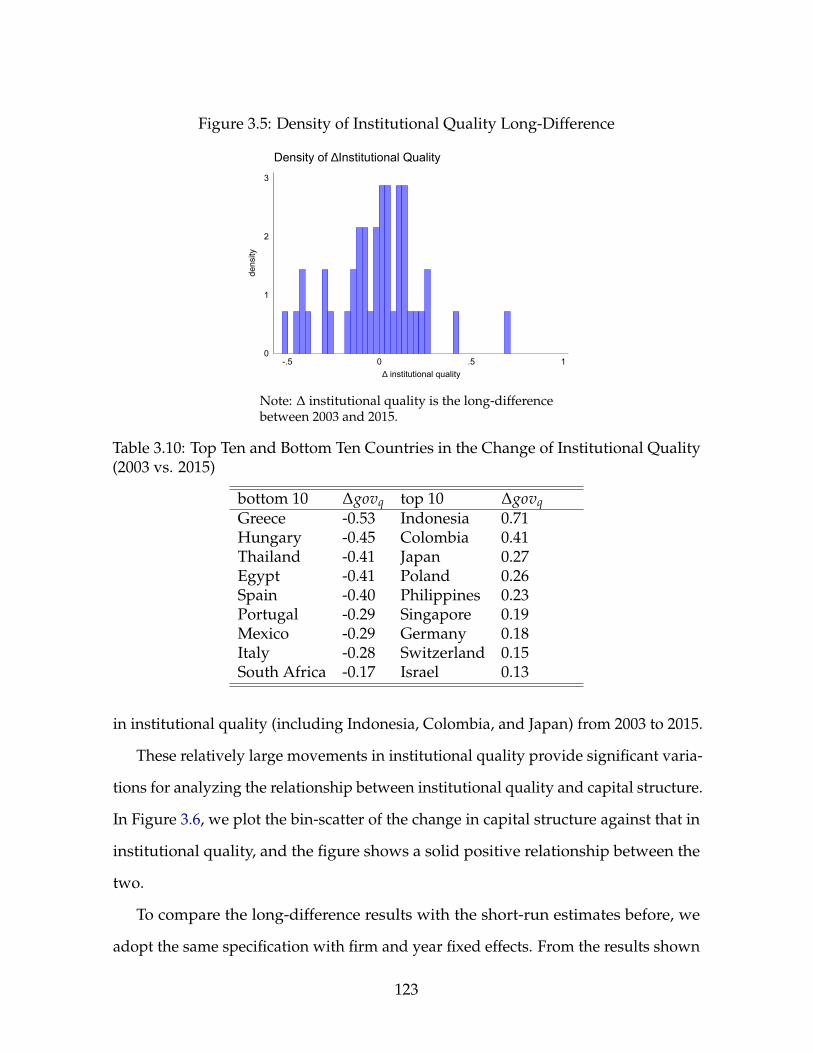
Figure 3.5: Density of Institutional Quality Long-Difference

0

1

2

3

dens

ity

-.5 0 .5 1∆ institutional quality

Density of ∆Institutional Quality

Note: ∆ institutional quality is the long-differencebetween 2003 and 2015.

Table 3.10: Top Ten and Bottom Ten Countries in the Change of Institutional Quality(2003 vs. 2015)

bottom 10 ∆govq top 10 ∆govqGreece -0.53 Indonesia 0.71Hungary -0.45 Colombia 0.41Thailand -0.41 Japan 0.27Egypt -0.41 Poland 0.26Spain -0.40 Philippines 0.23Portugal -0.29 Singapore 0.19Mexico -0.29 Germany 0.18Italy -0.28 Switzerland 0.15South Africa -0.17 Israel 0.13

in institutional quality (including Indonesia, Colombia, and Japan) from 2003 to 2015.

These relatively large movements in institutional quality provide significant varia-

tions for analyzing the relationship between institutional quality and capital structure.

In Figure 3.6, we plot the bin-scatter of the change in capital structure against that in

institutional quality, and the figure shows a solid positive relationship between the

two.

To compare the long-difference results with the short-run estimates before, we

adopt the same specification with firm and year fixed effects. From the results shown

123

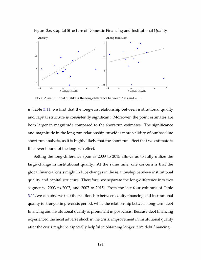
Figure 3.6: Capital Structure of Domestic Financing and Institutional Quality

-.05

0

.05

.1

-.4 -.2 0 .2 .4 .6∆ institutional quality

∆Equity

-.05

0

.05

.1

-.4 -.2 0 .2 .4 .6∆ institutional quality

∆Long-term Debt

Note: ∆ institutional quality is the long-difference between 2003 and 2015.

in Table 3.11, we find that the long-run relationship between institutional quality

and capital structure is consistently significant. Moreover, the point estimates are

both larger in magnitude compared to the short-run estimates. The significance

and magnitude in the long-run relationship provides more validity of our baseline

short-run analysis, as it is highly likely that the short-run effect that we estimate is

the lower bound of the long-run effect.

Setting the long-difference span as 2003 to 2015 allows us to fully utilize the

large change in institutional quality. At the same time, one concern is that the

global financial crisis might induce changes in the relationship between institutional

quality and capital structure. Therefore, we separate the long-difference into two

segments: 2003 to 2007, and 2007 to 2015. From the last four columns of Table

3.11, we can observe that the relationship between equity financing and institutional

quality is stronger in pre-crisis period, while the relationship between long-term debt

financing and institutional quality is prominent in post-crisis. Because debt financing

experienced the most adverse shock in the crisis, improvement in institutional quality

after the crisis might be especially helpful in obtaining longer term debt financing.

124

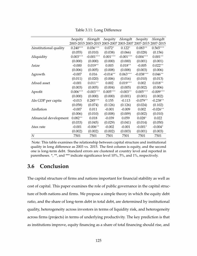
Table 3.11: Long Difference

∆equity ∆longdt ∆equity ∆longdt ∆equity ∆longdt2003-2015 2003-2015 2003-2007 2003-2007 2007-2015 2007-2015

∆institutional quality 0.240∗∗∗ 0.036∗∗∗ 0.072∗ 0.122∗ 0.083∗∗ 0.565∗∗∗

(0.055) (0.010) (0.038) (0.066) (0.028) (0.156)∆liquidity 0.003∗∗∗ -0.001∗∗∗ 0.001∗∗∗ -0.001∗∗∗ 0.004∗∗∗ 0.001∗∗

(0.000) (0.000) (0.000) (0.000) (0.001) (0.001)∆size -0.000 0.019∗∗ 0.003 0.018∗∗ -0.005 0.022∗∗

(0.006) (0.005) (0.008) (0.008) (0.003) (0.006)∆growth -0.007 0.016 -0.014∗∗ 0.063∗∗∗ -0.038∗∗∗ 0.046∗∗

(0.011) (0.020) (0.006) (0.016) (0.010) (0.013)∆fixed asset -0.001 0.011∗∗ 0.002 0.019∗∗∗ 0.002 0.018∗∗

(0.003) (0.005) (0.004) (0.005) (0.002) (0.006)∆profit 0.006∗∗∗ -0.003∗∗∗ 0.005∗∗∗ -0.003∗∗ 0.005∗∗∗ -0.009∗∗∗

(0.000) (0.000) (0.000) (0.001) (0.001) (0.002)∆ln GDP per capita -0.013 0.285∗∗∗ 0.155 -0.113 -0.079∗∗ -0.238∗∗

(0.058) (0.074) (0.126) (0.126) (0.024) (0.102)∆inflation -0.007 0.011 -0.001 -0.009 0.002 -0.026∗∗

(0.006) (0.010) (0.008) (0.009) (0.002) (0.010)∆financial development 0.082∗∗ 0.018 -0.039 0.059 0.028∗ 0.022

(0.033) (0.045) (0.029) (0.041) (0.014) (0.050)∆tax rate -0.001 -0.006∗∗ -0.002 -0.001 -0.001∗ -0.004∗

(0.002) (0.002) (0.002) (0.003) (0.001) (0.003)N 7501 7501 7501 7501 7501 7501

Note: This table examines the relationship between capital structure and institutionalquality in long difference as 2003 vs. 2015. The first column is equity, and the secondone is long-term debt. Standard errors are clustered at country level and reported inparentheses. *, **, and *** indicate significance level 10%, 5%, and 1%, respectively.

3.6 Conclusion

The capital structure of firms and nations important for financial stability as well as

cost of capital. This paper examines the role of public governance in the capital struc-

ture of both nations and firms. We propose a simple theory in which the equity debt

ratio, and the share of long-term debt in total debt, are determined by institutional

quality, heterogeneity across investors in terms of liquidity risk, and heterogeneity

across firms (projects) in terms of underlying productivity. The key prediction is that

as institutions improve, equity financing as a share of total financing should rise, and

125

long-term debt as a share of total debt should also rise.

We take these predictions to data on the structure of external liabilities (from

balance of payments) across countries, and find clear supportive evidence. We also

take the predictions to firm level data from Worldscope. We find that the cross-country

differences in the financing structure of firms depends on a country’s institutional

quality in ways that are consistent with the theory.

This paper documents the role of national institutions as an important common

determinant of the capital structure for all firms in a country and for the composition

of external liabilities of a country. Many extensions can be pursued. For example,

within debt, it might be useful to distinguish between loans from banks versus bonds

from the capital market. These are left for future research.

126

Bibliography

Aguiar, M. and Amador, M. (2013). Take the short route: How to repay and restructuresovereign debt with multiple maturities. Technical report, National Bureau ofEconomic Research.

Akıncı, Ö. (2013). Global financial conditions, country spreads and macroeconomicfluctuations in emerging countries. Journal of International Economics, 91(2):358–371.

Alesina, A. and Zhuravskaya, E. (2011). Segregation and the quality of governmentin a cross section of countries. The American Economic Review, 101(5):1872–1911.

Alfaro, L., Kalemli-Ozcan, S., and Volosovych, V. (2008). Why doesn’t capital flowfrom rich to poor countries? an empirical investigation. The Review of Economicsand Statistics, 90(2):347–368.

Alfaro, L. and Kanczuk, F. (2009). Debt maturity: Is long-term debt optimal? Reviewof international Economics, 17(5):890–905.

Ang, A. and Piazzesi, M. (2003). A no-arbitrage vector autoregression of term structuredynamics with macroeconomic and latent variables. Journal of Monetary economics,50(4):745–787.

Arellano, C. and Ramanarayanan, A. (2012). Default and the maturity structure insovereign bonds. Journal of Political Economy, 120(2):187–232.

Benigno, G., Chen, H., Otrok, C., Rebucci, A., and Young, E. R. (2013). Financial crisesand macro-prudential policies. Journal of International Economics, 89(2):453–470.

Benigno, G., Chen, H., Otrok, C., Rebucci, A., and Young, E. R. (2016a). Optimalcapital controls and real exchange rate policies: A pecuniary externality perspective.Journal of Monetary Economics, 84:147–165.

Benigno, G., Chen, H., Otrok, C., Rebucci, A., and Young, E. R. (2016b). Optimalcapital controls and real exchange rate policies: A pecuniary externality perspective.Journal of Monetary Economics, 84:147–165.

Bianchi, J. (2011a). Overborrowing and systemic externalities in the business cycle.The American Economic Review, 101(7):3400–3426.

Bianchi, J. (2011b). Overborrowing and systemic externalities in the business cycle.American Economic Review, 101(7):3400–3426.

127

Bianchi, J., Hatchondo, J. C., and Martinez, L. (2012). International reserves androllover risk. Technical report, National Bureau of Economic Research.

Bianchi, J. and Mendoza, E. G. (2013). Optimal time-consistent macroprudentialpolicy. Technical report, National Bureau of Economic Research.

Bluedorn, J. C., Duttagupta, R., Guajardo, J., and Topalova, P. B. (2013). Capital flowsare fickle: Anytime, anywhere. IMF Staff Papers, (183).

Bocola, L. and Dovis, A. (2016). Self-fulfilling debt crises: A quantitative analysis.Technical report, National Bureau of Economic Research.

Bolton, P. and Huang, H. (2016). The capital structure of nations. Mimeo.

Bolton, P. and Scharfstein, D. S. (1996). Optimal debt structure and the number ofcreditors. Journal of Political Economy, 104(1):1–25.

Broner, F., Didier, T., Erce, A., and Schmukler, S. L. (2013a). Gross capital flows:Dynamics and crises. Journal of Monetary Economics, 60(1):113–133.

Broner, F. A., Lorenzoni, G., and Schmukler, S. L. (2013b). Why do emergingeconomies borrow short term? Journal of the European Economic Association,11(suppl_1):67–100.

Brunnermeier, M. K. (2009). Deciphering the liquidity and credit crunch 2007–2008.The Journal of economic perspectives, 23(1):77–100.

Brunnermeier, M. K. and Oehmke, M. (2013). The maturity rat race. The Journal ofFinance, 68(2):483–521.

Brunnermeier, M. K. and Yogo, M. (2009). A note on liquidity risk management.American Economic Review, 99(2):578–83.

Chang, R. and Fernández, A. (2013). On the sources of aggregate fluctuations inemerging economies. International Economic Review, 54(4):1265–1293.

Chang, R., Fernández, A., and Gulan, A. (2017). Bond finance, bank credit, andaggregate fluctuations in an open economy. Journal of Monetary Economics, 85:90–109.

Chatterjee, S. and Eyigungor, B. (2012). Maturity, indebtedness, and default risk. TheAmerican Economic Review, 102(6):2674–2699.

Claessens, S., Tong, H., and Wei, S.-J. (2012). From the financial crisis to the real econ-omy: Using firm-level data to identify transmission channels. Journal of InternationalEconomics, 88(2):375–387.

Cole, H. L. and Kehoe, T. J. (2000). Self-fulfilling debt crises. The Review of EconomicStudies, 67(1):91–116.

128

Contessi, S., De Pace, P., and Francis, J. L. (2013). The cyclical properties of disaggre-gated capital flows. Journal of International Money and Finance, 32:528–555.

Crouzet, N. (2014). Aggregate implications of corporate debt choices. Mimeo.

De Fiore, F. and Uhlig, H. (2015). Corporate debt structure and the financial crisis.Journal of Money, credit and Banking, 47(8):1571–1598.

Devereux, M. B., Young, E. R., and Yu, C. (2015). A new dilemma: Capital controlsand monetary policy in sudden stop economies. Technical report, National Bureauof Economic Research.

Eichengreen, B., Gupta, P., and Masetti, O. (2017). Are capital flows fickle? increas-ingly? and does the answer still depend on type? Policy Research working paper,WPS7972.

Epstein, G. A. and Schor, J. B. (1989). Structural determinants and economic effects ofcapital controls in the OECD. Harvard Institute of Economic Research, HarvardUniversity.

Evans, M. and Hnatkovska, V. V. (2014). International capital flows, returns andworld financial integration. Journal of International Economics, 92(1):14–33.

Farhi, E. and Tirole, J. (2012). Collective moral hazard, maturity mismatch, andsystemic bailouts. The American Economic Review, 102(1):60–93.

Faria, A. and Mauro, P. (2009). Institutions and the external capital structure ofcountries. Journal of International Money and Finance, 28(3):367–391.

Federico, P., Vegh, C. A., and Vuletin, G. (2014). Reserve requirement policy over thebusiness cycle. Technical report, National Bureau of Economic Research.

Fernández, A., Klein, M. W., Rebucci, A., Schindler, M., and Uribe, M. (2016a). Capitalcontrol measures: A new dataset. IMF Economic Review, 64(3):548–574.

Fernández, A., Klein, M. W., Rebucci, A., Schindler, M., and Uribe, M. (2016b). Capitalcontrol measures: A new dataset. IMF Economic Review, 64(3):548–574.

Fernández, A., Rebucci, A., and Uribe, M. (2015a). Are capital controls countercyclical?Journal of Monetary Economics, 76:1–14.

Fernández, A., Rebucci, A., and Uribe, M. (2015b). Are capital controls countercyclical?Journal of Monetary Economics, 76:1–14.

Forbes, K., Reinhardt, D., and Wieladek, T. (2017). The spillovers, interactions, and(un) intended consequences of monetary and regulatory policies. Journal of MonetaryEconomics, 85:1–22.

129

Frank, M. Z. and Goyal, V. K. (2003). Testing the pecking order theory of capitalstructure. Journal of financial economics, 67(2):217–248.

Frank, M. Z. and Goyal, V. K. (2009). Capital structure decisions: which factors arereliably important? Financial management, 38(1):1–37.

Fratzscher, M. (2012). Capital flows, push versus pull factors and the global financialcrisis. Journal of International Economics, 88(2):341–356.

Gelos, R. G. and Wei, S.-J. (2002). Transparency and international investor behavior.Technical report, National Bureau of Economic Research.

Goldstein, I. and Razin, A. (2006). An information-based trade off between foreigndirect investment and foreign portfolio investment. Journal of International Economics,70(1):271–295.

Gomes, J., Jermann, U., and Schmid, L. (2016). Sticky leverage. American EconomicReview, 106(12):3800–3828.

Gourinchas, P.-O., Valdes, R., and Landerretche, O. (2001). Lending booms: Latinamerica and the world. Technical report, National Bureau of Economic Research.

Hatchondo, J. C. and Martinez, L. (2009). Long-duration bonds and sovereign defaults.Journal of international Economics, 79(1):117–125.

He, Z. and Xiong, W. (2012). Dynamic debt runs. The Review of Financial Studies,25(6):1799–1843.

Hennessy, C. A. and Whited, T. M. (2007). How costly is external financing? evidencefrom a structural estimation. The Journal of Finance, 62(4):1705–1745.

Ilzetzki, E., Reinhart, C. M., and Rogoff, K. S. (2011). The country chronologies andbackground material to exchange rate arrangements into the 21st century: Will theanchor currency hold. manuscript.

Jeanne, O. (2009). Debt maturity and the international financial architecture. TheAmerican Economic Review, 99(5):2135–2148.

Jeanne, O. and Korinek, A. (2010). Managing credit booms and busts: A pigouviantaxation approach. Technical report, National Bureau of Economic Research.

Kalemli-Ozcan, S., Sorensen, B., and Yesiltas, S. (2012). Leverage across firms, banks,and countries. Journal of international Economics, 88(2):284–298.

Kaplan, S. N. and Zingales, L. (1997). Do investment-cash flow sensitivities pro-vide useful measures of financing constraints? The quarterly journal of economics,112(1):169–215.

130

Kastner, S. L. and Rector, C. (2003). International regimes, domestic veto-players, andcapital controls policy stability. International Studies Quarterly, 47(1):1–22.

Klein, M. W. (2005). Capital account liberalization, institutional quality and economicgrowth: theory and evidence. Technical report, National Bureau of EconomicResearch.

Klein, M. W. (2012). Capital controls: Gates versus walls. Brookings Papers on EconomicActivity, pages 317–367.

Korinek, A. (2010). Regulating capital flows to emerging markets: An externalityview. manuscript.

Korinek, A. (2017). Regulating capital flows to emerging markets: An externalityview. Journal of International Economics, forthcoming.

Laeven, L. and Valencia, F. (2013). Systemic banking crises database. IMF EconomicReview, 61(2):225–270.

Lane, P. R. and Milesi-Ferretti, G. M. (2007). The external wealth of nations mark ii:Revised and extended estimates of foreign assets and liabilities, 1970–2004. Journalof international Economics, 73(2):223–250.

Levchenko, A. A. and Mauro, P. (2007). Do some forms of financial flows help protectagainst sudden stops? The World Bank Economic Review, 21(3):389–411.

Lyandres, E. (2007). Costly external financing, investment timing, and investment–cash flow sensitivity. Journal of Corporate Finance, 13(5):959–980.

Mendoza, E. G. (2010). Sudden stops, financial crises, and leverage. The AmericanEconomic Review, 100(5):1941–1966.

Mendoza, E. G. and Smith, K. A. (2006). Quantitative implications of a debt-deflationtheory of sudden stops and asset prices. Journal of International Economics, 70(1):82–114.

Mendoza, E. G. and Terrones, M. E. (2008). An anatomy of credit booms: evidencefrom macro aggregates and micro data. Technical report, National Bureau ofEconomic Research.

Miao, J. and Wang, P. (2010). Credit risk and business cycles. working paper.

Mukherjee, R. (2015). Institutions, corporate governance and capital flows. Journal ofInternational Economics, 96(2):338–359.

Myers, S. C. and Majluf, N. S. (1984). Corporate financing and investment deci-sions when firms have information that investors do not have. Journal of financialeconomics, 13(2):187–221.

131

Na, S., Schmitt-Grohé, S., Uribe, M., and Yue, V. Z. (2014a). A model of the twin ds:Optimal default and devaluation. Technical report, National Bureau of EconomicResearch.

Na, S., Schmitt-Grohé, S., Uribe, M., and Yue, V. Z. (2014b). A model of the twinds: Optimal default and devaluation. Working Paper 20314, National Bureau ofEconomic Research.

Neumeyer, P. A. and Perri, F. (2005). Business cycles in emerging economies: the roleof interest rates. Journal of monetary Economics, 52(2):345–380.

Opler, T., Pinkowitz, L., Stulz, R., and Williamson, R. (1999). The determinants andimplications of corporate cash holdings. Journal of financial economics, 52(1):3–46.

Ostry, J. D., Ghosh, A. R., Habermeier, K., Chamon, M., Qureshi, M. S., and Reinhardt,D. (2010). Capital inflows: The role of controls. Revista de Economia Institucional,12(23):135–164.

Pasricha, G., Falagiarda, M., Bijsterbosch, M., and Aizenman, J. (2015). Domestic andmultilateral effects of capital controls in emerging markets. Working Paper 20822,National Bureau of Economic Research.

Qian, J. and Strahan, P. E. (2007). How laws and institutions shape financial contracts:The case of bank loans. The Journal of Finance, 62(6):2803–2834.

Quinn, D. (1997). The correlates of change in international financial regulation.American Political science review, 91(03):531–551.

Quinn, D., Schindler, M., and Toyoda, A. M. (2011a). Assessing measures of financialopenness and integration. IMF Economic Review, 59(3):488–522.

Quinn, D., Schindler, M., and Toyoda, A. M. (2011b). Assessing measures of financialopenness and integration. IMF Economic Review, 59(3):488–522.

Rajan, R. G. and Zingales, L. (1995). What do we know about capital structure? someevidence from international data. The journal of Finance, 50(5):1421–1460.

Razin, A., Sadka, E., and Yuen, C.-W. (1998). A pecking order of capital inflows andinternational tax principles. Journal of International Economics, 44(1):45–68.

Rey, H. (2015). Dilemma not trilemma: the global financial cycle and monetary policyindependence. Technical report, National Bureau of Economic Research.

Rogoff, K. S. and Reinhart, C. M. (2009). The aftermath of financial crises. NationalBureau of Economic Research.

Schindler, M. (2009). Measuring financial integration: A new data set. IMF StaffPapers, 56(1):222–238.

132

Schmitt-Grohé, S. and Uribe, M. (2016). Downward nominal wage rigidity, currencypegs, and involuntary unemployment. Journal of Political Economy, 124(5):1466–1514.

Schmitt-Grohé, S. and Uribe, M. (2016). Is optimal capital-control policy countercycli-cal in open-economy models with collateral constraints? Working Paper 22481,National Bureau of Economic Research.

Schmitt-Grohé, S. and Uribe, M. (2016). Multiple equilibria in open economy modelswith collateral constraints: Overborrowing revisited.

Schmitt-Grohé, S. and Uribe, M. (2017). Is optimal capital control policy countercycli-cal in open economy models with collateral constraints? IMF Economic Review,65(3):498–527.

Shleifer, A. and Vishny, R. W. (1997). A survey of corporate governance. The journal offinance, 52(2):737–783.

Tong, H. and Wei, S.-J. (2010). The composition matters: capital inflows and liquiditycrunch during a global economic crisis. The Review of Financial Studies, 24(6):2023–2052.

Uribe, M. and Yue, V. Z. (2006). Country spreads and emerging countries: Who driveswhom? Journal of international Economics, 69(1):6–36.

133

Appendix to Chapter 1

134

Procedure for Constructing Index of Changes in CapitalControlBased on AREAER, the construction of changes in capital controls takes the followingsteps.

1. Extract the narratives of policies regarding capital transaction in the “Changesin the previous year” at the end of country profile from AREAER.Post-1998 years are directly downloaded from AREAER website. From 1983to 1998 is extracted manually from each AREAER. Prior to 1983, the policiesare listed in the chronological manner without indicating whether it is aboutcapital transaction or not. Therefore, discretion is used for the selection.

2. Extract the maturity-related policies.First, search for the policies whose narratives contain “day”, “week”, “month”,“quarter”, “year”, “short”, and “long”. Second, label whether it targets short-term (intending to lengthening the average maturity) or long-term (intendingto shortening the average maturity).

3. Each policy is characterized by three labels: the direction of transaction, whetherit is a tightening or easing, whether it is associated with short-term, or long-term,or independent.

135

Proof of Proposition 1The regulated competitive equilibrium is defined as

maxcT

t ,cNt ,dS

t+1,dLt+1, ft,τS

t ,τLt

E0

∞

∑0

βtU(cTt , cN

t )

s.t. U′Tt = λt (6)

pt =1− α

α

( cTt

cNt

)1/ξ(7)

λt[(1− τS

t )qSt − µt

]= βEtλt+1 (8)

λt[(1− τL

t )qLt − µt

]= βEt

[λt+1

(1 + δ(1− τL

t+1)qLt+1)]

(9)

µt ≥ 0 (10)

µt[κ((1− γ) f γ

t + ptyNt)− dS

t+1 − dLt+1]= 0 (11)

dSt+1 + dL

t+1 ≤ κ[Γ(1− γ) f γ

t + ptyNt]

(12)

cNt = yN

t (13)

cTt + dS

t + dLt = Γ(1− γ) f γ

t + qSt dS

t+1 + qLt (d

Lt+1 − δdL

t )(14)

Γγ f γ−1t = 1 + (

1qS

t− 1)η (15)

Lemma 1. Any process {cTt , dS

t+1, dLt+1} satisfy (A.1) to (A.10) if and only if they satisfy

(A.9), (A.10), and

dSt+1 + dL

t+1 ≤ κ[Γ(1− γ) f γ

t +1− α

α

( cTt

cNt

)1/ξyN

t

](16)

Proof. From (A.9) - (A.11) to (A.1) - (A.10):From cT

t , cNt , we can define λt using (A.1) and pt using (A.2). Then, we set µ = 0

which validates (A.5) and (A.6), and we choose τSt , τL

t according to (A.3) and (A.4).With pt satisfying (A.2), (A.7) is equivalent to (A.11).From (A.1) - (A.10) to (A.9) - (A.11): plugging (A.2) to (A.7) yields (A.11).

Lemma 1 suggests that the regulated competitive equilibrium is equivalent to Ram-sey equilibrium with properly defined taxes, which essentially proves that Ramseyequilibrium can be decentralized.

136

Proof of Proposition 2Proof. Suppose that the collateral constraint does not bind, then the correspondingEuler equations for short- and long-term debt are

qSt = Et

βu′t+1U′t

qLt = E

[βu′t+1u′t

(1 + δqL

t+1)]

= Etβu′t+1

u′tEt(1 + δqL

t+1)+ δCov

(βU′t+1U′t

, qLt+1)

= qSt Et(1 + δqL

t+1)+ δCov

(βu′t+1u′t

, qLt+1)

With risk-neutral foreign investor, the long-term debt’s price is associated with theprice of the short-term.

qLt = qS

t Et(1 + δqL

t+1)

Therefore, if the covariance term is positive13, there will not be long-term debt,otherwise, there will not be short-term debt.

Ruling Out Multiple EquilibriaSchmitt-Grohe and Uribe (2016) show that under plausible calibrations, there existmultiple equilibria with both underborrowing and overborrowing. Multiple equilib-ria stem from a self-fullfiling decline in nontradable goods price leading to reductionin collateral value, consumption, and nontradable goods price in a compatible feed-back loop. Specifically, when collateral constraint binds, tradable goods consumptionis pinned down by the collateral value which hinges on the level of consumptionitself.

cTt = κ

[yT

t + yNt

1− α

α

( cTt

cNt

)1/ξ]≡ f (cT

t ) (17)

As discussed in Jeanne and Korinek (2012) and Benigno et al. (2016), when the elastic-ity of substitution between tradable and nontradable goods is less than one, a suffi-cient condition of unique equilibrium requires limcT

t →0 f ′(cTt ) = 0, limcT

t →∞ f ′(cTt ) =

∞, and f ′(cTt )∣∣cT

t = f (cTt )

> 1. These conditions are satisfied in the calibration.Intuitively, given tradable and nontradable goods are complements, when extra

borrowing increases tradable consumption, nontradable consumption will rise si-multaneously. As a result, nontradable price goes up, so will collateral value andborrowing limit. If they are substitutes, then borrowing increase will lead to nontrad-able consumption decrease and reduce borrowing limit.

13In the case without interest rate shock, the covariance term is zero, so the maturity structure isundetermined.

137

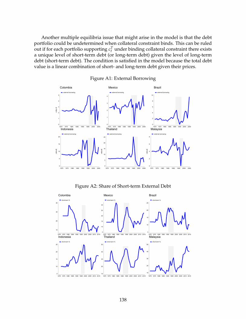
Another multiple equilibria issue that might arise in the model is that the debtportfolio could be undetermined when collateral constraint binds. This can be ruledout if for each portfolio supporting cT

t under binding collateral constraint there existsa unique level of short-term debt (or long-term debt) given the level of long-termdebt (short-term debt). The condition is satisfied in the model because the total debtvalue is a linear combination of short- and long-term debt given their prices.

Figure A1: External Borrowing

0

1

2

3

4

5

milli

on $

1970 1975 1980 1985 1990 1995 2000 2005

external borrowing

Colombia

0

1

2

3

4

1970 1975 1980 1985 1990 1995 2000 2005

external borrowing

Mexico

0

2

4

6

8

10

1970 1975 1980 1985 1990 1995 2000 2005

external borrowing

Brazil

0

5

10

15

20

milli

on$

1970 1975 1980 1985 1990 1995 2000 2005

external borrowing

Indonesia

0

5

10

15

20

25

milli

on$

1970 1975 1980 1985 1990 1995 2000 2005

external borrowing

Thailand

0

2

4

6

8

milli

on$

1970 1975 1980 1985 1990 1995 2000 2005

external borrowing

Malaysia

Figure A2: Share of Short-term External Debt

10

20

30

40

1970 1975 1980 1985 1990 1995 2000 2005 2010 2015

short-term %

Colombia

5

10

15

20

25

30

1970 1975 1980 1985 1990 1995 2000 2005 2010 2015

short-term %

Mexico

5

10

15

20

25

1970 1975 1980 1985 1990 1995 2000 2005 2010 2015

short-term %

Brazil

5

10

15

20

25

1970 1975 1980 1985 1990 1995 2000 2005 2010 2015

short-term %

Indonesia

10

20

30

40

50

1970 1975 1980 1985 1990 1995 2000 2005 2010 2015

short-term %

Thailand

10

20

30

40

50

1970 1975 1980 1985 1990 1995 2000 2005 2010 2015

short-term %

Malaysia

138

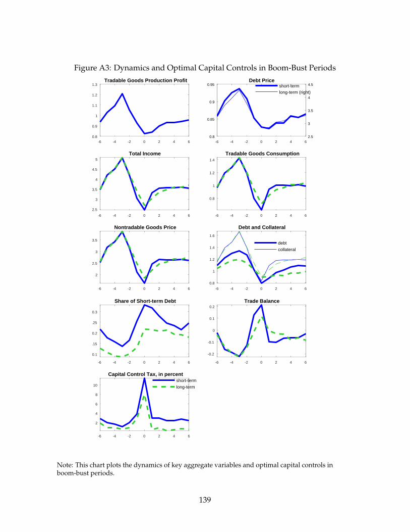
Figure A3: Dynamics and Optimal Capital Controls in Boom-Bust Periods

-6 -4 -2 0 2 4 60.8

0.9

1

1.1

1.2

1.3Tradable Goods Production Profit

-6 -4 -2 0 2 4 60.8

0.85

0.9

0.95

2.5

3

3.5

4

4.5Debt Price

short-termlong-term (right)

-6 -4 -2 0 2 4 6

2.5

3

3.5

4

4.5

5

Total Income

-6 -4 -2 0 2 4 6

0.8

1

1.2

1.4


-6 -4 -2 0 2 4 6

2

2.5

3

3.5


-6 -4 -2 0 2 4 6

0.8

1

1.2

1.4

1.6

Debt and Collateral

debt

collateral

-6 -4 -2 0 2 4 6

0.1

0.15

0.2

0.25

0.3


-6 -4 -2 0 2 4 6

-0.2

-0.1

0

0.1

0.2Trade Balance

-6 -4 -2 0 2 4 6

2

4

6

8

10

Capital Control Tax, in percentshort-term

long-term

Note: This chart plots the dynamics of key aggregate variables and optimal capital controls inboom-bust periods.

139

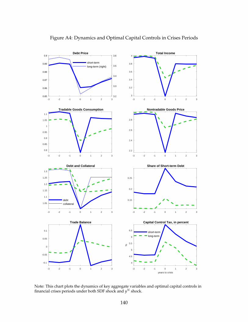
Figure A4: Dynamics and Optimal Capital Controls in Crises Periods

-3 -2 -1 0 1 2 30.85

0.86

0.87

0.88

0.89

0.9

3.2

3.3

3.4

3.5

3.6Debt Price

short-term

long-term (right)

-3 -2 -1 0 1 2 3

3

3.2

3.4

3.6

3.8

4Total Income

-3 -2 -1 0 1 2 3

0.8

0.85

0.9

0.95

1

1.05

1.1


-3 -2 -1 0 1 2 3

2.2

2.4

2.6

2.8


-3 -2 -1 0 1 2 3

1.05

1.1

1.15

1.2

1.25

1.3

Debt and Collateral

debtcollateral

-3 -2 -1 0 1 2 3

0.15

0.2

0.25


-3 -2 -1 0 1 2 3

-0.1

-0.05

0

0.05

0.1

Trade Balance

-3 -2 -1 0 1 2 3

years to crisis

4

4.5

5

5.5

6

6.5

%


short-term

long-term

Note: This chart plots the dynamics of key aggregate variables and optimal capital controls infinancial crises periods under both SDF shock and yN shock.

140


141

Categorization of Transaction and FlowsFrom Compilation Guide, AREAER 2012.

• Capital market instrument: shares and other securities of a participating natureand bonds and other securities with an original maturity of more than one year.

• Money market instrument: securities with an original maturity of one year orless and includes short-term instruments, such as certificates of deposit andbills of exchange. The category also includes treasury bills and other short-termgovernment paper, bankers’ acceptances, commercial paper, interbank deposits,and repurchase agreements.

• Derivatives: operations in other negotiable instruments and nonsecured claimsnot covered under the above subsections. These may include operations inrights; warrants; financial options and futures; secondary market operations inother financial claims (including sovereign loans, mortgage loans, commercialcredits, negotiable instruments originating as loans, receivables, and discountedbills of trade); forward operations (including those in foreign exchange); swapsof bonds and other debt securities; credits and loans; and other swaps (e.g.,interest rate, debt/equity, equity/debt, foreign currency, and swaps of any ofthe instruments listed above). Also included are operations in foreign exchangewithout any other underlying transaction (spot or forward trading on the foreignexchange markets, forward cover operations, etc.).

• Credit transaction: operations directly linked with international trade trans-actions or with the rendering of international services.. Credits other thancommercial credits granted by all residents, including banks, to nonresidents,or vice versa. Guarantees, sureties, and financial backup facilities provided byresidents to nonresidents and vice versa. It also includes securities pledged forpayment or performance of a contract such as warrants, performance bonds, andstandby letters of credit and financial backup facilities that are credit facilitiesused as a guarantee for independent financial operations.

• FDI: investments for the purpose of establishing lasting economic relations bothabroad by residents and domestically by nonresidents. These investments areessentially for the purpose of producing goods and services, and, in particular,in order to allow investor participation in the management of an enterprise.The category includes the creation or extension of a wholly owned enterprise,subsidiary, or branch and the acquisition of full or partial ownership of a newor existing enterprise that results in effective influence over the operations ofthe enterprise.

142

The Procedure of Constructing Measures of CapitalControl from "Changes" SectionThe construction takes the following steps.

1. Extract the narratives of policies regarding capital transaction in the "Changesin the previous year" at the end of country profile from AREAER.Post-1998 years are directly downloaded from AREAER website. From 1983to 1998 is extracted manually from each AREAER. Prior to 1983, the policiesare listed in the chronological manner without indicating whether it is aboutcapital transaction or not. Therefore, discretion is used for the selection.

2. Each policy is characterized by three labels: the type of transaction, the directionof transaction, whether it is a tightening or easing.Transaction types: FDI; credit transaction; capital market instrument/moneymarket instrument/financial derivativesDirection types: inflow; outflow

3. Extract the maturity-related policies.First, search for the policies whose narratives contain "day", "week", "month","quarter", "year", "short", and "long". Second, label whether it targets short-term(intending to lengthening the average maturity) or long-term (intending toshortening the average maturity).

143


144

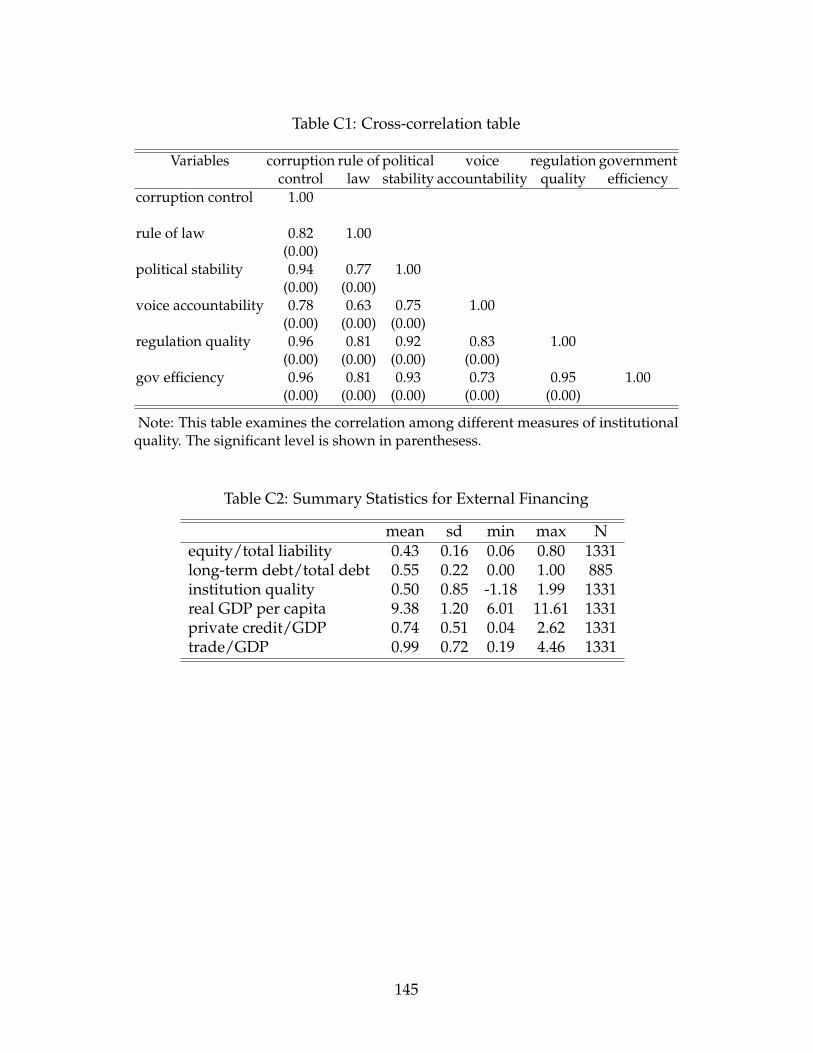
Table C1: Cross-correlation table

Variables corruption rule of political voice regulation governmentcontrol law stability accountability quality efficiency

corruption control 1.00

rule of law 0.82 1.00(0.00)

political stability 0.94 0.77 1.00(0.00) (0.00)

voice accountability 0.78 0.63 0.75 1.00(0.00) (0.00) (0.00)

regulation quality 0.96 0.81 0.92 0.83 1.00(0.00) (0.00) (0.00) (0.00)

gov efficiency 0.96 0.81 0.93 0.73 0.95 1.00(0.00) (0.00) (0.00) (0.00) (0.00)

Note: This table examines the correlation among different measures of institutionalquality. The significant level is shown in parenthesess.

Table C2: Summary Statistics for External Financing

mean sd min max Nequity/total liability 0.43 0.16 0.06 0.80 1331long-term debt/total debt 0.55 0.22 0.00 1.00 885institution quality 0.50 0.85 -1.18 1.99 1331real GDP per capita 9.38 1.20 6.01 11.61 1331private credit/GDP 0.74 0.51 0.04 2.62 1331trade/GDP 0.99 0.72 0.19 4.46 1331

145

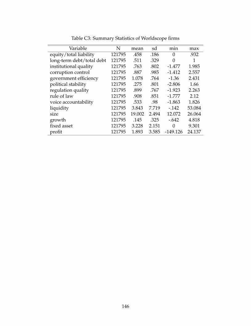
Table C3: Summary Statistics of Worldscope firms

Variable N mean sd min maxequity/total liability 121795 .458 .186 0 .932long-term debt/total debt 121795 .511 .329 0 1institutional quality 121795 .763 .802 -1.477 1.985corruption control 121795 .887 .985 -1.412 2.557government efficiency 121795 1.078 .764 -1.36 2.431political stability 121795 .275 .801 -2.806 1.66regulation quality 121795 .899 .767 -1.923 2.263rule of law 121795 .908 .851 -1.777 2.12voice accountability 121795 .533 .98 -1.863 1.826liquidity 121795 3.843 7.719 -.142 53.084size 121795 19.002 2.494 12.072 26.064growth 121795 .145 .325 -.642 4.818fixed asset 121795 3.228 2.151 0 9.301profit 121795 1.893 3.585 -149.126 24.137

146

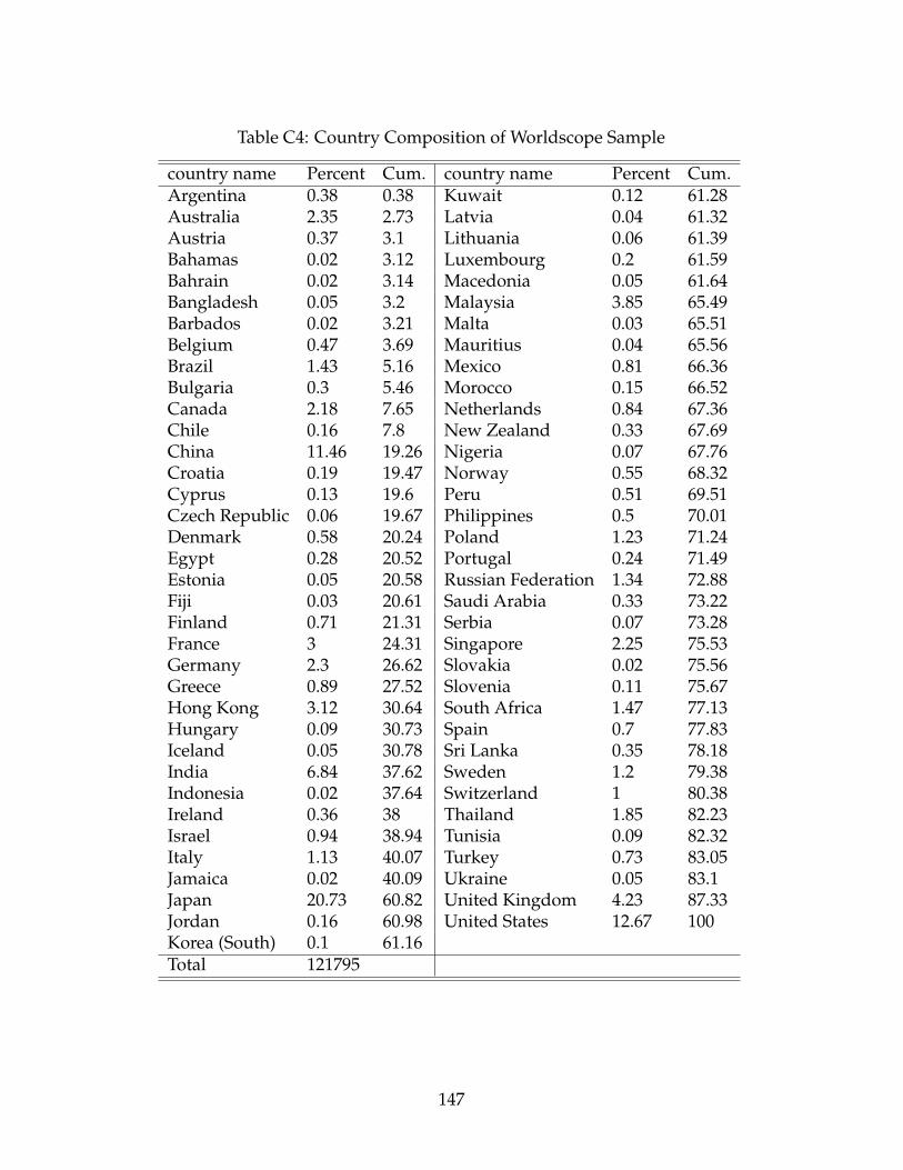
Table C4: Country Composition of Worldscope Sample

country name Percent Cum. country name Percent Cum.Argentina 0.38 0.38 Kuwait 0.12 61.28Australia 2.35 2.73 Latvia 0.04 61.32Austria 0.37 3.1 Lithuania 0.06 61.39Bahamas 0.02 3.12 Luxembourg 0.2 61.59Bahrain 0.02 3.14 Macedonia 0.05 61.64Bangladesh 0.05 3.2 Malaysia 3.85 65.49Barbados 0.02 3.21 Malta 0.03 65.51Belgium 0.47 3.69 Mauritius 0.04 65.56Brazil 1.43 5.16 Mexico 0.81 66.36Bulgaria 0.3 5.46 Morocco 0.15 66.52Canada 2.18 7.65 Netherlands 0.84 67.36Chile 0.16 7.8 New Zealand 0.33 67.69China 11.46 19.26 Nigeria 0.07 67.76Croatia 0.19 19.47 Norway 0.55 68.32Cyprus 0.13 19.6 Peru 0.51 69.51Czech Republic 0.06 19.67 Philippines 0.5 70.01Denmark 0.58 20.24 Poland 1.23 71.24Egypt 0.28 20.52 Portugal 0.24 71.49Estonia 0.05 20.58 Russian Federation 1.34 72.88Fiji 0.03 20.61 Saudi Arabia 0.33 73.22Finland 0.71 21.31 Serbia 0.07 73.28France 3 24.31 Singapore 2.25 75.53Germany 2.3 26.62 Slovakia 0.02 75.56Greece 0.89 27.52 Slovenia 0.11 75.67Hong Kong 3.12 30.64 South Africa 1.47 77.13Hungary 0.09 30.73 Spain 0.7 77.83Iceland 0.05 30.78 Sri Lanka 0.35 78.18India 6.84 37.62 Sweden 1.2 79.38Indonesia 0.02 37.64 Switzerland 1 80.38Ireland 0.36 38 Thailand 1.85 82.23Israel 0.94 38.94 Tunisia 0.09 82.32Italy 1.13 40.07 Turkey 0.73 83.05Jamaica 0.02 40.09 Ukraine 0.05 83.1Japan 20.73 60.82 United Kingdom 4.23 87.33Jordan 0.16 60.98 United States 12.67 100Korea (South) 0.1 61.16Total 121795

147

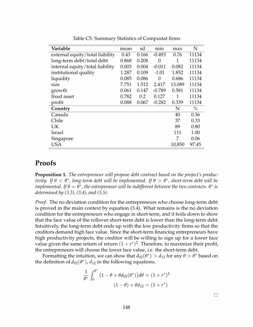
Table C5: Summary Statistics of Compustat firms

Variable mean sd min max Nexternal equity/total liability 0.43 0.166 -0.493 0.76 11134long-term debt/total debt 0.868 0.208 0 1 11134internal equity/total liability 0.003 0.004 -0.011 0.082 11134institutional quality 1.287 0.109 -1.01 1.852 11134liquidity 0.085 0.086 0 0.686 11134size 7.751 1.512 2.417 13.089 11134growth 0.061 0.147 -0.789 0.581 11134fixed asset 0.782 0.2 0.127 1 11134profit 0.088 0.067 -0.282 0.339 11134Country N %Canada 40 0.36Chile 37 0.33UK 89 0.80Israel 111 1.00Singapore 7 0.06USA 10,850 97.45

ProofsProposition 1. The entrepreneur will propose debt contract based on the project’s produc-tivity. If θ < θ∗, long-term debt will be implemented. If θ > θ∗, short-term debt will beimplemented. If θ = θ∗, the entrepreneur will be indifferent between the two contracts. θ∗ isdetermined by (3.3), (3.4), and (3.5).

Proof. The no deviation condition for the entrepreneurs who choose long-term debtis proved in the main context by equation (3.4). What remains is the no deviationcondition for the entrepreneurs who engage in short-term, and it boils down to showthat the face value of the rollover short-term debt is lower than the long-term debt.Intuitively, the long-term debt ends up with the low productivity firms so that thecreditors demand high face value. Since the short-term financing entrepreneurs havehigh productivity projects, the creditor will be willing to sign up for a lower facevalue given the same return of return (1 + r∗)2. Therefore, to maximize their profit,the entrepreneurs will choose the lower face value, i.e. the short-term debt.

Formatting the intuition, we can show that d02(θ∗) > d12 for any θ > θ∗ based on

the definition of d02(θ∗), d12 in the following equations.

1θ∗

∫ θ∗

0

(1− θ + θd02(θ

∗))dθ = (1 + r∗)2

(1− θ) + θd12 = (1 + r∗)

148

Internal Financing and External FinancingThe benchmark model in Section 2 can be extended to incorporate internal financing,following Kaplan and Zingales (1997). The entrepreneurs now have two options infinancing the project: internal fund I whose maximal amount is I and external fundE. Suppose that the payoff is a function of total financing (including both internaland external fund) and project productivity θ, denoted by F(I , θ), where I = I + E.Also, we assume that the marginal product of investment increases with productivity.External financing is associated with extra financing cost which is well-justified bythe literature such as Hennessy and Whited (2007) and Lyandres (2007). We assumethat the cost C(E, g) increases with the amount of external financing E, decreaseswith institutional quality g, and the marginal cost of external financing decreaseswith institutional quality g but increases with the amount of external financing E.The opportunity cost of internal financing is the same as external financing, which isequal to r∗. Therefore, the profit maximization problem can be specified as follows.

max F(I , θ)− C(E, g)− (1 + r∗)Is.t. I = I + E

I ≤ I, E ≥ 0

The first order conditions are

F1(I , θ) = 1 + r∗ + ζ I (18)F1(I , θ) + ζE = 1 + r∗ + C1(E, g) (19)

where ζ I , ζE ≥ 0 are the Lagrangian multipliers of the constraint I ≤ I and E ≥ 0,respectively. Since the marginal product of investment increases with productivity, i.e.F12(I , θ) > 0, from (6), we can see higher productivity projects will use up internalfinancing and continue investing with external financing. Furthermore, note that themarginal cost of external financing is higher with lower institutional quality g, (7)leads to the result that the amount of external financing increases with institutionalquality. Formally,

∂E∂g

=−C12(E, g)C11(E, g)

> 0

Going Beyond Listed FirmsIn all countries, firms that are not listed on a stock exchange outnumber those that are.We now make an attempt to compare the role of governance quality in determiningthe capital structure of these two types of firms. Data on non-listed firms are generallyharder to come by since they do not face the same type of reporting requirements astheir listed counterparts. For many European countries, Amadeus database providesinformation on both listed and private firms. The firm-level information of Amadeus

149

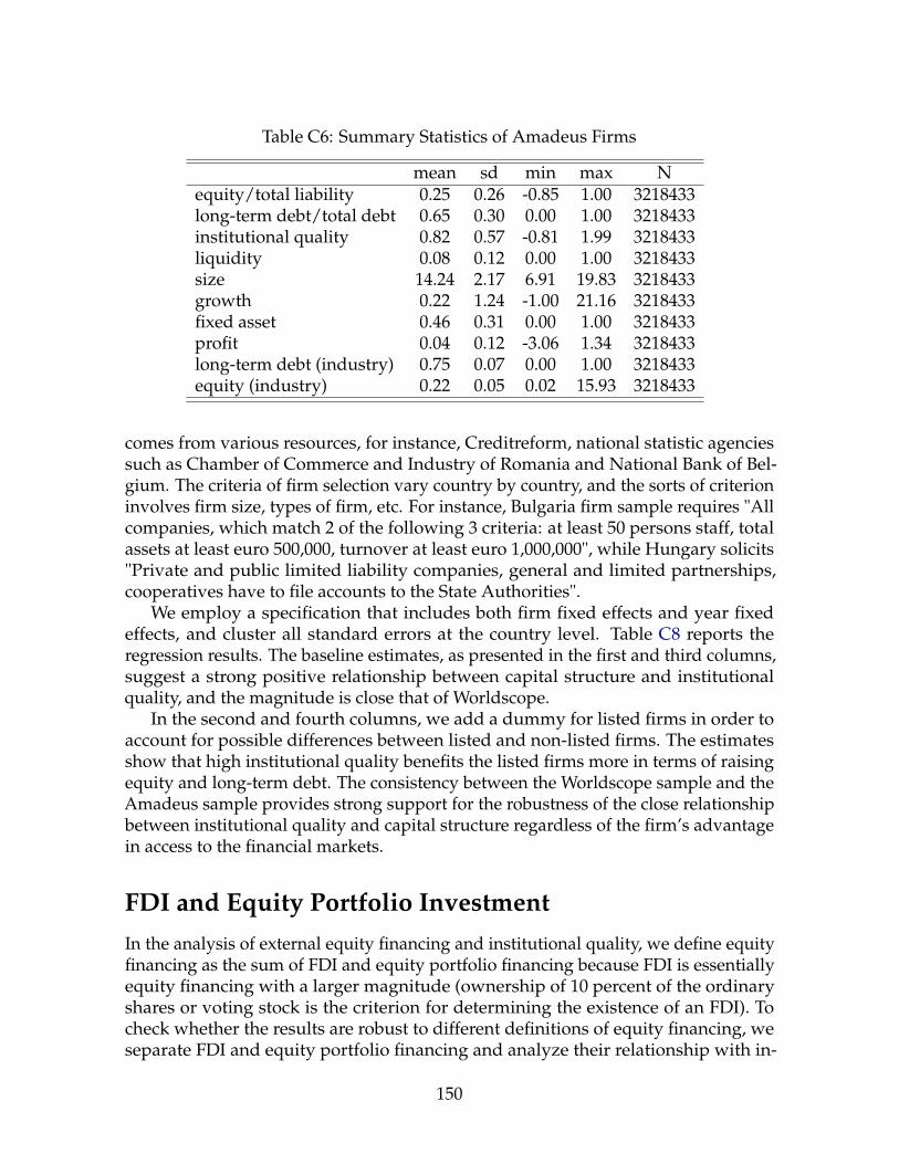
Table C6: Summary Statistics of Amadeus Firms

mean sd min max Nequity/total liability 0.25 0.26 -0.85 1.00 3218433long-term debt/total debt 0.65 0.30 0.00 1.00 3218433institutional quality 0.82 0.57 -0.81 1.99 3218433liquidity 0.08 0.12 0.00 1.00 3218433size 14.24 2.17 6.91 19.83 3218433growth 0.22 1.24 -1.00 21.16 3218433fixed asset 0.46 0.31 0.00 1.00 3218433profit 0.04 0.12 -3.06 1.34 3218433long-term debt (industry) 0.75 0.07 0.00 1.00 3218433equity (industry) 0.22 0.05 0.02 15.93 3218433

comes from various resources, for instance, Creditreform, national statistic agenciessuch as Chamber of Commerce and Industry of Romania and National Bank of Bel-gium. The criteria of firm selection vary country by country, and the sorts of criterioninvolves firm size, types of firm, etc. For instance, Bulgaria firm sample requires "Allcompanies, which match 2 of the following 3 criteria: at least 50 persons staff, totalassets at least euro 500,000, turnover at least euro 1,000,000", while Hungary solicits"Private and public limited liability companies, general and limited partnerships,cooperatives have to file accounts to the State Authorities".

We employ a specification that includes both firm fixed effects and year fixedeffects, and cluster all standard errors at the country level. Table C8 reports theregression results. The baseline estimates, as presented in the first and third columns,suggest a strong positive relationship between capital structure and institutionalquality, and the magnitude is close that of Worldscope.

In the second and fourth columns, we add a dummy for listed firms in order toaccount for possible differences between listed and non-listed firms. The estimatesshow that high institutional quality benefits the listed firms more in terms of raisingequity and long-term debt. The consistency between the Worldscope sample and theAmadeus sample provides strong support for the robustness of the close relationshipbetween institutional quality and capital structure regardless of the firm’s advantagein access to the financial markets.

FDI and Equity Portfolio InvestmentIn the analysis of external equity financing and institutional quality, we define equityfinancing as the sum of FDI and equity portfolio financing because FDI is essentiallyequity financing with a larger magnitude (ownership of 10 percent of the ordinaryshares or voting stock is the criterion for determining the existence of an FDI). Tocheck whether the results are robust to different definitions of equity financing, weseparate FDI and equity portfolio financing and analyze their relationship with in-

150

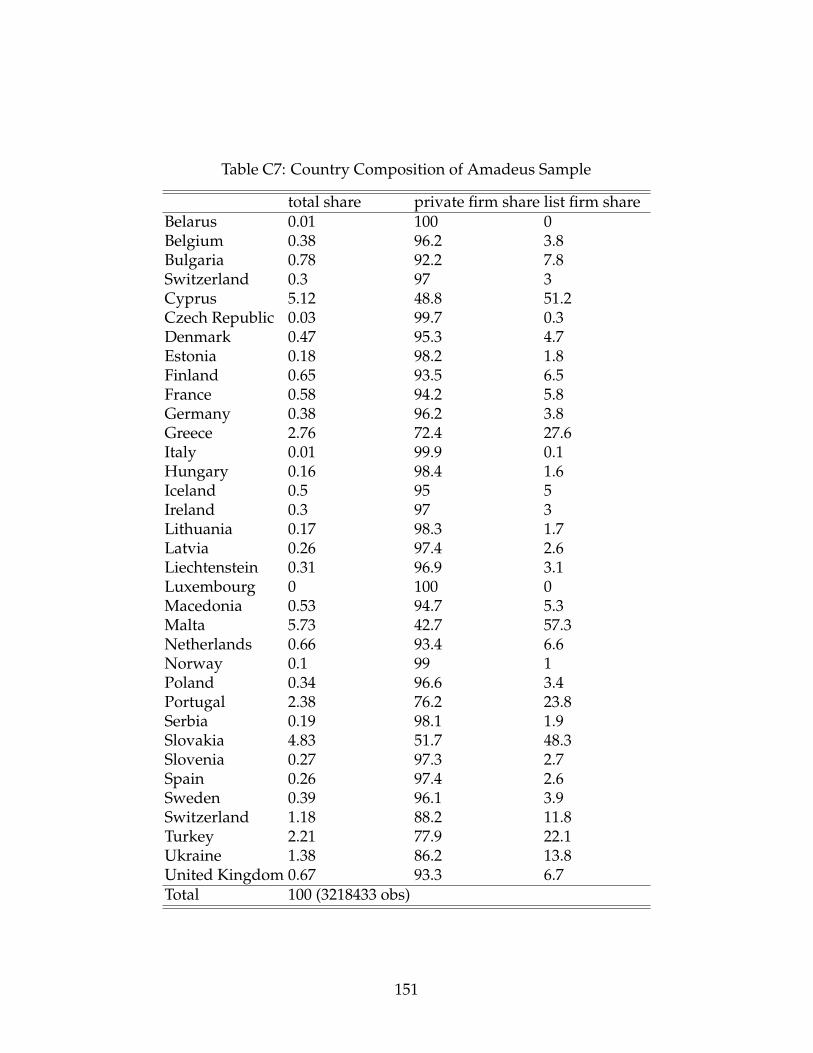
Table C7: Country Composition of Amadeus Sample

total share private firm share list firm shareBelarus 0.01 100 0Belgium 0.38 96.2 3.8Bulgaria 0.78 92.2 7.8Switzerland 0.3 97 3Cyprus 5.12 48.8 51.2Czech Republic 0.03 99.7 0.3Denmark 0.47 95.3 4.7Estonia 0.18 98.2 1.8Finland 0.65 93.5 6.5France 0.58 94.2 5.8Germany 0.38 96.2 3.8Greece 2.76 72.4 27.6Italy 0.01 99.9 0.1Hungary 0.16 98.4 1.6Iceland 0.5 95 5Ireland 0.3 97 3Lithuania 0.17 98.3 1.7Latvia 0.26 97.4 2.6Liechtenstein 0.31 96.9 3.1Luxembourg 0 100 0Macedonia 0.53 94.7 5.3Malta 5.73 42.7 57.3Netherlands 0.66 93.4 6.6Norway 0.1 99 1Poland 0.34 96.6 3.4Portugal 2.38 76.2 23.8Serbia 0.19 98.1 1.9Slovakia 4.83 51.7 48.3Slovenia 0.27 97.3 2.7Spain 0.26 97.4 2.6Sweden 0.39 96.1 3.9Switzerland 1.18 88.2 11.8Turkey 2.21 77.9 22.1Ukraine 1.38 86.2 13.8United Kingdom 0.67 93.3 6.7Total 100 (3218433 obs)

151

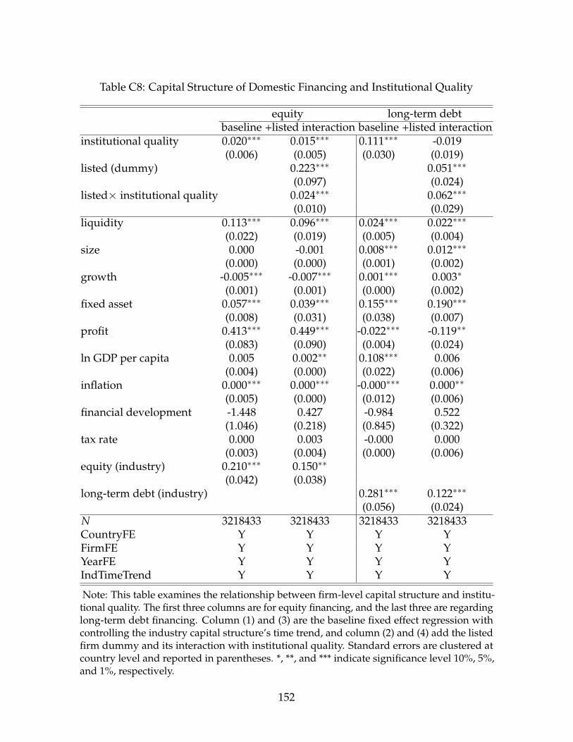
Table C8: Capital Structure of Domestic Financing and Institutional Quality

equity long-term debtbaseline +listed interaction baseline +listed interaction

institutional quality 0.020∗∗∗ 0.015∗∗∗ 0.111∗∗∗ -0.019(0.006) (0.005) (0.030) (0.019)

listed (dummy) 0.223∗∗∗ 0.051∗∗∗

(0.097) (0.024)listed× institutional quality 0.024∗∗∗ 0.062∗∗∗

(0.010) (0.029)liquidity 0.113∗∗∗ 0.096∗∗∗ 0.024∗∗∗ 0.022∗∗∗

(0.022) (0.019) (0.005) (0.004)size 0.000 -0.001 0.008∗∗∗ 0.012∗∗∗

(0.000) (0.000) (0.001) (0.002)growth -0.005∗∗∗ -0.007∗∗∗ 0.001∗∗∗ 0.003∗

(0.001) (0.001) (0.000) (0.002)fixed asset 0.057∗∗∗ 0.039∗∗∗ 0.155∗∗∗ 0.190∗∗∗

(0.008) (0.031) (0.038) (0.007)profit 0.413∗∗∗ 0.449∗∗∗ -0.022∗∗∗ -0.119∗∗

(0.083) (0.090) (0.004) (0.024)ln GDP per capita 0.005 0.002∗∗ 0.108∗∗∗ 0.006

(0.004) (0.000) (0.022) (0.006)inflation 0.000∗∗∗ 0.000∗∗∗ -0.000∗∗∗ 0.000∗∗

(0.005) (0.000) (0.012) (0.006)financial development -1.448 0.427 -0.984 0.522

(1.046) (0.218) (0.845) (0.322)tax rate 0.000 0.003 -0.000 0.000

(0.003) (0.004) (0.000) (0.006)equity (industry) 0.210∗∗∗ 0.150∗∗

(0.042) (0.038)long-term debt (industry) 0.281∗∗∗ 0.122∗∗∗

(0.056) (0.024)N 3218433 3218433 3218433 3218433CountryFE Y Y Y YFirmFE Y Y Y YYearFE Y Y Y YIndTimeTrend Y Y Y Y

Note: This table examines the relationship between firm-level capital structure and institu-tional quality. The first three columns are for equity financing, and the last three are regardinglong-term debt financing. Column (1) and (3) are the baseline fixed effect regression withcontrolling the industry capital structure’s time trend, and column (2) and (4) add the listedfirm dummy and its interaction with institutional quality. Standard errors are clustered atcountry level and reported in parentheses. *, **, and *** indicate significance level 10%, 5%,and 1%, respectively.

152

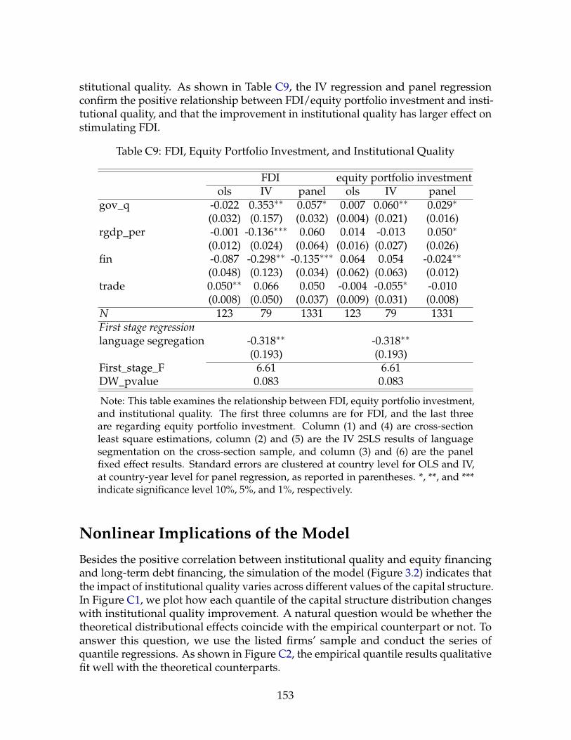
stitutional quality. As shown in Table C9, the IV regression and panel regressionconfirm the positive relationship between FDI/equity portfolio investment and insti-tutional quality, and that the improvement in institutional quality has larger effect onstimulating FDI.

Table C9: FDI, Equity Portfolio Investment, and Institutional Quality

FDI equity portfolio investmentols IV panel ols IV panel

gov_q -0.022 0.353∗∗ 0.057∗ 0.007 0.060∗∗ 0.029∗

(0.032) (0.157) (0.032) (0.004) (0.021) (0.016)rgdp_per -0.001 -0.136∗∗∗ 0.060 0.014 -0.013 0.050∗

(0.012) (0.024) (0.064) (0.016) (0.027) (0.026)fin -0.087 -0.298∗∗ -0.135∗∗∗ 0.064 0.054 -0.024∗∗

(0.048) (0.123) (0.034) (0.062) (0.063) (0.012)trade 0.050∗∗ 0.066 0.050 -0.004 -0.055∗ -0.010


(0.193) (0.193)First_stage_F 6.61 6.61DW_pvalue 0.083 0.083

Note: This table examines the relationship between FDI, equity portfolio investment,and institutional quality. The first three columns are for FDI, and the last threeare regarding equity portfolio investment. Column (1) and (4) are cross-sectionleast square estimations, column (2) and (5) are the IV 2SLS results of languagesegmentation on the cross-section sample, and column (3) and (6) are the panelfixed effect results. Standard errors are clustered at country level for OLS and IV,at country-year level for panel regression, as reported in parentheses. *, **, and ***indicate significance level 10%, 5%, and 1%, respectively.

Nonlinear Implications of the ModelBesides the positive correlation between institutional quality and equity financingand long-term debt financing, the simulation of the model (Figure 3.2) indicates thatthe impact of institutional quality varies across different values of the capital structure.In Figure C1, we plot how each quantile of the capital structure distribution changeswith institutional quality improvement. A natural question would be whether thetheoretical distributional effects coincide with the empirical counterpart or not. Toanswer this question, we use the listed firms’ sample and conduct the series ofquantile regressions. As shown in Figure C2, the empirical quantile results qualitativefit well with the theoretical counterparts.

153

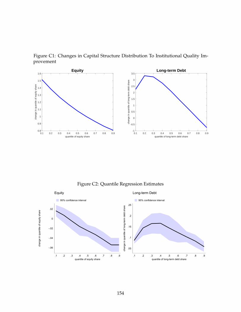
Figure C1: Changes in Capital Structure Distribution To Institutional Quality Im-provement

0.1 0.2 0.3 0.4 0.5 0.6 0.7 0.8 0.9quantile of equity share

0.8

0.9

1

1.1

1.2

1.3

1.4

1.5

1.6

chan

ge in

qua

ntile

of e

quity

sha

re

Equity

0.1 0.2 0.3 0.4 0.5 0.6 0.7 0.8 0.9quantile of long-term debt share

-1

-0.5

0

0.5

1

1.5

2

2.5

3

3.5

chan

ge in

qua

ntile

of l

ong-

term

deb

t sha

re

Long-term Debt

Figure C2: Quantile Regression Estimates

-.06

-.04

-.02

0

.02

chan

ge in

qua

ntile

of e

quity

sha

re

.1 .2 .3 .4 .5 .6 .7 .8 .9quantile of equity share

95% confidence interval

Equity

.05

.1

.15

.2

.25

chan

ge in

qua

ntile

of l

ong-

term

deb

t sha

re

.1 .2 .3 .4 .5 .6 .7 .8 .9quantile of long-term debt share

95% confidence interval

Long-term Debt

154

Essays in International Economics - Academic Commons

Documents

Transcript of Essays in International Economics - Academic Commons