ESRI ArcMap 10.1 Manualgeo-tiff.com/outlines/arcmapmanual.pdf · Check on ‘Automatically Delete...

ESRI ArcMap 10.1 Manual MGEO 2014

0

ESRI ArcMap 10.1 Manual

For Hydrography & Survey Use.

MGEO 2014

Tiffany Schnare www.Geo-Tiff.com

MGEO 2014 Brian Pyke

May 30, 2013


1

Foreward

The following document was produced with the Marine Geomatics instructor, Brian Pyke in mind. Students from the 2014 Marine Geomatics Class were observed throughout the year to gain an understanding of what would benefit hydrographers to understand in an ArcMap environment. These students use GPS equipment to collect hydrographic survey data but they typically do no possess the experience needed to produce useful maps/charts; this manual will give guidance and aid when creating a final product and analyzing data.


2

Table of Contents 1 Important to Remember! ........................................................................................................................ 1

1.1 Files & Folders ..................................................................................................................................... 1

1.2 Store Relative Paths .......................................................................................................................... 1

1.3 Storage Space .................................................................................................................................. 1

2 Creating Blank Shapefiles ....................................................................................................................... 2

2.1 With a tool: ......................................................................................................................................... 2

2.2 With an existing Shapefile: .............................................................................................................. 3

3 Adding Points ............................................................................................................................................. 4

3.1 Using Excel: ........................................................................................................................................ 4

4 Creating a Study Area ............................................................................................................................. 5

4.1 Using the Drawing Toolbar: ............................................................................................................. 5

5 .TXT to .SHP .................................................................................................................................................. 6

6 Annotating Sounding Features .............................................................................................................. 7

7 Generalizing/Editing Soundings ............................................................................................................. 8

8 Batch Processing ....................................................................................................................................... 9

8.1 Clipping .............................................................................................................................................. 9

9 Creating Graticules/Grids ..................................................................................................................... 10

9.1 Graticule........................................................................................................................................... 10

9.2 Measured Grid ................................................................................................................................ 11

9.3 Reference Grid ............................................................................................................................... 12

10 Setting-up a Data Frame .................................................................................................................. 13

11 Importing a GeoTiff ............................................................................................................................. 14

12 Geo-Rectifying .................................................................................................................................... 15

13 Creating a Digital Elevation Model (DEM) ..................................................................................... 17

14 Calculating Flow Direction and Accumulation ............................................................................ 18

15 Ocean Bottom Shading using Soundings ...................................................................................... 19

16 Digitize ................................................................................................................................................... 20

16.1 From Side Scan Mosaics ................................................................................................................ 20

17 Temporarily Clip Data ........................................................................................................................ 21

18 Creating Contours from Sounding Points ....................................................................................... 22

19 Cleaning Contours ............................................................................................................................. 23

20 Backing-up to a CD ........................................................................................................................... 24


1

1 Important to Remember! The following is a list of tips & tricks that I find helpful when working in an ArcMap environment.

1.1 Files & Folders It is good practice to NEVER use spaces or special characters in file or folder

names; especially when using ESRI software; many processes will not run correctly with these and it will be a pain to change file/folder names and source paths in the middle of a project. Instead of using spaces use underscores (_); this is the only special character that should be used. All others might also not be supported.

Instead of burying MXDs and Data under folder after folder create a new folder at the root of your drive for EACH PROJECT. Keep the path names short and simple. This will prove to be helpful when you have to pass in projects or burn them to disks for clients.

1.2 Store Relative Paths As soon as you open ArcMap, even before you save the project, set the

document to store relative path names. To do so:

1. File > Map Document Properties > Check on ‘Store relative pathnames to data sources’

2. Save your document This will ensure the data will still be found if you move the document.

1.3 Storage Space Estimate the amount of storage you will need and double it; this is the amount of

storage space you should have on your default drive. Make sure to have a completely separate location (i.e. an external drive) that

also has the same amount of free space; back up ALL of your project files to this drive whenever you have completed any major changes or analyses.


2

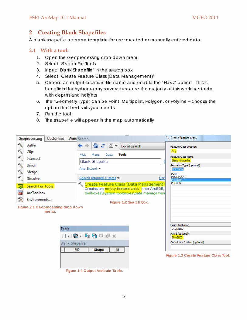
2 Creating Blank Shapefiles A blank shapefile acts as a template for user created or manually entered data.

2.1 With a tool: 1. Open the Geoprocessing drop down menu 2. Select ‘Search For Tools’ 3. Input: ‘Blank Shapefile’ in the search box 4. Select ‘Create Feature Class (Data Management)’ 5. Choose an output location, file name and enable the ‘Has Z’ option – this is

beneficial for hydrography surveys because the majority of this work has to do with depths and heights

6. The ‘Geometry Type’ can be Point, Multipoint, Polygon, or Polyline – choose the option that best suits your needs

7. Run the tool 8. The shapefile will appear in the map automatically

Figure 1.2 Search Box. Figure 2.1 Geoprocessing drop down

menu.

Figure 1.3 Create Feature Class Tool.

Figure 1.4 Output Attribute Table.


3

2.2 With an existing Shapefile: Note: This method is particularly good if you have an existing Shapefile with the attribute fields that you want in a new Shapefile.

1. Using ‘Add Data’ import the existing Shapefile 2. Right click on Shapefile 3. ‘Select Data’ > ‘Export Data’ 4. Rename the Shapefile and select output location 5. Add layer to map 6. Right click on Shapefile 7. Select ‘Edit Features’ > ‘Start Editing’ 8. Open Attribute Table 9. Select all records

10. Delete 11. Save Edits 12. Exit Editor

Figure 1.5 Export Data with a new name.

Figure 1.6 Start editing data.

Figure 1.7 Open Attribute Table & Select all records.

Figure 1.8 Save edits and stop editing.


4

3 Adding Points Point data can be from a multitude of sources, such as from; total stations, RTK, SBES, MBES, government websites, etc. The following will outline how to bring the data into ArcMap for analyses and presentation

3.1 Using Excel: 1. Open a blank Excel file 2. Create the following headings: Id, Northing, Easting, Zvalue 3. Input the coordinates and height values in the proper fields 4. Start the Id field at 0 and continue numbering each record sequentially 5. Save the Excel file

6. Import the .xlsx file using ‘Add Data’ 7. Right click on the file in the Table Of Contents 8. Select ‘Display XY Data 9. Select Easting for the X Field, Northing for the Y Field and Zvalue for the Z Field. 10. Choose the associated coordinate system 11. Select ‘OK’ 12. Right click on file 13. Select ‘Data’ > ‘Export Data’ 14. Add layer to map and delete the

previous two file.

Figure 3.1 Excel file with field headings.

Figure 3.2 Display XY Data.

Figure 3.3 Display XY Data with proper inputs.


5

4 Creating a Study Area A study area outlines the area that the user will be analyzing. Having a study area allows the user to use tools (i.e. a buffer) on just a specific area; this will save time as the tools do not need to be run on superfluous data.

4.1 Using the Drawing Toolbar: 1. On the Draw toolbar select the appropriate draw method – Polygon works well

for most applications 2. Draw the boundary for the study area 3. Select the finished drawing 4. Open the drawing drop down menu on the Draw toolbar 5. Select ‘Convert Graphics to Features…’ 6. Choose an output location and Shapefile name 7. Check on ‘Automatically Delete Graphics after conversion’ 8. Add layer to map

Figure 4.1 Draw toolbar with draw methods drop down menu.

Figure 4.4 Finished drawing shown in yellow.

Figure 4.2 Draw toolbar with Drawing pull down menu.

Figure 4.3 Convert Graphics to Features.


6

5 .TXT to .SHP The following process will take coordinates from a text file and turn them into a Shapefile which can be displayed and analyzed.

Note: This will be particularly useful when large files of data with Northings/Eastings or Latitudes/Longitudes are obtained and are needed to be displayed or analyzed.

1. Start by opening the file in a text editor such as Microsoft Excel 2. Ensure the data is correctly formatted:

a. Columns with coordinates should all be set to number and the same decimal place

b. All columns must have a column heading (no spaces or special characters, keep it as short as possible)

c. An ‘ObjectID’ column must be added; this will start at zero and number the following rows sequentially

3. Add the .txt file using ‘Add Data’ 4. Right click on the file in the ‘Table of Contents’ 5. Select ‘Display XY Data’ 6. Select the proper fields as Northing, Easting, and Depth values 7. Select the proper coordinate system > OK

The data is now displayed as a Shapefile is but it is still in text file format 8. Right click on the newly added layer in the ‘Table of Contents’ (This should be

the layer named: ‘filename.txt Events’ 9. ‘Data’ > ‘Export Data…’ 10. Set the inputs to the following:

a. Export: All Features b. Use the same coordinate system as: the data frame c. Click the folder button: rename the Output Feature Class and point

towards suitable folder; Change the ‘Save as type…’ is set to Shapefile unless saving to a Geodatabase

11. Add to map 12. Delete the previous two layers


7

6 Annotating Sounding Features The following process will take the soundings obtained from a MBES, or SBES then display them as values on a chart.

1. Bring in Sounding features using ‘Add Data’ 2. Open the ‘Layer Properties’ window 3. Go to the ‘Symbology’ tab 4. Set the points to have no color or outline 5. Go to the ‘Labels’ tab 6. Check on ‘Label features in this layer’ box 7. Method: ‘Label all the features the same way’ 8. A VB Script will need to be used to achieve a sounding with decimal values in

italics: a. Open the ‘Expression’ window b. Check on ‘Advanced’ c. Copy and paste the script from Appendix A to the input box d. ‘Verify’ the script

9. The font type and size will depend on the scale and use of the chart 10. Apply the changes and refresh the Data View

Figure 6.1 Soundings Symbolization

Figure 6.3 Label Tab in Layer Properties

Figure 6.2 Label Expression window with advanced script


8

7 Generalizing/Editing Soundings Sometimes hundreds or more soundings can be taken in one location meaning there will be many overlapping points when the data is displayed in Arcmap; the following will thin out the data to make it easier to read.

Note: Care should be taken when editing Sounding information so that they are not moved, replaced, or changed in any major way. This system is only if the soundings are too dense in a particular area for the chart to be legible at its set scale.

1. Once the Soundings have been labeled to an acceptable standard (see section 6 – Annotating Sounding Features) they need to be converted to an annotation layer for ease of editing, once this is done the font, color, size, etc. cannot be changed;

a. Open ‘Data Frame Properties’ – ‘General’ tab b. Set the ‘Label Engine’ to ‘Maplex Label Engine’ c. Right click on Sounding feature Shapefile that is associated with the labels d. ‘Convert Labels to Annotation’ e. If all data is stored in a Geodatabase then choose to ‘Store Annotation’ –

‘In a Database’, otherwise choose ‘In the Map’ f. Convert

2. An annotation layer will be added to the map > Right click 3. ‘Edit Features’ > ‘Start Editing’

4. Using the tool select the sounding(s) you wish to delete

5. Right click with the sounding(s) still selected > Delete In the beginning if you are unsure of how many soundings to delete follow this rule of thumb: Select a sounding you believe is in a decent location and would like to keep, and then delete the nearest top, bottom, left, and right soundings.

Figure 7.3 Soundings to be deleted highlighted in blue

Figure 7.1 Where to find ‘Convert Labels to Annotation’ Figure 7.2 'Convert Labels to Annotation' window with

inputs


9

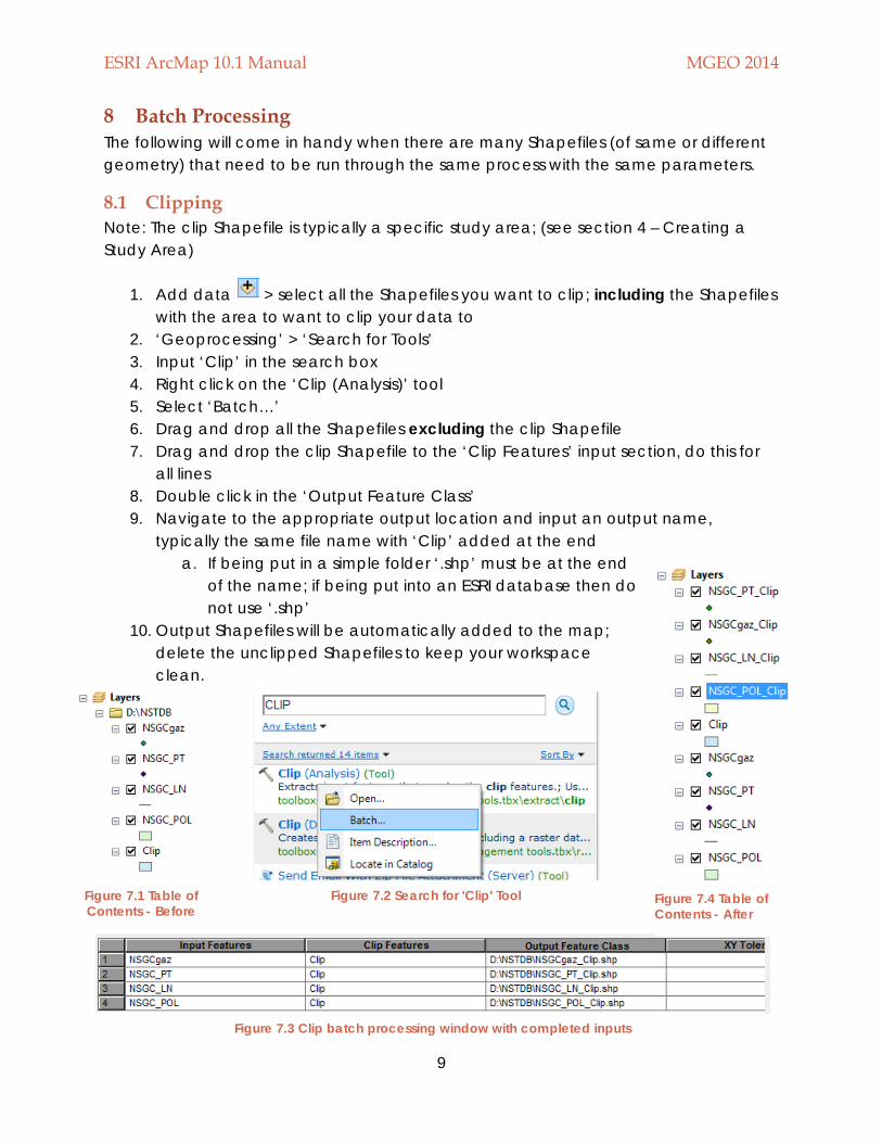
8 Batch Processing The following will come in handy when there are many Shapefiles (of same or different geometry) that need to be run through the same process with the same parameters.

8.1 Clipping Note: The clip Shapefile is typically a specific study area; (see section 4 – Creating a Study Area)

1. Add data > select all the Shapefiles you want to clip; including the Shapefiles with the area to want to clip your data to

2. ‘Geoprocessing’ > ‘Search for Tools’ 3. Input ‘Clip’ in the search box 4. Right click on the ‘Clip (Analysis)’ tool 5. Select ‘Batch…’ 6. Drag and drop all the Shapefiles excluding the clip Shapefile 7. Drag and drop the clip Shapefile to the ‘Clip Features’ input section, do this for

all lines 8. Double click in the ‘Output Feature Class’ 9. Navigate to the appropriate output location and input an output name,

typically the same file name with ‘Clip’ added at the end a. If being put in a simple folder ‘.shp’ must be at the end

of the name; if being put into an ESRI database then do not use ‘.shp’

10. Output Shapefiles will be automatically added to the map; delete the unclipped Shapefiles to keep your workspace clean.

Figure 7.1 Table of Contents - Before

Figure 7.2 Search for 'Clip' Tool Figure 7.4 Table of Contents - After

Figure 7.3 Clip batch processing window with completed inputs


10

9 Creating Graticules/Grids Graticules and Grids are seen surrounding maps; the user can extract coordinates of interest from them.

9.1 Graticule Note: This method is useful if the users will require or utilizing Latitude and Longitude coordinates.

1. Open Data Frame Properties: Right Click on ‘Layers’ > ‘Properties’ 2. Open the ‘Grid’ Tab 3. Select ‘New Grid’ 4. Select ‘Graticule’ > Next 5. The intervals will depend on the scale and purpose of the map:

a. If the map is large scale or a simple keymap then the intervals can be larger (i.e. degrees)

b. If the map is small scale then intervals will need to be smaller as well so they will be displayed (i.e. minutes or seconds)

> Next 6. Uncheck ‘Minor division ticks’ 7. The test style should be the same as a text style previously used on the map

(maps should only have upwards of three text styles) > Next 8. The ‘Graticule Border’ is typically has three lines of gradual increasing width at a

width of between 1 and 2 > Finish 9. The Grid creation window will close and ‘Graticule’ will be added to the list to

the left 10. Select the newly created graticule > ‘Properties’ 11. On the ‘Labels’ tab under ‘Label Orientation > Vertical Labels’ check on Left

and Right

Figure 9.1 Open Data Frame Properties

Figure 9.2 Add a New Grid

Figure 9.3 The most common border used during Grid

creation

Figure 9.4 Rotate the Left and Right labels


11

9.2 Measured Grid Note: This method is useful if the users will require or utilizing Easting and Northing coordinates.

1. Open Data Frame Properties: Right Click on ‘Layers’ > ‘Properties’ 2. Under the ‘General tab’ change ‘Units > ‘Map’ from unknown to the units that

the final map will be utilizing 3. Open the ‘Grid’ Tab 4. Select ‘New Grid’ 5. Select ‘Measured Grid’ > Next 6. ‘Appearance’ should be set to display ‘ Grid and labels’ 7. The intervals will depend on the scale and purpose of the map:

a. If the map is large scale or a simple keymap then the intervals can be larger (i.e. 100<)

b. If the map is small scale then intervals will need to be smaller as well so they will be displayed (i.e. 100>)

> Next 8. Uncheck ‘Minor division ticks’ 9. Text style should be similar to that used on the map and bold 10. The border for a measure grid is typically a simple black line with a width

between 1 and 3 > Finish 11. The Grid creation window will close and ‘Measured Grid’ will be added to the list

to the left 12. Select the newly created measure grid > ‘Properties’ 13. On the ‘Labels’ tab under ‘Label Orientation > Vertical Labels’ check on Left

and Right

Figure 9.7 Change Map Units

Figure 9.5 Appearance should be set to Grid and

labels Figure 9.6 Typically a

simple border is used for this method


12

9.3 Reference Grid Note: This method is useful if the final map will not utilize coordinates is a specific coordinate system; rather the area will be divided into a specific number of columns and rows which will create numerous boxed areas with a unique row and column value. Example: the National Topographic System Index Map

1. Open Data Frame Properties: Right Click on ‘Layers’ > ‘Properties’ 2. Open the ‘Grid’ Tab 3. Select ‘New Grid’ 4. Select ‘Reference Grid’ > Next 5. ‘Appearance’ should be set to display ‘ Grid and index tabs’ 6. The intervals will depend on the shape of the area and how big/small each

section needs to be: a. If the study area is longer than it is wide the number of columns will

increase; If the study area is wider than it is long the number of rows will increase

> Next 7. Tab style is a matter of preference but the color should be one that is similar to

those used in the map thus far; pink is default and I suggest that it not be used 8. Text style should be similar to that used on the map and ALL CAPS 9. Typically there is no added border to an Index Grid > Finish 10. The Grid creation window will close and ‘Index Grid’ will be added to the list to

the left

Figure 9.9 Intervals will depend on shape and size

Figure 9.8 The Button Type is only a matter of preference there is none more common

then another


13

10 Setting-up a Data Frame The data frame is the settings for the map; such as how the data will be displayed (i.e. coordinate system and scale).

Note: Many of the values when setting-up a data frame depend on the data and final scale of the map; therefore this demonstration will assume a small scale map in the Nova Scotia area.

1. Open Data Frame Properties: Right Click on ‘Layers’ > ‘Properties’ 2. Under the ‘General’ tab set:

a. ‘Units > ‘Map’ and ‘Display’ to Meters b. ‘Reference Scale’ to 1:10,000

3. Under the ‘Data Frame’ tab set: a. ‘Extent’ to ‘Fixed Scale > Use Current Scale’ b. If a study area Shapefile is being used then set ‘Extent Used by Full Extent

Command’ to ‘Other’> open ‘Specify Extent’> select ‘Outline of Features’ > select the study area Shapefile (This will make it so the ‘Full Extent’ button will zoom to the extent of the study area)

4. Under the ‘Coordinate System’ tab navigate or search for NAD 1983 UTM Zone 20N and select

5. Create a Grid (see section 9 - Creating Graticules/Grids) 6. Under the ‘Frame’ tab

a. Input an X and Y gap of 30 b. Select a double line, graded border – black

Figure 10.1 General Tab

Figure 10.2 Data Frame Tab

Figure 10.3 Specific Extent Window

Figure 10.1 Frame Tab


14

11 Importing a GeoTiff A GeoTiff is an image (i.e. air photo or map) with a location on the ground. Therefore it can be displayed in the correct location behind data to provide additional information.

Note: If a raster file (.tiff or .tif) comes with a world file (.tfw) that is EXACTLY the same name (i.e. Image123.tiff and Image123.tfw) then it is a GeoTiff.

1. Open Data Frame Properties: Right Click on ‘Layers’ > ‘Properties’ 2. Under the ‘Coordinate System’ tab set to the projection associated with the

GeoTiff > Apply & Okay 3. Open ‘Add Data’ 4. Navigate to the folder that contains the GeoTiff 5. Click on the file ONLY ONCE > Add (Clicking more than once will only bring in

specific bands of color and the image will not be displayed correctly) 6. Right click on the image in the table of contents > ‘Properties’ 7. Under the ‘Symbology’ tab set the ‘Stretch Type’ to None

Figure 11.1 Make sure there is an associated .tfw file

Figure 11.2 Add Raster file

Figure 11.3 Result of Double-Clicking the Raster file

Figure 11.4 Symbology of the raster; stretch should be None


15

12 Geo-Rectifying This process will take an image (i.e. air photo or map) and give it a place on the earth. Meaning the image can be brought in behind data for additional information.

Note: For this process to work two files are necessary: at least one file to act as a reference file (typically a Shapefile, such as a roads layer) with an attached coordinate system and one file to be rectified (typically a raster image) without a coordinate system, these files must be from the same location on earth. See next page for images.

1. Set up the Coordinate system in the Data Frame Properties 2. Add the reference file 3. Add the raster file 4. Open the properties window for the raster file > Under the ‘Display’ tab set the

transparency to 50% 5. ‘Customize’ pull down menu > ’Toolbars’ > Select ‘Georeferencing’ if it does not

have a checkmark beside it, if it does do not click it 6. Right-Click on the reference layer > ‘Zoom to Layer’ 7. On the ‘Georeferencing’ toolbar:

a. Make sure the file name shown on the ‘Georeferencing’ toolbar matches that of the file you want to rectify

b. Open the ‘Georeferencing’ pull down menu > ‘Fit to Display’

8. Open the pull down menu; use these tools to roughly place the raster in the correct location using the reference layer for guidance

9. Select the (add control points) tool > Find a location on the raster that is also easy to find on the reference layer

a. First select the location on the raster b. Then select the same location on the reference layer

The map will automatically move to attempt to fit the raster file to the specified location

10. More control points will need to be added evenly throughout the area for proper georeferencing

11. Once the raster fits well enough for the intended use open the ‘Georeferencing’ pull down menu and select ‘Recify…’

a. Select the folder icon and navigate to the proper location; click only once on the folder where you want to file to be placed > Add

b. Input a file name, ideally the same name as the file previously had with ‘rect’ added to the end of it

c. ‘Compression Type’ as NONE d. Save

12. Delete the unrectified file from the table of contents 13. Add the rectified file to the map


16

Figure 13.1 Add the Georeferencing toolbar

Figure 13.2 Fit the Raster to the display

Figure 12.1 Roughly fit the raster to the

proper location

Figure 13.4 Add Control Points

Figure 12.2 Export the file to permanently rectify the image


17

13 Creating a Digital Elevation Model (DEM) A Digital Elevation Model takes elevation data from contours and creates a 3D representation of the terrain.

Note: The ‘Topo to raster’ tool used in this exercise can input many Shapefiles at once to enhance the quality of the output, ex. Contours and streams would output a DEM of a higher caliber then Contours only would. On the other hand this tool can also be run with either contours or spot elevations and nothing extra.

1. Set Coordinate System in ‘Data Frame Properties’

2. Add contours 3. Right-Click on contours layer > ‘Data’ > ‘Export Data…’

a. ‘Use the same coordinate system as:’ - ‘the data frame’ 4. ‘Geoprocessing’ > ‘Search For Tools’ > ‘Topo to Raster (3D Analyst)’

a. Input contour Layer > set field to ‘Elevation’ > Type to ‘Contour’ b. For the initial run-through keep the default ‘Output cell size’ c. Set an appropriate output location and file name

5. At first this will not look the same as the DEM typically seen; to change this Right-Click on the layer > Symbology > ‘Classified’ > Choose a white to black color ramp

Figure 13.2 Initial Contour Layer Figure 13.1 Topo to Raster Output DEM

Figure 13.3 Final DEM


18

14 Calculating Flow Direction and Accumulation This process will determine the direction water will flow and accumulate in a certain location based on the Digital Elevation Model (DEM) of the terrain.

Note: A DEM raster network is required for this exercise; DEMs can be acquired for any location in Canada at www.GeoBase.ca, DEMs can also be manually created for other locations. This example will use a 1:50 000 GeoBase DEM raster from the North Vancouver area (ID 092G06).

1. Set the Correct coordinate system; if this step is done incorrectly the process will not work

2. Add DEMs to map (If using GeoBase data they come in two files – East and West; therefore the following steps will need to be performed twice)

a. When asked to ‘Create Pyramids’ select YES 3. Right-Click on the raster layer > ‘Data’ > ‘Export Data’

a. Change the output file type to ‘IMAGINE Image’ b. For ‘Spatial Reference’ select ‘Data Frame (Current)’ c. Choose an Appropriate output location

This will permanently associate the coordinate system set in step 1 to the rasters) 4. Delete the .dem rasters 5. ‘Geoprocessing’ > ‘Search for Tools’ > Search for ‘Fill (Spatial Analyst)’

a. Input: .img raster b. Output: DEM_Fill.tif (Make sure to have ‘.tif’ at the end of the name)

6. ‘Geoprocessing’ > ‘Search for Tools’ > Search for ‘Fill (Spatial Analyst)’ a. Input: DEM_Fil.tif b. Output: FlowDir

7. ‘Geoprocessing’ > ‘Search for Tools’ > Search for ‘Flow Accumulation (Spatial Analyst)’

a. Input: DEM_Fil.tif b. Output: FlowAcc.tif

Figure 15.2 Areas of high water accumulaion

Figure 15.1 Flow Direction

http://www.geobase.ca/


19

15 Ocean Bottom Shading using Soundings Other then the Soundings the user can perceive the rate of depth change in the study area by shading. On charts the white area is the deepest and the darkest area is the shallowest.

1. Add Soundings 2. Open ‘ET GeoWizards’ > ‘Surface’ tab 3. Select ‘Build PolygonZ TIN’ > GO

a. Input: Sounding Layer b. Output: Tin.shp

4. ‘Surface’ tab > select ‘Interpolate Contours’ > GO a. Input: Tin.shp b. Output: Contours.shp c. Contour Interval will depend on the size of the study area but for shading

purposes typically 1 Degree works best 5. Clean Contours (see section 19 – Cleaning Contours) 6. ‘Convert’ tab > ‘Polyline to Polygon’ > GO

a. Input: Contours.shp b. Output: ContourPoly.shp c. Force Closure: 1 Degree

7. Right-Click on ContoursPoly layer > ‘Properties…’ > ‘Symbolization’ tab a. Select ‘Categories’ > ‘Unique Values’

i. Value Field: ET_Height ii. Color Ramp: Choose either a default white to blue or create your

own (Charts use a reverse method for shading the water area; meaning the deepest areas are white and the shallow areas are blue.)

iii. ‘Add All Values’ iv. Uncheck ‘<all other values> v. Right-Click on any of the symbol icons > ‘Properties for All

Symbols…’ > set ‘outline color’ to ‘no color’ b. Apply & OK

Figure 16.1 Symbolization window Figure 16.2 Final shaded contours


20

16 Digitize Digitizing is when the user turns a GeoTiff into vector data by manually outline and assign attributes to significant features.

16.1 From Side Scan Mosaics Note: CARIS HIPS & SIPS can export side scan mosaics as a GeoTiff. This demonstration will assume we are digitizing sediment classes; digitizing different types of features may require a different type of Shapefile.

1. Add the Mosaic GeoTiff 2. Add/Create a blank POLY Shapefile (see section 2 – Creating Blank Shapefiles) 3. Right-Click on the Shapefile > ‘Edit Features’ > ‘Start Editing’ 4. Open the Editor pull down menu on the Editor toolbar > ‘Editing Windows’ >

‘Create Feautures’ 5. Select the Shapefile in the ‘Create Features’ window > in the ‘Construction Tools’

window select ‘Polygon’ or ‘Auto Complete Freehand’ 6. Start Digitizing features

Figure 17.1 Feature to be digitized

Figure 17.3 Digitized Polygon of the above feature Figure 17.2 Editor Toolbar


21

17 Temporarily Clip Data This requires at least two Shapefiles: a study area and a layer that falls within and extends beyond the study area. This process works well to clean-up the data view by not displaying extra data without actually deleting the data as the Clip tool will do. If the study area needs to be moved at a later time this method will accommodate that.

1. Add the Shapefiles 2. Open Data Frame Properties > ‘Data Frame’ tab 3. Change ‘Clip Options’ to ‘Clip to Shape’ 4. Open ‘Specific Shape…’ 5. Select ‘ Outline of Features’ > Choose the Study Area Shapefile 6. OK > Apply & OK

Figure 18.1 Before Clipping

Figure 18.2 After Clipping


22

18 Creating Contours from Sounding Points This process will turn sounding points into contour lines for further analyses.

1. Add the Soundings Shapefile to the map 2. ‘Customize’ > ‘Toolbars’ make sure that ‘ET GeoWizards’ is checked on 3. Open ‘ET Geowizards’ 4. Under ‘Surface’ select ‘Build PolygonZ TIN’ > ‘Go’ 5. Input layer is the Soundings, specify output location/name > Next 6. DEPTH is the elevation field > Finish 7. Under ‘Surface’ select ‘Interpolate Contours’ > ‘Go’ 8. Select the Tin Shapefile, specify output location/name > Next 9. Contour Interval will depend on scale and elevation change in the area, Base

Value remains set to zero 10. Remove the Tin and Soundings layers, you will be left with contours (These

contours will need to be cleaned. See section 19 – Cleaning Contours)

Figure 19.1 Sounding Points

Figure 19.2 Tin

Figure 19.3 Contours


23

19 Cleaning Contours Sometimes during contour creation if the area isn’t a perfect square or rectangle the tool will attempt to connect contours from opposite areas which do no actual connect; meaning the data is false and needs to be deleted.

1. Add the land Shapefile 2. Right-Click on the contours layer > ‘Edit Features’ > ‘Start Editing’ 3. For contour lines that are primarily on land

a. Select the line > Right-Click > Delete 4. For contour lines that are both on land and in the water

a. Select the line > Right-Click > ‘Edit Vertices’ b. Shift + left click on all green boxes (vertices) that are on land > Right-Click

> Delete 5. Once there are no contours that extend on land > Save Edits > Stop Editing

Figure 20.2 Incorrect contour on land highlighted in blue

Figure 20.1 Correct contour that extends slightly on land highlight in blue with vertices shown in green


24

20 Backing-up to a CD Backing-up the data allows the user the freedom and safety of knowing that the data can always be recovered as long as the CD is kept in a safe location.

Note: This method is only intended to be a back-up of a final project for an employer or a client not used as a safety net if your data is misplaced.

*This is where keeping the file paths short and all the data in the same location really comes in handy!

1. The file paths on the external must match exactly as they do in the default location:

a. Firstly; copy ALL of your folders with everything included to a completely separate location as a safety net

2. Assume the file path is ‘D:\GIS\Week08\FinalMap’ with the final MXD, shapefiles, geodatabase(s), and .PDF of the final plot in the ‘FinalMap’ folder

a. Create a ‘GIS’ folder on the CD, then within that create a ‘Week08’ Folder, and so on…

b. Copy AT LEAST the following files onto the CD under the ‘FinalMap’ folder: Final MXD, if a new MXD was created every week delete the

previous weeks MXDs Shapefiles, keep only the Shapefiles used on the final plot/if a

Geodatabase was used then copy only the Geodatabase and NOT the Shapefiles PDF of the final plot Anything else that is ABSOLUTLY needed, space on these externals

is minimal therefore unnecessary files take up too much room 3. Once all files are copied to the CD > ‘Burn to Disk’ as a DVD not as a USB 4. Insert the disk in a separate computer and open the MXD; if any of the layers

have red exclamation points next to them that implies the source file was not copied correctly to the CD.

a. Format the disk and try again.


25

APPENDIX A: Soundings Feature Script

Function FindLabel ( [DEPTH] )

IF ([DEPTH] < 0) then

Newlabdec = 0

Newlabdec = (Abs([DEPTH])-Int(Abs([DEPTH]))) * 10

FindLabel = "<ITA><UND>" & Abs(Fix([DEPTH])) & "</UND><SUB>" & Round (Newlabdec,1) & "</SUB></ITA>"

End If

Newlabdec = ([DEPTH]-Int([DEPTH])) * 10

IF ([DEPTH] > 0) and (Newlabdec = 0) then

FindLabel = "<ITA>" & Int([DEPTH]) & "</ITA>"

End If

IF ([DEPTH] > 0) and (Newlabdec <> 0) then

FindLabel = "<ITA>" & Int([DEPTH]) & "<SUB>" & Round (Newlabdec, 1) & "</SUB></ITA>"

End If

End Function

ESRI ArcMap 10.1 Manualgeo-tiff.com/outlines/arcmapmanual.pdf · Check on ‘Automatically Delete...

Documents

Transcript of ESRI ArcMap 10.1 Manualgeo-tiff.com/outlines/arcmapmanual.pdf · Check on ‘Automatically Delete...