ESA pointing error engineering handbook
72
Prepared by ESSB-HB-E-003 Working Group Reference ESSB-HB-E-003 Issue 1 Revision 0 Date of Issue 19 July 2011 Status Approved Document Type Handbook Distribution ESA UNCLASSIFIED – For Official Use ESA pointing error engineering handbook
Transcript of ESA pointing error engineering handbook

Prepared by ESSB-HB-E-003 Working Group
Reference ESSB-HB-E-003
Issue 1
Revision 0
Date of Issue 19 July 2011
Status Approved
Document Type Handbook
Distribution
ESA UNCLASSIFIED – For Official Use
ESA pointing error
engineering handbook

Page 2/72
ESSB-HB-E-003 Issue 1 Rev 0
Date 19 July 2011
ESA UNCLASSIFIED – For Official Use
Title ESA pointing error engineering handbook
Issue 1 Revision 0
Author ESSB-HB-E-003 Working Group Date 19 July 2011
Approved by ESB on behalf of ESSB Date 9 March 2011 (ESB#50)
Reason for change Ref/Issue Revision Date
First issue ESSB-HB-E-003
Issue 1
0 19 July 2011
Issue 1 Revision 0
Reason for change Date Pages Paragraph(s)

Page 3/72
ESSB-HB-E-003 Issue 1 Rev 0
Date 19 July 2011
ESA UNCLASSIFIED – For Official Use
Table of contents
Introduction ........................................................................................................................ 8
1 Scope ............................................................................................................................... 9
2 References .................................................................................................................... 10
2.1 ECSS standards .............................................................................................................. 10
2.2 Other references ............................................................................................................. 10
3 Terms, definitions and abbreviated terms .................................................................. 11
3.1 Terms from other documents .......................................................................................... 11
3.2 Abbreviated terms ........................................................................................................... 11
3.3 Symbols .......................................................................................................................... 12
4 Pointing error: from sources to system performance ............................................... 15
4.1 Pointing error sources and contributors ........................................................................... 15
4.2 Time-windowed pointing errors........................................................................................ 16
5 Pointing error engineering framework ........................................................................ 19
5.1 Overview ......................................................................................................................... 19
5.2 Methodology.................................................................................................................... 19
5.3 Framework elements ....................................................................................................... 22
5.3.1 Overview ........................................................................................................... 22
5.3.2 Mathematical elements ...................................................................................... 22
5.3.3 Statistical interpretation in context of framework ................................................ 26
6 Pointing error requirement formulation ...................................................................... 28
6.1 Overview ......................................................................................................................... 28
6.2 Specification parameters ................................................................................................. 28
6.3 Notes on requirement specification parameters and formulations .................................... 29
6.3.1 Reference frame and axis .................................................................................. 29
6.3.2 Pointing error indices ......................................................................................... 30
6.3.3 Statistical interpretation ..................................................................................... 30
6.3.4 Evaluation period ............................................................................................... 30
Page 4/72
ESSB-HB-E-003 Issue 1 Rev 0
Date 19 July 2011
ESA UNCLASSIFIED – For Official Use
6.3.5 Level of confidence ............................................................................................ 30
6.3.6 Power spectral density ....................................................................................... 31
6.4 Requirement break-down and allocation ......................................................................... 31
7 Pointing error analysis methodology .......................................................................... 32
7.1 Approach ......................................................................................................................... 32
7.2 Methodology structure ..................................................................................................... 32
8 Characterization of pointing error source: AST-1 ...................................................... 34
8.1 Overview ......................................................................................................................... 34
8.2 Identification of pointing error source ............................................................................... 34
8.3 PES error data classification ........................................................................................... 35
8.4 Description of PES .......................................................................................................... 36
8.4.1 Overview ........................................................................................................... 36
8.4.2 Time-constant PES description .......................................................................... 36
8.4.3 Time-random PES description ........................................................................... 37
9 Transfer analysis: AST-2 .............................................................................................. 44
9.1 Overview ......................................................................................................................... 44
9.2 Frequency-domain .......................................................................................................... 45
9.3 Time-domain ................................................................................................................... 45
10 Pointing error index contribution: AST-3 ................................................................. 46
10.1 Overview ......................................................................................................................... 46
10.2 Worst case pointing error index ....................................................................................... 47
10.3 Pointing error metrics ...................................................................................................... 48
10.3.1 Overview ........................................................................................................... 48
10.3.2 Time-domain...................................................................................................... 49
10.3.3 Frequency-domain ............................................................................................. 50
10.4 Pointing error index contribution analysis ........................................................................ 52
10.4.1 Time-domain...................................................................................................... 52
10.4.2 Frequency-domain ............................................................................................. 52
10.5 Statistical interpretation of pointing error indices ............................................................. 53
11 Pointing error evaluation: AST-4 ............................................................................... 54
11.1 Evaluation methods ......................................................................................................... 54
11.2 Simplified method ............................................................................................................ 55
11.2.1 Time-constant pointing error contributors per index ........................................... 55
11.2.2 Time-random pointing error contributors per index ............................................ 56

Page 5/72
ESSB-HB-E-003 Issue 1 Rev 0
Date 19 July 2011
ESA UNCLASSIFIED – For Official Use
11.2.3 Compilation of total pointing error per index ....................................................... 58
11.3 Advanced method ........................................................................................................... 58
12 Conclusion .................................................................................................................. 59
Annex A Pointing scene .................................................................................................. 60
Annex B Pointing error description using different statistical interpretations .......... 61
B.1 Satellite pointing example................................................................................................ 61
B.2 Time-constant description ............................................................................................... 63
B.3 Time-random pointing error description by a random variable ......................................... 63
B.4 Time-random pointing error description by a random process ......................................... 63
B.5 Time-random and ensemble-random pointing error description by a random process ..... 64
Annex C Signal and system norms for pointing error analysis ................................... 65
C.1 Overview ......................................................................................................................... 65
C.2 Signal norms ................................................................................................................... 65
C.3 System norms ................................................................................................................. 66
C.4 Summary ......................................................................................................................... 68
Annex D Notes on pointing error metrics ...................................................................... 69
D.1 Windowed mean stability (WMS) metric .......................................................................... 69
D.2 Relation Allan Variance and WMS metric (PDE/PRE) ..................................................... 69
D.3 Transformation from Allan Variance to PSD .................................................................... 70
Annex E Notes on summation rules............................................................................... 71
E.1 Overview ......................................................................................................................... 71
E.2 Sum of mean square values for cross-correlated errors .................................................. 71
E.3 Sum of mean square values for none cross-correlated errors ......................................... 72
Figures
Figure 1-1: Scope of document .................................................................................................. 9
Figure 4-1: Pointing error source transfer ................................................................................. 15
Figure 4-2: Time dependency of pointing errors ....................................................................... 16
Figure 5-1: Pointing error engineering methodology structure .................................................. 20
Figure 5-2: Pointing error engineering in AOCS........................................................................ 21
Figure 6-1: PSD Pointing error requirement definition............................................................... 31
Figure 7-1: Pointing error analysis methodology overview ........................................................ 33
Figure 8-1: Characterization method ........................................................................................ 34
Figure 8-2: PES signal classes ................................................................................................. 35
Page 6/72
ESSB-HB-E-003 Issue 1 Rev 0
Date 19 July 2011
ESA UNCLASSIFIED – For Official Use
Figure 8-3: PES classification based on error data properties .................................................. 36
Figure 9-1: Transfer analysis .................................................................................................... 44
Figure 10-1: Pointing error index contribution analysis ............................................................. 46
Figure 10-2: PDE/PRE pointing metrics interpretation .............................................................. 48
Figure 10-3: Pointing error metrics – Time domain ................................................................... 50
Figure 10-4: Pointing Metric Relation )()( 222 tt WVWMABS ................................................. 52
Figure 10-5: Pointing error index evaluation during simulation .................................................. 52
Figure 11-1: Pointing error evaluation ....................................................................................... 54
Figure A-1 : Pointing scene ...................................................................................................... 60
Figure B-1 : Satellite pointing example ..................................................................................... 61
Figure D-1 : Pointing error metric weighting function relation: FWMS = FWM x FSTA ...................... 69
Tables
Table 4-1: Time-random PES ................................................................................................... 16
Table 4-2: Time-constant PES .................................................................................................. 16
Table 4-3: Definition of pointing error indices ............................................................................ 17
Table 4-4: Mathematical formulation of pointing error indices ................................................... 18
Table 5-1: Statistical properties with respective PDF ................................................................ 24
Table 8-1: Time-constant PES examples with signal class ....................................................... 37
Table 8-2: Time-constant ensemble-random description .......................................................... 37
Table 8-3: Time-random PES examples with signal class ........................................................ 38
Table 8-4: Time-random description w.r.t. statistical interpretation ........................................... 39
Table 8-5: Time- and ensemble-random description w.r.t. statistical interpretation ................... 40
Table 10-1: Worst case pointing error index ............................................................................. 47
Table 10-2: Pointing error metrics............................................................................................. 49
Table 10-3: Pointing error metrics – Frequency domain ........................................................... 51
Table 11-1: Time-constant pointing error summation ................................................................ 55
Table 11-2: Time-random PEC summation per index ............................................................... 56
Table 11-3: Level of confidence evaluation for time-windowed PEC per index ......................... 57
Table 11-4: Compilation of total pointing error per index ........................................................... 58
Table B-1 : PES in satellite pointing example ........................................................................... 61
Table B-2 : PES examples ....................................................................................................... 62
Table B-3 : Categorization of pointing errors examples ............................................................ 62
Table B-4 : Time-constant pointing error description ................................................................ 63
Table B-5 : Time-random pointing error description by random variable theory ........................ 63
Table B-6 : Time-random pointing error description by random process theory ........................ 64

Page 7/72
ESSB-HB-E-003 Issue 1 Rev 0
Date 19 July 2011
ESA UNCLASSIFIED – For Official Use
Table B-7 : Time- and ensemble-random PES description by random process theory.............. 64
Table C-1 : System gains for certain input signals and output signal norms ............................. 68
Table C-2 : System gains for different input-output signal norms .............................................. 68

Page 8/72
ESSB-HB-E-003 Issue 1 Rev 0
Date 19 July 2011
ESA UNCLASSIFIED – For Official Use
Introduction
The ECSS Control Performance standard E-ST-60-10C, ECSS-E-ST-60-10C, provides solid and exact elements
to build up a performance error budget. However, the elements recommended are not embedded in an
engineering framework and thus an intermediate document developing a Pointing Error Engineering (PEE)
methodology is herewith formulated, as foreseen in Note 3 of ECSS-E-ST-60-10C:
‚For their own specific purpose, each entity (ESA, national agencies, primes) can further elaborate internal
documents, deriving appropriate guidelines and summation rules based on the top level clauses gathered in
this E-ST-60-10C standard.‛
The purpose of this handbook is to be used by ESA projects as reference document providing clauses,
guidelines, recommendations and examples, consistent with and elaborating the E-ST-60-10C for the specific
case of satellite pointing errors.
This handbook provides
guidelines for characterization of pointing error sources,
guidelines for analysing pointing error source contribution to the actual pointing error index,
summation and compilation guidelines for the system pointing error budget.
Specific and quantitative performance pointing requirements are expressed as usual in the ESA Mission
Requirement Document and System Requirement Document, and further broken down and engineered by
the prime contractor in the various project phases.

Page 9/72
ESSB-HB-E-003 Issue 1 Rev 0
Date 19 July 2011
ESA UNCLASSIFIED – For Official Use
1 Scope
This document focuses on the formulation of a consistent methodology for performing pointing error
engineering on system and subsystem (SS) level in line with the definitions in ECSS-E-ST-60-10C, thus
enabling systematic requirements engineering and system design as illustrated in Figure 1-1.
Compliance or
Redefinition Request
Application Pointing System
Compliance or
Redefinition Request
Break Down
and
Allocation
System
Pointing Error
Evaluation
Application
Performance
Application
Requirements
Compliance or
Redefinition Request
SS Pointing
Error Analysis
Mapping
Mapping
System Pointing Error
Requirements
System Pointing
Errors
SS Pointing Errors
SS Pointing Error
Requirements
Other SS
Pointing
Errors
Figure 1-1: Scope of document
In this document guidelines for pointing error engineering are elaborated in terms of:
interface definition for mapping application requirements into unambiguously formulated system
pointing error requirements and vice versa,
guidelines for characterization of pointing error sources,
guidelines for analysing pointing error source contribution to the pointing error index of interest,
summation and compilation of the system pointing error budget.
NOTE The actual mapping of application requirements into system pointing error
requirements by means of pointing error indices defined in ECSS-E-ST-60-10C,
is not treated in this document because the mapping is application specific.

Page 10/72
ESSB-HB-E-003 Issue 1 Rev 0
Date 19 July 2011
ESA UNCLASSIFIED – For Official Use
2 References
2.1 ECSS standards
The following documents are called by this handbook:
ECSS-S-ST-00-01C ECSS - Glossary of terms
ECSS-E-ST-10-09C Space engineering - Reference coordinate system
ECSS-E-ST-60-10C Space engineering - Control performance
ECSS-E-ST-60-20C Rev.1 Space engineering - Stars sensors terminology and performance specification
2.2 Other references [RD-01] Lucke R.L., Sirlin S.W., San Martin A.M., ‚New Definition of Pointing Stability: AC and DC
Effects‛, The Journal of the Astronautical Sciences, Vol. 40, No. 4, p. 557-576, 1992.
[RD-02] Pittelkau M.E., Pointing Error Definitions, Metrics, and Algorithms, American Astronautical
Society, AAS 03-559, p. 901, 2003.
[RD-03] Bendat, J.S. und Piersol, Random Data-Analysis and Measurement Procedures, Chichester: John
Wiley & Sons, 3rd edition, 2000.
[RD-04] ECSS-E-HB-60-10, Control Performance ECSS, ‚Control Performance Guidelines ECSS-E-HB-
60-10‛, ESA-ESTEC Requirements & Standards Division, 2011.
[RD-05] Boyd, S. P., & Barratt, C. H., ‚Linear controller design: Limits of performance‛, Prentice-Hall,
1991.
[RD-06] Ott T., Fichter W., Bennani S., Winkler S., ‚Coherent Precision Pointing Control Design based on
H∞-Closed Loop Shaping‛, 8th International ESA Conference on Guidance, Navigation & Control
Systems, Karlovy Vary CZ, June 2011.
[RD-07] Bayard D. S., State-Space Approach to Computing Spacecraft Pointing Jitter, Journal of Guidance,
Control, and Dynamics, Vol.27, No. 3, May-June 2004.
[RD-08] VEGA Space Systems Engineering, "ESA Pointing Error Handbook‛, ESA Contract
No.7760/88/NL/MAC, 1993.
[RD-09] Doyle J., Francis D., Tannenbaum A., Feedback Control Theory, Macmillan, New York, 1992.
[RD-010] Allan D. et al., Standard Technology For Fundamental Frequency and Time Metrology, 42nd
Annual Frequency Control Symposium, 1988.
Page 11/72
ESSB-HB-E-003 Issue 1 Rev 0
Date 19 July 2011
ESA UNCLASSIFIED – For Official Use
3 Terms, definitions and abbreviated terms
3.1 Terms from other documents
For the purpose of this document, the terms and definitions from ECSS-S-ST-00-01C apply.
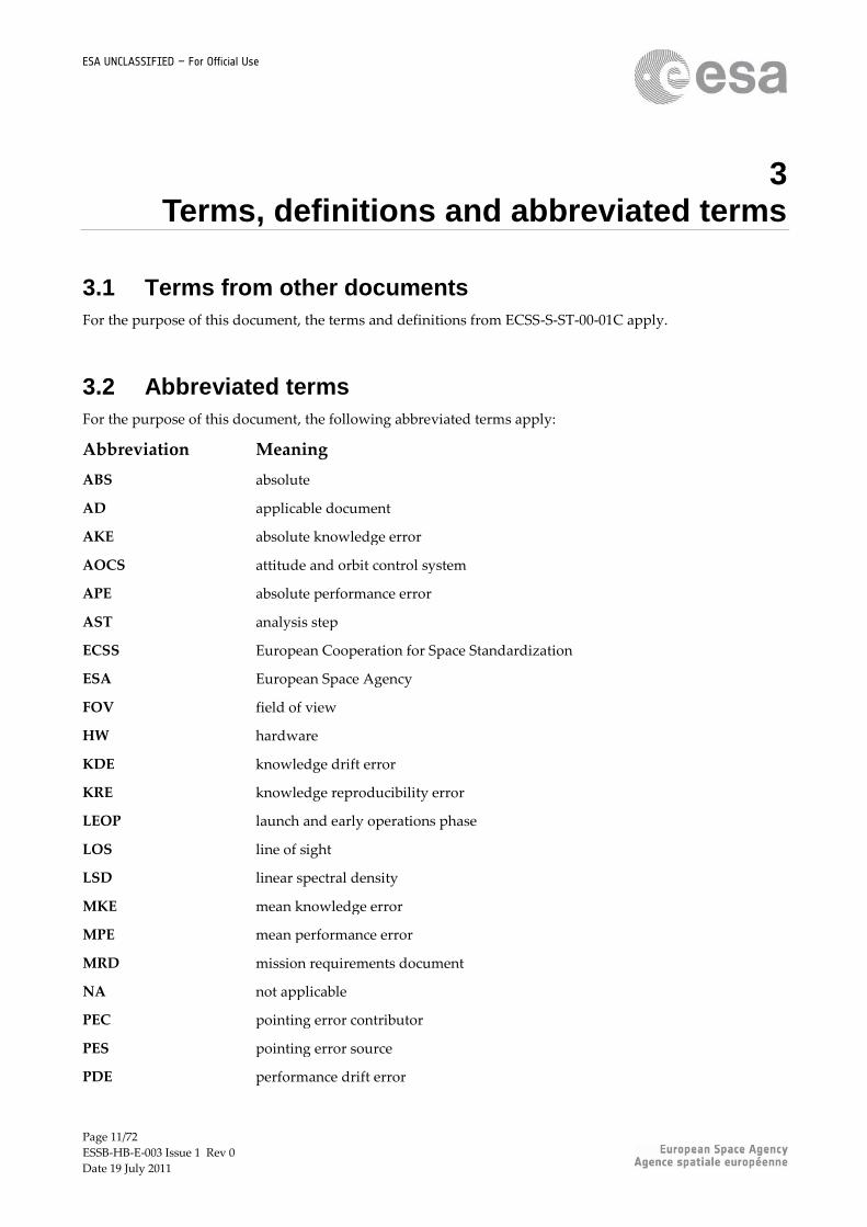
3.2 Abbreviated terms
For the purpose of this document, the following abbreviated terms apply:
Abbreviation Meaning
ABS absolute
AD applicable document
AKE absolute knowledge error
AOCS attitude and orbit control system
APE absolute performance error
AST analysis step
ECSS European Cooperation for Space Standardization
ESA European Space Agency
FOV field of view
HW hardware
KDE knowledge drift error
KRE knowledge reproducibility error
LEOP launch and early operations phase
LOS line of sight
LSD linear spectral density
MKE mean knowledge error
MPE mean performance error
MRD mission requirements document
NA not applicable
PEC pointing error contributor
PES pointing error source
PDE performance drift error

Page 12/72
ESSB-HB-E-003 Issue 1 Rev 0
Date 19 July 2011
ESA UNCLASSIFIED – For Official Use
PDF probability density function
PRE performance reproducibility error
PSD power spectral density
RD reference document
RKE relative knowledge error
RMS root mean square
RPE relative performance error
SS subsystem
STA stability
STR star tracker
SRD system requirements document
SW software
WM windowed mean
WMS windowed mean stability
WV windowed variance
3.3 Symbols
The following symbols are used in this handbook:
Symbol Meaning
... norm
time average
∆t window time
∆tD drift reset time interval
∆ts stability time
δ(…) Dirac-delta function
εindex zero mean pointing error per index (APE, RPE, …)
εD drift error
{...} Fourier transform
ℒ,…} Laplace transform
σ standard deviation
σBC , σCC standard deviation of time-constant PEC described as random variable
σCRP standard deviation of time-random PEC described as random process
σCR standard deviation of time-random PEC described as random variable
σSRP standard deviation of time-random PES described as random process

Page 13/72
ESSB-HB-E-003 Issue 1 Rev 0
Date 19 July 2011
ESA UNCLASSIFIED – For Official Use
σSC standard deviation of time-constant PES described as random variable
σSR standard deviation of time-random PES described as random variable
σ2 variance
µ mean value
µBC , µCC mean value of time-constant PEC described as random variable
µCRP mean value of time-random PEC described as random process
µCR mean value of time-random PEC described as random variable
µSRP mean value of time-random PES described as random process
µSC mean value of time-constant PES described as random variable
µSR mean value of time-random PES described as random variable
Ψ2 mean square value
A amplitude
B bias
BM(…) bimodal probability density function
C boundary on uniform distribution
Cee covariance function
D drift rate
E*…+ expected value of []
e(t) pointing error depending on time t
eindex pointing error per index
ec time-constant PEC
ec(t) time-random PEC
eK(t) pointing knowledge error
ek =e(k) pointing error depending on the ensemble realization index k
e(k,t) pointing error depending on the ensemble realization k and time t
ek(t) pointing error realization with index k
{ek(t)} ensemble of pointing error realizations ek(t)
eP(t) pointing performance error
er pointing error requirement
er,index pointing error requirement per index
es time-constant PES
es(t) time-random PES
Fmetric(ω,…) weighting function for time-windowed signal metric (ABS, WME, …)
,...)(~
sFmetric rational approximation of weighting function

Page 14/72
ESSB-HB-E-003 Issue 1 Rev 0
Date 19 July 2011
ESA UNCLASSIFIED – For Official Use
f frequency in [Hz]
fN Nyquist frequency in [Hz]
G(µ,σ) Gaussian probability density function
Gee(f) single-sided power spectral density in [unit2/Hz]
Gee(ω) single-sided power spectral density in [unit2/rad s-1]
H(jω) linear time-invariant transfer function
h(t) impulse response
k Index of specific ensemble realization
max*…+ maximum value of […]
min*…+ minimum value of […]
p(...) probability density function
p(...|...) probability density function depending on some event
pk(...) conditional probability density function depending on realization index k
pBC , pCC probability density function of time-constant PEC
pCR probability density function of time-random PEC
pSC probability density function of time-constant PES
pSR probability density function of time-random PES
P(…) probability distribution function
Pee linear spectral density
Pc level of confidence
U(..., ...) uniform probability density function
R(... ,...) Rayleigh probability density function
Ree autocorrelation function
See double-sided power spectral density
ω frequency in [rad/s]
Page 15/72
ESSB-HB-E-003 Issue 1 Rev 0
Date 19 July 2011
ESA UNCLASSIFIED – For Official Use
4 Pointing error: from sources to system
performance
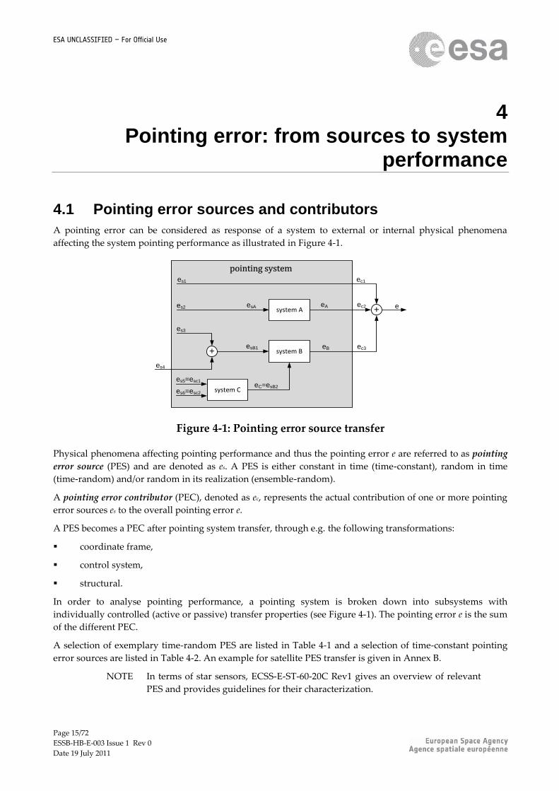
4.1 Pointing error sources and contributors
A pointing error can be considered as response of a system to external or internal physical phenomena
affecting the system pointing performance as illustrated in Figure 4-1.
system A
pointing system
+ e
system B+esB1
system C
ec1
eA ec2
eB ec3
eC=esB2
es2
es3
es5=esc1
es1
es4
es6=esc2
esA
Figure 4-1: Pointing error source transfer
Physical phenomena affecting pointing performance and thus the pointing error e are referred to as pointing
error source (PES) and are denoted as es. A PES is either constant in time (time-constant), random in time
(time-random) and/or random in its realization (ensemble-random).
A pointing error contributor (PEC), denoted as ec, represents the actual contribution of one or more pointing
error sources es to the overall pointing error e.
A PES becomes a PEC after pointing system transfer, through e.g. the following transformations:
coordinate frame,
control system,
structural.
In order to analyse pointing performance, a pointing system is broken down into subsystems with
individually controlled (active or passive) transfer properties (see Figure 4-1). The pointing error e is the sum
of the different PEC.
A selection of exemplary time-random PES are listed in Table 4-1 and a selection of time-constant pointing
error sources are listed in Table 4-2. An example for satellite PES transfer is given in Annex B.
NOTE In terms of star sensors, ECSS-E-ST-60-20C Rev1 gives an overview of relevant
PES and provides guidelines for their characterization.
Page 16/72
ESSB-HB-E-003 Issue 1 Rev 0
Date 19 July 2011
ESA UNCLASSIFIED – For Official Use
Table 4-1: Time-random PES
time-random PES – es(t)
Environmental disturbances (e.g. solar pressure noise)
Payload intrinsic error sources (e.g. optical filter wheel, cryogenic cooler)
Drive mechanisms (e.g. solar array, instrument, antenna, filter wheel)
Actuator intrinsic error sources (e.g. reaction wheel imbalances, thrusters noise)
Sensor bias and noise (e.g. star tracker, gyro, accelerometer, metrology, GPS)
Structure thermo-mechanical deformations (e.g. due to orbiting)
System dynamics induced errors (e.g. sloshing, flexible modes)
Table 4-2: Time-constant PES
time-constant PES - es
Misalignments (e.g. payload, sensor, etc.)
Calibration uncertainty (e.g. sensor bias)
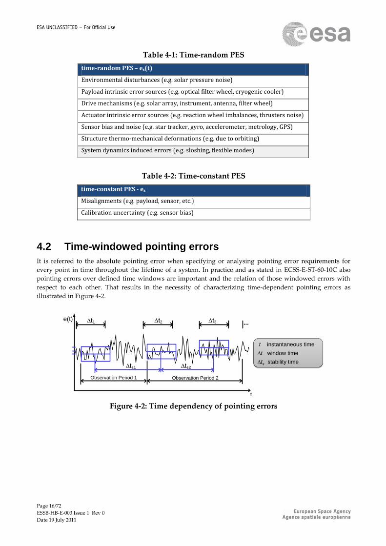
4.2 Time-windowed pointing errors
It is referred to the absolute pointing error when specifying or analysing pointing error requirements for
every point in time throughout the lifetime of a system. In practice and as stated in ECSS-E-ST-60-10C also
pointing errors over defined time windows are important and the relation of those windowed errors with
respect to each other. That results in the necessity of characterizing time-dependent pointing errors as
illustrated in Figure 4-2.
t
e(t)
∆t1
Observation Period 1 Observation Period 2
...∆t2 ∆t3
∆ts2∆ts1
t instantaneous time
∆t window time
∆ts stability time
Figure 4-2: Time dependency of pointing errors
Page 17/72
ESSB-HB-E-003 Issue 1 Rev 0
Date 19 July 2011
ESA UNCLASSIFIED – For Official Use
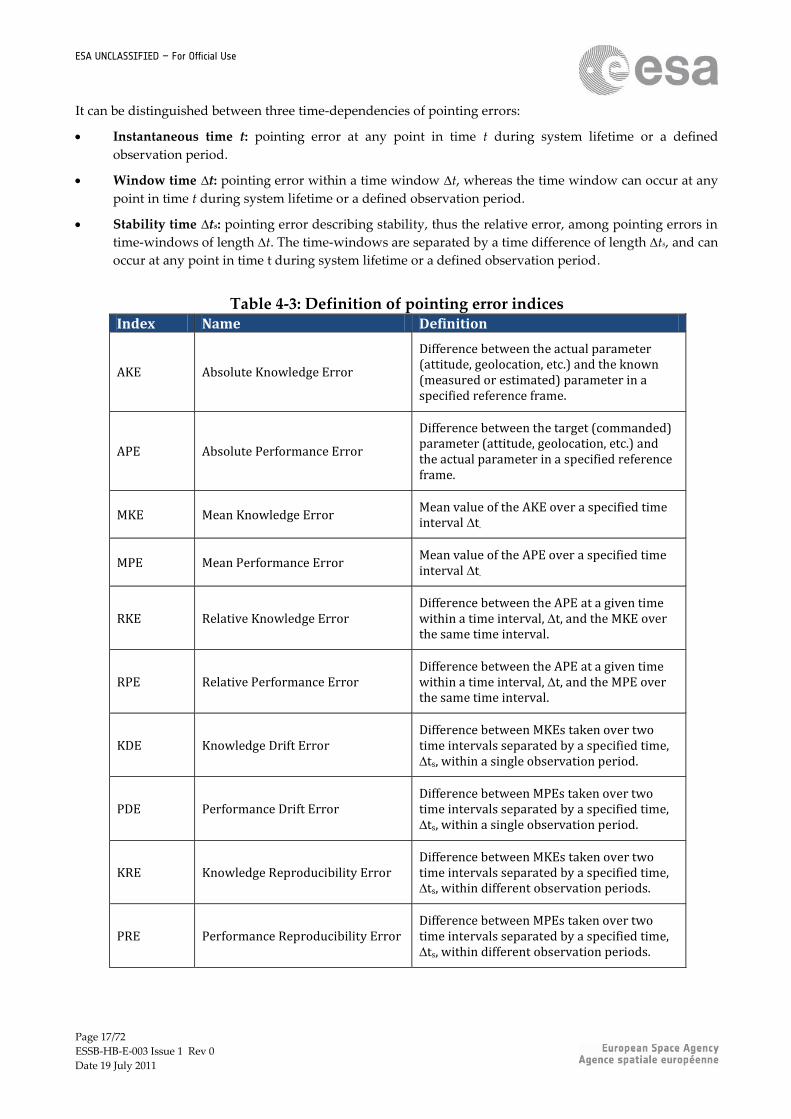
It can be distinguished between three time-dependencies of pointing errors:
Instantaneous time t: pointing error at any point in time t during system lifetime or a defined
observation period.
Window time ∆t: pointing error within a time window ∆t, whereas the time window can occur at any
point in time t during system lifetime or a defined observation period.
Stability time ∆ts: pointing error describing stability, thus the relative error, among pointing errors in
time-windows of length ∆t. The time-windows are separated by a time difference of length ∆ts, and can
occur at any point in time t during system lifetime or a defined observation period.
Table 4-3: Definition of pointing error indices Index Name Definition
AKE Absolute Knowledge Error
Difference between the actual parameter (attitude, geolocation, etc.) and the known (measured or estimated) parameter in a specified reference frame.
APE Absolute Performance Error
Difference between the target (commanded) parameter (attitude, geolocation, etc.) and the actual parameter in a specified reference frame.
MKE Mean Knowledge Error Mean value of the AKE over a specified time interval ∆t.
MPE Mean Performance Error Mean value of the APE over a specified time interval ∆t.
RKE Relative Knowledge Error Difference between the APE at a given time within a time interval, ∆t, and the MKE over the same time interval.
RPE Relative Performance Error Difference between the APE at a given time within a time interval, ∆t, and the MPE over the same time interval.
KDE Knowledge Drift Error Difference between MKEs taken over two time intervals separated by a specified time, ∆ts, within a single observation period.
PDE Performance Drift Error Difference between MPEs taken over two time intervals separated by a specified time, ∆ts, within a single observation period.
KRE Knowledge Reproducibility Error Difference between MKEs taken over two time intervals separated by a specified time, ∆ts, within different observation periods.
PRE Performance Reproducibility Error Difference between MPEs taken over two time intervals separated by a specified time, ∆ts, within different observation periods.

Page 18/72
ESSB-HB-E-003 Issue 1 Rev 0
Date 19 July 2011
ESA UNCLASSIFIED – For Official Use
The time-dependent pointing errors are defined in ECSS-E-ST-60-10C and summarized in Table 4-3. Note
that a KDE and KRE pointing error index is added in this handbook for being complete.
The comprehensive set of pointing error indices, categorized in knowledge or performance errors and
depending on instantaneous, window and stability time, is formulated in Table 4-4.
NOTE The necessity of analysing time-dependent pointing errors has its origin in
actual instrument and observation requirements of pointing systems, e.g. a
satellite and its payload, as discussed in [RD-01] and [RD-02].
Table 4-4: Mathematical formulation of pointing error indices
instantaneous time
window time
stability time
Pointing Error Indices
index instantaneous
eAPE(t) )(teP
eAKE(t) )(teK
eMPE(t, ∆t) ),( tteP
eMKE(t, ∆t) ),( tteK
eRPE(t, ∆t) ),()( ttete PP
eRKE(t, ∆t) ),()( ttete KK
ePDE(t, ∆t1, ∆t2, ∆ts) ePRE(t, ∆t1, ∆t2, ∆ts)
),(),( 21 tttette sPP
eKDE(t, ∆t1, ∆t2, ∆ts) eKRE(t, ∆t1, ∆t2, ∆ts)
),(),( 21 tttette sKK
st stability time
st stability time
indexe
instantaneous error
)(teK knowledge error signal
)(teP performance error signal
time average: dttet
tette
tt
tt
t
2/
2/
)(1
)(),(

Page 19/72
ESSB-HB-E-003 Issue 1 Rev 0
Date 19 July 2011
ESA UNCLASSIFIED – For Official Use
5 Pointing error engineering framework
5.1 Overview
Pointing error engineering covers the engineering process of establishing system pointing error
requirements, their systematic analysis throughout the design process, and eventually compliance
verification. In terms of specification, analysis and verification, it is necessary to be aware of the whole
pointing error engineering cycle. That is, for specification of pointing error requirements relevant analysis
and verification methods need to be identified and vice versa.
5.2 Methodology
The flow diagram in Figure 5-1 gives a schematic overview. The process starts with mapping Application
Requirements, as specified by the user, into System Pointing Error Requirements. The System Pointing Error
Requirements preferably follow the classification provided in Table 4-4. The compliance of the system
pointing error requirements is analysed by estimating and combining the different occurring error sources in
the analysis steps (AST) 1 to 4.
NOTE The mapping process is not further treated in this handbook because it is
application specific. However, in the future it is intended to provide a document
with exemplary requirement mapping cases for different types of satellite
missions. Apart from that, this handbook covers the whole pointing error
engineering cycle providing a framework with mathematical elements,
engineering methods and conventions.
As discussed in section 4 each subsystem (SS) within the pointing system is analysed in terms of their
Pointing Error Source (PES) transfer characteristics to compile a pointing error budget. Hence, the first
analysis step, AST-1, in pointing error analysis is to identify and characterize the PES.
In the second analysis step, AST-2, it is analysed how the different PES contribute to the pointing error, as
already mentioned in section 4. These Pointing Error Contributors (PEC) are obtained by a transformation,
which depends on the system under evaluation. The transformation can for example be a change in reference
frame. The transfer can also be a dynamic process, such as a satellite AOCS. The transfer characteristics of
each system are tuneable to a certain extent and thus can be used to perform trade-offs with the aim of
making pointing errors compliant with their requirement. AST-2 is elaborated in section 9.

Page 20/72
ESSB-HB-E-003 Issue 1 Rev 0
Date 19 July 2011
ESA UNCLASSIFIED – For Official Use
PES Characterization
Application Pointing System
Compliance or Redefinition Request
Application Performance
Application Requirements
System Design
PEC
PES Transfer Analysis
AST-2
System Specifications
Error Index Contribution Analysis
AST-3
Compliance or Redefinition Request
Absolute & Time-Windowed PEC
System Pointing Error Evaluation
PES Characteristics
AST-1
AST-4
System Pointing Error Requirements per Index
System Pointing Errors per Index
Mapping
Mapping
Figure 5-1: Pointing error engineering methodology structure
In early mission phases some of the transfer characteristics might not be available thus step AST-2 can be
discarded and the system needs to be considered to transfer the PES one-to-one. That means PES migrate
directly to PEC. On the other hand, in late development phases detailed knowledge of complex transfer
characteristics might be available for time domain and frequency domain analysis. In the case of frequency
domain analysis, simplified linearized models of the transformation process may be derived, as introduced
in section 9.2.
The third step, AST-3, determines the contribution of the PEC to the pointing error indices. It is elaborated in
section 10.

Page 21/72
ESSB-HB-E-003 Issue 1 Rev 0
Date 19 July 2011
ESA UNCLASSIFIED – For Official Use
AST-3 can be skipped for random time-constant PES because it does not depend on time. Moreover, AST-3
can also be skipped for the analysis of the Absolute Pointing Error because it only depends on the
instantaneous time, and not on windowed or windowed stability time.
The fourth step, AST-4, compiles the absolute and different time-windowed pointing error contributors to
obtain an estimate of the overall pointing error, which is then compared with the requirement. The analysis
step is elaborated in section 11.
In complex cases, the pointing system can be broken down in several subsystems. The Analysis Steps (AST)
from Figure 5-1 can then be applied to each subsystem as shown in Figure 5-2 for the example of an AOCS
subsystem. The steps AST-1 to AST-4 are applied on each subsystem of the pointing system. At the end AST-
4 is performed again on pointing system level in order to compile and evaluate the overall pointing error
budget.
Control
Structure
Definition
System
Optimization
sensorsactuatorsprocessorsdynamics
AOCS Design
PES
Characteristics
PES
Characterization
AST-1
AOCS Pointing Error
Requ. per Index
Control System
Specifications
System
Characteristics
Compliance or
Redefinition Request
Break Down
and
Allocation
Compliance or
Redefinition Request
AOCS Pointing Error
Evaluation
AST-4
PEC per Pointing
Error Index
System Budget
Compilation
Pointing System AOCS
AST-4
AOCS Pointing Errors
per Index
System Pointing Error
Requ. per Index
System Pointing
Errors per Index
Controller
Synthesis
AOCS Analysis
Performance
Analysis
AST-2Other
Analysis (e.g.
stability)PEC
Error Index
Contribution Analysis
AST-3
Figure 5-2: Pointing error engineering in AOCS
In this handbook a framework to characterize PES and analyse their transfer behaviour is defined.
Thereafter, AST-1 to AST-4 are elaborated and guidelines are introduced.

Page 22/72
ESSB-HB-E-003 Issue 1 Rev 0
Date 19 July 2011
ESA UNCLASSIFIED – For Official Use
5.3 Framework elements
5.3.1 Overview
The framework elements are the ‚design language‛ for pointing error engineering. It is a consistent
mathematical framework to describe relevant properties of PES for analysing their system transfer and
eventually to quantify the overall pointing error indices. The framework consists of methods used in
probability theory to describe properties of random physical phenomena acting as PES.
5.3.2 Mathematical elements
5.3.2.1 Overview
Mathematical elements necessary to perform pointing error engineering are summarized and introduced in
this section 5.3.2. This includes random variables, probability functions and random process theory. A
comprehensive discussion of the topics is given in [RD-03].
5.3.2.2 Random variable
A pointing error has random unpredictable magnitudes, with all possible magnitude values making up the
sample space. The magnitude values can either vary randomly in time (time-random) or in the ensemble of
realizations (ensemble-random). The random error magnitudes thus represent a random variable taking on
real numbers between -∞ and ∞ associated to each error sample point in the sample space. The random
variable can either be:
e(k) thus depending on the realization k,
e(t) thus depending on the point in time t,
e(k,t) thus depending on both, the realization k and point in time t.
NOTE The notation e(k) is used to introduce random variables and probability. It
represents the case where e varies due to any random-property making up a
sample space with k realizations. If the random property is linked to time, then
this is explicitly denoted by replacing k with t. In the more complex case is the
dependency of the pointing error depends on both k and t, thus e(k,t).
5.3.2.3 Probability distribution and density function with statistical properties
5.3.2.3.1 Overview
In order to perform pointing error analysis the error sample space needs to be characterized. In that respect
probability functions are assigned to describe the error sample space and thus the random variable or
process, cf. [RD-03].
5.3.2.3.2 Probability Distribution Function
In the general case, the probability distribution function describes the probability that a pointing error e(k) is
less than a defined required error value er, meaning that e(k) < er. The probability assigned to the set of points
k in the sample space that satisfy the inequality are described by the probability distribution function:

Page 23/72
ESSB-HB-E-003 Issue 1 Rev 0
Date 19 July 2011
ESA UNCLASSIFIED – For Official Use
ree(k)P(e) Prob
(5-1)
with P(-∞) = 0 and P(∞) = 1.
5.3.2.3.3 Probability Density Function
In terms of pointing error analysis it is more convenient to work with probability density functions (PDF). If
a random variable has a continuous range of values, the PDF is defined to be the first order derivative of the
probability distribution function:
de
dP(e)p(e)
(5-2)
with
1p(e)de and p(e) ≥ 0.
NOTE The probability density function p(e) is permitted to represent a Dirac-delta
function.
5.3.2.3.4 Statistical Properties
Statistical properties describe the random variables and are a function of the underlying PDF. Concerning
this handbook three different properties are of interest, all defined by the expected value.
The mean value µe of e(k) is defined by:
p(e)deeE[e(k)]μe
(5-3)
The mean square value 2e of e(k) is defined by:
p(e)dee]E[e(k)ψe222
(5-4)
The variance 2e of e(k) is defined by:
p(e)de)μ(e])μE[(e(k)μψσ eeeee22222
(5-5)
The RMS value corresponds to: 2ermse
(5-6)
NOTE In terms of pointing error analysis the RMS value is usually considered with
zero-mean value. If this is the case, this should be clearly mentioned.
5.3.2.3.5 Summary of Statistical Properties with Respective PDF
There are various PDF for describing the sample space of a pointing error. However, it is practical to describe
a pointing error in line with the most common ones. In this respect a summary of statistical properties with
the respective PDF is given in Table 5-1.

Page 24/72
ESSB-HB-E-003 Issue 1 Rev 0
Date 19 July 2011
ESA UNCLASSIFIED – For Official Use
Table 5-1: Statistical properties with respective PDF
PDF p(e) μe σe
Discrete )( ee e 0
Uniform 0
,)(),(
maxmin
1minmaxmaxmin
otherwiseeee
eeeeU
2
maxmin eeU
12
minmax eeU
Bimodal
0
,)(-1
22
otherwiseAe
eAABM
0BM ABM
2
1
Gaussian
(normal)
2
2
2
)(exp
2
1),(
e
e
e
ee
eG
eG eG
Rayleigh
0
, 2
exp),(2
2
2
e
eeeR
RR
R
R
2
R
2
4
5.3.2.3.6 Conditional Probability
Conditional probability is used to describe errors that are random with respect to two dependent variables.
Thus randomness over the ensemble realizations k as well as in time t can be described.
The topic of conditional probability is summarized in ECSS-E-ST-60-10C and discussed in detail in [RD-03]
and [RD-04].
In this handbook a conditional PDF is denoted as:
dekpkepepk )()|()(
(5-7)
with the statistical properties µe(k) and σe(k) depending on the realization index k.
NOTE Instead of using conditional probability it is possible to describe a pointing error
as stationary random process, cf. section 5.3.2.4. However, in order to do so,
mixed statistical interpretation needs to be specified in the pointing error
requirement.
5.3.2.4 Random process
A random pointing error process {ek(t)} is an ensemble of k sampling function realizations that are random in
time t (time-random) and random in its ensemble of realizations (ensemble-random). The ensemble is the set
,…} of all realizations k of the random pointing error ek(t). The probability properties of a random process are
described by the ensemble statistical quantities (e.g. mean or variance) at fixed values of t, where ek(t) is a
random variable over the index k. In general, the statistical quantities are different at different times t. If the
statistical quantities are equal for all t the random process is said to be stationary. In this handbook, if
referred to random processes, it is implicitly assumed that it is stationary.
A time-random pointing error ek(t) with ensemble-random realizations k can be described as a stationary
random process if time series data of the respective PES is available, and the conditions stated in [RD-03], for
stationary random processes description, are fulfilled.

Page 25/72
ESSB-HB-E-003 Issue 1 Rev 0
Date 19 July 2011
ESA UNCLASSIFIED – For Official Use
A stationary random process is described by its PDF p(e). In practice most stationary random processes have
a Gaussian PDF and thus are completely defined by their mean value and covariance respectively:
deepeteE ke )()]([
(5-8)
22 )()]()([()( eeeekkee RteteEC
(5-9)
where the autocorrelation is defined as:
212121 ),()]()([()( dedeeepeeteteER kkee
(5-10)
with e1=ek(t) and e2=ek(t+τ). Note that the statistics are independent of t and that the covariance function Cee(τ)
represents the variance of the random process for τ=0.
A stationary random process is ergodic in case the ensemble probability characteristics can be determined by
time averages of arbitrary realizations k. In terms of mean value and covariance this means that:
T
kT
eee (t)dteT
(k) μμ(k)μ
0
1limth wi
(5-11)
T
kkT
ee
eeeeeeeee
τ)dt(t(t)eeT
(R
(k)μ(Rk)(C (Ck)(C
0
2
1lim)
), with),
(5-12)
If a stationary random pointing error process is ergodic, pointing error analysis can be simplified
because the probability characteristics can be determined based on one time series instead of an
ensemble of time series.
NOTE A random process is stationary if its PDF is not a function of time. This is
usually the case for time-invariant operational conditions. If the conditions
change throughout the lifetime of the pointing system, a quasi-stationary
process needs to be identified. Quasi stationary process can be determined via
worst case behaviour of the PES over a specified period of interest or its
statistical properties are described as random variables themselves. An
alternative approach is to require error source signals to have stationary
behaviour, e.g. by controlling operational conditions of the PES. For time-
random errors that have transient behaviour a non-stationary random process
description and analysis is inevitable, cf. [RD-03].
5.3.2.5 Power spectral density
The frequency domain characteristics of a random stationary process are described by means of its power
spectral density (PSD). This becomes important when considering time- windowed pointing errors because a
windowing in the time domain is equivalent to a low pass filtering in the frequency domain. This enables
mathematically exact analysis of time dependent pointing errors as introduced in section 10.
In the frequency domain the power of a signal is equivalent to the area underneath the even double-sided
power spectral density PSD function See:
dffGdffSdffSfSR eeeeeeeeeee
000
12 )()(2)()()0(
(5-13)
Page 26/72
ESSB-HB-E-003 Issue 1 Rev 0
Date 19 July 2011
ESA UNCLASSIFIED – For Official Use
where the mean square value corresponds to the autocorrelation function at its maximum, which occurs for
τ=0.
There are different notations for a PSD as can be seen in Eq. (5-13). The double-sided PSD is denoted as See,
the single-sided PSD as Gee, but both are in [unit2/Hz]. In some literature the square-root of the single-sided
PSD Pee=√Gee in *unit/√Hz)+, also called Linear Spectral Density (LSD), is used. In this handbook it is mainly
referred to the single-sided PSD, Gee.
NOTE If a zero-mean random stationary process is ergodic, its PDF can be
characterized only by the knowledge of its PSD because a zero-mean Gaussian
PDF only depends on σe.
5.3.3 Statistical interpretation in context of framework
5.3.3.1 Overview
The properties of physical phenomena, and thus the pointing errors and their sources, are described in terms
of their probability characteristics. To make clear which property and corresponding probability
characteristic is described, it is necessary to choose the statistical population by specifying one of the three
statistical interpretations introduced in ECSS-E-ST-60-10C:
mixed
ensemble
temporal
Each statistical interpretation requires the description of a different probability characteristic, representing a
different property of the pointing error and thus a different statistical population. Hence the statistical
interpretation needs to be specified in the requirement formulation such that analysis is performed in line
with it. In the following the statistical interpretations, which are defined in ECSS-E-ST-60-10C, are
summarized and put into context with the random variable description in section 5.3.2.2, by e(k,t), and the
random process description in section 5.3.2.4, by {ek(t)}.
A PES has probability characteristics owing to its randomness in time (time-random), randomness in its
ensemble of realizations (ensemble-random) or both. In a pointing system several PES are usually acting
with different probability characteristics, but pointing error requirements are defined in line with one
statistical interpretation. Hence, if a PES is time-random and ensemble-random worst case assumptions are
necessary for one or the other property to guarantee evaluation in line with the specified statistical
interpretation of the pointing error requirement. This is clarified in sections 5.3.3.2 to 5.3.3.4.
NOTE At the respective pointing error analysis steps shown in Figure 5-1, it is
important to express the PES, PEC and pointing error indices in terms of the
required statistical interpretation.
Page 27/72
ESSB-HB-E-003 Issue 1 Rev 0
Date 19 July 2011
ESA UNCLASSIFIED – For Official Use
5.3.3.2 Mixed interpretation
In the mixed interpretation one considers the probability P greater or equal to a level of confidence Pc such
that the ensemble of pointing error realizations {ek(t)} or e(k,t) is less than a required error value er in its
ensemble of realizations k and in time t:
crcrk PetkePete ),(Probor )(Prob
(5-14)
NOTE In the mixed interpretation it is required to choose the statistical population
such that the pointing error is described with respect to its ensemble-random
and time-random probability characteristics concurrently. The mixed
interpretation is equivalent to the ensemble or temporal interpretation if a PES
does not randomly vary in time (time-random) or over its ensemble of
realizations (ensemble-random) respectively.
5.3.3.3 Ensemble interpretation
In the ensemble interpretation the probability P greater or equal to a level of confidence Pc is considered,
such that a realization k of the ensemble of pointing error realizations {ek(t)} or e(k,t) is less than a required
error value er for all times t:
),(max)(or )(max)( with )(Prob maxmaxmax tkeketekePeket
kt
cr
(5-15)
NOTE In the ensemble interpretation it is not required to choose the statistical
population thus that the time-random properties of the pointing error are
described, but rather the maximum value in time of each realization k as stated
in Eq.(5-15). This corresponds to a description of the ensemble-random
probability characteristics.
The maximum value usually occurs at different points in time for each
realization of a PES with time-random properties. Hence ‘ensemble’ refers to the
group of maximum values of the pointing error realization ek(t) and not to the
magnitude distribution of a time-random error realization.
If a PES is time-constant, {ek(t)}=e(k) or e(k,t)=e(k), and then the maximum value
of one realization is constant.
5.3.3.4 Temporal interpretation
In the temporal interpretation the probability P greater or equal to a level of confidence Pc is considered, such
that the entire ensemble of pointing error realizations {ek(t)} or e(k,t), or just the worst case realization, with
realization index k, is less than a required error value er for a fraction of time t:
),(max)(or )(max)( with )(Prob maxmaxmax tketetetePetek
kk
cr
(5-16)
NOTE In the temporal interpretation it is not required to choose the statistical
population thus that the ensemble-random probability characteristics of a
pointing error are described, but rather the time-random. Hence, if the
realization of a pointing error is random, with the ensemble index k, the time-
random properties of its worst case realization k need to be described as stated
in Eq.(5-16).
Page 28/72
ESSB-HB-E-003 Issue 1 Rev 0
Date 19 July 2011
ESA UNCLASSIFIED – For Official Use
6 Pointing error requirement formulation
6.1 Overview
A pointing error requirement is the specification of probability that the system output of interest does not
deviate by more than a given amount from the target output with a level of confidence Pc. In this context a
pointing error can refer to the actual system deviation and thus performance, or the determination of the
actual deviation thus knowledge.
This section 6 outlines the required parameters for unambiguously defining pointing error requirements. In
this context the major terms of ECSS-E-ST-60-10C are recalled for clarification.
6.2 Specification parameters
The following parameters and formulations need to be specified to unambiguously define pointing error
requirements:
required error value er;
statistical interpretation: ensemble, temporal, mixed;
angular deviation per axis or half-cone angle deviation in respective pointing reference frame on
which the requirement is imposed;
error index to be constrained, cf. section 4.2:
− pointing performance error: APE, MPE, RPE, PDE, PRE, or
− pointing knowledge error: AKE, MKE, RKE, KDE, KRE;
window time Δt and/or stability time Δts except in case of APE and AKE;
evaluation period;
the level of confidence Pc thus that cindexrindex Pee ,Prob ;
optional: PSD requirement GR(f) within respective bandwidth, with the restriction of f > 0.
NOTE Pointing requirements specified as PSD function GR(f) are usually self-
contained, meaning that there is no need to specify other parameters.
Page 29/72
ESSB-HB-E-003 Issue 1 Rev 0
Date 19 July 2011
ESA UNCLASSIFIED – For Official Use
6.3 Notes on requirement specification parameters and formulations
6.3.1 Reference frame and axis
The pointing scene of a satellite is illustrated in Annex A. The pointing requirements are specified in terms of
half-cone angle deviations, in the following called Line-Of-Sight (LOS) error, or as rotational angle deviations
per axes of the pointing reference frame, cf. ECSS-E-ST-10-09C, in the following called axis error. In this
respect small angles are assumed thus that the attitude error has vector properties.
It is important to take special care when defining a pointing requirement per axes or LOS. This is illustrated
in this section. Consider a pointing error made up of individual errors per axis of the pointing system
reference frame:
)cos()( 0 tAtex , (6-1)
)sin()( 0 tAtey , (6-2)
0)( tez . (6-3)
If the total error e is taken as the quadratic sum of the individual errors, then the LOS error becomes:
AttAtetee ooyx )(sin)(cos)()( 2222 , (6-4)
which is typically given e.g. in case of a dominating nutation motion.
The LOS pointing error in this case only consists of a time-constant mean value and thus has no frequency
content for arbitrarily large A. This means that the PSD of the error is:
)()( 2 eeeG , (6-5)
although the pointing errors per axis would have a PSD according to Eq.(8-3), at the frequency ω0.
This means that in case of LOS pointing error specification, the analysis in terms of pointing error index
contribution, as introduced in section 10, would result in no contributions to indices being affected by
frequency content other than at ωo=0 rad/s, i.e. RPE, RKE, KDE, PDE, KRE, PRE.
On the other hand pointing error specification per axes would result in an analysis regarding the PSD as it is
specified in Eq.(8-3).
Thus, e.g. considering the situation of a ‚nutating satellite‛, care needs to be taken when specifying PSD
requirements on the LOS. The PSD of the LOS might be compliant with the requirement by considering the
error magnitude e only, but considering the pointing scene in Annex A the pointing error vector le rotates
on the target plane. If an instrument does PSD measurements along the LOS, it might encounter a
disturbance PSD due to the rotating pointing error vector, although the vector magnitude, and thus the LOS
pointing error e, is constant. This is e.g. the case if a PSD is computed from payload intensity measurements
of a CCD, which usually has non-uniform pixel sensitivity.
NOTE The guidelines in ECSS-E-ST-60-10C, section 4.2.4, need to be considered when
mapping a half-cone pointing error requirement (of e.g. a payload boresight)
into rotational error requirements per axes of the pointing reference frame.

Page 30/72
ESSB-HB-E-003 Issue 1 Rev 0
Date 19 July 2011
ESA UNCLASSIFIED – For Official Use
6.3.2 Pointing error indices
The pointing error e needs to be constrained with respect to its time interval of interest, hence window time
or windowed stability, depending on the respective satellite mission application requirements.
6.3.3 Statistical interpretation
The statistical population is chosen in line with the mission application needs according to the three different
statistical interpretations of section 5.3.: ensemble, temporal and mixed. Each interpretation requires the
description of a different probability characteristic, representing a different random property of the pointing
error as discussed in section 5.3.3.
It might be practicable to specify different interpretations with respect to time-random and time-constant
sources such that the description represents the required application properties.
NOTE If PES are either time-random or time-constant and not both, the mixed
statistical interpretation is equivalent to the ensemble interpretation for time-
constant PES and to the temporal interpretation for time-random PES. Thus the
mixed statistical interpretation is the suitable approach to express pointing
requirements in many satellite missions.
6.3.4 Evaluation period
The evaluation period needs to be specified because different operations might require different pointing
error requirements of the same index. Usually an evaluation period corresponds to a satellite operational
mode, like ‚science observation‛.
6.3.5 Level of confidence
As defined in section 6.2 all requirements have the common mathematical form:
cindexrindex Pee ,Prob
where the level of confidence is e.g.:
99.7% (general case) or if applicable 3 (Gaussian distribution)
95.5% (general case) or if applicable 2 (Gaussian distribution)
68.3% (general case) or if applicable 1 (Gaussian distribution).
The use of the ‘n x σ’ notation for expressing probabilities is restricted to the cases where the pointing error
PDF is approximately Gaussian.
For a Gaussian PDF the 95.5% (2) bound is twice as far from the mean as the 68.3% (1) bound, but this
relation does not hold for a general distribution. However, the assumption of Gaussian distribution is valid
for many cases in practice due to the central limit theorem, cf. [RD-03], which states that the distribution of
the sum of a large number of independent distributed random variables converges to a Gaussian
distribution.
NOTE The guidelines of section 4.2.4 in ECSS-E-ST-60-10C need to be regarded when
evaluating the level of confidence, because e.g. Gaussian distributed pointing
errors per reference frame axis make up a Rayleigh distributed pointing error
per LOS.
Page 31/72
ESSB-HB-E-003 Issue 1 Rev 0
Date 19 July 2011
ESA UNCLASSIFIED – For Official Use
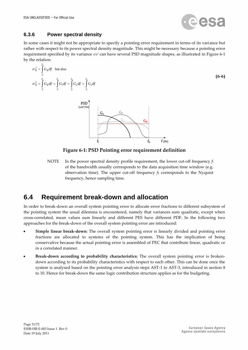
6.3.6 Power spectral density
In some cases it might not be appropriate to specify a pointing error requirement in terms of its variance but
rather with respect to its power spectral density magnitude. This might be necessary because a pointing error
requirement specified by its variance σR2 can have several PSD magnitude shapes, as illustrated in Figure 6-1
by the relation:
h
l
h
l
h
l
h
l
h
l
f
f
f
f
f
f
f
f
RR
f
f
RR
dfGdfGdfGdfG
dfG
3212
2 alsobut
(6-6)
f [Hz]fl fh
PSD[unit2/Hz]
GR
G1 G2
G3
Figure 6-1: PSD Pointing error requirement definition
NOTE In the power spectral density profile requirement, the lower cut-off frequency fl
of the bandwidth usually corresponds to the data acquisition time window (e.g.
observation time). The upper cut-off frequency fh corresponds to the Nyquist
frequency, hence sampling time.
6.4 Requirement break-down and allocation
In order to break-down an overall system pointing error to allocate error fractions to different subsystem of
the pointing system the usual dilemma is encountered, namely that variances sum quadratic, except when
cross-correlated, mean values sum linearly and different PES have different PDF. In the following two
approaches for the break-down of the overall system pointing error are introduced:
Simple linear break-down: The overall system pointing error is linearly divided and pointing error
fractions are allocated to systems of the pointing system. This has the implication of being
conservative because the actual pointing error is assembled of PEC that contribute linear, quadratic or
in a correlated manner.
Break-down according to probability characteristics: The overall system pointing error is broken-
down according to its probability characteristics with respect to each other. This can be done once the
system is analysed based on the pointing error analysis steps AST-1 to AST-3, introduced in section 8
to 10. Hence for break-down the same logic contribution structure applies as for the budgeting.

Page 32/72
ESSB-HB-E-003 Issue 1 Rev 0
Date 19 July 2011
ESA UNCLASSIFIED – For Official Use
7 Pointing error analysis methodology
7.1 Approach
An analysis methodology for establishing a pointing error budget is presented in this section 7. The pointing
error analysis methodology is adapted to the available PES data and tools as the pointing system design
matures. It is a combination of different mathematical elements, analysis methods and mainly two different
approaches:
frequency-domain approach: analytic approach restricted to Gaussian processes and linear time-
invariant systems to analyse characteristic error properties.
time-domain approach: based on numerical simulations and experimental results to analyse
characteristic error properties.
In general, separate pointing error budgets are made for different evaluation periods, e.g. spacecraft
operational modes. In this sense also nominal and exceptional budgets should be established. An exceptional
budget would for example include specific events like transients that affect the pointing performance in
relative short sporadic events. For distinguishing between exceptional and nominal, it is important to take
into account the likelihood of occurrence of the exceptional budget.
7.2 Methodology structure
The analysis methodology overall structure with intermediate analysis steps and results is illustrated in
Figure 7-1. It is in line with section 7.1, introduced approaches and consists of two different main analysis
methods:
a) simplified statistical method: analysis with variance, σ, and mean, μ, and their summation per ECSS
pointing error index under the assumption of the central limit theorem.
b) advanced statistical method: analysis by joint PDF characterization via convolution of different error
PDF, p…(e), as described in [RD-04], and evaluation of level of confidence for required ECSS pointing
error indices.
In Figure 7-1 method a) is depicted with solid lines whereas the advanced method is depicted as dashed
lines. Depending on the available data for the individual steps one or the other method or a combination is
applied. The indices letter ‘R’ in Figure 7-1 stands for random variable, the indices letters ‘RP’ stand for
random process, the index ‘index’ stands for the ECSS pointing error indices and the index letter ‘B’ stands
for bias.
Note that the analysis steps AST-1 to AST-4 are further elaborated and guidelines are introduced in section 8
to 11 of this handbook.

Page 33/72
ESSB-HB-E-003 Issue 1 Rev 0
Date 19 July 2011
ESA UNCLASSIFIED – For Official Use
σindex
μCR
σSR pSR
μindex
μSR
σCR
PES description: random variable
pCR
AST-2
AST-3
AST-4
B
error index contribution analysis
no → eS(t)eS ← yes
nth Pointing Error Source (PES)identification
for
n =
1 t
o N
time-constant
AST-1
transfer analysis
compilation of total pointing error per index
eRPE/RKEeMPE/MKEeAPE/AKE ePDE/KDE ePRE/KRE
nth PES error data eS
pSC
pBC
pCC
time-constant
time-random
μSCσSC
μCCσCC
σBC μBC
Gee
Gss
σCRP
σSRPpSRP
pCRP
transfer analysis
PES description: random variable
PES description: random process
RP-dataavailable
noyes
pN∗pN-1∗…∗p1pN∗pN-1∗…∗p1
εindex
Pc evaluation
pindex
ΣΣ Σ Σ
Pc evaluation
Figure 7-1: Pointing error analysis methodology overview

Page 34/72
ESSB-HB-E-003 Issue 1 Rev 0
Date 19 July 2011
ESA UNCLASSIFIED – For Official Use
8 Characterization of pointing error source:
AST-1
8.1 Overview
In order to describe and quantify properties for pointing error analysis, PES are analysed according to the
methodology in Figure 7-1, and in line with the framework elements in section 5.3. As outlined in Figure 8-1
the characterization of PES, denoted as Analysis Step AST-1, requires the identification of a PES, its
categorization in time-constant or time-random and its description as random variable or random process.
The handbook only provides guidelines for the description of PES error data because the PES identification is
case specific.
NOTE In Annex B examples are provided for different PES error types.
Inputs
Outputs
time-constant
time-random
σSR pSRμSR
PES description: random variable
no → eS(t)eS ← yes
nth Pointing Error Source (PES)identification
time-constant
nth PES error data eS
pSC μSCσSC Gss σSRPpSRP
PES description: random variable
PES description: random process
RP-dataavailable
noyes
Figure 8-1: Characterization method
8.2 Identification of pointing error source
The identification of characteristic PES error data is essential for a meaningful pointing error analysis. If no
detailed PES error data is available, assumptions based on experience need to be made to determine
equivalent error data necessary to describe the PES. However, as projects mature hardware for exact error
model identification should be made available.
The identification of PES is not subject of this handbook because case specific identification methods needs to
be applied, which can be found in literature, cf. [RD-03].

Page 35/72
ESSB-HB-E-003 Issue 1 Rev 0
Date 19 July 2011
ESA UNCLASSIFIED – For Official Use
8.3 PES error data classification
PES error data can be classified on the basis of characteristic signal properties as outlined in Figure 8-2. This
simplifies the description by the mathematical elements defined in section 5.3.2. If PES error data consists of
e.g. non-zero mean Gaussian noise, the data can be separated in two PES, the mean value and zero-mean
Gaussian noise error data content. Separating PES error data into signal classes structures and thus simplifies
analysis without loss of generality as explained in [RD-03]. This handbook as well as ECSS-E-ST-60-10C
provides guidelines for the characterization of bias, periodic, Gaussian random, uniform random and drift
error data. Transients and other random error data are usually system specific and thus are not treated in this
framework.
NOTE In this handbook a signal is defined as any measurable time-random and/or
ensemble-random physical phenomenon.
bias driftrandom
transient
deterministic
periodic otherGaussian uniform
PES error data
Figure 8-2: PES signal classes
The flow chart in Figure 8-3 provides guidelines for selecting eligible mathematical elements of section 5.3.2
to describe the signal-classified PES error data. As a first step it is distinguished between time-constant and
time-random data. This is a natural approach because the different pointing error indices are defined
according to time-windowed temporal pointing behaviour, see section 4.2. As shown in Figure 8-3 time-
constant PES error data corresponds to a bias that stays constant throughout all operational conditions.
Time-random PES error data is either random, periodic or a bias that changes its magnitude e.g. due to
different operational conditions.
NOTE A time-constant PES eS is constant in time and random with respect to its
ensemble of realizations. A time-random PES eS(t) is randomly varying in time
and can also be random with respect to its ensemble of realizations.
As a second step, it is distinguish whether the time-random PES error data is described by random process
theory or by a random variable. This depends on the availability of time series error data and if the random
process description criteria in [RD-03] are fulfilled.
The decision tree in Figure 8-3 provides guidelines for systematically selecting a suitable PES description
method. In the decision tree, the first criterion categorizes a PES in time-random and time-constant. Time-
constant PES do not vary randomly with time, but in their ensemble of realizations. On the other hand, time-
random PES have a magnitude that varies randomly in time and/or in its ensemble. A time-constant PES is
described as a random variable in line with section 5.3.2.2. A time-random PES is ideally described as a
stationary random process if time-series data is available and stationary random process theory is applicable.
Therefore guidelines for a stationary random process description are given in section 5.3.2.4. If time series
data is not available, ECSS-E-ST-60-10C provides guidelines for an approximate random variable description.
Note that describing a PES as stationary random process and thus characterizing its PSD has the advantage
that exact time window and stability time properties of the PES, as explained in section 10, are captured. This
approach is different compared to ECSS-E-ST-60-10C.

Page 36/72
ESSB-HB-E-003 Issue 1 Rev 0
Date 19 July 2011
ESA UNCLASSIFIED – For Official Use
guidelines in
E-ST-60-10C
guidelines in
ESSB-HB-E-003
guidelines in
E-ST-60-10C
eS ← yes time-
constant
PES error data eS
random variable random variable
RP-data
available
yes no
random process
no → eS(t)
Gaussian
→ LTI analysis
Bimodal
→ LTI analysis
Bias
Random
Bias(t)
Periodic
Random
Bias(t)
Random
Periodic
Uniform
Gaussian
other
other
Uniform
Gaussian
other
Figure 8-3: PES classification based on error data properties
As can be seen in Figure 8-3, periodic PES error data can also be described with random process theory, cf.
[RD-03]. In this respect one might argue that periodic PES error data is deterministic and thus has an exact
mathematical formulation. This is true if an exact characterization is possible and the temporal behaviour
predictable. In this case it indeed does not contribute to the pointing error because it can be compensated.
However, in practice an exact characterization is not always possible and thus clear boundaries between
random and deterministic cannot be drawn, i.e. a deterministic error signal might contain variables that take
on random values. A sine wave with a random distributed phase is such a signal, cf. [RD-03]. Hence also
random uncertainties in deterministic signals contribute to pointing errors.
8.4 Description of PES
8.4.1 Overview
The classification of PES error data is a systematic approach to identify suitable mathematical elements of
section 5.3.2 and ECSS-E-ST-60-10C for describing the error data. In the following section, for each case
shown in Figure 8-3, description guidelines are provided considering the statistical interpretation defined in
the pointing error requirement. Depending on the statistical interpretation, different probability
characteristics of the PES error data need to be described.
8.4.2 Time-constant PES description
A bias, which corresponds to a time-constant PES, can be the mean-content of a time-random PES or e.g. an
offset due to misalignment. The magnitude of a time-constant PES randomly varies with respect to its
ensemble of realizations. This means the bias is stable throughout the mission or varies only once as e.g. the
deviations experienced in the LEOP phase (launch vibrations, effect of gravity changes and initial thermal
distortions). In any case, during the operational phase of a mission, all these contributors have a constant
value for each pointing system (e.g. satellite) realization. They are compensated after in-flight calibration, so
only the residual bias is considered for the budgets established after in-flight calibration. Examples of bias-
type time-constant PES are given in Table 8-1.
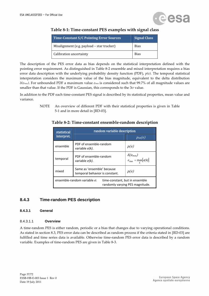
Page 37/72
ESSB-HB-E-003 Issue 1 Rev 0
Date 19 July 2011
ESA UNCLASSIFIED – For Official Use
Table 8-1: Time-constant PES examples with signal class
Time-Constant S/C Pointing Error Sources Signal Class
Misalignment (e.g. payload – star tracker) Bias
Calibration uncertainty Bias
The description of the PES error data as bias depends on the statistical interpretation defined with the
pointing error requirement. As distinguished in Table 8-2 ensemble and mixed interpretation requires a bias
error data description with the underlying probability density function (PDF), p(e). The temporal statistical
interpretation considers the maximum value of the bias magnitude, equivalent to the delta distribution
δ(emax). For unbounded PDF a maximum value emax is considered such that 99.7% of all magnitude values are
smaller than that value. If the PDF is Gaussian, this corresponds to the 3σ value.
In addition to the PDF each time-constant PES signal is described by its statistical properties, mean value and
variance.
NOTE An overview of different PDF with their statistical properties is given in Table
5-1 and in more detail in [RD-03].
Table 8-2: Time-constant ensemble-random description
statistical interpret.
random variable description
pSR(e)
ensemble PDF of ensemble-random variable e(k).
p(e)
temporal PDF of ensemble-random variable e(k).
δ(emax)
e(k)ek
maxmax
mixed Same as ‘ensemble’ because temporal behavior is constant.
p(e)
ensemble-random variable e: time-constant, but in ensemble randomly varying PES magnitude.
8.4.3 Time-random PES description
8.4.3.1 General
8.4.3.1.1 Overview
A time-random PES is either random, periodic or a bias that changes due to varying operational conditions.
As stated in section 8.3, PES error data can be described as random process if the criteria stated in [RD-03] are
fulfilled and time series data is available. Otherwise time-random PES error data is described by a random
variable. Examples of time-random PES are given in Table 8-3.
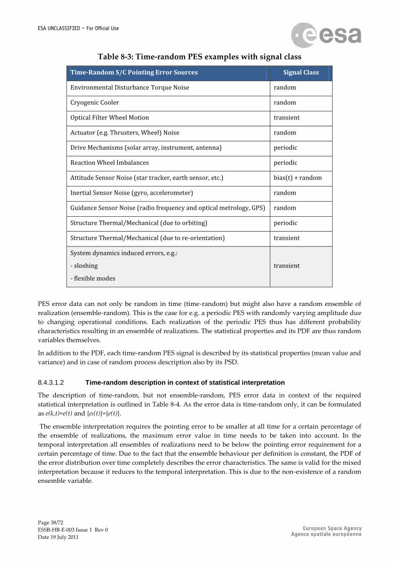
Page 38/72
ESSB-HB-E-003 Issue 1 Rev 0
Date 19 July 2011
ESA UNCLASSIFIED – For Official Use
Table 8-3: Time-random PES examples with signal class
Time-Random S/C Pointing Error Sources Signal Class
Environmental Disturbance Torque Noise random
Cryogenic Cooler random
Optical Filter Wheel Motion transient
Actuator (e.g. Thrusters, Wheel) Noise random
Drive Mechanisms (solar array, instrument, antenna) periodic
Reaction Wheel Imbalances periodic
Attitude Sensor Noise (star tracker, earth sensor, etc.) bias(t) + random
Inertial Sensor Noise (gyro, accelerometer) random
Guidance Sensor Noise (radio frequency and optical metrology, GPS) random
Structure Thermal/Mechanical (due to orbiting) periodic
Structure Thermal/Mechanical (due to re-orientation) transient
System dynamics induced errors, e.g.:
- sloshing
- flexible modes
transient
PES error data can not only be random in time (time-random) but might also have a random ensemble of
realization (ensemble-random). This is the case for e.g. a periodic PES with randomly varying amplitude due
to changing operational conditions. Each realization of the periodic PES thus has different probability
characteristics resulting in an ensemble of realizations. The statistical properties and its PDF are thus random
variables themselves.
In addition to the PDF, each time-random PES signal is described by its statistical properties (mean value and
variance) and in case of random process description also by its PSD.
8.4.3.1.2 Time-random description in context of statistical interpretation
The description of time-random, but not ensemble-random, PES error data in context of the required
statistical interpretation is outlined in Table 8-4. As the error data is time-random only, it can be formulated
as e(k,t)=e(t) and {ek(t)}={e(t)}.
The ensemble interpretation requires the pointing error to be smaller at all time for a certain percentage of
the ensemble of realizations, the maximum error value in time needs to be taken into account. In the
temporal interpretation all ensembles of realizations need to be below the pointing error requirement for a
certain percentage of time. Due to the fact that the ensemble behaviour per definition is constant, the PDF of
the error distribution over time completely describes the error characteristics. The same is valid for the mixed
interpretation because it reduces to the temporal interpretation. This is due to the non-existence of a random
ensemble variable.

Page 39/72
ESSB-HB-E-003 Issue 1 Rev 0
Date 19 July 2011
ESA UNCLASSIFIED – For Official Use
Table 8-4: Time-random description w.r.t. statistical interpretation
statistical interpret.
random variable description random-process description
pSR(e) pSRP(e)
ensemble Maximum value of time-random variable e(t).
δ(emax)
e(t)et
maxmax
Maximum value of time-random process {e(t)}.
δ(emax)
}{maxmax e(t)et
temporal PDF of time-random variable e(t).
p(e) PDF of time-random process {e(t)}.
p(e)
mixed
Same as ‘temporal’ because ensemble behavior is constant.
p(e)
Same as ‘temporal’ because ensemble behavior is constant.
p(e)
time-random variable e: in time randomly varying PES magnitude.
8.4.3.1.3 Time- and ensemble-random description in context of statistical interpretation
The description of time-random and ensemble-random PES error data in context of the required statistical
interpretation is outlined in Table 8-5. As the error data is time-random and ensemble-random, the random
variable, describing the PES data depends, on k and t, thus e(k,t). On the other hand, describing the PES data
as random process {ek(t)} requires stationary error data.
Ensemble interpretation requires that the pointing error is smaller at all time for a certain percentage of the
ensemble of realizations such that the ensemble PDF of the maximum error value emax needs to be taken into
account. In the temporal interpretation all ensembles of realizations need to be below the pointing error
requirement for a certain percentage of time. This corresponds to the worst case PDF describing the time-
random PES magnitude. The mixed interpretation requires a description by conditional probability in terms
of random variable description as stated in [RD-03] and ECSS-E-ST-60-10C, or simply by the PDF in terms of
stationary random process description.
NOTE If a PES is a non-stationary process that has varying statistical properties due to
e.g. different operational conditions, it might be described as stationary process
with random statistical properties, i.e. variance σe(k) and mean µe(k). Hence the
statistical properties of the random process would be random themselves and
described as variance of the random variance σσ and random mean µσ with the
conditional PDF, pk(e).

Page 40/72
ESSB-HB-E-003 Issue 1 Rev 0
Date 19 July 2011
ESA UNCLASSIFIED – For Official Use
Table 8-5: Time- and ensemble-random description w.r.t. statistical interpretation
statistical interpret.
random variable description random-process description
pSR(e) pSRP(e)
ensemble
PDF of random variable e(k,t) for worst case error w.r.t. time-random index t.
p(emax)
t)e(kket
,max)(max
PDF of maximum values in time for all realizations k of the stationary random process {ek(t)}.
p(emax)
}{max)(max (t)eke kt
temporal
PDF of random variable e(k,t) for worst case error w.r.t. ensemble-random index k.
p(emax)
t)e(ktek
,max)(max
PDF of worst case ensemble realization k of the stationary random process {ek(t)}.
p(emax)
}{max)(max (t)ete kk
mixed PDF of the random variable e(k,t).
pk(e)=
∫ p(e|k)p(k)de
PDF of stationary random process {ek(t)}.
p(e)
time-random variable e: in time randomly varying PES magnitude.
ensemble-random variable with index k: in ensemble randomly varying PDF of time-random variable e.
8.4.3.2 Random process PES description
8.4.3.2.1 Overview
The description of time-random PES error data by random process theory requires characterization of the
PDF and PSD. The PDF describes the likelihood of error magnitude occurrences throughout time, but not at
which time constants magnitude values occur. That means a PDF does not contain information for analysing
and quantifying time-windowed pointing errors. Characterizing the error source also by its PSD provides
information about time constants as the PSD describes power magnitude per frequency range. Thus, the PSD
of an error source is the basis for time-windowed pointing error analysis as is shown in section 10.
The PES error data is decomposed in mean value and zero-mean process to simplify analysis without loss of
generality. Depending on the temporal behaviour the mean values are treated as time-constant bias or time-
random bias.
8.4.3.2.2 Periodic
Periodic PES error data is a composition of sine functions, where each sine function stands for a single PES
and is described by its frequency f0, amplitude Ak and phase θ. If the phase θ of a single periodic PES is not or
cannot be predicted, it can be assumed to have a uniform PDF between ±π. The amplitude A can be a
random variable itself depending on the ensemble index k.
The periodic PES can thus be described as pseudo random process: tfAte kk 02sin()(
(8-1)
The random process is stationary (and ergodic) if the amplitude is considered to be equal for each k, meaning
that Ak = A. In this case the PDF is bimodal:

Page 41/72
ESSB-HB-E-003 Issue 1 Rev 0
Date 19 July 2011
ESA UNCLASSIFIED – For Official Use
0 otherwise , 1
)()(22
k
k
kk AeeA
ABMep
(8-2)
and pk(e) = p(e). If the amplitude Ak is random, pk(e) is also random with respect to the ensemble index k. In
this case the statistical properties, i.e. mean and standard deviation, are also random variables, µ=µ(k) and
σ=σ(k). For Ak=A Table 8-4 applies to determine a correct description of the PES in line with the statistical
interpretation defined in the pointing error requirement. Otherwise, meaning that the amplitude varies,
Table 8-5 applies.
The power spectral density (PSD) of periodic PES error data is described by:
)(2
)( 0
2
ffA
fGee
(8-3)
where δ(f-f0) is the Dirac-Delta function at the frequency f0 of the periodic PES.
8.4.3.2.3 Gaussian Random
Gaussian random PES error data is usually noise, which behaviour by definition is not predictable and thus
can only be described by random process theory, namely its probability characteristics and power spectral
density. There is no cross-correlation between successive realizations and it cannot be decomposed in
elementary single periodic errors. Those errors usually originate from actuation noise or sensor
measurements as can be seen in Table 4-1.
An ergodic stationary Gaussian random process {e(t)} with zero-mean value is completely described by its
variance:
dffG
TfordtteT
eepwithdeepeteE
ee
T
e
ee
)(
)(1
]2
exp[)2()()()]([
0
2
2
21222
(8-4)
It should be noted that the PSD of a PES can have any shape, meaning that the noise can be time-correlated.
NOTE If the PSD Gee of a PES is not available, but only its variance σe2, a first
approximation would be to assume the PSD of band-limited white noise with a
magnitude of Gee = σe2/fN with fN being the Nyquist frequency of e.g. sensor noise.
8.4.3.3 Random variable PES description
8.4.3.3.1 Bias(t)
A bias can be the mean-content of a time-random PES or any other offset like the misalignment of structural
parts. The time-random bias is time-constant at the timescale of an observation period, but its value can vary
randomly at the scale of the pointing system (e.g. satellite) lifetime. This is due to a change in operational
conditions, e.g. external influences like temperature and attitude, and not due to time-windowed temporal
signal properties. Thus it is possible to have a bias which is constant during one observation, but changes
between two different observations. For example, an attitude dependent star sensor error is constant as long
as the sensor sees the same area of the sky, but varies when its orientation changes.

Page 42/72
ESSB-HB-E-003 Issue 1 Rev 0
Date 19 July 2011
ESA UNCLASSIFIED – For Official Use
The PES error data, that represents a time-random bias, is described as random variable by any PDF and
their statistical properties, which are summarized in section 5.3.2 and can be found in [RD-03].
NOTE Time-random behaviour of a PES mean value considered during an observation
window Δt is not described by the bias signal class. The random variable
description of a bias is necessary if the random changes in the mean value occur
based on non-stationary behaviour of the time-random PES.
8.4.3.3.2 Uniform Random
Uniform time-random PES error data varies over short timescale, with a uniform PDF in a given range with
maximum value C, i.e. there is zero probability that an error occurs outside this range. Such errors usually
originate in quantisation of a signal, e.g. analogue-to-digital converter resolution errors or errors from a
bang-bang controller.
The time-random bias PES error data is described as random variable by a uniform distribution:
otherwise
CeC
ep
ep
0
0
)(
)( 1
(8-5)
with the statistical properties, namely variance and mean:
12
22 Ce
(8-6)
2
Ce
(8-7)
8.4.3.3.3 Transient
Transient time-random PES error data is from short-duration non-stationary phenomena with a clearly
defined beginning and end, cf. [RD-03]. The error data has complex temporal evolution (e.g. transient
oscillations due to moving parts such as rotating mirrors) which cannot be classified in any of the other
categories, even after subdivision in elementary error sources.
Depending on the application it might eventually be necessary to specify time requirements for transients to
reach stationary conditions due to their temporal limited appearance as it is the case for e.g. transients during
re-pointing. In this respect one would define transition periods from stationary to stationary behaviour,
rather than including transient-type errors in the budget. Hence a mission and error data specific description
method needs to be identified for any PES error data determined to have transient behaviour.
NOTE Henceforth no specific guidelines are provided for transient data within the
general pointing engineering framework of this handbook. However to avoid
excessive contributions to budgets, it may be desirable to produce two separate
budgets: one with (nominal budget) and one without transient contributions
(exceptional budget). In some cases two separate sets of requirements may be
given for nominal and exceptional performance.

Page 43/72
ESSB-HB-E-003 Issue 1 Rev 0
Date 19 July 2011
ESA UNCLASSIFIED – For Official Use
8.4.3.3.4 Drift
Time-random PES error data that varies approximately linearly with time is called drift. The origin is usually
a mean or random error integrated over time and thus does not truly represent a separate signal class in the
mathematical sense. However in terms of pointing error analysis a separate categorization simplifies
analysis.
As stated in [RD-04] a drift error has a linear variation with time:
DD tD
(8-8)
where D is the drift rate in [unit/s]. It is assumed that the drift is reset at intervals ΔtD (e.g. after each
observation). Depending on the context, the drift rate D may be a single value, a worst case or an ensemble
parameter.
In [RD-04] guidelines are provided for describing drift-type time-random errors as random variables.

Page 44/72
ESSB-HB-E-003 Issue 1 Rev 0
Date 19 July 2011
ESA UNCLASSIFIED – For Official Use
9 Transfer analysis: AST-2
9.1 Overview
The description of the PES is given with respect to its point of origin. In order to evaluate a pointing error
requirement the transfer of a PES from its origin to the point of interest needs to be analysed to determine the
pointing error contributor (PEC). In this context transfer analysis refers to reference frame coordinate
transformations as described in ECSS-E-ST-10-09C and to system transformations, e.g. AOCS closed-loop
sensor noise transformation. This handbook concentrates on system transformations.
Inputs
OutputsμCR
σSR pSRμSR
σCR pCR
transfer analysis
pSC
pCC
μSCσSC
μCCσCC Gee
GSS
σCRP
σSRPpSRP
pCRP
transfer analysis
time-constant
time-random
Figure 9-1: Transfer analysis
The input (PES) and output (PEC) parameters of the transfer analysis are shown in Figure 9-1. In the
following section an approach for system transfer analysis is introduced that relies on random process
theory. Different techniques in frequency and time domain exist for system transformation of time-random
PES described as random processes. It can be distinguished between analytic methods, which are based on
linear transformation of statistical properties, and numerical methods, which rely on simulations and
experimental results.
The system transfer of a PES described as random variables needs to be analysed case by case and cannot be
described in a general approach. The payload-star tracker misalignment error would be an example for this
case. However, in most cases of random variable description the PES directly corresponds to the PEC and
system transfer analysis is not required, except for coordinate transformations.
Time-constant PES system transformation analysis is a simple multiplication of the bias/mean value with the
system DC-gain.
NOTE It is recommended to express PEC per axis of a common pointing requirement
reference frame in terms of the rotation angle errors: ex, ey, ez or as directional
half-cone errors considering the constraints described in section 6.2.

Page 45/72
ESSB-HB-E-003 Issue 1 Rev 0
Date 19 July 2011
ESA UNCLASSIFIED – For Official Use
9.2 Frequency-domain
The transfer analysis is concerned with the input-output relation of a system, as comprehensively discussed
in [RD-03] and [RD-05]. If the input error signal of a system, the PES, is known and the system can be
represented by a linear time-invariant (LTI) transfer function H(jω), being stable and strictly proper, the
output error signal, the PEC, can be determined.
According to Eq.(5-13) the variance of a PES described as random processes is related to its PSD by:
dGe ssSRP
0
2 )(2
1)(
(9-1)
The PSD Gss of the input error signal es(t) is transformed by the system according to the relation, cf. [RD-03]:
)()()(2
ssee GjHG
(9-2)
The variance of the output error signal ec(t) is thus computed from its PSD Gee by:
dGeeCRP
0
2 )(2
1
(9-3)
The transfer of the PES variance can also be analysed by state-space methods as introduced in [RD-05]. The
PES is modelled as the covariance matrix of a Gaussian white noise process with a spectral form filter in
state-space representation. With the system transfer matrix the PEC can thus be computed with linear
algebra methods.
In order to tune the system transfer function H(jω) and to quantify pointing errors, signal and system norms are
advantageous. They are introduced in Annex C. In [RD-06] pointing error index specific signal norms are
introduced based on [RD-01], [RD-02], and [RD-05] in order to tune closed loop control systems, e.g. the AOCS.
NOTE In terms of analysing the system transfer of a PES, being an ergodic stationary
random process with Gaussian distribution, it is only necessary to analyse the
PSD transfer because: Gaussian PDF at system input is equal to Gaussian PDF at
system output. The same applies if the PES is a periodic pseudo stationary
random process.
9.3 Time-domain
In order to analyse the error transfer from the PES to the actual pointing error, time-domain simulations can
be run instead of analytic frequency-domain analyses. The described PES PDF (e.g. uniform, Gaussian,
bimodal distribution) or PSD in terms of random processes are used to model PES behaviour. Then time-
domain simulations are run to get sufficient error sample size, which is statistically representative for
characterizing the pointing error contributor PEC at the system output of interest. Each or a joint PEC is then
again characterized with respect to its PDF in form of a cumulative histogram and by their PSD.
The topic of simulations is treated in more detail in [RD-04].
NOTE Transfer analysis by simulations does not provide a systematic design
framework as the methods used in the analytic analysis. However they are
inevitable for system performance verification in terms of Monte-Carlo
Simulations.

Page 46/72
ESSB-HB-E-003 Issue 1 Rev 0
Date 19 July 2011
ESA UNCLASSIFIED – For Official Use
10 Pointing error index contribution: AST-3
10.1 Overview
Depending on the description of the PES in AST-1 different approaches need to be chosen for the time-
windowed pointing error index contribution analysis in line with the pointing error indices defined in
section 4.2. The separation of time-random and time-constant PES in AST-1 is actually because of the time-
windowed error index contribution analysis described in this section 10. The contribution analysis is shown
in Figure 10-1 with input and output parameters.
Inputs
Outputsσindex
μCR
μindex
σCR pCR
error index contribution analysis
pBC
pCC μCCσCC
σBC μBC
Gee σCRPpCRP
pindex
time-constant
time-random
Figure 10-1: Pointing error index contribution analysis
It is not necessary to analyse time-constant PEC because they are by definition independent of time. On the
other hand, time-random PEC need to be analysed since their contribution depends on the time window
length, Δt and Δts.
The random variable description of time-random PES does not include information about time-constants in
the error signal because it is only described by its PDF. Nevertheless, in most cases such errors have discrete
time changes, meaning that their magnitude change is correlated with a known event. An example would be
the attitude-dependent bias of a star tracker. In this case one knows that the bias changes from one
observation period with respect to the other, which results in a stability PEC in the PDE or PRE index. Hence,
it is important to analyse the statistical properties, quantifying the error index contribution of a PEC
described as random variable, case by case. In this respect ECSS-E-ST-60-10C and [RD-04] provide guidelines
for different error PDF.
The description of time-random PES as random processes includes information about the temporal
behaviour of the PES in form of the PSD. The pointing error index contribution of such a PEC can be
quantified by time-windowed PSD metrics, in the following referred to as pointing error metrics.
NOTE In order to analyse a time-random PES with random process theory the PES
data needs to be stationary such that its statistic properties are time-invariant. In
this case the metric definitions represent a signal norm, cf. [RD-05]. Moreover,

Page 47/72
ESSB-HB-E-003 Issue 1 Rev 0
Date 19 July 2011
ESA UNCLASSIFIED – For Official Use
in order to completely determine the pointing error PDF, the stationary random
process needs to be ergodic as mentioned in section 5.3.2.4.
10.2 Worst case pointing error index
The worst case pointing error indices are defined for the instantaneous pointing errors in Table 4-4. This is
necessary if a requirement has different window times and instead of performing analysis for all window
times, only the worst case window time is analysed.
Unlike in Table 10-1 in the following it is not distinguished between knowledge error eK and performance
error eP because for the time-windowed analysis the describing metrics are the same.
Table 10-1: Worst case pointing error index
Pointing Error Indices index instantaneous worst case
eAPE(t) )(teP not applicable
eAKE(t) )(teK not applicable
eMPE(t, ∆t) ),( tteP ),( mintteP
eMKE(t, ∆t) ),( tteK ),( mintteK
eRPE(t, ∆t) ),()( ttete PP ),( maxtteP
eRKE(t, ∆t) ),()( ttete KK ),( maxtteK
ePDE(t, ∆t1, ∆t2, ∆ts) ePRE(t, ∆t1, ∆t2, ∆ts)
),(),( 32 tttette sPP minmin
)()( max, tsPtP ttete
eKDE(t, ∆t1, ∆t2, ∆ts) eKRE(t, ∆t1, ∆t2, ∆ts)
),(),( 21 tttette sKK minmin
)()( max, tsKtK ttete
st stability time where: ∆ts, max = max[∆ts].
t window time where: ∆tmin = min[∆t], ∆tmax = max[∆t].
with ∆t=∆t1=∆t2
indexe
instantaneous error
)(teK knowledge error signal
)(teP performance error signal
time average: dttet
tette
tt
tt
t
2/
2/
)(1
)(),(
The PDE and PRE errors cannot be described by time-windowed metrics in a mathematical sense. Time-
windowed metrics only exist for a constant window evaluation time Δt as shown in Figure 10-2 and a
constant stability evaluation time Δts=ΔtPDE/PRE defined by the time difference of two window centres.
However, if there are changing window times for pointing observations, which need to be compared in
terms of their stability, one can make an upper bound evaluation according to the worst case MPE window
time Δt, corresponding to min*Δt+, and the worst case stability time max*Δts]. This becomes illustrative
considering the time-windowed metric weighting functions in Table 10-3.
NOTE The mathematical definitions of PDE and PRE (seeTable 10-1) are identical. As
indicated in Note 5 of section 3.2.10 in ECSS-E-ST-60-10C the difference is in the
use of these error indices. The PDE is used to quantify stability among two

Page 48/72
ESSB-HB-E-003 Issue 1 Rev 0
Date 19 July 2011
ESA UNCLASSIFIED – For Official Use
points in time, which are apart a defined time Δts=ΔtPDE. The PRE expresses the
same stability with Δts=ΔtPRE, but among different defined periods, e.g.
observation periods.
PD
E(Δ
t 1,
Δt P
DE)
time t
e
MPE obs1(Δt1)
Observation period 1 Observation period 2
PRE(Δt1, ΔtPRE)
MPE obs2(Δt1)
Δt1 Δt1
Δts=ΔtPDE Δts=ΔtPRE
Δt1
Figure 10-2: PDE/PRE pointing metrics interpretation
10.3 Pointing error metrics
10.3.1 Overview
The time windowed pointing error metrics, derived in [RD-01] and [RD-02], are summarized in Table 10-2.
The metrics correspond to different pointing error indices. The absolute, windowed and windowed mean
mapping of metrics to indices is straight forward considering the instantaneous worst case error definitions
in Table 10-1. Stability and windowed mean stability describe the same set of indices, this is due to the fact
that stability is a special case of windowed stability, namely for Δt = 0. Nonetheless, the stability metrics are
listed in Table 10-2 to be complete.
The metrics are computed by evaluating the integrals of the PEC PSD of the zero-mean stationary random
process. Note that the zero-mean property of the error is emphasized by including the absolute error signal
mean value, µABS, in the metrics in Table 10-2.
NOTE 1 In Annex D some notes are provided on the stability and windowed-
stability pointing error metric.
NOTE 2 The expected value E[…] in Table 10-2 is computed via the time average
if the stationary pointing error process is ergodic. Otherwise it needs to be
computed via the ensemble average, cf. [RD-03].
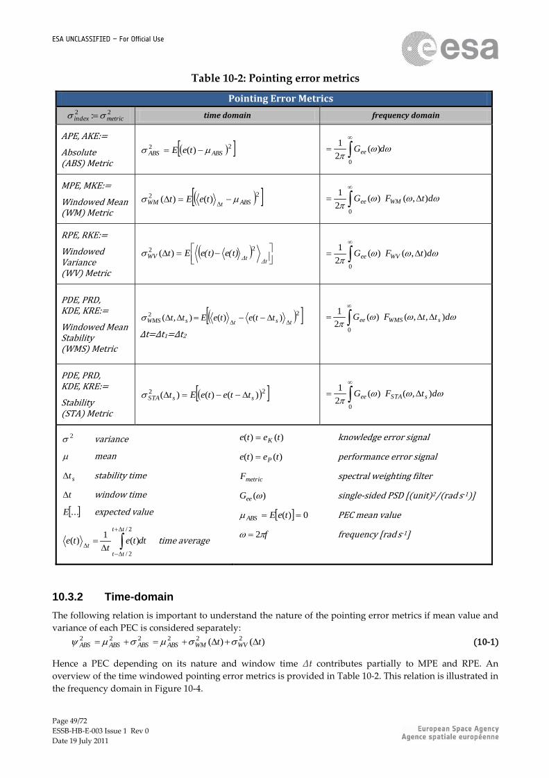
Page 49/72
ESSB-HB-E-003 Issue 1 Rev 0
Date 19 July 2011
ESA UNCLASSIFIED – For Official Use
Table 10-2: Pointing error metrics
Pointing Error Metrics 22 : metricindex time domain frequency domain
APE, AKE:=
Absolute (ABS) Metric
22 )( ABSABS teE
dGee
0
)(2
1
MPE, MKE:=
Windowed Mean (WM) Metric
22 )()( ABStWM teEt
dtFG WMee ),()(2
1
0
RPE, RKE:=
Windowed Variance (WV) Metric
ΔtΔtWV e(t)e(t)Et
22 )(
dtFG WVee ),()(2
1
0
PDE, PRD, KDE, KRE:=
Windowed Mean Stability (WMS) Metric
22 )()( ),(tstsWMS tteteEtt
∆t=∆t1=∆t2
dttFG sWMSee ),,()(2
1
0
PDE, PRD, KDE, KRE:=
Stability (STA) Metric
22 )()()( ssSTA tteteEt
dtFG sSTAee ),()(2
1
0
2 variance
mean
st stability time
t window time
...E expected value
dttet
te
tt
tt
t
2/
2/
)(1
)( time average
)()( tete K knowledge error signal
)()( tete P
performance error signal
metricF spectral weighting filter
)(eeG
single-sided PSD [(unit)2/(rad s-1)]
0)( teEABS
PEC mean value
f 2
frequency [rad s-1]
10.3.2 Time-domain
The following relation is important to understand the nature of the pointing error metrics if mean value and
variance of each PEC is considered separately:
)()( 222222 tt WVWMABSABSABSABS
(10-1)
Hence a PEC depending on its nature and window time Δt contributes partially to MPE and RPE. An
overview of the time windowed pointing error metrics is provided in Table 10-2. This relation is illustrated in
the frequency domain in Figure 10-4.
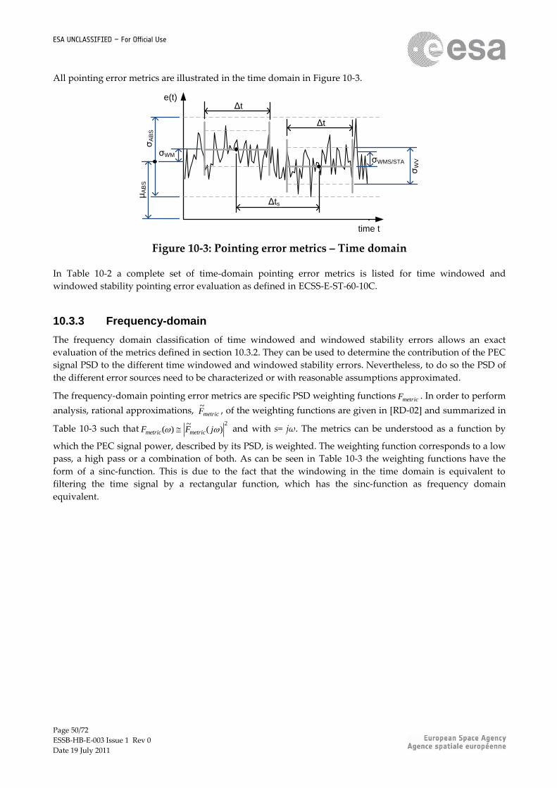
Page 50/72
ESSB-HB-E-003 Issue 1 Rev 0
Date 19 July 2011
ESA UNCLASSIFIED – For Official Use
All pointing error metrics are illustrated in the time domain in Figure 10-3.
e(t)
time t
Δt
σA
BS
µA
BS
σW
V
Δt
Δts
σWMS/STA
σWM
Figure 10-3: Pointing error metrics – Time domain
In Table 10-2 a complete set of time-domain pointing error metrics is listed for time windowed and
windowed stability pointing error evaluation as defined in ECSS-E-ST-60-10C.
10.3.3 Frequency-domain
The frequency domain classification of time windowed and windowed stability errors allows an exact
evaluation of the metrics defined in section 10.3.2. They can be used to determine the contribution of the PEC
signal PSD to the different time windowed and windowed stability errors. Nevertheless, to do so the PSD of
the different error sources need to be characterized or with reasonable assumptions approximated.
The frequency-domain pointing error metrics are specific PSD weighting functions metricF . In order to perform
analysis, rational approximations, metricF~
, of the weighting functions are given in [RD-02] and summarized in
Table 10-3 such that2
)(~
)( jFF metricmetric and with s= jω. The metrics can be understood as a function by
which the PEC signal power, described by its PSD, is weighted. The weighting function corresponds to a low
pass, a high pass or a combination of both. As can be seen in Table 10-3 the weighting functions have the
form of a sinc-function. This is due to the fact that the windowing in the time domain is equivalent to
filtering the time signal by a rectangular function, which has the sinc-function as frequency domain
equivalent.
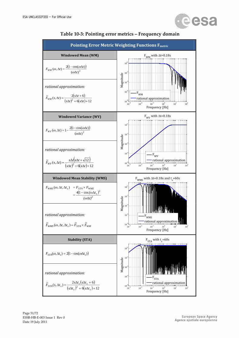
Page 51/72
ESSB-HB-E-003 Issue 1 Rev 0
Date 19 July 2011
ESA UNCLASSIFIED – For Official Use
Table 10-3: Pointing error metrics – Frequency domain
Pointing Error Metric Weighting Functions Fmetric
Windowed Mean (WM)
10-3
10-2
10-1
100
101
102
10-8
10-6
10-4
10-2
100
Frequency [Hz]
Mag
nit
ud
e
FWM
with t=0.18s
FWM
rational approximation
2)(
)cos(12),(
t
ttFWM
rational approximation:
126
62),(
~2
tsts
tstsFWM
Windowed Variance (WV)
10-3
10-2
10-1
100
101
102
10-8
10-6
10-4
10-2
100
Frequency [Hz]
Mag
nit
ud
e
FWV
with t=0.18s
FWV
rational approximation
2)(
)cos(121),(
t
ttFWV
rational approximation:
126
12),(
~2
tsts
tststsFWV
Windowed Mean Stability (WMS)
10-3
10-2
10-1
100
101
102
10-8
10-6
10-4
10-2
100
Frequency [Hz]
Mag
nit
ud
e
FWMS
with t=0.18s and ts=60s
FWMS
rational approximation
2
2cos14
),,(
t)(
t(ω
FFttF
s
WMESTAsWMS
rational approximation:
WMSTAsWMS FFttF~~
),,(~
Stability (STA)
10-3
10-2
10-1
100
101
102
10-8
10-6
10-4
10-2
100
Frequency [Hz]
Mag
nit
ud
e
FSTA
with ts=60s
FSTA
rational approximation
)cos(12),( ssSTA ttF
rational approximation:
126
62),(
~2
ss
sssSTA
tsts
tststsF
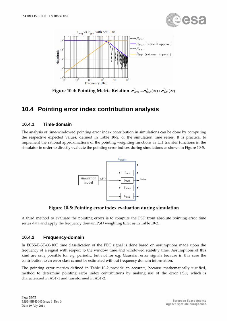
Page 52/72
ESSB-HB-E-003 Issue 1 Rev 0
Date 19 July 2011
ESA UNCLASSIFIED – For Official Use
Figure 10-4: Pointing Metric Relation )()( 222 tt WVWMABS
10.4 Pointing error index contribution analysis
10.4.1 Time-domain
The analysis of time-windowed pointing error index contribution in simulations can be done by computing
the respective expected values, defined in Table 10-2, of the simulation time series. It is practical to
implement the rational approximations of the pointing weighting functions as LTI transfer functions in the
simulator in order to directly evaluate the pointing error indices during simulations as shown in Figure 10-5.
FWM
FWMS
FWV
Fmetric
ec(t) εindex
FSTA
simulation model
Figure 10-5: Pointing error index evaluation during simulation
A third method to evaluate the pointing errors is to compute the PSD from absolute pointing error time
series data and apply the frequency domain PSD weighting filter as in Table 10-2.
10.4.2 Frequency-domain
In ECSS-E-ST-60-10C time classification of the PEC signal is done based on assumptions made upon the
frequency of a signal with respect to the window time and windowed stability time. Assumptions of this
kind are only possible for e.g. periodic, but not for e.g. Gaussian error signals because in this case the
contribution to an error class cannot be estimated without frequency domain information.
The pointing error metrics defined in Table 10-2 provide an accurate, because mathematically justified,
method to determine pointing error index contributions by making use of the error PSD, which is
characterized in AST-1 and transformed in AST-2.

Page 53/72
ESSB-HB-E-003 Issue 1 Rev 0
Date 19 July 2011
ESA UNCLASSIFIED – For Official Use
The frequency domain integrals of Table 10-2 can be evaluated by numerical integration or state-space
methods as shown in [RD-07].
10.5 Statistical interpretation of pointing error indices
During AST-3 it is important to express the statistical properties (i.e. mean and variance) with respect to the
statistical interpretation according to the guidelines provided in section 5.3.3 and 8.4. Before continuing with
AST-4, this is done for each pointing error index contributor (i.e. µindex or σindex) individually and analogous to
the PES statistical interpretation in AST-1.

Page 54/72
ESSB-HB-E-003 Issue 1 Rev 0
Date 19 July 2011
ESA UNCLASSIFIED – For Official Use
11 Pointing error evaluation: AST-4
11.1 Evaluation methods
As introduced in section 7.1, there are two methods for analysing pointing performance, the simplified
statistical method and the advanced statistical method. In the early development phases, when detailed
control design and hardware specifications are not yet available, the performance can be analysed by the
simplified statistical method. This method is based on the assumption that the central limit theorem applies.
As the design matures more information of the system (HW and SW) becomes available and the performance
can be evaluated by the advanced statistical method, which is more accurate because it considers the actual
shape of the PDF. Hence, pointing performance analysis is a combination of the simplified and advanced
statistical method changing throughout the development process.
As shown in Figure 11-1 the time-constant and time-random error contributors are first summed separately
and the probability with the applicable confidence level is computed. Thereafter, the total pointing error is
computed per error index from both intermediate results. These steps are described in this section 11 for the
simplified statistical approach. The advanced statistical approach is only briefly introduced.
Outputs
Inputsσindexμindex
B
compilation of total pointing error per index
eRPE/RKEeMPE/MKEeAPE/AKE ePDE/KDE ePRE/KRE
pBC
time-constant
time-random
σBC μBC
pN∗pN-1∗…∗p1pN∗pN-1∗…∗p1
εindex
Pc evaluation
pindex
ΣΣ Σ Σ
Pc evaluation
Figure 11-1: Pointing error evaluation
NOTE It is important that the statistical properties (i.e. variance and mean) are
expressed in terms of their statistical interpretation before compiling the
pointing error budget.

Page 55/72
ESSB-HB-E-003 Issue 1 Rev 0
Date 19 July 2011
ESA UNCLASSIFIED – For Official Use
11.2 Simplified method
11.2.1 Time-constant pointing error contributors per index
For time-constant errors, the summation and computation of the applicable probability is identical to the
time-random error case, as shown in Table 11-1.
Table 11-1: Time-constant pointing error summation
Time-Constant PEC: Summation and Level of Confidence Evaluation Pc evaluation summation
BBpnB
N
i
iB
1
222uccB
correlated
N
i
ic N
1
22 (*1)
or
2
1
2
N
i
ic (*2)
uncorrelated
N
i
iuc
1
22
B bias
2 variance
mean
N number of summands
cP
level of confidence:
pn
defines max. error complying
with
cP requirement of a Gaussian
distribution by pn
*1: general worst case upper bound summation (see Annex for derivation). *2: upper bound summation as in ECSS standard.

Page 56/72
ESSB-HB-E-003 Issue 1 Rev 0
Date 19 July 2011
ESA UNCLASSIFIED – For Official Use
11.2.2 Time-random pointing error contributors per index
In Table 11-2 the summation for the mean and variance of the different time-random pointing error
contributions are shown, where:
the means are summed linearly,
the uncorrelated variances are summed quadratic,
for the correlated variances upper bound estimation is used. There are two different computations of
the upper bound proposed in Table 11-2, which are derived in Annex E.
Note that the window time, windowed stability time and drift time dependencies are omitted in Table 11-2
to Table 11-1.
Table 11-2: Time-random PEC summation per index
TIME-RANDOM PEC: SUMMATION
statistics summation
sumindex_
N
i
i
1
2_ sumindex
group summation signal class groups
N
i
ic
N
i
iuc
1
2
1
2 )()(
correlated
N
i
ic N
1
22 (*1)
or
2
1
2
N
i
ic (*2)
uncorrelated
N
i
iuc
1
22
2 variance N number of summands
mean
*1: general worst case upper bound summation (see Annex for derivation).
*2: upper bound summation as in ECSS standard → suggested for periodic error summation.
The error index is then computed for the applicable confidence level. The method is shown in Table 11-3.
First the standard deviation is multiplied by np, where np is a positive scalar such that for a Gaussian
distribution the np confidence level encloses the probability Pc, as specified in the requirement. Then the
standard deviation is summed with the mean values.
NOTE Although the application of the central limit theorem is assumed, it is
recommended to check its applicability. In case of e.g. a dominant periodic error
the compilation of the budget should be adapted accordingly or the advanced
statistical method applied.

Page 57/72
ESSB-HB-E-003 Issue 1 Rev 0
Date 19 July 2011
ESA UNCLASSIFIED – For Official Use
Table 11-3: Level of confidence evaluation for time-windowed PEC per index
Time-Random PEC: Level of Confidence Evaluation
index Pc evaluation assuming applicability of
central limit theorem PC requirement
APE(∆tD,)/
AKE(∆tD)
indexDsumindexpindex tn )(,
cindex Pe )(Prob
MPE(∆t, ∆tD)/
MKE(∆t, ∆tD) indexDsumindexpindex ttn ),(,
RPE(∆t, ∆tD)/
RKE(∆t, ∆tD)
),(, Dsumindexpindex ttn
PDE(∆t, ∆ts, ∆tD)/
KDE(∆t, ∆ts, ∆tD)
),,(, Dssumindexpindex tttn
PRE(∆t, ∆ts)/
KRE(∆t, ∆ts)
),(, ssumindexpindex ttn
e pointing error
index
max. time-random error compliant with cP
index
mean of time-random error
Dt drift re-set time
cP
level of confidence
pn
defines error that complies with cP
requirement of a Gaussian
distribution by indexpn

Page 58/72
ESSB-HB-E-003 Issue 1 Rev 0
Date 19 July 2011
ESA UNCLASSIFIED – For Official Use
11.2.3 Compilation of total pointing error per index
Finally, the time-constant and time-random pointing errors are summed per APE, AKE, MPE and MKE
indices. On the other hand, the time-constant error does not contribute to the other pointing error indices. An
overview of the summation is shown in Table 11-4.
Table 11-4: Compilation of total pointing error per index
Total Pointing Error per Index index compilation
APE(∆tD)/
AKE(∆tD) )( Dindexindex tBe
MPE(∆t, ∆tD)/
MKE(∆t, ∆tD) ),( Dindexindex ttBe
RPE(∆t, ∆tD)/
RKE(∆t, ∆tD) ),( Dindexindex tte
PDE(∆t, ∆ts, ∆tD)/
KDE(∆t, ∆ts, ∆tD) ),,( Dsindexindex ttte
PRE(∆t, ∆ts)/
KRE(∆t, ∆ts) ),( sindexindex tte
indexe
max. error per index complying with cP
st stability time
t window time
Dt drift re-set time
11.3 Advanced method
This method corresponds to the so-called exact error combination method as defined in ECSS-E-ST-60-10C.
In order to apply the statistical method, each individual source is characterised in terms of probability
distribution function (e.g. uniform, Gaussian, bimodal distribution). Then time simulations are performed to
get a sufficient sample size representing the statistical behaviour of all error sources and of their potential
cross-correlation. This is often designated as ‚Monte Carlo simulations‛. For each run, pointing performance
is estimated and when all runs are performed, the results are presented in the form of a cumulative
histogram giving the expected performance as a function of the cumulated number of samples. Then, the
RMS (1) performance corresponds to the value which is not exceeded for 68.3% of the temporal samples.
The 2 performance corresponds to the value which is not exceeded for 95.5% of the temporal samples. The
worst case (3) performance corresponds to the value which is not exceeded for 99.7% of the temporal
samples.
Monte Carlo simulations and the related statistics are further elaborated in [RD-04].

Page 59/72
ESSB-HB-E-003 Issue 1 Rev 0
Date 19 July 2011
ESA UNCLASSIFIED – For Official Use
12 Conclusion
The ESA PEE Handbook provides an engineering step-by-step process ranging from the formulation of
system pointing error requirements, to systematic pointing error analysis, and eventually to the compilation
of pointing error budgets for compliance verification. The process is consistent with ECSS-E-ST-60-10CC
standard ECSS-E-ST-60-10C and complements it with additional elements like the PSD characterization and
the pointing error metrics. Moreover, it defines an interface for the unambiguous formulation of pointing
error requirements and provides guidelines, recommendations and examples for specific case of satellite
pointing error engineering. As the process has clearly separated steps with defined input and output data it
is quite generic and thus applicable to any mission type and design phase.
The ESA PEE Handbook together with the ECSS standard replaces the ‚old‛ ESA Pointing Error Handbook
[RD-08]. Furthermore, it is intended to complete the ESA PEE Handbook in the future by one or several
documents providing guidelines for the mapping process, i.e. the flow-down of application requirements
(e.g. from the ESA MRD) to pointing error requirements.

Page 60/72
ESSB-HB-E-003 Issue 1 Rev 0
Date 19 July 2011
ESA UNCLASSIFIED – For Official Use
Annex A Pointing scene
Considering a pointing scene, as shown in Figure A-1, the pointing error is described with respect to the
target plane. Translational pointing errors on the target plane are a result of rotational errors about the
pointing system axes. Hence rotational errors about pointing system x- and y-axis correspond to a
displacement error exθ and eyΦ on the target plane respectively. Rotational errors about the z-axis for any
point p on the target plane, however, produce rotational errors, that eventually can be mapped into
displacement errors along ex and ey or vice versa by:
cossin
sincos and th wi ΨlΨ RppepRe
p
p
y
x
y
x
e
e
[A-1]
where the directional boresight, line of sight (LOS) or half-cone error le is defined as:
y
x
e
ele with 22
yx ee le [A-2]
Hence the resulting pointing error is described by two translations and one rotation one the target plane or
by three rotations about the body axes of the pointing system.
ψ
Φ
θ
x
y
z
exey
Figure A-1: Pointing scene
x, y, z: pointing system axes with respective rotation angles θ, Φ, ψ.
ex, ey: LOS error coordinates on target plane .
NOTE Rotational errors with a Gaussian distribution about the x- and y-axis result in a
Rayleigh distribution (see Table 5-1) about the LOS, cf. ECSS-E-ST-60-10C.

Page 61/72
ESSB-HB-E-003 Issue 1 Rev 0
Date 19 July 2011
ESA UNCLASSIFIED – For Official Use
Annex B Pointing error description using different
statistical interpretations
B.1 Satellite pointing example
In this Annex B a simplified satellite pointing example is illustrated to support the introduced methodology
in this handbook. The satellite system is shown schematically in Figure B-1.
satellite structure
satellite
+e
attitude control
+
attitudeestimatior
ec1
eSTRUC ec2
eAE
es2
es3
es5
es1
es4
es6
eAC ec3
Figure B-1: Satellite pointing example
The satellite system is affected by the PES listed in Table B-1.
Table B-1: PES in satellite pointing example
PES Type
es1 Payload-star tracker misalignments
es2 µVibrations (outside of control bandwidth)
es3 Reaction wheel errors
es4 External disturbances
es5 Star tracker errors
es6 Gyro errors
In Table B-2 three exemplary PES are taken from the satellite pointing example in Figure B-1 and Table B-1.
They are described in line with the analysis method introduced in section 7. Two different misalignment
errors are taken into account to show the difference between an ensemble-random PES and the more
complex case of a time- and ensemble-random PES. For the AOCS gyro-stellar estimator noise two different

Page 62/72
ESSB-HB-E-003 Issue 1 Rev 0
Date 19 July 2011
ESA UNCLASSIFIED – For Official Use
cases are treated, in one the PES is time-random only and in the other one the PES is time-random and
ensemble-random.
In AST-1 to AST-3 the pointing errors (PES, PEC and error index contributor) can be categorized as in Table
B-3. Note that the attitude estimator PEC, which is a PES for the attitude control, is the transformation of the
gyro and star tracker PES by the attitude estimator. Further details on Star Tracker PES are provided in
section 5.5 of ECSS-E-ST-60-20C Rev 1.
Table B-2: PES examples
Pointing Error Sources or Contributors – PES or PEC
Payload-STR
misalignment
Time-constant misalignment errors (STR internal, Payload internal, structure) with
uniformly distributed error values among an ensemble of satellites (before in-orbit
calibration)
Payload-STR thermo-
elastic distortion
Payload-STR thermo-elastic misalignment errors with sinusoidal (assumed) variation of
different periods (cross-correlated or none cross-correlated). In addition, the
amplitudes have uniformly distributed uncertainty errors due to seasonal effects.
AOCS gyro-stellar
estimator bias
Attitude knowledge bias error originating from star tracker pixel and FOV spatial errors.
In a first approach, the bias error can be assigned a uniform distribution because
different stellar configurations are assumed to have equal probability.
AOCS gyro-stellar
estimator noise
Attitude knowledge Gaussian noise originating from gyro and star tracker temporal
noise. In a first approach the RMS noise power is time-constant.
AOCS gyro-stellar
estimator noise
-attitude dependent
Attitude knowledge Gaussian noise originating from sensor measurement noise. The
RMS noise power has a uniformly distributed uncertainty error due to different
operational conditions.
Table B-3: Categorization of pointing errors examples
PES/PEC temporal
behavior
signal
class
time-
random
variable
description ensemble-random
variable
Payload-STR misalignment
time-constant
bias none random variable misalignment bias
Payload-STR thermo-elastic distortion
time-random
periodic misalignment magnitude
zero-mean stationary random process with bi-modal PDF
uniformly distributed amplitude A of periodic variation due to different operational conditions
AOCS gyro-stellar estimator bias
time-random
bias(t) bias magnitude
random variable none
AOCS gyro-stellar estimator noise
time-random
random noise error magnitude
zero-mean stationary random process with Gaussian PDF
none
AOCS gyro-stellar estimator noise- attitude dependent
time-random
random noise error magnitude
zero-mean stationary random process with Gaussian PDF
uniformly distributed noise RMS value σ due to different operational conditions

Page 63/72
ESSB-HB-E-003 Issue 1 Rev 0
Date 19 July 2011
ESA UNCLASSIFIED – For Official Use
B.2 Time-constant description
The time constant pointing error (PES and PEC) are described in Table B-4 according to their categorization
and signal class by means of the respective statistical properties and their PDF.
Table B-4: Time-constant pointing error description
time-constant PES/PEC
statistical interpret.
random variable description
pSC(e) μSC(e) σSC(e)
Payload-STR misalignment
ensemble Sigma value of uniformly distributed misalignment error.
U(0, emax ) 0 σU
temporal Maximum misalignment error.
δ(emax) C 0
mixed Same as ‘ensemble’ because temporal behavior is constant.
U(0, emax ) 0 σU
The mixed (or ensemble) interpretation allows a realistic statistical approach in the quadratic summation of
constant biases in the last AST-4 step, while the temporal approach forces an arithmetic summation of all
worst case elementary biases.
B.3 Time-random pointing error description by a random variable
The time-random pointing error (PES and PEC) are described in Table B-5 according to their categorization
and signal class by means of the respective statistical properties and their PDF.
Table B-5: Time-random pointing error description by random variable theory
time-random PES/PEC
statistical interpret.
random variable description
pSR(e) μSR σSR
AOCS gyro-stellar estimator bias
ensemble Worst case bias error. δ(emax) emax 0
temporal Sigma value of uniformly distributed bias error.
U(0, emax) 0 σU
mixed Same as ‘temporal’ because ensemble behavior is constant.
U(0, emax) 0 σU
B.4 Time-random pointing error description by a random process
The time-random pointing error (PES and PEC) are described in Table B-6 according to their categorization
and signal class by means of the respective statistical properties and their PDF.

Page 64/72
ESSB-HB-E-003 Issue 1 Rev 0
Date 19 July 2011
ESA UNCLASSIFIED – For Official Use
Table B-6: Time-random pointing error description by random process theory
time-random PES/PEC
statistical interpret.
random process description
pSRP(e) µSRP σSRP
AOCS gyro-stellar estimator noise
ensemble Maximum noise magnitude (Gaussian noise is unbounded => 3 sigma value).
δ(emax) emax=3σG
emax 0
temporal Sigma (or zero-mean RMS) value of Gaussian noise process.
G(0,σG) 0 σG
mixed Same as ‘temporal’ because ensemble behavior is constant.
G(0,σG) 0 σG
B.5 Time-random and ensemble-random pointing error description by a random process
The time-random pointing error (PES and PEC) are described in Table B-7 according to their categorization
and signal class by means of the respective statistical properties and their PDF.
Table B-7: Time- and ensemble-random PES description by random process theory
time-random PES/PEC
statistical interpret.
random process description
pSRP(e) σSRP
Payload-STR thermo-elastic distortion
ensemble Sigma value of uniformly distributed misalignment variation amplitude.
U(0, emax) emax =Amax
σU
temporal
Sigma (or zero-mean RMS) value of periodic misalignment variation with maximum amplitude.
BM(emax) emax =Amax
σBM
mixed
Sigma value of uniformly distributed sigma (or zero-mean RMS) noise value of uniformly distributed periodic misalignment variation with amplitude A.
∫ p(e|A)p(A)de = ∫ BM(A)U(0, Amax)de
σ(A)
AOCS gyro-stellar estimator noise - attitude dependent
ensemble
Sigma value of uniformly distributed maximum noise magnitude (Gaussian noise is unbounded => 3 sigma value).
U(0, emax) emax =3σG, max
σU
temporal Sigma (or zero-mean RMS) value of Gaussian noise process with maximum sigma.
G(0, σG,max) σG
mixed
Sigma value of Gaussian ensemble-random and time-random noise process if stationary.
G(0, σG) σG
Page 65/72
ESSB-HB-E-003 Issue 1 Rev 0
Date 19 July 2011
ESA UNCLASSIFIED – For Official Use
Annex C Signal and system norms for pointing error
analysis
C.1 Overview
Signal norms are convenient for measuring the size of a pointing error signal entering and leaving a system.
On the other hand system norms are convenient to determine the gain for such a system transformation of
pointing signal norms. Considering e.g. the AOCS of a satellite, PES entering and PEC leaving the system can
be quantified in terms of signal norms to determine the AOCS closed loop pointing error performance. In
this sense several norms exist to measure the size of a pointing error signal. The selection of the appropriate
norm depends on the nature of the signal and its requirement.
It is important to mention that norms considered in this document have seminorm properties as defined in
[RD-05].
C.2 Signal norms
In the following some important signal norms are introduced:
L1-norm:
dttee
0
1)(: [C-1]
The L1-norm defines the absolute integral error of a signal. It is useful to measure the total amount of
consumables in a system, e.g. propellant consumption of a satellite.
L2-norm:
2/1
0
2
2)(:
dttee [C-2]
The L2-norm is a measure of total signal energy. It is appropriate to e.g. measure the size of a transient signal
occurring during satellite re-orientation.
Lp-norm:
p with dttee
p
p
p1 )(:
/1
0
[C-3]
The Lp-norm is the general formulation of the L1- and L2-norm.

Page 66/72
ESSB-HB-E-003 Issue 1 Rev 0
Date 19 July 2011
ESA UNCLASSIFIED – For Official Use
L∞-norm:
)(sup:0
teet
[C-4]
The L∞-norm corresponds to the absolute peak value of a signal. It can be used to limit the absolute value of a
signal, e.g. a satellite tracking error.
RMS-norm:
2/1
2)(2
1lim:
dtteT
e
T
TTrms
[C-5]
The RMS-norm squared is a measure of the steady-state power of a signal. Note that even though a signal
has a small RMS-norm it might be large for some short time periods.
RMS-norm for stationary random processes:
time-domain: 2/12 ])([: teEerms
frequency-domain:
2/1
)(2
1:
dSe eerms
[C-6]
with E*…+ being the expected value and See(ω) the double-sided PSD in [unit2/rad s-1]. The general definition
of the RMS-norm in Eq. [C-5] is equal to the RMS-norm of stationary random processes in Eq. [C-6] if the
stationary random process is ergodic. The RMS-norm is a suitable measure of e.g. the expected PEC if the
PES is a random stationary noise process.
C.3 System norms
12.1.1.1.1 Induced System Norms
The induced system norm corresponds to the maximum gain of a system and is specified as:
ps
ps
eps
pc
eindp e
He
e
ejH
psps 00,
supsup:)(
[C-7]
The induced system norm measures the size of the output PEC, ec(t), for the worst case input PES, es(t). Thus
it allows analysing the system transformation of pointing error signals as required in section 9. This is
possible if the pointing error signal is quantified with the above signal norms and the system has a linear,
time-invariant, causal, and finite-dimensional transfer function, H(jω).
In the following some important induced system norms are introduced:
L2-norm induced:
)sup)
supsup:)()(
0
2
2
02
2
0,2
H(jω:H(jωwith
e
He
e
ejHjH
ω
s
s
es
c
eind
psps
[C-8]
The induced L2-norm corresponds to the H∞-norm and represents the energy-gain for the PES system
transfer.
Page 67/72
ESSB-HB-E-003 Issue 1 Rev 0
Date 19 July 2011
ESA UNCLASSIFIED – For Official Use
L∞-norm induced:
)()(
supsup:)()(
0
1
001,
dtththwith
e
He
e
ethjH
s
s
es
c
eind
ss
[C-9]
The induced L∞-norm corresponds to the L1-norm of the impulse response, h(t)=δ(t), of the transfer function
H(jω). It represents the system gain for the PES signal peak value transformation.
RMS-norm induced:
jHjHwith
e
He
e
ejHjH
rmss
rmss
ermss
rmsc
eindrms
rmssrmss
)(sup:)(
supsup:)()(
0
00,
[C-10]
The induced RMS-norm corresponds to the H∞-norm and represents the RMS-gain for the PES system
transfer.
H2-norm:
In case the PES is a random stationary noise process with a certain PSD See(ω) the RMS-norm of the output
PEC is:
2/1
2)()(
2
1
dSjHe eermsc [C-11]
If See(ω)=1, the RMS-norm of ec(t) corresponds to system H2-norm:
2/1
2
2)(
2
1:)(
djHjH [C-12]
The H2-norm is a measure of system gain with white noise input. It is not an induced system norm, but it is
relevant in many practical cases where a PES can be approximated as white noise. Furthermore, by
Parseval’s theorem the H2-norm of a system corresponds to the L2-norm of the system’s impulse response
signal, h(t):
).()( , )(2
1)(
2/1
2
2/1
0
2
2thtewithedjHdtthe crmscc
[C-13]
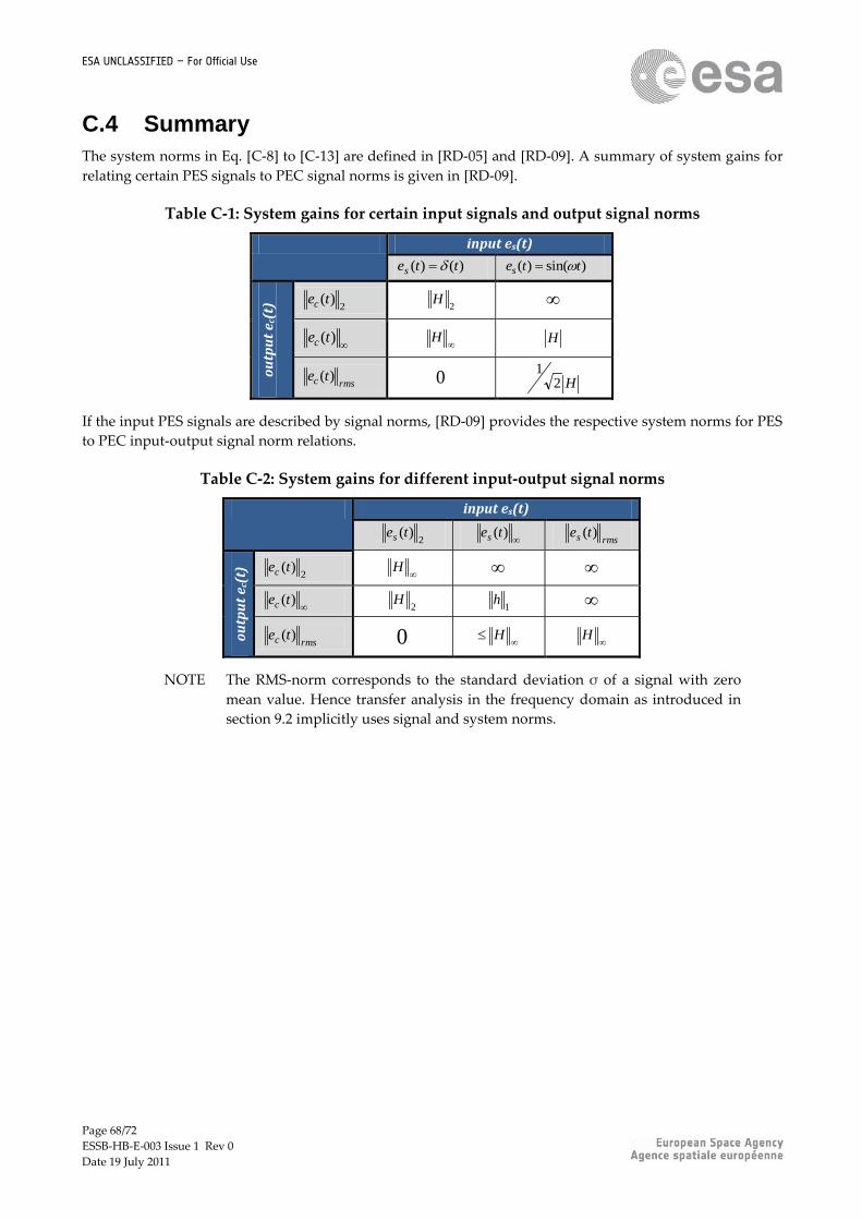
Page 68/72
ESSB-HB-E-003 Issue 1 Rev 0
Date 19 July 2011
ESA UNCLASSIFIED – For Official Use
C.4 Summary
The system norms in Eq. [C-8] to [C-13] are defined in [RD-05] and [RD-09]. A summary of system gains for
relating certain PES signals to PEC signal norms is given in [RD-09].
Table C-1: System gains for certain input signals and output signal norms
input es(t)
)()( ttes )sin()( ttes o
utp
ut
e c(t
) 2)(tec
2H
)(tec
H H
rmsc te )( 0 H21
If the input PES signals are described by signal norms, [RD-09] provides the respective system norms for PES
to PEC input-output signal norm relations.
Table C-2: System gains for different input-output signal norms
input es(t)
2)(tes
)(tes
rmss te )(
ou
tpu
t e c
(t)
2)(tec
H
)(tec
2H
1h
rmsc te )( 0 H
H
NOTE The RMS-norm corresponds to the standard deviation σ of a signal with zero
mean value. Hence transfer analysis in the frequency domain as introduced in
section 9.2 implicitly uses signal and system norms.

Page 69/72
ESSB-HB-E-003 Issue 1 Rev 0
Date 19 July 2011
ESA UNCLASSIFIED – For Official Use
Annex D Notes on pointing error metrics
D.1 Windowed mean stability (WMS) metric
The windowed mean stability (WMS) metric for determining the pointing error index PDE, PRE, KDE, KRE
is a combination of the windowed mean (WM) metric and the stability (STA) metric. This becomes obvious
by looking at the PSD in Figure D-1 of the pointing error weighted by the metric weighting filter, FSTA and
FWME.
Figure D-1: Pointing error metric weighting function relation: FWMS = FWM x FSTA
D.2 Relation Allan Variance and WMS metric (PDE/PRE)
The Allan Variance, commonly used to describe performance errors of gyros and frequency stability errors in
clocks, is a specific case of the windowed stability metric described in Table 10-2. Considering the PSD
weighting filter of Table 10-3 and setting Δts=Δt we get:
2
4
2
2/
)2/(sin
cos12cos12
)()()(
)t(
t
t)(
t)(-t)(-
tFtFtF WMSTAWMS
[D-1]
Taking this weighting function and inserting it in the WMS weighting function results in the Allan Variance:

Page 70/72
ESSB-HB-E-003 Issue 1 Rev 0
Date 19 July 2011
ESA UNCLASSIFIED – For Official Use
d
)t(
tSt eeWMS 2
4
0
2
2/
)2/(sin2
2
1)(
[D-2]
D.3 Transformation from Allan Variance to PSD
This transformation is possible, but with the consequence of major loss of accuracy. This is because the
process of Allan Variance needs to be split into sections of common inclination. It can be decided between
different inclinations (noise types), that have different mathematical formulations to transform the Allan
Variance to a PSD. The approach can be found in detail in [RD-010].

Page 71/72
ESSB-HB-E-003 Issue 1 Rev 0
Date 19 July 2011
ESA UNCLASSIFIED – For Official Use
Annex E Notes on summation rules
E.1 Overview
Analyzing pointing error contributors also requires the analysis of their cross-correlation when they are
effective at the same time. However, a cross-correlation analysis of pointing error contributors might not
always be possible. In the following rules are derived for the summation of pointing error contributors. The
errors are considered to be zero-mean errors (eA, eB, eC), that can either be described as random process or
random variable.
E.2 Sum of mean square values for cross-correlated errors
In this section E.2 a formula is derived for summing errors that have an unknown degree of cross-correlation.
This is done by considering the worst case cross-correlation among errors such that an upper bound
summation is performed.
The variance of the sum of errors is described by the expected value:
)()()()(
)]([)]()([)]()([
)]()([)]([)]()([
)]()([)]()([)]([)]([
2
2
222
tetetetewith
teEteteEteteE
teteEteEteteE
teteEteteEteEteE
CBA
CBCAC
CBBAB
CABAAe
[E-1]
If the degree of cross-correlation is unknown, the following inequality can be applied:
)]([)]([2
1)]()([
0)]([)]()([2)]([
teEteEteteE
teEteteEteE
yxyx
yyxx
[E-2]
thus it follows that:
22222222 333)]([3)]([3)]([3 )]([ CBA eeeCBAe teEteEteEteE [E-3]
In the general case that means:
N
1i
2
222
222
21
22
N
...
)]([...)]([)]([ )]([
21
i
eee
Ne
NNNN
teENteENteENteE
[E-4]

Page 72/72
ESSB-HB-E-003 Issue 1 Rev 0
Date 19 July 2011
ESA UNCLASSIFIED – For Official Use
E.3 Sum of mean square values for none cross-correlated errors
In this section E.3 a formula is derived for summing errors that have no cross-correlation.
If the errors are not correlated, then the following relation applies:
)()()()(
)]([)]([)]([)]([ 22222
tetetetewith
teEteEteEteE
CBA
CBAe
[E-5]
meaning that the cross-correlation terms vanish because they are zero. Thus the general summation rule is:
N
1i
2
222
222
21
22
...
)]([...)]([)]([ )]([
21
i
eee
Ne
N
teEteEteEteE
[E-6]
![An Error Model for Pointing Based on Fitts’ Law · DERIVATION OF AN ERROR MODEL FOR POINTING Formulated for one dimension, Fitts’ law [8] predicts the movement time MT to acquire](https://static.fdocuments.net/doc/165x107/5e1edcaeaa9d7041406d2f54/an-error-model-for-pointing-based-on-fittsa-law-derivation-of-an-error-model-for.jpg)