ERS186: Environmental Remote Sensing€¦ · with the various signatures and assigned to the class...
54
Transcript of ERS186: Environmental Remote Sensing€¦ · with the various signatures and assigned to the class...
MERMS 12 - L4
Classifying
Stuart Green
Earthobservationwordpresscom
StuartGreenTeagascie
Classifying
bull Replacing the digital numbers in each pixel (that tell us
the average spectral properties of everything in the pixel)
with a single number-a code that might represent the
majority landusecover in the pixel a biophysical
property in the pixel (amount of biomass) or a relative
value for a Landover (percentage of pixel that is
forestry)
bull httpslandmappingwordpresscom
MERMS 12 - L4
Main Routes to creating a Thematic
Landcover Map
bull Manual Digitisation and Interpretation
bull Photomorphic Labelling
bull Unsupervised Classification
bull Supervised Classification
ndash Maxiumum Likelihood
ndash Random Forest
ndash Support Vector Machine
bull Object Orientated
bull Hybrid Approaches
Supervised classification is much more accurate for mapping classes but depends
heavily on the cognition and skills of the image specialist The strategy is simple
specialist must recognize conventional classes from prior knowledge
Training sites are areas representing each known land cover category that appear fairly
homogeneous on the image (as determined by similarity in tone or color within shapes
delineating the category) Specialists locate and circumscribe them with polygonal
boundaries drawn (using the computer mouse) on the image display For each class
thus outlined mean values and variances of the DNs for each band used to classify
them are calculated from all the pixels enclosed in the site
When DNs are plotted as a function of the band sequence (increasing with wavelength)
the result is a spectral signature or spectral response curve for that class
Classification now proceeds by statistical processing in which every pixel is compared
with the various signatures and assigned to the class whose signature comes closest A
few pixels in a scene do not match and remain unclassified because these may belong
to a class not recognized or defined)
Supervised Classification
Pick themes you want to map These have to be ldquomappablerdquo Ie within the capabilities of being detected with the sensorimage you are using
So they have to be greater than the resolution of your image (in our case 25m)
They have to be observable (for optical systems this means ldquovisiblerdquo on the surface)
Identify and delinate training areas
bull These have to be good homogenoues
areas that truly represent the cover type
you are interested in Most cover types will
have a number of traing areas to fully
define the range of values present in the
image
BAD
BAD
Chose the algotithm that will
allocate pixels into your classess
Some Types of Classifiers
bull Non-parametric
ndash Parallelepiped classifier (BOX or PPD)
ndash Minimum-distance-to-means (MDM)
ndash Expert Systems
Parametric
ndash Maximum likelihood (ML)
ndash Neural networks
A parametric signature is based on statistical parameters (eg mean and covariance
matrix) of the pixels that are in the training sample or cluster Supervised and
unsupervised training can generate parametric signatures A set of parametric
signatures can be used to train a statistically-based classifier to define the classes
A nonparametric signature is not based on statistics but on discrete objects (polygons or
rectangles) in a feature space image These feature space objects are used to define
the boundaries for the classes
A nonparametric classifier uses a set of nonparametric signatures to assign pixels to a
class based on their location either inside or outside the
area in the feature space image Supervised training is used to generate nonparametric
signatures (Kloer 1994)
Parallelepiped
bull The minimum and maximum DNs for each class are determined and are used as thresholds for classifying the image
bull Benefits simple to train and use computationally fast
bull Drawbacks pixels in the gaps between the parallelepipes can not be classified pixels in the region of overlapping parallelepipes can not be classified
Feature Space tools enable you to interactively define feature
space objects in the feature space image(s) A feature space image is simply a
graph of the data file values of one band of data against the values of another
band (often called a scatterplot)
Parallelepiped
Minimum-Distance-to-Means
Candidate Pixel
to be classified
Class 1 means
Class 2 means
Band 2
Band 1
D1
D2
D1 lt D2 so the pixel is classified
as Class 1
Maximum Likelihood
Machine Learning
Random Forest and Support Vector Machines
bull These techniques whilst easily applied
are beyond the technical scope of this
short course
bull However we have shown the RF is the
best suited method for Irish mapping
MERMS 12 - L4
You can try these methods
using SAGA a free GIS that is
also compatible with ArcGIS
MERMS 12 - L4
httpwwwsaga-gisorgenindexhtml
From Pixels to Objects
Previously we have looked at classification based
only on the spectral characteristics of pixels one
by one But the information in an image isnt
encoded in pixels but objects- things we
recognise
Objects are things on the
Ground
bull Object Orientated Classifcation attempts
to bring to gether many of the aspects of
image interpreatation that we looked at
early in the course on manual
interpretation of imagery- like shadow
texture context etc
bull But do so in an automated fashion so the
computer can create the outptut
Objects
bull We can have a-priori defined objects ndash
cadastral maps for example (Prime 2 in
the Irish context)
bull Or we can create objects from the image
using segmentation
Unclosed areas
bull What does landcover mean in these
areas
bull How best to record extent and change
bull Classifications havent been finalised- but
will be guided by Helm and Eagle
Internationally Fossit locally and at all
times with practicallity in mind
Segmentation
bull Essentially the segmentation algorithm examines how like its neighbours a pixel is- if pixels are alike they are grouped into objects
bull We can use colour of texture or the shape of the object to help us segment an image- most popular software for soing this is e-cognition
bull Its very simalr to the human interpreation approach of mapping ldquophotomorphic regionsrdquo and has been developed out of machine vision reserach
These segments become objects
bull WE can then xclassify the object suing any of
the classifcation we have looked at
bull Unsupervised
bull Supervised
bull Rule based or descsion tree
bull We can also include non-spectral data eg the
size of the object or its shape the variation of
pixels within an object (texture)
Scale15
Color02
Scale15
Color035
Scale50
Color02
Scale15
Color05
bull 22 OBIA Strengths
bull 1048707 Partitioning an image into objects is akin to the way
bull humans conceptually organize the landscape to
bull comprehend it
bull 1048707 Using image-objects as basic units reduces computational
bull classifier and at the sametime enables the user to take advantage of more complex
bull techniques (eg non-parametric)
bull 1048707 Image-objects exhibit useful features that single pixels lack
bull 1048707 Image-objects can be more readily integrated in vector
bull GIS
bull 23 OBIA Weaknesses
bull 1048707 There are numerous challenges involved in processing
bull very large datasets Even if OBIA is more efficient than
bull pixel-based approaches segmenting a multispectral image
bull of several tens of mega-pixels is a formidable task
bull 1048707 Segmentation is an ill-posed problem in the sense it has
bull no unique solution
bull 1048707 There exists a poor understanding of scale and hierarchical
bull relations among objects derived at different resolutions
bull Do segments at coarse resolutions really lsquoemergersquo or
bull lsquoevolversquo from the ones at finer resolutions Should
bull boundaries perfectly overlap (coincide) through scale
bull Operationally itrsquos very appealing but what is the
bull ecological basis for this
httpdesktoparcgiscomenarcmap103toolsspatial-
analyst-toolboxunderstanding-segmentation-and-
classificationhtm
bull The Classify Raster tool performs an image classification as
specified by the Esri classifier definition file Inputs to the tool include the image to be classified the optional segmented raster (such as another raster dataset or a layer such as a DEM) and a classifier definition file to generate the classified raster dataset Note that the Classify Raster tool contains all the supported classifiers The proper classifier is utilized depending on the properties and information contained in the classifier definition file So the classifier definition file generated by the Train ISO Cluster Classifier Train Maximum Likelihood Classifier or Train Support Vector Machine Classifier will activate the corresponding classifier when you run Classify Raster
Purposes of Field Data
bull To verify evaluate or assess the results of
remote sensing investigations (accuracy
assessment)
bull Provide data to geographically correct imagery
bull Provide information used to model the spectral
behaviour of landscape features (plants soils or
waterbodies)
Field data includes least three
kinds of information
bull Attributes or measurements that describe
ground conditions at a specific place
bull Observations must be linked to locational
information so the attributes can be
correctly matched to corresponding points
in image data
bull Observations must also be described with
respect to time and date
Geographic Sampling
bull Observation signifies the selection of a specific cell or pixel
bull Sample is used here to designate a set of observations that will be used in an error matrix
bull Three separate decisions must be made when sampling maps or spatial patterns
bull (1) Number of observations to be used
bull (2) Sampling pattern to position observations within an image
bull (3) Spacing of observations
Numbers of Observations
bull Number of observations determines
ndash the confidence interval of an estimate of the
accuracy of a classification A large sample size
decreases the width of the confidence interval of
our estimate of a statistic
bull For most purposes it is necessary to have
some minimum number of observations
assigned to each class
Sampling Pattern
The Simple Random Sampling Pattern
bull The choice of any specific location as the site for an observation is independent of the selection of any other location as an observation
bull All portions of a region are equally subject to selection for the sample thereby yielding data that accurately represent the area examined and satisfying one of the fundamental requirements of inferential statistics
The Stratified Random Pattern
bull Assigns observations to sub-regions of the image to ensure that the sampling effort is distributed in a rational manner A stratified sampling effort might plan to assign specific number of observations to each category on a map to be evaluated This procedure would ensure that every category would be sampled
bull
Systematic Patterns
This pattern positions
samples such that
observations are taken
at equal intervals
according to a specific
strategy Systematic
sampling is useful if it is
necessary to ensure
that all regions within a
study area are
represented
Systematic Stratified Unaligned Patterns
bull This pattern combines features of both systematic and stratified samples while simultaneously preserving an element of randomness
bull The entire study area is divided into uniform cells
bull The grid cells introduce a systematic component to the sample and form the basis for the stratification one observation is placed in each cell
bull An element of randomness is contributed by the method of placing observations within each cell
Cluster Sampling
bull Cluster Sampling selects points within a study area and uses each point as a centre to determine locations of additional ldquosatelliterdquo observations placed nearby so that the overall distribution of observations forms a clustered pattern
Cluster sampling may be efficient with respect to
time and finance If the pattern to be sampled is
known beforehand it may provide reasonably
accurate results
LOCATIONAL INFORMATION
bull Identification of Ground Control Points (GCPs) which allow analysts to resample image data to provide accurate planimetric location and correctly match image detail to maps and other images
bull Often we would use points of a map (sayu road intersections) to geometrically correct an Image but in some cases we have to identify a feature on the image and go out and survey that point on the ground in order to get accutare geographci correction
bull Additional information from
bull httpeuropaeuintcommspaceindex_enhtml
bull httpeuropaeuintcommdgsenergy_transportgalileo
bull httpwwwgalileojucom
bull httpwwwesaintesaNAgalileohtml
bull httpwwwosiiewp-contentuploads201507Survey-
Ireland-2004-GPS-Network-RTK-Solution-for-
Irelandpdfext=pdf
Accuracy Assessment
We may define accuracy in a working sense as the degree of correspondence between
observation and reality We usually judge accuracy against existing maps large scale aerial photos
or field checks We can pose two fundamental questions about accuracy
Is each category in a classification really present at the points specified on a map
Are the boundaries separating categories valid as located
Various types of errors diminish the accuracy of feature identification and category distribution We
make most of the errors either in measuring or in sampling When quantifying accuracy we must
adjust for the lack of equivalence and totality if possible Another often overlooked point about
maps as reference standards concerns their intrinsic or absolute accuracy Maps require an
independent frame of reference to establish their own validity
As a general rule the level of accuracy obtainable in a remote sensing classification depends on
diverse factors such as the suitability of training sites the size shape distribution and frequency
of occurrence of individual areas assigned to each class the sensor performance and resolution
and the methods involved in classifying (visual photointerpreting versus computer-aided statistical
classifying) and others
In practice we may test classification accuracy in four ways
1) field checks at selected points (usually non-rigorous and subjective) chosen either at
random or along a grid
2) estimate (non-rigorous) the agreement of the theme or class identity between a class
map and reference maps determined usually by overlaying one on the other(s)
3) statistical analysis (rigorous) of numerical data developed in sampling measuring and
processing data using tests such as root mean square standard error analysis of
variance correlation coefficients linear or multiple regression analysis and Chi-square
testing
4) confusion matrix calculations (rigorous)
With the class identities in the photo as the standard we arranged the number of pixels
correctly assigned to each class and those misassigned to other classes in the confusion
matrix listing errors of commission omission and overall accuracies
The producers accuracy relates to the probability that a reference sample (photo-
interpreted land cover class in this project) will be correctly mapped and measures
the errors of omission (1 - producers accuracy)
In contrast the users accuracy indicates the probability that a sample from land
cover map actually matches what it is from the reference data (photo-interpreted
land cover class in this project) and measures the error of commission (1- uses
accuracy)
Errors of commission An error of commission results when a pixel is committed to an
incorrect class
Errors of omission An error of omission results when a pixel is incorrectly classified
into another category The pixel is omitted from its correct class
urban grass natural water forestry map
urban 12 5 1 6 7 31
grass 1 34 7 2 44
natural 2 9 23 6 40
water 14 2 16
forestry 4 20 24
ground
15 48 31 24 37 155
Urban Ommission (31-12)31= 61
So Producers accuracy is 39
Urban Comission (15-12)15= 25
So users accuracy is 75
Total mapp accuray is (12+34+23+14+20)155 = 66

MERMS 12 - L4
Main Routes to creating a Thematic
Landcover Map
bull Manual Digitisation and Interpretation
bull Photomorphic Labelling
bull Unsupervised Classification
bull Supervised Classification
ndash Maxiumum Likelihood
ndash Random Forest
ndash Support Vector Machine
bull Object Orientated
bull Hybrid Approaches
Supervised classification is much more accurate for mapping classes but depends
heavily on the cognition and skills of the image specialist The strategy is simple
specialist must recognize conventional classes from prior knowledge
Training sites are areas representing each known land cover category that appear fairly
homogeneous on the image (as determined by similarity in tone or color within shapes
delineating the category) Specialists locate and circumscribe them with polygonal
boundaries drawn (using the computer mouse) on the image display For each class
thus outlined mean values and variances of the DNs for each band used to classify
them are calculated from all the pixels enclosed in the site
When DNs are plotted as a function of the band sequence (increasing with wavelength)
the result is a spectral signature or spectral response curve for that class
Classification now proceeds by statistical processing in which every pixel is compared
with the various signatures and assigned to the class whose signature comes closest A
few pixels in a scene do not match and remain unclassified because these may belong
to a class not recognized or defined)
Supervised Classification
Pick themes you want to map These have to be ldquomappablerdquo Ie within the capabilities of being detected with the sensorimage you are using
So they have to be greater than the resolution of your image (in our case 25m)
They have to be observable (for optical systems this means ldquovisiblerdquo on the surface)
Identify and delinate training areas
bull These have to be good homogenoues
areas that truly represent the cover type
you are interested in Most cover types will
have a number of traing areas to fully
define the range of values present in the
image
BAD
BAD
Chose the algotithm that will
allocate pixels into your classess
Some Types of Classifiers
bull Non-parametric
ndash Parallelepiped classifier (BOX or PPD)
ndash Minimum-distance-to-means (MDM)
ndash Expert Systems
Parametric
ndash Maximum likelihood (ML)
ndash Neural networks
A parametric signature is based on statistical parameters (eg mean and covariance
matrix) of the pixels that are in the training sample or cluster Supervised and
unsupervised training can generate parametric signatures A set of parametric
signatures can be used to train a statistically-based classifier to define the classes
A nonparametric signature is not based on statistics but on discrete objects (polygons or
rectangles) in a feature space image These feature space objects are used to define
the boundaries for the classes
A nonparametric classifier uses a set of nonparametric signatures to assign pixels to a
class based on their location either inside or outside the
area in the feature space image Supervised training is used to generate nonparametric
signatures (Kloer 1994)
Parallelepiped
bull The minimum and maximum DNs for each class are determined and are used as thresholds for classifying the image
bull Benefits simple to train and use computationally fast
bull Drawbacks pixels in the gaps between the parallelepipes can not be classified pixels in the region of overlapping parallelepipes can not be classified
Feature Space tools enable you to interactively define feature
space objects in the feature space image(s) A feature space image is simply a
graph of the data file values of one band of data against the values of another
band (often called a scatterplot)
Parallelepiped
Minimum-Distance-to-Means
Candidate Pixel
to be classified
Class 1 means
Class 2 means
Band 2
Band 1
D1
D2
D1 lt D2 so the pixel is classified
as Class 1
Maximum Likelihood
Machine Learning
Random Forest and Support Vector Machines
bull These techniques whilst easily applied
are beyond the technical scope of this
short course
bull However we have shown the RF is the
best suited method for Irish mapping
MERMS 12 - L4
You can try these methods
using SAGA a free GIS that is
also compatible with ArcGIS
MERMS 12 - L4
httpwwwsaga-gisorgenindexhtml
From Pixels to Objects
Previously we have looked at classification based
only on the spectral characteristics of pixels one
by one But the information in an image isnt
encoded in pixels but objects- things we
recognise
Objects are things on the
Ground
bull Object Orientated Classifcation attempts
to bring to gether many of the aspects of
image interpreatation that we looked at
early in the course on manual
interpretation of imagery- like shadow
texture context etc
bull But do so in an automated fashion so the
computer can create the outptut
Objects
bull We can have a-priori defined objects ndash
cadastral maps for example (Prime 2 in
the Irish context)
bull Or we can create objects from the image
using segmentation
Unclosed areas
bull What does landcover mean in these
areas
bull How best to record extent and change
bull Classifications havent been finalised- but
will be guided by Helm and Eagle
Internationally Fossit locally and at all
times with practicallity in mind
Segmentation
bull Essentially the segmentation algorithm examines how like its neighbours a pixel is- if pixels are alike they are grouped into objects
bull We can use colour of texture or the shape of the object to help us segment an image- most popular software for soing this is e-cognition
bull Its very simalr to the human interpreation approach of mapping ldquophotomorphic regionsrdquo and has been developed out of machine vision reserach
These segments become objects
bull WE can then xclassify the object suing any of
the classifcation we have looked at
bull Unsupervised
bull Supervised
bull Rule based or descsion tree
bull We can also include non-spectral data eg the
size of the object or its shape the variation of
pixels within an object (texture)
Scale15
Color02
Scale15
Color035
Scale50
Color02
Scale15
Color05
bull 22 OBIA Strengths
bull 1048707 Partitioning an image into objects is akin to the way
bull humans conceptually organize the landscape to
bull comprehend it
bull 1048707 Using image-objects as basic units reduces computational
bull classifier and at the sametime enables the user to take advantage of more complex
bull techniques (eg non-parametric)
bull 1048707 Image-objects exhibit useful features that single pixels lack
bull 1048707 Image-objects can be more readily integrated in vector
bull GIS
bull 23 OBIA Weaknesses
bull 1048707 There are numerous challenges involved in processing
bull very large datasets Even if OBIA is more efficient than
bull pixel-based approaches segmenting a multispectral image
bull of several tens of mega-pixels is a formidable task
bull 1048707 Segmentation is an ill-posed problem in the sense it has
bull no unique solution
bull 1048707 There exists a poor understanding of scale and hierarchical
bull relations among objects derived at different resolutions
bull Do segments at coarse resolutions really lsquoemergersquo or
bull lsquoevolversquo from the ones at finer resolutions Should
bull boundaries perfectly overlap (coincide) through scale
bull Operationally itrsquos very appealing but what is the
bull ecological basis for this
httpdesktoparcgiscomenarcmap103toolsspatial-
analyst-toolboxunderstanding-segmentation-and-
classificationhtm
bull The Classify Raster tool performs an image classification as
specified by the Esri classifier definition file Inputs to the tool include the image to be classified the optional segmented raster (such as another raster dataset or a layer such as a DEM) and a classifier definition file to generate the classified raster dataset Note that the Classify Raster tool contains all the supported classifiers The proper classifier is utilized depending on the properties and information contained in the classifier definition file So the classifier definition file generated by the Train ISO Cluster Classifier Train Maximum Likelihood Classifier or Train Support Vector Machine Classifier will activate the corresponding classifier when you run Classify Raster
Purposes of Field Data
bull To verify evaluate or assess the results of
remote sensing investigations (accuracy
assessment)
bull Provide data to geographically correct imagery
bull Provide information used to model the spectral
behaviour of landscape features (plants soils or
waterbodies)
Field data includes least three
kinds of information
bull Attributes or measurements that describe
ground conditions at a specific place
bull Observations must be linked to locational
information so the attributes can be
correctly matched to corresponding points
in image data
bull Observations must also be described with
respect to time and date
Geographic Sampling
bull Observation signifies the selection of a specific cell or pixel
bull Sample is used here to designate a set of observations that will be used in an error matrix
bull Three separate decisions must be made when sampling maps or spatial patterns
bull (1) Number of observations to be used
bull (2) Sampling pattern to position observations within an image
bull (3) Spacing of observations
Numbers of Observations
bull Number of observations determines
ndash the confidence interval of an estimate of the
accuracy of a classification A large sample size
decreases the width of the confidence interval of
our estimate of a statistic
bull For most purposes it is necessary to have
some minimum number of observations
assigned to each class
Sampling Pattern
The Simple Random Sampling Pattern
bull The choice of any specific location as the site for an observation is independent of the selection of any other location as an observation
bull All portions of a region are equally subject to selection for the sample thereby yielding data that accurately represent the area examined and satisfying one of the fundamental requirements of inferential statistics
The Stratified Random Pattern
bull Assigns observations to sub-regions of the image to ensure that the sampling effort is distributed in a rational manner A stratified sampling effort might plan to assign specific number of observations to each category on a map to be evaluated This procedure would ensure that every category would be sampled
bull
Systematic Patterns
This pattern positions
samples such that
observations are taken
at equal intervals
according to a specific
strategy Systematic
sampling is useful if it is
necessary to ensure
that all regions within a
study area are
represented
Systematic Stratified Unaligned Patterns
bull This pattern combines features of both systematic and stratified samples while simultaneously preserving an element of randomness
bull The entire study area is divided into uniform cells
bull The grid cells introduce a systematic component to the sample and form the basis for the stratification one observation is placed in each cell
bull An element of randomness is contributed by the method of placing observations within each cell
Cluster Sampling
bull Cluster Sampling selects points within a study area and uses each point as a centre to determine locations of additional ldquosatelliterdquo observations placed nearby so that the overall distribution of observations forms a clustered pattern
Cluster sampling may be efficient with respect to
time and finance If the pattern to be sampled is
known beforehand it may provide reasonably
accurate results
LOCATIONAL INFORMATION
bull Identification of Ground Control Points (GCPs) which allow analysts to resample image data to provide accurate planimetric location and correctly match image detail to maps and other images
bull Often we would use points of a map (sayu road intersections) to geometrically correct an Image but in some cases we have to identify a feature on the image and go out and survey that point on the ground in order to get accutare geographci correction
bull Additional information from
bull httpeuropaeuintcommspaceindex_enhtml
bull httpeuropaeuintcommdgsenergy_transportgalileo
bull httpwwwgalileojucom
bull httpwwwesaintesaNAgalileohtml
bull httpwwwosiiewp-contentuploads201507Survey-
Ireland-2004-GPS-Network-RTK-Solution-for-
Irelandpdfext=pdf
Accuracy Assessment
We may define accuracy in a working sense as the degree of correspondence between
observation and reality We usually judge accuracy against existing maps large scale aerial photos
or field checks We can pose two fundamental questions about accuracy
Is each category in a classification really present at the points specified on a map
Are the boundaries separating categories valid as located
Various types of errors diminish the accuracy of feature identification and category distribution We
make most of the errors either in measuring or in sampling When quantifying accuracy we must
adjust for the lack of equivalence and totality if possible Another often overlooked point about
maps as reference standards concerns their intrinsic or absolute accuracy Maps require an
independent frame of reference to establish their own validity
As a general rule the level of accuracy obtainable in a remote sensing classification depends on
diverse factors such as the suitability of training sites the size shape distribution and frequency
of occurrence of individual areas assigned to each class the sensor performance and resolution
and the methods involved in classifying (visual photointerpreting versus computer-aided statistical
classifying) and others
In practice we may test classification accuracy in four ways
1) field checks at selected points (usually non-rigorous and subjective) chosen either at
random or along a grid
2) estimate (non-rigorous) the agreement of the theme or class identity between a class
map and reference maps determined usually by overlaying one on the other(s)
3) statistical analysis (rigorous) of numerical data developed in sampling measuring and
processing data using tests such as root mean square standard error analysis of
variance correlation coefficients linear or multiple regression analysis and Chi-square
testing
4) confusion matrix calculations (rigorous)
With the class identities in the photo as the standard we arranged the number of pixels
correctly assigned to each class and those misassigned to other classes in the confusion
matrix listing errors of commission omission and overall accuracies
The producers accuracy relates to the probability that a reference sample (photo-
interpreted land cover class in this project) will be correctly mapped and measures
the errors of omission (1 - producers accuracy)
In contrast the users accuracy indicates the probability that a sample from land
cover map actually matches what it is from the reference data (photo-interpreted
land cover class in this project) and measures the error of commission (1- uses
accuracy)
Errors of commission An error of commission results when a pixel is committed to an
incorrect class
Errors of omission An error of omission results when a pixel is incorrectly classified
into another category The pixel is omitted from its correct class
urban grass natural water forestry map
urban 12 5 1 6 7 31
grass 1 34 7 2 44
natural 2 9 23 6 40
water 14 2 16
forestry 4 20 24
ground
15 48 31 24 37 155
Urban Ommission (31-12)31= 61
So Producers accuracy is 39
Urban Comission (15-12)15= 25
So users accuracy is 75
Total mapp accuray is (12+34+23+14+20)155 = 66

BAD
BAD
Chose the algotithm that will
allocate pixels into your classess
Some Types of Classifiers
bull Non-parametric
ndash Parallelepiped classifier (BOX or PPD)
ndash Minimum-distance-to-means (MDM)
ndash Expert Systems
Parametric
ndash Maximum likelihood (ML)
ndash Neural networks
A parametric signature is based on statistical parameters (eg mean and covariance
matrix) of the pixels that are in the training sample or cluster Supervised and
unsupervised training can generate parametric signatures A set of parametric
signatures can be used to train a statistically-based classifier to define the classes
A nonparametric signature is not based on statistics but on discrete objects (polygons or
rectangles) in a feature space image These feature space objects are used to define
the boundaries for the classes
A nonparametric classifier uses a set of nonparametric signatures to assign pixels to a
class based on their location either inside or outside the
area in the feature space image Supervised training is used to generate nonparametric
signatures (Kloer 1994)
Parallelepiped
bull The minimum and maximum DNs for each class are determined and are used as thresholds for classifying the image
bull Benefits simple to train and use computationally fast
bull Drawbacks pixels in the gaps between the parallelepipes can not be classified pixels in the region of overlapping parallelepipes can not be classified
Feature Space tools enable you to interactively define feature
space objects in the feature space image(s) A feature space image is simply a
graph of the data file values of one band of data against the values of another
band (often called a scatterplot)
Parallelepiped
Minimum-Distance-to-Means
Candidate Pixel
to be classified
Class 1 means
Class 2 means
Band 2
Band 1
D1
D2
D1 lt D2 so the pixel is classified
as Class 1
Maximum Likelihood
Machine Learning
Random Forest and Support Vector Machines
bull These techniques whilst easily applied
are beyond the technical scope of this
short course
bull However we have shown the RF is the
best suited method for Irish mapping
MERMS 12 - L4
You can try these methods
using SAGA a free GIS that is
also compatible with ArcGIS
MERMS 12 - L4
httpwwwsaga-gisorgenindexhtml
From Pixels to Objects
Previously we have looked at classification based
only on the spectral characteristics of pixels one
by one But the information in an image isnt
encoded in pixels but objects- things we
recognise
Objects are things on the
Ground
bull Object Orientated Classifcation attempts
to bring to gether many of the aspects of
image interpreatation that we looked at
early in the course on manual
interpretation of imagery- like shadow
texture context etc
bull But do so in an automated fashion so the
computer can create the outptut
Objects
bull We can have a-priori defined objects ndash
cadastral maps for example (Prime 2 in
the Irish context)
bull Or we can create objects from the image
using segmentation
Unclosed areas
bull What does landcover mean in these
areas
bull How best to record extent and change
bull Classifications havent been finalised- but
will be guided by Helm and Eagle
Internationally Fossit locally and at all
times with practicallity in mind
Segmentation
bull Essentially the segmentation algorithm examines how like its neighbours a pixel is- if pixels are alike they are grouped into objects
bull We can use colour of texture or the shape of the object to help us segment an image- most popular software for soing this is e-cognition
bull Its very simalr to the human interpreation approach of mapping ldquophotomorphic regionsrdquo and has been developed out of machine vision reserach
These segments become objects
bull WE can then xclassify the object suing any of
the classifcation we have looked at
bull Unsupervised
bull Supervised
bull Rule based or descsion tree
bull We can also include non-spectral data eg the
size of the object or its shape the variation of
pixels within an object (texture)
Scale15
Color02
Scale15
Color035
Scale50
Color02
Scale15
Color05
bull 22 OBIA Strengths
bull 1048707 Partitioning an image into objects is akin to the way
bull humans conceptually organize the landscape to
bull comprehend it
bull 1048707 Using image-objects as basic units reduces computational
bull classifier and at the sametime enables the user to take advantage of more complex
bull techniques (eg non-parametric)
bull 1048707 Image-objects exhibit useful features that single pixels lack
bull 1048707 Image-objects can be more readily integrated in vector
bull GIS
bull 23 OBIA Weaknesses
bull 1048707 There are numerous challenges involved in processing
bull very large datasets Even if OBIA is more efficient than
bull pixel-based approaches segmenting a multispectral image
bull of several tens of mega-pixels is a formidable task
bull 1048707 Segmentation is an ill-posed problem in the sense it has
bull no unique solution
bull 1048707 There exists a poor understanding of scale and hierarchical
bull relations among objects derived at different resolutions
bull Do segments at coarse resolutions really lsquoemergersquo or
bull lsquoevolversquo from the ones at finer resolutions Should
bull boundaries perfectly overlap (coincide) through scale
bull Operationally itrsquos very appealing but what is the
bull ecological basis for this
httpdesktoparcgiscomenarcmap103toolsspatial-
analyst-toolboxunderstanding-segmentation-and-
classificationhtm
bull The Classify Raster tool performs an image classification as
specified by the Esri classifier definition file Inputs to the tool include the image to be classified the optional segmented raster (such as another raster dataset or a layer such as a DEM) and a classifier definition file to generate the classified raster dataset Note that the Classify Raster tool contains all the supported classifiers The proper classifier is utilized depending on the properties and information contained in the classifier definition file So the classifier definition file generated by the Train ISO Cluster Classifier Train Maximum Likelihood Classifier or Train Support Vector Machine Classifier will activate the corresponding classifier when you run Classify Raster
Purposes of Field Data
bull To verify evaluate or assess the results of
remote sensing investigations (accuracy
assessment)
bull Provide data to geographically correct imagery
bull Provide information used to model the spectral
behaviour of landscape features (plants soils or
waterbodies)
Field data includes least three
kinds of information
bull Attributes or measurements that describe
ground conditions at a specific place
bull Observations must be linked to locational
information so the attributes can be
correctly matched to corresponding points
in image data
bull Observations must also be described with
respect to time and date
Geographic Sampling
bull Observation signifies the selection of a specific cell or pixel
bull Sample is used here to designate a set of observations that will be used in an error matrix
bull Three separate decisions must be made when sampling maps or spatial patterns
bull (1) Number of observations to be used
bull (2) Sampling pattern to position observations within an image
bull (3) Spacing of observations
Numbers of Observations
bull Number of observations determines
ndash the confidence interval of an estimate of the
accuracy of a classification A large sample size
decreases the width of the confidence interval of
our estimate of a statistic
bull For most purposes it is necessary to have
some minimum number of observations
assigned to each class
Sampling Pattern
The Simple Random Sampling Pattern
bull The choice of any specific location as the site for an observation is independent of the selection of any other location as an observation
bull All portions of a region are equally subject to selection for the sample thereby yielding data that accurately represent the area examined and satisfying one of the fundamental requirements of inferential statistics
The Stratified Random Pattern
bull Assigns observations to sub-regions of the image to ensure that the sampling effort is distributed in a rational manner A stratified sampling effort might plan to assign specific number of observations to each category on a map to be evaluated This procedure would ensure that every category would be sampled
bull
Systematic Patterns
This pattern positions
samples such that
observations are taken
at equal intervals
according to a specific
strategy Systematic
sampling is useful if it is
necessary to ensure
that all regions within a
study area are
represented
Systematic Stratified Unaligned Patterns
bull This pattern combines features of both systematic and stratified samples while simultaneously preserving an element of randomness
bull The entire study area is divided into uniform cells
bull The grid cells introduce a systematic component to the sample and form the basis for the stratification one observation is placed in each cell
bull An element of randomness is contributed by the method of placing observations within each cell
Cluster Sampling
bull Cluster Sampling selects points within a study area and uses each point as a centre to determine locations of additional ldquosatelliterdquo observations placed nearby so that the overall distribution of observations forms a clustered pattern
Cluster sampling may be efficient with respect to
time and finance If the pattern to be sampled is
known beforehand it may provide reasonably
accurate results
LOCATIONAL INFORMATION
bull Identification of Ground Control Points (GCPs) which allow analysts to resample image data to provide accurate planimetric location and correctly match image detail to maps and other images
bull Often we would use points of a map (sayu road intersections) to geometrically correct an Image but in some cases we have to identify a feature on the image and go out and survey that point on the ground in order to get accutare geographci correction
bull Additional information from
bull httpeuropaeuintcommspaceindex_enhtml
bull httpeuropaeuintcommdgsenergy_transportgalileo
bull httpwwwgalileojucom
bull httpwwwesaintesaNAgalileohtml
bull httpwwwosiiewp-contentuploads201507Survey-
Ireland-2004-GPS-Network-RTK-Solution-for-
Irelandpdfext=pdf
Accuracy Assessment
We may define accuracy in a working sense as the degree of correspondence between
observation and reality We usually judge accuracy against existing maps large scale aerial photos
or field checks We can pose two fundamental questions about accuracy
Is each category in a classification really present at the points specified on a map
Are the boundaries separating categories valid as located
Various types of errors diminish the accuracy of feature identification and category distribution We
make most of the errors either in measuring or in sampling When quantifying accuracy we must
adjust for the lack of equivalence and totality if possible Another often overlooked point about
maps as reference standards concerns their intrinsic or absolute accuracy Maps require an
independent frame of reference to establish their own validity
As a general rule the level of accuracy obtainable in a remote sensing classification depends on
diverse factors such as the suitability of training sites the size shape distribution and frequency
of occurrence of individual areas assigned to each class the sensor performance and resolution
and the methods involved in classifying (visual photointerpreting versus computer-aided statistical
classifying) and others
In practice we may test classification accuracy in four ways
1) field checks at selected points (usually non-rigorous and subjective) chosen either at
random or along a grid
2) estimate (non-rigorous) the agreement of the theme or class identity between a class
map and reference maps determined usually by overlaying one on the other(s)
3) statistical analysis (rigorous) of numerical data developed in sampling measuring and
processing data using tests such as root mean square standard error analysis of
variance correlation coefficients linear or multiple regression analysis and Chi-square
testing
4) confusion matrix calculations (rigorous)
With the class identities in the photo as the standard we arranged the number of pixels
correctly assigned to each class and those misassigned to other classes in the confusion
matrix listing errors of commission omission and overall accuracies
The producers accuracy relates to the probability that a reference sample (photo-
interpreted land cover class in this project) will be correctly mapped and measures
the errors of omission (1 - producers accuracy)
In contrast the users accuracy indicates the probability that a sample from land
cover map actually matches what it is from the reference data (photo-interpreted
land cover class in this project) and measures the error of commission (1- uses
accuracy)
Errors of commission An error of commission results when a pixel is committed to an
incorrect class
Errors of omission An error of omission results when a pixel is incorrectly classified
into another category The pixel is omitted from its correct class
urban grass natural water forestry map
urban 12 5 1 6 7 31
grass 1 34 7 2 44
natural 2 9 23 6 40
water 14 2 16
forestry 4 20 24
ground
15 48 31 24 37 155
Urban Ommission (31-12)31= 61
So Producers accuracy is 39
Urban Comission (15-12)15= 25
So users accuracy is 75
Total mapp accuray is (12+34+23+14+20)155 = 66
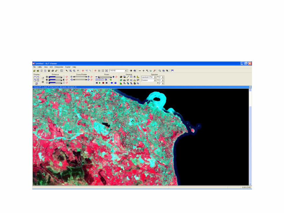
BAD
Chose the algotithm that will
allocate pixels into your classess
Some Types of Classifiers
bull Non-parametric
ndash Parallelepiped classifier (BOX or PPD)
ndash Minimum-distance-to-means (MDM)
ndash Expert Systems
Parametric
ndash Maximum likelihood (ML)
ndash Neural networks
A parametric signature is based on statistical parameters (eg mean and covariance
matrix) of the pixels that are in the training sample or cluster Supervised and
unsupervised training can generate parametric signatures A set of parametric
signatures can be used to train a statistically-based classifier to define the classes
A nonparametric signature is not based on statistics but on discrete objects (polygons or
rectangles) in a feature space image These feature space objects are used to define
the boundaries for the classes
A nonparametric classifier uses a set of nonparametric signatures to assign pixels to a
class based on their location either inside or outside the
area in the feature space image Supervised training is used to generate nonparametric
signatures (Kloer 1994)
Parallelepiped
bull The minimum and maximum DNs for each class are determined and are used as thresholds for classifying the image
bull Benefits simple to train and use computationally fast
bull Drawbacks pixels in the gaps between the parallelepipes can not be classified pixels in the region of overlapping parallelepipes can not be classified
Feature Space tools enable you to interactively define feature
space objects in the feature space image(s) A feature space image is simply a
graph of the data file values of one band of data against the values of another
band (often called a scatterplot)
Parallelepiped
Minimum-Distance-to-Means
Candidate Pixel
to be classified
Class 1 means
Class 2 means
Band 2
Band 1
D1
D2
D1 lt D2 so the pixel is classified
as Class 1
Maximum Likelihood
Machine Learning
Random Forest and Support Vector Machines
bull These techniques whilst easily applied
are beyond the technical scope of this
short course
bull However we have shown the RF is the
best suited method for Irish mapping
MERMS 12 - L4
You can try these methods
using SAGA a free GIS that is
also compatible with ArcGIS
MERMS 12 - L4
httpwwwsaga-gisorgenindexhtml
From Pixels to Objects
Previously we have looked at classification based
only on the spectral characteristics of pixels one
by one But the information in an image isnt
encoded in pixels but objects- things we
recognise
Objects are things on the
Ground
bull Object Orientated Classifcation attempts
to bring to gether many of the aspects of
image interpreatation that we looked at
early in the course on manual
interpretation of imagery- like shadow
texture context etc
bull But do so in an automated fashion so the
computer can create the outptut
Objects
bull We can have a-priori defined objects ndash
cadastral maps for example (Prime 2 in
the Irish context)
bull Or we can create objects from the image
using segmentation
Unclosed areas
bull What does landcover mean in these
areas
bull How best to record extent and change
bull Classifications havent been finalised- but
will be guided by Helm and Eagle
Internationally Fossit locally and at all
times with practicallity in mind
Segmentation
bull Essentially the segmentation algorithm examines how like its neighbours a pixel is- if pixels are alike they are grouped into objects
bull We can use colour of texture or the shape of the object to help us segment an image- most popular software for soing this is e-cognition
bull Its very simalr to the human interpreation approach of mapping ldquophotomorphic regionsrdquo and has been developed out of machine vision reserach
These segments become objects
bull WE can then xclassify the object suing any of
the classifcation we have looked at
bull Unsupervised
bull Supervised
bull Rule based or descsion tree
bull We can also include non-spectral data eg the
size of the object or its shape the variation of
pixels within an object (texture)
Scale15
Color02
Scale15
Color035
Scale50
Color02
Scale15
Color05
bull 22 OBIA Strengths
bull 1048707 Partitioning an image into objects is akin to the way
bull humans conceptually organize the landscape to
bull comprehend it
bull 1048707 Using image-objects as basic units reduces computational
bull classifier and at the sametime enables the user to take advantage of more complex
bull techniques (eg non-parametric)
bull 1048707 Image-objects exhibit useful features that single pixels lack
bull 1048707 Image-objects can be more readily integrated in vector
bull GIS
bull 23 OBIA Weaknesses
bull 1048707 There are numerous challenges involved in processing
bull very large datasets Even if OBIA is more efficient than
bull pixel-based approaches segmenting a multispectral image
bull of several tens of mega-pixels is a formidable task
bull 1048707 Segmentation is an ill-posed problem in the sense it has
bull no unique solution
bull 1048707 There exists a poor understanding of scale and hierarchical
bull relations among objects derived at different resolutions
bull Do segments at coarse resolutions really lsquoemergersquo or
bull lsquoevolversquo from the ones at finer resolutions Should
bull boundaries perfectly overlap (coincide) through scale
bull Operationally itrsquos very appealing but what is the
bull ecological basis for this
httpdesktoparcgiscomenarcmap103toolsspatial-
analyst-toolboxunderstanding-segmentation-and-
classificationhtm
bull The Classify Raster tool performs an image classification as
specified by the Esri classifier definition file Inputs to the tool include the image to be classified the optional segmented raster (such as another raster dataset or a layer such as a DEM) and a classifier definition file to generate the classified raster dataset Note that the Classify Raster tool contains all the supported classifiers The proper classifier is utilized depending on the properties and information contained in the classifier definition file So the classifier definition file generated by the Train ISO Cluster Classifier Train Maximum Likelihood Classifier or Train Support Vector Machine Classifier will activate the corresponding classifier when you run Classify Raster
Purposes of Field Data
bull To verify evaluate or assess the results of
remote sensing investigations (accuracy
assessment)
bull Provide data to geographically correct imagery
bull Provide information used to model the spectral
behaviour of landscape features (plants soils or
waterbodies)
Field data includes least three
kinds of information
bull Attributes or measurements that describe
ground conditions at a specific place
bull Observations must be linked to locational
information so the attributes can be
correctly matched to corresponding points
in image data
bull Observations must also be described with
respect to time and date
Geographic Sampling
bull Observation signifies the selection of a specific cell or pixel
bull Sample is used here to designate a set of observations that will be used in an error matrix
bull Three separate decisions must be made when sampling maps or spatial patterns
bull (1) Number of observations to be used
bull (2) Sampling pattern to position observations within an image
bull (3) Spacing of observations
Numbers of Observations
bull Number of observations determines
ndash the confidence interval of an estimate of the
accuracy of a classification A large sample size
decreases the width of the confidence interval of
our estimate of a statistic
bull For most purposes it is necessary to have
some minimum number of observations
assigned to each class
Sampling Pattern
The Simple Random Sampling Pattern
bull The choice of any specific location as the site for an observation is independent of the selection of any other location as an observation
bull All portions of a region are equally subject to selection for the sample thereby yielding data that accurately represent the area examined and satisfying one of the fundamental requirements of inferential statistics
The Stratified Random Pattern
bull Assigns observations to sub-regions of the image to ensure that the sampling effort is distributed in a rational manner A stratified sampling effort might plan to assign specific number of observations to each category on a map to be evaluated This procedure would ensure that every category would be sampled
bull
Systematic Patterns
This pattern positions
samples such that
observations are taken
at equal intervals
according to a specific
strategy Systematic
sampling is useful if it is
necessary to ensure
that all regions within a
study area are
represented
Systematic Stratified Unaligned Patterns
bull This pattern combines features of both systematic and stratified samples while simultaneously preserving an element of randomness
bull The entire study area is divided into uniform cells
bull The grid cells introduce a systematic component to the sample and form the basis for the stratification one observation is placed in each cell
bull An element of randomness is contributed by the method of placing observations within each cell
Cluster Sampling
bull Cluster Sampling selects points within a study area and uses each point as a centre to determine locations of additional ldquosatelliterdquo observations placed nearby so that the overall distribution of observations forms a clustered pattern
Cluster sampling may be efficient with respect to
time and finance If the pattern to be sampled is
known beforehand it may provide reasonably
accurate results
LOCATIONAL INFORMATION
bull Identification of Ground Control Points (GCPs) which allow analysts to resample image data to provide accurate planimetric location and correctly match image detail to maps and other images
bull Often we would use points of a map (sayu road intersections) to geometrically correct an Image but in some cases we have to identify a feature on the image and go out and survey that point on the ground in order to get accutare geographci correction
bull Additional information from
bull httpeuropaeuintcommspaceindex_enhtml
bull httpeuropaeuintcommdgsenergy_transportgalileo
bull httpwwwgalileojucom
bull httpwwwesaintesaNAgalileohtml
bull httpwwwosiiewp-contentuploads201507Survey-
Ireland-2004-GPS-Network-RTK-Solution-for-
Irelandpdfext=pdf
Accuracy Assessment
We may define accuracy in a working sense as the degree of correspondence between
observation and reality We usually judge accuracy against existing maps large scale aerial photos
or field checks We can pose two fundamental questions about accuracy
Is each category in a classification really present at the points specified on a map
Are the boundaries separating categories valid as located
Various types of errors diminish the accuracy of feature identification and category distribution We
make most of the errors either in measuring or in sampling When quantifying accuracy we must
adjust for the lack of equivalence and totality if possible Another often overlooked point about
maps as reference standards concerns their intrinsic or absolute accuracy Maps require an
independent frame of reference to establish their own validity
As a general rule the level of accuracy obtainable in a remote sensing classification depends on
diverse factors such as the suitability of training sites the size shape distribution and frequency
of occurrence of individual areas assigned to each class the sensor performance and resolution
and the methods involved in classifying (visual photointerpreting versus computer-aided statistical
classifying) and others
In practice we may test classification accuracy in four ways
1) field checks at selected points (usually non-rigorous and subjective) chosen either at
random or along a grid
2) estimate (non-rigorous) the agreement of the theme or class identity between a class
map and reference maps determined usually by overlaying one on the other(s)
3) statistical analysis (rigorous) of numerical data developed in sampling measuring and
processing data using tests such as root mean square standard error analysis of
variance correlation coefficients linear or multiple regression analysis and Chi-square
testing
4) confusion matrix calculations (rigorous)
With the class identities in the photo as the standard we arranged the number of pixels
correctly assigned to each class and those misassigned to other classes in the confusion
matrix listing errors of commission omission and overall accuracies
The producers accuracy relates to the probability that a reference sample (photo-
interpreted land cover class in this project) will be correctly mapped and measures
the errors of omission (1 - producers accuracy)
In contrast the users accuracy indicates the probability that a sample from land
cover map actually matches what it is from the reference data (photo-interpreted
land cover class in this project) and measures the error of commission (1- uses
accuracy)
Errors of commission An error of commission results when a pixel is committed to an
incorrect class
Errors of omission An error of omission results when a pixel is incorrectly classified
into another category The pixel is omitted from its correct class
urban grass natural water forestry map
urban 12 5 1 6 7 31
grass 1 34 7 2 44
natural 2 9 23 6 40
water 14 2 16
forestry 4 20 24
ground
15 48 31 24 37 155
Urban Ommission (31-12)31= 61
So Producers accuracy is 39
Urban Comission (15-12)15= 25
So users accuracy is 75
Total mapp accuray is (12+34+23+14+20)155 = 66

Parallelepiped
bull The minimum and maximum DNs for each class are determined and are used as thresholds for classifying the image
bull Benefits simple to train and use computationally fast
bull Drawbacks pixels in the gaps between the parallelepipes can not be classified pixels in the region of overlapping parallelepipes can not be classified
Feature Space tools enable you to interactively define feature
space objects in the feature space image(s) A feature space image is simply a
graph of the data file values of one band of data against the values of another
band (often called a scatterplot)
Parallelepiped
Minimum-Distance-to-Means
Candidate Pixel
to be classified
Class 1 means
Class 2 means
Band 2
Band 1
D1
D2
D1 lt D2 so the pixel is classified
as Class 1
Maximum Likelihood
Machine Learning
Random Forest and Support Vector Machines
bull These techniques whilst easily applied
are beyond the technical scope of this
short course
bull However we have shown the RF is the
best suited method for Irish mapping
MERMS 12 - L4
You can try these methods
using SAGA a free GIS that is
also compatible with ArcGIS
MERMS 12 - L4
httpwwwsaga-gisorgenindexhtml
From Pixels to Objects
Previously we have looked at classification based
only on the spectral characteristics of pixels one
by one But the information in an image isnt
encoded in pixels but objects- things we
recognise
Objects are things on the
Ground
bull Object Orientated Classifcation attempts
to bring to gether many of the aspects of
image interpreatation that we looked at
early in the course on manual
interpretation of imagery- like shadow
texture context etc
bull But do so in an automated fashion so the
computer can create the outptut
Objects
bull We can have a-priori defined objects ndash
cadastral maps for example (Prime 2 in
the Irish context)
bull Or we can create objects from the image
using segmentation
Unclosed areas
bull What does landcover mean in these
areas
bull How best to record extent and change
bull Classifications havent been finalised- but
will be guided by Helm and Eagle
Internationally Fossit locally and at all
times with practicallity in mind
Segmentation
bull Essentially the segmentation algorithm examines how like its neighbours a pixel is- if pixels are alike they are grouped into objects
bull We can use colour of texture or the shape of the object to help us segment an image- most popular software for soing this is e-cognition
bull Its very simalr to the human interpreation approach of mapping ldquophotomorphic regionsrdquo and has been developed out of machine vision reserach
These segments become objects
bull WE can then xclassify the object suing any of
the classifcation we have looked at
bull Unsupervised
bull Supervised
bull Rule based or descsion tree
bull We can also include non-spectral data eg the
size of the object or its shape the variation of
pixels within an object (texture)
Scale15
Color02
Scale15
Color035
Scale50
Color02
Scale15
Color05
bull 22 OBIA Strengths
bull 1048707 Partitioning an image into objects is akin to the way
bull humans conceptually organize the landscape to
bull comprehend it
bull 1048707 Using image-objects as basic units reduces computational
bull classifier and at the sametime enables the user to take advantage of more complex
bull techniques (eg non-parametric)
bull 1048707 Image-objects exhibit useful features that single pixels lack
bull 1048707 Image-objects can be more readily integrated in vector
bull GIS
bull 23 OBIA Weaknesses
bull 1048707 There are numerous challenges involved in processing
bull very large datasets Even if OBIA is more efficient than
bull pixel-based approaches segmenting a multispectral image
bull of several tens of mega-pixels is a formidable task
bull 1048707 Segmentation is an ill-posed problem in the sense it has
bull no unique solution
bull 1048707 There exists a poor understanding of scale and hierarchical
bull relations among objects derived at different resolutions
bull Do segments at coarse resolutions really lsquoemergersquo or
bull lsquoevolversquo from the ones at finer resolutions Should
bull boundaries perfectly overlap (coincide) through scale
bull Operationally itrsquos very appealing but what is the
bull ecological basis for this
httpdesktoparcgiscomenarcmap103toolsspatial-
analyst-toolboxunderstanding-segmentation-and-
classificationhtm
bull The Classify Raster tool performs an image classification as
specified by the Esri classifier definition file Inputs to the tool include the image to be classified the optional segmented raster (such as another raster dataset or a layer such as a DEM) and a classifier definition file to generate the classified raster dataset Note that the Classify Raster tool contains all the supported classifiers The proper classifier is utilized depending on the properties and information contained in the classifier definition file So the classifier definition file generated by the Train ISO Cluster Classifier Train Maximum Likelihood Classifier or Train Support Vector Machine Classifier will activate the corresponding classifier when you run Classify Raster
Purposes of Field Data
bull To verify evaluate or assess the results of
remote sensing investigations (accuracy
assessment)
bull Provide data to geographically correct imagery
bull Provide information used to model the spectral
behaviour of landscape features (plants soils or
waterbodies)
Field data includes least three
kinds of information
bull Attributes or measurements that describe
ground conditions at a specific place
bull Observations must be linked to locational
information so the attributes can be
correctly matched to corresponding points
in image data
bull Observations must also be described with
respect to time and date
Geographic Sampling
bull Observation signifies the selection of a specific cell or pixel
bull Sample is used here to designate a set of observations that will be used in an error matrix
bull Three separate decisions must be made when sampling maps or spatial patterns
bull (1) Number of observations to be used
bull (2) Sampling pattern to position observations within an image
bull (3) Spacing of observations
Numbers of Observations
bull Number of observations determines
ndash the confidence interval of an estimate of the
accuracy of a classification A large sample size
decreases the width of the confidence interval of
our estimate of a statistic
bull For most purposes it is necessary to have
some minimum number of observations
assigned to each class
Sampling Pattern
The Simple Random Sampling Pattern
bull The choice of any specific location as the site for an observation is independent of the selection of any other location as an observation
bull All portions of a region are equally subject to selection for the sample thereby yielding data that accurately represent the area examined and satisfying one of the fundamental requirements of inferential statistics
The Stratified Random Pattern
bull Assigns observations to sub-regions of the image to ensure that the sampling effort is distributed in a rational manner A stratified sampling effort might plan to assign specific number of observations to each category on a map to be evaluated This procedure would ensure that every category would be sampled
bull
Systematic Patterns
This pattern positions
samples such that
observations are taken
at equal intervals
according to a specific
strategy Systematic
sampling is useful if it is
necessary to ensure
that all regions within a
study area are
represented
Systematic Stratified Unaligned Patterns
bull This pattern combines features of both systematic and stratified samples while simultaneously preserving an element of randomness
bull The entire study area is divided into uniform cells
bull The grid cells introduce a systematic component to the sample and form the basis for the stratification one observation is placed in each cell
bull An element of randomness is contributed by the method of placing observations within each cell
Cluster Sampling
bull Cluster Sampling selects points within a study area and uses each point as a centre to determine locations of additional ldquosatelliterdquo observations placed nearby so that the overall distribution of observations forms a clustered pattern
Cluster sampling may be efficient with respect to
time and finance If the pattern to be sampled is
known beforehand it may provide reasonably
accurate results
LOCATIONAL INFORMATION
bull Identification of Ground Control Points (GCPs) which allow analysts to resample image data to provide accurate planimetric location and correctly match image detail to maps and other images
bull Often we would use points of a map (sayu road intersections) to geometrically correct an Image but in some cases we have to identify a feature on the image and go out and survey that point on the ground in order to get accutare geographci correction
bull Additional information from
bull httpeuropaeuintcommspaceindex_enhtml
bull httpeuropaeuintcommdgsenergy_transportgalileo
bull httpwwwgalileojucom
bull httpwwwesaintesaNAgalileohtml
bull httpwwwosiiewp-contentuploads201507Survey-
Ireland-2004-GPS-Network-RTK-Solution-for-
Irelandpdfext=pdf
Accuracy Assessment
We may define accuracy in a working sense as the degree of correspondence between
observation and reality We usually judge accuracy against existing maps large scale aerial photos
or field checks We can pose two fundamental questions about accuracy
Is each category in a classification really present at the points specified on a map
Are the boundaries separating categories valid as located
Various types of errors diminish the accuracy of feature identification and category distribution We
make most of the errors either in measuring or in sampling When quantifying accuracy we must
adjust for the lack of equivalence and totality if possible Another often overlooked point about
maps as reference standards concerns their intrinsic or absolute accuracy Maps require an
independent frame of reference to establish their own validity
As a general rule the level of accuracy obtainable in a remote sensing classification depends on
diverse factors such as the suitability of training sites the size shape distribution and frequency
of occurrence of individual areas assigned to each class the sensor performance and resolution
and the methods involved in classifying (visual photointerpreting versus computer-aided statistical
classifying) and others
In practice we may test classification accuracy in four ways
1) field checks at selected points (usually non-rigorous and subjective) chosen either at
random or along a grid
2) estimate (non-rigorous) the agreement of the theme or class identity between a class
map and reference maps determined usually by overlaying one on the other(s)
3) statistical analysis (rigorous) of numerical data developed in sampling measuring and
processing data using tests such as root mean square standard error analysis of
variance correlation coefficients linear or multiple regression analysis and Chi-square
testing
4) confusion matrix calculations (rigorous)
With the class identities in the photo as the standard we arranged the number of pixels
correctly assigned to each class and those misassigned to other classes in the confusion
matrix listing errors of commission omission and overall accuracies
The producers accuracy relates to the probability that a reference sample (photo-
interpreted land cover class in this project) will be correctly mapped and measures
the errors of omission (1 - producers accuracy)
In contrast the users accuracy indicates the probability that a sample from land
cover map actually matches what it is from the reference data (photo-interpreted
land cover class in this project) and measures the error of commission (1- uses
accuracy)
Errors of commission An error of commission results when a pixel is committed to an
incorrect class
Errors of omission An error of omission results when a pixel is incorrectly classified
into another category The pixel is omitted from its correct class
urban grass natural water forestry map
urban 12 5 1 6 7 31
grass 1 34 7 2 44
natural 2 9 23 6 40
water 14 2 16
forestry 4 20 24
ground
15 48 31 24 37 155
Urban Ommission (31-12)31= 61
So Producers accuracy is 39
Urban Comission (15-12)15= 25
So users accuracy is 75
Total mapp accuray is (12+34+23+14+20)155 = 66
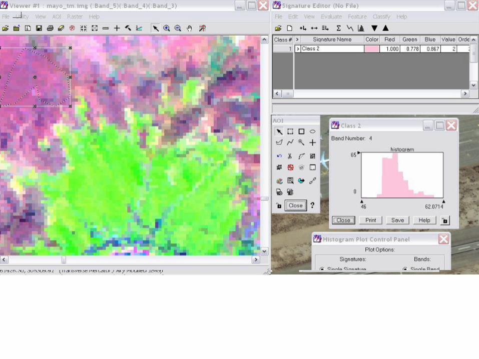
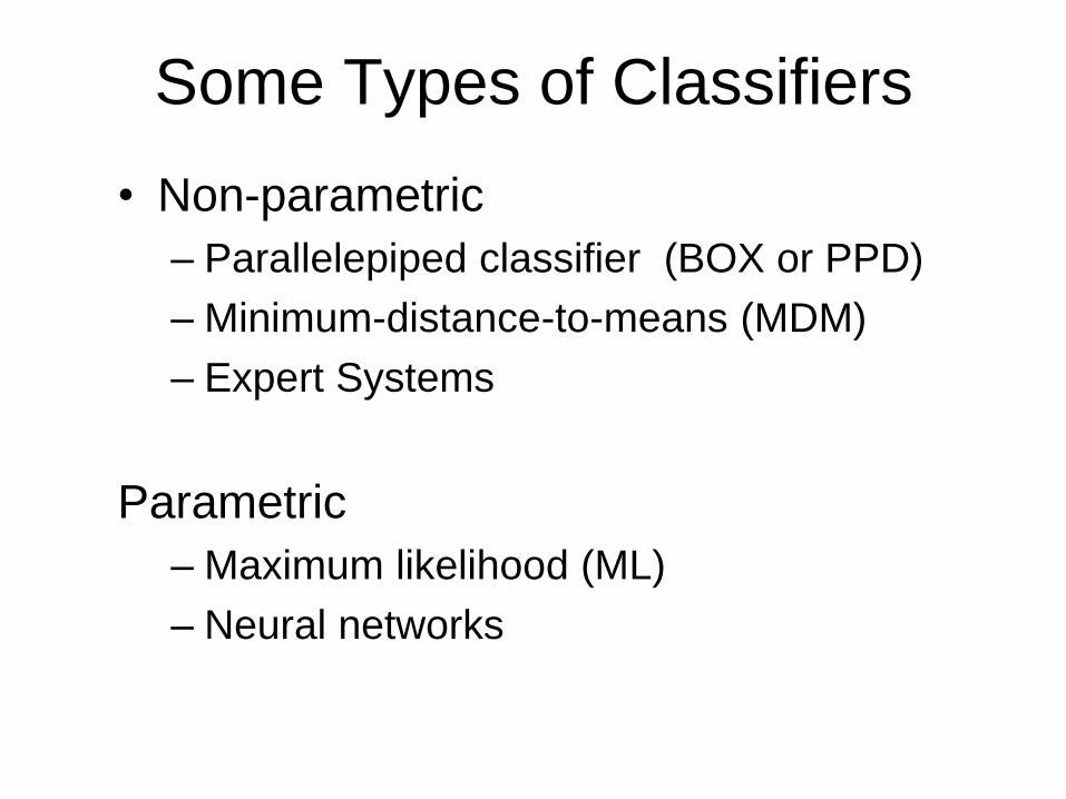
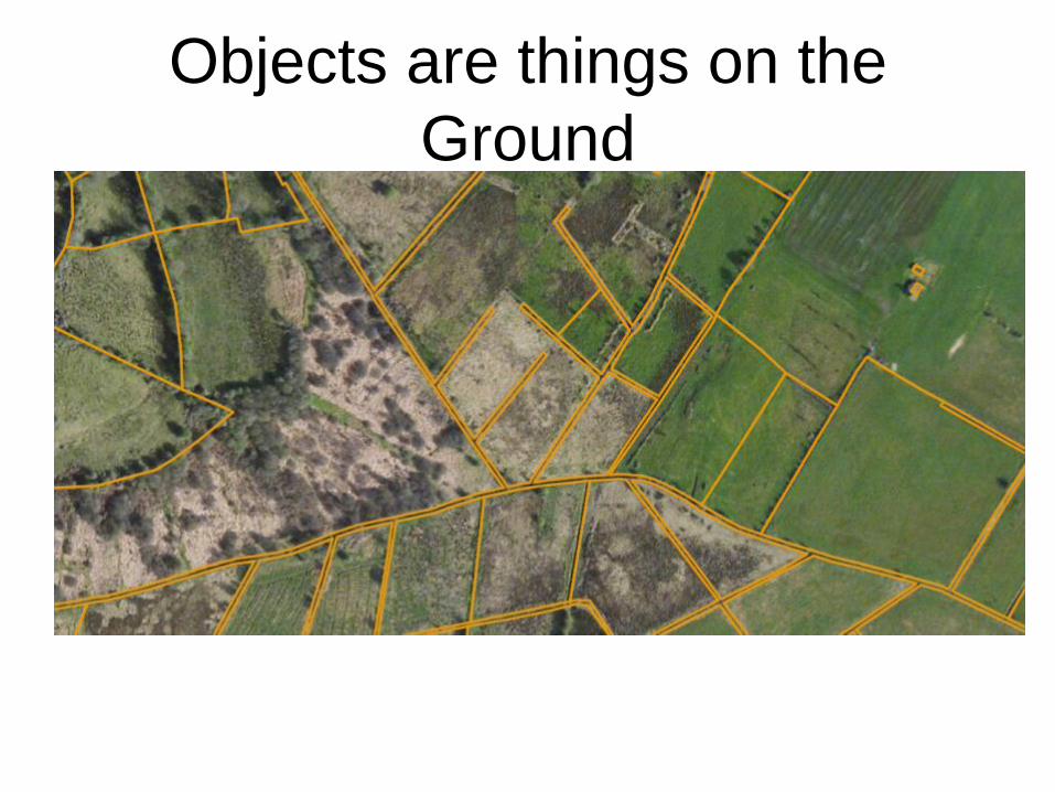

Scale15
Color02
Scale15
Color035
Scale50
Color02
Scale15
Color05
bull 22 OBIA Strengths
bull 1048707 Partitioning an image into objects is akin to the way
bull humans conceptually organize the landscape to
bull comprehend it
bull 1048707 Using image-objects as basic units reduces computational
bull classifier and at the sametime enables the user to take advantage of more complex
bull techniques (eg non-parametric)
bull 1048707 Image-objects exhibit useful features that single pixels lack
bull 1048707 Image-objects can be more readily integrated in vector
bull GIS
bull 23 OBIA Weaknesses
bull 1048707 There are numerous challenges involved in processing
bull very large datasets Even if OBIA is more efficient than
bull pixel-based approaches segmenting a multispectral image
bull of several tens of mega-pixels is a formidable task
bull 1048707 Segmentation is an ill-posed problem in the sense it has
bull no unique solution
bull 1048707 There exists a poor understanding of scale and hierarchical
bull relations among objects derived at different resolutions
bull Do segments at coarse resolutions really lsquoemergersquo or
bull lsquoevolversquo from the ones at finer resolutions Should
bull boundaries perfectly overlap (coincide) through scale
bull Operationally itrsquos very appealing but what is the
bull ecological basis for this
httpdesktoparcgiscomenarcmap103toolsspatial-
analyst-toolboxunderstanding-segmentation-and-
classificationhtm
bull The Classify Raster tool performs an image classification as
specified by the Esri classifier definition file Inputs to the tool include the image to be classified the optional segmented raster (such as another raster dataset or a layer such as a DEM) and a classifier definition file to generate the classified raster dataset Note that the Classify Raster tool contains all the supported classifiers The proper classifier is utilized depending on the properties and information contained in the classifier definition file So the classifier definition file generated by the Train ISO Cluster Classifier Train Maximum Likelihood Classifier or Train Support Vector Machine Classifier will activate the corresponding classifier when you run Classify Raster
Purposes of Field Data
bull To verify evaluate or assess the results of
remote sensing investigations (accuracy
assessment)
bull Provide data to geographically correct imagery
bull Provide information used to model the spectral
behaviour of landscape features (plants soils or
waterbodies)
Field data includes least three
kinds of information
bull Attributes or measurements that describe
ground conditions at a specific place
bull Observations must be linked to locational
information so the attributes can be
correctly matched to corresponding points
in image data
bull Observations must also be described with
respect to time and date
Geographic Sampling
bull Observation signifies the selection of a specific cell or pixel
bull Sample is used here to designate a set of observations that will be used in an error matrix
bull Three separate decisions must be made when sampling maps or spatial patterns
bull (1) Number of observations to be used
bull (2) Sampling pattern to position observations within an image
bull (3) Spacing of observations
Numbers of Observations
bull Number of observations determines
ndash the confidence interval of an estimate of the
accuracy of a classification A large sample size
decreases the width of the confidence interval of
our estimate of a statistic
bull For most purposes it is necessary to have
some minimum number of observations
assigned to each class
Sampling Pattern
The Simple Random Sampling Pattern
bull The choice of any specific location as the site for an observation is independent of the selection of any other location as an observation
bull All portions of a region are equally subject to selection for the sample thereby yielding data that accurately represent the area examined and satisfying one of the fundamental requirements of inferential statistics
The Stratified Random Pattern
bull Assigns observations to sub-regions of the image to ensure that the sampling effort is distributed in a rational manner A stratified sampling effort might plan to assign specific number of observations to each category on a map to be evaluated This procedure would ensure that every category would be sampled
bull
Systematic Patterns
This pattern positions
samples such that
observations are taken
at equal intervals
according to a specific
strategy Systematic
sampling is useful if it is
necessary to ensure
that all regions within a
study area are
represented
Systematic Stratified Unaligned Patterns
bull This pattern combines features of both systematic and stratified samples while simultaneously preserving an element of randomness
bull The entire study area is divided into uniform cells
bull The grid cells introduce a systematic component to the sample and form the basis for the stratification one observation is placed in each cell
bull An element of randomness is contributed by the method of placing observations within each cell
Cluster Sampling
bull Cluster Sampling selects points within a study area and uses each point as a centre to determine locations of additional ldquosatelliterdquo observations placed nearby so that the overall distribution of observations forms a clustered pattern
Cluster sampling may be efficient with respect to
time and finance If the pattern to be sampled is
known beforehand it may provide reasonably
accurate results
LOCATIONAL INFORMATION
bull Identification of Ground Control Points (GCPs) which allow analysts to resample image data to provide accurate planimetric location and correctly match image detail to maps and other images
bull Often we would use points of a map (sayu road intersections) to geometrically correct an Image but in some cases we have to identify a feature on the image and go out and survey that point on the ground in order to get accutare geographci correction
bull Additional information from
bull httpeuropaeuintcommspaceindex_enhtml
bull httpeuropaeuintcommdgsenergy_transportgalileo
bull httpwwwgalileojucom
bull httpwwwesaintesaNAgalileohtml
bull httpwwwosiiewp-contentuploads201507Survey-
Ireland-2004-GPS-Network-RTK-Solution-for-
Irelandpdfext=pdf
Accuracy Assessment
We may define accuracy in a working sense as the degree of correspondence between
observation and reality We usually judge accuracy against existing maps large scale aerial photos
or field checks We can pose two fundamental questions about accuracy
Is each category in a classification really present at the points specified on a map
Are the boundaries separating categories valid as located
Various types of errors diminish the accuracy of feature identification and category distribution We
make most of the errors either in measuring or in sampling When quantifying accuracy we must
adjust for the lack of equivalence and totality if possible Another often overlooked point about
maps as reference standards concerns their intrinsic or absolute accuracy Maps require an
independent frame of reference to establish their own validity
As a general rule the level of accuracy obtainable in a remote sensing classification depends on
diverse factors such as the suitability of training sites the size shape distribution and frequency
of occurrence of individual areas assigned to each class the sensor performance and resolution
and the methods involved in classifying (visual photointerpreting versus computer-aided statistical
classifying) and others
In practice we may test classification accuracy in four ways
1) field checks at selected points (usually non-rigorous and subjective) chosen either at
random or along a grid
2) estimate (non-rigorous) the agreement of the theme or class identity between a class
map and reference maps determined usually by overlaying one on the other(s)
3) statistical analysis (rigorous) of numerical data developed in sampling measuring and
processing data using tests such as root mean square standard error analysis of
variance correlation coefficients linear or multiple regression analysis and Chi-square
testing
4) confusion matrix calculations (rigorous)
With the class identities in the photo as the standard we arranged the number of pixels
correctly assigned to each class and those misassigned to other classes in the confusion
matrix listing errors of commission omission and overall accuracies
The producers accuracy relates to the probability that a reference sample (photo-
interpreted land cover class in this project) will be correctly mapped and measures
the errors of omission (1 - producers accuracy)
In contrast the users accuracy indicates the probability that a sample from land
cover map actually matches what it is from the reference data (photo-interpreted
land cover class in this project) and measures the error of commission (1- uses
accuracy)
Errors of commission An error of commission results when a pixel is committed to an
incorrect class
Errors of omission An error of omission results when a pixel is incorrectly classified
into another category The pixel is omitted from its correct class
urban grass natural water forestry map
urban 12 5 1 6 7 31
grass 1 34 7 2 44
natural 2 9 23 6 40
water 14 2 16
forestry 4 20 24
ground
15 48 31 24 37 155
Urban Ommission (31-12)31= 61
So Producers accuracy is 39
Urban Comission (15-12)15= 25
So users accuracy is 75
Total mapp accuray is (12+34+23+14+20)155 = 66
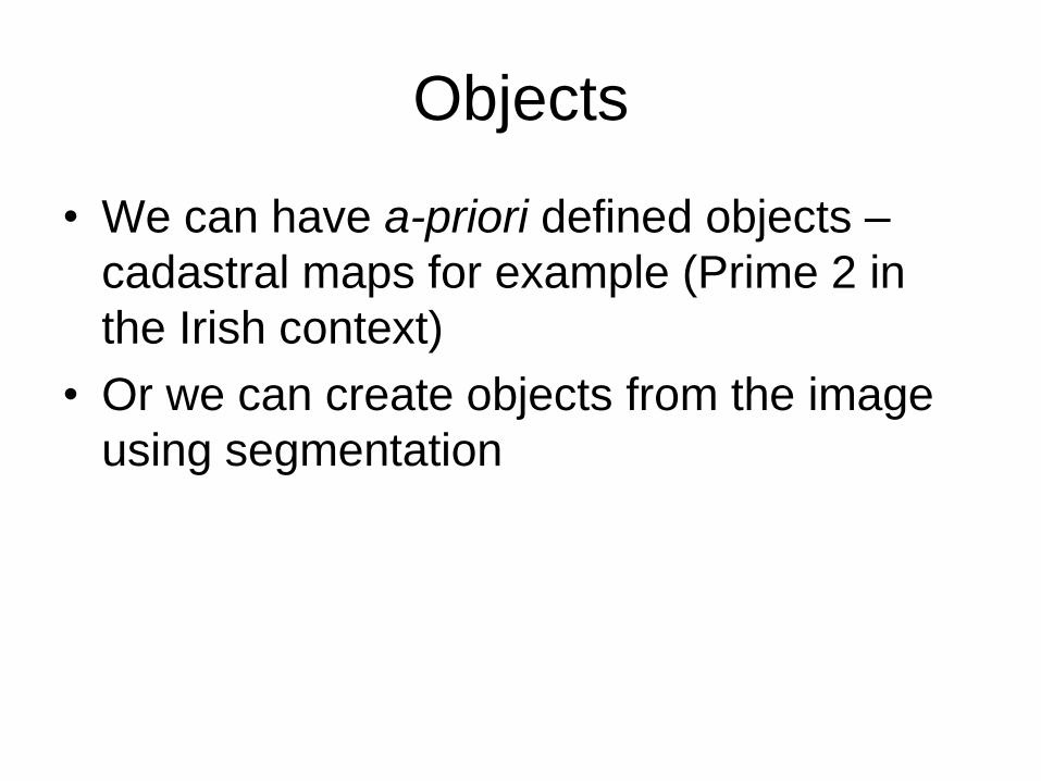
Scale15
Color035
Scale50
Color02
Scale15
Color05
bull 22 OBIA Strengths
bull 1048707 Partitioning an image into objects is akin to the way
bull humans conceptually organize the landscape to
bull comprehend it
bull 1048707 Using image-objects as basic units reduces computational
bull classifier and at the sametime enables the user to take advantage of more complex
bull techniques (eg non-parametric)
bull 1048707 Image-objects exhibit useful features that single pixels lack
bull 1048707 Image-objects can be more readily integrated in vector
bull GIS
bull 23 OBIA Weaknesses
bull 1048707 There are numerous challenges involved in processing
bull very large datasets Even if OBIA is more efficient than
bull pixel-based approaches segmenting a multispectral image
bull of several tens of mega-pixels is a formidable task
bull 1048707 Segmentation is an ill-posed problem in the sense it has
bull no unique solution
bull 1048707 There exists a poor understanding of scale and hierarchical
bull relations among objects derived at different resolutions
bull Do segments at coarse resolutions really lsquoemergersquo or
bull lsquoevolversquo from the ones at finer resolutions Should
bull boundaries perfectly overlap (coincide) through scale
bull Operationally itrsquos very appealing but what is the
bull ecological basis for this
httpdesktoparcgiscomenarcmap103toolsspatial-
analyst-toolboxunderstanding-segmentation-and-
classificationhtm
bull The Classify Raster tool performs an image classification as
specified by the Esri classifier definition file Inputs to the tool include the image to be classified the optional segmented raster (such as another raster dataset or a layer such as a DEM) and a classifier definition file to generate the classified raster dataset Note that the Classify Raster tool contains all the supported classifiers The proper classifier is utilized depending on the properties and information contained in the classifier definition file So the classifier definition file generated by the Train ISO Cluster Classifier Train Maximum Likelihood Classifier or Train Support Vector Machine Classifier will activate the corresponding classifier when you run Classify Raster
Purposes of Field Data
bull To verify evaluate or assess the results of
remote sensing investigations (accuracy
assessment)
bull Provide data to geographically correct imagery
bull Provide information used to model the spectral
behaviour of landscape features (plants soils or
waterbodies)
Field data includes least three
kinds of information
bull Attributes or measurements that describe
ground conditions at a specific place
bull Observations must be linked to locational
information so the attributes can be
correctly matched to corresponding points
in image data
bull Observations must also be described with
respect to time and date
Geographic Sampling
bull Observation signifies the selection of a specific cell or pixel
bull Sample is used here to designate a set of observations that will be used in an error matrix
bull Three separate decisions must be made when sampling maps or spatial patterns
bull (1) Number of observations to be used
bull (2) Sampling pattern to position observations within an image
bull (3) Spacing of observations
Numbers of Observations
bull Number of observations determines
ndash the confidence interval of an estimate of the
accuracy of a classification A large sample size
decreases the width of the confidence interval of
our estimate of a statistic
bull For most purposes it is necessary to have
some minimum number of observations
assigned to each class
Sampling Pattern
The Simple Random Sampling Pattern
bull The choice of any specific location as the site for an observation is independent of the selection of any other location as an observation
bull All portions of a region are equally subject to selection for the sample thereby yielding data that accurately represent the area examined and satisfying one of the fundamental requirements of inferential statistics
The Stratified Random Pattern
bull Assigns observations to sub-regions of the image to ensure that the sampling effort is distributed in a rational manner A stratified sampling effort might plan to assign specific number of observations to each category on a map to be evaluated This procedure would ensure that every category would be sampled
bull
Systematic Patterns
This pattern positions
samples such that
observations are taken
at equal intervals
according to a specific
strategy Systematic
sampling is useful if it is
necessary to ensure
that all regions within a
study area are
represented
Systematic Stratified Unaligned Patterns
bull This pattern combines features of both systematic and stratified samples while simultaneously preserving an element of randomness
bull The entire study area is divided into uniform cells
bull The grid cells introduce a systematic component to the sample and form the basis for the stratification one observation is placed in each cell
bull An element of randomness is contributed by the method of placing observations within each cell
Cluster Sampling
bull Cluster Sampling selects points within a study area and uses each point as a centre to determine locations of additional ldquosatelliterdquo observations placed nearby so that the overall distribution of observations forms a clustered pattern
Cluster sampling may be efficient with respect to
time and finance If the pattern to be sampled is
known beforehand it may provide reasonably
accurate results
LOCATIONAL INFORMATION
bull Identification of Ground Control Points (GCPs) which allow analysts to resample image data to provide accurate planimetric location and correctly match image detail to maps and other images
bull Often we would use points of a map (sayu road intersections) to geometrically correct an Image but in some cases we have to identify a feature on the image and go out and survey that point on the ground in order to get accutare geographci correction
bull Additional information from
bull httpeuropaeuintcommspaceindex_enhtml
bull httpeuropaeuintcommdgsenergy_transportgalileo
bull httpwwwgalileojucom
bull httpwwwesaintesaNAgalileohtml
bull httpwwwosiiewp-contentuploads201507Survey-
Ireland-2004-GPS-Network-RTK-Solution-for-
Irelandpdfext=pdf
Accuracy Assessment
We may define accuracy in a working sense as the degree of correspondence between
observation and reality We usually judge accuracy against existing maps large scale aerial photos
or field checks We can pose two fundamental questions about accuracy
Is each category in a classification really present at the points specified on a map
Are the boundaries separating categories valid as located
Various types of errors diminish the accuracy of feature identification and category distribution We
make most of the errors either in measuring or in sampling When quantifying accuracy we must
adjust for the lack of equivalence and totality if possible Another often overlooked point about
maps as reference standards concerns their intrinsic or absolute accuracy Maps require an
independent frame of reference to establish their own validity
As a general rule the level of accuracy obtainable in a remote sensing classification depends on
diverse factors such as the suitability of training sites the size shape distribution and frequency
of occurrence of individual areas assigned to each class the sensor performance and resolution
and the methods involved in classifying (visual photointerpreting versus computer-aided statistical
classifying) and others
In practice we may test classification accuracy in four ways
1) field checks at selected points (usually non-rigorous and subjective) chosen either at
random or along a grid
2) estimate (non-rigorous) the agreement of the theme or class identity between a class
map and reference maps determined usually by overlaying one on the other(s)
3) statistical analysis (rigorous) of numerical data developed in sampling measuring and
processing data using tests such as root mean square standard error analysis of
variance correlation coefficients linear or multiple regression analysis and Chi-square
testing
4) confusion matrix calculations (rigorous)
With the class identities in the photo as the standard we arranged the number of pixels
correctly assigned to each class and those misassigned to other classes in the confusion
matrix listing errors of commission omission and overall accuracies
The producers accuracy relates to the probability that a reference sample (photo-
interpreted land cover class in this project) will be correctly mapped and measures
the errors of omission (1 - producers accuracy)
In contrast the users accuracy indicates the probability that a sample from land
cover map actually matches what it is from the reference data (photo-interpreted
land cover class in this project) and measures the error of commission (1- uses
accuracy)
Errors of commission An error of commission results when a pixel is committed to an
incorrect class
Errors of omission An error of omission results when a pixel is incorrectly classified
into another category The pixel is omitted from its correct class
urban grass natural water forestry map
urban 12 5 1 6 7 31
grass 1 34 7 2 44
natural 2 9 23 6 40
water 14 2 16
forestry 4 20 24
ground
15 48 31 24 37 155
Urban Ommission (31-12)31= 61
So Producers accuracy is 39
Urban Comission (15-12)15= 25
So users accuracy is 75
Total mapp accuray is (12+34+23+14+20)155 = 66
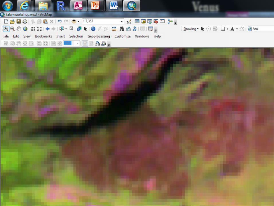
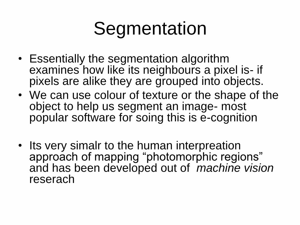
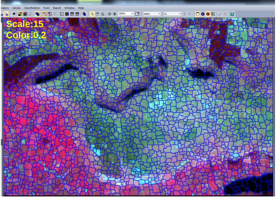
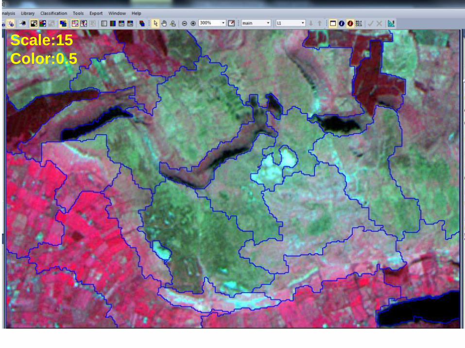
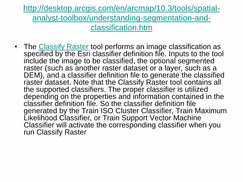
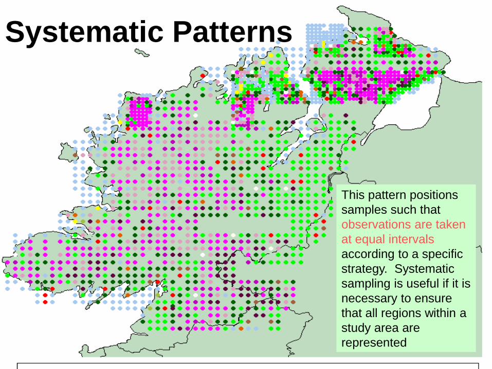
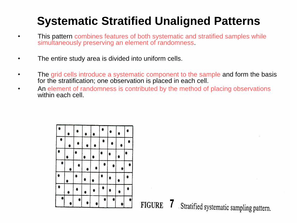