PNNL-17465

Errors and Uncertainties in Dose Reconstruction for Radiation Effects Research DJ Strom April 2008

DISCLAIMER This report was prepared as an account of work sponsored by an agency of the United States Government. Neither the United States Government nor any agency thereof, nor Battelle Memorial Institute, nor any of their employees, makes any warranty, express or implied, or assumes any legal liability or responsibility for the accuracy, completeness, or usefulness of any information, apparatus, product, or process disclosed, or represents that its use would not infringe privately owned rights. Reference herein to any specific commercial product, process, or service by trade name, trademark, manufacturer, or otherwise does not necessarily constitute or imply its endorsement, recommendation, or favoring by the United States Government or any agency thereof, or Battelle Memorial Institute. The views and opinions of authors expressed herein do not necessarily state or reflect those of the United States Government or any agency thereof. PACIFIC NORTHWEST NATIONAL LABORATORY operated by BATTELLE for the UNITED STATES DEPARTMENT OF ENERGY under Contract DE-AC05-76RL01830 Printed in the United States of America Available to DOE and DOE contractors from the Office of Scientific and Technical Information,

P.O. Box 62, Oak Ridge, TN 37831-0062; ph: (865) 576-8401 fax: (865) 576-5728

email: reports@adonis.osti.gov Available to the public from the National Technical Information Service, U.S. Department of Commerce, 5285 Port Royal Rd., Springfield, VA 22161

ph: (800) 553-6847 fax: (703) 605-6900

email: orders@ntis.fedworld.gov online ordering: http://www.ntis.gov/ordering.htm

This document was printed on recycled paper.

(9/2003)

2

PNNL-17465

Errors and Uncertainties in Dose Reconstruction for Radiation Effects Research Daniel J. Strom April 2008

Prepared for the Joint Coordinating Committee for Radiation Effects Research Project 2.4 under U.S. Department of Energy contract DE-AC05-76RL01830 Pacific Northwest National Laboratory Richland, Washington 99352

iv

Contents 1 Introduction........................................................................................................................................... 1 2 Uncertainty and Error ........................................................................................................................... 2

2.1 Terminology: Error and Uncertainty ........................................................................................... 2 2.2 Two Kinds of Errors: Berkson and Classical .............................................................................. 2

2.2.1 Classical Errors ....................................................................................................................... 2 2.2.2 Berkson Errors ........................................................................................................................ 3 2.2.3 Effect of Berkson Errors in Radiation Effects Research ......................................................... 3

2.3 Shared and Unshared Errors ........................................................................................................ 8 2.4 Work on the Techa River Dosimetry System.............................................................................. 9 2.5 Use of Uncertain Dosimetry Results in Epidemiology................................................................ 9

3 Correction Factors............................................................................................................................... 10 3.1 ISO Definitions.......................................................................................................................... 10 3.2 Discussion of Previous Approaches to Correcting Dosimetry Results...................................... 10 3.3 Modification of Previous Approach that Doesn’t Assume that the Arithmetic and Geometric Means of a Lognormal Distribution Are Equal....................................................................................... 12 3.4 Asymmetry of Confidence Intervals about the Mean of a Lognormally-Distributed Variable .13

4 Examples of Contributions to Bias Correction and Uncertainty in Dose Reconstruction .................. 18 4.1 Elements Contributing to Bias and Uncertainty for External Dosimetry .................................. 18

4.1.1 Neutrons ................................................................................................................................ 18 4.1.2 X- and Gamma Radiation...................................................................................................... 20 4.1.3 Medical Radiation Exposures................................................................................................ 21 4.1.4 Intakes of Radionuclides ....................................................................................................... 23

4.2 Residual Systematic Error ......................................................................................................... 23 4.3 Error, Variability, and Uncertainty............................................................................................23

5 Intra-individual Covariance of Annual Doses over Time ................................................................... 24 6 A Proposal for a Numerical Expression of Uncertainty in Results of Dose Reconstruction to Be Applied Throughout JCCRER Project 2.4.................................................................................................. 25

6.1 Specific Proposal for DOSES2008: The Dose-Uncertainty Vector .......................................... 25 6.1.1 Six Dose Categories .............................................................................................................. 25 6.1.2 Component 1: The Corrected Annual Dose DCorr,C,T(i,y)....................................................... 25 6.1.3 Component 2: The Magnitude of the Uncertainty, SG........................................................... 25 6.1.4 Component 3: Apportionment of the Variance in Dose Uncertainty, fClassical........................ 25 6.1.5 Components 4 and 5: Covariance Over Time Expressed as a Correlation Coefficient r2(y) and Correlation Start Year yCrlt(y) ....................................................................................................... 26 6.1.6 The 5-Component Dose-Uncertainty Vector ........................................................................ 26 6.1.7 What Is Not Included in the Dose-Uncertainty Vector ......................................................... 26

6.2 Determining the Uncertainty Parameters of the Dose-Uncertainty Vector ............................... 27 6.3 Use of the Dose-Uncertainty Vector.......................................................................................... 28

6.3.1 Cumulating Organ or Tissue Doses Up to a Certain Year .................................................... 28 6.3.2 Uncertainty Propagation for Cumulated Organ or Tissue Doses .......................................... 28

6.4 Proposed Milestones for the Uncertainty Task.......................................................................... 28 6.5 Level of Effort ........................................................................................................................... 29

7 Acknowledgements............................................................................................................................. 30 8 Appendix A: Terminology .................................................................................................................. 31 9 Appendix B: Propagation of Uncertainty for Lognormally-Distributed Correction Factors .............. 32

9.1 Point Estimates .......................................................................................................................... 32 9.2 Normally-Distributed Correction Factors.................................................................................. 33 9.3 Lognormally-Distributed Correction Factors ............................................................................ 33

v

9.4 General Procedure for Propagating Lognormally Distributed Uncertainties ............................ 33 10 Appendix C: Results that Are Small Compared to Measurement Uncertainty.............................. 36 11 References...................................................................................................................................... 38

1

1 Introduction Dose reconstruction for studies of the health effects of ionizing radiation have been carried out for many decades. Major studies have included Japanese bomb survivors, atomic veterans, downwinders of the Nevada Test Site and Hanford, underground uranium miners, and populations of nuclear workers. For such studies to be credible, significant effort must be put into applying the best science to reconstructing unbiased absorbed doses to tissues and organs as a function of time. In many cases, more and more sophisticated dose reconstruction methods have been developed as studies progressed. For the example of the Japanese bomb survivors, the dose surrogate “distance from the hypocenter” was replaced by slant range, and then by TD65 doses, DS86 doses, and more recently DS02 doses. Over the years, it has become increasingly clear that an equal level of effort must be expended on the quantitative assessment of uncertainty in such doses, and to reducing and managing uncertainty. In this context, this report reviews difficulties in terminology, explores the nature of Berkson and classical uncertainties in dose reconstruction through examples, and proposes a path forward for Joint Coordinating Committee for Radiation Effects Research (JCCRER) Project 2.4 that requires a reasonably small level of effort for DOSES-2008.

2

2 Uncertainty and Error There are some issues of terminology that should be clarified to ensure clear communication. One issue that has received ever increasing attention is the subject of classical and Berkson errors, and the differing effects each has on the inference of dose-response relationships, power, and confidence intervals. Other issues include shared and unshared errors, covariance over time within an individual’s dose history, how uncertainties can be assessed

2.1 Terminology: Error and Uncertainty The International Organization for Standardization has clearly defined metrology terms (International Organization for Standardization (ISO)1995), and these have been adopted by the U.S. National Institute of Standards and Technology (Taylor and Kuyatt1994). The ISO makes careful distinction between the words “error” and “uncertainty.” Error is the “result of a measurement minus the … measurand,” where the measurand is the “true value” of the quantity being measured (ISO 1995 B.2.19). Uncertainty is the “parameter, associated with the result of a measurement, that characterizes the dispersion of the values that could reasonably be attributed to the measurand” (ISO 1995 B.2.18). Since the measurand is unknown and unknowable, so is the error. “The result of a measurement (after correction) can unknowably be very close to the value of the measurand (and hence have negligible error) even though it may have a large uncertainty. Thus the uncertainty of the result of a measurement should not be confused with the remaining unknown error” (ISO 1995 3.3.1). The ISO addresses “correction” of measurement results for known systematic deviations inherent in the measurement process. The ISO (1995) presents methods for assessing combined standard uncertainty to characterize this distribution, including both random and systematic error components. According to the ISO, a Type A uncertainty evaluation is performed by statistical means, such as calculating the standard deviation of a group of repeated measurements. Similarly, a Type B uncertainty evaluation is performed by means other than statistical analysis, such as using expert judgment and process knowledge. The ISO does not discuss inferences from measurements that result from using measurement results in elaborate models, such as those used in radiation dose reconstruction for health studies. Some additional considerations of terminology are given in Appendix A.

2.2 Two Kinds of Errors: Berkson and Classical In 1950, Joseph Berkson published a paper that distinguished two conceptually different kinds of errors (Berkson1950). Berkson discussed the effect such errors have on linear regression, giving examples from physics (voltage, current, and resistance in a DC circuit) and controlled toxicology experiments or clinical trials in which a dose of some agent is administered to groups of subjects.

2.2.1 Classical Errors The first kind of error Berkson describes, now known as a classical error, is the difference between a measured or observed value z and the “true value” of a quantity x. If measurements are repeated with imprecise instruments, different results will be obtained for each measurement. If unbiased, the measurement results will be distributed about the “true value,” the measurand. In any case, for classical errors, the “observed” values are distributed about the true value. Classical errors are well understood and

3

are addressed by the ISO (1995). An uncertainty distribution is a probabilistic, numerical expression of how close the measurand x is likely to be to the observed value z.

2.2.2 Berkson Errors The second kind of error that Berkson identified is commonly encountered in science, and in dose reconstruction, and has come to be known as a Berkson error. A Berkson error is also a difference between an “observed” value z and a true value x, but with an important distinction: Berkson errors occur when an “observed” value, such as a group mean, is assigned to multiple individuals who have “individual peculiarities” that result in their individual measurands being distributed about the assigned, “observed” value. Examples of this situation include “an experiment that uses a machine for delivering doses x, which are randomly distributed around the ‘dial-setting’ z on the machine, the experimenter being free to vary the dial” (Thomas, Stram, and Dwyer1993). An example in epidemiology is “an occupational study in which workers with the same job title w are assigned an exposure z based on the mean of area measurements; the true exposures x for individuals with the same job title would differ, but on average would tend to equal the area mean” (Thomas, Stram, and Dwyer1993). A third example is the use of the same internal dosimetry biokinetic models, such as the ICRP respiratory tract model and a specific plutonium biokinetic model, for a group of workers (Khokhryakov et al.2005). A final example is the use of the same calculational model, such as that of the ICRP (International Commission on Radiological Protection (ICRP)1996), to infer doses to tissues or organs based on corrected film dosimeter measurements (Smetanin, Vasilenko, and Scherpelz2007).

2.2.3 Effect of Berkson Errors in Radiation Effects Research Berkson (1950) showed that the two types of errors in the independent variable, such as dose or exposure, have different effects on the inference of a dose-response relationship. This analysis has recently been extended (Armstrong1990; Stram and Kopecky2003). Other analyses have shown intricate effects when models are nonlinear (Thomas, Stram, and Dwyer1993; Armstrong1998; Stram et al.1999; Ron and Hoffman1999; Steenland, Deddens, and Zhao2000; Schafer and Gilbert2006; Kim, Yasui, and Burstyn2006; Küchenhoff, Bender, and Langner2007). Recently, Li et al. (2007) published a Monte Carlo expectation-maximization approach to “analysis of data subject to a combination of classical measurement error and correlated Berkson errors” as originally outlined by Mallick et al. (2002). This probably represents the state-of-the-art for analysis of such data. Cox and coauthors (1999) and Reeves et al. (1998) have illustrated the effect of classical and Berkson errors on linear regression lines. Their discussion is shown here, and generalized to include Berkson errors that include residual, but unknown, bias. To understand the effects of classical and Berkson uncertainties, and Berkson uncertainty with residual bias, a thought experiment was undertaken similar to that in Cox et al. (1999). Figure 1 shows a synthesized dose and response data set, with “true” doses DTrue ranging from about 50 to 150 (arbitrary units), and a linear response YTrue. Random, normally distributed scatter (“noise”) has been added to the true response to create YNoisy. On this and all subsequent graphs, YPerfect refers to a plot of true responses YTrue against true doses DTrue., even though the other points and lines are plotted against a different dose variable.

4

Figure 1. Synthetic dose-response data, showing true and noisy responses plotted as a function of true doses. Figure 2 shows the effect of classical uncertainty in the dose variable. Here, normally-distributed scatter or noise has been algebraically added to each DTrue to produce DNoisy. A linear regression of YNoisy (the same points as in Figure 1) shows bias towards the null, that is, a slope that is less than the true slope.

Figure 2. Effect of classical uncertainty in the dose variable, showing bias towards the null. Figure 3 shows the effect of Berkson uncertainty in the dose variable. Here, 5 groups of 20 DTrue values have been formed. In each group, the corresponding 20 YNoisy values have been plotted at the same dose, equal to the true average of the DTrue values. A linear regression line is shown, but it is indistinguishable from the YPerfect line. When the average doses to the groups are known without bias, Berkson uncertainty does not produce bias towards the null.

0

0.2

0.4

0.6

0.8

1

1.2

1.4

1.6

1.8

0 50 100 150 200

True Dose, D True

Res

pons

e (Y

or Y

Noi

sy)

YPerfectYNoisy

0

0.2

0.4

0.6

0.8

1

1.2

1.4

1.6

1.8

0 50 100 150 200

Classically Uncertain Dose, D Noisy

Res

pons

e (Y

or Y

Noi

sy)

YPerfectYNoisyYNoisy fit to DNoisy

5

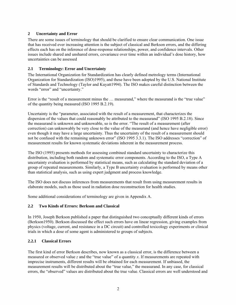
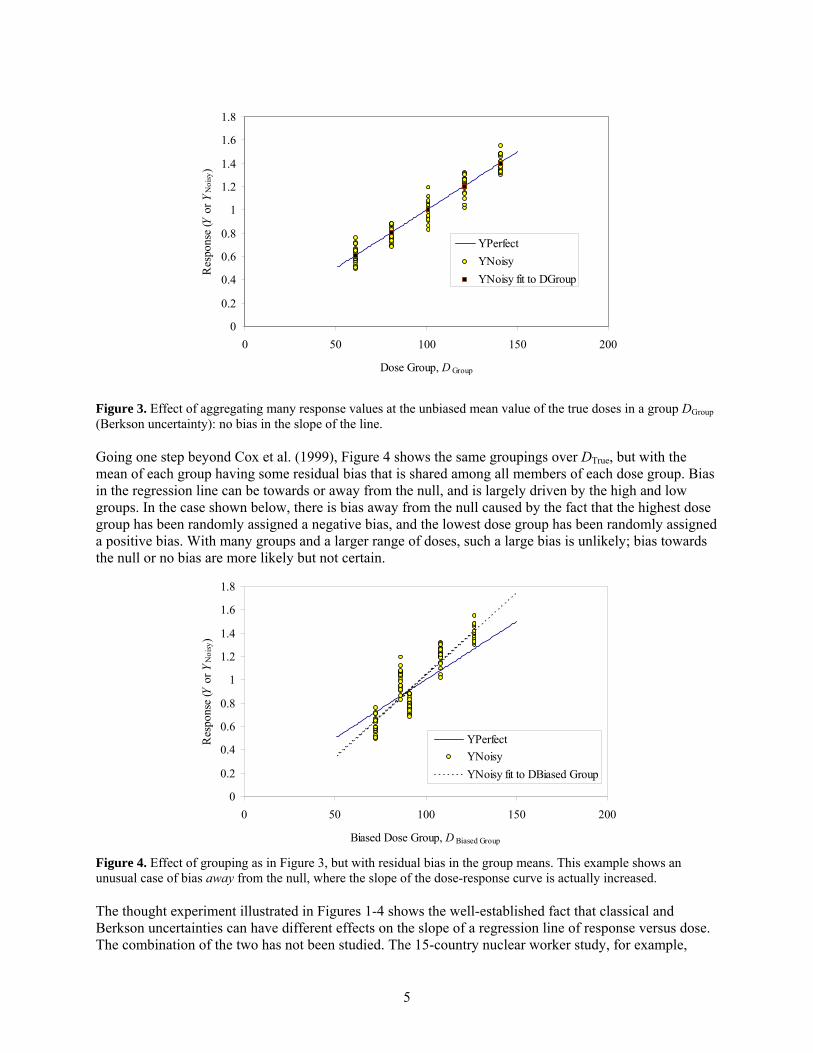
Figure 3. Effect of aggregating many response values at the unbiased mean value of the true doses in a group DGroup (Berkson uncertainty): no bias in the slope of the line. Going one step beyond Cox et al. (1999), Figure 4 shows the same groupings over DTrue, but with the mean of each group having some residual bias that is shared among all members of each dose group. Bias in the regression line can be towards or away from the null, and is largely driven by the high and low groups. In the case shown below, there is bias away from the null caused by the fact that the highest dose group has been randomly assigned a negative bias, and the lowest dose group has been randomly assigned a positive bias. With many groups and a larger range of doses, such a large bias is unlikely; bias towards the null or no bias are more likely but not certain.

Figure 4. Effect of grouping as in Figure 3, but with residual bias in the group means. This example shows an unusual case of bias away from the null, where the slope of the dose-response curve is actually increased. The thought experiment illustrated in Figures 1-4 shows the well-established fact that classical and Berkson uncertainties can have different effects on the slope of a regression line of response versus dose. The combination of the two has not been studied. The 15-country nuclear worker study, for example,

0

0.2

0.4

0.6

0.8

1

1.2

1.4

1.6

1.8

0 50 100 150 200

Biased Dose Group, D Biased Group

Res

pons

e (Y

or Y

Noi

sy)

YPerfectYNoisyYNoisy fit to DBiased Group

0

0.2

0.4

0.6

0.8

1

1.2

1.4

1.6

1.8

0 50 100 150 200

Dose Group, D Group

Res

pons

e (Y

or Y

Noi

sy)

YPerfectYNoisyYNoisy fit to DGroup

6

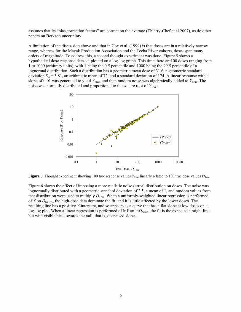
assumes that its “bias correction factors” are correct on the average (Thierry-Chef et al.2007), as do other papers on Berkson uncertainty. A limitation of the discussion above and that in Cox et al. (1999) is that doses are in a relatively narrow range, whereas for the Mayak Production Association and the Techa River cohorts, doses span many orders of magnitude. To address this, a second thought experiment was done. Figure 5 shows a hypothetical dose-response data set plotted on a log-log graph. This time there are100 doses ranging from 1 to 1000 (arbitrary units), with 1 being the 0.5 percentile and 1000 being the 99.5 percentile of a lognormal distribution. Such a distribution has a geometric mean dose of 31.6, a geometric standard deviation SG = 3.81, an arithmetic mean of 72, and a standard deviation of 174. A linear response with a slope of 0.01 was generated to yield YTrue, and then random noise was algebraically added to YTrue. The noise was normally distributed and proportional to the square root of YTrue .

Figure 5. Thought experiment showing 100 true response values YTrue linearly related to 100 true dose values DTrue. Figure 6 shows the effect of imposing a more realistic noise (error) distribution on doses. The noise was lognormally distributed with a geometric standard deviation of 2.5, a mean of 1, and random values from that distribution were used to multiply DTrue. When a uniformly-weighted linear regression is performed of Y on DNoisy,, the high-dose data dominate the fit, and it is little affected by the lower doses. The resulting line has a positive Y-intercept, and so appears as a curve that has a flat slope at low doses on a log-log plot. When a linear regression is performed of lnY on lnDNoisy, the fit is the expected straight line, but with visible bias towards the null, that is, decreased slope.

0.001

0.01

0.1

1

10

100

0.1 1 10 100 1000 10000

True Dose, D True

Res

pons

e (Y

or Y

Noi

sy)

YPerfectYNoisy

7

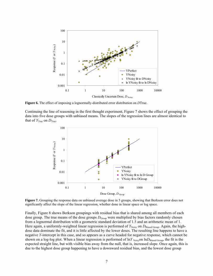
Figure 6. The effect of imposing a lognormally-distributed error distribution on DTrue. Continuing the line of reasoning in the first thought experiment, Figure 7 shows the effect of grouping the data into five dose groups with unbiased means. The slopes of the regression lines are almost identical to that of YTrue on DTrue.

Figure 7. Grouping the response data on unbiased average dose in 5 groups, showing that Berkson error does not significantly affect the slope of the linear regression, whether done in linear space or log space. Finally, Figure 8 shows Berkson groupings with residual bias that is shared among all members of each dose group. The true means of the dose groups DGroup were multiplied by bias factors randomly chosen from a lognormal distribution with a geometric standard deviation of 1.5 and an arithmetic mean of 1. Here again, a uniformly-weighted linear regression is performed of YNoisy on DBiased Group. Again, the high-dose data dominate the fit, and it is little affected by the lower doses. The resulting line happens to have a negative Y-intercept in this case, and so appears as a curve headed for negative response, which cannot be shown on a log-log plot. When a linear regression is performed of lnY Noisyon lnDBiased Group, the fit is the expected straight line, but with visible bias away from the null, that is, increased slope. Once again, this is due to the highest dose group happening to have a downward residual bias, and the lowest dose group

0.001

0.01

0.1

1

10

100

0.1 1 10 100 1000 10000

Classically Uncertain Dose, D Noisy

Res

pons

e (Y

or Y

Noi

sy)

YPerfectYNoisyYNoisy fit to DNoisyln YNoisy fit to ln DNoisy

0.001

0.01

0.1

1

10

100

0.1 1 10 100 1000 10000

Dose Group, D Group

Res

pons

e (Y

or Y

Noi

sy)

YPerfectYNoisyln YNoisy fit to ln D GroupYNoisy fit to DGroup

8

happening to have an upward residual bias. Bias towards the null or no bias are more likely but not certain.

Figure 8. Effect of lognormally-distributed residual bias in the group doses. The two though experiments indicate why it is important to distinguish between classical and Berkson uncertainty.

2.3 Shared and Unshared Errors Stram and Kopecky (2003) identified shared and unshared components of error. Their notation is mostly used here with the exception that D is reserved for “dose” rather than “disease.” For individual i, the true dose DTrue,i is related to the corrected dose DCorr,i by

,A,SA,CorrM,SM,True iiii DD εεεε ++= . 1where εSM is shared multiplicative error, εM,i is unshared multiplicative error, εSA is shared additive error, and εA,i is unshared additive error. They assume that all ε are independent, with Expectation(εSM) = E(εSM) = E(εM,i) = 1 and E(εSA) = E(εA,i) = 0. This means that, on the average, DCorr,i is unbiased. It will be necessary to go beyond this unbiased assumption of Stram and Kopecky (2003), as was shown in the thought experiments above for group doses with residual bias. Thierry-Chef et al. (2007) give “intrinsic sampling variation in measurements inherent to different types of dosimeters, referred to as laboratory error” as an example of “errors that are independent from person to person, and are thus ‘unshared.’ For these errors, the ‘classical error’ model applies, in which the estimated values of the input date are assumed to be distributed around the true values of the input data for each subject.” By contrast, systematic corrections to dosimetry results are needed to remove bias due to over- or under-response due to radiation energy and the geometry of irradiation. Such corrections are intended to “produce corrected doses that are, on average, unbiased estimates of the target dose of interest (e.g. organ doses)” (Thierry-Chef et al.2007). True doses for individual workers “may differ from the doses obtained by applying the group bias factor” and are thus unshared errors. Under the assumption that the “group

0.001

0.01

0.1

1

10

100

0.1 1 10 100 1000 10000

Biased Dose Group, D Biased Group

Res

pons

e (Y

or Y

Noi

sy)

YPerfectYNoisyYNoisy fit to DBiased Groupln YNoisy fit to ln D Biased Group

9

bias factors are estimated without error, the group mean doses (after the application of the bias factor) will be correct, and thus these errors follow a Berkson model.”

2.4 Work on the Techa River Dosimetry System Napier (2007; 2008) has drafted an uncertainty proposal for the Techa River Dosimetry System. For each parameter in the Monte Carlo model, Napier identifies whether it is shared (and if so, among whom), and whether it is classical or Berkson. Much of the approach to reconstructing doses in the Techa River population differs from the approaches needed for the Mayak worker population. To the maximum extent possible, the two approaches should be coordinated and made to match where possible.

2.5 Use of Uncertain Dosimetry Results in Epidemiology Recently, several authors have reported methods for using uncertain dosimetry data in epidemiology (Stayner et al.2007; Li et al.2007). There remain challenges in this area.

10

3 Correction Factors It is necessary to discuss raw dosimetry results and corrections to them. There are measured doses, corrected doses, and “true” doses.

3.1 ISO Definitions The International Organization for Standardization (ISO; 1995) defines an uncorrected result as the result of a measurement before correction for systematic error. A corrected result is the result of a measurement after correction for systematic error. A correction is a value added algebraically to the uncorrected result of a measurement to compensate for systematic error. A correction factor is a numerical factor by which the uncorrected result of a measurement is multiplied to compensate for systematic error.

3.2 Discussion of Previous Approaches to Correcting Dosimetry Results In the paper outlining approaches to managing errors and uncertainties for the “15 Country Study,” Thierry-Chef et al. (2007) define a “bias factor”1 B as

DoseTrue

DoseMeasuredB = . 2

In ISO parlance, the “true dose” is not known or knowable, so “conventionally true dose” would be a better term, and adequate for this discussion:

DoseTrueallyConvention

DoseMeasuredB = . 3

Thierry-Chef et al. assume that each component of bias is lognormally distributed. They explain that “systematic errors (i.e., biases, B) from each source of error were characterized and quantified, as well as the uncertainty (K) on these systematic errors. The interval (B/K, B×K) is the 95% confidence interval on the bias factor. Overall bias factors, B, are obtained by multiplying together individual bias factors:

. ∏=i

iBB ” 4

“If Si is the standard deviation of lnBi and the Bi are independent, then the standard deviation of lnB is estimated by ∑=

i iSS 2 and the overall uncertainty, K, is given by

).96.1exp( SK = ” 5Note that, if the bias is lognormally distributed, K = SG

1.96, where SG is the geometric standard deviation. Thierry-Chef et al. state that “Correction Factors” for converting recorded doses to Hp(10) and organ doses were then derived as the mean of the lognormal distributions, i.e.

.

2exp

2

⎟⎟⎠

⎞⎜⎜⎝

⎛=

SBFactorCorrection ”

6

1 If B is used to correct for systematic error, ISO would call B a correction factor.

11

Thierry-Chef et al. do not explain how such Correction Factors are used. If Eqs. 2 and 3 are correct, then B must be the expectation value (arithmetic mean) of the bias factor. But Eq. 4 is only correct if the Bi are the geometric mean of the various lognormals. Similarly, the statement “The interval (B/K, B×K) is the 95% confidence interval on the bias factor” clearly implies that B is the geometric mean of the bias distribution. If B is the geometric mean, then Correction Factor in Eq. 6 is less than the geometric mean and cannot be the mean. If B is the arithmetic mean, then Eq. 6 specifies that Correction Factor is the geometric mean. Dividing a Measured Dose by such a Correction Factor would produce, “on the average,” a correct “Conventionally True Dose.” Equations 2-6 can only be simultaneously true if S is zero and Eq. 6 is simply Correction Factor = B. In that case, the arithmetic mean of a lognormal distribution is equal to the geometric mean. But since the B values given later in the paper, are not equal to 1, the equations cannot all be correct. This same difficulty, that is, the assumption that the arithmetic mean is equal to the geometric mean for a lognormally-distributed uncertainty, is encountered on page 62 in reference (15) of Thierry-Chef et al., which is the National Research Council book by Masse et al. (1989): “It should be noted that the mean of the lognormal distribution is a factor of exp(S2/2) higher than the median; however, this source of bias is negligible relative to the overall uncertainty and can be safely ignored for most purposes.” The method of Masse et al. (1989) was also used by Daniels and Schubauer-Berigan (2005), but those authors used the method of Fix et al. (2005) in subsequent work (Schubauer-Berigan et al.2007). Masse and co-authors (1989) defined a bias factor, B, as

,Corr

Meas

DD

B = 7

where DMeas is the measured dose and DCorr is the corrected dose2. If DMeas is the result of several simultaneous measurements, it is a weighted or unweighted average of those measurements (ISO 1995). If DMeas is the result of a single measurement, it is taken as the expectation value of repeated measurements of DMeas. This equation is the same as Eq. 2. Because DCorr is to be estimated from DMeas, Eqn. 7 is rearranged to become

.MeasCorr B

DD = 8

This rearrangement results in dividing by the bias factor. When an uncertainty distribution is applied to the bias factor, DMeas is divided by the uncertainty distribution. Dividing by probability distributions is not commonly done because there is no analytical solution for distributions other than the lognormal. It can be shown that there is only one distribution whose reciprocal is the same type of distribution as the original distribution; this is the lognormal. Furthermore, the reciprocal of a lognormal with a geometric mean (median) of 1 is the very same lognormal with the same geometric standard deviation. However, if the mean of the lognormal is taken as 1, then the mean of the reciprocal will not be 1, and using such a distribution in the denominator of an equation injects an unintended additional bias. Thus, dividing by a probability distribution is problematic and is likely to produce counter-intuitive results.

2 Masse et al. (1989) called this the “true value,” but it is really the measured value corrected for bias (systematic error).

12

3.3 Modification of Previous Approach that Doesn’t Assume that the Arithmetic and Geometric Means of a Lognormal Distribution Are Equal

The difficulty of dividing by an asymmetric probability distribution was addressed by Fix et al. (2005) as reported by Scherpelz et al. (2005) and Strom et al. (2005). That method is reproduced here since it has not been widely published. It is shown here that assuming the arithmetic mean and median (geometric mean) are the same for a lognormally-distributed uncertainty is untenable when geometric standard deviations rise above 2, as they do for neutron doses. Fix et al. (2005) developed point estimates of the various components requiring bias correction factors, and used a variety of sources to develop lognormal uncertainty distributions for the various components of bias, such as radiation energy dependence and irradiation geometry dependence. However, the arithmetic mean of each component’s lognormal distribution was set to 1, so that, on average, each component of bias correction was unchanged. When the components were combined by multiplication, the geometric mean (median) of each lognormal distribution was multiplied together to get the geometric mean of the product distribution, and the standard deviations of the natural logarithms of each distribution combined in quadrature to yield the standard deviation of the logs of the product distribution. The solution to the difficulty of dividing by an asymmetric probability distribution is to define a new bias correction factor (formerly bias factor) B' that is the reciprocal of the bias factor in Eqn. 7 to produce a point estimate of the corrected dose:

.MeasMeas

Point Corr, BDB

DD ′⋅== 9

When B' is later multiplied by a probability distribution representing uncertainty, the ordinary properties of uncertainty distributions can be applied. An illustration of this correction and the application of an uncertainty distribution to the correction is shown in Figure 9.

13

Figure 9. Correction of a dose DMeas to a point estimate of dose DCorr, Point by multiplying by a bias correction factor B'. The probability density function of DCorr, Dist is computed by applying a lognormal uncertainty distribution U whose arithmetic mean 1=U . In other words, B' is the arithmetic mean of a lognormal distribution whose geometric mean is less than B' For this work, B' represents the ISO correction factor for systematic error, and is comprised of the product of all multiplicative correction factors:

.1

i

n

iBB ′=′ Π

=

10

Denoting a lognormal distribution as Λ(μ,σ 2), where μ denotes the logarithm of the geometric mean, and σ 2 denotes the square of the logarithm of the geometric standard deviation, it can be shown that the product of two lognormal distributions is lognormal:

( ) ( ) ( )22

2121

222

211 ,,, σσμμσμσμ ++Λ=ΛΛ 11

(Aitchison and Brown 1981). This property permits relatively simple propagation of uncertainties associated with the various bias components B'i, but does not permit the propagation of other kinds of bias components, such as addition of constants. A discussion of the application of this method to the calculation of organ doses from external dosimeter readings is given in the Appendix.

3.4 Asymmetry of Confidence Intervals about the Mean of a Lognormally-Distributed Variable A difficulty in this assumption that uncertainties are lognormally distributed arises from a property of the lognormal distribution that is mentioned by Masse et al. (1989) but assumed to be negligible (Masse et al. 1989, p. 52). When the logarithms of a variable are distributed normally, the central tendency of that distribution is the logarithm of the median (geometric mean), not the expectation value (arithmetic mean) (Aitchison and Brown1981; Strom and Stansbury2000). The value of the parameter that is needed as input to an epidemiology study is the latter, since it is an unbiased estimator of the parameter. For a lognormally distributed variable B', we denote the arithmetic mean by B′ , and the median (geometric mean) by 50B′ . Letting µ denote the average logarithm of the B', and SG denote the geometric standard deviation, we have

),exp(50 μ=′B 12

),exp(sSG = 13

DoseProb

abili

ty D

ensi

tyDMeas

B'

DCorr, Dist = U B' DMeas

DCorr, Point = B' DMeas

14

and

),2/exp( 2sB +=′ μ 14The difficulty is that a measured value is taken to be the expectation value (arithmetic mean) of a variable, namely, B′ , not the geometric mean of a variable, 50B′ . The ratio 50/ BB ′′ , called mean-to-median ratio, is shown in Figure 10 and Table 3.1. Contrary to the claim in the NRC report (1989), the mean-to-median ratio is not negligible for geometric standard deviations (SGs) of 2 or more. For example, in Table 7 of Thierry-Chef et al. (2007), the largest bias and uncertainty values are for Facility-5, 1943-1952, where Bcolon is 2.31 and Kcolon is 1.99. The latter value implies that s = 0.351, with SG = 1.42 and 50/ BB ′′ = 1.064. While this is just over 6% different and not very important, when SG reaches 2, it’s a 27% difference. Thierry-Chef et al. did not have to address neutron doses inferred from neutron-to-gamma ratios, which have substantially larger SG values (Fix et al. 2005). A numerical example using larger SGs is shown in Appendix B.

15

Figure 10. Relationship of s, the natural logarithm of the geometric standard deviation (SG or GSD) and the mean-to-median ratio 50/ BB ′′ to the SG. Table 3.1. Relationship of s, the natural logarithm of the geometric standard deviation (SG) and the mean-to-median ratio 50/ BB ′′ to the SG.

SG s = ln(SG) mean/median = 50/ BB ′′ 1 0 1

1.5 0.41 1.09 2 0.69 1.27

2.5 0.92 1.52 3 1.10 1.83

3.5 1.25 2.19 4 1.39 2.61

4.5 1.50 3.10 5 1.61 3.65

5.5 1.70 4.28 6 1.79 4.98

6.5 1.87 5.77 7 1.95 6.64

0

1

2

3

4

5

6

7

8

0 2 4 6 8

GSD

mea

n/m

edia

n o

r s

smean/median

16

The fact that this correction is not negligible leads to another difficulty. Since we want to use B′ rather than 50B′ we must account for the fact that the 2.5 %ile and 97.5 %ile points on the distribution are not symmetric about B′ , even though they are symmetric about 50B′ . This is illustrated in Figure 11 and Figure 12 for a lognormal uncertainty distribution U with an arithmetic mean of 1 and a SG of 3. These figures illustrate that the 2.5% and 97.5% confidence intervals occur at 1.959963 or ~1.96 geometric standard deviations from the geometric mean (median). These are a factor of

96.1G96.1 SK = 15

above or below the median. For a lognormal distribution with a SG of 3, K1.96 = 8.61. Because of the asymmetry, the confidence intervals about the mean of a lognormal distribution cannot be expressed by a single factor. Two new factors must be introduced. It is seen in Figures 11 and 12 that the 97.5% confidence value for U occurs at a factor

)2/exp( 296.1Mean Above 96.1 sSK G −= 16

above the mean, while the 2.5% confidence value for U occurs at a factor

)2/exp( 296.1Mean Below 96.1 sSK G += 17

below the mean. Note that exp(s2/2) is just the mean-to-median ratio from Table 1. For a lognormal distribution with a SG of 3, K1.96 Above Mean = (8.61)÷(1.828) = 4.71, while K1.96 Below Mean = (8.61)× (1.828) = 15.75.

Figure 11. Probability density function for a lognormally distributed uncertainty distribution U with an arithmetic mean of 1 and a Sg of 3 plotted against U. The 97.5 and 2.5 percentile points are equal to the median (geometric mean) multiplied or divided by K1.96, respectively. However, the same is not true for the mean, which is the value that must be used to avoid biasing B'.

0

0.2

0.4

0.6

0.8

1

1.2

1.4

1.6

0 1 2 3 4 5 6

U

p(U

)

mean = 1

97.5 %ile

mode

2.5 %ile

median

17

Figure 12. Lognormal distribution with an arithmetic mean of 1 and a SG of 3 plotted against the natural logarithm of U, the same distribution plotted in Figure 11. The 97.5 and 2.5 percentile points are equal to the median (geometric mean) multiplied or divided by K1.96, respectively, as shown by their symmetric distribution about the median. However, they are not symmetric about the mean, which is the value that must be used to avoid biasing B'. In what follows, lognormal uncertainty distributions U with arithmetic means of 1 are applied to multiplicative bias factors B', where B' = 1/B. Thus, the mean of B'×U = B', and the confidence limits for B' are

.

and

Mean Above 96.197.5%ile

Mean Below 96.12.5%ile

KBBK

BB

×′=′

′=′

18

0

0.05

0.1

0.15

0.2

0.25

0.3

0.35

0.4

0.45

-5 -4 -3 -2 -1 0 1 2 3 4

ln(U )

p(ln

(U))

mean of lognormal

mean, median, and mode of logs

mode of lognormal

97.5%ile2.5%ile

median of lognormal

18

4 Examples of Contributions to Bias Correction and Uncertainty in Dose Reconstruction There is an extensive body of work on uncertainty in dosimetry and in dose reconstruction, and guidance is currently under development by the U.S. National Council on Radiation Protection and Measurements (NCRP).

4.1 Elements Contributing to Bias and Uncertainty for External Dosimetry Three distinct cases exist for dose reconstruction due to external irradiation: occupational neutrons, occupational photons, and medical exposures.

4.1.1 Neutrons Fix et al. (2005) examined bias and uncertainty in external dosimetry for neutrons, posing 24 questions, as listed in Table 4.1. These questions are sufficiently generic to apply to Mayak.

19

Table 4.1. Topics to be addressed in the external dosimetry of neutrons that give rise to bias corrections and uncertainties. Name Question 1. Unrecorded

Offsite Dose Did an individual receive doses off-site during a given year that either were NOT measured or NOT transferred to the site where employment is?

2. Recorded Offsite Dose

Did an individual receive doses off-site during a given year that were transferred to the site where employment is?

3. Neutron Monitoring

Was there a neutron monitoring program during a given year?

4. Measurement Technology

What instrument or device was used to make measurements for a given subject during a given year?

5. Calibration How was the instrument or device calibrated? 5.1. Is it known what neutron calibration source was used? 5.2. How certain is the primary spectrum of the calibration neutron source? 5.3. How well was the calibration neutron source characterized or

calibrated? 5.4. How well the calibration facility was characterized for primary and

scattered neutrons? 6. Signal Fade How did the signal fade or deteriorate before processing? 7. Reproducibility How consistently was the instrument or measuring device manufactured,

processed and read out? 8. Measurement

Units What units was the measurement recorded in?

9. Conversion Factors

What conversion factors were applied to a measurement result?

10. Workplace Neutron Spectra

What neutron spectrum the worker was exposed to?

11. Representativeness How well did the measurement represent the quantity of interest? 12. Uniformity How uniform was the irradiation field that the worker was exposed to? 13. Radiation Field

Directional Characteristics

What directions the neutrons were coming from (directional properties)?

14. Mixed Radiation Field Response Characteristics

What response did the neutron instrument or measuring device have to other types of radiation and to radioactive contamination?

15. Morphological Similarity

How physically similar was a particular individual to the calculational phantoms used in fluence to dose conversions?

16. Censored Data Were results less than some threshold of detection or less than some threshold for recording censored?

17. Missing data What were the procedures for lost or damaged dosimeters? 18. Dosimeter

Technology What dosimeter technology was employed?

19. Dosimeters Worn Were dosimeters not worn when they were assumed to be worn (e.g., forgotten)?

20. Data Recording Errors

Were there errors in recordkeeping, transcription, keying, or personal identifiers (e.g., name changes, misspellings)?

21. Imputed Dose Uncertainty

What is the uncertainty in imputed doses?

20

For each of these questions, uncertainty distributions and, if needed, bias correction factors, were developed as a function of time, working conditions, and dosimeter technology. Most uncertainty distributions were taken as lognormal, multiplicative distributions. Some uncertainty components were algebraically additive. In cases where doses were imputed, that is, when doses were not based on individual dosimetry results but rather calculated from knowledge of workplace conditions and job titles or coworker measurements, large uncertainties resulted. Information in addition to dosimetry results is needed. For occupational external exposure to neutrons (both low- and high-LET components), consideration is needed of

• Worker, workplace, and geometry considerations o imputation of neutron energy spectrum o imputation of angular exposure distribution by job title (fractions AP, PA, LAT, ROT,

ISO) o imputation of Kn ≡ Dn/Dγ = (“gamma dose”)/(“neutron dose”)

• imputed doses o gamma air absorbed dose/neutron ratios

4.1.2 X- and Gamma Radiation An analogous list of questions, although somewhat shorter, can be posed for external dosimetry for photons (x- and gamma radiation). While bias correction factors have been developed for the Mayak worker study under JCCRER Project 2.4 (Smetanin, Vasilenko, and Scherpelz2007; Smetanin et al.2007; Vasilenko et al.2007d), quantitative expressions of uncertainty for these bias factors haven’t been developed. Information in addition to dosimetry results needed to assess uncertainty. There are a variety of sources of such information. Classical uncertainty will be assessed differently for different exposure/measurement groups for many time periods and dose measurement technologies or inference methods. Project 2.4 personnel expect to begin to work out the details during a meeting in late May and early June 2008. JCCRER Project 2.4 researchers had already catalogued and completed assessment of uncertainty for many aspects of the dosimetry in DOSES-2005 (Vasilenko et al.2007c; Khokhryakov et al.2007; Vasilenko et al.2007a; Vasilenko et al.2007b). Using that notation, additional information should be codified as described below for occupational external photons. Similar approaches are taken for beta, neutron, medical, and internal irradiations. Each approach depends on exposure scenario and year. For occupational external exposures to photons, consideration must be made of the following points:

• Worker, workplace, and geometry considerations o imputation of photon energy spectrum o imputation of angular exposure distribution by job title (fractions AP, PA, LAT, ROT,

ISO) • Air absorbed dose assessment method

o Dγ rec = C’γ rec × Dγ dos = C’γ rec × Cγ dos × Dγ arch, where C’γ rec ≡ 1/Cγ rec as defined in Vasilenko et al. (2007). Convert dosimeter result Dγ arch to air absorbed dose Dγ rec using units conversion factors, photon energy spectrum, angular exposure geometry of dosimeter on worker, and dosimeter response characteristics

IFK IFK+Pb IFKU Pocket ion chambers

21

Offiste dose reports o convert imputed dose result to air absorbed dose using photon energy spectrum, angular

exposure geometry of worker, and dosimeter response characteristics missing values during a monitoring period exposed but unmonitored workers for whom doses are inferred from

measurements on co-workers exposed but unmonitored workers for whom doses are inferred from dose rate

measurements and stay-times exposed but unmonitored workers for whom doses are inferred from process

knowledge and stay-times • Dγ org-i = Cγ org-i × Dγ rec Conversion of air absorbed dose to organ dose

o imputation of photon energy spectrum o imputation of angular exposure distribution by job title o calculation of organ doses

• Uncertainties in Cγ org-i, C’γ rec, and Cγ dos are expressed as lognormal distributions with arithmetic means and geometric standard deviations as described in the Uncertainty Proposal. The values of the arithmetic means and geometric standard deviations are based on analysis of the factors considered above, much of which has already been done. Sensitivity analysis, e.g., Monte Carlo simulation of distributions using different worker and dosimeter exposure geometries, different photon spectra, variability in calibration curves, etc., can inform these choices.

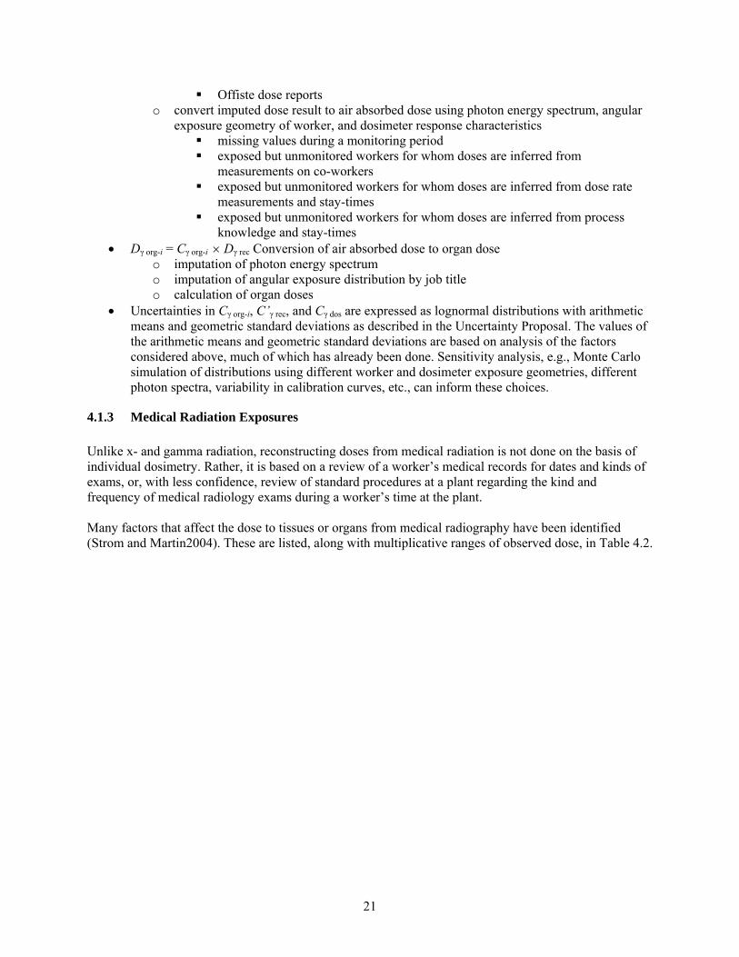
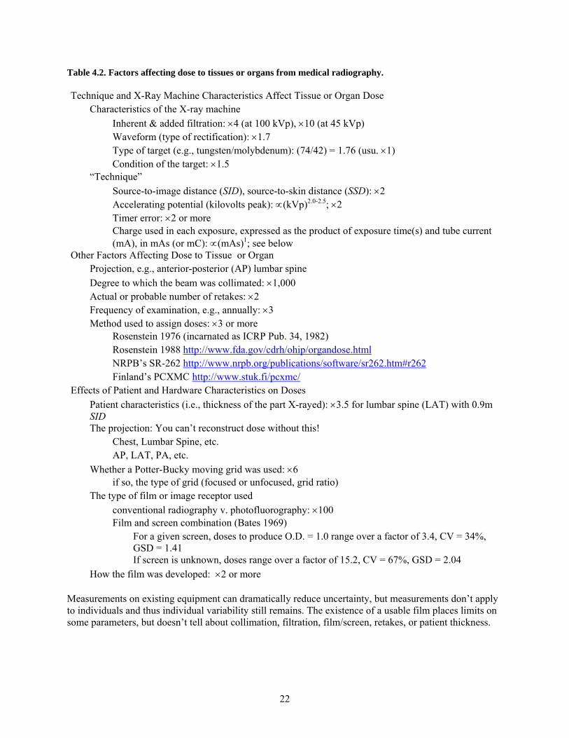
4.1.3 Medical Radiation Exposures Unlike x- and gamma radiation, reconstructing doses from medical radiation is not done on the basis of individual dosimetry. Rather, it is based on a review of a worker’s medical records for dates and kinds of exams, or, with less confidence, review of standard procedures at a plant regarding the kind and frequency of medical radiology exams during a worker’s time at the plant. Many factors that affect the dose to tissues or organs from medical radiography have been identified (Strom and Martin2004). These are listed, along with multiplicative ranges of observed dose, in Table 4.2.

22

Table 4.2. Factors affecting dose to tissues or organs from medical radiography. Technique and X-Ray Machine Characteristics Affect Tissue or Organ Dose

Characteristics of the X-ray machine Inherent & added filtration: ×4 (at 100 kVp), ×10 (at 45 kVp) Waveform (type of rectification): ×1.7 Type of target (e.g., tungsten/molybdenum): (74/42) = 1.76 (usu. ×1) Condition of the target: ×1.5 “Technique” Source-to-image distance (SID), source-to-skin distance (SSD): ×2 Accelerating potential (kilovolts peak): ∝(kVp)2.0-2.5; ×2 Timer error: ×2 or more Charge used in each exposure, expressed as the product of exposure time(s) and tube current

(mA), in mAs (or mC): ∝(mAs)1; see below Other Factors Affecting Dose to Tissue or Organ

Projection, e.g., anterior-posterior (AP) lumbar spine Degree to which the beam was collimated: ×1,000 Actual or probable number of retakes: ×2 Frequency of examination, e.g., annually: ×3 Method used to assign doses: ×3 or more Rosenstein 1976 (incarnated as ICRP Pub. 34, 1982) Rosenstein 1988 http://www.fda.gov/cdrh/ohip/organdose.html NRPB’s SR-262 http://www.nrpb.org/publications/software/sr262.htm#r262 Finland’s PCXMC http://www.stuk.fi/pcxmc/

Effects of Patient and Hardware Characteristics on Doses Patient characteristics (i.e., thickness of the part X-rayed): ×3.5 for lumbar spine (LAT) with 0.9m

SID The projection: You can’t reconstruct dose without this! Chest, Lumbar Spine, etc. AP, LAT, PA, etc. Whether a Potter-Bucky moving grid was used: ×6 if so, the type of grid (focused or unfocused, grid ratio) The type of film or image receptor used conventional radiography v. photofluorography: ×100 Film and screen combination (Bates 1969) For a given screen, doses to produce O.D. = 1.0 range over a factor of 3.4, CV = 34%,

GSD = 1.41 If screen is unknown, doses range over a factor of 15.2, CV = 67%, GSD = 2.04 How the film was developed: ×2 or more

Measurements on existing equipment can dramatically reduce uncertainty, but measurements don’t apply to individuals and thus individual variability still remains. The existence of a usable film places limits on some parameters, but doesn’t tell about collimation, filtration, film/screen, retakes, or patient thickness.

23

4.1.4 Intakes of Radionuclides For doses resulting from intakes of radionuclides, the important factors have been outlined in several recent papers (Bess et al.2007; Etherington et al.2006; Krahenbuhl et al.2005). Bayesian approaches to uncertainty are planned as well (Romanov et al.2007). Classification of uncertainty into shared and unshared components, as well as into classical and Berkson components, probably still remains to be done.

4.2 Residual Systematic Error When bias corrections have been made as well as can be done, given uncertain knowledge of all the variables that contribute to bias, the resulting B' may differ systematically from the value B'True that would yield DTrue:

MeasResidMeasTrueTrue DBBDBD ′′=′= 19The residual bias is shared by those individuals for whom it applies, but not by others. Residual, uncorrected bias is likely to differ for differing job titles, different work locations, and different years (e.g., as shielding or ventilation was installed to lower doses and intakes, work practices evolved to reduce doses, personal protective equipment introduced, etc.). Residual uncorrected bias is not discussed in any analyses of Berkson errors known to this author. Current authors are likely to state, “…if the group bias factors are estimated without error, the group mean doses (after application of the bias factor) will be correct, and thus these errors follow a ‘Berkson’ error model” (Thierry-Chef et al. 2007, referencing Schafer and Gilbert 2006), but not address what happens if there are residual errors in the “bias factors.” The fact that the residual uncorrected bias is unknown leads to a need to estimate its magnitude, which must be done by a Type B uncertainty analysis.

4.3 Error, Variability, and Uncertainty It is clear that variability in characteristics of individuals, such as height, weight, metabolism, diet, lifestyle, work habits, and behaviors lead to individual differences from group means. If the true, unbiased group mean is known, then one can label these differences “errors” in the ISO sense of a difference between a measurand and a corrected measurement value. From the perspective of dose reconstruction for health effects research, such differences must be estimated and recorded as uncertainties.

24

5 Intra-individual Covariance of Annual Doses over Time André Bouville recently shared his “Rules for Dosimetry for Epidemiology,” which include “cooperate with the epidemiologists, calculate the annual absorbed dose to the organ of interest, give preference to measurements on individual subjects, ask the right questions during interviews, validate data and doses to eliminate bias, and estimate uncertainties as well as possible” (Strom2007). Often health effects studies do require annual organ doses. For the case of intakes of radionuclides that are tenaciously retained in the body, such as plutonium, americium, and strontium, uncertainties in corrected annual doses will be very highly correlated. The uncertainty of the sum of such annual doses, that is, corrected dose cumulated to some specified date, must be calculated with this covariance in mind. Likewise, uncertainties in corrected annual external dosimetry results for individuals will show some correlation over time for each individual. The uncertainty of the sum of such annual doses, that is, corrected dose cumulated to some specified date, must also be calculated with this covariance in mind.

25

6 A Proposal for a Numerical Expression of Uncertainty in Results of Dose Reconstruction to Be Applied Throughout JCCRER Project 2.4

It is proposed that, for each individual i, each corrected annual dose in year y to a tissue or organ T, DCorr,C,T(i,y) be accompanied by expressions of uncertainty that are divided into classical and Berkson components, and that covariance among components of dose over an individual’s lifetime be included in the assessment of uncertainty in lifetime dose. Measurements on individual subjects include film badge results, bioassay results, and autopsy data. Each of these has associated measurement uncertainty that is a combination of random and systematic uncertainties. The uncertainties will be treated as a combined standard uncertainty following the ISO procedure (ISO 1995). Groups of individuals have corrected doses that are calculated by application of the same bias correction factors. All members in such groups share the uncertainty in those factors, including the residual uncorrected bias. True doses to individuals in the group may differ systematically from the bias corrected doses. Such Berkson errors become uncertainties when the dose is assigned to individuals.

6.1 Specific Proposal for DOSES2008: The Dose-Uncertainty Vector For each individual i, each corrected annual dose (in dose category C) in year y to a tissue or organ T, the corrected dose DCorr,C,T(i,y) will have 5-part numerical expression of uncertainty. The combination of these variables is called a dose-uncertainty vector.

6.1.1 Six Dose Categories For DOSES2008, it is proposed that separate files of DCorr,C,T(i,y) be created and maintained for 1) low-LET gamma external occupational doses; 2) low-LET beta external occupational doses; 3) low-LET (neutron) external occupational doses; 4) high-LET (neutron) external occupational doses; 5) internal occupational doses; and 6) medical doses.

6.1.2 Component 1: The Corrected Annual Dose DCorr,C,T(i,y) The dose value itself is the best corrected dose estimate, that is, the expectation value of the true dose given all that is known about the individual, the measurements on that individual, the workplace, and the measurements made in the workplace. The value recorded for DCorr is not a geometric mean, but an arithmetic mean. Work to create DCorr,C,T(i,y) values is well underway for all 5 categories of dose.

6.1.3 Component 2: The Magnitude of the Uncertainty, SG For reasons described in Sections 3.3 and 3.4, the uncertainty is a lognormal distribution with an arithmetic mean of 1 and a geometric standard deviation SG determined as outlined below.

6.1.4 Component 3: Apportionment of the Variance in Dose Uncertainty, fClassical The variance of this lognormal distribution is

26

( )

.2/),(ln

and )ln where,1

2Corr,

2 22

σ

σσμ

+=

=−= +

yiDμ

(SσeeVar

T

G 20

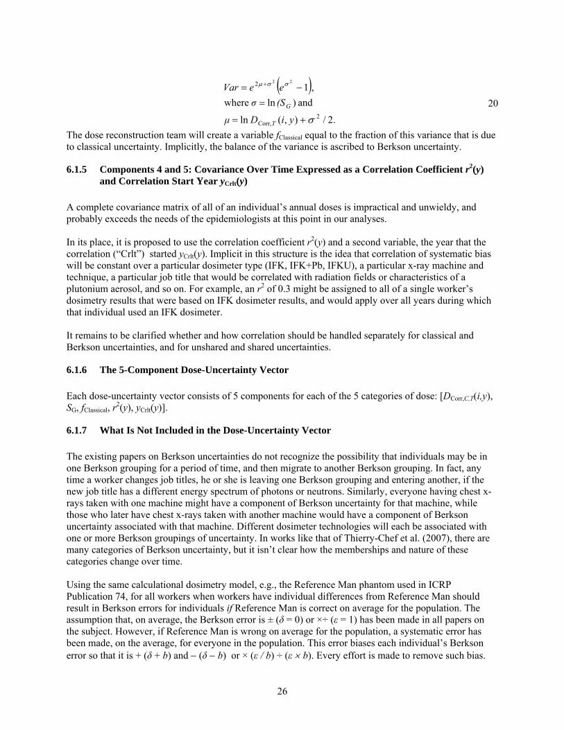
The dose reconstruction team will create a variable fClassical equal to the fraction of this variance that is due to classical uncertainty. Implicitly, the balance of the variance is ascribed to Berkson uncertainty.

6.1.5 Components 4 and 5: Covariance Over Time Expressed as a Correlation Coefficient r2(y) and Correlation Start Year yCrlt(y)

A complete covariance matrix of all of an individual’s annual doses is impractical and unwieldy, and probably exceeds the needs of the epidemiologists at this point in our analyses. In its place, it is proposed to use the correlation coefficient r2(y) and a second variable, the year that the correlation (“Crlt”) started yCrlt(y). Implicit in this structure is the idea that correlation of systematic bias will be constant over a particular dosimeter type (IFK, IFK+Pb, IFKU), a particular x-ray machine and technique, a particular job title that would be correlated with radiation fields or characteristics of a plutonium aerosol, and so on. For example, an r2 of 0.3 might be assigned to all of a single worker’s dosimetry results that were based on IFK dosimeter results, and would apply over all years during which that individual used an IFK dosimeter. It remains to be clarified whether and how correlation should be handled separately for classical and Berkson uncertainties, and for unshared and shared uncertainties.

6.1.6 The 5-Component Dose-Uncertainty Vector Each dose-uncertainty vector consists of 5 components for each of the 5 categories of dose: [DCorr,C,T(i,y), SG, fClassical, r2(y), yCrlt(y)].

6.1.7 What Is Not Included in the Dose-Uncertainty Vector The existing papers on Berkson uncertainties do not recognize the possibility that individuals may be in one Berkson grouping for a period of time, and then migrate to another Berkson grouping. In fact, any time a worker changes job titles, he or she is leaving one Berkson grouping and entering another, if the new job title has a different energy spectrum of photons or neutrons. Similarly, everyone having chest x-rays taken with one machine might have a component of Berkson uncertainty for that machine, while those who later have chest x-rays taken with another machine would have a component of Berkson uncertainty associated with that machine. Different dosimeter technologies will each be associated with one or more Berkson groupings of uncertainty. In works like that of Thierry-Chef et al. (2007), there are many categories of Berkson uncertainty, but it isn’t clear how the memberships and nature of these categories change over time. Using the same calculational dosimetry model, e.g., the Reference Man phantom used in ICRP Publication 74, for all workers when workers have individual differences from Reference Man should result in Berkson errors for individuals if Reference Man is correct on average for the population. The assumption that, on average, the Berkson error is ± (δ = 0) or ×÷ (ε = 1) has been made in all papers on the subject. However, if Reference Man is wrong on average for the population, a systematic error has been made, on the average, for everyone in the population. This error biases each individual’s Berkson error so that it is + (δ + b) and − (δ − b) or × (ε / b) ÷ (ε × b). Every effort is made to remove such bias.

27

How one would assess residual bias that cannot be assessed or removed is unknown. If one can assess it, one removes it. If one cannot assess it, then it’s anyone’s guess how large it may be. Thus, the questions of “With whom is a particular Berkson grouping shared?” and “For how long is a particular Berkson grouping shared?” are not included in the dose-uncertainty vector proposed here. This may be a critical flaw, but developing a method to create and store this kind of information is a completely intractable problem at this point in the project. It could be true that, if Berkson groupings have few individuals, and the individuals change fairly often, that the effect of Berkson groupings on the dose-response relationship and its confidence intervals will have to be reevaluated. Re-evaluation may be needed if individuals often change Berkson groups, and only small proportions of the population are in any single Berkson group at one time. It is unclear whether Berkson errors in this case would have the same effect as classical uncertainties. The rationale for this supposition comes from a thought experiment in which an extreme situation results in the total membership of each Berkson group being 1 individual. The transition from everyone being in a Berkson group to having several Berkson groups to having many Berkson groups to having a different Berkson “group” for each individual (i.e., no two individuals in the same group) would seem to make the distinction between Berkson and classical uncertainties disappear. Furthermore, even with Berkson groups with several or even many members, if individuals move in and out of the groups, it may be difficult to see the same effect. Specifically, for Mayak workers, an individual would be a member of one Berkson group based on job title, another based on work location, a third based on dosimeter type, a fourth based on the years during which various radiation protection measures were or were not present in his or her work location (i.e., shielding or containment or ventilation may have been introduced in one area sooner than in another area). To the extent that individuals changed job titles, membership would shift to some different Berkson groups. Finally, the currently proposed dose-uncertainty vector does not adequately deal with the possibility of zero or negative doses. This is discussed in Appendix C.

6.2 Determining the Uncertainty Parameters of the Dose-Uncertainty Vector Due to limitations on time, resources, knowledge, and the utility of this approach to the epidemiologists, it is proposed that an expert-elicitation process be used to determine SG, fClassical, r2(y), yCrlt(y) for DOSES2008. Refinements of this process must await future funding. The expert-elicitation process will include discussions during meetings, exchanges of electronic mail, and telephone communications. The process will consider all previous work on uncertainties in doses for radiation health studies, with particular emphasis on products of Project 2.4 such as Krahenbuhl et al. (2005) and Zharov et al. (Zharov et al.2007). It is envisioned that the dose-uncertainty vectors may be fairly simple for DOSES2008, with categories for various times and conditions. A conceptual idea of the uncertainty portion of the dose-uncertainty vectors can be seen in Table 3

28

Table 3. Possible dose-uncertainty vectors with placeholder values. The DCorr,C,T(i,y) value is omitted, since it varies for individuals and years. This table is a very rough draft with sample values only. It is not intended to reflect historical values. Exp. Type Exposure Scenario years T SG fClassical r2(y) yCrlt(y) Ext. Low IFK – Workplace No. 1 49-53 all 1.9 0.5 0.2 1949 Ext. Low IFK – Workplace No. 2 49-53 all 2.1 0.5 0.2 1949 Ext. Low IFK+Pb – Workplace No. 1 54-62 all 1.7 0.5 0.2 1954 Ext. Low IFK+Pb – Workplace No. 2 54-62 all 1.8 0.5 0.2 1954 Ext. Low … Ext. High IFK – Workplace No. 1 49-53 all 3.5 0.4 0.3 1949 Ext. High … Med. Chest film 48-60 lung 1.4 0.3 0.3 1948 Med. Chest film 48-60 RBM 3 0.6 0.3 1948 Med. … Int. Chemical Plant, with autopsy data 49-58 lung 2 0.7 0.95 1949 Int. Chemical Plant, with autopsy data 49-58 liver 2 0.7 0.95 1949 Int. Chemical Plant, with autopsy data 49-58 BS 2 0.7 0.95 1949 Int. Chemical Plant, bioassay data only 49-58 lung 3 0.7 0.95 1949 Int. Chemical Plant, bioassay data only 49-58 liver 3 0.7 0.95 1949 Int. Chemical Plant, bioassay data only 49-58 BS 3 0.7 0.95 1949 Int. … Table 3 is a very rough draft with sample values only. It is not intended to reflect historical values.

6.3 Use of the Dose-Uncertainty Vector The existence of a unique dose-uncertainty vector for each annual tissue or organ dose, in the 3 categories of external occupational, internal occupational and medical doses, provides new opportunities for biostatisticians and epidemiologists.

6.3.1 Cumulating Organ or Tissue Doses Up to a Certain Year The dose-uncertainty vectors for each of the 4 dose categories permits analysts to

• add doses up to a certain year, such as 5 or 10 years before the diagnosis of a cancer • create an numerical expression of the uncertainty of that dose • determine the fraction of the variance in the dose that is due to classical and Berkson uncertainty • know that uncertainty correlation over years has been adequately accounted for

6.3.2 Uncertainty Propagation for Cumulated Organ or Tissue Doses Explicit algorithms will be developed by the Project 2.4 team in cooperation with Project 1.1 and our customers, the epidemiologists and biostatisticians. Such algorithms will result in a cumulated dose-uncertainty vector for each of the 4 categories of dose, but without r2(y) and yCrlt(y) since these will have been used to develop the SG and fClassical values.

6.4 Proposed Milestones for the Uncertainty Task Proposed milestones for the uncertainty task are given in Table 4.

29

Table 4. Proposed milestones for the uncertainty task. TBD, to be determined. Number Date Milestone Who U1 TBD Reach agreement on Uncertainty Structure for

future dosimetry databases US Researchers (Projects 2.4 and 1.1), DOE Staff, RF Researchers including epdiemiologists and biostatisticians

U2 TBD Finalize list of “Exposure Scenarios” in in Table “Dose-uncertainty vectors with placeholder values”

US Researchers (Project 2.4), DOE Staff, RF Researchers (Dosimetrists at MPA and SUBI)

U3 TBD Draft detailed criteria and methods for imputing or calculating the values of the dose-uncertainty vector for each “Exposure Scenario;” Implement discussion and training program for all of us on Berkson versus classical uncertainties and implement quality assurance program for Berkson/classical decisions

“

U4 TBD Finalize criteria and methods for calculating the dose-uncertainty vector for each “Exposure Scenario”

“

U5 TBD Complete dose-uncertainty vectors for DOSES2008

“

U6 TBD Submit uncertainty manuscript to scientific journal

“

6.5 Level of Effort A draft level of effort proposal appears in Table 5. Table 5. Draft Level of Effort. TBD = to be determined

JCCRER Project Name Level of Effort, % of Full-Time Equivalent (% FTE)

2.4, Mayak Worker Dosimetry Strom 35 2.4, Mayak Worker Dosimetry Scherpelz 20 2.4, Mayak Worker Dosimetry Krahenbuhl TBD 2.4, Mayak Worker Dosimetry Miller TBD 2.4, Mayak Worker Dosimetry MPA TBD 2.4, Mayak Worker Dosimetry SUBI TBD 2.2, Mayak Worker Epidemiology Gilbert <5 2.2, Mayak Worker Epidemiology SUBI TBD 1.1, Techa River Population Dosimetry Napier <5 1.1, Techa River Population Dosimetry Anspaugh <5 1.1, Techa River Population Dosimetry URCRM TBD 1.2b, Techa River Population Morbidity Davis TBD 1.2b, Techa River Population Morbidity URCRM TBD

30

7 Acknowledgements The author is grateful for critical review and comments from Peter Jacob, Reinhard Mechbach, Bruce A. Napier, Joel L. Rabovsky, Robert I Scherpelz, Evgeny K. Vasilenko, and Peter Zharov. Dale L. Preston and Elaine Ron provided helpful discussion and resources.

31

8 Appendix A: Terminology There are numerous issues regarding terminology that is used differently in different disciplines. For dosimetry, some of the issues to be sorted out are shown in Table 6. Table 6. Dosimetry terms and issues to be discussed and agreed on.

On the one hand… On the other hand… measurand corrected measurement result true dose calculated dose

estimated dose imputed dose modeled dose observed dose reconstructed dose

variability uncertainty error uncertainty classical Berkson shared (across individuals) unshared bias systematic error

precision random error

independence correlation Sometimes the word “error” is used when “uncertainty” is intended, at least in the ISO GUM meaning of “uncertainty” (International Organization for Standardization (ISO)1995). There is concern about shared versus unshared uncertainty, about Berkson versus classical uncertainty. Careful attention must be given to the correct usage of these terms both in English and in Russian.

32

9 Appendix B: Propagation of Uncertainty for Lognormally-Distributed Correction Factors In studies of the health effects of ionizing radiation, it is often necessary to remove bias in the dose variable by correcting dosimetry measurements. When such corrections are lognormally distributed and multiplicative, as in Thierry-Chef et al. (2007) or Masse et al. (1989), care must be used in propagating uncertainty. This paper presents an argument that correction factors are the arithmetic means of lognormal distributions. Any other interpretation, such as the reasoning following Eq. (11) in Schafer and Gilbert (2006), results in biased corrected dose values. Note that in this presentation of the problem, corrected dose values are products of correction factors and measured doses, while in Thierry-Chef et al. (2007) or Masse et al. (1989), one must divide by correction factors. Dividing by probability distributions is less intuitive than multiplying by them, and leads to difficulties if they have any nonzero probability at zero or negative numbers.

9.1 Point Estimates Consider a dosimeter such as a simple film badge that produces a reading DMeas which is a reasonably accurate dose to a dosimeter that is calibrated with a particular energy spectrum of gamma radiation in a particular irradiation geometry, e.g., normal to the dosimeter. Suppose A is a correction for energy response of the dosimeter for anterior-posterior (AP) irradiation so that the product ADMeas is the correct dose to air for AP irradiation in the energy spectrum of gamma radiation to which the worker was exposed, as opposed to the energy spectrum of the calibration radiation. Suppose B is a correction for the angular response of the dosimeter at that energy for the irradiation geometry in which it was believed to have been exposed (e.g., 50% AP and 50% rotational), so that the product ABDMeas is the air dose corrected for angular response. Suppose C is a correction from air dose to tissue or organ dose so that the product ABCDMeas is the correct tissue or organ dose. Suppose one wants to apply correction factors A, B, and C to a measured dose DMeas in such a way that, on the average, DCorr will be unbiased. If one does a deterministic calculation,

MeasCorr DCBAD ⋅⋅⋅= 21the corrected dose is a simple product. Now suppose that one wants to require that the intermediate doses each be correct on the average:

MeasOrgan AngleEnergy Corr

MeasAngleEnergy Corr

MeasEnergyCorr

DCBAD

DBAD

DAD

⋅⋅⋅=

⋅⋅=

⋅=

. 22

This seems simple enough if A, B, and C are point estimates. Suppose that DMeas has a value of 1, and that A, B, and C are 3, 2, and 4, respectively. Then DCorr Energy = 1 × 3 = 3, DCorr Energy Angle = 1 × 3 × 2 = 6, and DCorr Energy Angle Organ = 1 × 3 × 2 × 4 = 24.

33

9.2 Normally-Distributed Correction Factors Now suppose that A, B, and C are uncertain, and are normally distributed. If the point estimate values of A, B, and C are used as the means of the normal distributions, and, say, each has a coefficient of variation (relative standard deviation) of 0.2 so that negative values are highly unlikely, then each of the values DCorr Energy, DCorr Energy Angle, and DCorr Energy Angle Organ will be unbiased on the average, with values of 3, 6 and 24 as in the point estimate example.

9.3 Lognormally-Distributed Correction Factors Now suppose that A, B, and C are uncertain, and are lognormally distributed. Further, suppose that they have geometric standard deviations SG of 3, 2, and 4, respectively. If the point estimate value of A, namely, 3, is used as the geometric mean of a lognormal distribution, then DCorr Energy will have an average value of 3.81, not 3. If instead the point estimate value of A is used as the arithmetic mean of a lognormal distribution, then DCorr Energy will have the correct average value of 3. That is, the geometric mean of the lognormal distribution of A is 2.35, not 3. If the point estimate values of A and B, namely, 3 and 2, are used as the geometric means of lognormal distributions, then DCorr Energy Angle will have an average value of 13.9, not 3 × 2 = 6. If the point estimate values of A and B are used as the arithmetic means of lognormal distributions, then DCorr Energy Angle will have the correct average value of 6. The result is that the geometric mean of the lognormal distribution of A is 2.35, not 3, and the geometric mean of the lognormal distribution of B is 1.094, not 2. If the point estimate values of A, B and C, namely, 3, 2, and 4, are used as the geometric means of lognormal distributions, then DCorr Energy Angle Organ will have an average value of 146, not 3 × 2× 4 = 24. If the point estimate values of A, B and C are used as the arithmetic means of lognormal distributions, then DCorr Energy Angle Organ will have the correct average value of 24. This means that the geometric mean of the lognormal distribution of A is 2.35, not 3, and the geometric mean of the lognormal distribution of B is 1.094, not 2, and the geometric mean of the lognormal distribution of C is 1.53, not 4. The results for these four thought experiments are found in Table 7.

9.4 General Procedure for Propagating Lognormally Distributed Uncertainties If multiplicative correction factors Ai are unbiased, on the average, and are found to be lognormally distributed, then the correct propagation of uncertainty is to find the lognormal distribution whose arithmetic mean iA is equal to the correction factor. The parameters of this lognormal distribution are the geometric mean AGM,i and geometric standard deviation SG,i. The former is

2/)(lnGM,

2G,e iS

ii AA −= . 23The geometric mean of the lognormal distribution of the product of the multiplicative correction factors is

∏=i

iAA GM,overall GM, , 24

while its geometric standard deviation is

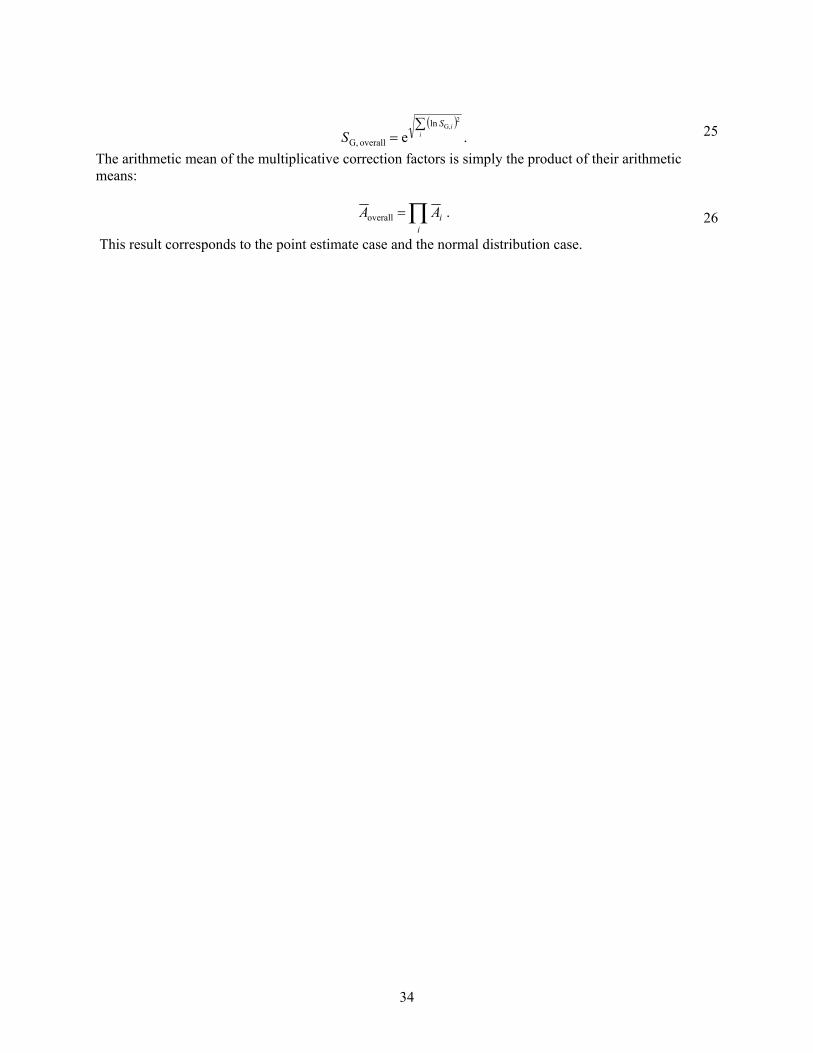
34

( )∑= i

iS

S2

G,ln

overall G, e . 25

The arithmetic mean of the multiplicative correction factors is simply the product of their arithmetic means:

∏=i

iAAoverall . 26

This result corresponds to the point estimate case and the normal distribution case.

35

Table 7. Results of four thought experiments regarding the propagation of uncertainty when multiplying correction factors. In the point estimate and normal distribution cases, values are simply multiplied, and the question of whether they are arithmetic mean (average values or expectation values) or geometric mean (or median) values never arises. In the lognormal case, use of the point estimate values as geometric means (first “lognormal” row) alters the average result of the corrected dose value. A bar denotes an arithmetic mean; SD, standard deviation; GM, geometric mean; SG, geometric standard deviation; DMeas, result of dose measurement; DCorr, corrected dose value.

Energy Correction Factor

Angle Correction Factor

Organ Correction Factor DCorr Energy DCorr Energy Angle

DCorr Energy Angle

Organ

Uncertainty Distribution SD

A, AGM, SG SD

B , BGM SG SD

C , CGM, SG DMeas

Mean, SD

GM, SG

Mean, SD

GM, SG

Mean, SD

GM, SG

Point Estimate

3 -

3 -

2 -

2 -

4 -

4 - 1 3

- 3 -

6 -

6 -

24 -

24 -

Normal Distribution

3 0.6

3 -

2 0.4

2 -

4 0.8

4 - 1 3

0.6 3 -

6 0.72

6 -

24 1.08

24 -

Lognormal Distribution

3.81 2.35

3 2

3.66 8.57

2 3

10.5 61.0

4 4 1 3.81

2.35 3 2

13.9 61.5

6 3.67

145.9 5242

24 6.68

Lognormal Distribution

3 1.85

2.36 2

2 4.69

1.09 3

4 23.3

1.53 4 1 3

1.85 2.36

2 6

26.4 2.58 3.67

24 862

3.95 6.68

36

10 Appendix C: Results that Are Small Compared to Measurement Uncertainty Under some circumstances, it may be necessary to admit the possibility that an uncertain dose may be zero. Under other circumstances, such as a low value of a bioassay measurement, there is a relatively large measurement uncertainty that includes zero and negative values. In these circumstances, a purely lognormal expression for uncertainty is inadequate. While neither a negative dose nor a negative activity has physical meaning, the difference between two doses or the difference between two activities can meaningfully be negative. An individual who receives a series of doses that are small compared to the measurement uncertainty can legitimately have a record of small positive and small negative results. If some components of uncertainty are lognormally distributed and combined as described above, and a component of uncertainty corresponding to measurement error that is normally distributed with a mean of 0, then the resulting distribution may be a sum of a normal distribution and a lognormal distribution. Consider the case of DCorr Energy Angle Organ = 24, as in Appendix B. If, in addition to the correction factors A, B, and C, suppose the original DMeas = 1 was characterized by a normal distribution with a mean of 0 and a standard deviation of 2 as shown in Figure 13. Admittedly, this is a case in which DMeas would be regarded by many as not significantly different from 0, but it illustrates the problem well. Also, the geometric standard deviation of the correction factors is larger than is likely for most kinds of measurements, but it is chosen to illustrate an extreme case. In this example, the normal uncertainty is a classical uncertainty, and the correction factor uncertainty is almost entirely a Berkson uncertainty. Of course, a negative dose is not physically meaningful3. However, setting spurious negative doses to zero without equally compensating for equally spurious positive doses injects a positive bias into sums or averages of doses. Unlike the distribution of the product of lognormal distributions discussed in the main text and in Appendix B, the result of convolving the normal and lognormal distributions is a hybrid distribution that has no known analytical expression. One may wish for example to compute an annual dose from a series of monthly dosimeter results. If one adds doses with such hybrid uncertainty distributions, the classical measurement uncertainties will tend to cancel out, since the classical uncertainties are expected to be independent. The Berkson uncertainties will not diminish with addition.

3 Of course, a negative dose is meaningful if it is the differnce of two positive doses.

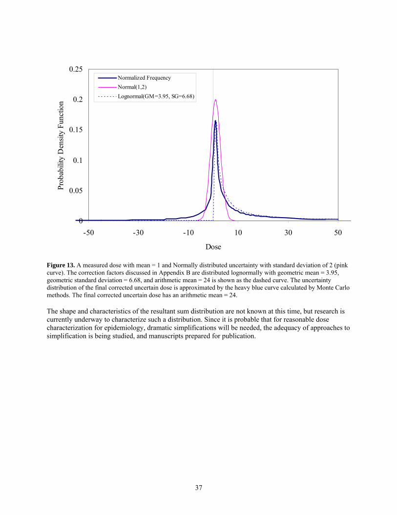
37

0

0.05

0.1

0.15

0.2

0.25

-50 -30 -10 10 30 50

Dose

Prob

abili

ty D

ensit

y Fu

nctio

n

Normalized FrequencyNormal(1,2)Lognormal(GM=3.95, SG=6.68)

Figure 13. A measured dose with mean = 1 and Normally distributed uncertainty with standard deviation of 2 (pink curve). The correction factors discussed in Appendix B are distributed lognormally with geometric mean = 3.95, geometric standard deviation = 6.68, and arithmetic mean = 24 is shown as the dashed curve. The uncertainty distribution of the final corrected uncertain dose is approximated by the heavy blue curve calculated by Monte Carlo methods. The final corrected uncertain dose has an arithmetic mean = 24. The shape and characteristics of the resultant sum distribution are not known at this time, but research is currently underway to characterize such a distribution. Since it is probable that for reasonable dose characterization for epidemiology, dramatic simplifications will be needed, the adequacy of approaches to simplification is being studied, and manuscripts prepared for publication.

38

11 References

Aitchison J and JAC Brown. 1981. The Lognormal Distribution. Cambridge University Press, Cambridge.

Armstrong BG. 1990. "The effects of measurement errors on relative risk regressions." Am.J Epidemiol. 132(6):1176-1184.

Armstrong BG. 1998. "Effect of measurement error on epidemiological studies of environmental and occupational exposures." Occup.Environ Med. 55(10):651-656.

Berkson J. 1950. "Are There 2 Regressions." Journal of the American Statistical Association 45(250):164-180.

Bess JD, MP Krahenbuhl, SC Miller, DM Slaughter, VV Khokhryakov, VF Khokhryakov, KG Suslova, and VV Vostrotin. 2007. "Uncertainties Analysis for the Plutonium Dosimetry Model, DOSES-2005, Using Mayak Bioassay Data." Health Phys 93(3):207-219.

Cox DR, SC Darby, GK Reeves, and E Whitley. 1999. "The Effects of Measurement Errors with Particular Reference to a Study of Exposure to Residential Radon." in Uncertainties in Radiation Dosimetry and Their Impact on Dose-Response Analyses. Publication 99-4541. http://bidug.pnl.gov/references/Ron1999_Uncertainty_Dosimetry.pdf, eds. E Ron and FO Hoffman, National Cancer Institute, Bethesda, Maryland.

Daniels RD and MK Schubauer-Berigan. 2005. "Bias and uncertainty of penetrating photon dose measured by film dosemeters in an epidemiological study of US nuclear workers." Radiat Prot Dosimetry 113(3):275-289.

Etherington G, A Birchall, M Puncher, A Molokanov, and E Blanchardon. 2006. "Uncertainties in doses from intakes of radionuclides assessed from monitoring measurements." Radiat.Prot.Dosimetry. 121(1):40-51.

Fix JJ, RI Scherpelz, DJ Strom, and RJ Traub. 2005. Dose Validation for NIOSH/HERB Multi-Site Leukemia Case Control Study. PNWD-3538, Battelle-Pacific Northwest Division, Richland, Washington.

International Commission on Radiological Protection (ICRP). 1996. "Conversion Coefficients for Use in Radiological Protection Against External Radiation. ICRP Publication No. 74." Ann ICRP 26(3-4).

International Organization for Standardization (ISO). 1995. Guide to the Expression of Uncertainty in Measurement. Corrected and Reprinted, 1995. International Organization for Standardization, Geneva.

Khokhryakov VF, VV Khokhryakov, NA Koshurnikova, NS Shilnikova, PV Okatenko, VV Kreslov, MG Bolotnikova, ME Sokolnikov, KG Suslova, SA Romanov, EK Vasilenko, SC Miller, MP Krahenbuhl, KF Eckerman, and ES Gilbert. 2007. "Mayak Worker Study Project 2.4. Volume III: Internal Dosimetry Dose Reconstruction Methods Used in Preparation of Doses-2005 Database." Health Phys 93(3):CD Supplement.

39

Khokhryakov VF, KG Suslova, VV Vostrotin, SA Romanov, KF Eckerman, MP Krahenbuhl, and SC Miller. 2005. "Adaptation of the ICRP publication 66 respiratory tract model to data on plutonium biokinetics for Mayak workers." Health Phys 88(2):125-132.

Kim HM, Y Yasui, and I Burstyn. 2006. "Attenuation in risk estimates in logistic and Cox proportional-hazards models due to group-based exposure assessment strategy." Ann Occup.Hyg. 50(6):623-635.

Krahenbuhl MP, JD Bess, JL Wilde, VV Vostrotin, KG Suslova, VF Khokhryakov, DM Slaughter, and SC Miller. 2005. "Uncertainties analysis of doses resulting from chronic inhalation of plutonium at the Mayak production association." Health Phys 89(1):33-45.

Küchenhoff H, R Bender, and I Langner. 2007. "Effect of Berkson measurement error on parameter estimates in Cox regression models." Lifetime.Data Anal. 13(2):261-272.

Li Y, A Guolo, FO Hoffman, and RJ Carroll. 2007. "Shared Uncertainty in Measurement Error Problems, with Application to Nevada Test Site Fallout Data." Biometrics 63:1226-1236.

Mallick B, FO Hoffman, and RJ Carrol. 2002. "Semiparametric regression modeling with mixtures of Berkson and classical error, with application to fallout from the Nevada test site." Biometrics 58(1):13-20.

Masse FX, WL Brown, J Areen, WJ Brady, JR Frazier, ES Gilbert, RO Gorson, NA Greenhouse, RL Kathern, NC Rasmussen, and RC Yoder. 1989. Film Badge Dosimetry in Atmospheric Nuclear Tests. National Academy Press, Washington, D.C.

Napier BA. 2008. Assessment of Various Types of Uncertainty in the Techa River Dosimetry System. JCCRER Project 1.1 Unscheduled Report, Pacific Northwest National Laboratory, Richland, Washington.

Napier BA. 2007. Assessment of Various Types of Uncertainty in the Techa River Dosimetry System. Draft of 2007 Sept. 12, Pacific Northwest National Laboratory, RIchland, Washington.

Reeves GK, DR Cox, SC Darby, and E Whitley. 1998. "Some aspects of measurement error in explanatory variables for continuous and binary regression models." Statistics in Medicine 17(19):2157-2177.

Romanov SA, RA Guilmette, VF Khokhryakov, A Phipps, EE Aladova, L Bertelli, A Birchall, KF Eckerman, VV Khokhryakov, MP Krahenbuhl, RW Leggett, TT Little, G Miller, SC Miller, A Riddell, KG Suslova, VV Vostrotin, and YV Zaytseva. 2007. "COMPARISON OF DOSE ESTIMATION FROM OCCUPATIONAL EXPOSURE TO 239Pu USING DIFFERENT MODELLING APPROACHES." Radiat Prot Dosimetry.

Ron E and FO Hoffman. 1999. Uncertainties in Radiation Dosimetry and Their Impact on Dose-Response Analyses. NIH Publication no. 99-4541, National Cancer Institute, National Institutes of Health, Public Health Service, Bethesda, Maryland.

Schafer DW and ES Gilbert. 2006. "Some statistical implications of dose uncertainty in radiation dose-response analyses." Radiat Res. 166(1 Pt 2):303-312.

Scherpelz RI, JJ Fix, DJ Strom, and RJ Traub. 2005. "Correcting Neutron Dosimetry Records for Epidemiology. Part I: Determining a Bias Factor. Abstract. PNWD-SA-6925." Health Physics 89(1):S67.

40

Schubauer-Berigan MK, RD Daniels, DA Fleming, AM Markey, JR Couch, SH Ahrenholz, JS Burphy, JL Anderson, and CY Tseng. 2007. "Risk of chronic myeloid and acute leukemia mortality after exposure to ionizing radiation among workers at four U.S. nuclear weapons facilities and a nuclear naval shipyard." Radiat Res 167(2):222-232.

Smetanin M, EK Vasilenko, I Lyubarskaya, V Knyazev, M Gorelov, RI Scherpelz, and JJ Fix. 2007. "Mayak Film Dosimeter Response Studies, Part II: Response Models." Health Phys 93(3):231-238.

Smetanin M, EK Vasilenko, and RI Scherpelz. 2007. "Mayak Film Dosimeter Response Studies, Part III: Application to Worker Dose Assessment." Health Phys 93(3):239-244.

Stayner LT, M Vrijheid, E Cardis, DO Stram, I Deltour, SJ Gilbert, and GR Howe. 2007. "A Monte Carlo Maximum Likelihood Method for Estimating Uncertainty Arising from Shared Errors in Exposures in Epidemiological Studies of Nuclear Workers." Radiat Res 168:757-763.

Steenland K, JA Deddens, and S Zhao. 2000. "Biases in estimating the effect of cumulative exposure in log-linear models when estimated exposure levels are assigned." Scand.J Work Environ Health 26(1):37-43.

Stram DO and KJ Kopecky. 2003. "Power and uncertainty analysis of epidemiological studies of radiation-related disease risk in which dose estimates are based on a complex dosimetry system: some observations." Radiat Res 160(4):408-417.

Stram DO, B Langholz, M Huberman, and DC Thomas. 1999. "Correcting for exposure measurement error in a reanalysis of lung cancer mortality for the Colorado Plateau Uranium Miners cohort." Health Phys 77(3):265-275.

Strom DJ. 2007. "Special Session on Internal Dose at HPS Portland. PNNL-SA-56535." Health Physics News September 2007(9):22.

Strom DJ and JB Martin. 2004. "Uncertainty in Radiation Dose Reconstruction from Medical X-Rays. Abstract. PNWD-SA-6331. Presentation at http://www.pnl.gov/bayesian/strom/pdfs/Strom2004G_Uncertainty_in_X-Ray_Dose_Reconstruction.pdf." Health Physics 86(6):S202.

Strom DJ, RI Scherpelz, JJ Fix, and RJ Traub. 2005. "Correcting Neutron Dosimetry Records for Epidemiology. Part II: Dose Imputation and Uncertainty. Abstract. PNWD-SA-6827." Health Physics 89(1):S67.

Strom DJ and PS Stansbury. 2000. "Determining Parameters of Lognormal Distributions from Minimal Information. PNNL-SA-32215." American Industrial Hygiene Association Journal 61(Nov-Dec):877-880.

Taylor BN and CE Kuyatt. 1994. Guidelines for Evaluating and Expressing the Uncertainty of NIST Measurement Results. NIST Technical Note 1297 http://physics.nist.gov/cuu/pdf/tn1297.pdf, National Institute of Standards and Technology, Physics Laboratory, Gaithersburg, MD 20899.

Thierry-Chef I, M Marshall, JJ Fix, F Bermann, ES Gilbert, C Hacker, B Heinmiller, W Murray, MS Pearce, D Utterback, K Bernar, P Deboodt, M Eklof, B Griciene, K Holan, H Hyvonen, A Kerekes, MC Lee, M Moser, F Pernicka, and E Cardis. 2007. "The 15-Country Collaborative Study of Cancer Risk among Radiation Workers in the Nuclear Industry: Study of Errors in Dosimetry." Radiat Res. 167(4):380-395.

41

Thomas DC, DO Stram, and J Dwyer. 1993. "Exposure Measurement Error: Influence on Exposure-Disease Relationships and Methods of Correction." Annu.Rev.Public Health 14:69-93.

Vasilenko EK, MV Gorelov, MY Smetanin, VA Knyazev, II Teplyakov, O Alexandrova, SC Miller, KF Eckerman, JJ Fix, and RI Scherpelz. 2007a. "Mayak Worker Study Project 2.4 Volume II: Dose Assignment Methodology used To Calculate Annual Organ Doses to Mayak Workers from External Radiation." Health Phys 93(3):CD Supplement.

Vasilenko EK, MV Gorelov, MY Smetanin, VA Knyazev, II Teplyakov, VF Khokhryakov, VV Khokhryakov, NA Koshurnikova, NS Shilnikova, PV Okatenko, VV Kreslov, MG Bolotnikova, ME Sokolnikov, KG Suslova, SA Romanov, O Alexandrova, SC Miller, MP Krahenbuhl, DO Choe, LR Anspaugh, KF Eckerman, JJ Fix, RI Scherpelz, BA Napier, and ES Gilbert. 2007b. "Mayak Worker Dosimetry Study Project 2.4. Volume I: Overview of Dose Assignment Methodology for Mayak Workers." Health Phys 93(3):CD Supplement.

Vasilenko EK, VF Khokhryakov, SC Miller, JJ Fix, KF Eckerman, DO Choe, M Gorelov, VV Khokhryakov, V Knyasev, MP Krahenbuhl, RI Scherpelz, M Smetanin, K Suslova, and V Vostrotin. 2007c. "Mayak Worker Dosimetry Study: an Overview." Health Phys 93(3):190-206.

Vasilenko EK, V Knyazev, M Gorelov, M Smetanin, RI Scherpelz, and JJ Fix. 2007d. "Mayak Film Dosimeter Response Studies, Part I: Measurements." Health Phys 93(3):220-230.

Zharov PA, MV Gorelov, MY Smetanin, DJ Strom, and EK Vasilenko. 2007. "Occupational Dose Uncertainty." Health Phys In preparation.