ERROR ESTIMATION IN FINITE ELASTICITY AND PLASTICITY...

ECCM-2001European Conference on

Computational Mechanics

June 26-29, 2001Cracow, Poland

ERROR ESTIMATION IN FINITE ELASTICITY AND PLASTICITYPROBLEMS

Felipe Gabaldon and Jose M.a Goicolea

Departamento de Mecanica de Medios ContinuosE.T.S. Ingenieros de Caminos, Canales y Puertos

Universidad Politecnica de Madride–mail: [email protected]

Key words: Mixed Elements, Non Linear, Error Estimation, Hiperelasticity, Plasticity, As-sumed Strain

Abstract. This paper describes a methodology for error estimation with enhanced assumedstrain elements applied to linear solid mechanics problems, finite elasticity problems and plas-ticity.The relation between the enhanced strain modes and the quality of the finite element solution isanalysed for problems of solid mechanics. The analysis is developed in the context of error es-timation. The contribution of the enhanced strain modes is quantified with an energy norm. Themethodology proposed for error estimation has the advantages of a) being a local formulation,b) computing the error in an element-by-element way, and c) having a simple interpretationfrom a practical point of view.In the paper firstly the general formulation of the error estimator is described. Following it isapplied to linear and non-linear elasticity and plasticity problems. Representative numericalsimulations are presented for 3D non linear elasticity and Von Mises plasticity, with emphasisin the distribution of the local error and the global rate of convergence.

F. Gabaldon, J.M.a Goicolea

1 INTRODUCTION

The finite element method is a computational tool widely used in the design and verification ofengineering structures. However, obtaining a value of the finite element solution is not the onlyissue, it is also necessary to assess the quality of the computed results.

The interest of “a posteriori” error estimators lies on their direct applicability to adaptive re-finement techniques. The development of these techniques began in the seventies with the pio-neering works of Babuska et al [1]. From this time till now, several error estimators have beenproposed for linear analyses, whose efficiency has been proved in a wide variety of problems.

Nevertheless, developments in non linear problems have not been made until recently, and anumber of research lines remain open. We remark the developments of Ortiz and Quigley [2]in localisation, Johnson and Hansbo [3] in the context of the elastic-plastic model of Hencky,the error estimator of Barthold et al [4] that is applied to the elastic-plastic models of Henckyand Prandtl-Reuss, etc. Finally it’s necessary to point out the recent works of Radovitzky andOrtiz [5] in error estimation for highly non linear problems, including finite deformations inhyperelasticity, viscoplasticity, dynamics, etc.

In this paper a methodology for error estimation in linear and non linear problems is described.The proposed method gives a bound of the discretisation error associated to the finite elementsolution computed with the standard displacement formulation. This error is computed throughthe enhanced assumed strain [6, 7] finite element solution (section2). For error estimation avariational structure of the boundary value problem is required. This requirement and its influ-ence in local and global error estimation is analysed in section3. The general expression of theerror estimator is described in section4. The details corresponding to finite elasticity problemsand Von Mises plasticity are explained in section5. Finally, in section6 some representativenumerical simulations are shown, and section7 describes the conclusions.

2 ENHANCED ASSUMED STRAIN FINITE ELEMENT FORMULA-TION

The enhanced assumed strain(EAS) finite element formulation [6, 7, 8, 9] is based on thediscrete variational equations obtained from the Hu-Washizu functional [10].

The existence of a function of internal energy per unit of volume, in each pointx ∈ Ω, isassumed. This function may be expressed as function of the infinitesimal strain tensorε forlinear problems, or the deformation gradientF for finite deformation problems.

For infinitesimal strains the key ingredient is the additive decomposition of the strain field in acompatible part and an enhanced part:

ε = ∇su︸︷︷︸compatible

+ ε︸︷︷︸enhanced

; (1)

where∇su (symmetric component of displacement gradient) is the“compatible” part of strainfield, and ε is the enhanced (or incompatible) one. This denomination is motivated for the

2

ECCM-2001, Cracow, Poland

enhancement of the approximated solution associated with the incompatible part in discretemeshes (for the exact solution the fieldε is null). There are no requirements of inter-elementcontinuity for the enhanced fieldε.

In EAS formulation for finite deformation problems, the deformation gradient is parametrisedvia the following additive decomposition:

F = ∇Xϕ︸︷︷︸compatible

+ F︸︷︷︸enhanced

(2)

where∇X is the gradient operator andϕ is the deformation mapping.

3 ERROR ESTIMATION METHODOLOGY BASED ON ENERGYNORMS

This section describes the general framework for the error estimation methodology. To this endthe variational structure of the boundary value problem, the methodology of approximationvia finite element method and the requirements for the formulation of local and global errorestimators, are explained.

3.1 Variational structure of the boundary value problem

Consider the classical boundary value problem for the equilibrium of a solidΩ ∪ ∂Ω:

div σ + b = 0 in Ω ∪ ∂Ω

u = u in ∂uΩ (3)

σn = t in ∂tΩ

being the displacementsu the unknown field,σ the Cauchy stress tensor,b the body forces,n the normal vector in∂Ω, andt, u prescribed values. If the boundary value problem (3) hasvariational structure, the Dirichlet forma(u)[η,η] associated to the functionalΠ(u) is definedas:

a(u)[η,η] =

∫

Ω

∂2W (ε, x)

∂εij∂εkl

ηi,jηk,ldΩ (4)

beingη ∈ V : Ω → Rn admissible variations,V is the space of functions with finite energyandW is the function of internal energy density.

The Dirichlet forma(u)[η,η] is regular if the following conditions are verified:

1. Cijkl =∂2W (ε,x)

∂εij∂εkl

< ∞, ∀x ∈ Ω ⇔ Cijkl ∈ L∞(Ω,Rn × Rn × Rn × Rn) (5)

2. a(u)[η,η] > C‖η‖21,2 C ∈ R+ (coercivity condition) (6)

3


whereL∞ is the Lebesgue space of order infinity and‖·‖1,2 is the Sobolev norm with degree1and order2.

If the Dirichlet form (4) verifies the regularity hypotheses (5, 6), then the following conditionsare asserted:

i) Π is convex

ii) Π has a unique relative minimum; hence, the solutionu of the boundary value problemverifies:

Π(u) = infv∈V

Π(v) (7)

3.2 Methodology of approximation with compatible elements

For infinitesimal elasticity, the variational equation of the principle associated to the functionalΠ(u) is:

G(u)[η] = 0 ∀η ∈ V (8)

beingG(u)[η] the weak form derived from the boundary value problem (3):

G(u)[η]def=

∫

Ω

div σ · η dΩ−∫

Ω

b · η dΩ−∫

∂tΩ

t · η dΓ (9)

Let Vh ⊂ V be a finite dimension subspace ofV , such thatVh approachesV whenh → 0. Ifthe restriction of (8) only to variationsηh ∈ Vh:

G(u)[ηh] = 0 ∀ηh ∈ Vh (10)

is subtracted from the particularisation of (8) to elements ofVh (displacements and variations):

G(uh)[ηh] = 0 ∀ηh ∈ Vh (11)

the following result is obtained if the weak formG(u)[η] is linear inu:

a(u)[u− uh,ηh] = 0 ∀ηh ∈ Vh (12)

Equation (12) establishes that the finite element solution minimises the value of‖u − uh‖E.This property is referred to as theoptimal approximation propertyof the finite element method:

‖u− uh‖E = infvh∈Vh

‖u− vh‖E (13)

4


3.3 Local error estimation

In general, the finite element solution is obtained in the discrete domainΩh, which is constructedvia the discretisation of the domainΩ, usingnel elementsΩe, such that:

nel⋃e=1

Ωe = Ωh

Ωei ∩ Ωe

j = ∅ ∀i 6= j

Let Ωe be an element inRn with positive jacobian determinant, and letPp(Ωe) be the set of

polynomials overΩe with degree lower or equal thanp. Let ue ∈ H1(Ωe,Rn) be the exact

displacement field in the elemente, and letueh(x) =

nnode∑a=1

uaNa(x) ∈ Pp(Ωe) be the “finite

dimension interpolant polynomial” of the exact solutionue, wherennode is the number of nodesof the elemente.

The local error function in the elemente is defined as the difference between the exact displace-ment field and the displacement field computed via the finite element method:

Ee(x) = ue(x)− ueh(x)

The problem to solve with a local error estimator is to obtain an upper bound of the local errorfunction, which may be expressed in the following way:

‖ue − ueh‖ ≤ C(he)α|ue| (14)

where:

C : real positive constant

he : diameter of the circunference circumscribed aroundΩe

|ue| : seminorm ofue

α : rate of convergence

The definition of the semi-norm used in (14) is independent of the definition of the error normestablished. The equality (14) is verified if theoptimal approximation property(13) and theregularity conditions expressed in (5; 6) are satisfied.

3.4 Global error estimation

From the expression of the interpolation functions ofue(x),

ueh(x) =

nnode∑a=1

uaNa(x)

5


theGlobal interpolant polynomialuh(x) is defined as:

uh(x) =

nel∑e=1

ueh(x)

If the shape functions are conforming, the following is satisfied:ueh(x) ∈ H1(Ωe,Rn) ⇒

uh(x) ∈ H1(Ω,Rn), whereH1 is the Sobolev space of order1.

In order to write an upper bound of the global error function:E(x) = u(x) − uh(x), theseminorm ofE(x) used in (14) is expressed as the summation of the contributions of eachelement. Using the energy norm, this results in [11]:

|u− uh|1,2 ≤nel∑e=1

C(he)2

ρe|ue|2,2 (15)

The expression (15) shows that the upper bound of the global error may be expressed as the sumof the local error bounds computed in each element. Besides, if regularity conditions (5,6) holdand taking into account the inequality of Poincare, the semi norm| · |1,2 can be replaced by theenergy norm in (15), resulting:

‖u− uh‖E ≤ C

nel∑e=1

(he)2

ρe|ue|2,2 (16)

4 ERROR ESTIMATOR PROPOSED

From a practical point of view, equation (16) is not convenient because the error is expressed interms of the unknown exact solutionue. Besides it is not possible to substitute this field by itsapproximate solutionue

h, as it is a polynomial of degreek and the seminorm used is of orderk + 1 (Dk+1ue

h = 0).

Error estimation techniques are based on the substitution ofue by another field, in such man-ner that the estimated error must be a realistic measure. The methodology for performing thissubstitution leads to different error estimators.

The error estimator for the solutionuh (obtained with elements formulated in displacements)analysed in this paper is based on the solutionuenh obtained with the enhanced assumed strainelements described in section2.

The starting point is the triangular inequality:

‖u− uh‖E ≤ ‖u− uenh‖E + ‖uenh − uh‖E (17)

It is assumed that the rates of convergence are:

‖u− uenh‖E = o(hm) (18)

‖uenh − uh‖E = o(hp) (19)

6


Also, at least in the asymptotic regime, the following hypothesis holds:

m > p (20)

In these conditions, at least forh → 0, in the right hand side of equation (17) the first term isnegligible if it is compared to the second one. Therefore it is possible to establish that:

‖u− uh‖E ≤ C‖uenh − uh‖E C ∈ R+ (21)

The hypotheses (18;19;20) may be re-interpreted in the following terms: The solutionsuenh anduh converge to the exact solution in such manner that

1. ‖uenh − uh‖E decreases with the refinement of the mesh;

2. The solution obtained with enhanced elements is a better approximation to the exact so-lution than the solution of standard elements to the enhanced ones.

The expression of the local estimator proposed is:

(Ee)2 = ‖ueenh − ue

h‖E (22)

In accordance to the previous section, the global error may be obtained as the sum of the localerrors:

E2 =

nel∑i=1

(Ei)2 (23)

The discretisation error associated to the standard elements is quantified via the internal energyassociated to the incompatible modes computed with enhanced elements.

Each component in the sum (23) is local, and therefore the proposed estimator has the importantadvantage that is computed element by element, without global smoothing techniques nor sub-domain solutions.

5 ENERGY CONTRIBUTION OF THE INCOMPATIBLE MODES

In this section the application of (22) to error estimation in non-linear problems is explained.Finite elasticity problems with hyperelastic constitutive models and small strain problems withVon Mises plasticity are considered.

7


5.1 Finite elasticity

Here the unknown field is the deformation mappingϕ : Ω → Ωt, whereΩ is the referenceconfiguration andΩt is the deformed configuration at timet. The formulation is similar towhat has been already developed in section3.1, but replacing the displacement fieldu for thedeformationϕ, and the infinitesimal strain tensorε for the deformation gradientF .

With respect to the approximation methodology via standard elements described in3.2, sub-tracting (10; 11) the following result is obtained:

G(ϕ)[ηh]−G(ϕh)[ηh] = 0 ∀ηh ∈ Vh (24)

This is different to (12), as the Dirichlet forma(ϕ)[·, ·] is non linear in finite elasticity. Nev-ertheless, for the asymptotic regime(h → 0), the finite element solutionϕh is approximatelyequal to the exact solution, and then equation (24) may be linearised resulting in:

a(ϕ)[ϕ−ϕh, ηh] = 0 ∀ηh ∈ Vh, h → 0 (25)

This condition establishes theoptimal approximation propertyof the finite element method, forfinite elasticity, in the asymptotic regime:

‖ϕ−ϕh‖E = infvh∈Vh

‖ϕ− vh‖E (26)

The expression of the local error estimator proposed in (22) results:

(Ee)2 = ‖ϕeenh −ϕe

h‖E (27)

assuming the hypotheses (18; 19; 20) hold.

For the numerical implementation, the value of (27) is computed in the reference configuration.Then, the expression of the energy norm is [12]:

‖ϕ‖2E = a(ϕ)[ϕ,ϕ] =

∫

Ω0

∇Xϕ · A∇Xϕ dΩ (28)

whereA is the tangent tensor of constitutive moduli:

A =∂2W (X,F )

∂F ∂F=

∂P

∂F(29)

Simple calculations provide the expression of the error estimator that has been implemented[12]:

(Ee)2 =1

2

∫

Ωe

F · AF dΩ (30)

whereF is the enhanced part of the deformation gradient [9].

Computing the global error via (30) extended over all the domainΩ, it can be expressed as thesum of the local errors:

E2 =

nel∑i=1

(Ei)2 (31)

8


5.2 Plasticity

The methodology for error estimation described in section3 assumes a variational structureof the boundary value problem. In plasticity, this variational structure may be obtained at anincremental level via the variational integration of the plasticity equations [13]. The variationalintegration postulates the existence of an incremental energy function per unit volumeWt+∆t,such that

σt+∆t =∂Wt+∆t

∂εet+∆t

(32)

In infinitesimalJ2 plasticity with isotropic hardening, the functional dependence ofWt+∆t is onelastic strain and effective plastic strainξ. The expression of the incremental potential functionis:

Wt+∆t(εet+∆t, ξt+∆t, ε

et , ξt) = min

ξt+∆t

(Ψt+∆t(ε

et+∆t, ξt+∆t)−Ψt(ε

et , ξt)

)(33)

whereΨ(εe, ξ) is the free energy function. The minimum requirement in the right-hand side of(33) is equivalent to the condition:

∂Ψt+∆t(εet+∆t, ξt+∆t)

∂ξt+∆t

= 0 (34)

Assuming that the elastic response is independent of the phenomena associated to unrecoverabledistortions of the crystalline lattice, the free energy function may be expressed via the additivedecomposition in an elastic part and a plastic part. Besides, if the additive decomposition of theinfinitesimal strain tensor is assumed:

Ψ(εe, ξ) = Ψe(εe) + Ψp(ξ); ε = εe + εp, (35)

the incremental potentialWt+∆t can be written as:

Wt+∆t = minξt+∆t

(Ψe

t+∆t(εt+∆t − εpt+∆t) + Ψp

t+∆t(ξt+∆t)−Ψet (εt − εp

t ) + Ψpt (ξt)

)(36)

The optimisation condition (34) applied to (36), leads to the following expression [12]:

(J2,t+∆t

)2=

2

3

∂Ψp

∂ξt+∆t

(37)

whereJ2 is the second invariant of the deviatoric part of the stress tensor.

In this situation the Dirichlet form of the boundary value problem is:

a(ut+∆t)[η, η] =

∫

Ω

∇sη · ∂2Wt+∆t

∂εt+∆t∂εt+∆t

∇sη dΩ (38)

9


If the Dirichlet form (38) verifies (5, 6) then it is regular and is applicable the error estimationmethodology described in previous sections.

The local error estimator for this kind of problems is:

(Ee∆t)

2 = ‖ueenht+∆t

− ueht+∆t

‖E (39)

The error bound proposed in (39) is an incremental bound. In order to evaluate the discretisationerror along the load path, it is necessary to determine the integral ofEe

∆t over the time:

Eet+∆t =

∫ t+∆t

0

Ee∆tdt (40)

Using the incremental functionWt+∆t, the error estimator is interpreted as the contribution ofthe incompatible modes of the free energy function:

(Ee∆t)

2 =

∫

Ωe

Wt+∆t

(εe

t+∆t − εet+∆t(u), ξt+∆t − ξt+∆t(u), εe

t − εet (u), ξt − ξt(u)

)dΩ (41)

The energy density in (41) can be decomposed in an additive way with the contributions of theelastic and plastic part of the of the free energy, resulting in:

(Ee∆t)

2 =

∫

Ωe

W et+∆t

(εe

t+∆t − εet+∆t(u), εe

t − εet (u)

)dΩ +

∫

Ωe

W pt+∆t (ξt+∆t − ξt+∆t(u), ξt − ξt(u)) dΩ (42)

The global discretisation error is obtained extending the integral in (41) to the complete domainΩ. Then, the global error is computed via the summation of the local errors:

E2∆t =

nel∑i=1

(Ei∆t)

2 (43)

6 NUMERICAL SIMULATIONS

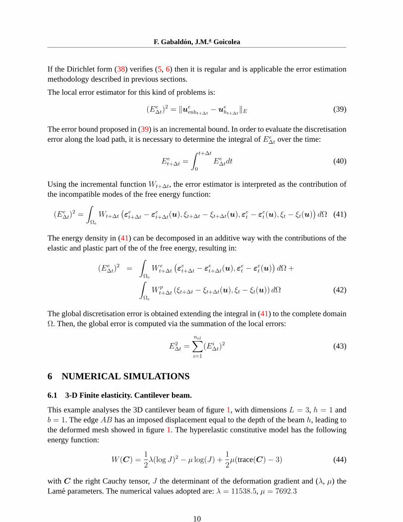
6.1 3-D Finite elasticity. Cantilever beam.

This example analyses the 3D cantilever beam of figure1, with dimensionsL = 3, h = 1 andb = 1. The edgeAB has an imposed displacement equal to the depth of the beamh, leading tothe deformed mesh showed in figure1. The hyperelastic constitutive model has the followingenergy function:

W (C) =1

2λ(log J)2 − µ log(J) +

1

2µ(trace(C)− 3) (44)

with C the right Cauchy tensor,J the determinant of the deformation gradient and (λ, µ) theLame parameters. The numerical values adopted are:λ = 11538.5, µ = 7692.3

10


L

b

h

AB

Clamped

Pinned

Time = 1.00E+00

Figure 1:3D cantilever beam. Geometry, boundary conditions and deformed mesh.

For error estimation five meshes have been considered with the following elements along length,height and thickness respectively:2× 2× 1, 4× 2× 2, 8× 4× 4, 12× 6× 6 and16× 8× 8.

Figure2 shows the curves of the energy norm obtained with enhanced elements and the globalerror estimated at the end of the computation, versus the degrees of freedom considered. Thevalues of the error estimator obtained predict an order of convergence similar to1/2: the exactone-half slope plotted in double logarithmic scale is well adjusted to the rate of convergenceobtained in the computations.

0.01

0.1

1

10

100

10 100 1000 10000

Err

or,E

nerg

y

N (DOF)

Hyperelastic cantilever

Estimated error|| ϕ ||E

Rate of convergence 1/2

Figure 2:3D cantilever beam. Evolution of global error and energy norm versus the number ofD.O.F.

Finally, figure3 shows the local error contours at the end of the process for some of the meshes.The greatest values appears near the edges with imposed displacements (AB and the clampededge).

11


6.51E-01

9.61E-01

1.27E+00

1.58E+00

1.89E+00

2.20E+00

3.40E-01

2.51E+00

L O C A L E R R O R

Current ViewMin = 3.40E-01X = 0.00E+00Y = 3.00E+00Z =-1.00E-12

Max = 2.51E+00X = 1.00E+00Y = 0.00E+00Z = 0.00E+00

Time = 1.00E+00

6.51E-01

9.61E-01

1.27E+00

1.58E+00

1.89E+00

2.20E+00

3.40E-01

2.51E+00

L O C A L E R R O R

Current ViewMin = 3.40E-01X = 0.00E+00Y = 3.00E+00Z =-1.00E-12

Max = 2.51E+00X = 1.00E+00Y = 0.00E+00Z = 0.00E+00

Time = 1.00E+00

9.76E-02

1.79E-01

2.61E-01

3.43E-01

4.24E-01

5.06E-01

1.59E-02

5.88E-01

L O C A L E R R O R

Current ViewMin = 1.59E-02X = 5.00E-01Y = 2.60E+00Z =-8.90E-01Max = 5.88E-01X = 1.00E+00Y = 0.00E+00Z = 0.00E+00

Time = 1.00E+00

9.76E-02

1.79E-01

2.61E-01

3.43E-01

4.24E-01

5.06E-01

1.59E-02

5.88E-01

L O C A L E R R O R


Time = 1.00E+00

4× 2× 2 elements 8× 4× 4 elements

4.69E-02

8.93E-02

1.32E-01

1.74E-01

2.16E-01

2.59E-01

4.62E-03

3.01E-01

L O C A L E R R O R


Time = 1.00E+00

4.69E-02

8.93E-02

1.32E-01

1.74E-01

2.16E-01

2.59E-01

4.62E-03

3.01E-01

L O C A L E R R O R


Time = 1.00E+00

3.22E-02

6.17E-02

9.11E-02

1.21E-01

1.50E-01

1.80E-01

2.75E-03

2.09E-01

L O C A L E R R O R

Current ViewMin = 2.75E-03X = 5.00E-01Y = 2.61E+00Z =-8.85E-01Max = 2.08E-01X = 5.00E-01Y = 3.00E+00Z =-1.00E-12

Time = 1.00E+00

3.22E-02

6.17E-02

9.11E-02

1.21E-01

1.50E-01

1.80E-01

2.75E-03

2.09E-01

L O C A L E R R O R

Current ViewMin = 2.75E-03X = 5.00E-01Y = 2.61E+00Z =-8.85E-01Max = 2.08E-01X = 5.00E-01Y = 3.00E+00Z =-1.00E-12

Time = 1.00E+00

8× 4× 4 elements 12× 6× 6 elements

Figure 3:3D cantilever beam. Contours of local error.

6.2 Plasticity. Undrained embankment.

The last example concerns a slope stability problem in plain strain. One half of the embankmentis considered in the analysis as shown in figure4, where the vertical face is taken to be asymmetry axis and the lateral surface subtends a45 slope. The embankment, with an increasinggravity load, rests on a rigid surface with no relative displacements over the foundation. Theanalyses were carried out with meshes of6×6, 12×12, 24×24, 36×36 and48×48 elements.

The material was assumed to exhibit undrained response resulting in no changes of volumetricstrains during deformation. The elastic properties adopted for the analysis are a Young’s modu-lusE = 2 · 108, a Poisson’s ratioν = 0.25. The material exhibits elastic-plastic behaviour withno friction angle and initial cohesionc = 2000. A constant hardening modulusH = 2 · 103 isconsidered relating the yield stress with the effective plastic strain.

The computed force-displacement curves of pointA (see figure4) for each mesh are shownin figure 5. The reference value of the gravity load is2000. In all the analyses a limit load ispredicted by the calculations.

12


12

A

24

Figure 4:Undrained embankment. Geometry and boundary conditions.

-2

-1.5

-1

-0.5

0

0.5

0 0.1 0.2 0.3 0.4 0.5 0.6 0.7

Dis

plac

emen

t(m

m)

Load factor

6× 6 elements12× 12 elements24× 24 elements36× 36 elements48× 48 elements

Figure 5:Undrained embankment. Displacement of upper left corner versus load factor.

In figure6 the global error estimator is plotted versus the number of degrees of freedom. The rateof convergence predicted is approximated equal to1/8 for the first refinement. It is remarkablethat energy increases with refinement whereas the global error decreases as the mesh is refined.

Figures7 and8 show the evolution of the elastic part and the plastic part of the accumulatedlocal error computed for the lower left element (shadowed in figure4). These values are obtainedvia the additive decomposition of the incremental error expressed in (42). Both of them decreasewith refinement of the mesh. Besides, the two components increase during the load process andtheir order of magnitude are similar. These conclusions are similar to those obtained in otherexamples ([12],[14])

Finally, figure9 shows the contours of local error computed for a load factor of0.53. The valueof local error decreases with refinement and tends to localise along a slide line.

13


0.1

1

10 100 1000 10000

Ene

rgy

N (DOF)

Error estimatedInternal energy (×102)

Rate of convergence 1/8

Figure 6:Undrained embankment. Global error versus D.O.F. (load factor= 0.53).

0

0.2

0.4

0.6

0.8

1

1.2

1.4

0 0.1 0.2 0.3 0.4 0.5 0.6

Ene

rgy

Load factor


Figure 7:Undrained embankment. Evolution of the elastic part of accumulated local error forthe lower left element.

14


0

0.2

0.4

0.6

0.8

1

1.2

1.4

1.6

0 0.1 0.2 0.3 0.4 0.5 0.6

Ene

rgy

Load factor


Figure 8:Undrained embankment. Evolution of the plastic part of accumulated local error forthe lower left element.

5.96E-04

8.48E-03

1.64E-02

2.42E-02

3.21E-02

4.00E-02

0.00E+00

2.30E-01

L O C A L E R R O R

Current ViewMin = 5.96E-04X = 2.40E+01Y = 1.20E+01

Max = 2.30E-01X = 0.00E+00Y = 0.00E+00

Time = 5.40E-01

5.96E-04

8.48E-03

1.64E-02

2.42E-02

3.21E-02

4.00E-02

0.00E+00

2.30E-01

L O C A L E R R O R


Max = 2.30E-01X = 0.00E+00Y = 0.00E+00

Time = 5.40E-01

1.02E-04

8.08E-03

1.61E-02

2.40E-02

3.20E-02

4.00E-02

0.00E+00

2.14E-01

L O C A L E R R O R


Max = 2.14E-01X = 5.00E+00Y = 0.00E+00

Time = 5.40E-01

1.02E-04

8.08E-03

1.61E-02

2.40E-02

3.20E-02

4.00E-02

0.00E+00

2.14E-01

L O C A L E R R O R


Max = 2.14E-01X = 5.00E+00Y = 0.00E+00

Time = 5.40E-01

12× 12 elements 24× 24 elements

2.97E-05

8.02E-03

1.60E-02

2.40E-02

3.20E-02

4.00E-02

0.00E+00

2.12E-01

L O C A L E R R O R


Max = 2.12E-01X = 4.67E+00Y = 0.00E+00

Time = 5.40E-01

2.97E-05

8.02E-03

1.60E-02

2.40E-02

3.20E-02

4.00E-02

0.00E+00

2.12E-01

L O C A L E R R O R


Max = 2.12E-01X = 4.67E+00Y = 0.00E+00

Time = 5.40E-01

1.24E-05

8.01E-03

1.60E-02

2.40E-02

3.20E-02

4.00E-02

0.00E+00

2.09E-01

L O C A L E R R O R


Max = 2.09E-01X = 4.50E+00Y = 0.00E+00

Time = 5.40E-01

1.24E-05

8.01E-03

1.60E-02

2.40E-02

3.20E-02

4.00E-02

0.00E+00

2.09E-01

L O C A L E R R O R


Max = 2.09E-01X = 4.50E+00Y = 0.00E+00

Time = 5.40E-01

36× 36 elements 48× 48 elements

Figure 9:Undrained embankment. Contours of local error (load factor=0.53).

15


7 CONCLUSIONS

A methodology for error estimation valid for linear and non linear problems has been described.The error estimator is based on the energy contribution of incompatible modes and in conse-quence the estimated error is zero for the patch test strain modes. It has been applied to non-linear finite elasticity and Von-Mises elastic-plastic problems with a formulation which hasvariational structure at incremental level.

The error estimator proposed establishes a measure of the discretisation error obtained withstandard elements, from the solution computed with enhanced assumed strain elements. It isformulated in a local manner and evaluated element by element without smoothing techniques.

Finally, the numerical examples analysed have shown that the results obtained with the proposedmethod for error estimation are good.

References

[1] I. Babuska and W.C. Rheinboldt. A posteriori error estimates for the finite element method.International Journal for Numerical Methods in Engineering, 12, 1597–1613, (1978).

[2] M. Ortiz and J.J. Quigley. Adaptive mesh refinement in strain localization problems.Computer Methods in Applied Mechanics and Engineering, 90, 781–804, (1991).

[3] C. Johnson and P. Hansbo. Adaptive finite element methods in computational mechanics.Computer Methods in Applied Mechanics and Engineering, 101, 143–181, (1992).

[4] F.J. Barthold, M. Schmidt, and E. Stein. Error indicators and mesh refinements for finite-element-computations of elastoplastic deformations.Computational Mechanics, 22(3),225–238, (1998).

[5] R. Radovitzky and M. Ortiz. Error estimation and adaptive meshing in strongly nonlineardynamic problems.Computer Methods in Applied Mechanics and Engineering, 172, 203–240, (1999).

[6] J.C. Simo and S.M. Rifai. A class of mixed assumed methods and the method of incompat-ible modes.International Journal for Numerical Methods in Engineering, 29, 1595–1638,(1990).

[7] J.C. Simo and F. Armero. Geometrically nonlinear enhanced strain mixed methods andthe method of incompatible modes.International Journal for Numerical Methods in En-gineering, 33, 1413–1449, (1992).

[8] J.C. Simo, F. Armero, and R.L. Taylor. Improved versions of assumed enhanced straintri-linear elements for 3d finite deformation problems.Computer Methods in AppliedMechanics and Engineering, 110, 359–386, (1993).

16


[9] F. Armero and S. Glaser. On the formulation of enhanced strain finite elements in finitedeformations.Engineering Computations, 14, 759–791, (1997).

[10] K. Washizu. Variational Methods in Elasticity & Plasticity. Pergamon Press, 3 edition,(1982).

[11] P.G. Ciarlet.The finite element method for elliptic problems. North Holland, (1978).

[12] F. Gabaldon. Metodos de elementos finitos mixtos con deformaciones supuestas en elasto-plasticidad. PhD thesis, E.T.S. Ingenieros de Caminos, Canales y Puertos. UniversidadPolitecnica de Madrid, Madrid, (1999).

[13] M. Ortiz and L. Stainier. The variational formulation of viscoplastic constitutive updates.Computer Methods in Applied Mechanics and Engineering, 171, 419–444, (1999).

[14] F. Gabaldon and J. Goicolea. Error estimation based on non-linear enhanced assumedstrain elements. In CIMNE, editor,ECCOMAS 2000, Barcelona. E. Onate, G. Bugeda andB. Suarez, (2000).

17

ERROR ESTIMATION IN FINITE ELASTICITY AND PLASTICITY...

Documents

Transcript of ERROR ESTIMATION IN FINITE ELASTICITY AND PLASTICITY...