
Error estimates for two-dimensional cross approximation
16
Journal of Approximation Theory 162 (2010) 1685–1700 www.elsevier.com/locate/jat Error estimates for two-dimensional cross approximation Jan Schneider Max Planck Institute for Mathematics in the Sciences, Inselstrasse 22, 04103 Leipzig, Germany Received 19 February 2009; accepted 24 April 2010 Available online 4 May 2010 Communicated by Paul Nevai Abstract In this paper we deal with the approximation of a given function f on [0, 1] 2 by special bilinear forms ∑ k i =1 g i ⊗ h i via the so-called cross approximation. In particular we are interested in estimating the error function f - ∑ k i =1 g i ⊗ h i of the corresponding algorithm in the maximum norm. There is a large amount of publications available that successfully deal with similar matrix algorithms in applied situations, for example in connection with H-matrices (see Boerm and Grasedyck (2003) [9] or Hackbusch (2007) [16] for many references). But as they do not give satisfactory error estimates, we concentrate on the theoretical issues of the problem in the language of functions. We connect it with related results from other areas of analysis in a historical survey and give a lot of references. Our main result is the connection of the error of our algorithm with the error of best approximation by arbitrary bilinear forms. This will be compared with the different approach in Bebendorf (2008) [6]. c 2010 Elsevier Inc. All rights reserved. Keywords: Cross approximation; Tensor products; Bilinear forms; Error estimates; Best approximation 1. Introduction and preliminaries We are basically concerned with the following question: Given a function f :[0, 1] 2 → R, how well can we approximate it by something like f ∼ k X i =1 g i ⊗ h i , (1) E-mail address: [email protected]. 0021-9045/$ - see front matter c 2010 Elsevier Inc. All rights reserved. doi:10.1016/j.jat.2010.04.012
-
Upload
jan-schneider -
Category
Documents
-
view
214 -
download
2
Transcript of Error estimates for two-dimensional cross approximation

Journal of Approximation Theory 162 (2010) 1685–1700www.elsevier.com/locate/jat
Error estimates for two-dimensional crossapproximation
Jan Schneider
Max Planck Institute for Mathematics in the Sciences, Inselstrasse 22, 04103 Leipzig, Germany
Received 19 February 2009; accepted 24 April 2010Available online 4 May 2010
Communicated by Paul Nevai
Abstract
In this paper we deal with the approximation of a given function f on [0, 1]2 by special bilinear forms∑ki=1 gi ⊗ hi via the so-called cross approximation. In particular we are interested in estimating the error
function f −∑k
i=1 gi ⊗ hi of the corresponding algorithm in the maximum norm. There is a large amountof publications available that successfully deal with similar matrix algorithms in applied situations, forexample in connection with H-matrices (see Boerm and Grasedyck (2003) [9] or Hackbusch (2007) [16]for many references). But as they do not give satisfactory error estimates, we concentrate on the theoreticalissues of the problem in the language of functions. We connect it with related results from other areas ofanalysis in a historical survey and give a lot of references. Our main result is the connection of the error ofour algorithm with the error of best approximation by arbitrary bilinear forms. This will be compared withthe different approach in Bebendorf (2008) [6].c© 2010 Elsevier Inc. All rights reserved.
Keywords: Cross approximation; Tensor products; Bilinear forms; Error estimates; Best approximation
1. Introduction and preliminaries
We are basically concerned with the following question:Given a function f : [0, 1]2 → R, how well can we approximate it by something like
f ∼k∑
i=1
gi ⊗ hi , (1)
E-mail address: [email protected].
0021-9045/$ - see front matter c© 2010 Elsevier Inc. All rights reserved.doi:10.1016/j.jat.2010.04.012
1686 J. Schneider / Journal of Approximation Theory 162 (2010) 1685–1700
i.e., by a finite sum of tensor products of one-dimensional functions (here we write (g ⊗h)(x, y) = g(x)h(y))? The right-hand side of (1) is also called a bilinear form and the firstfamous result in this direction is due to Schmidt [24], who gave a complete answer in the casef ∈ L2. A standard reference for questions in this area is [12], a nice survey can be found in [11].
In this paper we consider a very special choice of functions g, h in (1), namely the restrictionof f itself to certain lines, as will be described in what follows.
1.1. The construction
Now we describe the algorithm CA2D and fix the notation. We are given an arbitrary functionf on the unit square [0, 1]2. In the first step we choose the point (x1, y1) ∈ [0, 1]2 with f (x1,
y1) 6= 0 and define the auxiliary function
f1(x, y) =f (x1, y) f (x, y1)
f (x1, y1).
Then it is easy to see that
f1(x, y) = f (x, y) for all (x, y) ∈ C1 = {(x, y) ∈ [0, 1]2 : x = x1 ∨ y = y1}.
Hence, for the remainder we have
R1 = f − f1 = 0 on C1.
Now we want to approximate the remainder function R1 by the same idea. Therefore, we choose(x2, y2) ∈ [0, 1]2 with( f − f1)(x2, y2) 6= 0 and define
f2(x, y) =( f − f1)(x, y2)( f − f1)(x2, y)
( f − f1)(x2, y2).
Then we verify
f2 = f − f1 = R1 on C2 = {(x, y) ∈ [0, 1]2 : x = x2 ∨ y = y2}
and f2 = 0 on C1, hence
f1 + f2 = f on G2 = C1 ∪ C2 and so R2 = f − f1 − f2 = 0 on G2.
We go on with this scheme and define for j ∈ N the iterative expression
f j (x, y) =
(f −
j−1∑i=1
fi
)(x j , y)
(f −
j−1∑i=1
fi
)(x, y j )(
f −j−1∑i=1
fi
)(x j , y j )
,
where the pivot points (x j , y j ) are always chosen such that(f −
j−1∑i=1
fi
)(x j , y j ) 6= 0.
J. Schneider / Journal of Approximation Theory 162 (2010) 1685–1700 1687
For a detailed discussion about how to choose those points we refer to the next subsection. Thefunction given by
Fk(x, y) =k∑
j=1
f j (x, y)
is the resulting kth interpolation function of f via this algorithm, the two-dimensional crossapproximation (CA2D). We observe that Fk has the property of the right-hand side of (1) as asum of products of one-dimensional functions. By repeating the same arguments as before, onecan prove
Fk(x, y) = f (x, y) for all (x, y) ∈ Gk =
k⋃j=1
C j ,
where C j = {(x, y) ∈ [0, 1]2 : x = x j ∨ y = y j }, hence,
Rk(x, y) := f (x, y)− Fk(x, y) = 0 for all (x, y) ∈ Gk (2)
for k ∈ N. So one can think of Rk as a function that lives inside of small rectangles and vanisheson their edges. By the above construction we have
Rk(x, y) = Rk−1(x, y)−Rk−1(x, yk)Rk−1(xk, y)
Rk−1(xk, yk), (3)
which also shows, how to recursively implement CA2D.
1.2. Questions
Our main goal is to estimate the maximum norm of the CA2D error function Rk by the errorof best approximation by bilinear forms. This will be done in Section 4 for functions eitherbelonging to the space C([0, 1]2) of continuous functions or to the space L∞([0, 1]2) of boundedfunctions. There are some questions related to this, for example: What are the influences ofsmoothness and structural properties of f ? We discuss those issues in Section 2.
The point we want to treat now is the choice of the pivot elements (x j , y j ). At the first glanceit seems reasonable to choose the remaining maximum of the error in [0, 1]2 (full pivoting), i.e.(
f −j−1∑i=1
fi
)(x j , y j ) = max
(x,y)∈[0,1]2
(f −
j−1∑i=1
fi
)(x, y) 6= 0,
to minimize the error after the next step. But as soon as it comes to the implementation,one of course intends to avoid full pivoting. Therefore, another alternative was considered(partial pivoting), see [5], where the x-coordinates of the crosses are chosen randomly such thatRk(xk+1, y) does not vanish for all y ∈ [0, 1] and the y-coordinates as the maxima on the line.When we implemented CA2D for testing we used an even more restrictive algorithm (specialpivoting), where the xk are determined by the following procedure: x1 = 1/2, x2 = 1/4, x3 =
3/4 and going on from left to right by always dividing the remaining intervals in the middle.The y-coordinates are again the maxima on the line. (One has to be careful here with symmetricfunctions!). We will see in Sections 3 and 4 that there is also another pivot strategy of interestcalled maximal-volume concept, see [14], we will discuss it at the end of 3.1. However, someresults of the following section are even independent of such a strategy.
1688 J. Schneider / Journal of Approximation Theory 162 (2010) 1685–1700
2. Basic results
We start with an observation already mentioned as formula (2) in 1.1. Using the notation in-troduced there we will formulate it as Proposition and refer to it later on as interpolation property.
Proposition 2.1. For any function f : [0, 1]2 → R, we have
Rk(x, y) = 0 for all (x, y) ∈ Gk .
The next result takes an a priori knowledge about structural properties of the underlying functioninto account. We say that a function f has separation rank k, if one can represent it as
f (x, y) =k∑
i=1
gi (x)hi (y)
and there is no such representation with reduced summing order. We call the following the rankproperty.
Proposition 2.2. Let f have separation rank k. Then CA2D reproduces f after k steps exactly,that means
Rk = f − Fk = 0 on [0, 1]2.
A matrix version of this result was first proved in [5] (Lemma 7).
Proof. We will prove that Rk′ = f − Fk′ has separation rank k − k′ for k′ ∈ {0, 1, . . . , k} byinduction. For k′ = 0 there is nothing to prove, so let for k′ < k the function Rk′ have separationrank k − k′. We define
V = span{Rk′(·, y) : y ∈ [0, 1]}
and
V ′ = span{Rk′+1(·, y) : y ∈ [0, 1]}.
We know that dim V = k − k′ and want to show dim V ′ = k − k′ − 1. For each y ∈ [0, 1] wewrite with the notation of Section 1.1 (formula (3))
Rk′+1(x, y) = Rk′(x, y)−Rk′(x, yk′+1)Rk′(xk′+1, y)
Rk′(xk′+1, yk′+1)
and see, that both terms on the right-hand side belong to V , hence V ′ ⊂ V . Furthermore,we know Rk′(·, yk′+1) ∈ V but because Rk′(xk′+1, yk′+1) 6= 0 and Rk′+1(xk′+1, y) = 0 forall y ∈ [0, 1], there is no representation of Rk′(·, yk′+1) as a linear combination of functionsRk′+1(·, y), hence Rk′(·, yk′+1) 6∈ V ′. It follows dim V ′ < dim V and because those dimensionscan differ at most by one, we get dim V ′ = dim V − 1 = k − k′ − 1. Now we know that for ally ∈ [0, 1] we have a representation
Rk′+1(x, y) =k−k′−1∑
i=1
αi,yϕi (x)
with coefficients αi,y and functions ϕi (x). If we now identify ψi (y) = αi,y , we conclude thatRk′+1 has separation rank k − (k′ + 1). �
J. Schneider / Journal of Approximation Theory 162 (2010) 1685–1700 1689
This result tells us that the algorithm is exact, if f has already a tensor product structure as in(1), even if f is not smooth at all. Besides that one would expect that CA2D converges faster iff shares some nice smoothness properties. To get an explicit estimate for a more general classof functions determined by the smoothness, we follow the basic idea appearing for polynomialinterpolation on an interval. For that we define
ωk(x) =k∏
i=1
(x − xi )
and denote by f (k)x the kth partial derivative of f with respect to x .
Proposition 2.3. Let f ∈ Ck([0, 1]2). Then the error of CA2D with partial pivoting can beestimated by
|Rk(x, y)| ≤|ωk(x)|
k!2k sup
x∈[0,1]| f (k)x (x, y)|. (4)
Proof. We fix (x, y) ∈ [0, 1]2 and define
F(x) = Rk(x, y)− Kωk(x).
Now we determine K such that F(x) = 0. Then F has at least n + 1 zeros in [0, 1], henceF (k)(ξ) = 0 for ξ ∈ [0, 1]. We find
K =R(k)k (ξ, y)
k!,
where the derivative is with respect to the first variable, and because of |R(k)k (x, y)| ≤ 2k| f (k)x
(x, y)| we can estimate
|Rk(x, y)| = |Kωk(x)| ≤|ωk(x)|
k!2k| f (k)x (ξ, y)|,
which finishes the proof. �
Let us discuss this result. First one observes, that it is basically one-dimensional, where thebehavior in the other direction is not taken into account. So one can do the same argumentationwith respect to y and the corresponding assertion would also be true. That means the error Rk isbounded by the expression (4) with respect to x or y, therefore,
|Rk(x, y)| ≤2k
k!min
(|ωx
k (x)| supx∈[0,1]
| f (k)x (x, y)|, |ωyk (y)| sup
y∈[0,1]| f (k)y (x, y)|
).
But that of course does not change the quality of the estimate. We tested the algorithm withour special pivoting for the function f (x, y) = exp(−xy), where | f (k)x (x, y)| ≤ 1. After 15steps the error of CA2D was 5.2479 · 10−15, where estimate (4) gives 2.8422 · 10−14. This seemsreasonable, but the situation changes dramatically if the partial derivatives of f are not uniformlybounded. We tested also f (x, y) = sin(10xy), where the corresponding factor in (4) grows like10k , here the algorithm gave after 15 steps an error of 2.8084 · 10−11 but our estimate gives28.422. That means, derivatives of f itself cannot be a suitable factor in the error estimate, butof course smoothness should influence it somehow. So observing that Rk does not change after
1690 J. Schneider / Journal of Approximation Theory 162 (2010) 1685–1700
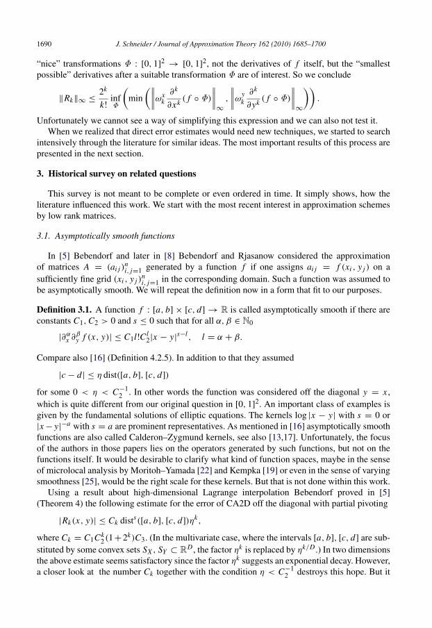
“nice” transformations Φ : [0, 1]2 → [0, 1]2, not the derivatives of f itself, but the “smallestpossible” derivatives after a suitable transformation Φ are of interest. So we conclude
‖Rk‖∞ ≤2k
k!infΦ
(min
(∥∥∥∥ωxk∂k
∂xk ( f ◦ Φ)∥∥∥∥∞
,
∥∥∥∥ωyk∂k
∂yk ( f ◦ Φ)∥∥∥∥∞
)).
Unfortunately we cannot see a way of simplifying this expression and we can also not test it.When we realized that direct error estimates would need new techniques, we started to search
intensively through the literature for similar ideas. The most important results of this process arepresented in the next section.
3. Historical survey on related questions
This survey is not meant to be complete or even ordered in time. It simply shows, how theliterature influenced this work. We start with the most recent interest in approximation schemesby low rank matrices.
3.1. Asymptotically smooth functions
In [5] Bebendorf and later in [8] Bebendorf and Rjasanow considered the approximationof matrices A = (ai j )
ni, j=1 generated by a function f if one assigns ai j = f (xi , y j ) on a
sufficiently fine grid (xi , y j )ni, j=1 in the corresponding domain. Such a function was assumed to
be asymptotically smooth. We will repeat the definition now in a form that fit to our purposes.
Definition 3.1. A function f : [a, b] × [c, d] → R is called asymptotically smooth if there areconstants C1,C2 > 0 and s ≤ 0 such that for all α, β ∈ N0
|∂αx ∂βy f (x, y)| ≤ C1l!C l
2|x − y|s−l , l = α + β.
Compare also [16] (Definition 4.2.5). In addition to that they assumed
|c − d| ≤ η dist([a, b], [c, d])
for some 0 < η < C−12 . In other words the function was considered off the diagonal y = x ,
which is quite different from our original question in [0, 1]2. An important class of examples isgiven by the fundamental solutions of elliptic equations. The kernels log |x − y| with s = 0 or|x− y|−a with s = a are prominent representatives. As mentioned in [16] asymptotically smoothfunctions are also called Calderon–Zygmund kernels, see also [13,17]. Unfortunately, the focusof the authors in those papers lies on the operators generated by such functions, but not on thefunctions itself. It would be desirable to clarify what kind of function spaces, maybe in the senseof microlocal analysis by Moritoh–Yamada [22] and Kempka [19] or even in the sense of varyingsmoothness [25], would be the right scale for these kernels. But that is not done within this work.
Using a result about high-dimensional Lagrange interpolation Bebendorf proved in [5](Theorem 4) the following estimate for the error of CA2D off the diagonal with partial pivoting
|Rk(x, y)| ≤ Ck dists([a, b], [c, d])ηk,
where Ck = C1Ck2 (1+2k)C3. (In the multivariate case, where the intervals [a, b], [c, d] are sub-
stituted by some convex sets SX , SY ⊂ RD , the factor ηk is replaced by ηk/D .) In two dimensionsthe above estimate seems satisfactory since the factor ηk suggests an exponential decay. However,a closer look at the number Ck together with the condition η < C−1
2 destroys this hope. But it

J. Schneider / Journal of Approximation Theory 162 (2010) 1685–1700 1691
was still a big improvement in terms of explicit error estimates for CA2D in comparison with ear-lier results concerning for example the so-called Pseudoskeleton Approximations by Goreinov,Tyrtyshnikov and Zamarashkin, see [15]. Also in [5] Bebendorf mentions the maximum-volumeconcept to control the error of CA2D. This concept proposes to choose the pivots (xi , yi ) suchthat the absolute value of the determinant det
(f (xi , y j )
)ki, j=1 is maximal. That is of course prac-
tically not acceptable but because of the nice formula
k∏i=0
Ri (xi+1, yi+1) = det(
f (xi , y j ))k+1
i, j=1 , (5)
for all k ∈ N (which you can also find in [5], Lemma 2), we can see, that partial pivoting isthe best strategy with respect to maximal determinants if we want to keep all previous pivotsfixed. Much work concerning asymptotically smooth functions and the maximal-volume conceptin connection with the numerical application was done for example by Tyrtyshnikov, see [29],where also some more references are given.
We recently learned that Bebendorf connected the CA2D error with some kind of bestapproximation in [6], where a matrix version of it can already be found in [7]. Since this isalso one aim of our paper we will compare his technique with our approach in Section 4.2. In thenext subsections we examine older examples in the literature that are already very close to ourpurposes.
3.2. Totally positive functions
Already more than thirty years ago, Micchelli and Pinkus wrote a very interesting paper [21]concerning the approximation problem (1) in mixed p, q-norms. The main assumption on theirfunctions was total positivity. Here we repeat the definition.
Definition 3.2. A real valued kernel K (x, y) continuous on [0, 1]2 is called totally positive if allits Fredholm minors
K
(s1, . . . , sm
t1, . . . , tm
)= det
(K (si , t j )
)mi, j=1 =
∣∣∣∣∣∣∣K (s1, t1) · · · K (s1, tm)
......
K (sm, t1) · · · K (sm, tm)
∣∣∣∣∣∣∣are nonnegative for 0 ≤ s1 < · · · < sm ≤ 1, 0 ≤ t1 < · · · < tm ≤ 1 and all m ≥ 1.
For further details about total positivity see [18], where also many examples are given. Micchelliand Pinkus were concerned with finding the best approximation by bilinear forms, i.e.
Enp,q(K ) = inf
∣∣∣∣∣K − n∑
i=1
ui ⊗ vi
∣∣∣∣∣p,q
,where the infimum is taken over all u1, . . . , un ∈ L p
[0, 1] and v1, . . . , vn ∈ Lq[0, 1] and
|K |p,q =
∫ 1
0
(∫ 1
0|K (x, y)qdy
)p/q
dx
1/p
, (6)
for 1 ≤ p, q ≤ ∞. That is exactly our problem (1) in these mixed norms restricted to those spe-cial functions. Before we state their results we need some preparation. By the notation in [21] let
1692 J. Schneider / Journal of Approximation Theory 162 (2010) 1685–1700
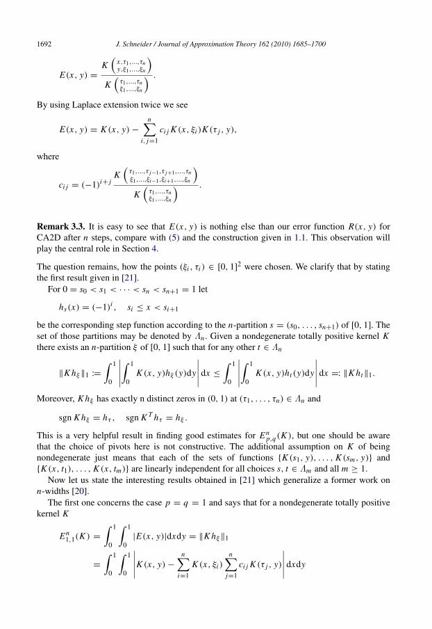
E(x, y) =K(
x,τ1,...,τny,ξ1,...,ξn
)K(τ1,...,τnξ1,...,ξn
) .By using Laplace extension twice we see
E(x, y) = K (x, y)−n∑
i, j=1
ci j K (x, ξi )K (τ j , y),
where
ci j = (−1)i+ jK(τ1,...,τ j−1,τ j+1,...,τnξ1,...,ξi−1,ξi+1,...,ξn
)K(τ1,...,τnξ1,...,ξn
) .
Remark 3.3. It is easy to see that E(x, y) is nothing else than our error function R(x, y) forCA2D after n steps, compare with (5) and the construction given in 1.1. This observation willplay the central role in Section 4.
The question remains, how the points (ξi , τi ) ∈ [0, 1]2 were chosen. We clarify that by statingthe first result given in [21].
For 0 = s0 < s1 < · · · < sn < sn+1 = 1 let
hs(x) = (−1)i , si ≤ x < si+1
be the corresponding step function according to the n-partition s = (s0, . . . , sn+1) of [0, 1]. Theset of those partitions may be denoted by Λn . Given a nondegenerate totally positive kernel Kthere exists an n-partition ξ of [0, 1] such that for any other t ∈ Λn
‖K hξ‖1 :=∫ 1
0
∣∣∣∣∣∫ 1
0K (x, y)hξ (y)dy
∣∣∣∣∣ dx ≤∫ 1
0
∣∣∣∣∣∫ 1
0K (x, y)ht (y)dy
∣∣∣∣∣ dx =: ‖K ht‖1.
Moreover, K hξ has exactly n distinct zeros in (0, 1) at (τ1, . . . , τn) ∈ Λn and
sgn K hξ = hτ , sgn K T hτ = hξ .
This is a very helpful result in finding good estimates for Enp,q(K ), but one should be aware
that the choice of pivots here is not constructive. The additional assumption on K of beingnondegenerate just means that each of the sets of functions {K (s1, y), . . . , K (sm, y)} and{K (x, t1), . . . , K (x, tm)} are linearly independent for all choices s, t ∈ Λm and all m ≥ 1.
Now let us state the interesting results obtained in [21] which generalize a former work onn-widths [20].
The first one concerns the case p = q = 1 and says that for a nondegenerate totally positivekernel K
En1,1(K ) =
∫ 1
0
∫ 1
0|E(x, y)|dxdy = ‖K hξ‖1
=
∫ 1
0
∫ 1
0
∣∣∣∣∣K (x, y)−n∑
i=1
K (x, ξi )
n∑j=1
ci j K (τ j , y)
∣∣∣∣∣ dxdy
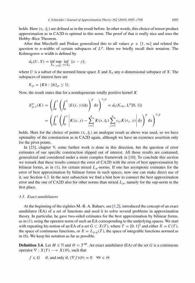
J. Schneider / Journal of Approximation Theory 162 (2010) 1685–1700 1693
holds. Here (τi , ξi ) are defined as in the result before. In other words, this choice of tensor productapproximation as in CA2D is optimal in this norm. The proof of that is really nice and uses theHobby–Rice Theorem.
After that Micchelli and Pinkus generalized this to all values p ∈ [1,∞] and related thequestion to n-widths of certain subspaces of L p. Here we briefly recall their notation. TheKolmogorov n-width is defined by
dn(U, X) = infXn
supx∈U
infy∈Xn‖x − y‖,
where U is a subset of the normed linear space X and Xn any n-dimensional subspace of X . Thesubspaces of interest here are
K p = {K h : ‖h‖p ≤ 1}.
Now, the result states that for a nondegenerate totally positive kernel K
Enp,1(K ) =
(∫ 1
0
(∫ 1
0|E(x, y)|dy
)p
dx
)1/p
= dn(K∞, L p[0, 1])
=
(∫ 1
0
(∫ 1
0
∣∣∣∣∣K (x, y)−n∑
i=1
K (x, ξi )
n∑j=1
ci j K (τ j , y)
∣∣∣∣∣ dy
)p
dx
)1/p
holds. Here for the choice of points (τi , ξi ) an analogue result as above was used, so we haveoptimality of the construction as in CA2D again, although we have an existence assertion onlyfor the pivot points.
In [23], chapter V, some further work is done in this direction, but the question of errorestimates of our specific construction slipped out of interest. All those results are contained,generalized and considered under a more complex framework in [10]. To conclude this sectionwe remark that these results connect the error of CA2D with the error of best approximation bybilinear forms, as in (1), for certain mixed L p-norms. If one has asymptotic estimates for theerror of best approximation by bilinear forms in such spaces, now one can make direct use ofit, see Section 4.3. In the next subsection we find a hint how to connect the best approximationerror and the one of CA2D also for other norms than mixed L p, namely for the sup-norm in thefirst place.
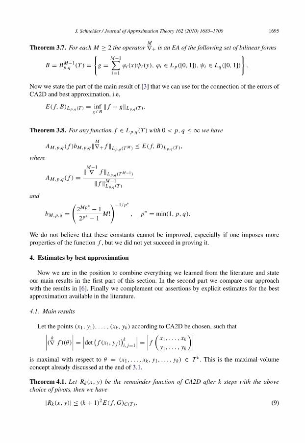
3.3. Exact annihilators
At the beginning of the eighties M.-B. A. Babaev, see [1,2], introduced the concept of an exactannihilator (EA) of a set of functions and used it to solve several problems in approximationtheory. In particular, he gave two-sided estimates for the best approximation by bilinear forms,as in (1), using the operator norm of such an EA corresponding to the underlying spaces. We startwith repeating his notion of an EA of a set G ⊂ X (T ), where T = [0, 1]2 and either X = C(T ),the space of continuous functions, or X = L p,q(T ), the space of integrable functions normed asin (6). We keep his notation as far as possible.
Definition 3.4. Let M ∈ N and Θ = T M . An exact annihilator (EA) of the set G is a continuousoperator ∇ : X (T ) −→ X (Θ), such that
f ∈ G if, and only if, (∇ f )(θ) = 0 ∀θ ∈ Θ .

1694 J. Schneider / Journal of Approximation Theory 162 (2010) 1685–1700
Because our main goal in this paper is to get information about the error of CA2D in themaximum norm we concentrate now on the cases X = C and X = L∞ separately.
3.3.1. The case C([0, 1]2)All what follows in this part can be found in [1]. For θ = (x1, . . . , xM , y1, . . . , yM ) ∈ Θ we
define the operatorM∇∗ by
(M∇∗ f )(θ) =
(
M∇ f )(θ)
‖M−1∇ f ‖C(T M−1)
, (M∇ f )(θ) 6= 0,
0, (M∇ f )(θ) = 0.
where (M∇ f )(θ) = det
(f (xi , y j )
)Mi, j=1.
Theorem 3.5. For each M ≥ 2 the operatorM∇∗ is an EA of the following set of bilinear forms
G = G M−1C (T ) =
{g =
M−1∑i=1
ϕi (x)ψi (y), ϕi , ψi ∈ C([0, 1])
}. (7)
Here we already see that some close connection between this operator and the error of CA2Dseems possible. If we interpret θ = (x1, . . . , xM , y1, . . . , yM ) ∈ Θ as the set of pivot coordinatesand keep Remark 3.3 in mind, obviously the Theorem above reminds us of the rank property ofCA2D in Proposition 2.2. Now we state the main result of [1] from which we can establish theconnection of the errors of CA2D and best approximation, i.e,
E( f,G)C(T ) = infg∈G‖ f − g‖C(T ). (8)
Theorem 3.6. For any function f ∈ C(T ) we have
1/M2‖M∇∗ f ‖C(T M ) ≤ E( f,G)C(T ) ≤ ‖
M∇∗ f ‖C(T M ).
This result is one of the keys to our main results in Section 4. Because CA2D does not requirecontinuity we assume only boundedness in the next part.
3.3.2. The case L∞([0, 1]2)In [3] Babaev used the concept of an exact annihilator to attack the problem of estimating the
best approximation by bilinear forms in mixed L p spaces including L∞. We state his results inthis part in full generality even though we are most interested in the L∞ versions, which we willuse afterwards to find a concrete error estimate for CA2D.
For θ = (x1, . . . , xM , y1, . . . , yM ) ∈ Θ we define the operatorM∇+ by
(M∇+ f )(θ) =
(
M∇ f )(θ)
‖M−1∇ f ‖L p,q (T M−1)
, (M∇ f )(θ) 6= 0,
0, (M∇ f )(θ) = 0
where (M∇ f )(θ) = det
(f (xi , y j )
)Mi, j=1 has the same meaning as in the previous case.
J. Schneider / Journal of Approximation Theory 162 (2010) 1685–1700 1695
Theorem 3.7. For each M ≥ 2 the operatorM∇+ is an EA of the following set of bilinear forms
B = B M−1p,q (T ) =
{g =
M−1∑i=1
ϕi (x)ψi (y), ϕi ∈ L p([0, 1]), ψi ∈ Lq([0, 1])
}.
Now we state the part of the main result of [3] that we can use for the connection of the errors ofCA2D and best approximation, i.e,
E( f, B)L p,q (T ) = infg∈B‖ f − g‖L p,q (T ).
Theorem 3.8. For any function f ∈ L p,q(T ) with 0 < p, q ≤ ∞ we have
AM,p,q( f )bM,p,q‖M∇+ f ‖L p,q (T M ) ≤ E( f, B)L p,q (T ),
where
AM,p,q( f ) =‖
M−1∇ f ‖L p,q (T M−1)
‖ f ‖M−1L p,q (T )
and
bM,p,q =
(2Mp∗
− 12p∗ − 1
M !
)−1/p∗
, p∗ = min(1, p, q).
We do not believe that these constants cannot be improved, especially if one imposes moreproperties of the function f , but we did not yet succeed in proving it.
4. Estimates by best approximation
Now we are in the position to combine everything we learned from the literature and stateour main results in the first part of this section. In the second part we compare our approachwith the results in [6]. Finally we complement our assertions by explicit estimates for the bestapproximation available in the literature.
4.1. Main results
Let the points (x1, y1), . . . , (xk, yk) according to CA2D be chosen, such that∣∣∣∣( k∇ f )(θ)
∣∣∣∣ = ∣∣∣det(
f (xi , y j ))k
i, j=1
∣∣∣ = ∣∣∣∣ f
(x1, . . . , xk
y1, . . . , yk
)∣∣∣∣is maximal with respect to θ = (x1, . . . , xk, y1, . . . , yk) ∈ T k . This is the maximal-volumeconcept already discussed at the end of 3.1.
Theorem 4.1. Let Rk(x, y) be the remainder function of CA2D after k steps with the abovechoice of pivots, then we have
|Rk(x, y)| ≤ (k + 1)2 E( f,G)C(T ). (9)
1696 J. Schneider / Journal of Approximation Theory 162 (2010) 1685–1700
Proof. By Remark 3.3 we have the following identity
|Rk(x, y)| =
∣∣∣∣∣∣f(
x,x1,...,xky,y1,...,yk
)f(
x1,...,xky1,...,yk
)∣∣∣∣∣∣ .
Because of the special choice of pivots we can for θ = (x, x1, . . . , xm, y, y1, . . . , ym) write
|Rk(x, y)| =
∣∣∣∣∣∣ (k+1∇ f )(θ)
‖k∇ f ‖C(T k )
∣∣∣∣∣∣ .Using Definition 3.4 and Theorem 3.6 we can conclude
|Rk(x, y)| =
∣∣∣∣(k+1∇ ∗ f )(θ)
∣∣∣∣ ≤ ‖k+1∇ ∗ f ‖C(T k+1) ≤ (k + 1)2 E( f,G)C(T ). �
The proof of Theorem 4.1 allows an immediate generalization in terms of the pivot strategy.Let now the points (x1, y1), . . . , (xk, yk) be chosen, such that
‖k∇ f ‖C(T k ) ≤ τ
∣∣∣∣ f
(x1, . . . , xm
y1, . . . , ym
)∣∣∣∣for a real number τ ≥ 1.
Corollary 4.2. With the above notation we have
|Rk(x, y)| ≤ τ(k + 1)2 E( f,G)C(T ).
Finally, we established an estimate of the error of CA2D for continuous functions from aboveby the error of best approximation by arbitrary bilinear forms. If there would be an explicitestimate of E( f,G)C(T ) for special functions f (say smooth) available, one could immediatelyplug it in here to obtain a concrete estimate for CA2D. For the next case, we will follow thisidea in Section 4.3. Now we state the analogue of Theorem 4.1 for the L∞-norm. Let the points(x1, y1), . . . , (xk, yk) according to CA2D be chosen, such that∣∣∣∣( k
∇ f )(θ)
∣∣∣∣ = ‖ k∇ f ‖L∞(T k ).
Then we can state:
Theorem 4.3. Let Rk(x, y) be the remainder function of CA2D after k steps with the abovechoice of pivots, then we have
|Rk(x, y)| ≤ (2k+1− 1)(k + 1)!
‖ f ‖kL∞(T )
‖k∇ f ‖L∞(T k )
E( f, B)L∞(T ).
The idea of the proof is exactly the same as for Theorem 4.1, one can follow it line by line. Alsoin analogy to the case of C([0, 1]2) we can formulate an easy modification. Let now the points(x1, y1), . . . , (xk, yk) be chosen, such that
‖k∇ f ‖L∞(T k ) ≤ τ
∣∣∣∣( k∇ f )(θ)
∣∣∣∣
J. Schneider / Journal of Approximation Theory 162 (2010) 1685–1700 1697
for a real number τ ≥ 1.
Corollary 4.4. With the above notation we have
|Rk(x, y)| ≤ τ(2k+1− 1)(k + 1)!
‖ f ‖kL∞(T )
‖k∇ f ‖L∞(T k )
E( f, B)L∞(T ).
Because of the bad looking constants this result lost some beauty. Nevertheless, we use it in thelast part to show how explicit error estimates for CA2D can be produced.
4.2. A comparison
Now we briefly compare the estimates achieved in the previous section with similar results byBebendorf in [6] obtained by a different method. His aim there is to estimate the CA2D error Rkby the best approximation in an arbitrary system Ξ of functions ξ1(y), . . . , ξk(y) in the sense
|Rk(x, y)| ≤ c infΞ
supx∈[0,1]
infp∈span Ξ
‖ f (x, ·)− p‖∞,[0,1], (10)
where originally the domains are more general than [0, 1]2. Using Lagrange interpolation tech-niques he found the following estimate for CA2D with maximal-volume concept in any system Ξ
|Rk(x, y)| ≤ (k + 1)(1+ ‖IΞk ‖) sup
x∈[0,1]inf
p∈span Ξ‖ f (x, ·)− p‖∞,[0,1], (11)
where
‖IΞk ‖ = max
f ∈C([0,1])
{‖IΞ
k f ‖∞,[0,1]/‖ f ‖∞,[0,1]}
is called the Lebesgue constant of the interpolation operator
IΞk f =
k∑l=1
f (yl)LΞl
with LΞl being the Lagrange functions for ξl(y) and yl ∈ [0, 1], l = 1, . . . , k. It is not clear how
to compare (11) with our corresponding estimate (9) directly, because of the unknown factor‖IΞ
k ‖. But in some sense this result fits quite well into our picture since if we take a closer lookto the best approximation defined in (8) over the set (7) with M = k + 1, then we observe
E( f,G)C(T ) = infψ1,...,ψk∈C([0,1])
infϕ1,...,ϕk∈C([0,1])
supx∈[0,1]
‖ f (x, ·)−k∑
i=1
ϕi (x)ψi (y)‖∞,[0,1]
≥ infΞ
supx∈[0,1]
infp∈span Ξ
‖ f (x, ·)− p‖∞,[0,1],
because the functions ξ1(y), . . . , ξk(y) are completely arbitrary.Also in [6] Bebendorf gave an elegant estimate by the best approximation in (10) for the CA2D
error with partial pivoting in the same fashion. We were not able to achieve a correspondingestimate by our method.

1698 J. Schneider / Journal of Approximation Theory 162 (2010) 1685–1700
4.3. Explicit estimates
In this section we complement the results obtained in Section 4.1 by two-sided error estimatesfor the best approximation by bilinear forms available in the literature. We concentrate here onthe papers published by Babaev (see [4]) and Temlyakov (see for example [26–28]). They wereconcerned with the following question: What is the exact asymptotic behavior of the quantities
τM ( f )p1,p2 = infui ,vi ;i=1,...,M
∥∥∥∥∥ f (x, y)−M∑
i=1
ui (x)vi (y)
∥∥∥∥∥p1,p2
and
τM (F)p1,p2 = supf ∈F
τM ( f )p1,p2
for various choices of function classes F? Here we keep the notation for best approximation usedby these authors.
Babaev concentrated on the unit ball of the classical Sobolev class W rq (T ), where Temlyakov
treated periodic functions f defined on the 2d-dimensional torus π2d belonging to a Sobolevclass with bounded mixed derivatives. We will formulate some of their results in a commonnotation.
A typical result in Temlyakov’s papers, obtained in [26] for p1 = p2 = p, looks like
τM (Wrq,α)p ∼
M−2r+1/q−1/p, 1 ≤ q ≤ p ≤ 2, r > 1/q − 1/p,M−2r , 2 ≤ q, p ≤ ∞, r > 1/2,M−2r+1/q−1/2, 1 ≤ q < 2 < p ≤ ∞, r > 1/q.
for r = (r1, r2) = r .For our purposes the results of Babaev [4] fit better to our needs. He found
τM (Wrq )p ∼ M−r
for all 2 ≤ q ≤ p ≤ ∞ and r > 2/q − 1/p.Now we combine this result with Corollary 4.4 to establish a quantitative error estimate of
CA2D in the L∞-norm.
Theorem 4.5. With the assumptions of Corollary 4.4 we have for all f belonging to the unit ballof W r
∞(T )
|Rk(x, y)| ≤ cτ(2k+1− 1)(k + 1)!
(k + 1)−r
‖k∇ f ‖L∞(T k )
.
This estimate surely suffers again from the k-dependence of the constants. But one could arguethe following way : If we assume f to be very smooth, we can reach a very large r in the estimate.Since we know by experiments that CA2D converges very fast for nice functions, we only needto consider small values of k and the terms blowing up with k would not destroy the nice flavor ofthe estimate. But of course it is desirable to improve the constants, which we postpone to furtherwork.
J. Schneider / Journal of Approximation Theory 162 (2010) 1685–1700 1699
Acknowledgments
The author thanks Prof. W. Hackbusch (Max Planck Institute for Mathematics in the Sciences,Leipzig, Germany), Prof. M. Bebendorf (University of Bonn, Germany) as well as Prof. E. Novakand Prof. W. Sickel (both Friedrich Schiller University, Jena, Germany) for inspiring discussions.
References
[1] M.-B.A. Babaev, Best approximation by bilinear forms, Mat. Zametki 46 (2) (1989) 21–33.[2] M.-B.A. Babaev, Exact annihilators and their applications in approximation theory, Trans. Acad. Sci. Azerb. Ser.
Phys. Tech. Math. Sci. 20 (1) (2000); Math. Mech. 233 17–24.[3] M.-B.A. Babayev, On estimation of the best approximation by bilinear forms in space with mixed norm, Trans.
Acad. Sci. Azerb. Ser. Phys. Tech. Math. Sci. 24 (4) (2004); Math. Mech., 23–32.[4] M.-B.A. Babaev, Approximation of the Sobolev classes W r
q of functions of several variables by bilinear forms inL p for 2 ≤ q ≤ p ≤ ∞, Mat. Zametki 62 (1) (1997) 18–34. (translation in Math. Notes 62 (1997) (1–2) 15–29(1998)) (in Russian).
[5] M. Bebendorf, Approximation of boundary element matrices, Numer. Math. 86 (2000) 565–589.[6] M. Bebendorf, Hierarchical Matrices. Lecture Notes in Computational Science and Engineering, vol. 63, Springer-
Verlag, Berlin, 2008.[7] M. Bebendorf, R. Grzhibovskis, Accelerating Galerkin BEM for linear elasticity using adaptive cross
approximation, Math. Methods Appl. Sci. 29 (2006) 1721–1747.[8] M. Bebendorf, S. Rjasanow, Adaptive low-rank approximation of collocation matrices, Computing 70 (2003) 1–24.[9] S. Boerm, L. Grasedyck, W. Hackbusch, Hierarchical matrices, in: Max Planck Institute for Mathematics in the
Sciences, in: Lecture Note, vol. 21, 2003.[10] A.L. Brown, Finite rank approximations to integral operators which satisfy certain total positivity conditions, J.
Approx. Theory 34 (1982) 42–90.[11] E.W. Cheney, The Best Approximation of Multivariate Functions by Combinations of Univariate Ones,
in: Approximation theory, vol. IV, Academic Press, New York, 1983, pp. 1–26 (College Station, Tex., 1983).[12] E.W. Cheney, W.A. Light, Approximation Theory in Tensor Product Spaces, in: Lecture Notes in Mathematics, vol.
1169, Springer-Verlag, 1985.[13] R. Coifman, Y. Meyer, Wavelets and Operators II, Calderon–Zygmund and multilinear operators, in: Cambridge
Studies in Advanced Mathematics, vol. 48, Cambridge University Press, Cambridge, 1997.[14] S.A. Goreinov, E.E. Tyrtyshnikov, The maximal-volume concept in approximation by low-rank matrices, Contemp.
Math. 280 (2001).[15] S.A. Goreinov, E.E. Tyrtyshnikov, N.L. Zamarashkin, A theory of pseudoskeleton approximations, Linear Algebra
Appl. 261 (1997) 1–21.[16] W. Hackbusch, Hierarchische Matrizen — Algorithmen und Analysis, in: Lecture Notes of Max Planck Institute
for Mathematics in the Sciences, Leipzig, 2007.[17] S. Jaffard, Y. Meyer, Wavelet methods for pointwise regularity and local oscillations of functions, Mem. Amer.
Math. Soc. 123 (1996) 587.[18] S. Karlin, Total Positivity, vol. 1, Stanford Univ. Press, Stanford, Calif, 1968.[19] H. Kempka, Atomic, molecular and wavelet decomposition of generalized 2-microlocal Besov spaces, J. Funct.
Spaces Appl. (2010) (in press).[20] C.A. Micchelli, A. Pinkus, On n-widths in L∞, Trans. Amer. Math. Soc. 234 (1977) 139–174.[21] C.A. Micchelli, A. Pinkus, Some problems in the approximation of functions of two variables and n-widths of
integral operators, J. Approx. Theory 24 (1978) 51–77.[22] S. Moritoh, T. Yamada, Two-microlocal Besov spaces and wavelets, Rev. Mat. Iberoam. 20 (2004) 277–283.[23] A. Pinkus, N -Widths in Approximation Theory. Ergebnisse der Mathematik und ihrer Grenzgebiete, 3.Folge, Band
7, Springer, 1985.[24] E. Schmidt, Zur Theorie der linearen und nicht linearen Integralgleichungen, I., Math. Ann. 63 (1907) 433–476.[25] J. Schneider, Function spaces of varying smoothness I, Math. Nachr. 280 (16) (2007) 1801–1826.[26] V.N. Temlyakov, On best bilinear approximations of periodic functions of several variables, Soviet Math. Dokl. 33
(1) (1986).[27] V.N. Temlyakov, Approximation of periodic functions of several variables by bilinear forms, Math. USSR Izvestiya
28 (1) (1987).

1700 J. Schneider / Journal of Approximation Theory 162 (2010) 1685–1700
[28] V.N. Temlyakov, Approximation of periodic functions of several variables by combinations of functions dependingon fewer variables, Proc. Stek. Inst. (4) (1987).
[29] E.E. Tyrtyshnikov, Tensor approximations of matrices generated by asymptotically smooth functions, Sb. Math.194 (6) (2003) 147–160.


