EROSION VULNERABILITY ASSESSMENT (EVA) AND PLANNING TOOL Prepared by Comprehensive Coastal Inventory Program Center for Coastal Resources Management Virginia Institute of Marine Science

Under grant number W912DR-06-P-0331 United States Army Corps of Engineers -Baltimore District September 2008

EROSION VULNERABILITY ASSESSMENT (EVA) AND PLANNING TOOL List of Preparers Marcia Berman Julie Herman Karinna Nunez Daniel Schatt Comprehensive Coastal Inventory Program Center for Coastal Resources Management Virginia Institute of Marine Science Submitted in fulfillment of deliverables under grant number W912DR-06-P-0331 United States Army Corps of Engineers-Baltimore District September 2008

ACKNOWLEDGMENTS This product has been guided by various individuals and agencies at all levels of government. The principal investigator would like to recognize the technical GIS team at VIMS: Julie Herman, Karinna Nunez, and Dan Schatt, who were as masterful in their problem solving as they were skillful in their GIS abilities. Karen Reay and Dave Weiss from the Center for Coastal Resources Management (CCRM) also provided assistance in developing the website and tools. Audra Luscher of NOAA, formerly of MD Department of Natural Resources, and Jean Kapusnick, formerly with the Corps of Engineers and now Anne Arundel County lead many of the early discussions to flush out products and tools necessary to move the Shoreline Erosion Feasibility Study forward. Chris Spaur from the Corps of Engineers also provided insightful and constructive input over the project’s history. We appreciate the input provided by staff at DNR including Lamere Hennessee, Gwen Shaughnessy, and Catherine McCall. A number of individuals provided valuable comment and suggestions along the way. In particular we would like to thank Doug Lipton, of the University of Maryland, and Scott Hardaway of VIMS. Finally we appreciate the contributions and participation from the Baltimore District US Army Corps of Engineers including: Jeff Trulick, Mary Dan, Andrew Roach, Tom Myrah, Kevin Luebke, and Karen Nook.

EXECUTIVE SUMMARY The Erosion Vulnerability Assessment (EVA) and Planning Tool was initiated to assist with decision-making along the Chesapeake Bay portion of Maryland’s tidal shoreline. The project recognized stakeholder involvement and the close partnership between the Baltimore District, US Army Corps of Engineers and the Maryland Department of Natural Resources for producing the Shoreline Erosion Feasibility Study. EVA is an assessment of ecological and socioeconomic resources that may be vulnerable to shoreline erosion processes occurring along the Maryland portion of the Chesapeake Bay. The analysis uses historic shoreline change rates generated by the Maryland Geologic Survey, combined with an inventory of current shoreline conditions to predict the position of the shoreline in 50 years. The location of various resources with respect to that predicted 50-year shoreline was evaluated. Resource data were provided by various state and federal agencies. Criteria were developed to rank erosion vulnerability of ecological resources such as wetlands and beaches over the next 50 years. Other resources, including socioeconomic features were not ranked, but depicted with respect to the zone of vulnerability defined by the 50-year planning window. An interactive map interface was created using ESRI’s ArcIMS®. The map interface allows the user to view the assessment output as well as all base layers used in the analysis and reviewed for the project. From the interface the user also can query the associated attribute information, construct maps and export map compositions to a local printer. A website provides the link to the ArcIMS tool as well as links to shapefiles, metadata, and report: http://ccrm.vims.edu/gis_data_maps/interactive_maps/erosion_vulnerability/index.html.

INTRODUCTION The US Army Corps of Engineers (Corps) is tasked with developing a shoreline master plan that can support broad-based shoreline management in the Bay. The Chesapeake Bay Shoreline Erosion Feasibility Study will focus on initiatives that address storm and flood protection, ecosystem restoration, and protection of cultural and historical resources within the Maryland portion of Chesapeake Bay. This initiative requires close partnership with the Maryland Department of Natural Resources (MDDNR) as well as other stakeholders within the region, including local governments. The goals of the feasibility study include the development of decision support tools to prioritize and enhance efficiency of project selection and implementation under the master plan as well as reinforce various state-mandated shoreline management and regulatory programs. To that end, the Erosion Vulnerability Assessment (EVA) Tool has been developed with funding from the Baltimore District Army Corps of Engineers under a joint partnership with MDDNR. The purpose of EVA is to identify areas alongshore that have demonstrated historic patterns of instability, and currently support valued natural, social, or economic resources. By defining a planning window, EVA projects where these resources are vulnerable and where the opportunity for shoreline stabilization or restoration may have the greatest benefits. EVA was designed as an online interactive map interface to illustrate the output of a highly integrated spatial data model that uses multiple data sets generated by various developers across the Chesapeake Bay region. The map outputs, which can be generated on the fly, will inform local planners where community infrastructure, cultural resources, and habitat are at future risk. As a planning tool, the final products can enhance or redirect future development options for individual communities, and define areas where opportunities for conservation easements could be directed. To access all final products please connect to the dedicated website to be maintained by CCRM at VIMS: http://ccrm.vims.edu/gis_data_maps/interactive_maps/erosion_vulnerability/index.html. DEVELOPING THE 50-YEAR PLANNING WINDOW The foundation for EVA is a 50-year planning window denoting an estimated shoreline position in 50 years. The “window” was developed using multiple attributes extracted from two principal datasets to achieve the most accurate prediction of shoreline position within the framework of a two dimensional simplistic spatial model. First, the window was based on erosion rates calculated from a comparison of historic shoreline maps developed by the Maryland Geological Survey (MGS) (Hennessee et al.2003) (http://www.mgs.md.gov/coastal/maps/schangevect.html). These rates of shoreline change were evaluated at 20m intervals along tidal shoreline in Maryland utilizing available current and historic digital maps and imagery. Based on transects cast perpendicular to the shore, across the reference shorelines, rates of shoreline change were computed employing the Digital Shoreline Analysis System (DSAS) (Danforth and

1

Thieler 1992). Using these results, a classification was developed by MGS to characterize shoreline change where:1 - High erosion > 8 ft/yr - Moderate erosion 4-8 ft/yr - Low erosion rate 2-4 ft/yr - Slight erosion rate 0-2 ft/yr - No change - Accretion > 0.01 ft/yr - Protected erosion control structures in place - No Data no historic data available to compute change - Unknown available data unreliable The EVA study used the median value for each class when calculating the planning window. To fill certain data gaps, the original survey data from MGS was updated to reflect current status of shoreline protection and improve on the shoreline segments previously classified as “unknown” or “no data”. The Virginia Institute of Marine Science’s Maryland Shoreline Inventory (http://ccrm.vims.edu/gis_data_maps/shoreline_inventories/index.html) was used to provide updated conditions of shoreline protection and stability based on field surveys conducted between 2002-2006. In revising the original dataset the structures delineated in the Shoreline Inventory took precedence over any “protected” status classified by MGS. This was considered reasonable since the Shoreline Inventory of structures was collected in the field, while the MGS datasets interpreted moderately high resolution vertical imagery where delineation of structures is very difficult. The Shoreline Inventory also provided data to correct shoreline segments classified as “No Data” or “Unknown” in the MGS product. Qualitative attributes associated with erosion at the bank were used (i.e. low erosion, high erosion, and undercut). Low-erosion segments were classified as “no change”. Since most of the segments occurred in low-fetch environments, high erosion and undercut segments were classified as “slight”, indicative of erosion rates between 0-2 ft/year. Where there were no inventory conditions for erosion, the shoreline was recoded as “no data”. The final shoreline resulting from all of these changes is referred to as the ‘base shoreline’ in the remainder of this report. The planning window constitutes an approximation of land loss in 50 years based on a simplistic spatial model, and presumes loss of resources and infrastructure within the window of shoreline retreat. Using the revised erosion rates reported in Table 1 the shoreline is shifted landward (or seaward in the case of accretion) by the median annual rate (ft/year) multiplied by 50 years. The process assumes no change in management of the shoreline in the next 50 years (i.e. no new shoreline protection structures to slow or halt erosion rates). The calculations also do not consider upland slope, rates of sea level rise, or catastrophic events as a factor when constructing the window.

2

Table 1. Revisions to original shoreline change classification Original DNR coding

(‘levelid’) New DNR/CCI coding (‘levelid_fn’)

No change 0 0 Accretion 1 1 Slight 2 2 Low 3 3 Moderate 4 4 High 5 5 Protected 6 6 Unknown 7 Not applicable No Data 8 9 The planning window provides the platform for assessing vulnerability of resources into the future. The coverage is added as a top layer in the EVA tool, which is discussed in detail below. THE EVA TOOL EVA provides a visual inspection of vulnerability within the planning window with a focus on ecological and socioeconomic resources. Resources were selected based on their data availability in GIS format and relevance to the project goal. The EVA Tool makes three types of information available: baseline data (Appendix 1), the spatially modeled vulnerability assessment for ecological and socioeconomic resources, and cumulative impact assessment for ecological resources. First, the baseline data used in the analysis can be selected at any time for display. Metadata can be retrieved by clicking on the layer name in the column. Attribute information pertaining to a specific layer is accessed by making the layer “active” and using the Identify tool. This information has been altered little, if any, from its original format. Some attributes may have been combined to simplify EVA. Some layers were corrected to the base shoreline used in the study. Others were not, and for these, the data boundaries particularly on the seaward edge will not necessarily match logically with the base shoreline boundary. The second type of information presented in the EVA tool is the result of two independent vulnerability assessments, the first for ecological resources and the second for socioeconomic features on the landscape. For both cases, vulnerability was determined in part by the spatial relationship of an attribute to the 50-year planning window. Ecological vulnerability focused specifically on wetland and beach resources, but considered elements such as special status in making the final determination. Specific criteria were developed to define vulnerability to ecological resources. Using GIS techniques, the criteria could be modeled using available spatial data. The criteria used to

3

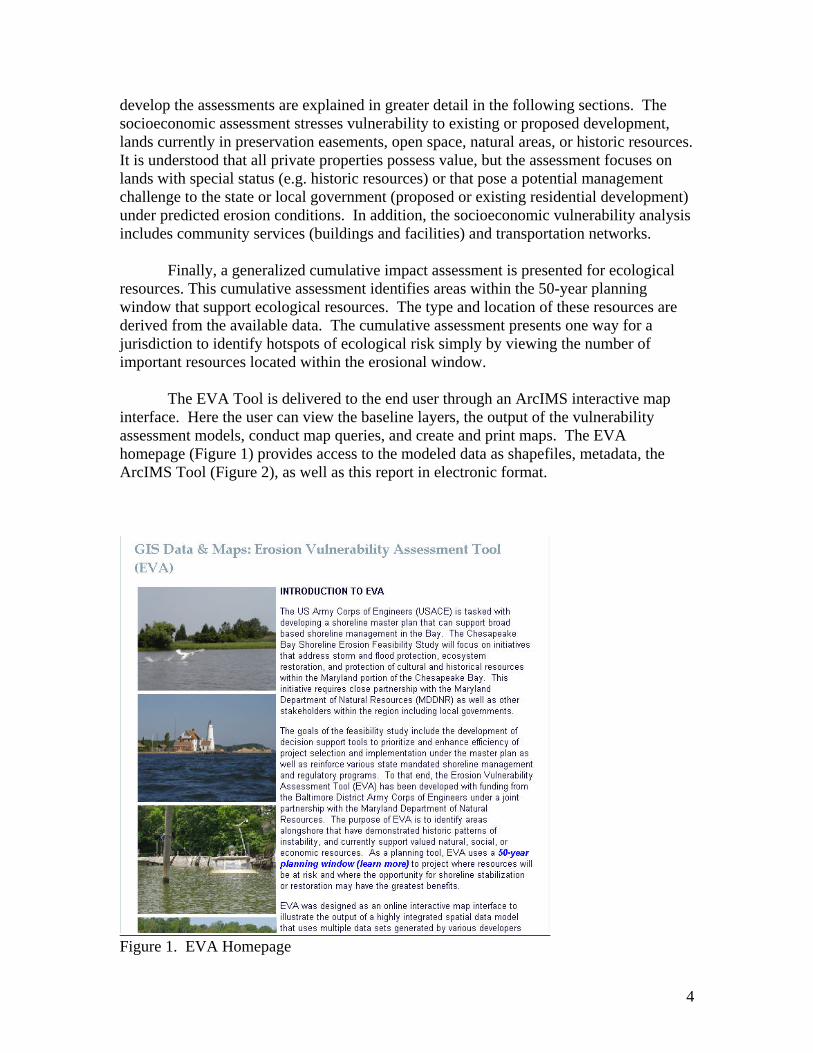
develop the assessments are explained in greater detail in the following sections. The socioeconomic assessment stresses vulnerability to existing or proposed development, lands currently in preservation easements, open space, natural areas, or historic resources. It is understood that all private properties possess value, but the assessment focuses on lands with special status (e.g. historic resources) or that pose a potential management challenge to the state or local government (proposed or existing residential development) under predicted erosion conditions. In addition, the socioeconomic vulnerability analysis includes community services (buildings and facilities) and transportation networks. Finally, a generalized cumulative impact assessment is presented for ecological resources. This cumulative assessment identifies areas within the 50-year planning window that support ecological resources. The type and location of these resources are derived from the available data. The cumulative assessment presents one way for a jurisdiction to identify hotspots of ecological risk simply by viewing the number of important resources located within the erosional window. The EVA Tool is delivered to the end user through an ArcIMS interactive map interface. Here the user can view the baseline layers, the output of the vulnerability assessment models, conduct map queries, and create and print maps. The EVA homepage (Figure 1) provides access to the modeled data as shapefiles, metadata, the ArcIMS Tool (Figure 2), as well as this report in electronic format.

Figure 1. EVA Homepage

4

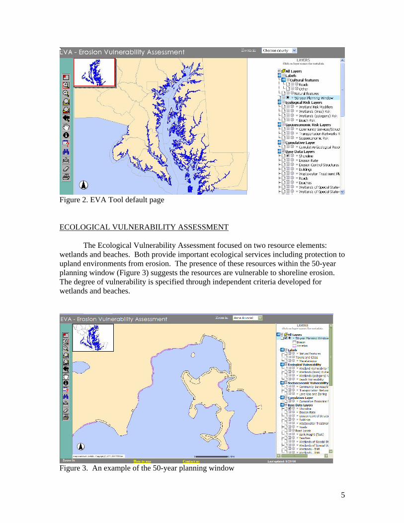
Figure 2. EVA Tool default page ECOLOGICAL VULNERABILITY ASSESSMENT The Ecological Vulnerability Assessment focused on two resource elements: wetlands and beaches. Both provide important ecological services including protection to upland environments from erosion. The presence of these resources within the 50-year planning window (Figure 3) suggests the resources are vulnerable to shoreline erosion. The degree of vulnerability is specified through independent criteria developed for wetlands and beaches.

Figure 3. An example of the 50-year planning window

5

1a. Wetland Vulnerability EVA assigns a vulnerability index to all tidal wetlands mapped by the state of Maryland. The ranking of vulnerability is intended to guide managers to hot spots where restoration or conservation should be considered. Coastal processes responsible for the calculated recession are assumed to continue at the current rate providing the shoreline is not stabilized. That being the case, wetlands (i.e. polygons and arcs) that are completely outside the planning window have a “no risk” factor and are not shown. The data revealed that there are no wetland polygons that are entirely located within the planning window. Given that, the portion of the wetland sitting outside the 50-year planning window is ranked as “low” vulnerability. The area within the 50-year planning window is ranked as “moderate” vulnerability, regardless of the erosion rate. If the wetland is designated by the state of Maryland as a Wetland of Special State Concern (WSSC), the ranking is elevated to “high”. These areas represent the potential loss of “critical” wetland habitat, and are denoted as such because they support or directly provide important ecological services. The higher ranking does not mean the area is undergoing faster erosion. Figure 4 illustrates the vulnerability ranking for wetlands along a stretch of shoreline in Calvert County. The contiguous portion of the wetland (polygon or arc) ranked as “low” vulnerability could be an indicator of the potential for long-term sustainability of a wetland. This approach allows users to project how much of a wetland is likely to remain under the modeled scenario.

Figure 4. Wetland areas ranked low, moderate, and high based on their position relative to the planning window and their special status rating given by the state of Maryland.

6

1b. Modifiers to Wetland Vulnerability

We refer to the ability of a wetland to retreat or migrate landward under natural processes as a long-term mechanism for sustainability. Conditions on the landscape contribute or impede this systematic retreat and in doing so reduce or increase the vulnerability of a wetland to erosion processes. Factors which allow for natural retreat generally include the ability of the wetland to accrete vertically, low lying topography in the riparian upland, absence of development, and no structural controls at the wetland/upland margin. Factors that prevent natural migration and can accelerate the erosion process include development on the upland, presence of erosion control structures, and topographic relief at the shore (bank height >5 feet). We refer to these factors as “modifiers” to the wetland vulnerability.

Inclusion of various modifiers was limited to attributes that have been mapped in

GIS. They include: erosion control structures (offensive and defensive), attributes associated with land use and land cover (e.g. residential development), natural buffers (e.g. beaches) and general riparian topography (bank elevation at the shore). Erosion control structures, beach data, and bank elevation are from the Comprehensive Shoreline Inventory for Maryland. Structure and beach data were first transferred to the revised Maryland Geological Survey’s (MGS) Shoreline, and manually corrected for any spatial discrepancies that exist between the two baselines used. Bank height (as an indicator of riparian topography) was extracted from the Shoreline Inventory database as well, but this attribute was not corrected to the MGS shoreline. The feature was transposed, but based on the combined reported accuracies of the various products, the accuracy of the location may be off by as much as 50 meters. This value is estimated based on accuracy of the original source data. Land use was derived from a 2002 data set provided by the Maryland Department of Planning. A brief discussion below explains the rationale for considering these attributes as a modifier for wetlands vulnerability. EVA does not attempt to modify the vulnerability index assigned to wetland polygons based on the presence or absence of these modifiers. The modifiers are presented as a secondary layer for visual inspection and consideration for users. Erosion control structures built to counter bank erosion problems perhaps have the greatest potential to increase wetland vulnerability. These structures typically provide direct protection to the bank and are generally placed landward of the wetland. Their placement prevents the natural landward horizontal migration of wetlands necessary for wetlands to sustain themselves. For this reason they are viewed to increase the vulnerability of wetlands. Bulkheads, in particular, can generate wave reflection at the structure’s base, undercutting sediment at the base and deepening the shallow water platform. This makes it virtually impossible for a wetland to maintain itself vertically and move horizontally. The result is that the wetland erodes and eventually drowns in place. Structures placed landward of the wetland to defend erosion of the upland bank face include: bulkheads, riprap, or stabilizing walls constructed of miscellaneous or unconventional material, including debris, plastics, and concrete.

7

In contrast, erosion control structures built seaward of the wetland can provide protection from wave energy to both the upland bank and the wetland while still allowing the wetland to migrate landward and maintain its necessary elevation. Structures such as breakwaters fall into this category and are considered beneficial at reducing risk when co-located with wetlands. Land use in the riparian zone often dictates the management of a reach. While all management scenarios cannot be assumed, there is a tendency for managed lands to create impediments or barriers to the inland migration of natural systems like wetlands. These barriers may be erosion control structures, road networks, dwellings, or building complexes. With the high economic investment in such infrastructure, we can assume that property owners will ultimately protect the existing infrastructure and risk the wetland survival. The EVA model, therefore, considers riparian land uses such as commercial, high-density residential, medium-density residential, low-density residential, industrial, institutional, and transportation to reduce the sustainability of any wetland. When found along the shoreline and adjacent to a wetland the model identifies these segments as increasing vulnerability. In contrast to the above, unmanaged lands or those designated as bare ground, beaches, brush, cropland, deciduous forest, evergreen forest, extractive, mixed forest, orchards/vineyards/horticulture, pasture, row and garden crops, water, or wetlands will increase the capacity of the wetland to sustain itself over time. The model does not attempt to predict the likely growth scenarios or land conversions that could occur within the planning period. The Maryland Comprehensive Shoreline Inventory evaluates bank height at the shore using a qualitative assessment method in the field. These data are used to identify topographically low-lying coastal regions. The lowest class in the inventory assessment clusters riparian areas that have observed elevations between zero (0) and five (5) feet. Upper classes include ranges in feet such as 5-10, 10-30, >30. For this study we used the 0-5 feet elevation designation as the cutoff for a modifier that could enhance sustainability of the wetland (i.e. “reduce vulnerability” of wetland loss due to erosion) by allowing for inland migration. Beaches, regardless of land use, will always serve to offer additional natural protection to the marsh and the adjacent upland. On their own and in association with wetlands they are classified as a positive modifier that “reduces vulnerability”. However, land use will most likely have a greater affect on determining the long-term sustainability of the wetland. For this reason, when development is present on the site coincidently with beaches and wetlands, the services provided by the beach can slow the erosion process, but most likely not counter the adverse impacts caused by the upland development. To identify the presence of the conditions described above, a module was generated that queried the various databases for these selected attributes that could “increase” or “reduce” vulnerability. Shoreline segments associated with wetlands were

8

coded based on the presence of those modifying attributes that are coincident with any section of a wetland polygon regardless of its association with the planning window. Within EVA they are highlighted under the layer called Wetland Risk Modifiers as Increases Vulnerability and Decreases Vulnerability (Figure 5). The identify tool must be used to retrieve the attribute table and disclose which modifying attributes are present

Figure 5. Selected areas show where conditions increase wetland vulnerability

Since more than one modifier can co-occur, an ordination of spatial preference was performed with the data that queries all potential modifiers and determines which modifier has the greatest potential to impact a wetland’s risk. The determination is based on best professional judgment. Two examples are offered: 1) an undeveloped site has riprap alongshore, 2) a low lying (<5 feet) bank with residential development. In the first case, an undeveloped site would generally be favorable to a wetland’s long-term sustainability; however, the presence of riprap along the shoreline would work against the benefits of the land use so long as the riprap was maintained. Categorically, the modifier becomes “increases vulnerability”. In the second example, low-lying riparian topography provides the platform necessary for the wetland to migrate inland. Higher bank elevations could provide natural barriers. Development on the upland in low-lying areas is not uncommon. Since protection of the infrastructure is most likely to occur in the future as erosion continues, efforts to maintain the infrastructure in the residential development will reduce the likelihood that the wetland will survive. Therefore, categorically the modifier would be classified as “increases vulnerability” as well. In order to assign the vulnerability, these four layers (bank height, beaches, land use and erosion control structures) were merged with the wetland layer for proper selection and coding.

9

2. Beach Vulnerability EVA assigns a vulnerability factor to all beaches identified in the Comprehensive Shoreline Inventory for Maryland. The classification is based directly on the erosion rates calculated in the revised Maryland Geological Survey’s (MGS) Shoreline Changes study that used historic and current shoreline survey positions to compute changes in position. As mentioned above, this study was revised for EVA to extend into smaller tributaries and to reflect the current state of shoreline hardening in the Bay. The output of the revised shoreline change data can be viewed in the EVA tool by clicking the square next to “Erosion Rates” found under the Base Data Layers. The vulnerability classification applied for beaches is presented in Table 2 and illustrated in Figure 6: Table 2. Vulnerability assessment for beaches Erosion level Average erosion rate Beach VulnerabilitySlight 1 ft/yr Low Low 3 ft/yr Moderate Moderate or High 6 ft/yr or 11 ft/yr High Accretion, No Change or Protected (structure) 0 ft/yr No Risk There are no identifiable modifiers used in this study that increase or decrease a beach’s susceptibility to erosion. The classification applied above acknowledges the potential for structures to protect beaches. The presence of a continuous sediment supply would be required under any scenario to maintain a beach undergoing shoreline erosion. The supply of sediment can be impeded when structures are present. An analysis of this type was beyond the scope of this project.

Figure 6. Beach vulnerability classified here reflects historic erosion rates in Table 2.

10

SOCIOECONOMIC VULNERABILITY ASSESSMENT The Socioeconomic Vulnerability Assessment focuses on societal constituents that comprise community and economic investment. Since individuals and agencies value attributes differently, we chose not to rank or order shoreline segments at the risk of generating a planning tool that was restrictive in its utility. Therefore, the risk analysis for socioeconomic resources merely identifies where the resources intersect the 50-year planning window. The anticipated expectation is that these resources may be severely compromised in the coming years due to erosion. In this version of EVA, there is no attempt to quantify the economic loss associated with any particular resource. To develop the socioeconomic vulnerability assessment, various external datasets are combined into three major socioeconomic categories: Land use and Zoning which principally addresses land use, land cover, and zoning; Community Services and Structures focuses on specific facilities such as wastewater treatment plants; and Transportation Networks which includes primary, secondary and tertiary roads. Within the EVA Tool, these are represented as separate layers under the heading Socioeconomic Vulnerability Layers. Planners also can use the 50-year planning window as a planning tool to guide proposed activity in the riparian zone. As counties plan for future scenarios they will consider the preservation of waterfront districts as well as ecological services. EVA provides the opportunity to identify where uplands are best suited for long term wetland preservation versus more suited toward expansion of existing waterfront developments and services. 1. Socioeconomic Vulnerability The Socioeconomic Vulnerability layer combines the following datasets: land use data derived from 2002 land cover; zoning data compiled by the State from information provided by the localities; public lands data; conservation easements; and historic resources. Data were organized into simplified land classes: agriculture, developed, and open space/natural areas. Agriculture, derived from the land use data layer clusters crop and pasture land. The Open space/Natural areas class includes data layers from sources that encompass county parks, private conservation properties, forest legacy easements, MD environmental trust easements, and land use corresponding to open space and natural areas, such as forest and bare ground, among others. Developed infrastructure includes historic resources (MD inventory of historic properties, MD historic trust easements, National Register of historic places), general zoning, as well as land use defined as commercial, industrial, institutional, low-density residential, medium-density residential, high-density residential, and transportation. Users who desire more specific information can use the identify tool to retrieve the original attribute information for each polygon.

11

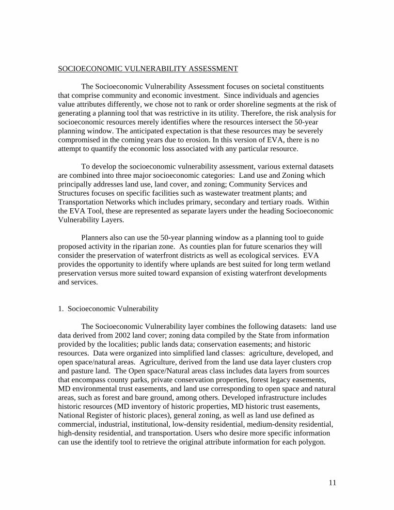
EVA classifies the portion of a polygon that resides within the planning window as “vulnerable” (Figure 7). Large areas of a polygon can lie outside the zone of vulnerability but are not classified or shown. Using color symbology the tool distinguishes the type of land use within the area of the planning window. To view the extent of these areas outside the planning window the user needs to view the base layers. The identification of these land uses located within zones vulnerable to erosion can help to prioritize coastal restoration projects, identify possible areas for conservation, and provide planning and zoning guidance to expanding waterfront communities.

Figure 7. Land Use and Zoning illustrated within the planning window. 2. Community Services/Structures The Community Services/Structures layer identifies features necessary for community living that are within the 50-year planning window. The attributes or features considered in this assessment are driven by the available data received through state offices. They include: buildings (fire stations, hospitals, police stations, and schools) and wastewater treatment plants (municipal and industrial). The identify tool must be used to retrieve specific information about the individual building or facility. Any structure present within the window is perceived to carry some risk. Structures within 10 meters of the planning window also are recognized as being “potentially at risk”. Figure 8 illustrates two wastewater treatment facilities located in Anne Arundel County that fall within the 50-year planning window. EVA presents an opportunity for local governments or state agencies to determine whether the risk is significant enough to consider protection strategies.

12

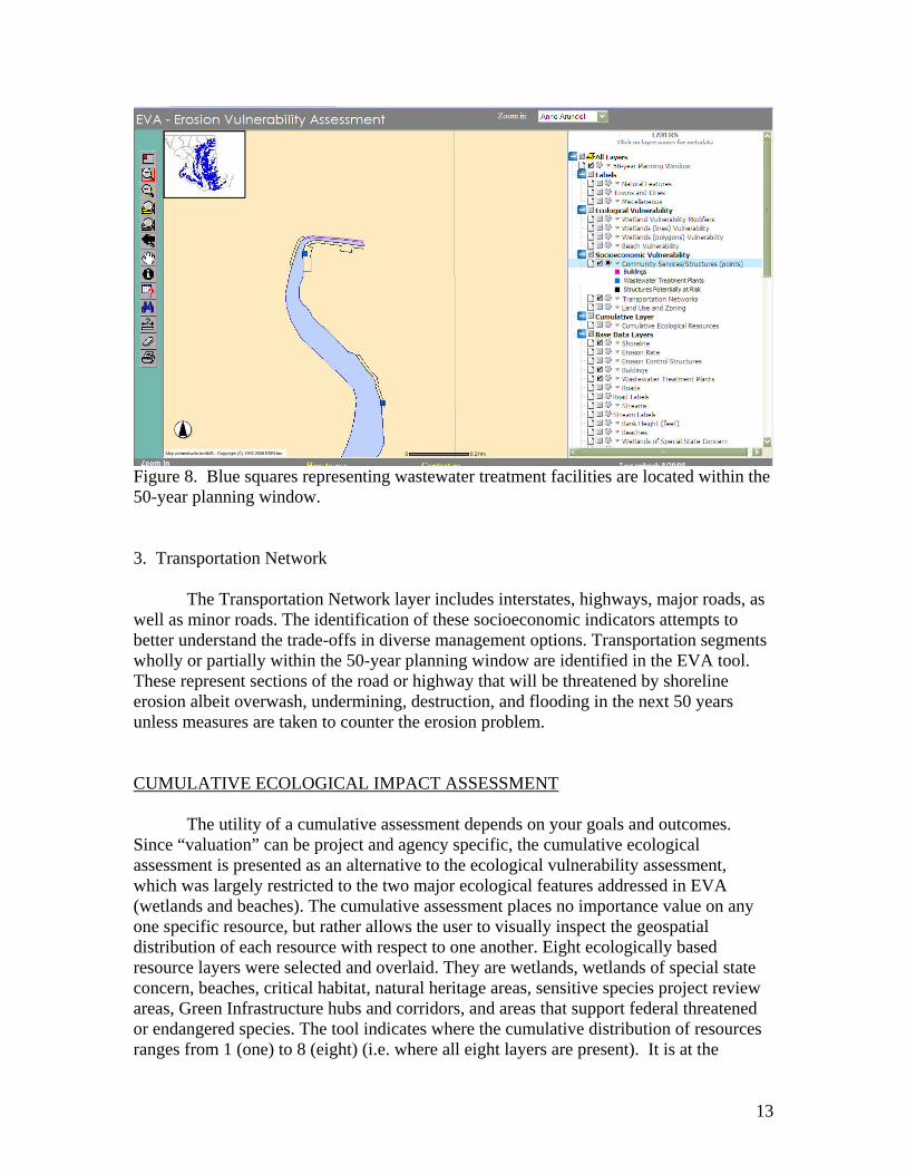
Figure 8. Blue squares representing wastewater treatment facilities are located within the 50-year planning window. 3. Transportation Network The Transportation Network layer includes interstates, highways, major roads, as well as minor roads. The identification of these socioeconomic indicators attempts to better understand the trade-offs in diverse management options. Transportation segments wholly or partially within the 50-year planning window are identified in the EVA tool. These represent sections of the road or highway that will be threatened by shoreline erosion albeit overwash, undermining, destruction, and flooding in the next 50 years unless measures are taken to counter the erosion problem. CUMULATIVE ECOLOGICAL IMPACT ASSESSMENT The utility of a cumulative assessment depends on your goals and outcomes. Since “valuation” can be project and agency specific, the cumulative ecological assessment is presented as an alternative to the ecological vulnerability assessment, which was largely restricted to the two major ecological features addressed in EVA (wetlands and beaches). The cumulative assessment places no importance value on any one specific resource, but rather allows the user to visually inspect the geospatial distribution of each resource with respect to one another. Eight ecologically based resource layers were selected and overlaid. They are wetlands, wetlands of special state concern, beaches, critical habitat, natural heritage areas, sensitive species project review areas, Green Infrastructure hubs and corridors, and areas that support federal threatened or endangered species. The tool indicates where the cumulative distribution of resources ranges from 1 (one) to 8 (eight) (i.e. where all eight layers are present). It is at the

13

discretion of the user to decide whether the combination of resources present is more or less significant. This may have an impact on how a government manages these areas. EVA illustrates the cumulative assessment using color-coded symbology (1-8). Using the identify tool a pop-up window displays the attribute table to list more information regarding the type of resource(s) present. Figure 9 shows an area where the cumulative resources range from 2-6. From a selected polygon, the attribute table reveals the selected polygon is a wetland of special state concern (WSSC) and supports some federally listed rare, threatened, or endangered species. The wetland is also part of the state’s Greenway network of conservation hubs and corridors.

Figure 9. Zones of cumulative ecological resources within the planning window are mapped. The attribute table is revealed for a selected polygon when the Identify Tool “i” in the tool menu on the left is selected and the layer is made active by highlighting the circle next to the checked box in the legend.

14

A WORD ABOUT SCALE All projects that bring together multiple data layers from different sources are challenged by spatial and temporal scales. This project is no different. In the coastal environment, this is most evident when comparing data originally referenced to different shoreline bases and mapped at different scales. Efforts to correct data to a single baseline can consume resources. Early in this project the decision was made to identify the most recent MGS shoreline as the project’s baseline since EVA was so tightly linked to the planning window, which was generated from this baseline data. Nevertheless, many other data used in the project are referenced to other baselines. Some of those have been corrected; others have not. One of the obvious visual and analytical drawbacks to this issue is the apparent loss of logical topology. Examples of this include upland land use classes and features that appear seaward of the shoreline. If you are surprised to see a road extending into the water, don’t be. Problems that have a major affect on the project outcome have been corrected. Others have been left for the observer to recognize. In most cases, these datasets are so familiar to the end users that this is seen as commonplace. The integration of the 2002 Land Use from thematic mapper imagery is a perfect example. Consider the scale in displaying and using the vectors. Displaying the vectors at scales larger than those of the source documents is considered bad practice. TECHNOLOGY ArcGIS 9.2 was used for all geoprocessing steps necessary to generate the products delivered in the EVA tool. The EVA tool is served on a Gateway E-9510T Server running Apache 2.0 web server. Microsoft SQL Server 2005 and ArcSDE 9.2 manage the database. WEBSITE http://ccrm.vims.edu/gis_data_maps/interactive_maps/erosion_vulnerability/index.html REFERENCES Danforth, W.W., and Thieler, E.R., 1992, Digital Shoreline Analysis System (DSAS) User’s Guide, Version 1.0: U.S. Geological Survey Open-File Report 92-355, 18 p. Hennessee, L., Valentino, M.J., and Lesh, A.M., 2003, Determining shoreline erosion rates for coastal regions of Maryland (Part 2): Coastal and Estuarine Geology File Report No. 03-01, Maryland Geological Survey, Baltimore, MD., 53 p. Center for Coastal Resources Management, 2004. Maryland Comprehensive Shoreline Inventory, http://ccrm.vims.edu/gis_data_maps/shoreline_inventories/index.html, Virginia Institute of Marine Science, College of William and Mary, Gloucester Point, VA.

15

16

Appendix 1. Baseline Data Ecological Vulnerability was determined using data extracted from the following GIS layers: Beaches Erosion Control Structures Land Use - 2002 MD Department of Natural Resources Wetlands Wetlands of Special State Concern (WSSC) Critical Habitat Natural Heritage Areas Sensitive Species Project Review Areas Federal Threatened and Endangered Species Green Infrastructure hubs and corridors Riparian bank height Socioeconomic risk was determined using data extracted from the following GIS layers: Land Use – 2002 General Zoning County Parks Private Conservation Properties Forest Legacy Easements MD Environmental Trust Easements MD Inventory of Historic Properties MD Historic Trust Easements National Register of Historic Places Roads Buildings Wastewater Treatment Plants Other Layers of interest: Boat wake erosion zones Streams Floodplains Shoreline Designated No-Wake Zones Municipalities Enterprise Zones Designated Neighborhoods County Boundaries Feature Labels