Erosion in slug flow - University of · PDF fileEROSION IN SLUG FLOW November 2011 ... is...
25
EROSION IN SLUG FLOW November 2011 Solid Particle Erosion in Slug Flow Introduction Sand produced by oil and gas producers creates many problems such as accumulation of the sand in perforation tunnels, lines and pumps; damage to production equipment, well tubing and fittings as well as inside walls of the reservoir. Sand screens or gravel packs are commonly installed in open hole well bores to avoid the passage of sand along with the reservoir fluids. However, this sand control approach may fail due to plugging of the screens with smaller particles causing an increase in the local fluid velocity at other portions of the screen causing damage. This process allows sand production, where this sand repeatedly impacts pipe walls removing material gradually. The mechanism of material loss depends on the type of pipe wall material. For example, the erosion in ductile materials is caused by the localized pipe wall deformation resulting in cutting action caused by severe particle impacts. Other types of failure mechanisms include ploughing, fatigue and the brittle fracture. Prediction of solid particle erosion is extremely difficult because of its dependence on many factors. The important ones are flow pattern, sand distribution, flow geometry, fluid flow rates and particle properties such as size and shape. The complexity of erosion is increased in multiphase flow because of the different flow patterns that occur under different operating conditions. These different flow patterns affect the sand particle impact characteristics and cause different amounts of erosion. The geometries which are more susceptible to erosion are the ones which change the flow direction such as elbows, Tee joints, and sudden expansion and contraction zones. Since erosion depends on multiple factors, developing a predictive tool for erosion is a challenging task. The severity of erosion can be clearly emphasized by the pictures shown below. Figure 1 shows the locations of pipe failures caused by erosion in a stainless steel pipe at two different bends. This location of failure supports the statement already made that erosion failures commonly occur in a locations where the flow direction changes. These failures were observed after conducting experiments in a laboratory setting for a period intermittently of 3 months.
Transcript of Erosion in slug flow - University of · PDF fileEROSION IN SLUG FLOW November 2011 ... is...

EROSION IN SLUG FLOW
November 2011
Solid Particle Erosion in Slug Flow
Introduction
Sand produced by oil and gas producers creates many problems such as accumulation of
the sand in perforation tunnels, lines and pumps; damage to production equipment, well tubing
and fittings as well as inside walls of the reservoir. Sand screens or gravel packs are commonly
installed in open hole well bores to avoid the passage of sand along with the reservoir fluids.
However, this sand control approach may fail due to plugging of the screens with smaller
particles causing an increase in the local fluid velocity at other portions of the screen causing
damage. This process allows sand production, where this sand repeatedly impacts pipe walls
removing material gradually. The mechanism of material loss depends on the type of pipe wall
material. For example, the erosion in ductile materials is caused by the localized pipe wall
deformation resulting in cutting action caused by severe particle impacts. Other types of failure
mechanisms include ploughing, fatigue and the brittle fracture. Prediction of solid particle
erosion is extremely difficult because of its dependence on many factors. The important ones are
flow pattern, sand distribution, flow geometry, fluid flow rates and particle properties such as
size and shape. The complexity of erosion is increased in multiphase flow because of the
different flow patterns that occur under different operating conditions. These different flow
patterns affect the sand particle impact characteristics and cause different amounts of erosion.
The geometries which are more susceptible to erosion are the ones which change the flow
direction such as elbows, Tee joints, and sudden expansion and contraction zones. Since erosion
depends on multiple factors, developing a predictive tool for erosion is a challenging task.
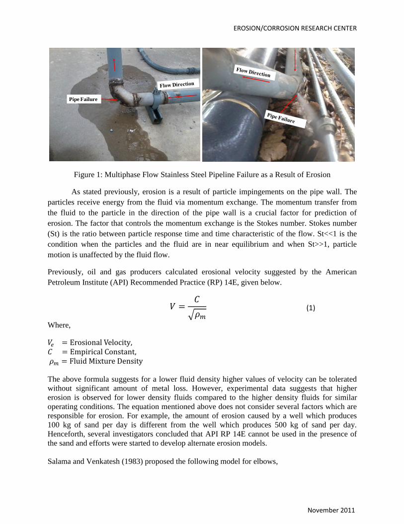
The severity of erosion can be clearly emphasized by the pictures shown below. Figure 1
shows the locations of pipe failures caused by erosion in a stainless steel pipe at two different
bends. This location of failure supports the statement already made that erosion failures
commonly occur in a locations where the flow direction changes. These failures were observed
after conducting experiments in a laboratory setting for a period intermittently of 3 months.
EROSION/CORROSION RESEARCH CENTER
November 2011
Figure 1: Multiphase Flow Stainless Steel Pipeline Failure as a Result of Erosion
As stated previously, erosion is a result of particle impingements on the pipe wall. The
particles receive energy from the fluid via momentum exchange. The momentum transfer from
the fluid to the particle in the direction of the pipe wall is a crucial factor for prediction of
erosion. The factor that controls the momentum exchange is the Stokes number. Stokes number
(St) is the ratio between particle response time and time characteristic of the flow. St<<1 is the
condition when the particles and the fluid are in near equilibrium and when St>>1, particle
motion is unaffected by the fluid flow.
Previously, oil and gas producers calculated erosional velocity suggested by the American
Petroleum Institute (API) Recommended Practice (RP) 14E, given below.
(1)
Where,
The above formula suggests for a lower fluid density higher values of velocity can be tolerated
without significant amount of metal loss. However, experimental data suggests that higher
erosion is observed for lower density fluids compared to the higher density fluids for similar
operating conditions. The equation mentioned above does not consider several factors which are
responsible for erosion. For example, the amount of erosion caused by a well which produces
100 kg of sand per day is different from the well which produces 500 kg of sand per day.
Henceforth, several investigators concluded that API RP 14E cannot be used in the presence of
the sand and efforts were started to develop alternate erosion models.
Salama and Venkatesh (1983) proposed the following model for elbows,
Pipe Failure
EROSION IN SLUG FLOW
November 2011
(2)
Where,
, P = Material Hardness (psi)
Salama and Ventakesh assumed the particle impact velocity to be equal to the fluid velocity. This
is a good assumption for lower density fluids but not for the higher density fluids. Bourgoyne
(1989) conducted many erosion experiments and developed an empirical relation for
erosionshown below
(3)
Where,
H = Wall thickness (m),
,
,
,
,
,
Fe = Empirical Constant
The above equation is clearly not general. It is valid only under the conditions where Bourgoyne
conducted experiments. Moreover, he did not consider the influence of flow-pattern and particle
size on erosion.
Shirazi et al. (1995) developed a stagnation length concept to develop a more generalized
model for erosion. Using the stagnation length concept, they predicted particle impact velocity as
it is the most crucial parameter for the erosion calculations. Stagnation length is a distance away
from the wall where the particle velocity component in the direction of the wall begins to reduce.
For single-phase flow, the particle velocity upon entering the stagnation zone is assumed to be
the average fluid velocity. Also, the average fluid velocity is assumed to vary linearly in the
stagnation length to achieve zero velocity at the wall (no slip boundary condition). The particle
velocity at the wall is calculated by dividing the stagnation length into many increments and
solving the force balance. The force assumed to be acting on the particle is just the drag force. In
this concept, radial forces acting on the particle due to turbulence were not considered; therefore
the particle is forced to travel only in one direction, and so this approach is called the 1-
EROSION/CORROSION RESEARCH CENTER
November 2011
Dimensional (1-D) approach. This approach under predicts the erosion magnitudes for smaller
particles. To overcome the drawbacks of the 1-D approach, researchers at E/CRC have
developed a 2-Dimensional (2-D) approach.
Objectives
The objective of the current study is to use a state-of-the art Ultrasonic Testing (UT) to
collect erosion data and compare with data collected using Electrical Resistance (ER) probes.
Ultrasonic Testing for Measuring Erosion
A standard 3-inch elbow has been equipped with 16 transducers at different locations
mounted on the elbow. This enables the erosion pattern under different operating conditions to
be determined. The background of the ultrasonic testing and the major components is explained
in detail below.
Ultrasonic Testing (UT) utilizes high frequency sound energy that is used in many industries for
flaw detection, thickness measurements, and material characterization. The basic components of
UT are the pulsar/receiver, transducers, a multiplexer, a digitizer and the display devices.
“Pulsar” is an electronic device capable of generating high voltage electrical pulses. Powered by
these pulses, the transducer will generate the ultrasonic energy which travels into the material
until it locates a discontinuity. Once the sound wave reaches the discontinuity, most of its energy
is reflected back to the transducer which converts that energy to an electrical signal for analysis.
The frequency of the transducers used for the current study is 10 MHz. This transducer
frequency is very powerful and is the frequency used commonly in medical diagnostics.
Increasing the frequency of the transducer results in better resolution and lower wavelengths.
Another component of UT is the multiplexer, which is a multichannel switch that enables the
user to select the transducer to receive the excitation pulse. A final important component is the
digitizer which converts the analogue signal received by the transducer into the digital output for
further analysis.
The size of the transducers used in this work (approximately ¼ inch) enables a relatively
high sensor density on the outside of the elbow. The high sensor density allows thickness
measurements at multiple locations on the bend. Also, the technique is non-destructive, not
disturbing the flow inside the elbow. The ultrasonic wave speed inside the elbow is linear in the
normal temperature range, so the thickness can be compensated for the temperature
mathematically. The thickness of the pipe wall at the location of interest can be determined by
multiplying the velocity of the sound wave in that particular material and the time required to
travel through that thickness. Two techniques are available for measuring the time of travel
inside the thickness and those are known as through transmission and the pulse/echo methods. In
the through transmission method, there are two transducers; one generates the ultrasound wave
inside the material and the other is mounted on the other side of the sample of interest to detect
the arrival of the ultrasound wave. Whereas in the pulse/echo method, a single transducer
contains two elements, one element is responsible for the generation of the ultrasound wave,
EROSION IN SLUG FLOW
November 2011
whereas the other one is accountable for the detection of the arrival of ultrasound wave. These
transducers which perform the dual role of sending and receiving are called the dual element
transducers. In the present study, the pulse/echo technique is implemented and therefore dual
element transducers are used.
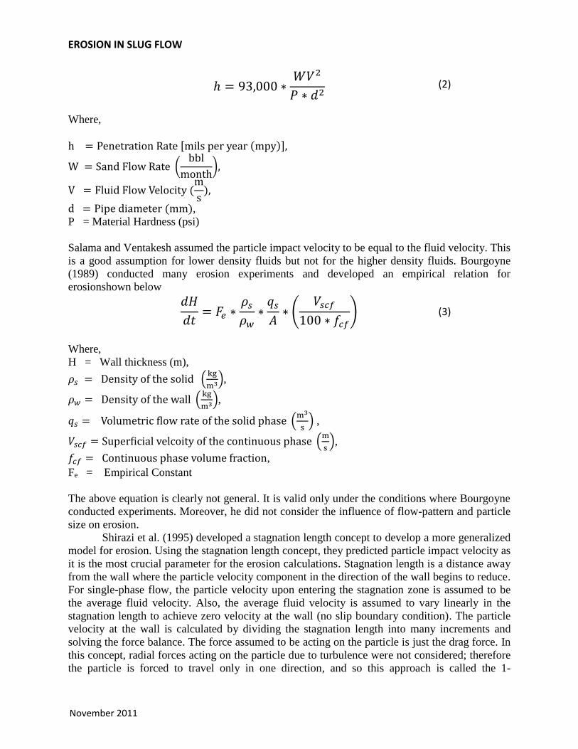
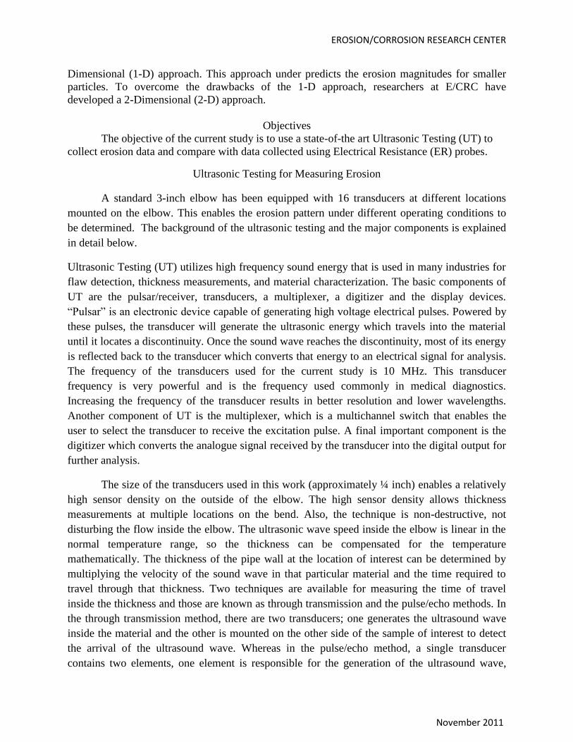
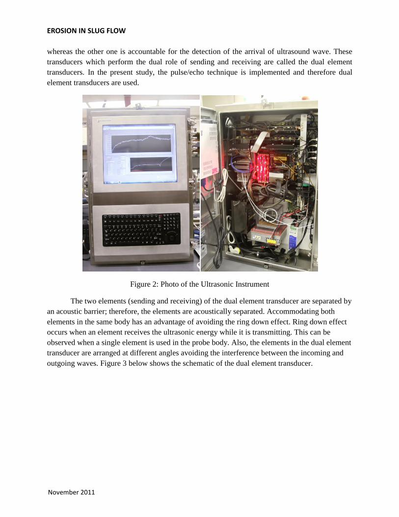
Figure 2: Photo of the Ultrasonic Instrument
The two elements (sending and receiving) of the dual element transducer are separated by
an acoustic barrier; therefore, the elements are acoustically separated. Accommodating both
elements in the same body has an advantage of avoiding the ring down effect. Ring down effect
occurs when an element receives the ultrasonic energy while it is transmitting. This can be
observed when a single element is used in the probe body. Also, the elements in the dual element
transducer are arranged at different angles avoiding the interference between the incoming and
outgoing waves. Figure 3 below shows the schematic of the dual element transducer.
EROSION/CORROSION RESEARCH CENTER
November 2011
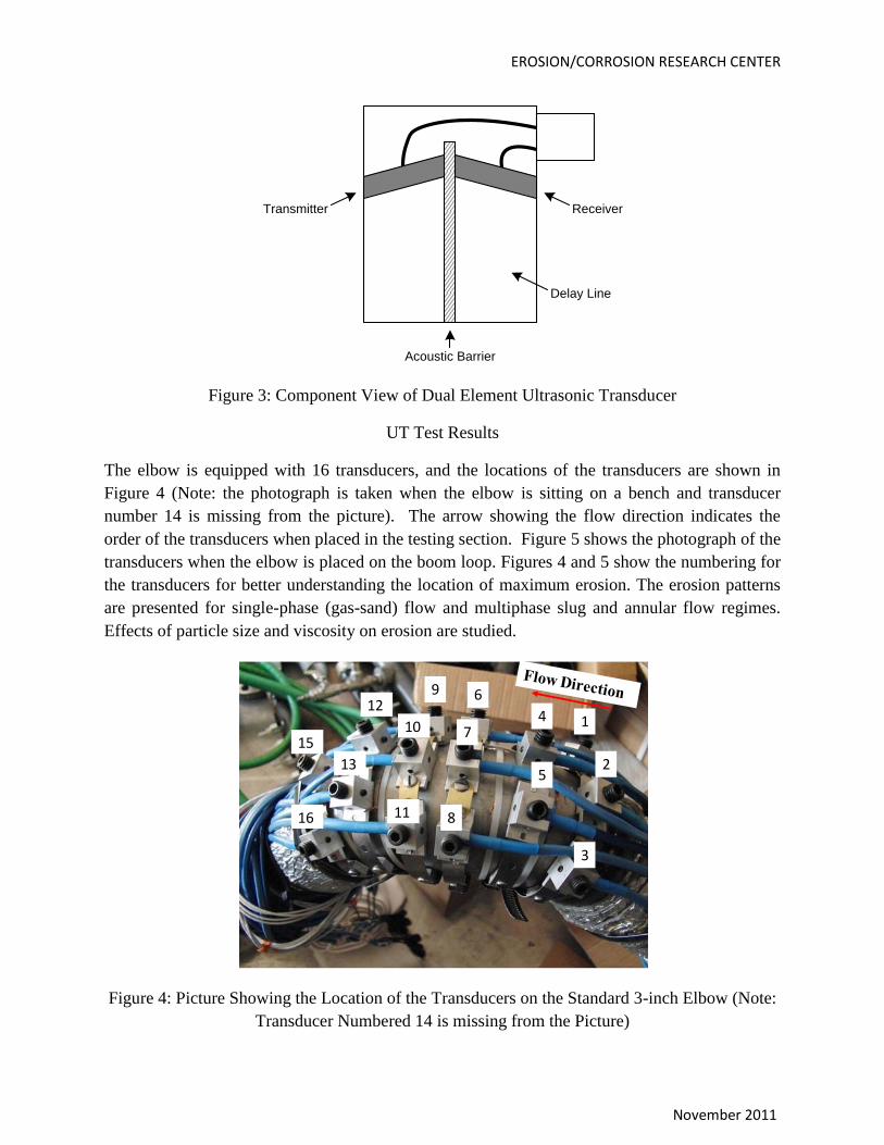
Figure 3: Component View of Dual Element Ultrasonic Transducer
UT Test Results
The elbow is equipped with 16 transducers, and the locations of the transducers are shown in
Figure 4 (Note: the photograph is taken when the elbow is sitting on a bench and transducer
number 14 is missing from the picture). The arrow showing the flow direction indicates the
order of the transducers when placed in the testing section. Figure 5 shows the photograph of the
transducers when the elbow is placed on the boom loop. Figures 4 and 5 show the numbering for
the transducers for better understanding the location of maximum erosion. The erosion patterns
are presented for single-phase (gas-sand) flow and multiphase slug and annular flow regimes.
Effects of particle size and viscosity on erosion are studied.
Figure 4: Picture Showing the Location of the Transducers on the Standard 3-inch Elbow (Note:
Transducer Numbered 14 is missing from the Picture)
Transmitter Receiver
Acoustic Barrier
Delay Line
14
8
9
10 7
11
13
126
5
3
16
15
2
EROSION IN SLUG FLOW
November 2011
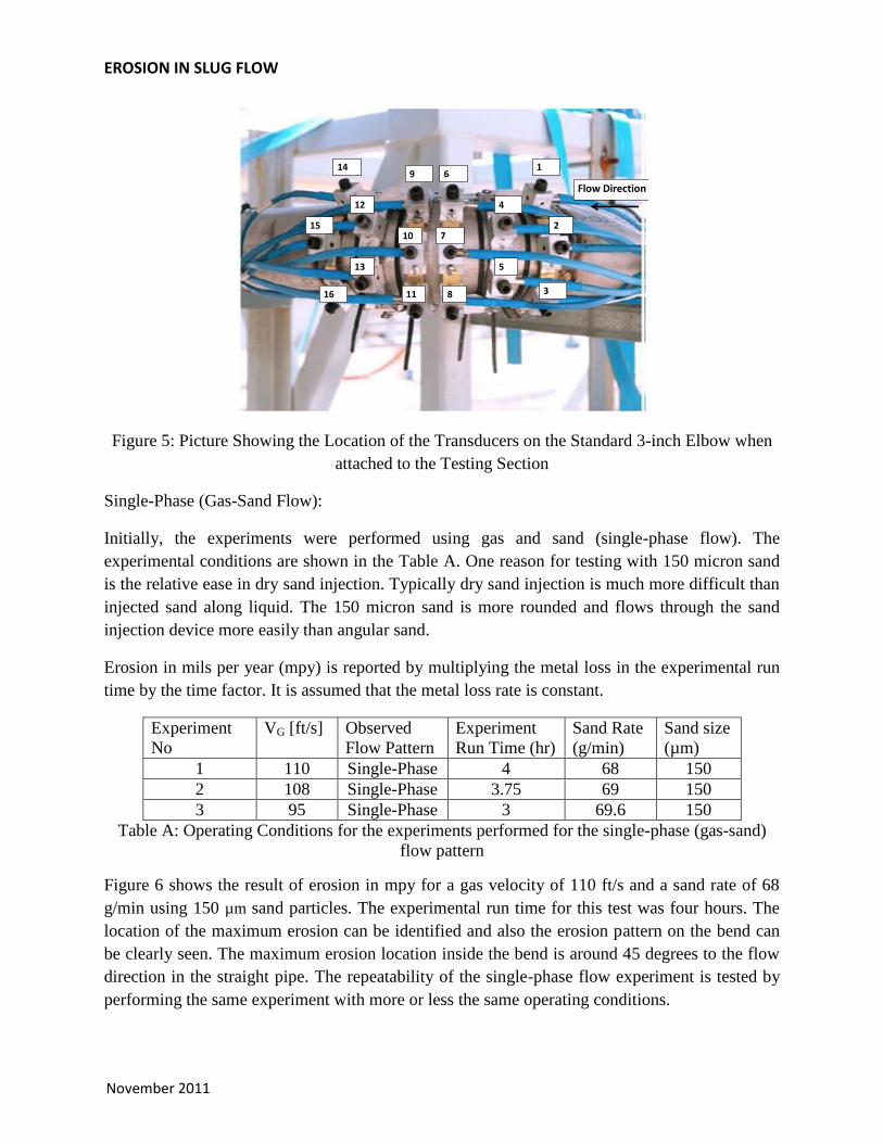
Figure 5: Picture Showing the Location of the Transducers on the Standard 3-inch Elbow when
attached to the Testing Section
Single-Phase (Gas-Sand Flow):
Initially, the experiments were performed using gas and sand (single-phase flow). The
experimental conditions are shown in the Table A. One reason for testing with 150 micron sand
is the relative ease in dry sand injection. Typically dry sand injection is much more difficult than
injected sand along liquid. The 150 micron sand is more rounded and flows through the sand
injection device more easily than angular sand.
Erosion in mils per year (mpy) is reported by multiplying the metal loss in the experimental run
time by the time factor. It is assumed that the metal loss rate is constant.
Experiment
No
VG [ft/s] Observed
Flow Pattern
Experiment
Run Time (hr)
Sand Rate
(g/min)
Sand size
(µm)
1 110 Single-Phase 4 68 150
2 108 Single-Phase 3.75 69 150
3 95 Single-Phase 3 69.6 150
Table A: Operating Conditions for the experiments performed for the single-phase (gas-sand)
flow pattern
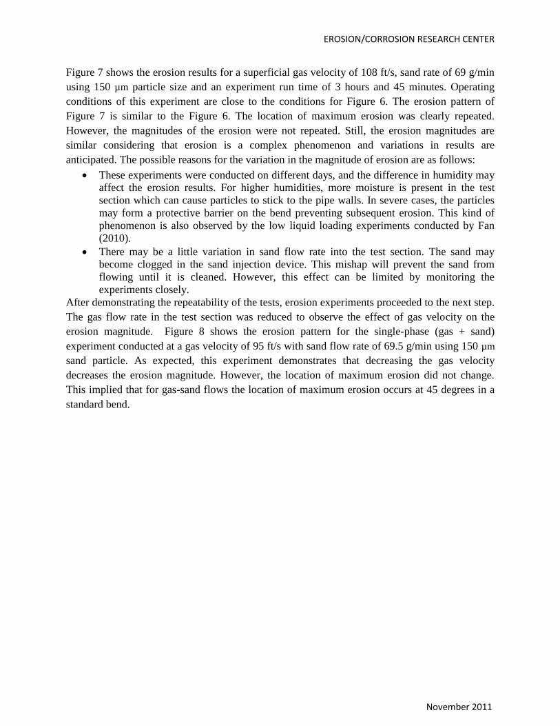
Figure 6 shows the result of erosion in mpy for a gas velocity of 110 ft/s and a sand rate of 68
g/min using 150 µm sand particles. The experimental run time for this test was four hours. The
location of the maximum erosion can be identified and also the erosion pattern on the bend can
be clearly seen. The maximum erosion location inside the bend is around 45 degrees to the flow
direction in the straight pipe. The repeatability of the single-phase flow experiment is tested by
performing the same experiment with more or less the same operating conditions.
5
Flow Direction
1
2
3
4
5
6
7
8
9
10
11
12
13
14
15
16
EROSION/CORROSION RESEARCH CENTER
November 2011
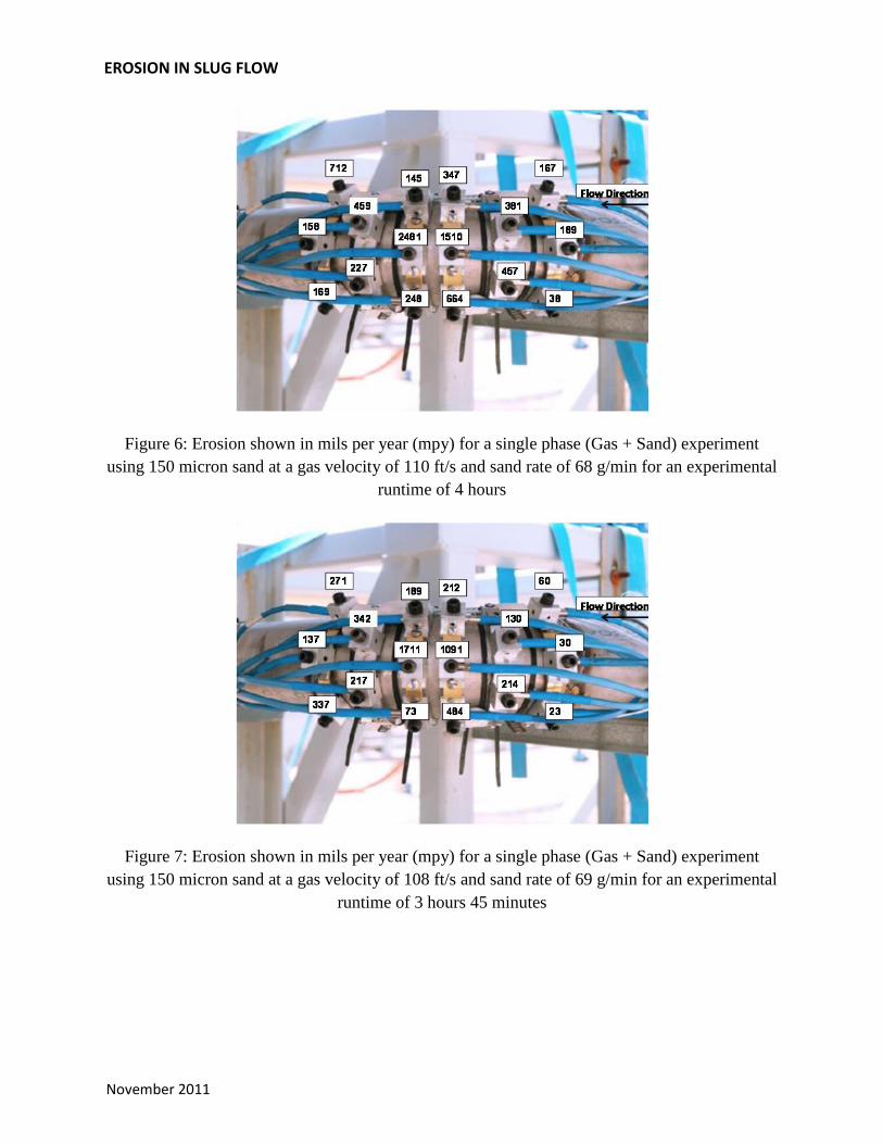
Figure 7 shows the erosion results for a superficial gas velocity of 108 ft/s, sand rate of 69 g/min
using 150 µm particle size and an experiment run time of 3 hours and 45 minutes. Operating
conditions of this experiment are close to the conditions for Figure 6. The erosion pattern of
Figure 7 is similar to the Figure 6. The location of maximum erosion was clearly repeated.
However, the magnitudes of the erosion were not repeated. Still, the erosion magnitudes are
similar considering that erosion is a complex phenomenon and variations in results are
anticipated. The possible reasons for the variation in the magnitude of erosion are as follows:
These experiments were conducted on different days, and the difference in humidity may
affect the erosion results. For higher humidities, more moisture is present in the test
section which can cause particles to stick to the pipe walls. In severe cases, the particles
may form a protective barrier on the bend preventing subsequent erosion. This kind of
phenomenon is also observed by the low liquid loading experiments conducted by Fan
(2010).
There may be a little variation in sand flow rate into the test section. The sand may
become clogged in the sand injection device. This mishap will prevent the sand from
flowing until it is cleaned. However, this effect can be limited by monitoring the
experiments closely.
After demonstrating the repeatability of the tests, erosion experiments proceeded to the next step.
The gas flow rate in the test section was reduced to observe the effect of gas velocity on the
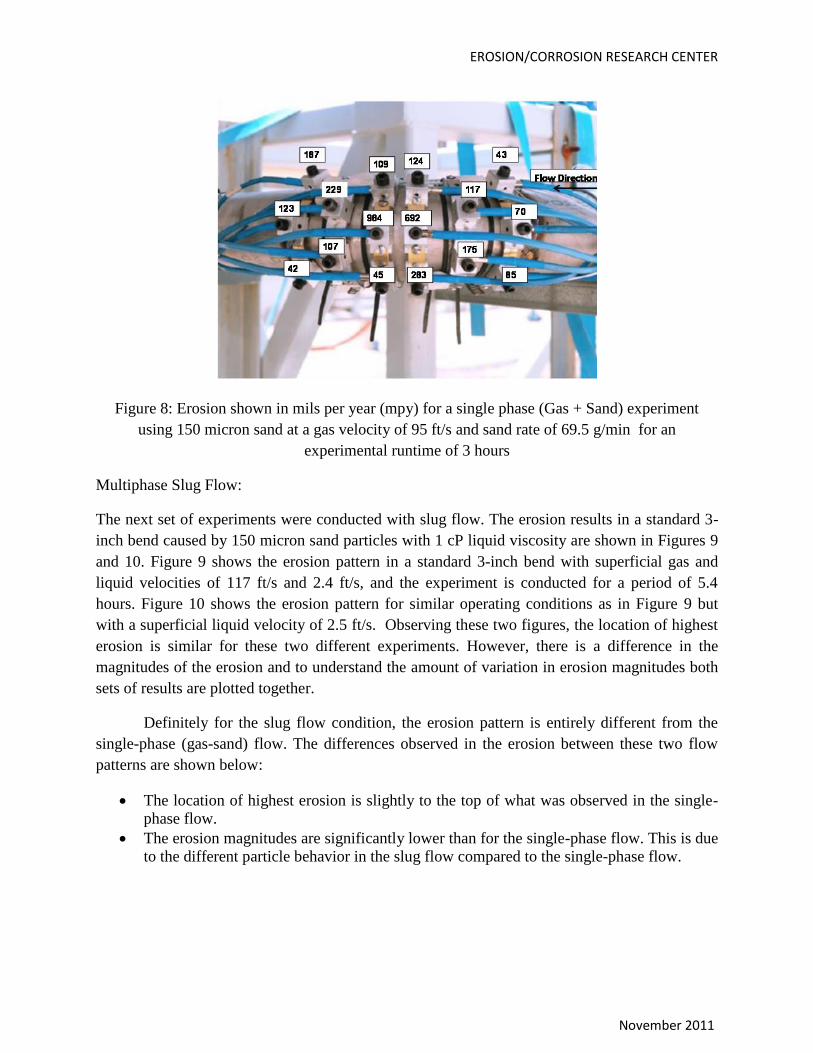
erosion magnitude. Figure 8 shows the erosion pattern for the single-phase (gas + sand)
experiment conducted at a gas velocity of 95 ft/s with sand flow rate of 69.5 g/min using 150 µm
sand particle. As expected, this experiment demonstrates that decreasing the gas velocity
decreases the erosion magnitude. However, the location of maximum erosion did not change.
This implied that for gas-sand flows the location of maximum erosion occurs at 45 degrees in a
standard bend.
EROSION IN SLUG FLOW
November 2011
Figure 6: Erosion shown in mils per year (mpy) for a single phase (Gas + Sand) experiment
using 150 micron sand at a gas velocity of 110 ft/s and sand rate of 68 g/min for an experimental
runtime of 4 hours
Figure 7: Erosion shown in mils per year (mpy) for a single phase (Gas + Sand) experiment
using 150 micron sand at a gas velocity of 108 ft/s and sand rate of 69 g/min for an experimental
runtime of 3 hours 45 minutes
EROSION/CORROSION RESEARCH CENTER
November 2011
Figure 8: Erosion shown in mils per year (mpy) for a single phase (Gas + Sand) experiment
using 150 micron sand at a gas velocity of 95 ft/s and sand rate of 69.5 g/min for an
experimental runtime of 3 hours
Multiphase Slug Flow:
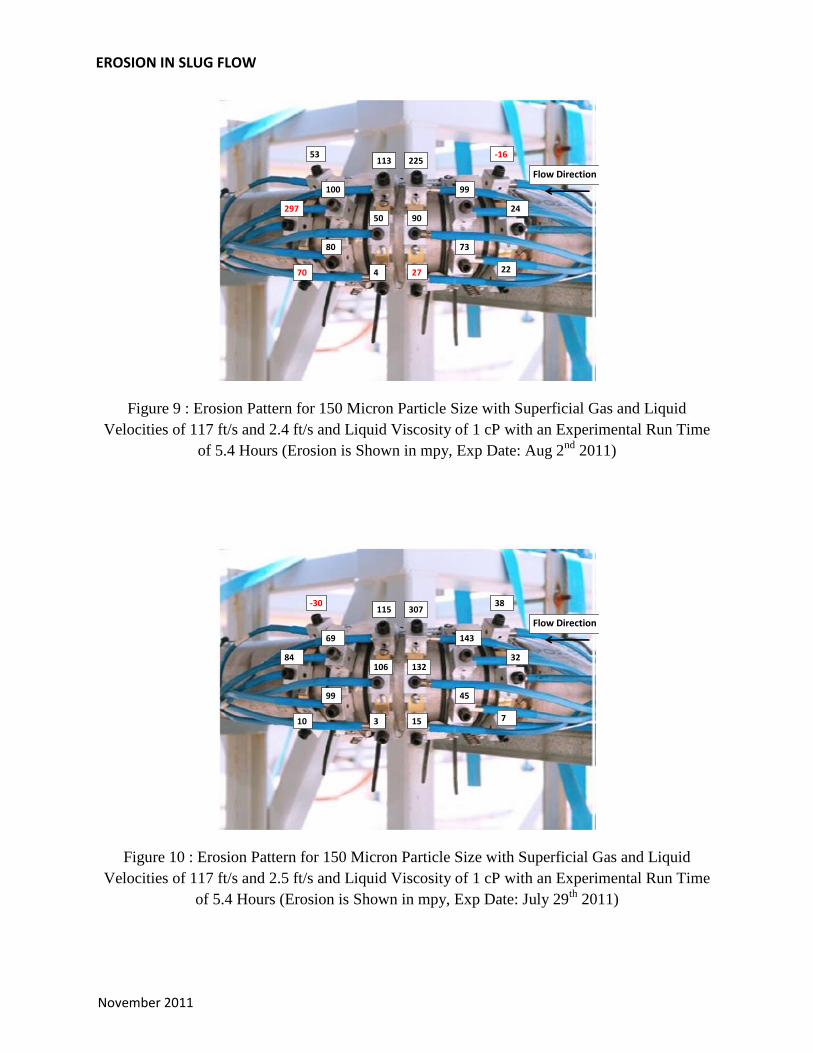
The next set of experiments were conducted with slug flow. The erosion results in a standard 3-
inch bend caused by 150 micron sand particles with 1 cP liquid viscosity are shown in Figures 9
and 10. Figure 9 shows the erosion pattern in a standard 3-inch bend with superficial gas and
liquid velocities of 117 ft/s and 2.4 ft/s, and the experiment is conducted for a period of 5.4
hours. Figure 10 shows the erosion pattern for similar operating conditions as in Figure 9 but
with a superficial liquid velocity of 2.5 ft/s. Observing these two figures, the location of highest
erosion is similar for these two different experiments. However, there is a difference in the
magnitudes of the erosion and to understand the amount of variation in erosion magnitudes both
sets of results are plotted together.
Definitely for the slug flow condition, the erosion pattern is entirely different from the
single-phase (gas-sand) flow. The differences observed in the erosion between these two flow
patterns are shown below:
The location of highest erosion is slightly to the top of what was observed in the single-
phase flow.
The erosion magnitudes are significantly lower than for the single-phase flow. This is due
to the different particle behavior in the slug flow compared to the single-phase flow.
EROSION IN SLUG FLOW
November 2011
Figure 9 : Erosion Pattern for 150 Micron Particle Size with Superficial Gas and Liquid
Velocities of 117 ft/s and 2.4 ft/s and Liquid Viscosity of 1 cP with an Experimental Run Time
of 5.4 Hours (Erosion is Shown in mpy, Exp Date: Aug 2nd
2011)
Figure 10 : Erosion Pattern for 150 Micron Particle Size with Superficial Gas and Liquid
Velocities of 117 ft/s and 2.5 ft/s and Liquid Viscosity of 1 cP with an Experimental Run Time
of 5.4 Hours (Erosion is Shown in mpy, Exp Date: July 29th
2011)
Flow Direction
-16
24
22
99
73
225
90
27
113
50
4
100
80
53
297
70
Flow Direction
38
32
7
143
45
307
132
15
115
106
3
69
99
-30
84
10
EROSION/CORROSION RESEARCH CENTER
November 2011
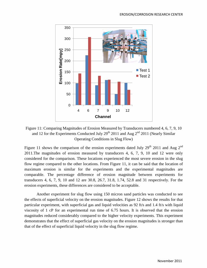
Figure 11: Comparing Magnitudes of Erosion Measured by Transducers numbered 4, 6, 7, 9, 10
and 12 for the Experiments Conducted July 29th
2011 and Aug 2nd
2011 (Nearly Similar
Operating Conditions in Slug Flow)
Figure 11 shows the comparison of the erosion experiments dated July 29th
2011 and Aug 2nd
2011.The magnitudes of erosion measured by transducers 4, 6, 7, 9, 10 and 12 were only
considered for the comparison. These locations experienced the most severe erosion in the slug
flow regime compared to the other locations. From Figure 11, it can be said that the location of
maximum erosion is similar for the experiments and the experimental magnitudes are
comparable. The percentage difference of erosion magnitude between experiments for
transducers 4, 6, 7, 9, 10 and 12 are 30.8, 26.7, 31.8, 1.74, 52.8 and 31 respectively. For the
erosion experiments, these differences are considered to be acceptable.
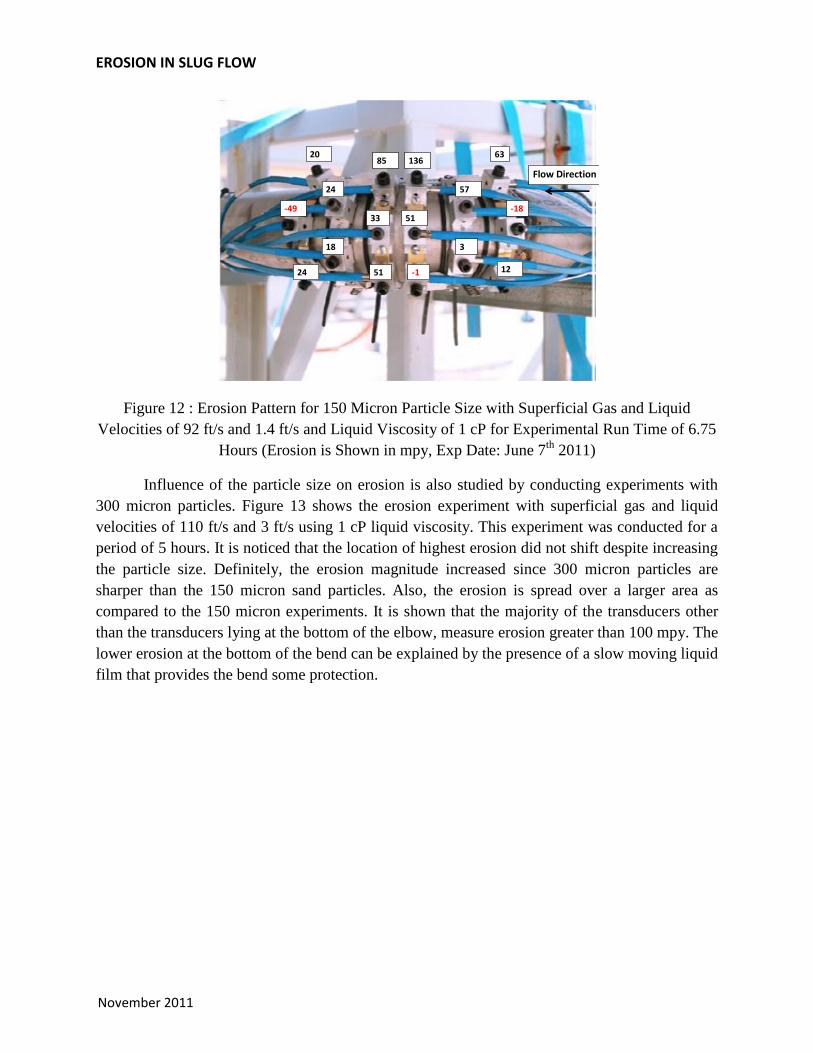
Another experiment for slug flow using 150 micron sand particles was conducted to see
the effects of superficial velocity on the erosion magnitudes. Figure 12 shows the results for that
particular experiment, with superficial gas and liquid velocities as 92 ft/s and 1.4 ft/s with liquid
viscosity of 1 cP for an experimental run time of 6.75 hours. It is observed that the erosion
magnitudes reduced considerably compared to the higher velocity experiments. This experiment
demonstrates that the effect of superficial gas velocity on the erosion magnitudes is stronger than
that of the effect of superficial liquid velocity in the slug flow regime.
0
50
100
150
200
250
300
350
4 6 7 9 10 12
Ero
sio
n R
ate
[mp
y]
Channel
Test 1
Test 2
6
Flow Direction
1
2
3
5
6
8
9
11
13
14
15
16
7
412
10
EROSION IN SLUG FLOW
November 2011
Figure 12 : Erosion Pattern for 150 Micron Particle Size with Superficial Gas and Liquid
Velocities of 92 ft/s and 1.4 ft/s and Liquid Viscosity of 1 cP for Experimental Run Time of 6.75
Hours (Erosion is Shown in mpy, Exp Date: June 7th
2011)
Influence of the particle size on erosion is also studied by conducting experiments with
300 micron particles. Figure 13 shows the erosion experiment with superficial gas and liquid
velocities of 110 ft/s and 3 ft/s using 1 cP liquid viscosity. This experiment was conducted for a
period of 5 hours. It is noticed that the location of highest erosion did not shift despite increasing
the particle size. Definitely, the erosion magnitude increased since 300 micron particles are
sharper than the 150 micron sand particles. Also, the erosion is spread over a larger area as
compared to the 150 micron experiments. It is shown that the majority of the transducers other
than the transducers lying at the bottom of the elbow, measure erosion greater than 100 mpy. The
lower erosion at the bottom of the bend can be explained by the presence of a slow moving liquid
film that provides the bend some protection.
Flow Direction
63
-18
12
57
3
136
51
-1
85
33
51
24
18
20
-49
24
EROSION/CORROSION RESEARCH CENTER
November 2011
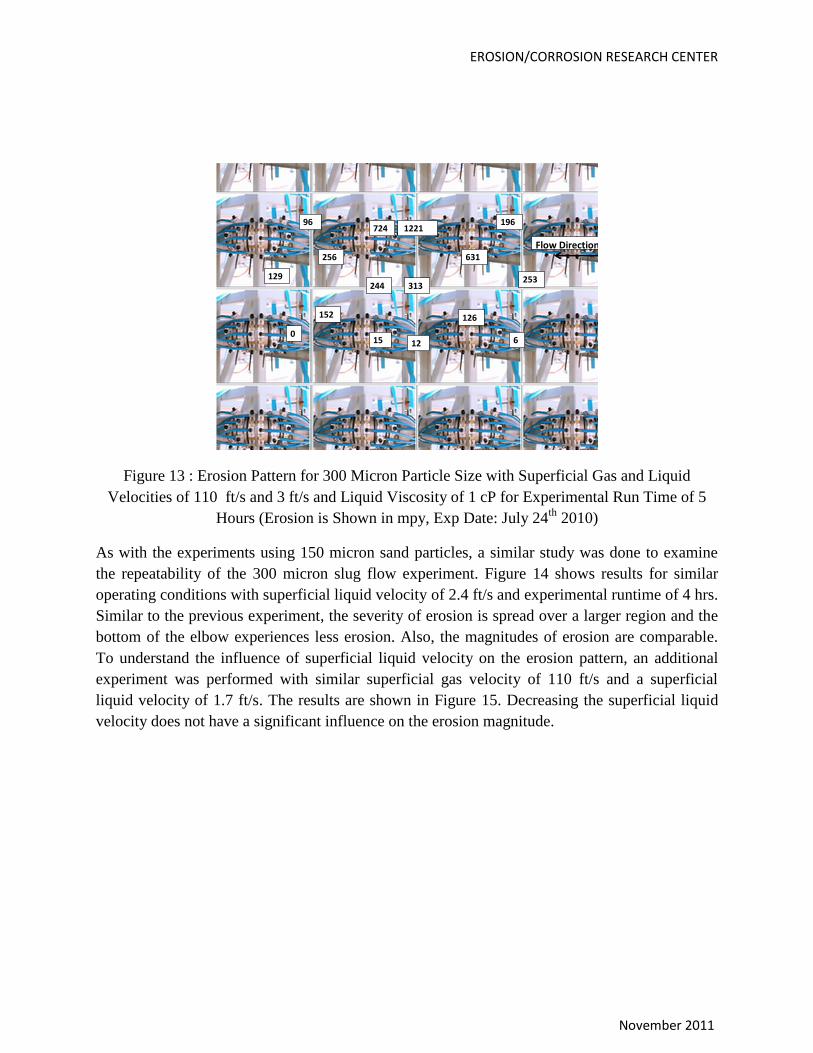
Figure 13 : Erosion Pattern for 300 Micron Particle Size with Superficial Gas and Liquid
Velocities of 110 ft/s and 3 ft/s and Liquid Viscosity of 1 cP for Experimental Run Time of 5
Hours (Erosion is Shown in mpy, Exp Date: July 24th
2010)
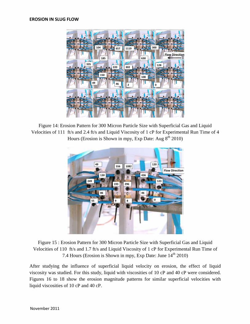
As with the experiments using 150 micron sand particles, a similar study was done to examine
the repeatability of the 300 micron slug flow experiment. Figure 14 shows results for similar
operating conditions with superficial liquid velocity of 2.4 ft/s and experimental runtime of 4 hrs.
Similar to the previous experiment, the severity of erosion is spread over a larger region and the
bottom of the elbow experiences less erosion. Also, the magnitudes of erosion are comparable.
To understand the influence of superficial liquid velocity on the erosion pattern, an additional
experiment was performed with similar superficial gas velocity of 110 ft/s and a superficial
liquid velocity of 1.7 ft/s. The results are shown in Figure 15. Decreasing the superficial liquid
velocity does not have a significant influence on the erosion magnitude.
15
196
253
6
631
126
1221
313
12
724
244
15
256
152
96
129
0
Flow Direction
EROSION IN SLUG FLOW
November 2011
Figure 14: Erosion Pattern for 300 Micron Particle Size with Superficial Gas and Liquid
Velocities of 111 ft/s and 2.4 ft/s and Liquid Viscosity of 1 cP for Experimental Run Time of 4
Hours (Erosion is Shown in mpy, Exp Date: Aug 8th
2010)
Figure 15 : Erosion Pattern for 300 Micron Particle Size with Superficial Gas and Liquid
Velocities of 110 ft/s and 1.7 ft/s and Liquid Viscosity of 1 cP for Experimental Run Time of
7.4 Hours (Erosion is Shown in mpy, Exp Date: June 14th
2010)
After studying the influence of superficial liquid velocity on erosion, the effect of liquid
viscosity was studied. For this study, liquid with viscosities of 10 cP and 40 cP were considered.
Figures 16 to 18 show the erosion magnitude patterns for similar superficial velocities with
liquid viscosities of 10 cP and 40 cP.
Flow Direction
300
128
0
630
108
1119
302
2
657
220
46
185
150
104
335
49
Flow Direction
120
123
0
436
46
1082
296
8
556
193
9
130
86
49
249
55
EROSION/CORROSION RESEARCH CENTER
November 2011
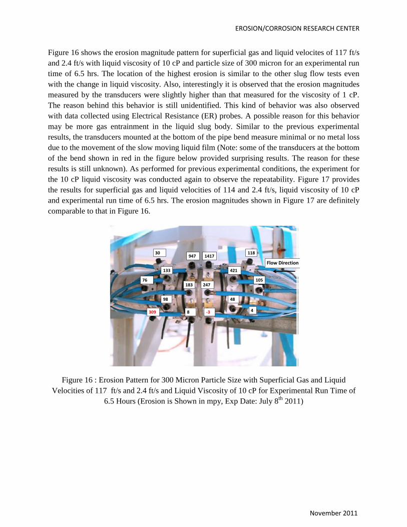
Figure 16 shows the erosion magnitude pattern for superficial gas and liquid velocites of 117 ft/s
and 2.4 ft/s with liquid viscosity of 10 cP and particle size of 300 micron for an experimental run
time of 6.5 hrs. The location of the highest erosion is similar to the other slug flow tests even
with the change in liquid viscosity. Also, interestingly it is observed that the erosion magnitudes
measured by the transducers were slightly higher than that measured for the viscosity of 1 cP.
The reason behind this behavior is still unidentified. This kind of behavior was also observed
with data collected using Electrical Resistance (ER) probes. A possible reason for this behavior
may be more gas entrainment in the liquid slug body. Similar to the previous experimental
results, the transducers mounted at the bottom of the pipe bend measure minimal or no metal loss
due to the movement of the slow moving liquid film (Note: some of the transducers at the bottom
of the bend shown in red in the figure below provided surprising results. The reason for these
results is still unknown). As performed for previous experimental conditions, the experiment for
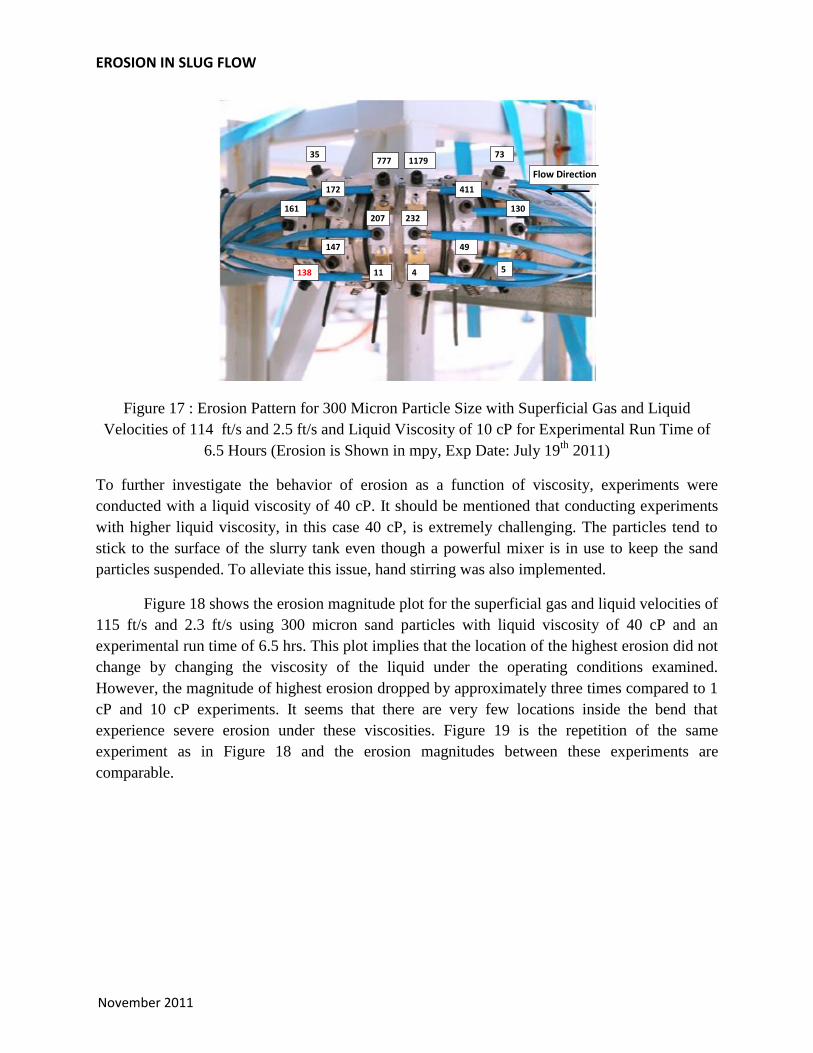
the 10 cP liquid viscosity was conducted again to observe the repeatability. Figure 17 provides
the results for superficial gas and liquid velocities of 114 and 2.4 ft/s, liquid viscosity of 10 cP
and experimental run time of 6.5 hrs. The erosion magnitudes shown in Figure 17 are definitely
comparable to that in Figure 16.
Figure 16 : Erosion Pattern for 300 Micron Particle Size with Superficial Gas and Liquid
Velocities of 117 ft/s and 2.4 ft/s and Liquid Viscosity of 10 cP for Experimental Run Time of
6.5 Hours (Erosion is Shown in mpy, Exp Date: July 8th
2011)
Flow Direction
118
105
4
421
48
1417
247
-3
947
183
8
133
98
30
76
309
EROSION IN SLUG FLOW
November 2011
Figure 17 : Erosion Pattern for 300 Micron Particle Size with Superficial Gas and Liquid
Velocities of 114 ft/s and 2.5 ft/s and Liquid Viscosity of 10 cP for Experimental Run Time of
6.5 Hours (Erosion is Shown in mpy, Exp Date: July 19th
2011)
To further investigate the behavior of erosion as a function of viscosity, experiments were
conducted with a liquid viscosity of 40 cP. It should be mentioned that conducting experiments
with higher liquid viscosity, in this case 40 cP, is extremely challenging. The particles tend to
stick to the surface of the slurry tank even though a powerful mixer is in use to keep the sand
particles suspended. To alleviate this issue, hand stirring was also implemented.
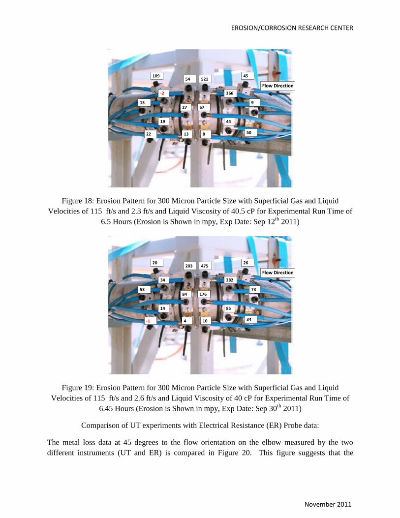
Figure 18 shows the erosion magnitude plot for the superficial gas and liquid velocities of
115 ft/s and 2.3 ft/s using 300 micron sand particles with liquid viscosity of 40 cP and an
experimental run time of 6.5 hrs. This plot implies that the location of the highest erosion did not
change by changing the viscosity of the liquid under the operating conditions examined.
However, the magnitude of highest erosion dropped by approximately three times compared to 1
cP and 10 cP experiments. It seems that there are very few locations inside the bend that
experience severe erosion under these viscosities. Figure 19 is the repetition of the same
experiment as in Figure 18 and the erosion magnitudes between these experiments are
comparable.
Flow Direction
73
130
5
411
49
1179
232
4
777
207
11
172
147
35
161
138
EROSION/CORROSION RESEARCH CENTER
November 2011
Figure 18: Erosion Pattern for 300 Micron Particle Size with Superficial Gas and Liquid
Velocities of 115 ft/s and 2.3 ft/s and Liquid Viscosity of 40.5 cP for Experimental Run Time of
6.5 Hours (Erosion is Shown in mpy, Exp Date: Sep 12th
2011)
Figure 19: Erosion Pattern for 300 Micron Particle Size with Superficial Gas and Liquid
Velocities of 115 ft/s and 2.6 ft/s and Liquid Viscosity of 40 cP for Experimental Run Time of
6.45 Hours (Erosion is Shown in mpy, Exp Date: Sep 30th
2011)
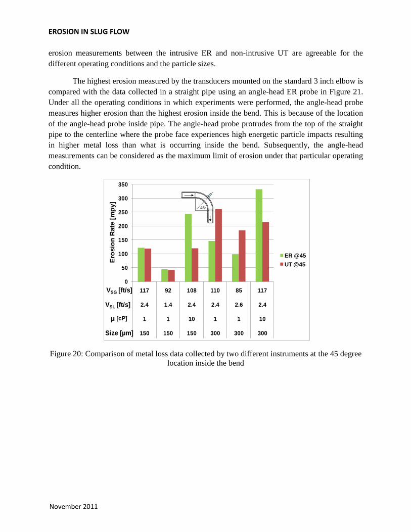
Comparison of UT experiments with Electrical Resistance (ER) Probe data:
The metal loss data at 45 degrees to the flow orientation on the elbow measured by the two
different instruments (UT and ER) is compared in Figure 20. This figure suggests that the
Flow Direction
45
9
50
266
44
521
67
8
54
27
13
-2
19
109
15
22
16
Flow Direction
26
73
34
282
85
475
176
10
203
84
4
34
14
20
53
-1
EROSION IN SLUG FLOW
November 2011
erosion measurements between the intrusive ER and non-intrusive UT are agreeable for the
different operating conditions and the particle sizes.
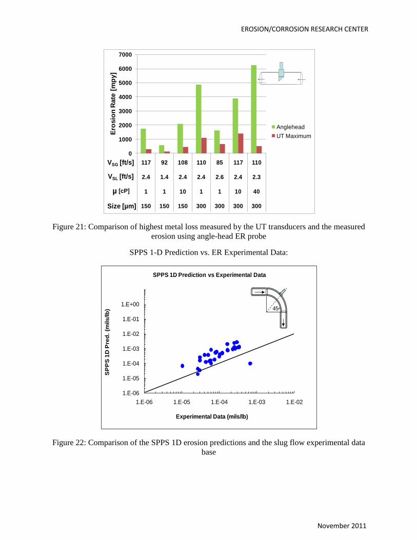
The highest erosion measured by the transducers mounted on the standard 3 inch elbow is
compared with the data collected in a straight pipe using an angle-head ER probe in Figure 21.
Under all the operating conditions in which experiments were performed, the angle-head probe
measures higher erosion than the highest erosion inside the bend. This is because of the location
of the angle-head probe inside pipe. The angle-head probe protrudes from the top of the straight
pipe to the centerline where the probe face experiences high energetic particle impacts resulting
in higher metal loss than what is occurring inside the bend. Subsequently, the angle-head
measurements can be considered as the maximum limit of erosion under that particular operating
condition.
Figure 20: Comparison of metal loss data collected by two different instruments at the 45 degree
location inside the bend
0
50
100
150
200
250
300
350
117 92 108 110 85 117
2.4 1.4 2.4 2.4 2.6 2.4
1 1 10 1 1 10
150 150 150 300 300 300
Ero
sio
n R
ate
[m
py]
ER @45
UT @45
45o
VSG [ft/s]
VSL [ft/s]
µ [cP]
Size [µm]
EROSION/CORROSION RESEARCH CENTER
November 2011
Figure 21: Comparison of highest metal loss measured by the UT transducers and the measured
erosion using angle-head ER probe
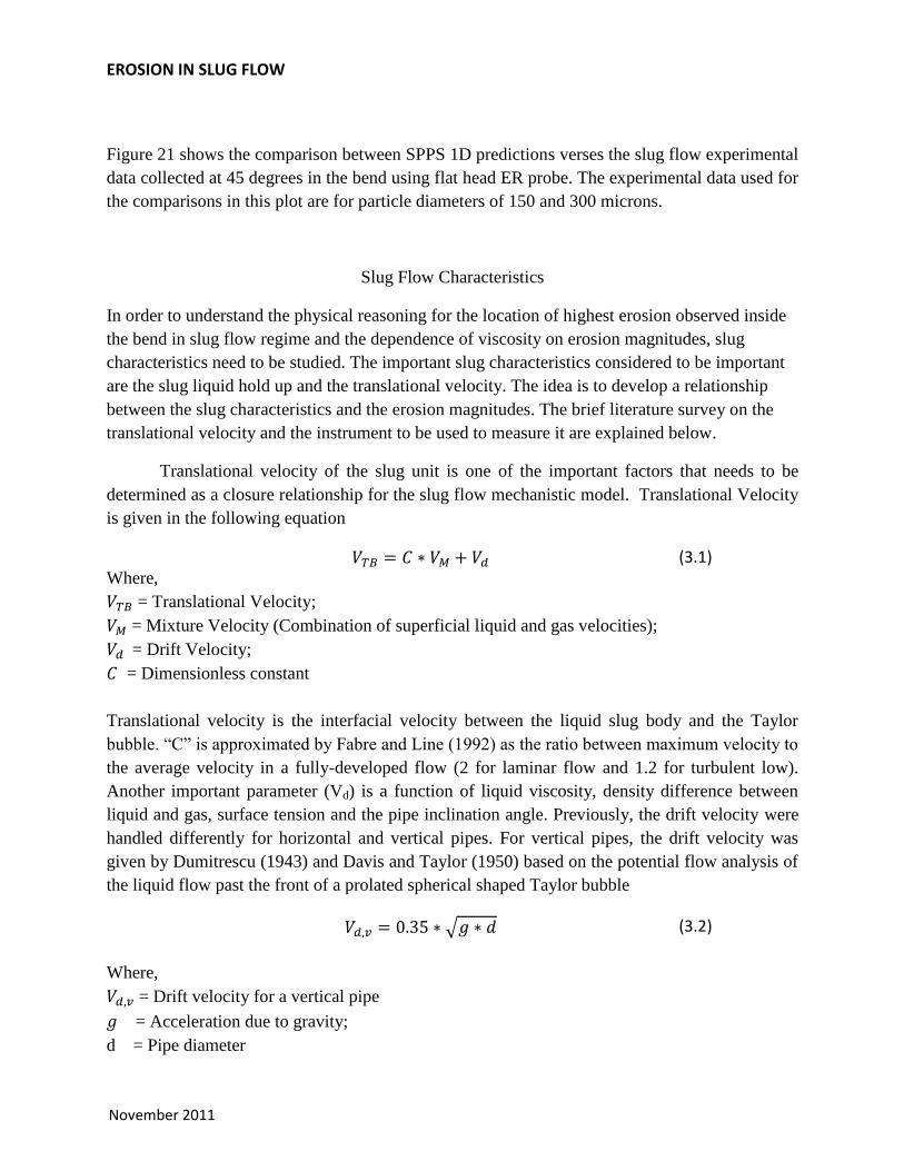
SPPS 1-D Prediction vs. ER Experimental Data:
Figure 22: Comparison of the SPPS 1D erosion predictions and the slug flow experimental data
base
0
1000
2000
3000
4000
5000
6000
7000
117 92 108 110 85 117 110
2.4 1.4 2.4 2.4 2.6 2.4 2.3
1 1 10 1 1 10 40
150 150 150 300 300 300 300
Ero
sio
n R
ate
[m
py]
Anglehead
UT Maximum
VSL [ft/s]
VSG [ft/s]
µ [cP]
Size [µm]
1.E-06
1.E-05
1.E-04
1.E-03
1.E-02
1.E-01
1.E+00
1.E-06 1.E-05 1.E-04 1.E-03 1.E-02
SP
PS
1D
Pre
d.
(mils
/lb
)
Experimental Data (mils/lb)
SPPS 1D Prediction vs Experimental Data
45o
EROSION IN SLUG FLOW
November 2011
Figure 21 shows the comparison between SPPS 1D predictions verses the slug flow experimental
data collected at 45 degrees in the bend using flat head ER probe. The experimental data used for
the comparisons in this plot are for particle diameters of 150 and 300 microns.
Slug Flow Characteristics
In order to understand the physical reasoning for the location of highest erosion observed inside
the bend in slug flow regime and the dependence of viscosity on erosion magnitudes, slug
characteristics need to be studied. The important slug characteristics considered to be important
are the slug liquid hold up and the translational velocity. The idea is to develop a relationship
between the slug characteristics and the erosion magnitudes. The brief literature survey on the
translational velocity and the instrument to be used to measure it are explained below.
Translational velocity of the slug unit is one of the important factors that needs to be
determined as a closure relationship for the slug flow mechanistic model. Translational Velocity
is given in the following equation
(3.1) Where,
= Translational Velocity;
= Mixture Velocity (Combination of superficial liquid and gas velocities);
= Drift Velocity;
= Dimensionless constant
Translational velocity is the interfacial velocity between the liquid slug body and the Taylor
bubble. “C” is approximated by Fabre and Line (1992) as the ratio between maximum velocity to
the average velocity in a fully-developed flow (2 for laminar flow and 1.2 for turbulent low).
Another important parameter (Vd) is a function of liquid viscosity, density difference between
liquid and gas, surface tension and the pipe inclination angle. Previously, the drift velocity were
handled differently for horizontal and vertical pipes. For vertical pipes, the drift velocity was
given by Dumitrescu (1943) and Davis and Taylor (1950) based on the potential flow analysis of
the liquid flow past the front of a prolated spherical shaped Taylor bubble
(3.2)
Where,
= Drift velocity for a vertical pipe
= Acceleration due to gravity;
d = Pipe diameter
EROSION/CORROSION RESEARCH CENTER
November 2011
There was controversy on the drift velocity for horizontal pipe flow. Some investigators argued
there should be zero drift velocity for the horizontal case. However, other experimental and
theoretical studies confirmed a drift velocity in the horizontal pipe and its value exceeds that in
vertical flow. The reason for the drift velocity in the horizontal pipe is due to the hydrostatic
difference of pressure between the top and bottom of the Taylor bubble nose. According to
Benjamin’s (1968) analysis, drift velocity for the horizontal flow ( ) based on inviscid
potential flow analysis is given as
(3.3)
Bendikson (1984) conducted an experimental study for the drift velocity at various inclinations
of the pipe flow. He proposed a correlation which is given below
(3.4)
The drift velocity behaves interestingly as a function of the inclination angle. It achieves a
maximum velocity around 300 and a minimum at 90
0. The reason may be due to the balance
between the gravitational potential and the film drainage. Another, possible reason is the contact
angle between the Taylor bubble and the top wall of the pipe. The contact angle is acute from
horizontal to around 300 and is obtuse afterwards. At an angle around 30
0, the contact angle is
900 allowing greater film drainage and resulting in higher drift velocity. Similarly when the pipe
is in its vertical orientation, the gravitational potential is higher and the Taylor bubble is
axisymmetric pushing the liquid film around it in the radial direction making it thinner, there is
less film drainage and in turn lower drift velocity.
Thus, the interface velocity of the liquid slug and the Taylor bubble is given below
(3.5)
The instrument for the measurement of slug characteristics to be used in the future is explained
below:
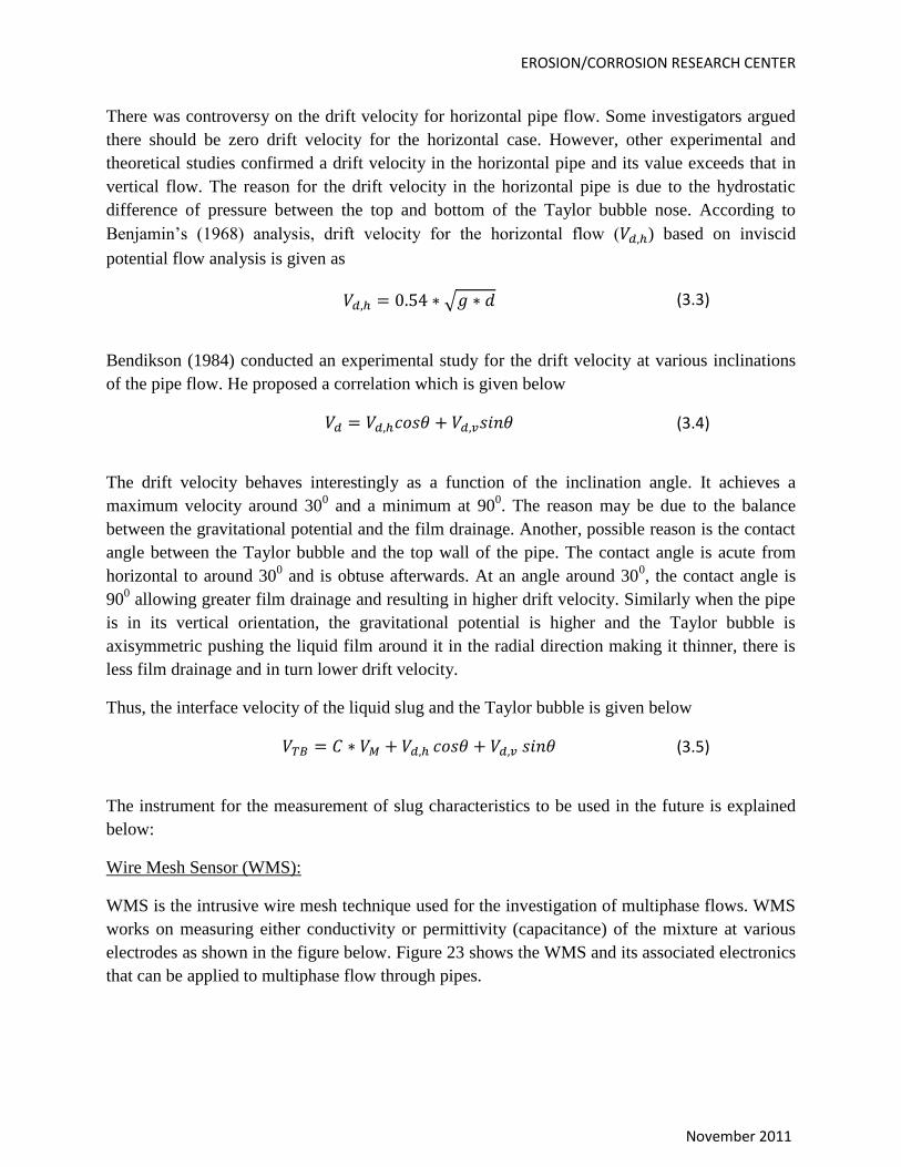
Wire Mesh Sensor (WMS):
WMS is the intrusive wire mesh technique used for the investigation of multiphase flows. WMS
works on measuring either conductivity or permittivity (capacitance) of the mixture at various
electrodes as shown in the figure below. Figure 23 shows the WMS and its associated electronics
that can be applied to multiphase flow through pipes.
EROSION IN SLUG FLOW
November 2011
Figure 23: Capacitance Wire Mesh Sensor (Courtesy: HZDR, Dresden, Germany)
WMS can measure average liquid hold-up in the liquid slug and the entrainment fraction of
liquid in the Taylor bubble region for pseudo slug flow and also the interface velocity. This
information is useful to improve our current slug flow erosion model by the understanding
enhanced by developing a relationship between slug characteristics and the erosion magnitudes.
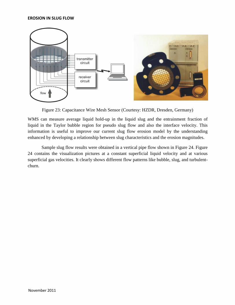
Sample slug flow results were obtained in a vertical pipe flow shown in Figure 24. Figure
24 contains the visualization pictures at a constant superficial liquid velocity and at various
superficial gas velocities. It clearly shows different flow patterns like bubble, slug, and turbulent-
churn.
EROSION/CORROSION RESEARCH CENTER
November 2011
Figure 24: 3-D Visualization Obtained from WMS at a Constant Liquid Superficial Velocity (1
m/s) and at different Superficial Gas Velocities (Transient Two Phase Flow Test Facility,
Germany)
Conclusions
The conclusions from the current study are shown below:
1. Erosion pattern in a standard 3-inch elbow is shown
2. Location of higher erosion is identified
3. In horizontal slug flow, the metal loss is higher on the top of the elbow and lower at the
bottom.
4. There is a slight increase in erosion magnitude in a bend for 10 cP viscous liquid
compared to 1 cP. However, there is a radical decrease in the erosion magnitude after
increasing the liquid viscosity to 40 cP.
5. Metal loss measured in straight pipe using angle-head probe is always higher than the
highest erosion inside the bend for the conditions examined
Future Work
In order to better understand the erosion mechanism, following work will be conducted in the
future.
EROSION IN SLUG FLOW
November 2011
1. Use WMS and high speed photography in plug, slug and pseudo-slug regimes to measure
a. Slug Length
b. Translational (Interface) Velocity
c. Slug Frequency
d. Slug Liquid Hold-Up
2. Develop a relationship between slug characteristics and the erosion magnitude
3. Perform sand sampling experiments in a horizontal pipe and in the bend
4. Improve the slug flow SPPS model with the understanding obtained through experiments