Equivariant Gromov-Witten Theory ofGKM Orbifolds

Zhengyu Zong

Submitted in partial fulfillment of therequirements for the degree

of Doctor of Philosophyin the Graduate School of Arts and Sciences

COLUMBIA UNIVERSITY

2015

©2014Zhengyu Zong

All Rights Reserved

ABSTRACT

Equivariant Gromov-Witten Theory ofGKM Orbifolds

Zhengyu Zong

In this paper, we study the all genus Gromov-Witten theory for any

GKM orbifold X. We generalize the Givental formula which is studied in

the smooth case in [41] [42] [43] to the orbifold case. Specifically, we recover

the higher genus Gromov-Witten invariants of a GKM orbifold X by its

genus zero data. When X is toric, the genus zero Gromov-Witten invariants

of X can be explicitly computed by the mirror theorem studied in [22] and

our main theorem gives a closed formula for the all genus Gromov-Witten

invariants of X. When X is a toric Calabi-Yau 3-orbifold, our formula leads

to a proof of the remodeling conjecture in [38]. The remodeling conjecture

can be viewed as an all genus mirror symmetry for toric Calabi-Yau 3-

orbifolds. In this case, we apply our formula to the A-model higher genus

potential and prove the remodeling conjecture by matching it to the B-model

higher genus potential.

Table of Contents

1 Introduction 11.1 background and motivation . . . . . . . . . . . . . . . . . . . . . 11.2 Plan of the paper . . . . . . . . . . . . . . . . . . . . . . . . . . . 4

2 Equivariant Chen-Ruan cohomology of GKM orbifolds 72.1 GKM orbifolds . . . . . . . . . . . . . . . . . . . . . . . . . . . . 82.2 Chen-Ruan orbifold cohomology . . . . . . . . . . . . . . . . . . 10

2.2.1 The inertia stack . . . . . . . . . . . . . . . . . . . . . . 102.2.2 Chen-Ruan orbifold cohomology . . . . . . . . . . . . . 12

2.3 Equivariant Chen-Ruan cohomology of GKM orbifolds . . . . 142.3.1 The simplest case: X = [Cr/G] . . . . . . . . . . . . . . 142.3.2 The general case . . . . . . . . . . . . . . . . . . . . . . . 17

3 Gromov-Witten theory, quantum cohomology and Frobe-nius manifolds 193.1 Gromov-Witten theory of smooth Deligne-Mumford stacks . . 203.2 Gromov-Witten theory of GKM orbifolds . . . . . . . . . . . . 213.3 Frobenius manifolds and semisimplicity . . . . . . . . . . . . . 233.4 Solutions to the quantum differential equations . . . . . . . . . 25

4 Higher genus Gromov-Witten potential 274.1 quantization of quadratic Hamiltonians . . . . . . . . . . . . . 27

4.1.1 Symplectic space formalism . . . . . . . . . . . . . . . . 274.1.2 Quantization of quadratic Hamiltonians . . . . . . . . . 29

4.2 Higher genus structure . . . . . . . . . . . . . . . . . . . . . . . 304.2.1 The quantization procedure and group actions on co-

homological field theories . . . . . . . . . . . . . . . . . 314.2.2 The graph sum formula . . . . . . . . . . . . . . . . . . 35

4.3 Reconstruction from genus zero data . . . . . . . . . . . . . . . 40

i

4.3.1 The case X = [Cr/G] and orbifold quantum Riemann-Roch theorem . . . . . . . . . . . . . . . . . . . . . . . . 40

4.3.2 The general case . . . . . . . . . . . . . . . . . . . . . . . 43

5 Application: all genus mirror symmetry for toric Calabi-Yau3-orbifolds 465.1 Introduction . . . . . . . . . . . . . . . . . . . . . . . . . . . . . . 465.2 A-model geometry . . . . . . . . . . . . . . . . . . . . . . . . . . 50

5.2.1 Toric Calabi-Yau 3-orbifolds . . . . . . . . . . . . . . . . 505.2.2 A-model topological string . . . . . . . . . . . . . . . . . 51

5.3 B-model geometry . . . . . . . . . . . . . . . . . . . . . . . . . . 555.3.1 Mirror curve and dimensional reduction of the Landau-

Ginzburg model . . . . . . . . . . . . . . . . . . . . . . . 555.3.2 The Liouville form . . . . . . . . . . . . . . . . . . . . . 575.3.3 Lefshetz thimbles . . . . . . . . . . . . . . . . . . . . . . 585.3.4 Differentials of the second kind . . . . . . . . . . . . . . 585.3.5 Oscillating integrals and the B-model S-matrix . . . . 605.3.6 The f -matrix and the B-model R-matrix . . . . . . . . 615.3.7 The Eynard-Orantin topological recursion and the B-

model graph sum . . . . . . . . . . . . . . . . . . . . . . 615.4 The remodeling conjecture: all genus open-closed mirror sym-

metry . . . . . . . . . . . . . . . . . . . . . . . . . . . . . . . . . . 635.4.1 Identification of fundamental solutions of A-model and

B-model quantum differential equations . . . . . . . . . 635.4.2 Identification of graph sums . . . . . . . . . . . . . . . . 645.4.3 Generalization to the multi-branes case . . . . . . . . . 69

Bibliography . . . . . . . . . . . . . . . . . . . . . . . . . . . . . . . . . 71

ii

ACKNOWLEDGEMENTS

First of all, I wish to express my deepest thanks to my advisor Chiu-Chu

Melissa Liu. From the start of my time in graduate school, she led me to

this fascinating area by introducing reading materials to me. She chose each

article and text book carefully which made me get into this area quickly.

Then she proposed wonderful problems for me to study. In this process,

she provided me invaluable guidance and advice and constantly encouraged

me. Whenever I met difficulties in my research, she always made herself

extremely available to me. She has always been patient to discuss various

questions with me no matter these questions were easy or difficult. She

showed me details of various computation processes, helped me to learn

basic skills by providing me her own notes, taught me latex skills by hand

and explained so many fundamental concepts to me. On the other hand, her

wisdom and insight in mathematics guided me through the whole process

of my research and pointed the right direction of my work. It has been

always exciting to work with her. She made me realize that one can work

out beautiful results with deep interest in mathematics. I always learned a

lot from discussions with her and I look forward to continuing to learn from

her in the future.

I also wish to thank Bohan Fang. It has been a joy to work with him

iii

and Melissa on various topics in mirror symmetry. I learned a lot from

him, especially in the areas of homological mirror symmetry and B-model

geometry. I also wish to thank Dustin Ross. I learned a lot from him

when we worked on the topics in Gromov-Witten/Donaldson-Thomas cor-

respondence for orbifolds. Many thanks to Davesh Maulik, Yongbin Ruan,

Renzo Cavalieri, Jun Li, Jim Bryan, Ravi Vakil, Motohico Mulase, Yu-Shen

Lin, Yefeng Shen, Nicolas Orantin, Bertrand Eynard, Vincent Bouchard,

Jian Zhou, Hsian-Hua Tseng and Artan Sheshmani for their useful com-

munications. Thanks to my classmates with whom I enjoyed my study of

mathematics. Special thanks to Terrance Cope who helped me in so many

aspects during my Ph.D study.

Finally, I wish to thank my parents who make me live a happy life.

Particular thanks to my mother who loves me so much. She gives me the

braveness to discover the truths in the world and overcome the difficulties

on my way. She gives me the heart to seek happiness and bring happiness to

people in the world. She gives me the soul to feel the brightness and bring

the brightness to the world.

iv

Chapter 1

Introduction

1.1 background and motivation

Let X be an algebraic GKM manifold, which means that there exists an

algebraic torus T acting on X such that there are only finitely many fixed

points and finitely many 1-dimensional orbit. In the sequence of papers [41]

[42] [43], Givental studies the all genus equivariant Gromov-Witten theory of

a GKM manifold X. He obtains a formula for the full descendent potential of

X and conjectures that the same formula is true for any X with semisimple

Frobenius manifold. This formula is often referred to Givental formula. It

expresses the higher genus Gromov-Witten invariants of X in terms of the

genus 0 data. The key point is that the genus 0 data in that formula can

1

be expressed in abstract terms of semisimple Frobenius structures and vice

versa. So one can reconstruct the higher genus Gromov-Witten theory of X

by its Frobenius structure.

When X is toric, one can build the mirror symmetry between X and

its Landau-Ginzburg mirror. The mirror theorem [40], [57, 58, 59, 60] for

smooth toric varieties gives an isomorphism between the quantum coho-

mology ring of X and the Jacobi ring of its Landau-Ginzburg mirror. So

one can identify the Frobenius structures of these two rings. In particu-

lar, the quantum differential equations in A and B-model can be identified.

Under this identification, the genus 0 data in Givental formula can be de-

scribed explicitly on B-model side. For example, the data coming from the

fundamental solution of the quantum differential equation can be give by

oscillatory integrals over the Lefschetz thimbles on B-model side, the norm-

s of the canonical basis is related to the Hessians at the critical points of

the super potential and so on. Of course, the above procedure can also be

generalized to other homogeneous spaces such as Grassmannians.

It is natural to ask whether the Givental formula can be generalized to

the orbifold case. On the Gromov-Witten theory side, one wants to study the

higher genus equivariant orbifold Gromov-Witten theory for GKM orbifolds

such as toric orbifolds and other homogeneous orbifold spaces. So we want

to obtain an orbifold Givental formula so that we can recover the higher

genus data by the Frobenius structures of the target X. When X is toric,

the orbifold mirror theorem is proved in [22]. Just as the smooth case, one

2

can identify the quantum cohomology ring of X to the Jacobi ring of its

mirror. So we can give nice explicit explanations of the Frobenius structure

of X in terms of corresponding structures in B-model. Therefore if we can

obtain an orbifold version of the Givental formula, the higher genus Gromov-

Witten theory of X can be recovered effectively by concrete data. This idea

also applies to many other GIT quotients where similar mirror symmetry

phenomenon arises [19].

Perhaps, the most interesting case is when X is a toric Calabi-Yau 3-

orbifold. In this case, the remodeling conjecture is established in [65] [8] and

[9]. The remodeling conjecture gives us a higher genus B-model which it-

self arises naturally in the matrix-model theory. The remodeling conjecture

claims that the B-model higher genus potential can be identified with the

A-model higher genus potential, which can be viewed as a all genus mir-

ror symmetry statement. The higher genus B-model potential is obtained

by applying the Eynard-Orantin recursion to the mirror curve of X. This

potential has a graph sum formula which has exactly the same form of the

corresponding graph sum of Givental formula on A-model side . The identi-

fication of the higher genus potentials is then reduced to the identification of

Frobenius structures which can be deduced from the genus 0 mirror theorem

[22]. So the proof of the orbifold Givental formula plays a crucial role in

proving the remodeling conjecture (see [38]). Besides, one needs to study

the Frobenius structures that appear in the Givental formula carefully in

order to match them to the corresponding structures on the B-model side.

3

To prove the remodeling conjecture [38] is one of the main reasons for the

author to study the orbifold Givental formula.

For higher dimensional toric orbifolds, one can try to generalize the

Eynard-Orantin recursion to higher dimensional varieties. This may gen-

eralize the remodeling conjecture to higher dimensional toric orbifolds. This

may be a further application of the orbifold Givental formula.

1.2 Plan of the paper

In Chapter 2, we first study the geometry of an GKM orbifold X. Then

we review the definition of the Chen-Ruan orbifold cohomology of smooth

Deligne-Mumford stacks. After that we move on to the equivariant Chen-

Ruan cohomology of an GKM orbifold X. It turns out that the equivariant

Chen-Ruan cohomology ring is a semisimple Frobenius algebra.

In Chapter 3, we first review several definitions about the orbifold Gromov-

Witten theory of smooth Deligne-Mumford stacks. Then we apply these def-

initions to the equivariant Gromov-Witten theory of an GKM orbifold X.

Then we will deduce the semisimplicity of the Frobenius manifold of X from

the semisimplicity of its classical equivariant Chen-Ruan cohomology. After

that we will consider the quantum differential equation and its fundamental

solutions. One of them is given explicitly by the 1-primary 1-descendent

genus 0 potential. This solution will play a special role in the later.

In Chapter 4, we move on to the higher genus structures. We will first

4

review the quantization procedure which will be used in the later sections.

The we obtain the orbifold Givental formula by applying Teleman’s result

[66] of classification of 2D semisimple field theories to our case. Since the

Frobenius manifold of X is semisimple, the cohomological field theory of X

coming from the Gromov-Witten theory lies in the same orbit of the trivial

field theory of the same Frobenius manifold under certain group actions. The

Givental formula can be derived using this group action point of view. Then

we give a more explicit graph sum formula for the higher genus potential

of X. This graph sum formula is crucial in the proof of the remodeling

conjecture [38]. We will discuss the remodeling conjecture in Chapter 5.

We also need to fix the ambiguity of the R−operator in Givental formula.

Since we are working with equivariant Gromov-Witten theory, our Frobenius

structure is not conformal. Therefore the ambiguity with the R−operator

in Givental formula cannot be fixed by the usual method using the Euler

vector field. Instead, we use the structure of solution space to the quantum

differential equation (Theorem 5.1). Then we know that the ambiguity is

a constant matrix. So we study the case when the degree is 0 and when

there is no primary insertion and compare the Givental formula in this case

with the orbifold quantum Riemann-Roch theorem in [67]. In the end, we

obtain the reconstruction theorem by expressing the R−operator in terms of

the quantum multiplication law and the explicit constant matrix given by

orbifold quantum Riemann-Roch theorem.

In Chapter 5, we apply the Givental quantization formula to the case

5

when X is a toric Calabi-Yau 3-orbifold. In this case, one can consider

the remodeling conjecture which is an all genus mirror symmetry for toric

Calabi-Yau 3-orbifolds. In this conjecture, the A-model higher genus poten-

tial is the open Gromov-Witten potential of X with respect to one or several

Aganagic-Vafa branes on X. The higher genus B-model ωg,n is obtained by

applying the Eynard-Orantin [32] topological recursion to the mirror curve

C of X. It is a symmetric n-form on C. When ωg,n is expanded around

certain points on C, the coefficients will give us the open Gromov-Witten

invariants of X. On the other hand, we also have the Landau-Ginzburg

mirror of X, which contains a super potential W T ∶ (C∗)3 → C. The mirror

curve is related to the Landau-Ginzburg mirror by the dimensional reduc-

tion. By the genus 0 mirror theorem [22], the quantum cohomology ring of

X is isomorphic to the Jacobi ring of W T . Therefore we can identify the

Frobenius structure of X with the genus 0 data coming from the Eynard-

Orantin topological recursion on the mirror curve. The bridge relating the

A-model and B-model higher genus potentials is the graph sum formula,

which is equivalent to both the quantization formula and the recursive for-

mula. From this point of view, the remodeling conjecture is proved by re-

alizing both A-model and B-model higher genus potentials as quantizations

on two isomorphic semi-simple Frobenius manifolds.

6

Chapter 2

Equivariant Chen-Ruan

cohomology of GKM

orbifolds

In this chapter, we discuss the geometry and basic properties of any GKM

orbifold X. We will study the classical equivariant Chen-Ruan cohomology

ring of X and construct its canonical basis.

The concept of a GKM manifold is first established in [44] by Goresky-

Kottwitz-MacPherson. An algebraic GKM manifold is a smooth algebraic

variety with an algebraic action of a torus T = (C∗)m, such that there are

finitely many torus fixed points and finitely many one-dimensional orbits.

Examples of algebraic GKM manifolds include toric manifolds, Grassmani-

ans, flag manifolds and so on. The advantage of a GKM manifold X is that

7

one can study the classical equivariant cohomology of X and the Atiyah-Bott

localization via the combinatorics tool called GKM graphs. This might be

the original motivation for people to study GKM manifolds. By generaliz-

ing the classical Atiyah-Bott localization to the virtual localization, one can

compute the equivariant Gromov-Witten invariants of an algebraic GKM

manifold in terms of summing over GKM graphs (see [63] for more details).

The localization procedure in this case is completely similar to that in the

toric case.

In this chapter, we study the classical equivariant Chen-Ruan cohomolo-

gy of any GKM orbifold X, which is a generalization of the GKM manifold.

The discussion of equivariant Gromov-Witten theory of X is in the next

chapter.

2.1 GKM orbifolds

Let X be an r−dimensional smooth proper Deligne-Mumford stack with a

quasi-projective coarse moduli space. Let T = (C∗)m be an algebraic torus

acting on X.

Definition 2.1.1. We say that X is a GKM orbifold if

1. There are finitely many T−fixed points.

2. There are finitely many one-dimensional orbits.

In our definition, X can be noncompact and can have nontrivial generic

stabilizers.

8

Let p1,⋯, pn be the T−fixed points of X. These points may be stacky and

locally around each pσ, the tangent space TpσX is isomorphic to [Cr/Gσ]

with Gσ a finite group and with the r axes the corresponding r one dimen-

sional orbits containing pσ, σ = 1,⋯, n. The action of Gσ on the tangent

space TpσX is a representation ρσ ∶ Gσ → GL(r,C). Since T acts on X,

we know that the action of T commutes with the action of Gσ. So the

image of the representation ρσ ∶ Gσ → GL(r,C) must be contained in the

maximal torus (note that there are only finitely many one-dimensional or-

bits and hence the T−characters along any two axes of [Cr/Gσ] are linearly

independent). Therefore, ρσ splits into r one-dimensional representations

χσj ∶ Gσ → C∗, j = 1,⋯, r. Let µlσj = χσj(Gσ) = z ∈ C∗∣zlσj = 1 ⊆ C∗,

σ = 1,⋯, n, j = 1,⋯, r.

Let N = Hom(C∗, T ) be the lattice of 1-parameter subgroups of T and

M = Hom(T,C∗) the lattice of irreducible characters of T . Then M is the

dual lattice of N and we have a canonical identification M ≅ H2T (pt,Z).

Here H∗T (pt,Z) denotes the T -equivariant cohomology of a point. Let wσj

be the character of the T−action along the j−th tangent direction at pi.

Then wσj lies in H2T (pt,Q) ≅MQ ∶=M ⊗Z Q. The rational coefficient here

is used to adapt the orbifold structure at pσ.

9

2.2 Chen-Ruan orbifold cohomology

In this section, we review the definition and basic properties of the Chen-

Ruan orbifold cohomology [18] of a smooth Deligne-Mumford stack X.

2.2.1 The inertia stack

Definition 2.2.1. Let X be a Deligne-Mumford stack. The inertia stack

IX associated to X is defined to be the fiber product

IX =X ×∆,X×X,∆ X,

where ∆ ∶X →X ×X is the diagonal morphism.

The objects in the category IX can be described as

Ob(IX) = (x, g)∣x ∈ Ob(X), g ∈ AutX(x).

The morphisms between two objects in the category IX are

HomIX((x1, g1), (x2, g2)) = h ∈ HomX(x1, x2)∣hg1 = g2h.

In particular,

AutIX(x, g) = h ∈ AutX(x)∣hg = gh.

There is a natural projection q ∶ IX → X which, on objects level, sends

(x, g) to x. There is also an involution map ι ∶ IX → IX which sends (x, g)

10

to (x, g−1). The inertial stack IX is in general not connected even if X is

connected. Suppose X is connected and let

IX =⊔i∈I

Xi

be the disjoint union of connected components. There is a distinguished

component

X0 = (x, idx)∣x ∈ Ob(X)

which is isomorphic to X. The restriction of the involution map ι to Xi

gives an isomorphism between Xi and another connected component of IX.

In particular, the restriction of ι to X0 gives an identity map.

Example 2.2.2. Let G be a finite group. Consider the quotient stack BG ∶=

[pt/G] which is called the classifying space of G. There is only one object x

in BG and Hom(x,x) = G. By definition, the objects of IBG are

Ob(IBG) = (x, g)∣g ∈ G.

The morphisms between two objects (x1, g1), (x2, g2) are

Hom((x1, g1), (x2, g2)) = g ∈ G∣gg1 = g2g = g ∈ G∣g1 = g−1g2g.

So we have

IBG ≅ [G/G]

11

where G acts on G by conjugation. Therefore

IBG = ⊔(h)∈Conj(G)

(BG)(h) = ⊔(h)∈Conj(G)

[pt/C(h)]

where (h) is the conjugacy class of h ∈ G and C(h) is the centralizer of h in

G.

2.2.2 Chen-Ruan orbifold cohomology

As vector spaces, the Chen-Ruan orbifold cohomology [18] of a smooth

Deligne-Mumford stack X is the same as the usual cohomology of the inertia

stack IX. The difference is the definition of the degree. Let us first discuss

the definition of age which determines the degree of the Chen-Ruan orbifold

cohomology.

Given an object (x, g) ∈ Ob(IX), we have a linear map g ∶ TxX → TxX

such that gl = id, where l is the order of g. Let ζ = e2πi/l and then the

eigenvalues of g are given by ζc1 ,⋯, ζcr , where ci ∈ 0,⋯, l − 1, r = dimX.

Define

age(x, g) = c1 +⋯ + crl

.

The function age ∶ IX → Q is constant on each connected component Xi of

IX and we define age(Xi) to be age(x, g) for any object (x, g) in Xi.

Definition 2.2.3. Let X be a smooth Deligne-Mumford stack. The Chen-

12

Ruan orbifold cohomology group of X is defined to be

H∗CR(X) ∶=⊕

a∈QHa

CR(X)

where

HaCR(X) =⊕

i∈I

Ha−2age(Xi)(Xi).

If X is proper, the orbifold Poincare pairing is defined to be

⟨α,β⟩X =

⎧⎪⎪⎪⎪⎪⎨⎪⎪⎪⎪⎪⎩

∫Xi α ∪ ι∗i (β), Xj = ι(Xi),

0, otherwise,

where α ∈H∗(Xi) and β ∈H∗(Xj).

The product structure for the Chen-Ruan orbifold cohomology is more

subtle.

Definition 2.2.4. For any α,β ∈H∗CR(X), their orbifold product α ⋆X β is

defined as follows: For any γ ∈H∗CR(X),

⟨α ⋆X β, γ⟩X ∶= ⟨α,β, γ⟩X0,3,0,

where the right hand side will be defined in Section 3.1.

13

2.3 Equivariant Chen-Ruan cohomology of GKM

orbifolds

In this section, we focus ourselves to the case when X is a GKM orbifold. We

will show that the equivariant Chen-Ruan cohomology of X is semisimple

by constructing its canonical basis explicitly.

2.3.1 The simplest case: X = [Cr/G]

Let Conj(G) denote the set of conjugacy classes in G. Then the inertia stack

IX can be described as

IX = ⊔(h)∈Conj(G)

[(Cr)h/C(h)] = ⊔(h)∈Conj(G)

X(h)

where (h) is the conjugacy class of h ∈ G and C(h) is the centralizer of h in

G.

For any i ∈ 1,⋯, r and any h ∈ G, define ci(h) ∈ [0,1) and age(h) by

e2π√−1ci(h) = χi(h), (2.1)

age(h) =r

∑j=1

cj(h). (2.2)

As a graded vector space over C, the Chen-Ruan cohomology H∗CR(X;C)

14

of X can be decomposed as

H∗CR(X;C) = ⊕

(h)∈Conj(G)

H∗(X(h);C)[2age(h)] = ⊕(h)∈Conj(G)

C1(h),

where deg(1(h)) = 2age(h) which is independent of the choice of h in its

conjugacy class.

Let R = H∗(BT ;C) = C[u1,⋯,um], where u1,⋯,um are the first Chern

classes of the universal line bundles over BT . The T -equivariant Chen-Ruan

orbifold cohomology H∗CR,T (X;C) = ⊕(h)∈Conj(G)H

∗T (X(h);C)[2age(h)] is

an R-module. Given h ∈ G, define

eh ∶=r

∏i=1

wδci(h),0i ∈R.

Here, wi is the character of the T−action along the i−th direction. In par-

ticular,

e1 =r

∏i=1

wi.

Then the T -equivariant Euler class of 0(h) ∶= [0/C(h)] inX(h) = [(Cr)h/C(h)]

is

eT (T0(h)X(h)) = eh1(h) ∈H∗

CR,T (X(h);C) =R1(h).

Let χ1,⋯, χr ∶ G → C∗ and l1,⋯, lr ∈ Z be defined as in the previous

section. Define

R′ = C[u1,⋯,um,w1

2l11 ,⋯,w

12lrr ]

15

which is a finite extension of R. Let Q and Q′ be the fractional fields of R,

R′, respectively. We will consider the T−equivariant Chen-Ruan cohomolo-

gy ring H∗CR,T (X;Q′).

The T−equivariant Poincare pairing of H∗CR,T (X;Q′) is given by

⟨1(h),1(h′)⟩X = 1

∣C(h)∣ ⋅δ(h−1),(h′)

eh∈ Q′.

The T -equivariant orbifold cup product of H∗CR,T (X;Q′) is given by

1(h) ⋆X 1(h′) = ∑f1∈(h1),f2∈(h2)

∣C(f1f2)∣∣G∣ (

r

∏i=1

wci(h)+ci(h

′)−ci(ff′)

i )1(ff ′).

Define

1(h) ∶=1(h)

∏ri=1 wci(h)i

∈H∗CR,T (X;Q′). (2.3)

Then

⟨1(h), 1(h′)⟩X = 1

∣C(h)∣ ⋅δ(h−1),(h′)

∏ri=1 wi∈ Q′

and

1(h) ⋆X 1(h′) = ∑f1∈(h1),f2∈(h2)

∣C(f1f2)∣∣G∣ 1(ff ′).

We now define a canonical basis for the semisimple algebraH∗CR,T (X;Q′).

Let Vα∣Conj(G)∣

α=1 be the set of irreducible representations of G and let χα be

the character of Vα. For any α, define

φα =dimVα

∣G∣ ∑(h)∈Conj(G)

χα(h−1)1(h).

16

Let να = (dimVα∣G∣

)2, α = 1,⋯, ∣Conj(G)∣. Then we have

⟨φα, φα′⟩X = δα,α′να

∏ri=1 wi

and

φα ⋆X φα′ = δα,α′ φα.

Therefore, φα∣Conj(G)∣

α=1 is a canonical basis of the semisimple algebraH∗CR,T (X;Q′).

2.3.2 The general case

In general, we apply the above construction to the local geometry around

each fixed point pσ to get a set of cohomology classes φσα∣Conj(Gσ)∣α=1 , σ =

1,⋯, n. It is easy to show that

⟨φσα, φσ′α′⟩X = δσ,σ′δα,α′νσα

∏rj=1 wσj

and

φσα ⋆X φσ′α′ = δσ,σ′δα,α′ φσα.

Therefore, the algebraH∗CR,T (X;Q′) is still semisimple and φσα∣σ = 1,⋯, n,α =

1,⋯, ∣Conj(Gσ)∣ is a canonical basis of H∗CR,T (X;Q′).

Sometimes, we also consider the normalized canonical basis φσα∣σ =

1,⋯, n,α = 1,⋯, ∣Conj(Gσ)∣, where φσα is defined to be

φσα =

¿ÁÁÀ∏rj=1 wσj

νσαφσα.

17

With this definition, we have

⟨φσα, φσ′α′⟩X = δσ,σ′δα,α′

i.e. φσα has unit length.

18

Chapter 3

Gromov-Witten theory,

quantum cohomology and

Frobenius manifolds

In this chapter, we first recall some basic definitions of Gromov-Witten

theory of a smooth Deligne-Mumford stack X. The foundation of Gromov-

Witten theory of smooth Deligne-Mumford stacks is developed in [3]. The

symplectic counterpart is developed in [17]. After that, we specialized our-

selves to the equivariant Gromov-Witten theory of a GKM orbifold X. Then

we will focus on the genus zero case which determines the Frobenius struc-

ture on H∗CR,T (X;Q′) ⊗C N(X) with N(X) the Novikov ring. In partic-

ular, it gives us the structure of the quantum cohomology ring of X and

hence determines the quantum differential equation. We will discuss the

19

semisimplicity of the Frobenius structure and the solutions to the quantum

differential equation.

3.1 Gromov-Witten theory of smooth Deligne-Mumford

stacks

Let X be a smooth Deligne-Mumford stack. Let E ⊆ H2(X,Z) be the

semigroup of effective curve classes. Define the Novikov ring N(X) to be

the completion of C[E]:

N(X) = C[E] = ∑β∈E

cβQβ ∣cβ ∈ C.

Denote byMg,k(X,β) the moduli space of degree β stable maps to X from

genus g curves with k marked points. The difference from the smooth case

is that the marked points and nodes of the domain curve are allowed to

have orbifold structures with finite cyclic isotropy groups. There are k

orbifold line bundles L1,⋯,Lk on Mg,k(X,β). The fiber of Li at a point

[f ∶ (C,x1,⋯, xk)→X] ∈Mg,k(X,β) is the cotangent space at xi. Let X ′ be

the coarse moduli space of X and letMg,k(X ′, β) be the usual moduli space

of stable maps to X ′. We still have the corresponding line bundles L′1,⋯,L′k

onMg,k(X ′, β). Let π ∶Mg,k(X,β)→Mg,k(X ′, β) be the natural map for-

getting the orbifold structures. We define ψi = π∗(c1(L′i)), i = 1,⋯, k. There

are evaluation maps evi ∶Mg,k(X,β) → IX, i = 1,⋯, k. Since the target of

20

the evaluation maps is the inertia stack IX, the Chen-Ruan orbifold coho-

mology H∗CR(X) plays the role of the state space. Let γ1,⋯, γk ∈ H∗

CR(X)

and a1,⋯, ak ∈ Z≥0, define the orbifold Gromov-Witten invariants by the

following correlator

⟨τa1γ1,⋯, τakγk⟩Xg,k,β = ∫[Mg,k(X,β)]vir

k

∏i=1

((ev∗i γi)ψaii ).

where [Mg,k(X,β)]vir is the virtual fundamental class as in the smooth case.

When g = 0, β = 0, k = 3, the above correlator determines the orbifold

multiplication structure of H∗CR(X) as in Definition 2.2.4.

3.2 Gromov-Witten theory of GKM orbifolds

Let X be a GKM orbifold. The T−action on X naturally induces a T−action

on Mg,k(X,β). For any nonnegative integer a, we consider the cohomol-

ogy class ta = ∑σ,α tσαa φσα ∈ H∗CR,T (X;Q′). For convenience, we com-

bine the two indices σ,α into a single index µ so that µ runs over the

set ΣX ∶= (σ,α)∣σ = 1,⋯, n,α = 1,⋯, ∣Conj(Gσ)∣. So we can write ta as

ta = ∑µ∈ΣX tµa φµ ∈H∗

CR,T (X;Q′). Define the genus g correlator to be

⟨t(ψ1),⋯, t(ψk)⟩X,Tg,k,β = ∫[Mg,k(X,β)T ]vir

∏kj=1(∑∞a=0(ev∗j ta)ψaj )eT (Nvir) .

Here ψj is the 1-st Chern class of the universal cotangent line bundle over

Mg,k(X,β) corresponding to the j−th marked point and evj is the j−th

21

evaluation map. The insertion t(ψj) ∶= t0 + t1ψj + t2ψ2j + ⋯ is viewed as a

formal power series in ψi with coefficients in H∗CR,T (X;Q′).

Let t = ∑µ∈ΣX tµφµ ∈ H∗

CR,T (X;Q′). We will be interested in the follow-

ing descendent potential with primary insertions:

FX,Tg,k (t, t) =∞

∑s=0∑β∈E

Qβ

s!⟨t(ψ1),⋯, t(ψk), t,⋯, t⟩X,Tg,k+s,β.

Sometimes we also denote FX,Tg,k (t, t) by the double bracket:

⟪t(ψ1),⋯, t(ψk)⟫X,Tg,k ∶= FX,Tg,k (t, t).

We define the full descendent potential DX of X to be

DX ∶= exp (∑k≥0

∑g≥0

hg−1

k!FX,Tg,k (t,0)).

LetMg,k denote the moduli space of genus g nodal curves with k marked

points. Consider the map π ∶Mg,k+s(X,β) →Mg,k which forgets the map

to the target and the last s marked points. Let ψi ∶= π∗(ψi) be the pull-

backs of the classes ψi, i = 1,⋯, k, from Mg,k. Then similarly we can define

the ancestor potential with primary insertions to be

FX,Tg,k (t, t) =∞

∑s=0∑β∈E

Qβ

s!⟨t(ψ1),⋯, t(ψk), t,⋯, t⟩X,Tg,k+s,β.

Similar to the descendent potential, we also denote FX,Tg,k (t, t) by the double

22

bracket:

⟪t(ψ1),⋯, t(ψk)⟫X,Tg,k ∶= FX,Tg,k (t, t).

We define the total ancestor potential AX(t) of X to be

AX(t) ∶= exp (∑k≥0

∑g≥0

hg−1

k!FX,Tg,k (t, t)).

3.3 Frobenius manifolds and semisimplicity

In this section, we focus ourselves to the genus zero case. The genus zero

data of X determines a Frobenius structure on H∗CR,T (X;Q′) ⊗C N(X) =

H∗CR,T (X;Q′⊗CN(X)) which is going to be proved to be semisimple. For a

general introduction to Frobenius manifolds and quantum cohomology, the

reader is refered to [64] and [55].

Definition 3.3.1. Given a point t ∈ H∗CR,T (X;Q′ ⊗C N(X)) and any two

cohomology classes a, b ∈ H∗CR,T (X;Q′ ⊗C N(X)), the quantum product ⋆t

of a and b at t is defined to be

⟨a ⋆t b, c⟩X = ⟪a, b, c⟫X,T0,3 ,

where c ∈H∗CR,T (X;Q′ ⊗C N(X)) is any cohomology class.

The quantum product ⋆t gives us a product structure on the tangent

space TtH∗CR,T (X;Q′⊗CN(X)) which depends smoothly on t. The quantum

product is associative due to the WDVV equation.

23

So far, H∗CR,T (X;Q′⊗CN(X)) is equipped with the following structures

1. A flat pseudo-Riemannian metric ⟨⟩X which is given by the Poincare

pairing on H∗CR,T (X;Q′ ⊗C N(X)).

2. An associative commutative multiplication ⋆t satisfying ⟨a ⋆t b, c⟩X =

⟨a, b ⋆t c⟩X , on the tangent space TtH∗CR,T (X;Q′ ⊗CN(X)) which de-

pends smoothly on t.

3. A vector field 1 which is flat under the metric ⟨⟩X and is the unit for

the product structure.

With the above structures, H∗CR,T (X;Q′ ⊗C N(X)) is called a Frobenius

manifold (see [64] and [55] for more details).

Notice that at the origin t = 0,Q = 0, the quantum product ⋆0 is just the

classical equivariant orbifold product ⋆ introduced in Definition 2.2.4. The

classical equivariant Chen-Ruan cohomology H∗CR,T (X;Q′) is semisimple as

we proved in Section 2.3. Therefore by the criterion of semisimplicity (see

Lemma 18 and Lemma 23 in [55]), we know that the Frobenius manifold

H∗CR,T (X;Q′ ⊗C N(X)) is also semisimple. So there exists a system of

canonical coordinates ui(t)Ni=1 on H∗CR,T (X;Q′ ⊗C N(X)), where N =

dimH∗CR,T (X;Q′) = ∑σ ∣Conj(Gσ)∣, characterized by the property that the

corresponding vector fields ∂/∂uiNi=1 form a canonical basis of the quantum

product on ⋆t TtH∗CR,T (X;Q′ ⊗C N(X)). This characterization determines

the canonical coordinates ui(t)Ni=1 uniquely up to reordering and additive

constants. We choose the canonical coordinates ui(t)Ni=1 such that they

24

vanish when t = 0,Q = 0.

Let ∆i ∶= 1⟨∂/∂ui,∂/∂ui⟩X

. Denote by Ψ the transition matrix between flat

and normalized canonical basis: ∆− 1

2i dui = ∑µ∈ΣX Ψ i

µ dtµ. Here we use the

convention that the left index of a matrix is for the rows and the right index

is for the columns.

3.4 Solutions to the quantum differential equation-

s

Let H = H∗CR,T (X;Q′ ⊗C N(X)). We consider the Dubrovin connection ∇

on the tangent bundle TH:

∇µ =∂

∂tµ+ 1

zφµ⋆t

for any µ ∈ ΣX . Here z is a formal variable. The equation ∇τ = 0 for a

section τ of TH is called the quantum differential equation. Consider the

operator St defined as follows: for any a, b ∈H,

⟨a,Stb⟩X = ⟪a, b

z − ψ⟫X,T0,2 .

The operator St satisfies the following nice property: For any a ∈H∗CR,T (X;Q′),

the section Sta satisfies the quantum differential equation i.e. we have

∇Sta = 0.

25

Such an operator is called a fundamental solution to the quantum differential

equation. The proof for St being a fundamental solution can be found in

[23] for the smooth case and in [49] for the orbifold case which is a direct

generalization of the smooth case.

The operator S = 1+S1/z+S2/z2+⋯ is a formal power series in 1/z with

operator-valued coefficients.

26

Chapter 4

Higher genus

Gromov-Witten potential

4.1 quantization of quadratic Hamiltonians

In this section, we review the basic concepts of the quantization of quadratic

Hamiltonians (see [42] for more details). The quantization procedure pro-

vides a way to recover the higher genus theory from the genus zero data

which we will use in the next section.

4.1.1 Symplectic space formalism

So far, we have been working on the space H =H∗CR,T (X;Q′⊗CN(X)) which

provides us the Frobenius structure and state space of the corresponding

Gromov-Witten theory. When we consider the descendent theory of X,

however, additional parameters are needed. As we have seen in section

27

3.1, the insertion t(ψ) = t0 + t1ψ + t2ψ2 + ⋯ is a formal power series in ψ

with an integer index that keeps track in the power of ψ. Similarly, the

S−operator studied in the previous section is a formal power series in 1/z.

These phenomena lead to the study of the symplectic space formalism.

Let z be a formal variable. We consider the space H which is the space

of Laurent polynomials in one variable z with coefficients in H. We define

the symplectic form Ω on H by

Ω(f, g) = Resz=0⟨f(−z), g(z))⟩Xdz

for any f, g ∈ H. Note that we have Ω(f, g) = −Ω(g, f). There is a natural

polarization H = H+ ⊕H− corresponding to the decomposition f(z, z−1) =

f+(z) + f−(z−1)z−1 of laurent polynomials into polynomial and polar parts.

It is easy to see that H+ and H− are both Lagrangian subspaces of H with

respect to Ω.

Introduce a Darboux coordinate system pµa , qνb on H with respect to

the above polarization. This means that we write a general element f ∈ H

in the form

∑a≥0,µ∈ΣX

pµa φµ(−z)−a−1 + ∑

b≥0,ν∈ΣX

qνb φνzb,

where φµ is the dual basis of φµ. Denote

p(z) ∶ = p0(−z)−1 + p1(−z)−2 +⋯

q(z) ∶ = q0z + q1z2 +⋯,

28

where pa = ∑µ pµa φµ and qb = ∑µ qνb φν .

Recall that when we discussed the Gromov-Witten theory of X, we in-

troduced the formal power series t(z) = t0 + t1z + t2z2 +⋯. With z replaced

by ψ, t appears as the insertion in the genus g correlator. We relate t(z) to

the Darboux coordinates by introducing the dilaton shift : q(z) = t(z) − 1z.

The dilaton shift appears naturally in the quantization procedure. We will

explain this phenomenon as a group action on Cohomological field theories

in the next section.

4.1.2 Quantization of quadratic Hamiltonians

Let A ∶ H → ch be a linear infinitesimally symplectic transformation, i.e.

Ω(Af, g) + Ω(f,Ag) = 0 for any f, g ∈ H. Under the Darboux coordinates,

the quadratic Hamiltonian

f → 1

2Ω(Af, f)

is a series of homogeneous degree two monomials in pµa , qνb . Let h be a

formal variable and define the quantization of quadratic monomials as

qµa qνb =qµa q

νb

h, qµapνb = q

µa

∂

∂qνb, pµapνb = h

∂

∂qµa

∂

∂qνb.

We define the quantization A by extending the above equalities linearly.

The differential operators qµa qνb , qµapνb , p

µapνb act on the so called Fock space

Fock which is the space of formal functions in t(z) ∈ H+. For example, the

29

descendent potential and ancestor potential are regarded as elements in Fock.

The quantization operator A does not act on Fock in general since it may

contain infinitely many monomials. However, the actions of quantization

operators in our paper are well-defined. The quantization of a symplectic

transform of the form exp(A), with A infinitesimally symplectic, is defined

to be exp(A) = ∑n≥0An

n! .

4.2 Higher genus structure

In this section, we recover the higher genus data of a GKM orbifold X by

its Frobenius structure. Recall that in section 3.3, we have proved that the

Frobenius manifold H = H∗CR,T (X;Q′ ⊗C N(X)) of any GKM orbifold X

is semisimple. This means that the underlining cohomological field theory,

which comes from the Gromov-Witten theory of X, is semisimple. So we can

use Teleman’s result [66], which classifies the 2D semisimple field theories, to

express the ancestor potential of X in terms of certain group action (which is

basically the action of quantization operators) on the trivial cohomological

field theory with the same Frobenius manifold. The key point here is that the

cohomological field theory that we are considering is not conformal since we

are working with the equivariant Gromov-Witten theory. So the ambiguity

with the corresponding group element, which acts on the trivial theory,

cannot be fixed by the usual method using Euler vector field. Instead, we

will fix the ambiguity by studying the degree 0 case of the ancestor potential

30

and by using the structure of the solution space to the quantum differential

equation. We will study this ambiguity in the next section. In the end, the

descendent potential is related to the ancestor potential by the S−operator

in the standard way (see [42] and [21]).

4.2.1 The quantization procedure and group actions on co-

homological field theories

Recall that in section 3.3, we defined the transition matrix Ψ between flat

and normalized canonical basis: ∆− 1

2i dui = ∑µ∈ΣX Ψ i

µ dtµ. If we view Ψ as an

operator on H which sends the flat basis φµ to the normalized canonical

basis ∆12i

∂∂ui

, then (Ψ iµ ) is the corresponding matrix expression under the

basis φµ. Note that when t = 0,Q = 0, the normalized canonical basis

∆12i

∂∂ui

coincides with the flat basis φµ. So we have a canonical 1-1

correspondence between the two sets ∆12i

∂∂ui

and φµ. Let U denote the

diagonal matrix diag(u1,⋯, uN). Using the above correspondence, we can

define the operator eU/z which has the matrix expression eU/z under the

basis φµ.

Now we can state the following theorem which characterizes the solution

space of the quantum differential equation. The proof of this theorem can

be found in [41].

Theorem 4.2.1. 1. The quantum differential equation ∇S = 0 in a neigh-

borhood of a semisimple point u has a fundamental solution in the for-

m: ΨuRu(z)eU/z, where Ru(z) = 1+ R1z+ R2z2+⋯ is a formal matrix

31

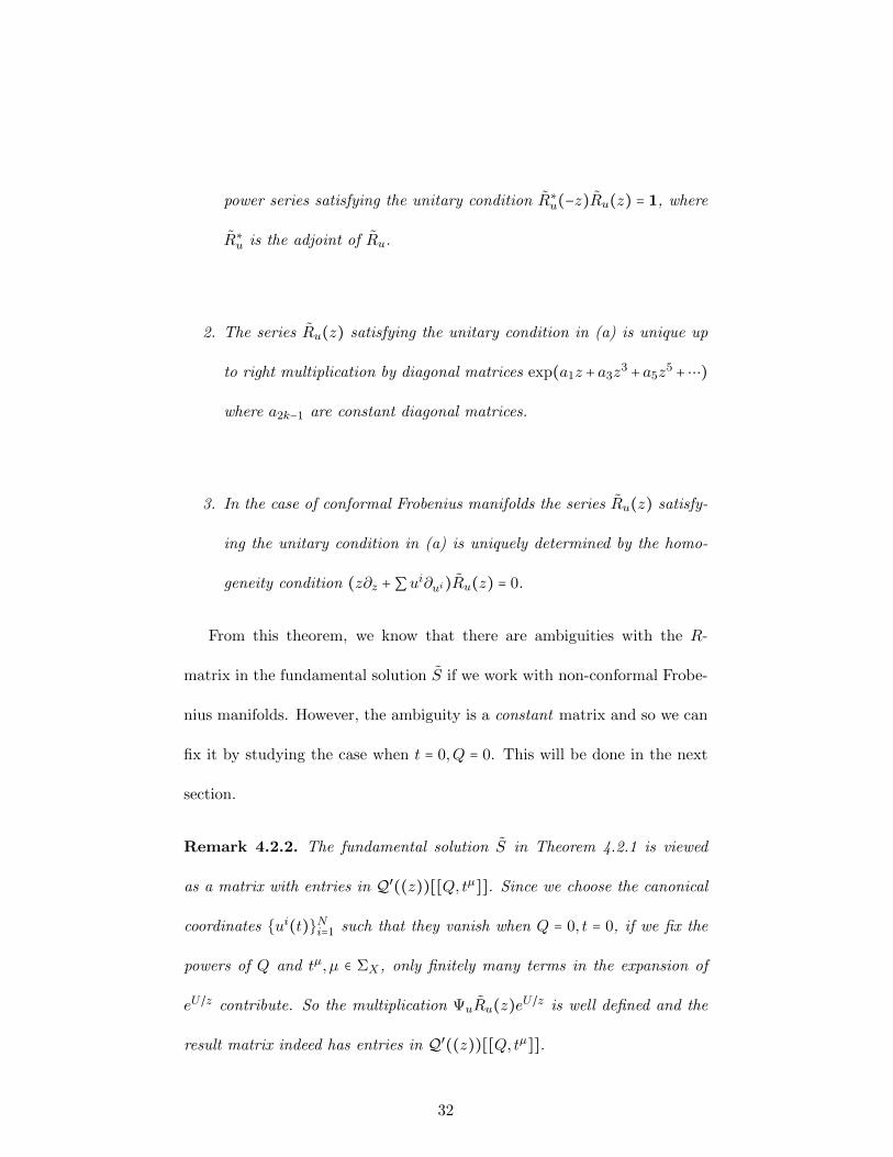
power series satisfying the unitary condition R∗u(−z)Ru(z) = 1, where

R∗u is the adjoint of Ru.

2. The series Ru(z) satisfying the unitary condition in (a) is unique up

to right multiplication by diagonal matrices exp(a1z + a3z3 + a5z

5 +⋯)

where a2k−1 are constant diagonal matrices.

3. In the case of conformal Frobenius manifolds the series Ru(z) satisfy-

ing the unitary condition in (a) is uniquely determined by the homo-

geneity condition (z∂z +∑ui∂ui)Ru(z) = 0.

From this theorem, we know that there are ambiguities with the R-

matrix in the fundamental solution S if we work with non-conformal Frobe-

nius manifolds. However, the ambiguity is a constant matrix and so we can

fix it by studying the case when t = 0,Q = 0. This will be done in the next

section.

Remark 4.2.2. The fundamental solution S in Theorem 4.2.1 is viewed

as a matrix with entries in Q′((z))[[Q, tµ]]. Since we choose the canonical

coordinates ui(t)Ni=1 such that they vanish when Q = 0, t = 0, if we fix the

powers of Q and tµ, µ ∈ ΣX , only finitely many terms in the expansion of

eU/z contribute. So the multiplication ΨuRu(z)eU/z is well defined and the

result matrix indeed has entries in Q′((z))[[Q, tµ]].

32

Remark 4.2.3. For a general abstract semi-simple Frobenius manifold de-

fined over a ring A, the expression S = ΨR(z)eU/z in Theorem 4.2.1 can

be understood in the following way. We consider the free module M =

⟨eu1/z⟩ ⊕ ⋯ ⊕ ⟨euN /z⟩ over the ring A((z))[[t1,⋯, tN ]] where t1,⋯, tN are

the flat coordinates of the Frobenius manifold. We formally define the dif-

ferential deui/z = eui/z duiz and we extend the differential to M by the product

rule. Then we have a map d ∶ M → Mdt1 ⊕ ⋯ ⊕MdtN . We consider the

fundamental solution S = ΨR(z)eU/z as a matrix with entries in M . The

meaning that S satisfies the quantum differential equation is understood by

the above formal differential.

The operator R in Theorem 4.2.1 plays a central role in the quantization

procedure. Before we move on to the quantization process, let us consider

the potential functions of the trivial field theory IH . When we use the 1-1

correspondence between ∆12i

∂∂ui

and φµ by identifying them at the origin

t = 0,Q = 0, we can use the same index i for both of the two basis. Define

the correlator ⟨⟩IHg,k to be

⟨τa1(φi1),⋯, τak(φik)⟩IHg,k =

⎧⎪⎪⎪⎪⎪⎨⎪⎪⎪⎪⎪⎩

∆g−1+k/2i ∫Mg,k

ψa11 ⋯ψakk , if i1 = i2 = ⋯ = ik = i,

0, otherwise

where a1,⋯, ak are nonnegative integers. Let

DIH = exp (∑g≥0∑k≥0

∑a1,⋯,ak≥0

∑i1,⋯,ik∈1,⋯,N

hg−1

a1!⋯ak!⟨τa1(φi1),⋯, τak(φik)⟩

IHg,k).

33

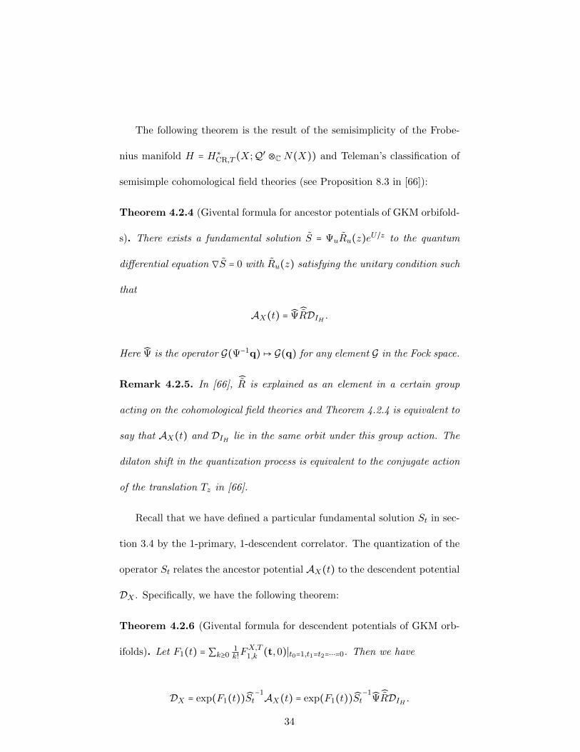
The following theorem is the result of the semisimplicity of the Frobe-

nius manifold H = H∗CR,T (X;Q′ ⊗C N(X)) and Teleman’s classification of

semisimple cohomological field theories (see Proposition 8.3 in [66]):

Theorem 4.2.4 (Givental formula for ancestor potentials of GKM orbifold-

s). There exists a fundamental solution S = ΨuRu(z)eU/z to the quantum

differential equation ∇S = 0 with Ru(z) satisfying the unitary condition such

that

AX(t) = Ψ RDIH .

Here Ψ is the operator G(Ψ−1q)↦ G(q) for any element G in the Fock space.

Remark 4.2.5. In [66], R is explained as an element in a certain group

acting on the cohomological field theories and Theorem 4.2.4 is equivalent to

say that AX(t) and DIH lie in the same orbit under this group action. The

dilaton shift in the quantization process is equivalent to the conjugate action

of the translation Tz in [66].

Recall that we have defined a particular fundamental solution St in sec-

tion 3.4 by the 1-primary, 1-descendent correlator. The quantization of the

operator St relates the ancestor potential AX(t) to the descendent potential

DX . Specifically, we have the following theorem:

Theorem 4.2.6 (Givental formula for descendent potentials of GKM orb-

ifolds). Let F1(t) = ∑k≥01k!F

X,T1,k (t,0)∣t0=1,t1=t2=⋯=0. Then we have

DX = exp(F1(t))St−1AX(t) = exp(F1(t))St

−1Ψ RDIH .

34

The proof of the relation DX = exp(F1(t))St−1At can be found in Theo-

rem 1.5.1 of [21] for the smooth case. The strategy is to use the comparison

lemma type argument to relate ψ to ψ. The proof for the orbifold case is

completely similar to the smooth case.

We should notice that althoughAX(t) depends on t, the total descendent

potential DX is indepentdent of t. For our purpose, we are more interested in

the descendent potential with primary insertions i.e the function FX,Tg,k (t, t)

defined in section 3.2. This potential function will eventually correspond

to the B-model potential under the all genus mirror symmetry studied in

[38]. The relation between FX,Tg,k (t, t) and the ancestor potential FX,Tg,k (t, t)

is even easier:

Proposition 4.2.7. For 2g − 2 + k > 0, we have the following relation

FX,Tg,k (t, t) = FX,Tg,k ([Stt]+, t).

Here we consider t = t(z) as element in H and [Stt]+ is the part of Stt

containing nonnegative powers of z.

The proof of the proposition can also be found in the proof of Theorem

1.5.1 of [21].

4.2.2 The graph sum formula

The Givental quantization formula, which involves differential operators,

can be expressed in terms of graph sums. This follows from the standard

35

correspondence between differential operators and Feynman type graph sum

formulas (see [29]). In this section, we describe a graph sum formula of

FX,Tg,k (t, t) which is equivalent to Theorem 4.2.4. By using Proposition 4.2.7,

we obtain the graph sum formula for FX,Tg,k (t, t). The graph sum formula

gives us a more explicit expression of the Givental formula. In [38], we prove

the all genus mirror symmetry for toric Calabi-Yau 3-orbifolds by expressing

both the A-model and B-model potentials as graph sums and by identifying

each term in the graph sum. We will also sketch this proof in Chapter 5.

In this subsection, every matrix expression of the corresponding linear

operator is under the basis φµ.

Given a connected graph Γ, we introduce the following notation.

1. V (Γ) is the set of vertices in Γ.

2. E(Γ) is the set of edges in Γ.

3. H(Γ) is the set of half edges in Γ.

4. Lo(Γ) is the set of ordinary leaves in Γ.

5. L1(Γ) is the set of dilaton leaves in Γ.

With the above notation, we introduce the following labels:

1. (genus) g ∶ V (Γ)→ Z≥0.

2. (marking) i ∶ V (Γ) → 1,⋯,N. This induces i ∶ L(Γ) = Lo(Γ) ∪

L1(Γ)→ 1,⋯,N, as follows: if l ∈ L(Γ) is a leaf attached to a vertex

v ∈ V (Γ), define i(l) = i(v).

36

3. (height) a ∶H(Γ)→ Z≥0.

Given an edge e, let h1(e), h2(e) be the two half edges associated to e.

The order of the two half edges does not affect the graph sum formula in

this paper. Given a vertex v ∈ V (Γ), let H(v) denote the set of half edges

emanating from v. The valency of the vertex v is equal to the cardinality of

the set H(v): val(v) = ∣H(v)∣. A labeled graph Γ = (Γ, g, i, a) is stable if

2g(v) − 2 + val(v) > 0

for all v ∈ V (Γ).

Let Γ(X) denote the set of all stable labeled graphs Γ = (Γ, g, i, a). The

genus of a stable labeled graph Γ is defined to be

g(Γ) ∶= ∑v∈V (Γ)

g(v) + ∣E(Γ)∣ − ∣V (Γ)∣ + 1 = ∑v∈V (Γ)

(g(v) − 1) + ( ∑e∈E(Γ)

1) + 1.

Define

Γg,k(X) = Γ = (Γ, g, i, a) ∈ Γ(X) ∶ g(Γ) = g, ∣Lo(Γ)∣ = k.

Let t(z) = ∑µ tµ(z)φµ.

We assign weights to leaves, edges, and vertices of a labeled graph Γ ∈

Γ(X) as follows.

1. Ordinary leaves. To each ordinary leaf l ∈ Lo(Γ) with i(l) = i ∈

37

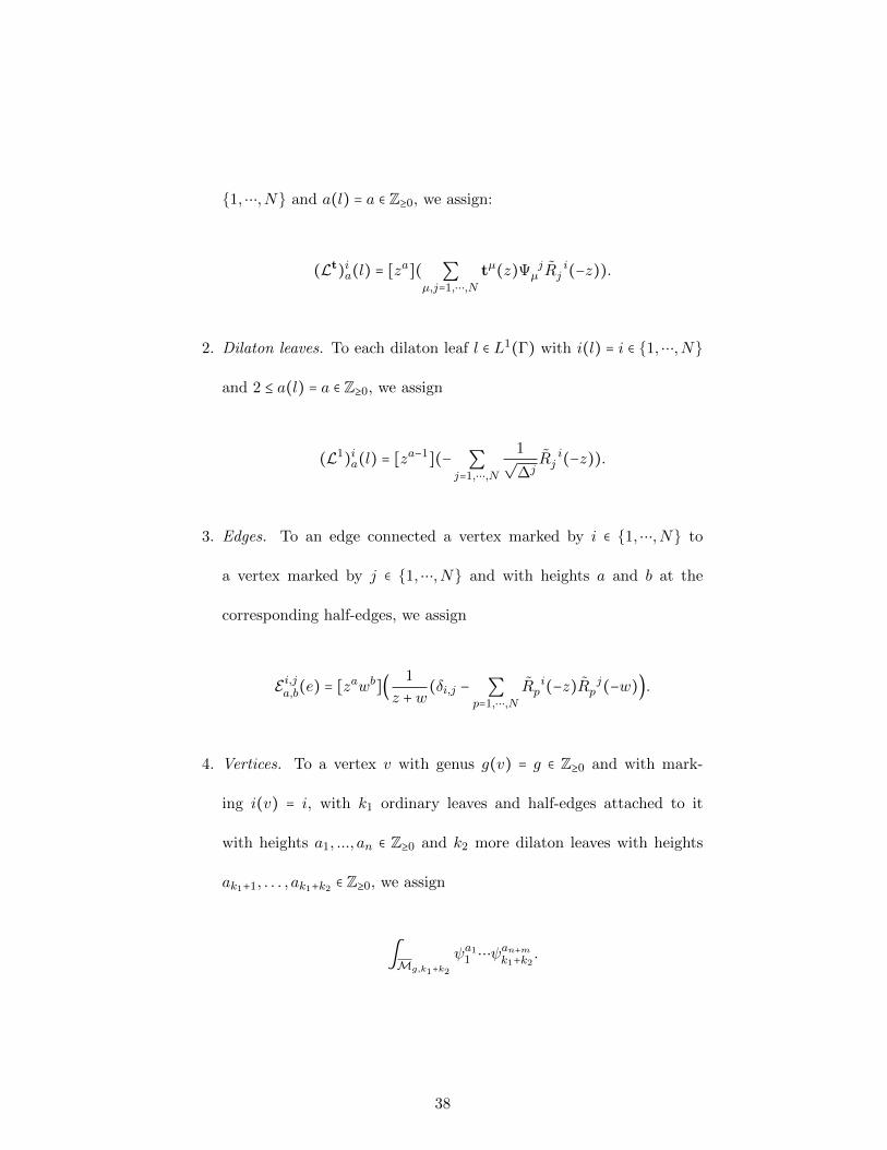
1,⋯,N and a(l) = a ∈ Z≥0, we assign:

(Lt)ia(l) = [za]( ∑µ,j=1,⋯,N

tµ(z)Ψ jµ R

ij (−z)).

2. Dilaton leaves. To each dilaton leaf l ∈ L1(Γ) with i(l) = i ∈ 1,⋯,N

and 2 ≤ a(l) = a ∈ Z≥0, we assign

(L1)ia(l) = [za−1](− ∑j=1,⋯,N

1√∆j

R ij (−z)).

3. Edges. To an edge connected a vertex marked by i ∈ 1,⋯,N to

a vertex marked by j ∈ 1,⋯,N and with heights a and b at the

corresponding half-edges, we assign

E i,ja,b(e) = [zawb]( 1

z +w (δi,j − ∑p=1,⋯,N

R ip (−z)R j

p (−w)).

4. Vertices. To a vertex v with genus g(v) = g ∈ Z≥0 and with mark-

ing i(v) = i, with k1 ordinary leaves and half-edges attached to it

with heights a1, ..., an ∈ Z≥0 and k2 more dilaton leaves with heights

ak1+1, . . . , ak1+k2 ∈ Z≥0, we assign

∫Mg,k1+k2

ψa11 ⋯ψan+mk1+k2

.

38

We define the weight of a labeled graph Γ ∈ Γ(P1) to be

w(Γ) = ∏v∈V (Γ)

(√

∆i(v))2g(v)−2+val(v)⟨ ∏h∈H(v)

τa(h)⟩g(v) ∏e∈E(Γ)

E i(v1(e)),i(v2(e))a(h1(e)),a(h2(e))

(e)

⋅ ∏l∈Lo(Γ)

(Lt)i(l)a(l)

(l) ∏l∈L1(Γ)

(L1)i(l)a(l)

(l).

Then

log(AX(t)) = ∑Γ∈Γ(X)

hg(Γ)−1w(Γ)∣Aut(Γ)∣

=∑g≥0

hg−1∑k≥0

∑Γ∈Γg,k(X)

w(Γ)∣Aut(Γ)∣

.

By Proposition 4.2.7, FX,Tg,k (t, t) can be obtained by FX,Tg,k (t, t) by change

of variables defined by the operator St(z). So in order to get the graph sum

formula for FX,Tg,k (t, t), we only need to modify the ordinary leaves:

(1)’ Ordinary leaves. To each ordinary leaf l ∈ Lo(Γ) with i(l) = i ∈

1,⋯,N and a(l) = a ∈ Z≥0, we assign:

(Lt)ia(l) = [za]( ∑µ,ν,j=1,⋯,N

tµ(z)St(z)νµΨ jν R

ij (−z)).

We define a new weight of a labeled graph Γ ∈ Γ(X) to be

w(Γ) = ∏v∈V (Γ)

(√

∆i(v))2g(v)−2+val(v)⟨ ∏h∈H(v)

τa(h)⟩g(v) ∏e∈E(Γ)

E i(v1(e)),i(v2(e))a(h1(e)),a(h2(e))

(e)

⋅ ∏l∈Lo(Γ)

(Lt)i(l)a(l)

(l) ∏l∈L1(Γ)

(L1)i(l)a(l)

(l).

39

Then

∑g≥0

hg−1∑k≥0

1

k!FX,Tg,k (t, t) = ∑

Γ∈Γ(X)

hg(Γ)−1w(Γ)∣Aut(Γ)∣

=∑g≥0

hg−1∑k≥0

∑Γ∈Γg,k(X)

w(Γ)∣Aut(Γ)∣

.

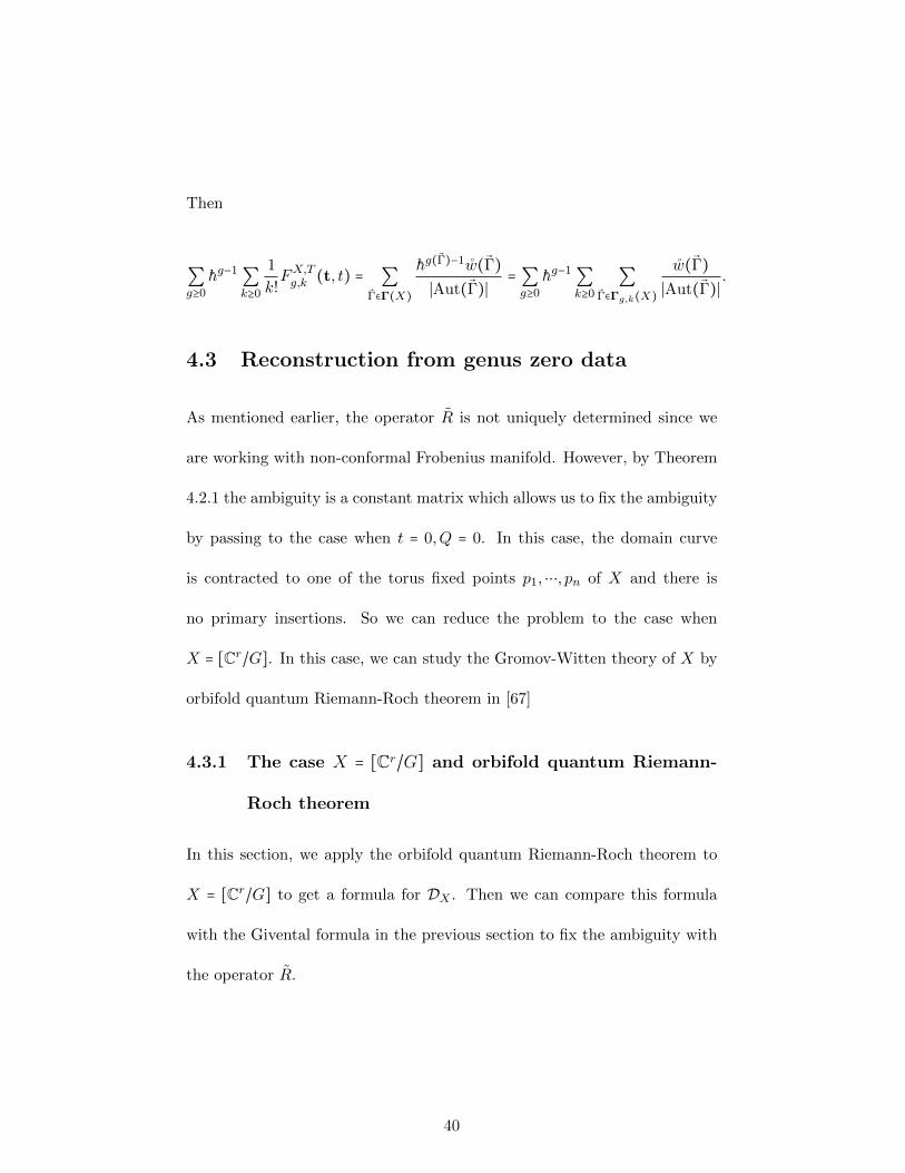
4.3 Reconstruction from genus zero data

As mentioned earlier, the operator R is not uniquely determined since we

are working with non-conformal Frobenius manifold. However, by Theorem

4.2.1 the ambiguity is a constant matrix which allows us to fix the ambiguity

by passing to the case when t = 0,Q = 0. In this case, the domain curve

is contracted to one of the torus fixed points p1,⋯, pn of X and there is

no primary insertions. So we can reduce the problem to the case when

X = [Cr/G]. In this case, we can study the Gromov-Witten theory of X by

orbifold quantum Riemann-Roch theorem in [67]

4.3.1 The case X = [Cr/G] and orbifold quantum Riemann-

Roch theorem

In this section, we apply the orbifold quantum Riemann-Roch theorem to

X = [Cr/G] to get a formula for DX . Then we can compare this formula

with the Givental formula in the previous section to fix the ambiguity with

the operator R.

40

Recall that the Bernoulli polynomials Bm(x) are defined by

tetx

et − 1= ∑m≥0

Bm(x)tmm!

.

The Bernoulli numbers are given by Bm ∶= Bm(0).

Let BG be the classifying stack of the finite group G. Then by Example

2.2.2,

IBG = ⊔(h)∈Conj(G)

[pt/C(h)]

and

H∗(IBG;C) = ⊕(h)∈Conj(G)

C1(h).

Now we consider the Chen-Ruan cohomology H∗CR(BG;Q′). For each irre-

ducible representation Vα of G, let

φα =dimVα

∣G∣ ∑(h)∈Conj(G)

χα(h−1)1(h).

Then by [50] (or by specializing the computation in Section 2.3 to the case

when r = 0), we have

φα ⋆ φα′ = δα,α′∣G∣

dimVαφα

and

⟨φα, φα′⟩BG = δα,α′ .

41

So φα is a normalized canonical basis for H∗CR(BG;Q′).

For each integer m ≥ 0 and i = 1,⋯, r, define an linear operator Aim ∶

H∗(IBG)→H∗(IBG) by

Aim(1(h)) ∶= Bm(ci(h))1(h).

Then we define the symplectic operator P (z) to be

P (z) ∶=r

∏i=1

exp(∑m≥1

(−1)mm(m + 1)

r

∑i=1

Aim+1(z

wi)m),

where wi is the torus character in the i−th tangent direction.

Let H ∶= H∗CR(BG;Q′) and we define the cohomological field theory IH

as follows. Define the genus g correlator ⟨⟩IHg,k to be

⟨τa1(φi1),⋯, τak(φik)⟩IHg,k =

⎧⎪⎪⎪⎪⎪⎨⎪⎪⎪⎪⎪⎩

( ∣G∣√∏j wj

dimVi)2g−2+k ∫Mg,k

ψa11 ⋯ψakk , if i1 = i2 = ⋯ = ik = i,

0, otherwise

where a1,⋯, ak are nonnegative integers. Let

DIH = exp (∑g≥0∑k≥0

∑a1,⋯,ak≥0

∑i1,⋯,ik∈1,⋯,∣Conj(G)∣

hg−1

a1!⋯ak!⟨τa1(φi1),⋯, τak(φik)⟩

IHg,k).

Then we have the following orbifold quantum Riemann-Roch theorem

[67]:

42

Theorem 4.3.1 (orbifold quantum Riemann-Roch theorem for X).

DX = PDIH .

Now we make the following key observation. When t = 0,Q = 0, ∆i =

∣G∣2∏j wj(dimVi)2 . This means that the Frobenius algebra H ∣t=0,Q=0 is isomorphic to

H and the isomorphism is given by

φi ↦ φi

for i = 1,⋯, ∣Conj(G)∣. On the other hand, when t = 0,Q = 0 we have

DX = AX and Ψ is trivial. So by comparing theorem 4.2.4 and theorem

4.3.1, we know that

R ij ∣t=0,Q=0 = P i

j ,

where (P ij ) is the matrix expression of P under the basis φα. Therefore

if we let αi, αj be the corresponding irreducible representation, we have

R ij ∣t=0,Q=0 =

1

∣G∣ ∑(h)∈Conj(G)

χαj(h)χαi(h−1)r

∏k=1

exp(∞

∑m=1

(−1)mm(m + 1)Bm+1(ck(h))(

z

wk)m).

(4.1)

4.3.2 The general case

In general, when t = 0,Q = 0, the domain curve is contracted to one of

the torus fixed points p1,⋯, pn. So we apply the quantum Riemann-Roch

43

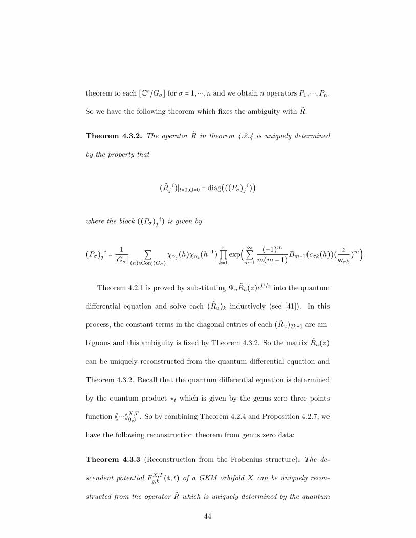
theorem to each [Cr/Gσ] for σ = 1,⋯, n and we obtain n operators P1,⋯, Pn.

So we have the following theorem which fixes the ambiguity with R.

Theorem 4.3.2. The operator R in theorem 4.2.4 is uniquely determined

by the property that

(R ij )∣t=0,Q=0 = diag(((Pσ) i

j ))

where the block ((Pσ) ij ) is given by

(Pσ) ij = 1

∣Gσ ∣∑

(h)∈Conj(Gσ)

χαj(h)χαi(h−1)r

∏k=1

exp(∞

∑m=1

(−1)mm(m + 1)Bm+1(cσk(h))(

z

wσk)m).

Theorem 4.2.1 is proved by substituting ΨuRu(z)eU/z into the quantum

differential equation and solve each (Ru)k inductively (see [41]). In this

process, the constant terms in the diagonal entries of each (Ru)2k−1 are am-

biguous and this ambiguity is fixed by Theorem 4.3.2. So the matrix Ru(z)

can be uniquely reconstructed from the quantum differential equation and

Theorem 4.3.2. Recall that the quantum differential equation is determined

by the quantum product ⋆t which is given by the genus zero three points

function ⟪⋯⟫X,T0,3 . So by combining Theorem 4.2.4 and Proposition 4.2.7, we

have the following reconstruction theorem from genus zero data:

Theorem 4.3.3 (Reconstruction from the Frobenius structure). The de-

scendent potential FX,Tg,k (t, t) of a GKM orbifold X can be uniquely recon-

structed from the operator R which is uniquely determined by the quantum

44

multiplication law and the property

(R ij )∣t=0,Q=0 = diag(((Pσ) i

j ))

where diag(((Pσ) ij )) is a constant matrix which is explicitly given by The-

orem 4.3.2.

45

Chapter 5

Application: all genus mirror

symmetry for toric

Calabi-Yau 3-orbifolds

5.1 Introduction

In this chapter, we consider the case when X is a toric Calabi-Yau 3-orbifold.

Then X contains an algebraic torus (C∗)3 as Zariski dense open subset. We

choose the torus T to be the two dimensional sub-torus of (C∗)3 which acts

trivially on Λ3TX. In this case, there exists a particularly nice duality.

This story comes from the remodeling conjecture, which is established in

[65] [8] and [9]. The remodeling conjecture can be viewed as an all genus

mirror symmetry for toric Calabi-Yau 3-orbifolds. In this conjecture, the

46

A-model higher genus potential is the open Gromov-Witten potential of X

with respect to one or several Aganagic-Vafa branes on X. The higher genus

B-model ωg,n is obtained by applying the Eynard-Orantin [32] topological

recursion to the mirror curve C of X. It is a symmetric n-form on C. When

ωg,n is expanded around certain points on C, the coefficients will give us

the open Gromov-Witten invariants of X. More than one Aganagic-Vafa

branes can be put on X depending on around which points we expend ωg,n.

The interesting thing here is that the Eynard-Orantin topological recursion

itself is motivated by matrix model theory, which was not expected to be

related to mirror symmetry at the beginning. The Eynard-Orantin theory

itself also has its own interests and can be applied to much more general

targets such as quantum curves, higher dimensional manifolds and so on.

Before we discuss the all genus mirror symmetry for X, we should notice

that one can build the genus 0 mirror symmetry for toric orbifolds of any

dimensions by using their Landau-Ginzburg mirrors, which contains a super

potential W T ∶ (C∗)r → C. Here T is the torus acting on the r−dimensional

toric orbifold. In the general toric case, the genus 0 mirror symmetry has

been studied in [40] for smooth toric varieties and in [22] for toric Deligne-

Mumford (DM) stacks. The genus 0 mirror theorem gives us an isomorphism

between the quantum cohomology ring of a toric orbifold and the Jacobi ring

of its Landau-Ginzburg mirror. So one can identify the Frobenius structures

of these two rings. In particular, the quantum differential equations in A

and B-model can be identified.

47

So far, we have two kinds of mirrors associated to a toric Calabi-Yau

3-orbifold X: the mirror curve of and the Landau-Ginzburg mirror of X. It

is natural to ask whether these two B-models are related. Let the mirror

curve C be defined by an equation H:

C = (X,Y )∣H(X,Y ) = 0 ⊂ (C∗)2.

On the Landau-Ginzburg B-model side, we have a super potential

W T ∶ (C∗)3 → C

with

W T =H(X,Y )Z − u1 logX − u2 logY,

where H∗(BT ;C) = C[u1, u2]. This explicit expression of W T gives us the

relation between the mirror curve of and the Landau-Ginzburg mirror of X.

If we view X ∶ C → C∗ as a super potential on C, then the structure of the

mirror curve gives us a singularity theory on C. The above relation can be

viewed as the dimensional reduction from the singularity theory on (C∗)3

to the singularity theory on C.

The remodeling conjecture, which relates the formal generating functions

of higher genus Gromov-Witten invariants of X to the analytic symmetric

forms on C, seems to be mysterious at the beginning. The structure behind

this conjecture is that both A-model and B-model higher genus potentials

48

can be realized as quantizations on on two isomorphic semisimple Frobenius

manifolds. With this structure in mind, the remodeling conjecture becomes

natural to understand. The genus 0 mirror theorem identifies the Frobenius

structure of the quantum cohomology of X and the Frobenius structure

of the Jacobi ring of W T . By the dimensional reduction, the Frobenius

structure on the Landau-Ginzburg B-model reduces to the structure on the

mirror curve C. In particular, we can consider the fundamental solution to

the B-model quantum differential equation and the B-model R−matrix. The

A-model and B-model R−matrices are then identified by comparing the am-

biguities in Theorem 4.2.1. The A-model higher genus potential is obtained

by Givental quantization formula developed in the previous chapters. The

B-model higher genus potential is obtained by the Eynard-Orantin topolog-

ical recursion on C. The bridge relating these two potentials is the graph

sum formula, which is equivalent to both the quantization formula and the

recursive formula. Finally, the remodeling conjecture is proved by identify-

ing the A-model and B-model graph sums, which is a direct result of the

identification of A-model and B-model R−matrices.

The proof of the remodeling conjecture for general toric Calabi-Yau 3-

orbifolds is in [38]. In the following sections, we illustrating the strategy of

the proof and ideas behind the proof. In particular, we will see that the

Givental quantization formula developed in the previous chapters gives the

key to relate the A-model and B-model higher genus potentials.

49

5.2 A-model geometry

In this section, we discuss the basis properties of toric Calabi-Yau 3-orbifolds.

Then we apply the Givental quantization formula to this special case to

study the higher genus Gromov-Witten potentials of toric Calabi-Yau 3-

orbifolds.

5.2.1 Toric Calabi-Yau 3-orbifolds

Let X be a semi-projective toric Calabi-Yau 3-orbifold defined by a stacky

fan Σ = (N,Σ, ρ) [7]. Then X contains the algebraic torus T = (C∗)3 as

Zariski dense open subset, and N = Hom(C∗,T) ≅ Z3. We assume that

there is at least one T−fixed point on X. Let M = Hom(T,C∗) = N∨ be

the group of irreducible characters of T. The course moduli space of X

is the simplicial toric variety X ′Σ defined by the simplicial fan Σ, and the

canonical divisor KX′

Σof X ′

Σ is trivial. Let X ′0 ∶= SpecH0(X ′,OX′) be the

affinization of X ′. Then X ′0 is an affine Gorenstein toric variety defined by

a cone σ0 ⊂ NR ∶= N ⊗R R.

In this case, we choose our torus T to be the 2-dimensional sub-torus of

T such that T acts trivially on Λ3TX. Then T ≅ T × C∗ and N ≅ N ′ × Z,

where N ′ = Hom(C∗, T ) ≅ Z2. Then σ0 is the cone over P × 1 ⊂ N ′R × R,

where P is a convex polytope in N ′R with vertices in N ′. There is a one-

to-one correspondence between the T -fixed points p1,⋯, pn in X and the

3-dimensional cones in Σ. Let σ ∈ Σ(3) be a 3-dimensional cone and let Nσ

50

be the sublattice spanned by σ. Then Gσ = N/Nσ is a finite abelian group

and there is a one-to-one correspondence between elements in Box(σ) ⊂ N

and elements in Gσ:

b ∈ Box(σ)↦ b +Nσ ∈ N/Nσ = G.

The cone σ defines an affine toric Calabi-Yau 3-fold Xσ ≅ [C3/Gσ] ⊂ X

which is a local neighborhood of pσ.

5.2.2 A-model topological string

Recall that in Section 3.2, we have defined the double correlator

⟪t(ψ1),⋯, t(ψk)⟫X,Tg,k ∶=∞

∑s=0∑β∈E

Qβ

s!⟨t(ψ1),⋯, t(ψk), t,⋯, t⟩X,Tg,k+s,β.

Then we studied the quantization formula for this descendent potential.

In order to apply this general formula to the remodeling conjecture, we

need to slightly modify this potential. In this subsection, we describe these

modifications which are all straightforward.

First, we need to restrict the primary insertion t to the subspaceH2CR(X;C),

where the corresponding coordinates ti are called kahler parameters. Sec-

ond, note that H2(X;Z) is dual to H2(X;Z), the numner Novikov variables

Qi are equal to the rank of H2(X;Z). When we deal with the quantum

cohomology of X, we can use the divisor equation to pull out the H2(X;C)

part of t to get the factor eti in front of the correlator. The Novikov variable

51

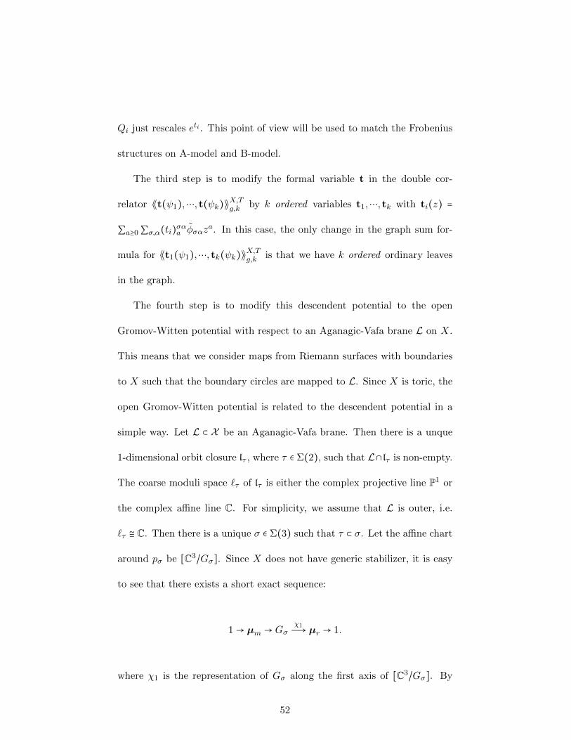
Qi just rescales eti . This point of view will be used to match the Frobenius

structures on A-model and B-model.

The third step is to modify the formal variable t in the double cor-

relator ⟪t(ψ1),⋯, t(ψk)⟫X,Tg,k by k ordered variables t1,⋯, tk with ti(z) =

∑a≥0∑σ,α(ti)σαa φσαza. In this case, the only change in the graph sum for-

mula for ⟪t1(ψ1),⋯, tk(ψk)⟫X,Tg,k is that we have k ordered ordinary leaves

in the graph.

The fourth step is to modify this descendent potential to the open

Gromov-Witten potential with respect to an Aganagic-Vafa brane L on X.

This means that we consider maps from Riemann surfaces with boundaries

to X such that the boundary circles are mapped to L. Since X is toric, the

open Gromov-Witten potential is related to the descendent potential in a

simple way. Let L ⊂ X be an Aganagic-Vafa brane. Then there is a unque

1-dimensional orbit closure lτ , where τ ∈ Σ(2), such that L∩ lτ is non-empty.

The coarse moduli space `τ of lτ is either the complex projective line P1 or

the complex affine line C. For simplicity, we assume that L is outer, i.e.

`τ ≅ C. Then there is a unique σ ∈ Σ(3) such that τ ⊂ σ. Let the affine chart

around pσ be [C3/Gσ]. Since X does not have generic stabilizer, it is easy

to see that there exists a short exact sequence:

1→ µm → Gσχ1Ð→ µr → 1.

where χ1 is the representation of Gσ along the first axis of [C3/Gσ]. By

52

localization, in the fixed loci the domain curve degenerates into a closed

curve with several disks attaching to it. The disks are mapped to lτ and the

maps are of the form z → zd for some d ∈ Z>0 called the winding number.

The closed part of the curve contributes the descendent Gromov-Witten

invariant with descendent markings the nodes connecting the disks. These

descendent markings are of course mapped to pσ. So we only need to replace

the formal variables (ti)σαa in ⟪t1(ψ1),⋯, tk(ψk)⟫X,Tg,k by the disk functions

ξσ,αa (Xi), where Xi is a formal variable and ξσ,αa (Xi) is a power series of

Xi. The disk function ξσ,αa (Xi) is the contribution of the i−th disk and the

power of Xi records the winding number of the i−th disk. The function

ξσ,αa (Xi) is an explicit function and the reader is referred to [36] for the

expression of ξσ,αa (Xi). One should notice that if m > 1, lτ is gerby. So in

the definition of open Gromov-Witten invariants with respective to L, we

need to input the additional data of monodromies at infinity of the disks

besides the data of winding numbers. Therefore, the disk function ξσ,αa (Xi)

is in fact H∗CR(BZm)-valued.

The last step is to introduce the framing. Consider the affine chart

[C3/Gσ] in the fourth step. Recall that there exists a short exact sequence:

1→ µm → Gσχ1Ð→ µr → 1.

where χ1 is the representation of Gσ along the first axis of [C3/Gσ]. Let

w1,w2,w3 be the three torus weights along the three axes of [C3/Gσ] respec-

53

tively. Then we do the following specialization:

w1 ↦1

rv = w1v, w2 ↦

s + rfrm

v = w2v, w3 ↦−s − rf −m

rmv = w3v.

with f an integer. Introducing the framing f is equivalent to the following.

Consider the subtorus

Tf T

which corresponds to the character v above. Then we project the open

Gromov-Witten potential to the fractional field of H∗tw(BTf ;C). Then as

priori, our open Gromov-Witten potential is defined over C(v). But since

our primary insertions are restricted toH2tw(X;C), the open Gromov-Witten

potential is in fact independent of v.

After the above five steps, we obtain an open Gromov-Witten potential

FX ,(L,f)g,n (t;X1, . . . ,Xn) from the descendent potential ⟪t(ψ1),⋯, t(ψk)⟫X,Tg,k .

We still have the graph sum formula for FX ,(L,f)g,n (t;X1, . . . ,Xn) as in Section

4.2.2. The difference is that we have k ordered ordinary leaves and the

formal variables (ti)σαa are replaced by the disk functions ξσ,αa (Xi). This

replacement only changes the ordinary leaves in the graph sum formula.

54

5.3 B-model geometry

5.3.1 Mirror curve and dimensional reduction of the Landau-

Ginzburg model

Recall that in Section 5.2.1, we have a polytope P in N ′R with vertices in

N ′. If we choose an isomorphism N ′ ≅ Z2, then the mirror curve is defined

by

(X,Y ) ∈ (C∗)2 ∶H(X,Y ) = 0

where

H(X,Y ) =XrY −s−rf + Y m + 1 +p

∑a=1

qaXmaY na−maf

P∩Z2 = (r,−s), (0,m), (0,0)∪(ma, na) ∶ a = 1, . . . , p, p = dimCH2CR(X ).

Here q1,⋯, qp are complex parameters on B-model. If we let t1,⋯, tp be

coordinates of H2CR(X ), which means that t1,⋯, tp are Kahler parameters

on A-model. Then q1,⋯, qp and t1,⋯, tp are related by closed mirror maps

[35] [38].

On the other hand, The T -equivariant mirror of X is a Landau-Gizburg

model ((C∗)3,W T ), where W T ∶ (C∗)3 → C is the T -equivariant superpo-

tential

W T =H(X,Y )Z − logX

55

which is multi-valued. The differential

dW T = ∂WT

∂XdX + ∂W

T

∂YdY + ∂W

T

∂ZdZ = ZdH +HdZ − dX

X

is a well-defined holomorphic 1-form on (C∗)3.

We have

∂W T

∂X(X,Y,Z) = Z

∂H

∂X(X,Y ) − 1

X

∂W T

∂Y(X,Y,Z) = Z

∂H

∂Y(X,Y )

∂W T

∂Z(X,Y,Z) = H(X,Y )

Therefore,

∂W T

∂X= 0,

∂W T

∂Y= 0,

∂W T

∂Z= 0

are equivalent to

H(X,Y ) = 0,∂H

∂X(X,Y ) = − 1

Z

∂x

∂X,

∂H

∂Y(X,Y ) = 0

where x = − lnX. Therefore, the critical points of W T (X,Y,Z), which are

zeros of the holomorphic differential dW T on (C∗)3, can be identified with

the critical points of p, which are zeros of the holomorphic differential

dx = −dXX

56

on the mirror curve

Σq = (X,Y ) ∈ (C∗)2 ∶H(X,Y ) = 0.

Define IΣ ∶= (σ,α) ∶ σ ∈ Σ(3), α ∈ G∗σ. Then there is a bijection between

the zeros of dW T and the set IΣ. Let Pσ,α ∈ (C∗)3 be the zero of dW T

associated to (σ,α) ∈ IΣ and let pσ,α ∈ Σq be the corresponding critical

points of x on Σq.

The Jacobian ring of W T is

Jac(W T ) ∶= C[X,X−1, Y, Y −1, Z,Z−1]⟨∂WT

∂X , ∂WT

∂Y , ∂WT

∂Z ⟩≅HB ∶= C[X,X−1, Y, Y −1]

⟨H(X,Y ),−Y ∂H∂Y (X,Y )⟩

There is pairing on Jac(W T ):

(f, g) ∶= −1

(2π√−1)3 ∫∣dWT ∣=ε

fgdx ∧ dy ∧ dz∂WT

∂x∂WT′

∂y∂WT

∂z

where x = − lnX,y = − lnY, z = − lnZ.

5.3.2 The Liouville form

Let

λ = ydx.

be the Liouville form on C2. Then dλ = −dx ∧ dy. Let

Φ ∶= λ∣Σq ,

57

5.3.3 Lefshetz thimbles

Around critical points pσ,α of x ∶ Σq → C, we have have

x = uσ,α + ζ2

y = vσ,α +∞

∑d=1

hσ,αd ζd

where

hσ,α1 =¿ÁÁÀ 2

d2xdy2 (vσ,α)

Let Γσ,α be the Lefshetz thimble of the superpotential x ∶ Σq → C such that

x(Γσ,α) = uσ,α + R≥0. Then Γσ,α ∶ (σ,α) ∈ IΣ is a basis of the relative

homology group H1(Σq,x≫ 0).

5.3.4 Differentials of the second kind

Let B(p1, p2) be the fundamental normalized differential of the second kind

on Σq (see e.g. [33]), where Σq is the compactification of Σq. It is also called

the Bergman kernel in [32].

Remark 5.3.1. The compactification of Σq is a little bit subtle. Recall that

we have a polytope P which appears in the definition of X and the equation

H(X,Y ) of the mirror curve. The polytope P determines a toric surface S

together with an ample line bundle L on S. The function H(X,Y ) extends

uniquely to a section of L and the zero locus of this section in S gives us the

compactification of Σq (see [38] for more details).

58

Following [31], given α = 1,2 and d ∈ Z≥0, define

dξσ,α,d(p) ∶= (2d − 1)!!2−dResp′→pσ,αB(p, p′)ζ−2d−1σ,α .

Then dξσ,α,d satisfies the following properties.

1. dξσ,α,d is a meromorphic 1-form on Σq with a single pole of order 2d+2

at pσ,α.

2. In local coordinate ζ =√x − uσ,α near pσ,α,

dξσ,α,d = (−(2d + 1)!!2dζ2d+2

+ f(ζ))dζ,

where f(ζ) is analytic around pσ,α. The residue of dξσ,α,d at pσ,α is

zero, so dξσ,α,d is a differential of the second kind.

The meromorphic 1-form dξσ,α,d is characterized by the above properties;

dξσ,α,d can be viewed as a section in H0(Σq, ωΣq((2d + 2)pσ,α)).

Define

ξσ,α,k ∶= (−1)k( ddx

)k−1(dξσ,α,0dx

) = (X d

dX)k−1(Xdξσ,α,0

dX), (5.1)

which is a meromorphic function on Σq. We also define dξσ,α,0 ∶= dξσ,α,0.

Then we have the following lemma (see [36])

59

Lemma 5.3.2.

dξσ,α,k = dξσ,α,k −k−1

∑i=0

∑(ρ,β)∈IΣ

Bσ,α,ρ,βk−1−i,0dξρ,β,i.

where Bσ,α,βk−1−i,0 is defined in Section 5.3.7.

5.3.5 Oscillating integrals and the B-model S-matrix

Given (σ,α) ∈ IΣ, there exists Γσ,α ∈H3((C∗)3,R(WT

z ≪ 0;Z) such that

Iσ,α ∶= ∫Γσ,α

eWT

zdX

X

dY

Y

dZ

Z= 2π

√−1z∫

Γσ,αe−x/zΦ

where Φ = ydx. There exists a differential operator Dσ,α on the closed

string moduli such that the flat basis φσ,α corresponds to Dσ,αWT under

the isomoprhism H∗CR,T (X) ≅ Jac(W T ). Then for any Γ ∈H1(Σq,x ≥ 0),

∫Γe−x/zDσ′,α′Φ = ∑

(σ,α)∈IΣ

Ψ σ,ασ′,α′ ∫

Γe−x/z

dξσ,α,0√−2

Define

S σ,ασ′,α′ = ∫

Γσ,αe−x/zDσ,αΦ

The matrix S plays the role of the fundamental solution of the B-model

quantum differential equation.

60

5.3.6 The f-matrix and the B-model R-matrix

Let

f σ,αρ,δ (u) = e

uuσ,α

2√πu∫

Γσ,αe−uxdξρ,δ,0

and let

R σ,αρ,δ (z) = f σ,α

ρ,δ (−1

z)

Then by [38, 39], we have the following asymptotic expansion

S σ,ασ′,α′ =

√−2π

z(ΨR) σ,α

σ′,α′ e−uα,σ/z.

5.3.7 The Eynard-Orantin topological recursion and the B-

model graph sum

Let ωg,n be defined recursively by the Eynard-Orantin topological recursion

[32]:

ω0,1 = 0, ω0,2 = B(p1, p2).

When 2g − 2 + n > 0,

ωg,n(p1, . . . , pn) = ∑(σ,α)∈IΣ

Resp→pσ,α∫ pξ=pB(pn, ξ)

2(Φ(p) −Φ(p)(ωg−1,n+1(p, p, p1, . . . , pn−1)

+ ∑g1+g2=g

∑I∪J=1,...,n−1

I∩J=∅

ωg1,∣I ∣+1(p, pI)ωg2,∣J ∣+1(p, pJ)

Following [30], the B-model invariants ωg,n are expressed in terms of

graph sums. Given a labeled graph Γ ∈ Γg,n(X ) with Lo(Γ) = l1, . . . , ln,

61

we define its weight to be

wB(Γ) = (−1)g(Γ)−1+n ∏v∈V (Γ)

(hi(v)1√−2

)2−2g−val(v)

⟨ ∏h∈H(v)

τk(h)⟩g(v) ∏e∈E(Γ)

Bi(v1(e)),i(v2(e))k(e),l(e)

⋅n

∏j=1

1√−2dξi(lj)

k(lj)(Yj) ∏

l∈L1(Γ)

(− 1√−2

)hi(l)k(l)

.

Here, for any i, j ∈ IΣ,

B(p1, p2) = ( δi,j

(ζi − ζj)2+ ∑k,l∈Z≥0

Bi,jk,lζ

ki ζ

lj)dζidζj .

We define

Bi,jk,l =

(2k − 1)!!(2l − 1)!!2k+l+1

Bi,j2k,2l. (5.2)

And we define

hik = 2(2k − 1)!!hi2k−1.

We have the following property for Bi,jk,l:

Bi,jk,l = [u−kv−l]

⎛⎝uv

u + v (δi,j − ∑γ∈IΣf iγ(u)f jγ(v))

⎞⎠

= [zkwl]⎛⎝

1

z +w (δi,j − ∑γ∈IΣ

f iγ(1

z)f jγ(

1

w))

⎞⎠.

In our notation [30, Theorem 3.7] is equivalent to:

Theorem 5.3.3 (Dunin-Barkowski–Orantin–Shadrin–Spitz [30]). For 2g −

2 + n > 0,

ωg,n = ∑Γ∈Γg,n(X )

wB(Γ)∣Aut(Γ)∣

.

62

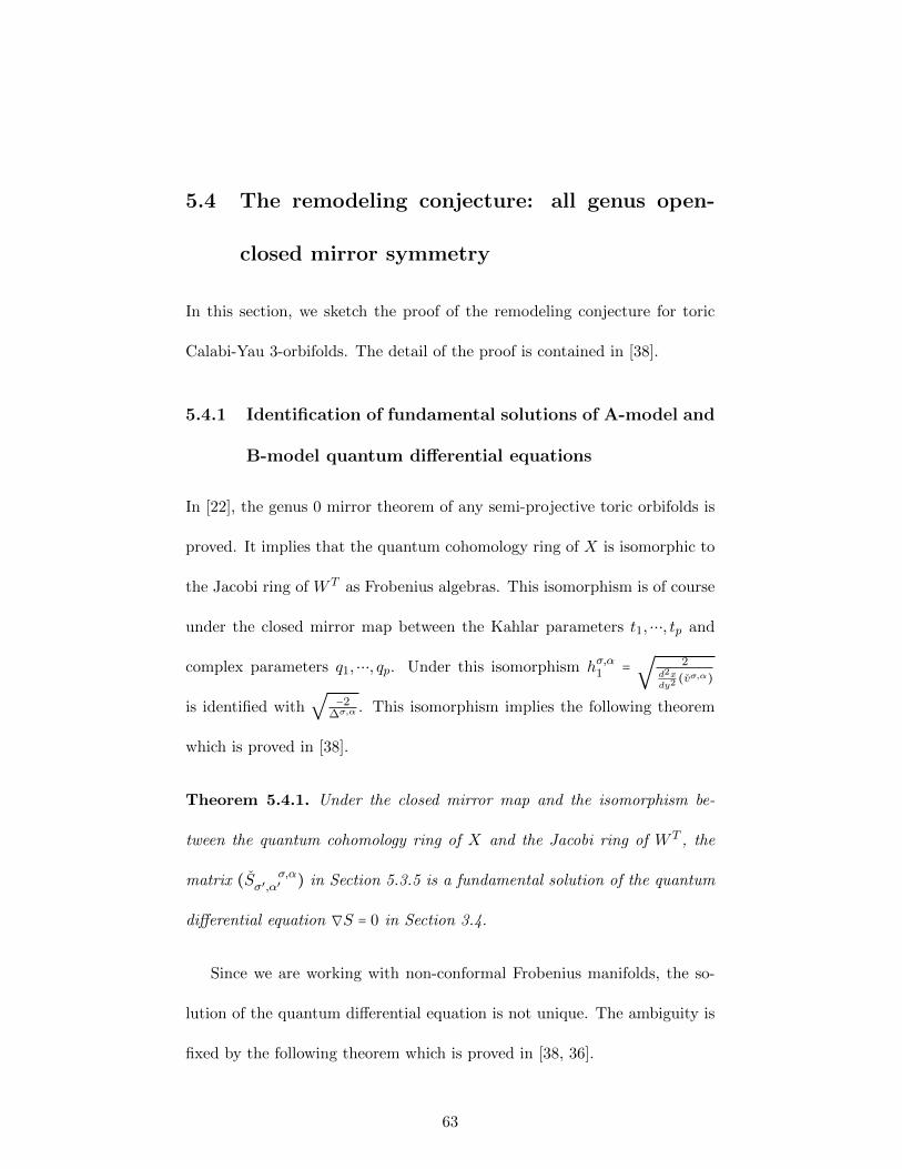
5.4 The remodeling conjecture: all genus open-

closed mirror symmetry

In this section, we sketch the proof of the remodeling conjecture for toric

Calabi-Yau 3-orbifolds. The detail of the proof is contained in [38].

5.4.1 Identification of fundamental solutions of A-model and

B-model quantum differential equations

In [22], the genus 0 mirror theorem of any semi-projective toric orbifolds is

proved. It implies that the quantum cohomology ring of X is isomorphic to

the Jacobi ring of W T as Frobenius algebras. This isomorphism is of course

under the closed mirror map between the Kahlar parameters t1,⋯, tp and

complex parameters q1,⋯, qp. Under this isomorphism hσ,α1 =√

2d2xdy2 (vσ,α)

is identified with√

−2∆σ,α . This isomorphism implies the following theorem

which is proved in [38].

Theorem 5.4.1. Under the closed mirror map and the isomorphism be-

tween the quantum cohomology ring of X and the Jacobi ring of W T , the

matrix (S σ,ασ′,α′ ) in Section 5.3.5 is a fundamental solution of the quantum

differential equation ∇S = 0 in Section 3.4.

Since we are working with non-conformal Frobenius manifolds, the so-

lution of the quantum differential equation is not unique. The ambiguity is

fixed by the following theorem which is proved in [38, 36].

63

Theorem 5.4.2.

S∣t=0,Q=0 = S∣q=0

where S is the A-model fundamental solution.

In the proof of this theorem, the A-model fundamental solution is com-

puted by Theorem 4.3.2.

By the above two theorems and and Theorem 4.2.1 we can identify the

A-model and B-model R−matrices.

R(z) = R(z).

Here we use the asymptotic expansion

S σ,ασ′,α′ =

√−2π

z(ΨR) σ,α

σ′,α′ e−uα,σ/z.

5.4.2 Identification of graph sums

In this subsection, we prove the remodeling conjecture by identifying the

graph sums on A-model and B-model. This shows that the A-model and

B-model higher genus potentials are quantizations on two isomorphic semi-

simple Frobenius manifolds.

Define the A-model graph weight wA(Γ) to be the graph weight w(Γ) in

Section 4.2.2 after the modification described in Section 5.2.2. For l = 1,⋯, k

64

and i ∈ IΣ, let

uil(z) = ∑a≥0

(ul)iaza ∶= ∑µ,ν=1,⋯,N

(∑b≥0

ξµb (Xl)zb)St(z)νµΨ iν .

The identification R(z) = R(z) implies the following theorem:

Theorem 5.4.3. For any Γ ∈ Γg,k(X),

wB(Γ)∣ 1√

−2dξi,a(pl)=(ul)τa

= (−1)g(Γ)−1+kwA(Γ),

under the closed mirror map.

Proof. 1. Vertex. By the discussion in Section 5.4.1, hi1 =√

−2∆i for any

i ∈ IΣ. So in the model vertex term,hi1√−2

=√

1∆i . Therefore the

B-model vertex matches the A-model vertex.

2. Edge. By the property for Bi,ja,b,

Bi,ja,b = [u−av−b]

⎛⎝uv

u + v (δi,j − ∑γ∈IΣf iγ(u)f jγ(v))

⎞⎠

= [zawb]⎛⎝

1

z +w (δi,j − ∑γ∈IΣ

f iγ(1

z)f jγ(

1

w))

⎞⎠.

Therefore, the identification R(z) = R(z) = (f ij(−1z )) gives us

Bi,ja,b = E

i,ja,b.

3. Ordinary leaf. By Lemma 5.3.2, we have the following expression for

65

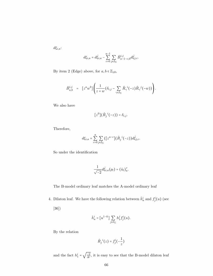
dξi,a:

dξi,a = dξi,a −a−1

∑c=0∑j∈IΣ

Bi,ja−1−c,0dξj,c.

By item 2 (Edge) above, for a, b ∈ Z≥0,

Bi,ja,b = [zawb]

⎛⎝

1

z +w (δi,j − ∑γ∈IΣ

R iγ (−z)R j

γ (−w))⎞⎠.

We also have

[z0](R ij (−z)) = δi,j .

Therefore,

dξi,a =a

∑c=0∑j∈IΣ

([za−c](R ij (−z))dξj,c.

So under the identification

1√−2dξi,a(pl) = (ul)τa.

The B-model ordinary leaf matches the A-model ordinary leaf

4. Dilaton leaf. We have the following relation between hia and f ij(u) (see

[36])

hia = [u1−k] ∑j∈IΣ

hj1fij(u).

By the relation

R ij (z) = f ij(−

1

z)

and the fact hi1 =√

−2∆i , it is easy to see that the B-model dilaton leaf

66

matches the A-model dilaton leaf.

Theorem 5.4.3 almost proves the remodeling conjecture. The only thing

remaining is to expand dξi,a(pl) at suitable points on Σq to recover the

information of uil(z) = ∑a≥0(ul)iaza = ∑µ,ν=1,⋯,N(∑b≥0 ξµb (Xl)zb)St(z)νµΨ i

ν .

We sketch this process now and the details are contained in [36, 38].

Recall that our Aganagic-Vafa brane lies at lτ which is a Zm gerbe and

the disk functions ξµa (Xl), l = 1,⋯, k, µ ∈ IΣ are H∗CR(BZm)-valued. On the

B-model side, there are m punctures p1,⋯, pm of the mirror curve Σq with

X(p1) = ⋯ = X(pm) = 0. Let D` be an open neighborhood of p` ∈ X−1(0),

` = 0, . . . ,m − 1 such that the restriction

X` ∶D` →Dδ = X ∈ C ∶ ∣X ∣ < δ,

gives an isomorphism. Define

ρ`1,...,`n ∶= (X`1)−1 ×⋯ × (X`n)−1 ∶ (Dδ)n →D`1 ×⋯ ×D`n ⊂ (Σq)n.

Define

ψ` ∶=1

m

m−1

∑k=0

ω−k`m 1 km, ` = 0,1, . . . ,m − 1,

where ωm = e2π√−1/m and H∗

CR(BZm) =⊕m−1k=0 C1 k

mis the natural decompo-

67

sition with respect to the components of IBZm. Let

dξi,a(X ′l) = ∑

`∈Zm(∫

X′

l

0(ρ`)∗(dξi,a))ψ`.

The reason why we use the notation X ′l is that there is an open mirror map

[35, 38] U ∶ (X1,⋯,Xk) ↦ (X ′1,⋯,X ′

k) where (X1,⋯,Xk) are the formal

variables on A-model recording the winding numbers. The following lemma

is proved in [38]

Lemma 5.4.4. Under the open mirror map, we have

(ul)τa(Xl) =1

∣Gσ ∣√−2dξi,a(X ′

l).

For 2g − 2 + k > 0, define

Wg,n(q;X ′1, . . . ,X

′k) ∶= ∑

`1,...,`k∈Zm∫

X′

1

0⋯∫

X′

k

0(ρ`1,...,`kq )∗ωg,k ⋅ ψ`1 ⊗⋯⊗ ψ`k ,

which takes values in H∗CR(Bµm;C)⊗k. Combining Theorem 5.4.3 and Lem-

ma 5.4.4, we finally obtain the following theorem

Theorem 5.4.5 (All genus open-closed mirror symmetry). Under the open

and closed mirror maps,

Wg,k(q,X ′1, . . . ,X

′k) = (−1)g−1+k∣Gσ ∣kFX,(L,f)g,k (t;X1, . . . ,Xk).

for 2g − 2 + k > 0.

68

Remark 5.4.6. 1. For (g, k) = (0,1), (0,2), one can still obtain the

above theorem of mirror symmetry by studying the genus 0 data di-

rectly, see [35, 36, 38].

2. One can also generalized the above theorem to the case in which we

have several Aganagic-Vafa branes (outer or inner).

3. By taking the oscillating integral of ωg,k over suitable Lefschetz thim-

bles, one can obtain the descendent version of the above theorem: the

oscillating integral of ωg,k equals to the descendent potential of X, see

[38].

5.4.3 Generalization to the multi-branes case

Theorem 5.4.5 can be easily generalized to the case when several Aganagic-

Vafa branes are put in X. In order to do this, the most convenient way

is to consider the open Gromov-Witten potential before the introduction

of framing and meanwhile consider the general Landau-Ginzburg B-model

which we will introduce below.

The general T -equivariant Landau-Ginzburg mirror of X contains a su-

per potential

W T =H(X,Y )Z − u1 logX − u2 logY

where u1, u2 span H2(BT,C).

69

For the mirror curve of X, instead of considering the framed mirror

curve, we consider the curve defined by

(X,Y ) ∈ (C∗)2 ∶H(X,Y ) = 0,

where

H(X,Y ) =XrY −s + Y m + 1 +p

∑a=1

qaXmaY na .

Then we consider the meromorphic function x = u1x+u2y instead of x. With

this definition, the dimensional reduction process still works and we get a

B-model higher genus potential ωg,k which depends on u1, u2.

By specializing u1, u2 to some multiples of v (which is equivalent to

introducing the subtorus Tf T ), we get a particular x which depends on

the framing f . The advantage of this point of view is that it is convenient to

use different local coordinates on the mirror of X to expand ωg,k. These local

coordinates correspond to the Aganagic-Vafa branes and the framing of X.

So for each brane L and each framing f , we get a corresponding x and we

use this particular x to expand those variables in ωg,k which correspond to

the boundary circles mapping to L. After this expansion, we get a B-model

potential Wg,k(q,X ′1, . . . ,X

′k) and the we have a generalization of Theorem

5.4.5 (see [38] for more details).

70

Bibliography

[1] D. Abramovich, B. Fantechi, Orbifold techniques in degeneration for-

mulas, arXiv:1103.5132.

[2] D. Abramovich, T. Graber, A. Vistoli, Algebraic orbifold quantum prod-

ucts, Orbifolds in mathematics and physics (Madison, WI, 2001), 1–24,

Contemp. Math., 310, Amer. Math. Soc., Providence, RI, 2002.

[3] D. Abramovich, T. Graber, A. Vistoli, Gromov-Witten theory of

Deligne-Mumford stacks, Amer. J. Math. 130 (2008), no. 5, 1337–1398.

[4] M. Aganagic, A. Klemm, M. Marino, C. Vafa, The topological vertex,

Comm. Math. Phys. 254 (2005), no. 2, 425–478.

[5] M. Aganagic, A. Klemm, C. Vafa, Disk instantons, mirror symmetry

and the duality web, Z. Naturforsch. A 57 (2002), 1–28.

[6] M. Aganagic, C. Vafa, Mirror symmetry, D-branes and counting holo-

morphic discs, arXiv:hep-th/0012041.

[7] L. Borisov, L. Chen, G. Smith, The orbifold Chow ring of toric Deligne-

Mumford stacks, J. Amer. Math. Soc. 18 (2005), no. 1, 193–215.

71

[8] V. Bouchard, A. Klemm, M. Marino, S. Pasquetti, Remodeling the B-

model, Comm. Math. Phys. 287 (2009), no. 1, 117–178.

[9] V. Bouchard, A. Klemm, M. Marino, S. Pasquetti, Topological open

strings on orbifolds, Comm. Math. Phys. 296 (2010), no. 3, 589–623.

[10] M. Bershadsky, A. Radul, Conformal field theories with additional Zn

symmetry, Int. J. Mod. Phys. A 02, (1987), 165.

[11] V. Bouchard, A. Catuneanu, O. Marchal, P. Su lkowski, The remodeling

conjecture and the Faber-Pandharipande formula, Lett. Math. Phys.

103 (2013), 59–77.

[12] V. Bouchard, D.H. Serrano, X. Liu, M. Mulase, Mirror symmetry for

orbifold Hurwitz numbers, J. Differential Geom. 98 (2014), no. 3, 375–

423.

[13] A. Brini, Open topological strings and integrable hierarchies: Remodel-

ing the A-model, Comm. Math. Phys. 312 (2012), no. 3, 735–780.

[14] S. Cecotti, C. Vafa, Massive orbifolds, Mod. Phys. Lett. A 07 (1992),

1715.

[15] B. Chen, A.-M. Li, S. Sun and G. Zhao, Relative orbifold Gromov-

Witten theory and degeneration formula, arXiv:1110.6803.

[16] L. Chen, Bouchard-Klemm-Marino-Pasquetti Conjecture for C3, arX-

iv:0910.3739.

72

[17] W. Chen, Y. Ruan, Orbifold Gromov-Witten theory, Orbifolds in math-

ematics and physics, 25–85, Contemp. Math., 310, Amer. Math. Soc.,

Providence, RI, 2002.

[18] W. Chen, Y. Ruan A new cohomology theory for orbifold, Comm. Math.

Phys. 248 (2004), no. 1, 1-31.

[19] D. Cheong, I. Ciocan-Fontanine, B. Kim Orbifold Quasimap Theory,

arxiv: 1405.7160.

[20] T.-M. Chiang, A. Klemm, S.-T. Yau, E. Zaslow, Local Mirror Sym-

metry: Calculations and Interpretations, Adv. Theor. Math. Phys. 3

(1999) 495-565.

[21] T. Coates, Riemann-Roch theorem in Gromov-Witten theory, PhD the-

sis, UC Berkeley, spring 2003.

[22] T. Coates, A. Corti, H. Iritani, H.H. Tseng A Mirror Theorem for

Toric Stacks, arxiv: 1310.4163.

[23] D. Cox, S, Katz Mirror symmetry and algebraic geometry, Math. Sur-

veys and monographs, 68. American Math. Soc., Providence, RI,1999.

[24] D.E. Diaconescu, B. Florea, Localization and Gluing of Topological Am-

plitudes, Comm. Math. Phys. 257 (2005) 119-149.

[25] L. Dixon, D. Friedan, E. Martinec and S. Shenker, The conformal field

theory of orbifolds, Nucl. Phys. B 282 (1987) 13–73.

73

[26] L. Dixon, J.A. Harvey, C. Vafa, E. Witten, Strings on orbifolds, Nuclear

Phys. B 261 (1985), no. 4, 678–686.

[27] L. Dixon, J.A. Harvey, C. Vafa, E. Witten, Strings on orbifolds II,

Nuclear Phys. B 274 (1986), no. 2, 285–314.

[28] B. Dubrovin, Geometry of 2D topological field theories, Integrable sys-

tems and quantum groups, Springer Lecture Notes in Math. 1620

(1996), 120–348.

[29] P. Dunin-Barkowski, S. Shadrin, L. Spitz Givental graphs and inversion

symmetry Lett. Math. Phys. 103 (2013), no. 5, 533–557.

[30] P. Dunin-Barkowski, N. Orantin, S. Shadrin, and L. Spitz, Identification

of the Givental formula with the spectral curve topological recursion

procedure, Comm. Math. Phys. 328 (2014), no. 2, 669–700.

[31] B. Eynard, Intersection number of spectral curves, arXiv:1104.0176.

[32] B. Eynard, N. Orantin, Invariants of algebraic curves and topological

expansion, Commun. Number Theory Phys. 1 (2007), no. 2, 347-45.

[33] J. D. Fay, Theta functions on Riemann surfaces, Lecture Notes in Math-

ematics, Vol. 352. Springer-Verlag, Berlin-New York, 1973.

[34] B. Fang, C.-C. M. Liu, Open Gromov-Witten invariants of toric Calabi-

Yau 3-folds, Comm. Math. Phys. 323 (2013), no. 1, 285–328.

74

[35] B. Fang, C.C. Liu, H.-H. Tseng, Open-closed Gromov-Witten invariants

of 3-dimensional Calabi-Yau smooth toric DM stacks, arXiv:1212.6073.

[36] B. Fang, C.C. Liu, Z. Zong All Genus Open-Closed Mirror Symmetry

for Affine Toric Calabi-Yau 3-Orbifolds, arXiv:1310.4818.

[37] B. Fang, C.C. Liu, Z. Zong Equivariant Gromov-Witten Theory of

Affine Smooth Toric Deligne-Mumford Stacks, arXiv:1310.4812.

[38] B. Fang, C.C. Liu, Z. Zong On the remodeling conjecture for toric

Calabi-Yau 3-orbifold, preprint.

[39] B. Fang, C.C. Liu, Z. Zong The Eynard-Orantin recursion and equiv-

ariant mirror symmetry for the projective line, arXiv:1411.3557.

[40] A. Givental, A mirror theorem for toric complete intersections, Topo-

logical field theory, primitive forms and related topics (Kyoto, 1996),

pp.141-175, Progr. Math., 160, Birkhauser Boston, Boston, MA, 1998.

[41] A. Givental, Semisimple Frobenius structures at higher genus, IMRN

(2001), no. 23, 1265-1286.

[42] A. Givental, Gromov-Witten invariants and quantization of quadratic

hamiltonians, Mosc. Math. J. 1 (2001), no. 4, 551-568.

[43] A. Givental, Symplectic geometry of Frobenius structures, In ”Frobenius

manifolds”, 91-112, Aspects Math., E36, Vieweg, Wiesbaden, 2004.

75

[44] M. Goresky, R. Kottwitz, R. MacPherson, Equivariant cohomology,

Koszul duality, and the localization theorem, Invent. Math. 131 (1998),

no. 1, 25-83.

[45] T. Graber, E. Zaslow, Open-string Gromov-Witten invariants: calcu-

lations and a mirror ‘theorem’, Orbifolds in mathematics and physics

(Madison, WI, 2001), 107–121, Contemp. Math., 310, Amer. Math.

Soc., Providence, RI, 2002.

[46] R. Harvey, H. B. Lawson, Jr., Calibrated geometries, Acta Math. 148

(1982), 47–157.

[47] K. Hori, A. Iqbal, C. Vafa, D-branes and mirror symmetry,

arXiv:hep-th/0005247.

[48] S. Hamidil, C. Vafa, Interactions on orbifolds, Nuclear Physi. B. 279

(1987), 465–513.

[49] H. Iritani, An integral structure in quantum cohomology and mirror

symmetry for toric orbifolds, Adv. Math. 222 (2009), no. 3, 1016–1079.

[50] T. J. Jarvis, T. Kimura, Orbifold quantum cohomology of the classifying

space of a finite group, Orbifolds in mathematics and physics (Madison,

WI, 2001), 123134, Contemp. Math., 310, Amer. Math. Soc., Provi-

dence, RI, 2002.

[51] J. Kaczorowski, A. Perelli, “A uniform version of Stirling’s formula,”

Funct. Approx. Comment. Math. 45 (2011), part 1, 89–96.

76

[52] S. Katz and C.-C. M. Liu, “Enumerative geometry of stable maps with

Lagrangian boundary conditions and multiple covers of the disc,” Adv.

Theor. Math. Phys. 5 (2001), no. 1, 1–49.

[53] A. Klemm, E. Zaslow, Local mirror symmetry at higher genus, Winter

School on Mirror Symmetry, Vector Bundles and Lagrangian Submani-

folds (Cambridge, MA, 1999), 183–207, AMS/IP Stud. Adv. Math., 23,

Amer. Math. Soc., Providence, RI, 2001.

[54] V. G. Knizhnik, Analytic fields on Riemann surfaces. II , Comm. Math.

Phys. 112, no. 4 (1987), 567–590.

[55] Y.-P, Lee, R. Pandharipande Frobenius manifolds, Gromov-Witten the-

ory and virasoro constraints, Preprint.

[56] J. Li, C.-C. M. Liu, K. Liu, J. Zhou, “A mathematical theory of the

topological vertex,” Geom. Topol. 13 (2009), no. 1, 527–621.

[57] B. Lian, K. Liu, S.-T. Yau, Mirror Principle I, Asian Journal of Math

1: 729-763, 1997.

[58] B. Lian, K. Liu, S.-T. Yau, Mirror Principle II, Asian Journal of Math

3: 109-146, 1999.

[59] B. Lian, K. Liu, S.-T. Yau, Mirror Principle III, Asian Journal of Math

3: 771-800, 1999.

[60] B. Lian, K. Liu, S.-T. Yau, Mirror Principle IV, Surveys in Differential

Geometry: 475-496, 2000.

77

[61] C.-C. M. Liu, “Moduli of J-holomorphic curves with Lagrangian

boundary conditions and open Gromov-Witten invariants for an S1-

equivariant pair,” arXiv:math/0211388.

[62] C.-C. M. Liu, Localization in Gromov-Witten theory and orbifold

Gromov-Witten theory, Handbook of Moduli, Volume II, 353425, Ad-

v. Lect. Math., (ALM) 25, International Press and Higher Education

Press, 2013.

[63] C.C. Liu, A. Sheshmani Equivariant Gromov-Witten invariants of al-

gebraic GKM manifolds, arXiv:1407.1370.

[64] Y. Manin, Frobenius manifolds, quantum cohomology and moduli s-

paces, Amer. Math. Soc. Colloquium Publications, 47. Amer. Math.

Soc., Providence, RI,1999.

[65] M. Marino, Open string amplitudes and large order behavior in topolog-

ical string theory, J. High Energy Phys. 2008 , no. 3, 060, 34 pp.

[66] C. Teleman, The structure of 2D semisimple field theories, Invent.

Math. 188 (2012), no. 3, 525–588.

[67] H.-H. Tseng, Orbifold quantum Riemann-Roch, Lefschetz and Serre,

Geom. Topol. 14 (2010), no. 1, 1–81.

[68] E. Zaslow, “Topological orbifold models and quantum cohomology

rings,” Comm. Math. Phys. 156 (1993), no.2, 301–331.

78

[69] J. Zhou, “Local Mirror Symmetry for One-Legged Topological Vertex,”

arXiv:0910.4320; “Local Mirror Symmetry for the Topological Ver-

tex,” arXiv:0911.2343.

[70] J. Zhou, “Open string invariants and mirror curve of the resolved coni-

fold,” arXiv:1001.0447.

[71] J. Zhou, Local Mirror Symmetry for One-Legged Topological Vertex,

arXiv:0910.4320; Local Mirror Symmetry for the Topological Vertex,

arXiv:0911.2343.

79