EQUIVALENCE OF THE RELATIONAL ALGEBRA AND ...Relational algebra and calculus $ the standard...

Computers M~th. Applic. Vol. 23, No. 10, pp. 3-25, 1992 0097-4943/92 $5.00 + 0.00 Printed in Great Britain. All rights reserved Copyright~ 1992 Pergamon Press plc

EQUIVALENCE OF THE RELATIONAL ALGEBRA A N D CALCULUS FOR NESTED RELATIONS

LUCY GARNETT and ABDULLAH U. TANSEL Bernard M. Baruch College

17 Lexington Avenue, Box 513, New York, N.Y. 10010, U.S.A.

(Received December 1989 end ilt revised ]orm Fcb~l 1991)

Abstrac t - -The relational model is extended to include nested structures. This extension is for- malised using the distinction between a tuple scheme and a relation scheme. The algebra and calculus languages are defined for this model. It is shown that the restricted powerset is a derived operation in the algebra and the full powerset is expressible by a safe forraula in the calculus. Since the full powerset cannot be derived from the algebra operations, there does not exist a complete equivalence between the calculus and the algebra. In other words, given any algebra expression, there is a mLfe calculus forrratla with equivalent expressive power. Convc~mely, given any safe calculus forrmlla and a bound on the cardinality of the database instance, there is a corresponding equivalent Algebra express ion. The relational algebra is then augmented with progrmomlng constructs and this augmented algebra is shown to be equivalent in expressive power to the relational calculus for nested relations.

1. I N T R O D U C T I O N

Many applications using DBMS's require da ta structures to contain relations within relations. For example in a desktop publishing environment one manipulates page layouts. These page layouts themselves are broken into individual columns and each column can have a different makeup. Nested in the s t ructure of a column can be a graphical object which itself is composed of various objects such as circles, rectangles, pat terns, etc. Similar applications are also encountered in office automat ion, computer aided manufacturing, statistical databases, etc. One can generalize the relational da ta model to allow relations to occur as a t t r ibute values in tuples of relations. Such relations are called non first normal form (N1NF) relations or nested relations and have been the focus of recent research as contrasted with first normal form relations which can have nested relations.

In this paper we formalize such a model as a natural extension of the original relational model [1]. The basic objects being manipulated by the algebra are relations. However, the variables in the calculus language represent tuples. These two types of objects are related by the fact tha t the collection of tuples satisfying a calculus formula form a relation. We augment the concept of a scheme by defining two types of schemes, tuple and relation. A tuple scheme is an ordered sequence of previously defined schemes. Specification of a tuple consists of the ari ty of the tuple and the scheme of each of its components. The lowest level tuple scheme consists of indecomposable atoms. A relation instance is a set of tuples, all of one type, and its scheme is represented by specifying its tuple scheme. This inductive definition can be represented by a rooted tree. Although this definition might seem complicated it is necessary to distinguish between a tuple scheme and a relation scheme in order to be able to formalize the theory. For example, the membership operator in the calculus is only well defined when specifying tha t a tuple is a member of a relation made up of those tuple types.

Our formalism has several new aspects. Objects are classified according to a scheme. We assign to each scheme an ordinal called the order of the scheme. This numbering of the schemes allows us to give explicit inductive definitions and proofs. The definition of our typed tuple calculus is very similar to the s tandard definition. However, this new definition allows formulas which test

Typeset by A.A~-TEX

4 L. GARNETT, A.U. TANSEL

for membership in relations. The calculus requires that formulas not only be well formed but well typed. We define a relational algebra in much the same fashion as done by other researchers in the literature. The algebra includes formulas for membership and subset tests. We prove that these can be derived from the usual comparison operators. This algebra is powerful enough to derive a restricted form of the powerset operator which depends upon the particular interpretation, whereas the calculus language is powerful enough to include a single statement which expresses the full powerset of its argument independent of any interpretation. We then prove the strongest possible form of equivalence between the expressive power of the algebra and the calculus which is a new result to the best of our knowledge. More precisely, given any expression in the algebra, there is a safe calculus formula representing the same set as the algebra expression. Furthermore, given any safe formula in the calculus and any instance of the database, there is an expression in the algebra representing the same set as the calculus formula. We add more power to the relational algebra by augmenting it with programming constructs and show that this augmented algebra has the same expressive power as the relational calculus independent of the instances of the symbols mentioned in the expressions.

The rest of the paper is organized as follows. The next section contains a survey of previous work. In Section 3 the definition of a scheme and its order are given. Section 4 defines an instance of a scheme. The calculus is given in Section 5. Section 6 defines the interpretation of the calculus. Section 7 presents the relational algebra operators and how to construct powerful operators using the existing ones. The proof of the equivalence of the calculus and algebra (provided relation instances) comprises Section 8. Section 9 gives an example to illustrate the algorithms in the proof of equivalence of the calculus and algebra. Section 10 adds more power to the relational algebra and a proof of instance independent equivalence between this more powerful algebra and calculus. Formally we use a column index instead of an attribute name. However we feel free to use attribute names in our examples to improve readability.

2. P R E V I O U S W O R K

There is an explosion in the research on nested relations. For a long time research in relational database theory concentrated on normalized (fiat) relations, as had been proposed by Codd [1]. Codd, himself, pointed out the usability of nested relations, but this path has not been pursued until recently. Makinouchi first proposed nested relations for non traditional applications, i.e., picture processing, etc. [2]. Jaeschke and Schek studied relations having set-valued attributes and proposed one-attribute nest and unnest operators [3]. Later Jaeschke defined recursive and nonrecursive relational algebra languages for arbitrarily nested relations [4,5]. A recursive algebra for nested relations was also formulated by Schek and Scholl [6]. Fischer and Thomas defined a relational algebra for N1NF relations and generalized the nest and unnest operators to multi- attribute operators [7]. Kuper and Vardi [8] proposed a data model where the schemes are directed graphs. This permits cycles to occur. In order to handle this level of generality their theory distinguishes between/-values which constitute the space of addresses, and r-values which constitute the data space. Their algebra includes a powerset operator which permits them to prove its equivalence with their calculus language. Our schemes do not permit cycles and deal with only the data space. Our equivalence does not depend upon building the powerset operator into the algebra.

Roth, Korth and Silberschatz [9] extended the relational model for nested relations based on database logic formalism of Jacobs [10], defined a calculus language, and attempted to show the equivalence of this language to the algebra defined by Jaeschke and Schek and Thomas and Fis- cher [3,7]. However, they only consider nested relations which have at least one atomic attribute, and are in partitioned normal form [9]. It also includes extended definitions of algebra operations for nested relations. Roth, Korth and Silberschatz's article fails to prove the equivalence of the relational algebra and the relational calculus for nested relations. They give a method to translate from the relational calculus to an extended relational algebra having extended set operators which are based on the idea of combining (collapsing) tuples agreeing on their key (atomic) attributes. They also assume the convertibility of extended relational algebra expression to an equivalent relational algebra expression is sufficient reason to claim validity of their equivalence proof. However, the semantics of extended relational algebra is not the same as the semantics of

Relational algebra and calculus $

the standard relational algebra. For example, in going from the algebra to the calculus the union operator is translated into the logical disjunction operator. In translating from the calculus to the algebra, the disjunction becomes an extended union. But the union operator is not the same as the extended union operator. Furthermore, translating a calculus expression to an extended relational algebra expression creates anomalous interpretations of the calculus objects which goes against the standard rules of logic. Additionally, their calculus to algebra translation requires the operand relations to be in partitioned normal form. This is done in order to insure that the operators interact properly. Yet their algorithm creates relations for the domains of tuple variables and these relations are not in partitioned normal form. For a detailed discussion of these issues see [11]. Furthermore, there are significant differences between our work and Roth, Korth and Silberschatz's work. They use extended set operations in translation from the calculus to the algebra in order to create the result of their limited domains. We use algebra operations and create a restricted form of the powerset operator. They need a keying operator to put relations in partitioned normal, whereas we do not need any keying operator at all.

Ozsoyoglu and Ozsoyoglu also studied set-valued relations and defined pack (nest), unpack (unnest) and aggregation-by-template operators [12]. They also showed the equivalence of algebra and calculus languages having aggregate functions for set-valued relations [13]. Their approach is different from ours in two respects. We allow arbitrary nested relations whereas they allow only one level of nesting with set-valued attributes. Secondly, they include aggregates and use Klug's approach [14] whereas we do not include aggregates and mimic Ullman's method [15].

Expressive power of the relational algebra is explored in [16-20]. Chandra and Harel defined a powerful query language which includes programming constructs and showed this language is as powerful as the least fixed point closure of relational algebra [17,18]. Van Gucht showed that the relational algebra having nest and unnest operators is BP-complete [21]. In another study, Gyssens and Van Gucht added programming constructs and a powerset operator to the relational algebra with nest, unnest operators and proved that the algebra and programming constructs have the same expressive power as the relational algebra with the powerset operator [19] .

Abiteboul and Bidoit used nested relations for data organized hierarchically with respect to a key attribute [22]. In the format model, Hull and Yap developed a framework for combining relational and hierarchical models [23]. Normal forms for nested relations were explored by Ozsoyoglu and Yuan [24] and Roth and Korth [25]. Finally Kambayashi e~ al. [26], and Fischer and Van Gucht [27,28] studied dependencies and N1NF relations.

3. SCHEMES

A relation instance is a set of tuples. Each tuple has a fixed number of components. The components are either atoms or relations. A database schema consists of the rules for building these nested relations out ofindecomposable atoms. Therefore we do not define separate attribute names having specific domains. The column index of a relation will be used in place of the attribute name. Although, as a convenience to the reader, we may use attribute names to illustrate examples. Relations are hierarchically defined and a rooted and ordered tree can be used to completely describe the scheme of a relation.

In the traditional relational model, a relation is a set of tuples of fixed arity. The theory implicitly uses that arity. For example, in defining the calculus, variables represent tuples of some fixed arity and to clarify the setting, sometimes the arity is explicitly indicated. In order to present a theory of nested, non first normal form relations (N 1NF), we need a more comprehensive typing of objects. The first major classification of objects is into relations and tuples. From that bifurcation, we make further divisions. The formal definition is given inductively on the order of the scheme which in essence characterizes the depth of the nesting in the object. This enables us to use induction to formally present other definitions and proofs. A scheme is intuitively a recursive concept and rigorous recursive proofs have their basis in induction.

The definitions of the relation scheme and tuple scheme are interwoven. Atom is the basic undefined concept upon which the recursive definition is built. When constructing instances of a scheme, we will interpret atom as an element of U, the universe of simple indecomposable values. The definition is inductive on the order of the scheme. A tuple scheme is a finite ordered set of previously defined schemes which are either atoms, or relations of tuples of a lower order.

6 L. GARNI~TT, A.U. TANSEL

The order of a tuple scheme is the maximal order of any of its components. The basis of this inductive definition starts with atoms having order zero. A relation instance consists of a set of tuples of a fixed scheme. The relation scheme is characterized by its tuple scheme. The order of a relation scheme is one more than the maximal order of the scheme of any of its tuple components. Therefore only tuple schemes may have order zero. We use the keywords r e l a t i o n and t u p l e to distinguish between the two different kinds of schemes. It is necessary to make this distinction in order to define a calculus which incorporates the membership operator. An object may be an element of another object only if the first object has a tuple scheme and the second object has a relation scheme consisting of tuples of the same type as the first object.

3.I. Inductive Definition of Scheme and the Order of a Scheme

The format for a tuple scheme t is t u p l e : ( t (1 ) , . . . , t (n ) ) . The scheme is named by the identifier t. The keyword t u p l e is used to give the type of the scheme and t(i) is the scheme of the i th component of scheme t. An interpretation of t is an n-tuple whose i th component is an interpretation of the scheme t(i). The format for a relation scheme s is r e l a t i o n : t. The scheme is named by the identifier s. The keyword r e l a t i o n specifies the type of the scheme. An interpretation of s is a set of tuples having scheme t. We sometimes abbreviate the notation for a relation scheme and write s has scheme re la t ion : ( t (1) , . . . , t(n)). If t is tuple scheme and i is an index between one and the arity of the tuple scheme, then t(i) is an indexed identifier used to represent the scheme of the i th component of scheme t. A relation scheme may not be indexed.

A scheme t has order zero if and only if it is a tuple scheme all of whose components are atoms. We use "atom" as the basic undefined term. There are two kinds of schemes that have order one. One possibility is that the scheme is a relation whose tuples have order zero; it is a scheme for a flat relation in standard terminology. The other possibility is that the scheme is a tuple such that any component of the tuple is either an atom or a relation scheme of order one; only atoms or flat relations can be components of an order one tuple. A similar formulation provides the inductive setting which interweaves the definitions of order k tuple and relation schemes. There are two kinds of schemes which have order k. The first kind is a relation scheme whose tuples have order k - 1. The second kind is a tuple scheme whose components schemes have order k or less and at least one component has order k. Since a component of a tuple scheme is either an atom or a relation, this definition is not circular. The order of a relation scheme is one more than the order of its constituent tuples and the order of a tuple scheme is the maximum of the order of its component schemes.

Corresponding to each relation scheme s there is a unique ordered and rooted tree indicating how s has inductively been formed from atoms. The root of the tree is s and the root's children correspond to the scheme of its attributes. Each child is either an atom, in which case it is a leaf, or the child is a relation scheme having children of its own. The process continues and the tree grows downwards. The depth of the final resultant tree equals the order of the scheme at the root. Thus, every scheme has a uniquely defined order, although different schemes might possess the same order.

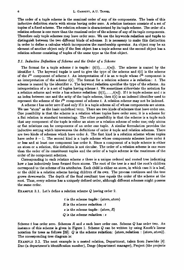
EXAMPLE 3.1. Let's define a relation scheme Q having order 2.

t is the scheme t u p l e : (atom, atom) R is the scheme r e l a t i o n : t

s is the scheme t u p l e : (atom, R) Q is the scheme r e l a t i o n : s

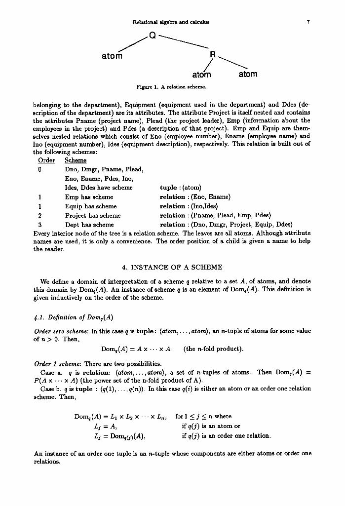
Scheme t has order zero. Schemes R and s each have order one. Scheme Q has order two. An instance of this scheme is given in Figure 1. Scheme Q can be written by using Knuth 's linear notation for trees as follows [29]: Q is the scheme re la t ion : (atom, r e l a t i o n : (atom, atom)). The corresponding tree diagram is:

EXAMPLE 3.2. The next example is a nested relation, Department, taken from Jaeschke [4]. Dno (a department 's identification number), Dmgr (department manager), Project (the projects

Relational algebra and calculus

R atom /

atom atom Figure 1. A relation scheme.

belonging to the department), Equipment (equipment used in the department) and Ddes (description of the department) are its attributes. The attribute Project is itself nested and contains the attributes Pname (project name), Plead (the project leader), Emp (information about the employees in the project) and Pdes (a description of that project). Emp and Equip are themselves nested relations which consist of Eno (employee number), Ename (employee name) and Ino (equipment number), Ides (equipment description), respectively. This relation is built out of the following schemes:

Order Scheme

0 Dno, Dmgr, Pname, Plead,

Eno, Ename, Pdes, Ino, Ides, Ddes have scheme

1 Emp has scheme

1 Equip has scheme

2 Project has scheme

3 Dept has scheme Every interior node of the tree is a relation scheme. The leaves are all atoms. Although attribute names are used, it is only a convenience. The order position of a child is given a name to help the reader.

t u p l e : (atom)

re la t ion : (Eno, Ename)

re la t ion : (Ino,Ides)

re la t ion : (Pname, Plead, Emp, Pdes)

re la t ion : (Dno, Dmgr, Project, Equip, Ddes)

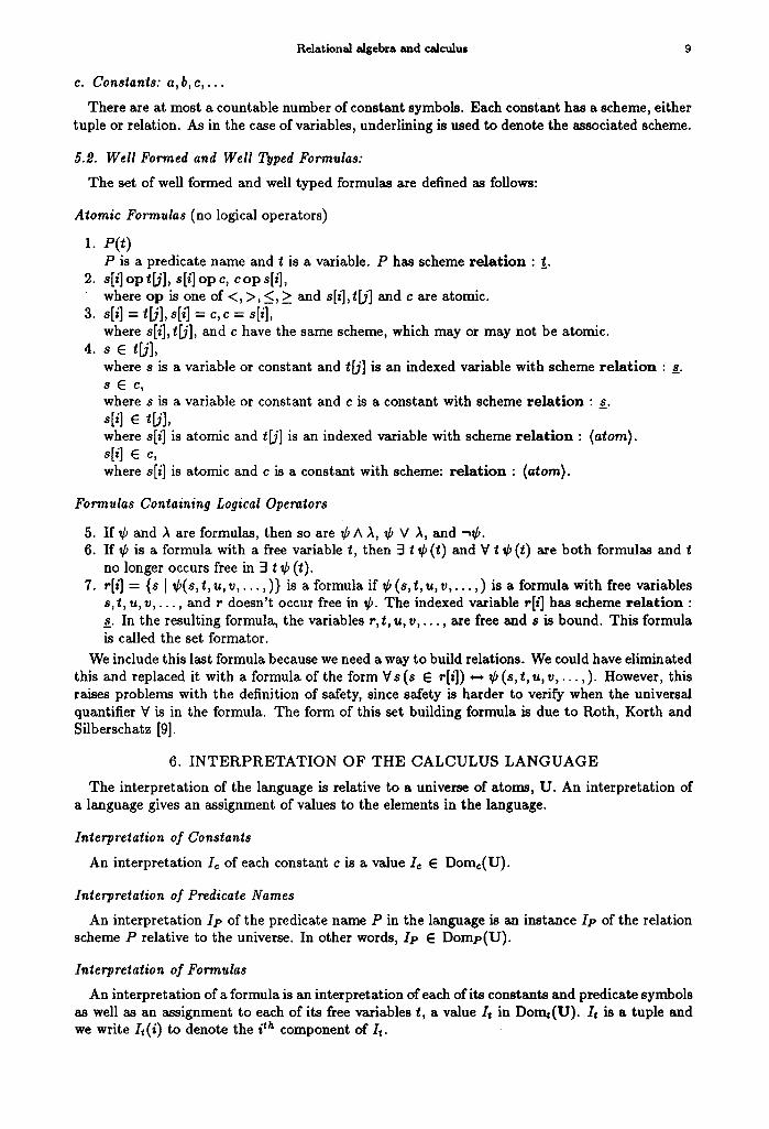
4. INSTANCE OF A SCHEME

We define a domain of interpretation of a scheme q relative to a set A, of atoms, and denote this domain by Domq(A). An instance of scheme q is an element of Domq(A). This definition is given inductively on the order of the scheme.

4.1. Definition of Domq(A)

Order zero scheme: In this case q is tup le : (a tom, . . . , atom), an n-tuple of atoms for some value of n > O. Then,

Domq(A) = A × . . . × A (the n-fold product).

Order I scheme: There are two possibilities. Case a. q is relat ion: (a tom, . . . , atom), a set of n-tuples of atoms. Then Domq(A) =

P(A x . . . x A) (the power set of the n-fold product of A). Case b. q is tup le : (q(1),. . . , q(n)). In this case q(i) is either an atom or an order one relation

scheme. Then,

Domq(A) = Lt × L2 x --. x Ln,

Li=A, Lj = Dom~(.i)(A),

for 1 _< j _< n where

if q(j) is an atom or

if q(j) is an order one relation.

An instance of an order one tuple is an n-tuple whose components are either atoms or order one relations.


Order k+l scheme: Again there are two possibilities. Case a . q is r e l a t i o n : t, where t is a tuple scheme of order k. Then,

Domq(A) = P(Domt(A)) .

An instance of an order k + 1 relation is a set of tuples of order k. Case b. q is t u p l e : (q (1 ) , . . . , q(n)). Each q(i) is either an a tom or an order k relation. Then

Domq(A) = L1 x L9 x . . . x Ln,

L# =A, L i = Domqc/)(A ),

for 1 < i < n where

if q(j) is an a tom or

if q(j) is a relation.

An instance of an order k + 1 tuple is an n-tuple whose components are either a toms or relation instances of order k + 1 or less, with at least one of the components having order k + 1.

4.2. Definition of Instance

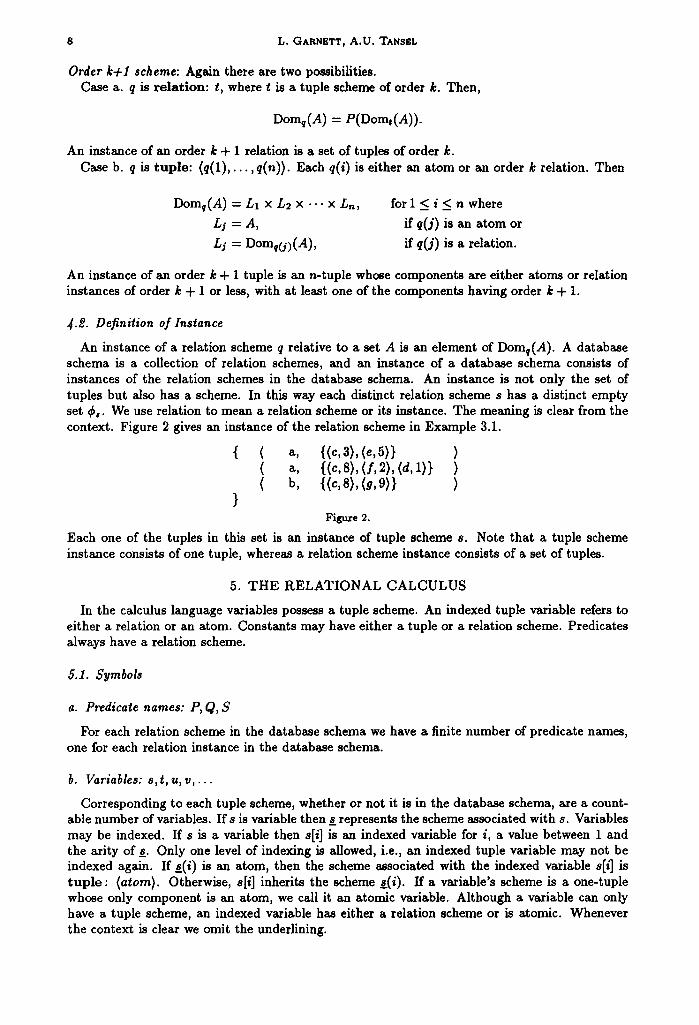
An instance of a relation scheme q relative to a set A is an element of Domq(A). A database schema is a collection of relation schemes, and an instance of a database schema consists of instances of the relation schemes in the database schema. An instance is not only the set of tuples but also has a scheme. In this way each distinct relation scheme s has a distinct empty set ¢0. We use relation to mean a relation scheme or its instance. The meaning is clear from the context. Figure 2 gives an instance of the relation scheme in Example 3.1.

{ ( a, {(c, 3), (e,5)} ) ( a, {(c,8),(f,2),(d,l)} ) ( b, {(c, 8), (g, 9)} )

Figure 2.

Each one of the tuples in this set is an instance of tuple scheme s. Note tha t a tuple scheme instance consists of one tuple, whereas a relation scheme instance consists of a set of tuples.

5. T H E R E L A T I O N A L C A L C U L U S

In the calculus language variables possess a tuple scheme. An indexed tuple variable refers to either a relation or an atom. Constants may have either a tuple or a relation scheme. Predicates always have a relation scheme.

5.1. Symbols

a. Predicate names: 19, Q, S

For each relation scheme in the database schema we have a finite number of predicate names, one for each relation instance in the database schema.

b. Variables: s , t , u, v, . . .

Corresponding to each tuple scheme, whether or not it is in the database schema, are a countable number of variables. I f s is variable then s_ represents the scheme associated with s. Variables may be indexed. If s is a variable then s[i] is an indexed variable for i, a value between 1 and the ari ty of _s. Only one level of indexing is allowed, i.e., an indexed tuple variable may not be indexed again. I f _s(i) is an a tom, then the scheme associated with the indexed variable s[i] is t u p l e : (atom). Otherwise, s[i] inherits the scheme s_.(i). I f a variable 's scheme is a one-tuple whose only component is an atom, we call it an atomic variable. Although a variable can only have a tuple scheme, an indexed variable has either a relation scheme or is atomic. Whenever the context is clear we omit the underlining.

Rdational algebra and calculus 9

e. Constants: a,b, c , . . .

There are at most a countable number of constant symbols. Each c°nstant has a scheme, either tuple or relation. As in the case of variables, underlining is used to denote the associated scheme.

5.~. Well Formed and Well Typed Formulas:

The set of well formed and well typed formulas are defined as follows:

Atomic Formulas (no logical operators)

1. P(t) P is a predicate name and t is a variable. P has scheme r e l a t i o n : t.

2. s[i]opt~], s[i]opc, cops[i], where op is one of <, > , < , > and s[i],t[j] and e are atomic.

3. s[i] = t[j], s[i] = c, e = sCi], where s[i],t~], and c have the same scheme, which may or may not be atomic.

4. s e t~], where s is a variable or constant and t[j] is an indexed variable with scheme r e l a t i o n : _s. 8 E e , where s is a variable or constant and c is a constant with scheme r e l a t i o n : _s. s[i] e t~], where s[i] is atomic and t[j] is an indexed variable with scheme r e l a t i o n : {atom). s[i] e c, where s[i] is atomic and c is a constant with scheme: r e l a t i o n : {atom}.

Formulas Containing Logical Operators

5. If ¢ and )~ are formulas, then so are ¢ A ~, ¢ V ~, and -~¢. 6. If ¢ is a formula with a free variable t, then 3 t ¢ (t) and V t ¢ (t) are both formulas and t

no longer occurs free in 3 t ¢ (t). 7. r[z] = {s I ¢(s , t, u, v , . . . , ) } is a formula if ¢ (s, t, u, v , . . . , ) is a formula with free variables

s,t , u , v , . . . , and r doesn't occur free in ¢. The indexed variable r[i] has scheme r e l a t i o n : _s. In the resulting formula, the variables r,t, u , v , . . . , are free and s is bound. This formula is called the set formator.

We include this last formula because we need a way to build relations. We could have eliminated this and replaced it with a formula of the form Vs (s G r[i]) ~ ¢ (s, t, u, v , . . . , ) . However, this raises problems with the definition of safety, since safety is harder to verify when the universal quantifier V is in the formula. The form of this set building formula is due to Roth, Korth and Silberschatz [9].

6. I N T E R P R E T A T I O N O F T H E C A L C U L U S L A N G U A G E

The interpretation of the language is relative to a universe of atoms, U. An interpretation of a language gives an assignment of values to the elements in the language.

Interpretation of Constants

An interpretation Ic of each constant c is a value Ic E Dome(U).

Interpretation of Predicate Names

An interpretation 1p of the predicate name P in the language is an instance Ip of the relation scheme P relative to the universe. In other words, Ip G Domp(U) .

Interpretation of Formnlas

An interpretation of a formula is an interpretation of each of its constants and predicate symbols as well as an assignment to each of its free variables t, a value It in Domt(U) . It is a tuple and we write It(i) to denote the i th component of It.

10 L. GARN~.TT, A.U. TANSEL

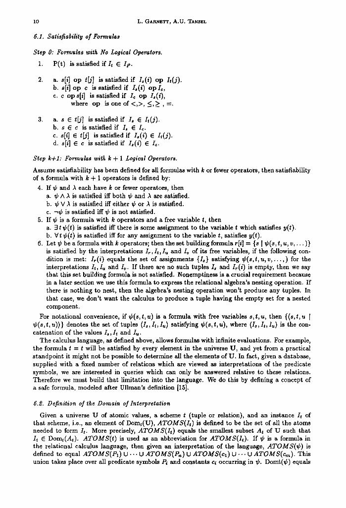
6.1. Satisfiability of Formulas

Step O: Formulas with No Logical Operators.

1. P(t) is satisfied if h • I~,.

. a. s[i] op t[j] is satisfied if Io(i) op h(j) . b. s[i] o p c is satisfied if I,(i) op lc , c. c ops[z] is satisfied if h o p Io(i),

where op is one of < ,> , _<,_> , =.

. a. s e t[j] is satisfied if h E h ( j ) . b. s E c is satisfied if I , E Ic. c. s[i] E t[j] is satisfied if I,(i) e It(j). d. s[i] e c is satisfied if Is(i) • Ic.

Step k÷l: Formulas with k + 1 Logical Operators.

Assume satisfiability has been defined for all formulas with k or fewer operators, then satisfiability of a formula with k + 1 operators is defined by:

4. If ¢ and ~ each have k or fewer operators, then a. ¢ A ~ is satisfied iff both ¢ and ~ are satisfied. b. ¢ V ,~ is satisfied iff either ¢ or ~ is satisfied. c. --¢ is satisfied iff ¢ is not satisfied.

5. If ¢ is a formula with k operators and a free variable t, then a. 3 t ¢(t) is satisfied iff there is some assignment to the variable t which satisfies y(t). b. Vt ¢(t) is satisfied iff for any assignment to the variable t, satisfies y(t).

6. Let ¢ be a formula with k operators; then the set building formula r[i] - {s [ ¢(s, t, u, v , . . . )} is satisfied by the interpretat ions/~, It, Iu and Iv of its free variables, if the following condition is met: It(i) equals the set of assignments {I,} satisfying ¢(s , t ,u ,v , . . . , ) for the interpretat ions/ t , Iu and Iv. If there are no such tuples Ia and It(i) is empty, then we say that this set building formula is not satisfied. Nonemptiness is a crucial requirement because in a later section we use this formula to express the relational algebra's nesting operation. If there is nothing to nest, then the algebra's nesting operation won't produce any tuples. In that case, we don't want the calculus to produce a tuple having the empty set for a nested component.

For notational convenience, if ¢(s, t, u) is a formula with free variables s, t, u, then {(s, t, u I ¢(s, t , u))} denotes the set of tuples (I0, It, I~) satisfying ¢(s, t ,u) , where (I,, It, 1,,) is the con- catenation of the values I,, It and I,,.

The calculus language, as defined above, allows formulas with infinite evaluations. For example, the formula t = t will be satisfied by every element in the universe U, and yet from a practical standpoint it might not be possible to determine all the elements of U. In fact, given a database, supplied with a fixed number of relations which are viewed as interpretations of the predicate symbols, we are interested in queries which can only be answered relative to these relations. Therefore we must build that limitation into the language. We do this by defining a concept of a safe formula, modeled after Ullman's definition [15].

6.2. Definition of the Domain of Interpretation

Given a universe U of atomic values, a scheme t (tuple or relation), and an instance It of that scheme, i.e., an element of Domt(U), ATOMS(I t ) is defined to be the set of all the atoms needed to form It. More precisely, ATOMS(I t ) equals the smallest subset At of U such that It E Domt(At). ATOMS( t ) is used as an abbreviation for ATOMS(I t ) . If ¢ is a formula in the relational calculus language, then given an interpretation of the language, ATOMS(C) is defined to equal ATOMS(P1) U ... U ATOMS(Pn) t3 ATOMS(e l ) U ... t3 ATOMS(cm). This union takes place over all predicate symbols P~ and constants cl occurring in ¢. Domt(¢) equals

Relational algebra and calculus 11

Domt(ATOMS(¢)) . This set contains all possible objects of scheme t built up from the atoms of predicates occurring in ¢. If the context is clear we let D~ denote Domt(¢).

The safety of formula ¢ with free variable t is defined relative to an interpretation of the predicate names and constant symbols in the formula. We define ¢ to be a safe formula when the following three conditions are satisfied:

1. {t I ¢(t)} is a subset of Domt(¢). This means that every interpretation of t satisfying ¢ is built out of the atoms occurring in the interpretation of the predicate names and constants occurring in ¢.

2. If 3u (w(u, v , . . . , )) is a subformula of ¢, then any interpretation of u which satisfies w is in Domu(w), no matter how the other free variables are interpreted.

3. IfVu (w(u, v , . . . , )) is a subformula of ~b, then any interpretation of u not in Don~ (w) satisfies w, no matter how the other free variables are interpreted.

This definition of safety is a direct extension of the one given by Ullman [15]. The next theorem gives a safe formula expressing the powerset.

THEOREM 6.1. Given any safe formula ~b(t) with one free variable, there is a safe formula w(s) with one free variable such that {s I w(s)} equals the powerset of{t [ ¢(t)}.

PROOF. Let ¢(t) be a safe formula with free variable t. Let w(s) be the formula 3 u (s(1) = u(1) A s(1) = {t [ t E u(1) A ¢(t)}). By definition, any variable in the calculus has a tuple scheme. However, we want the variable s to represent an element of the powerset. We do this by making s a tuple variable with one component. That component is a relation whose tuples have scheme t. For example, if t has scheme tuple : {atom,atom,atom) then s has scheme tuple : (relation: (atom,atom,atom)). The variable u has the same scheme as s and is needed in order to insure that to(s) is a safe formula. Although u ranges over all possible tuples in the universe, the rest of the formula places a limit on the possible values of u that can satisfy w and thus insuring the safety of w. It is easy to check that a 1-tuple satisfies w if and only if its unique component is a subset of tuples satisfying ¢. II

7. THE RELATIONAL ALGEBRA

The relational algebra is a collection of expressions. The operands of a relational algebra expression are either constant relations or variables representing a relation. The operations are union, intersection, difference, Cartesian product, projection, selection, nesting and unnesting. The standard derived operations such as intersection, join, division, etc., can be expressed in terms of these basic operations. A relational algebra expression is essentially a function. It accepts relations as arguments and outputs a computed relation. For notational convenience, if E is a relational algebra expression then EV(E) denotes the computed relation. We say that E expresses the relation EV(E) . Relation variables in algebra expressions correspond to predicate symbols in the calculus language.

7.1. Definition of the Algebraic Operations

E, R and S denote algebraic expressions.

1. Union: R U S. R and S have the same scheme. RUS has that scheme and E V ( R US) equals EV(R) UEV(S), the standard set union.

2. Intersection: R fl S. R and S have the same scheme. R NS has that scheme and E V ( R NS) equals EV(R)NEV(S) , the standard set intersection.

3. Set difference: R - S. R and S have the same scheme. R - S has that scheme and E V ( R - S ) equals E V ( R ) - E V ( S ) .

4. Cartesian product: E - R x S. R has scheme relation: ( , (1) , . . . , r(,)). S has scheme re la t ion : (s(1) , . . . , s(m)). E has scheme re la t ion : (e(1), . . . , e(n + m)), where e(i) = r(i) for 1 < i < n and e(i + n) = s(i) for 1 < i < m. EV(E) equals EV(R) x EV(S) , the standard set Cartesian product.


5. Projection: E -- ~ ( R ) . R has scheme r e l a t i o n : ( r ( 1 ) , . . . , r(n)) . Y = { Q , . . . ,ik} is a subset of the indexes {1 , . . . ,n}. E has scheme r e l a t i o n : (e (1) , . . . ,e(k)), where e(s) = r(i,) for 1 < s < k. E V ( E ) = { ( z l , . . . , z~) I 3 (Yl , . . . , Yn) E EV(R) and z , = Yi,, for 1 < s < k}, which can also be written as {t[Y] I t • EV(R)}.

6. Selection: E = aF(R). R has scheme r e l a t i o n : ( r ( 1 ) , . . . , r(n)). E has scheme r e l a t i o n : ( r ( 1 ) , . . . , r(n)).

F is a formula which selects tuples in the relation EV(R) to form the relation EV(E). In defining admissible formulas we could be very generous and permit many formulas, instead we keep our formulas simple. However, we show that more complicated selection formulas can be derived from the simple ones.

The format of F is i o p j where op is one of the elementary comparison operators: =, <, >, ¢ , <, ~. The operands i and j can either be an index to a tuple component in the relation or constant value. We use an apostrophe to distinguish a constant value from an index. The schemes for i and j must be the same. Furthermore, if o p is neither = nor ¢ , then r(i) and r(j) must both be atoms. If we view R as a tree structure, then i and j are either constants or refer to the children of the root since we only allow indexing on one level.

From this restricted class of formulas we can derive a much larger class. In what follows k, k l , . . . ,k, and h are constants or indexes to columns of the relation; that is they represent children of the root of the relation R. The following are the derived selection formulas:

6a. k E h . rk has scheme t u p l e : (atom), and rh has scheme r e l a t i o n : (atom).

65. ( k l , . . . , k , ) E h. h has scheme r e l a t i o n : ( r ( k l ) , . . . , r(k0)).

6c. h D k . h and k have the same relation scheme.

The second case permits grouping of constants or columns of the relation and treating this group as a tuple, to ask if that tuple is a member of a relation occurring either as a constant relation, or as another column of the original relation. The third case asks if the component relation in column k is a subset of the component relation in column h. The proof of these derived operations is deferred to the end of the definition. See Lemma 7.3.

EXAMPLE 7.1. R is a scheme consisting of 2-tuples. Each column of the 2-tuple is a set of atoms. R - r e l a t i o n : ( r e l a t i o n : atom, r e l a t i o n : atom). An instance of R is:

( (a,c,d}, (a,b,c,d} ) ( (b,c,d}, (a,b} ) ( {e, f ,g}, ( e , f , h , d ) ) ( {a,c,d}, {a,c,d} )

If F is the formula tbl E 1 then aF(R) produces:

{ ( {b,c,d}, (a,b} )

}

If F is the formula 2 _D 1 then o'F(R ) produces:


{ ( {a,c,d}, {a,b,c,d} ) ( {a,c,d}, {a,c,d} )

}

Selection formulas with logical connectives can be derived from this simple selection format. The conjunction of two formulas is the consecutive application of selection by the formulas. The disjunction of two formulas is the union of their selection. Negation of a formula is handled by pushing the negation into the atomic components of the formula and noting that the negation of any op is also an op . We are also able to derive an operation that performs selection using the membership operator on deeply nested structures. See Lemma "/.4 at the end of this section.

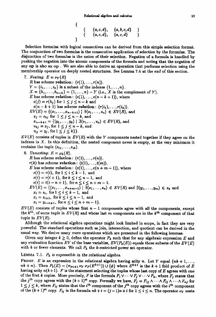
7. Nesting: E = ts,(R) R has scheme re la t ion: ( r (1) , . . . , r(n)). Y = {ia, . . . ,ik} is a subset of the indexes {1, . . . ,n}. X = {hx, . . . , ha-k} -- {1, . . . , n} - Y (i.e., X is the complement of Y). g has scheme re la t ion : (e(1) , . . . , e(n - k + 1)), where

e(j) = r(hj) for l _ < j _ < n - k a n d e ( n - k + 1) has scheme re la t ion: (r( i , ) , . . . ,r(ik)).

EV(E) = { ( z , , . . . , z , - ~ + l ) I 3 ( s l , . . . , s , ) E EV(R), and z j = s h j for l _ < j < n - k , and z , -k+ l = {(Yl,... ,Yk) [ 3(Vl,.. . ,v ,) 6 EV(R) , and v h j = z j , f o r l _ < j < n - k , and vir = yr, for 1 _< j _< k}) .

EV(E) consists of tuples in EV(R) with the Y components nested together if they agree on the indexes in X. In this definition, the nested component never is empty, at the very minimum it contains the tuple ( s i l , . . . , sik).

8. Unnesting: E = p~(R). R has scheme r e h t i o n : ( r (1) , . . . , r(n)). r(k) has scheme re la t ion: (t(1), . . . ,t(m)). g has scheme re la t ion : (e(1) , . . . , e(n + m - 1)), where

e(i) = r(i), for 1 < i < k - 1, and e ( i ) = r ( i + l ) , f o r k < i < n - 1 , and e( i) = t( i - n + l ), f o r n < i < n + m - 1 .

EV(E) = {(zl,...,zn+m-,)[ 3(st,...,s,) 6 EV(R) and 3(111,...,Vm) E s~ and z i = s l , f o r l < i < k - 1 , and xi = si+l, fork < i < n - 1, and zl = y i - ,+ l , f o r n < i < n + r n - 1 } .

EV(E) consists of tuples whose first n - 1 components agree with all the components, except the k th, of some tuple in EV(R) and whose last m components are in the k th component of that tuple in EV(R).

Although the relational algebra operations might look limited in scope, in fact they are very powerful. The standard operations such as join, intersection, and quotient can be derived in the usual way. We derive many more operations which are presented in the following lemmas.

Given any integer k > 0, define the operator Pk such that for any algebraic expression E and any evaluation function E V of the base variables, EV(Pk(E)) equals those subsets of the EV(E) with k or fewer elements. We call Pk the k-restricted power set operator.

LEMMA 7.1. Pk is expressible in the relational algebra.

PROOF. g is an expression in the relational algebra having arity n. Let Y equal {nk + 1 , . . . , nk + n}. Then Pk(E) = (~rk,+, zq, O'F(Ek+l)) O {~} where E k+* is the k + 1 fold product of E having arity n(k+ 1). F is the statement selecting the tuples whose last copy of E agrees with one of the first k copies. More precisely, F is the formula F, V. . . V Fj V. . . V Fk, where Fj states that the jth copy agrees with the (k + 1) "t copy. Formally we have, Fj = Fir A . . . A Fij A . . . A F, r for 1 _< j < k, where Fir states that the i th component of the jth copy agrees with the i th component of the (k + 1) *t copy. Fir is the formula nk + i = (j - 1)n + i for 1 < i < n. The operator ~q, nests


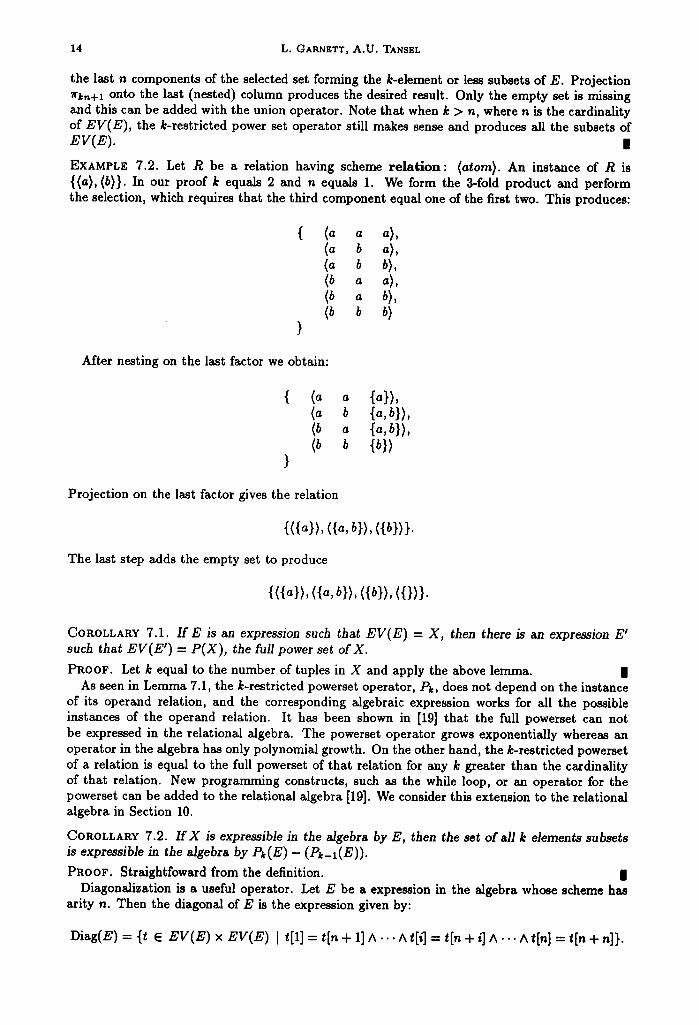
the last n components of the selected set forming the k-element or less subsets of E. Projection ~rk,+l onto the last (nested) column produces the desired result. Only the empty set is missing and this can be added with the union operator. Note that when k > n, where n is the cardinality of EV(E) , the k-restricted power set operator still makes sense and produces all the subsets of EV(E) . |

EXAMPLE 7.2. Let R be a relation having scheme relation: (atom). An instance of R is {(a), (b)}. In our proof k equals 2 and n equals 1. We form the 3-fold product and perform the selection, which requires that the third component equal one of the first two. This produces:

{ (a a a),

(~ b b), (b a a), (b a b), ~b b b)

}

After nesting on the last factor we obtain:

(~ ~ {~}), (a b {a,b}), <b a {a,b}), <b b {b})

Projection on the last factor gives the relation

{<{a}),<{a,b}),({b})}.

The last step adds the empty set to produce

{({a}), ({a, b}), ({b}), ({})}.

COROLLARY 7.1. I f E is an expression such that EV(E) = X , then there is an expression E' such that EV(E') = P(X), the fuji power set of X.

PROOF. Let k equal to the number of tuples in X and apply the above lemma. | As seen in Lemma 7.1, the k-restricted powerset operator, P~, does not depend on the instance

of its operand relation, and the corresponding algebraic expression works for all the possible instances of the operand relation. It has been shown in [19] that the full powerset can not be expressed in the relational algebra. The powerset operator grows exponentially whereas an operator in the algebra has only polynomial growth. On the other hand, the k-restricted powerset of a relation is equal to the full powerset of that relation for any k greater than the cardinality of that relation. New programming constructs, such as the while loop, or an operator for the powerset can be added to the relational algebra [19]. We consider this extension to the relational algebra in Section 10.

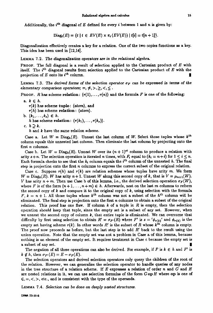
COROLLARY 7.2. If X is expressible in the a/gebra by E, then the set of all k elements subsets is expressible in the algebra by Pk(E) - (Pk-I(E)).

PROOF. Straightfoward from the definition. | Diagonalization is a useful operator. Let E be a expression in the algebra whose scheme has

arity n. Then the diagonal of E is the expression given by:

Diag(E) = {t • EV(E) x EV(E) I till = t[n + 1] A . . .A t [ s 1 = t in+s1 A. . .At [n ] = t in+n]} .

Relational algebra and calculus

Additionally, the ith diagonal of E defined for every i between 1 and n is given by:

15

Diag,(E) - {t I t e E V ( E ) x ~i (E V (E ) ) I t[il = t [ , + i l l

Diagonalization effectively creates a key for a relation. One of the two copies functions as a key. This idea has been used in [12,14].

LEMMA 7.2. The diagonalization operators are in the relational algebra.

PROOF. The full diagonal is a result of selection applied to the Cartesian product of E with itself. The /th diagonal results from selection applied to the Cartesian product of E with the projection of E onto its i th column, m

LEMMA 7.3. The derived forms of the selection operator trF can be expressed in terms of the elementary compar/son operators; --, ~ , >, >_, <, < .

PROOF. R has scheme r e l a t i o n : ( r ( 1 ) , . . . , r (n)) and the formula F is one of the following:

a. k E h . r(k) has scheme t u p l e : (atom), and r(h) has scheme r e l a t i o n : (atom).

b. (k l , . . . ,k0) e h. h has scheme r e l a t i o n : { r ( k l ) , . . . , r (~ , ) ) .

c. h D k . h and k have the same relation scheme.

Case a. Let W = Diagh(R). Unnest the last column of W. Select those tuples whose k th column equals this unheated last column. Then eliminate the last column by projecting onto the first n columns.

Case b. Let W = Diagh(R). Unnest W over its (n + 1) st column to produce a relation with arity s+n . The selection operation is i terated n times, with F~ equal to (k~ = n+i ) for 1 < i < n. Each formula checks to see that the hi column equals the ith column of the unnested h. The final step is projection onto the first n columns to express the correct subset of the original relation.

Case c. Suppose r(h) and r(k) are relation schemes whose tuples have arity m. We form W = Diagk(R). W has arity n + 1. Unnest W along this second copy of k, that is V = t tn+l(W). V has arity n + m. Then use Case b of this lemma, i.e., the derived selection operation ~rF(W), where F is of the form (n + 1 , . . . , n + m) E h. Afterwards, nest on the last m columns to reform the second copy of k and compare it to the original copy of k, using selection with the formula F , k = n + 1. All those tuples whose k th column was not a subset of the h th COIulTln will be eliminated. The final step is projection onto the first n columns to obtain a subset of the original relation. This proof has one flaw. If column k of a tuple in R is empty, then the selection operation should keep that tuple, since the empty set is a subset of any set. However, when we unnest the second copy of column k, that entire tuple is eliminated. We can overcome that difficulty by first using selection to obtain R' = ~F' (R) where F ' is s = '¢r(~)' and Cr(k) is the empty set having scheme r(k). In other words R I is the subset of R whose k th column is empty. The proof now proceeds as before, but the last step is to add R' back to the result using the union operation. Note that the empty set was not a problem in Case a of this lemma, because nothing is an element of the empty set. It requires t reatment in Case c because the empty set is a subset of any set. m

The negation of all these operations can also be derived. For example, if F is k 6 h and F ~ is k ~ h, then aF, (E) = E - o'F(E ).

The selection operators and derived selection operators only query the children of the root of the relation. However, we can generalize the selection operator to handle queries of any nodes in the tree structure of a relation scheme. If E expresses a relation of order n and G and H are nested relations in it, we can use selection formulas of the form G o p H where o p is one of E, =, <, >, etc., and is consistent with the type of the operands.

LEMMA 7.4. Selection can be done on deeply nested structures.

23-10-B

16 L. OARNETT, A.U. TANSBL

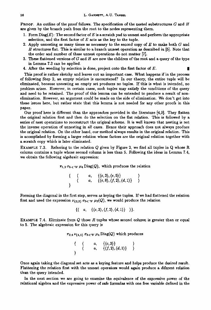
PROOF. An outline of the proof follows. The specification of the nested substructures G and H are given by the branch path from the root to the nodes representing them.

1. Form Diag(E): The second factor of E is a scratch pad to unnest and perform the appropriate selection, and the first factor of E acts as the key to the tuph.

2. Apply unnesting as many times as necessary to the second copy of E to make both G and H structures flat. This is similar to a branch unnest operation as described in [5]. Note that the order and number of these unnest operations do not matter [7].

3. These flattened versions of G and H are now the children of the root and a query of the type in Lemma 7.3 can be applied.

4. After the weeding by selection is done, project onto the first factor of E. |

This proof is rather sketchy and leaves out an important case. What happens if in the process of following Step 2, an empty relation is encountered? In our theory, the entire tuple will be eliminated, because unnesting an empty set produces no tuples. If this is what is intended, no problem arises. However, in certain cases, such tuples may satisfy the conditions of the query and need to be retained. The proof of this lemma can be extended to produce a result of non- elimination. However, an argument could be made on the side of elimination. We don't get into these issues here, but rather state that this lemma is not needed for any other proofs in this paper.

Our proof here is different than the approaches provided in the literature [4,9]. They flatten the original relation first and then do the selection on the flat relation. This is followed by a series of nest operations to reconstruct the original scheme. It is well known that nesting is not the inverse operation of unnesting in all cases. Hence their approach does not always produce the original relation. On the other hand, our method always results in the original relation. This is acomplished by forming a larger relation whose factors are the original relation together with a scratch copy which is later eliminated.

EXAMPLE 7.3. Referring to the relation Q given by Figure 2, we find all tuples in Q whose tt column contains a tuple whose second column is less than 5. Following the ideas in Lemma 7.4, we obtain the following algebraic expression:

Irl,2 a5 < '5' #4 Diag(Q), which produces the relation

{ ( ) ( a, {(c, 8), (f, 2), (d, 1)} )

}

Forming the diagonal in the first step, serves as keying the tuples. If we had flattened the relation first and used the expression u{2,s} as< ,5, #2(Q), we would produce the relation

{( a, {(c ,3) , ( f , 2),(d, 1)} )}.

EXAMPLE 7.4. Eliminate from Q those R tuples whose second column is greater than or equal to 5. The algebraic expression for this query is

r3,4 V{4,5} 0"5<'5' 1-/4 Diag(Q) which produces

{ ( a, {(c, 3)} ) ( . , { ( f ,2) , (d, 1>} )

}

Once again taking the diagonal set acts as a keying feature and helps produce the desired result. Flattening the relation first with the unnest operators would again produce a diferent relation than the query intended.

In the next section we are going to examine the equivalence of the expressive power of the relational algebra and the expressive power of safe formulas with one free variable defined in the


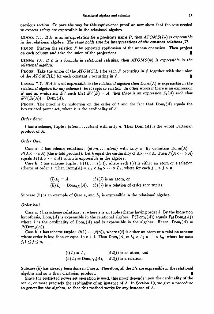
previous section. To pave the way for this equivalence proof we now show that the sets needed to express safety are expressible in the relational algebra.

LEMMA 7.5. I f Ip iS an interpretation for a predicate name P, then A T O M S ( I p ) is expressible in the relational algebra. The same holds true for interpretations of the constant relations [7].

PROOF. Flatten the relation P by repeated application of the unnest operation. Then project on each column and take the union of the projections. II

LEMMA 7.6. I f ¢ IS a formula in relational calculus, then A T O M S ( t ) IS expressible in the relational algebra.

PROOF. Take the union of the A T O M S ( I p ) for each P occurring in ¢ together with the union of the A T O M S ( I t ) for each constant c occurring in ¢. |

LEMMA 7.7. I rA is a set expressible in the relational algebra then Domt(A) is expressible in the relational a/gebra for any scheme t, be it tuple or relation. In other words i f there is an expression E and an evaluation E V such that E V ( E ) = A, then there is an expression Et(A) such that EV(E t (A ) ) = Domt(A).

PROOF. The proof is by induction on the order of t and the fact that Dome(A) equals the k-restricted power set, where k is the cardinality of A.

Order Zero:

t has a scheme, t u p l e : product of A.

(a tom, . . . , atom) with arity n. Then Domt(A) is the n-fold Cartesian

Order One:

Case a: t has scheme r e l a t i o n : (a tom, . . . ,a tom) with arity n. By definition Dome(A) = P(A x . . . x A) (the n-fold product). Let k equal the cardinality of A x--- x A. Then P(A x . . . × A) equals Pk(A x ... x A) which is expressible in the algebra.

Case b: t has scheme t u p l e : ( t (1) , . . . , t(n)), where each t(i) is either an atom or a relation scheme of order 1. Then Domt(A) = L1 × L2 x . . . × Ln, where for each j , 1 < j < n,

(i) Lj = A, if t ( j ) is an atom, or

(ii) Lj = Domt(j)(A), if t ( j ) is a relation of order zero tuples.

Subcase (ii) is an example of Case a, and Lj is expressible in the relational algebra.

Order k-I-I:

Case a: t has scheme r e l a t i on : s, where s is an tuple scheme having order k. By the induction hypothesis, Dom,(A) is expressible in the relational algebra. P(Dom,(A)) equals Pk(Dom,(A)) where k is the cardinality of Doms(A) and is expressible in the algebra. Hence, Domt(A) = P(Dom,(A)) .

Case b: t has scheme t u p l e : ( t (1) , . . . , t(n)), where t(i) is either an atom or a relation scheme whose order is less than or equal to k + 1. Then Dom:(A) = L1 × L2 × .-- × Ln, where for each j , l < j < _ n ,

(i) Lj = A, if t ( j ) is an atom, and

(ii) Lj = Domt(j)(A), if t( j) is a relation.

Subcase (ii) has already been done in Case a. Therefore, all the L's are expressible in the relational algebra and so is their Cartesian product. |

Since the restricted power set operation is used, this proof depends upon the cardinality of the set A, or more precisely the cardinality of an instance of A. In Section 10, we give a procedure to generalize the algebra, so that this method works for any instance of A.

18 L. GARNETT, A.U. T^NSEL

LEMMA 7.8. Given a formula ¢ having any number of free variables, a tuple scheme t, and an interpretation I of the predicate symbols occurring in 42, then Dora,(42), as defined in section 5, is expressible in the relational algebra. /n other words, there is an algebraic expression E¢,t,I such that EV(E¢,t,I) = Domt(42).

PROOF. Domt(42) = Domt(ATOMS(42)). Let A = A T O M S ( C ) and apply Lemma 7.7. Once the interpretation of the base relations is fixed, we can determine the cardinality of the set of the atoms occurring in relations used in 42. The restricted powerset operator accomplishes the desired result. |

EXAMPLE 7.5. A safe formula expressing the query in example 7.4 is 3s(Q(s) A t[1] - s[1] A t[2] = {u [ u E s[2] A u[2] < 5}). In order to translate this formula into a relational algebra expression, we need to construct relational algebra expressions for ATOMS(42), Domt(42), Dom,(42), and Domu(42). ATOMS(42) - 7rl(Q) u ~r2/J2(Q) u lra/~2(Q) which equals {a ,b , e ,d , e , f , g , l , 2 ,3 ,5 ,8 ,9} . The variable u has scheme t u p l e : (atom, atom). Domu(42) equals ATOMS(42) x ATOMS(42). The variables s and t have scheme t u p l e : (atom, r e l a t i o n : (atom, atom)) and hence, Dom,(42) equals Dome(42). Both are equivalent to ATOMS(42) x P ( A T O M S ( ¢ ) x ATOMS(C)) .

8. E Q U I V A L E N C E OF C A L C U L U S AND A L G E B R A

There are two ways of computing new relations from old ones. One uses relational algebra expressions and the other uses safe calculus formulas having one free variable. The formulation of an equivalence theorem must be done with care. The calculus can express the full powerset with a single formula which is independent of the relation. It is impossible to do this in the algebra. However, given an interpretation of the base relations, there is a single algebraic expression which results in the powerset of the input relation. The expression for the powerset operator depends upon the cardinality of the evaluation of the constant relations and variable relations occurring in the expression representing the input relation. We prove the equivalence theorem in two steps: Theorem 8.1 translates algebra expressions into calculus formulas, and Theorem 8.2 translates from the calculus to the algebra.

THEOREM 8.1. Given any expression E in the relational algebra, there is a safe formula ¢13 in the calculus such that for any evaluation E V of the relation variables and constant relations, the set o f t satisfying CE expresses the same relation. That is, {t [ CE(t)} = EV( E).

PROOF. The proof is by induction on the number of operators in E.

Part L Basis: E Has No Operators:

Case a: E expresses a constant relation. We use induction on the order of the scheme of E.

Order 1:

The scheme of E is r e l a t i o n : (a tom, . . . ,a tom) with arity n. Suppose E represents the set { t l , . . . ,tin}. Let Ei represent the set consisting of the tuple ti. Then EV(Ei) equals t I ¢i(t) where ¢i(t) is the formula (t[1] = ti[1] A . . . A tin] = ti[n]). It is easy to see that ¢i is a safe formula. Since E is a union of the Ei where i varies from 1 to m, we can conclude that E and the safe formula, ¢1(t) V- . - V era(t), represent the same set.

Order k+l:

The scheme of E is r e l a t i o n : (e(1) , . . . , e(n)). Each e(i) is either an atom or a relation scheme of order k or less. Suppose the set represented by E consists of m tuples { t l , . . . ,tin} of arity n. Let El be the expression representing {ti}, then as before E is equivalent to E1 U . . . U Era. The components of each ti are either atoms or relations of order k or less. By the induction hypothesis, any constant relation expressing a relation of order k or less can be expressed by a safe calculus expression. Hence, given any i between 1 and m, and any j between 1 and n, if e(j) is a relation scheme, then there is a safe formula ¢i,j(t) such that ti~] equals {s [ ¢ i j ( s )} . If e[j] is not a relation, then the translation is even simpler, namely t~[j] equals cid where cij , is an atomic


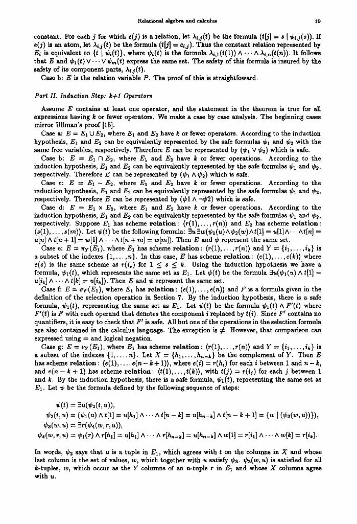
constant. For each j for which e(j) is a relation, let ~i,j(t) be the formula (t[j] = s I ¢ , j ( s ) ) . If e(j) is an atom, let ~iz(t) be the formula (t[j] = c~j). Thus the constant relation represented by Ei is equivalent to {t [ el(t)}, where ¢i(t) is the formula ,~i,l(t(1)) A . . . ^ )q,n(t(n)). It follows that E and ~)l(t) V " " V Crn(t) express the same set. The safety of this formula is insured by the safety of its component parts, ~ij(t) .

Case b: E is the relation variable P. The proof of this is straightfoward.

Part H. Induction Step: k-t-1 Operators

Assume E contains at least one operator, and the statement in the theorem is true for all expressions having k or fewer operators. We make a case by case analysis. The beginning cases mirror Ullman's proof [15].

Case a: E = Ex U E2, where EI and E2 have k or fewer operators. According to the induction hypothesis, Ex and E2 can be equivalently represented by the safe formulas Cx and ¢~ with the same free variables, respectively. Therefore E can be represented by (¢x V ¢2) which is safe.

Case b: E = E1 fq E2, where Ex and E2 have k or fewer operations. According to the induction hypothesis, E1 and E2 can be equivalently respectively. Therefore E can be represented by (¢x

Case c: E = E x - E 2 , where Ex and E2 have induction hypothesis, E1 and E~ can be equivalently respectively. Therefore E can be represented by (¢1

Case d: E = Ex x E2, where Ex and E2 have

represented by the safe formulas ¢1 and ¢2, ^ ¢2) which is safe. k or fewer operations. According to the

represented by the safe formulas ¢1 and ¢2, ^-~¢2) which is safe. k or fewer operations. According to the

induction hypothesis, E1 and E2 can be equivalently represented by the safe formulas ¢1 and ¢2, respectively. Suppose E1 has scheme re la t ion: ( r (1) , . . . , r (n) ) and E2 has scheme re la t ion: (s(1), . . . , s(m)). Let ¢(t) be the following formula: 3u 3w(¢1 (u)A ¢2(w) At[l] = u[1] A.. . At [n] = u[n] A t[n + 1] = w[1] A . . . A t[n + m] = w[m]). Then E and ¢ represent the same set.

Case e: E = ~rv(Ex), where Ex has scheme re la t ion: (r(1), . . . ,r(n)) and Y = {ix,. . . ,i~} is a subset of the indexes {1, . . . , n}. In this case, E has scheme re la t ion : (e(1) , . . . , e(k)) where e(s) is the same scheme as r(i,) for 1 < s < k. Using the induction hypothesis we have a formula, Ca(t), which represents the same set as Ex. Let ¢(t) be the formula 3u(¢l(u) ^ t[1] = u[ix] ^ . . . A t[k] = u[i~]). Then E and ¢ represent the same set.

Case f: E = aF(Ex), where Ex has re la t ion: (e(1) , . . . , e(n)) and F is a formula given in the definition of the selection operation in Section 7. By the induction hypothesis, there is a safe formula, Cx(t), representing the same set as Ex. Let ¢(t) be the formula ¢l( t) ^ F'(t) where F~(t) is F with each operand that denotes the component i replaced by t(i). Since F ~ contains no quantifiers, it is easy to check that F ~ is safe. All but one of the operations in the selection formula are also contained in the calculus language. The exception is 5. However, that comparison can expressed using = and logical negation.

Case g: E -- zsr(E1), where Ex has scheme re la t ion: (r(1), . . . ,r(n)) and r = {ix,. . . ,i~} is a subset of the indexes {1,. . . ,n}. Let X = {ha,. . . ,hn-k} be the complement of Y. Then E has scheme re la t ion: (e(1) , . . . , e(n - k + 1)), where e(i) = r(hi) for each i between 1 and n - k, and e(n - k + 1) has scheme re la t ion: (t(1), . . . ,t(k)), with t( j) = r(ij) for each j between 1 and k. By the induction hypothesis, there is a safe formula, ¢1(t), representing the same set as El. Let ¢ be the formula defined by the following sequence of steps:

¢ ( t ) = au(,/,=(t, u)) , ¢2(t , u) = (¢1(~,) A t[1] = u[h~] A . - . A t[n - ~] = u[h ,_k] ^ t in -- k + 1] = {to I ( ¢ 3 ( " , u ) ) } ) ,

¢~(,,,, u) = 3, ' (¢,~(~, r, u)),

¢,(,.,,, r, u) = ¢~(, ' ) A ,'[h~] = u[h~] A . . . A , ' [h , -k ] = u[h,_, , ] A ~[1] = ,-Jill A . . . ^ ,.,@] = , % ] .

In words, ¢2 says that u is a tuple in El, which agrees with t on the columns in X and whose last column is the set of values, w, which together with u satisfy Ca. Cs(w, u) is satisfied for all k-tuples, w, which occur as the Y columns of an n-tuple r in E1 and whose X columns agree with u.


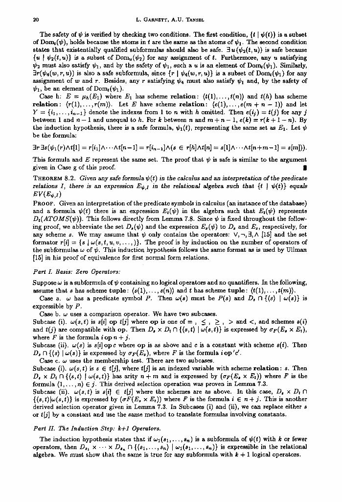
The safety of 4 is verified by checking two conditions. The first condition, {t [ 4(t)} is a subset of Dora,(4), holds because the atoms in t are the same as the atoms of 41. The second condition states that existentially qualified subformulas should also be safe. 3 u (42(t, u)) is safe because {u I 42(t, u)} is a subset of Domu(42) for any assignment of t. Furthermore, any u satisfying 42 must also satisfy 41, and by the safety of 41, such a u is an element of Dome(41). Similarly, 3r(44(w, r, u)) is also a safe subformula, since {r ] 44(w, r, u)} is a subset of Domt(41) for any assignment of w and r. Besides, any r satisfying 44 must also satisfy 41 and, by the safety of 41, be an element of Dom,(41).

Case h: g = /~h(El) where El has scheme relation: (t(1),...,t(n)) and t(h) has scheme relation: (r(1),...,r(m)). Let E have scheme relation: (e(1),...,c(m + n- 1)) and let Y = { i l , . . . , i n - l ) denote the indexes from 1 to n with h omitted. Then e(ij) = t(j) for any j between 1 and n - 1 and unequal to h. For k between n and m + n - 1, e(k) = r(k + 1 - n). By the induction hypothesis, there is a safe formula, 41(t), representing the same set as El . Let 4 be the formula:

3r3s(41(r)At[1] = r [ i l ] A . . . A t [ n - l ] = r[in-x]A(s E r[h]At[n] = s[1]A.. .At[n+m--1] = s[m])).

This formula and E represent the same set. The proof that 4 is safe is similar to the argument given in Case g of this proof. |

THEOREM 8.2. Given any safe formula 4(t) in the calculus and an interpretation of the predicate relations I, there is an expression E~,I in the relationM algebra such that {t [ 4(t)) equMs EV(E¢,I) PROOF. Given an interpretation of the predicate symbols in calculus (an instance of the database) and a formula 4(t) there is an expression E~(4) in the algebra such that Et (4) represents Dr(ATOMS(4)) . This follows directly from Lemma 7.8. Since 4 is fixed throughout the following proof, we abbreviate the set D, (4) and the expression E , (4 ) to D, and E~, respectively, for any scheme s. We may assume that 4 only contains the operators: V,-~, 3, A [15] and the set formator r[i]= {s [co(s,t, u, v , . . . , ) } . The proof is by induction on the number of operators of the subformulas w of 4. This induction hypothesis follows the same format as is used by Ullman [15] in his proof of equivalence for first normal form relations.

Part L Basis: Zero Operators:

Suppose co is a subformula of 4 containing no logical operators and no quantifiers. In the following, assume that s has scheme t u p l e : ( s (1) , . . . , s(n)) and t has scheme t u p l e : ( t (1) , . . . , t(m)).

Case a. co has a predicate symbol P. Then co(a) must be P(s) and Do N {(s) ] co(a)} is expressible by P.

Case b. co uses a comparison operator. We have two subcases. Subcase (i). co(a, t) is s[i] op t[j] where op is one of = , _< , >_ , > and <, and schemes s(i) and t(j) are compatible with op. Then D, x D, [7 {(s,t) I co(s,t)} is expressed by or(E0 x St), where F is the formula i o p n + j . Subcase (ii). co(a)is s[i] o p e where op is as above and c is a constant with scheme s(i). Then D, n {(s) [co(s)) is expressed by ~rF(E,), where F is the formula i o p ' d .

Case c. co uses the membership test. There are two subcases. Subcase (i). co(s, t) is s E t[j], where t[j] is an indexed variable with scheme r e l a t i o n : s. Then D, x D, N {(s,t) [ co(s,t)) has arity n + m and is expressed by (~F(E, x St)) where F is the formula ( 1 , . . . , n) E j . This derived selection operation was proven in Lemma 7.3. Subcase (ii). w(s, t) is s[i] E t[j] where the schemes are as above. In this case, D, x Dt f3 {(s,t)[co(s,t)) is expressed by (~F(Eo x St)) where F is the formula i ~ n + j . This is another derived selection operator given in Lemma 7.3. In Subcases (i) and (ii), we can replace either s or t[j] by a constant and use the same method to translate formulas involving constants.

Part IL The Induction Step: k-l-1 Operators.

The induction hypothesis states that if col(S: , . . . , s , ) is a subformula of 4(t) with h or fewer operators, then Dal x -. . x Da, f7 { ( s l , . . . , an) I col(sx, . . . , s , ) ) is expressible in the relational algebra. We must show that the same is true for any subformula with k -t- 1 logical operators.


Case a. W(yl , . . . ,yn) is Wl(Sl, . . . ,8h) Vtd2(z1,. . . ,zv) where {gl and w2 each have k or fewer operators. Set Y = {Yl,...,Y,~} equal to the free variables o fT , S = {s l , . . . , sh} equal to the free variables of Wl, and X = ( z l , . . . , z~} equal to the free variables of w~. Y equals the union of S and X, but S and X need not be disjoint. By the induction hypothesis there are algebraic expressions E~ and E~ representing

D,, x . . . x D,~ n {(Sl , . . . , sh) I tdl(Sl, . . . , 8h)}, and

Dx, x . . . x Dx. N { ( z l , . . . , z ~ ) I w2(Z l , . . . , z~ ) } , respectively.

Then, Dy~ x . . . x Dy. N{(y l , . . . , Yn) I W(Yl,-"", Yn)} is expressible as the union of two expressions W1 and W2, where W1 is E1 with a column D r added for each variable y occurring in Y but not in S, and likewise, W2 is E2 with a column D r added for each variable s occurring in Y but not in X. This construction can be found in Ullman's proof [15].

Case b. W(yl, . . . , yn ) is •1(81, ...,8h)^ W2(Zl,... ,Zv). Conjunction is handled exactly as disjunction except that the intersection of the two expressions W1 and W2 is formed, instead of their union.

Case c. W(Sl,. . . , an) is - ~ 1 ( s l , . . . , an), where Wl has k operators. By the induction hypothesis, there is an algebraic expression E1 representing D,, x . - . x D , . n {(Sl , . . . , an) [ Wl(Sl,... ,st,)}. Then, E,, x . . . x E , . - E1 is an algebraic expression for {(Sl, . . . , s , ) [ -~1(S l , . . . ,an)}.

Case d. w ( s l , . . . ,an) is 38n.bl(~gl(Sl,..., an-l-l)) where wl has k or fewer operators. Suppose scheme sl has cl columns. Then Dj~ x . . . x Dj.+~ has arity Cl + --. + cn+l and D~I x ..- x D , , has arity N = cl + . . . + cn. By the induction hypothesis, there is an algebraic expression E1 for Do~ x . . . x Do.+, N{(Sl , . . . , S,+l) [ w l ( s l , . . . , S,+l)}. Since Wl occurs in an existential subformula of the original safe formula w, w l ( S l , . . . , S,+l) can only be true if s ,+l is in D,.+I. Thus, we can conclude that ~'{1 ..... N}(E1) is an algebraic expression representing {(Sl, . . . ,sr , ) I W(Sl , . . . ,s ,~)}.

Case e. w ( s , t l , . . . , t n ) is (s[,l = {u ] Wl(U, t l , . . . , tn )} ) , where s has scheme tuple: ( s (1) , . . . , s (d) ) , u has scheme tup l e : (u (1 ) , . . . , u (m) ) , s[i] has scheme relat ion: (u(1) , . . . ,u(m)) , and wl has k operators. By the induction hypothesis, there is an algebraic expression E1 representing Du x D~I x . . . x Dtn N { ( u , t l , . . . , t n ) [ w l ( u , t l , . . . , t n ) } . Let us denote this last set by W. If the scheme for the tuple variable ti has cl columns, then W has arity n + c l + . . . + c n . Let Z equal Da x Dt~ x . . . x Dr, N~(S , t l , . . . ,tn) [w(s, t l , . . . ,tn)}, which also equals D, x D,, x . . . x D,~ N {(s, t l , . . . , t~,) [ s[i] = {u [Wl (U ,Q, . . . , t n ) } } . Z has arity d + cl + "'" + cn. Z can be represented by the following sequence of algebraic operations:

1. Nest W on the u columns, which in fact are the first m columns, W1 = v{1 ..... rn}(W)- W1 has arity 1 + cl + . . . + cn.

2. Add an s column using Cartesian product, W 2 = E , x W1. W 2 h a s a r i t y d + l + C l + " ' + c n .

3. Select those tuples in W2 whose i th column equals the nested u th column, W3 = aF(W2), where F is the formula i = d + 1.

4. We must get rid of the duplicated u th and ith columns, Z = lry(Ws), where Y are all the columns in W3 from 1 to d + 1 + Cl + . . . + cn excluding the (d + 1) st column which now duplicates the i th column. That is, Y = {1,2 , . . . , d, d + 2 , . . . , d + 1 + Cl + . . . + cn}. This produces the desired set, with the correct arity.

This completes the proof of Theorem 8.2. m

9. AN E X A M P L E

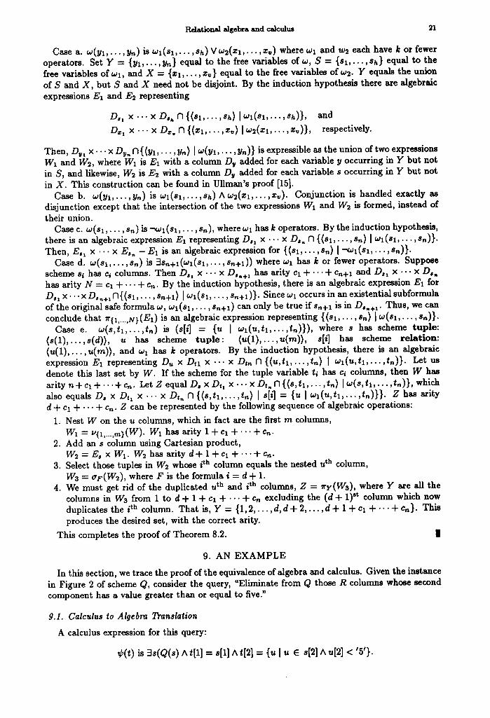
In this section, we trace the proof of the equivalence of algebra and calculus. Given the instance in Figure 2 of scheme Q, consider the query, "Eliminate from Q those R columns whose second component has a value greater than or equal to five."

9.1. Calculus to Algebra Translation

A calculus expression for this query:

¢(~) is 3s(Q(s) At[l] = s[1] At[2] = {u I u e s[2] ^ u[2] < ' 5 ' }

22 L. GARNETT, A.U. TANS~L

Example 7.5 gives the algebraic expressions Eu, Ea, Et for the domains Du, D, , and Dr. Tracing Theorem 8.2, we first translate subformulas o f ¢ having no logical operators, then all subformulas of ~b with one logical operator, and so on. Finally, the unique subformula with 5 logical operators, which is just ¢ itself, is translated.

Step 1: Subformulas with no logical operators:

a. u E s[2] is translated by ~le2(Eu x E, ) (Part I, Case c). b. u[2] < '5' is translated by ~2<,5,(E~) (Part I, Case b). c. t[1] = s[1] is translated by al=a(E~ × E, ) (part I case b). d. Q(s) is translated by Q (Part I, Case a).

Step 2: Subformulas with one logical operator:

a. u E s[2] A u[2] < '5' is translated by E1 = ale2(E~ x E,) fl (~2<,5, (Eu) × Ea) (Part II, Case d).

b. Q(s) A till = sill is translated by E2 = E~ × Qal=S (Et × E,) (Part 1I, Case d).

Step 3: There is one subformula with two logical operators. t[2] = {u I u E s[2] A u[2] < '5'} is translated by Es = 71"{1,3,4,5}(0"2=3 (E~ x I/{1,2}(E1))) (Part II, Case e).

In tracing this example, it is important to keep track of the arity of the schemes. The relation expressed by E1 has arity 4 since both Eu and Ea have arity 2. Hence, the first step ~{1,2}(E1) nests E1 on its first two columns which are in effect nesting on column u resulting in a scheme with arity 3. The next step adds a t column to create the relation Et × v{1,2}(E1) which has arity 5. Selection on 2 = 3, selects those tuples whose t[2] component equals the nested u column. The last step is a projection to get rid of column 2 which is now a duplicate of column 3.

Step 4: There is one subformulas with 4 logical operators. (There are no subformulas with 3 operators.) (Q(s) A t[1] = s[1]) ^ (t[2] = {u I u e s[2] A u[2] < '5'}) is translated by E2 N Es. Both E2 and E3 have schemes with arity 4. Thus, the resultant scheme has arity 4.

Step 5: There is one subformulas with 5 operators and that is ¢ itself. 3s(Q(s) A t[1] = s[1] A t[2] = {u l ues[2] A u[2] < '5 '}) is translated by lr{1,2}(E~ N Es) (Part II, Case d).

This completes the trace of Theorem 8.2. This is not an efficient algebraic expression, but it works. A more efficient algebraic expression for expressing this query is given in Example 7.5.

9.2. Algebra to Calculus Translation

Tracing Theorem 8.1, we translate the following algebra expression for the same query

It{s,4} z/{4,5} as<,6,p4Diag(Q).

Step 1. Diag(Q) is shorthand for aF(Q x Q), where F is the formula (1 = 3A2 = 4). Q x Q is translated to ¢0( t )where ¢0(t) is the formula 3u 3v(Q(u) A Q(v) At[l] - u[1] At[2] -- u[2] At[3] = v[1] A t[4] = v[2]) (Part II, Cased). Diag(Q) is translated to ¢1(t), where ¢1(t) is the formula ¢0(t) A till = t[3] A t[2] = t[4] (Part II, Case f).

Step 2. p4Diag(Q) is translated by ¢~(t), where ¢2(t) is the formula 3 r S S ( ¢ l ( r ) A t[1] = r[1] ^ t[2] -- r[2] A t[3] = r[3] ^ (s e r[4] ^ t[4] = s[1] ^ t[5] = s[2])) (Part II,Case h). Unnesting on the fourth column of Diag(Q) increased the arity by 1 since the fourth column was a relation containing 2-tuples. Hence t is a 5-tuple.

Step 3: as<,5, p4 Diag(Q) is translated by Ca(t), where Ca(t) is the formula ¢2( t )A t[5] < '5' (Part II, Case f).

Step 4: ~/{4,~} ~5<,5, p4 Diag(Q) is translated by ¢4(t), where ¢4(t) is the formula 3u(¢a(u) A t i l l = u[1] ^ t[2] = u[2] A t[3] = u[3] ^ t[4] = I 3 , ( ¢ s ( , ) ^ (r[Z] = u[1] ^ r[2] = u[2] ^ r[3] = u[3]) A (v[1] = r[4] A v[2] = r[5]))})(Part II, Case g).

Step 5:~r{a,4 } v{4,5} ¢5<,5' p4Diag(Q) is translated by ¢(t) , where ¢( t ) is the formula 3u(¢4(u)A t[1] = u[3] A t[2] = u[4]) (Part II, Case d).

This finishes the translation from algebra to calculus.


10. GENERALIZING THE EQUIVALENCE P R O O F

The relational calculus with the membership and set formator formulas can express the powerset of a relation. On the other hand, the relational algebra with nest and unnest operators can not express the powerset of a relation unless an instance for that relation is provided. Depending on the relation instance, a different algebra expression is generated for the powerset. So, this extended relational calculus is more powerful than the relational algebra with nest and unnest operators. We have shown that the relational calculus and algebra as defined in this work have the same expressive power provided an instance of the database is specified. This is the strongest possible equivalence assertion which can be proven. That is, any relational algebra expression can be translated to a relational calculus formula. But, a relational calculus formula cannot, in general, be translated to relational algebra unless a database instance is given.

We now show how to augment the relational algebra language so that it becomes as expressive as the relational calculus language for nested relations. There are several alternatives. One possibility consists of simply adding the power set operator to the relational algebra. A different approach consists of adding a while loop [19], an assignment operator and a comparison operator to the relational algebra with the nest and unnest operations. This algebra has the same expressive power as the relational calculus for nested relations. The following is an algorithm which creates the full power set for an algebra expression E.

Algorithm 1

begin k : = l Whi le Pk(E) # Pk+I(E) do

k:=k+l Endwhi le

e n d .

LI~MMA 10.1. Algorithm 1 calculates the power set of the relational algebra expression E.

PROOF. Algorithm 1 calculates PI(E),P2(E), . . . . Eventually it calculates Pn(E) where n is the cardinality of the relation created by E. Note that Pn(E) is the n th restricted power set operator which computes n or less subsets of EV(R). Algorithm 1 always halts. Since the relation instances in the database are finite, the while loop in Algorithm 1 is executed a finite number of times. For any k, k _< n, Pk(E) ~ P~+I(E) because Pk(E) contains subsets of E with k or fewer elements, whereas Pk+I(E) has subsets with k + 1 or fewer elements. On the other hand, when k reaches n, P~(E) mad Pk+I(E) contain the same subsets because the n or fewer and n + 1 or fewer subsets of EV(E) are the same, since E only contains a total of n tuples. |

THEOREM 10.1. Given any safe formula ¢(t) in the relational calculus, there is an equivalent expression E in the relational Mgebra, i.e., {t [ ¢(t)} - EV(E).

PROOF. Dom~(¢(t)) is expressible in the relational algebra. Use Algorithm 1 instead of the restricted power set operator Pk in Lemmas 7.7 and 7.8. The Dom,(¢(t)) will be generated independently of the interpretations of the symbols in ¢(t). The rest is the same as the proof of Theorem 8.2. |

Another alternative is adding a power set operator to the relational algebra. Such a relational algebra has the same expressive power as the relational calculus. The power set operator is used in Lemmas 7.7 and 7.8 to form Dom~(¢(t)). So, the translation from the relational calculus to the relational algebra will not be instance dependent. Theorem 6.1 gives the relational calculus expression for the power set operation of the relational algebra. This can be added as another case to the proof of Theorem 8.1. There is a subtle difference between the former and latter approaches. Algorithm 1 generates a different expression for each instance of E. However, the work is done within the algorithm and it is transparent in the calculus to algebra translation. On the other hand, adding the power set operator creates a fixed expression in the translation from calculus to algebra, which is independent of any particular instance. In either approach, translation from the algebra to the calculus always results in an expression which is instance independent.


11. CONCLUSION

In this paper, we define algebra and calculus languages for nested relations. A formal inductive definition is given, which is a generalization and refinement of previous definitions in the literature [3,7,9]. It is based on the tuple and relation distinction, and quantitatively assigns an order to a nested structure. The algebra and calculus languages we give are quite similar to the ones in the above mentioned studies.

We first show a limited equivalence between these languages since the translation (proof) from the calculus to the algebra requires an interpretation of the relations mentioned in the query expression. This is the strongest equivalence proof possible for relational algebra and calculus for nested relations. We later add more power to the relational algebra by augmenting it with programming constructs and provide an algorithm to construct the full power set of a relation independent of its instance. Then, we show that this augmented relational algebra has the same expressive power as the relational calculus; this equivalence does not depend upon the interpretations of the symbols mentioned in the algebra and calculus expressions.

REFERENCES

1. E. Codd, A relational model for large shared data banks, Comm,~nications of the ACM 13 (6), 377-387 (1970).

2. A. Makinouchi, A consideration on normal form of not-necessarily-normalized relation in the relational data model, Proceedings of the Third International Conference on VLDB, pp. 447--453, (1977).

3. G. Jaeschke and H. Schek, Remarks on the algebra of non-first normal form relations, Proceedings of the A CM SIGA CT-SIGMOD Symposium on Principles of Database Systems, pp. 124-138, (1982).

4. G. Jaeschke, Recursive algebra for relations with relation valued attributes, Technical Report, IBM Heidel- berg Scientific Center, (1984).

5. G. Jaeschke, Nonrecursive algebra for relations with relation valued attributes, Technical l~port, IBM Heidelberg Scientific Center, (1984).

6. H.-J. Schek and M. Scholl, An algebra for the relational model with relation-valued attributes, Information S~steme 11 (2) (1988).

7. P. Fischer and S. Thomas, Operators for non-first normal form relations, Proceedings of the 7th International Computer Software Applications Conference, (1983).

8. G. Kuper and M. Vardi, A new approach to database logic, Proceedings of the ACM SIGACT-SIGMOD S~mpoeium on Principles of Database Systems, pp. 86--96, (1984).

9. M. Roth, H. Korth and A. Silberschatz, Extended algebra and calculus for -~INF relational databases, ACM Transactions on Database Systems 13 (4), 389-417 (1988).

10. B. J,~cobs, Applied Database Logic, Prentice-Hall, (1985). 11. A.U. Tansel and L. Garnett, On Roth, Korth, Silberschatz's extended algebra and calculus for nested

relational databases, A CM Transactions on Database Systems (1992) (to appear). 12. G. Ozsoyogiu and M. Ozsoyogiu, An extmmion of relational algebra for emmnax7 tables, Proceedings of the

Second International Conference on Statistical Database Management, pp. 202-211, (1983). 13. G. Ozsoyogiu, M. Ozsoyoglu and V. Matos, Extending relational algebra and relational calculus with

set-valued attributes and aggregate functions, ACM TODS 12 (4), 566--592 (1987). 14. A. Klug, Equivalence of relationed algebra and relational calculus query languages having aggregate functions,

Journal of the ACM 29 (3), 899--717 (1982). 15. J.D. Uilman, Principles of Database Systems, Computer Science Press, (1982). 18. A.U. Aho and J.D. Ullman, Universality of data retrieval languages, Proc. of 6th POPL, pp. 110-117, San

Antonio, (1979). 17. A.K. Chandra and D. Harel, Computable queries for relational data bases, Journal of Computer and Systems

Science 21 (2), 156-178 (1980). 18. A.K. Chandra and D. Harel, Structure and complexity of relational queries, Journal of Computer and

Systems Science 25 (1), 99-128 (1985). 19. M. Gysenns and D. Van Gucht, The powerset algebra as a result of adding progrmmnJng constructs to the

nested relational algebra, Proceedings of SIGMOD, pp. 225-232, (1988). 20. J. Paredaens and D. Van Gucht, Possibilities and ]imitations of using fiat operators in nested algebra

expressions, Proceedings of the A CM SIGA CT-SIGMOD SlmpoJium on Principles of Database Systems, pp. 29-38, (1988).

21. D. Van Gucht, On the expressive power of relational edgehra for the unnormalized relational model, Proceed- ings of the ACM SIGACT-SlGMOD S{imposi,Lm on Principles of Database SyJtems, pp. 302-312, (1987).

22. S. Abiteboul and N. Bidoit, Non-first normal form relations to represent hierarchically organized data, Proceedings of the ACM SIGA CT-SIGMOD Symposium on Principles of Database Systems, pp. 191-200, (1984).


23. R. Hull and C.K. Yap, The format model: A theory of dAtsbue orsmization, Jo~raal o] the ACM 31 (3), 518-537 (1984).

24. M. Ozsoyoglu and L. Yuan, A new normal form for nested relations, ACM TODS 12 (1), 377-394 (1987). 25. M. Roth and H. Korth, The design of -~INF relational databases into nested normal form, Proceedings oJ

the AGM SIGMOD Con]., pp. 143--159, (1987). 26. Y. Kmlabayashi, K. Tanaka and K. Takeda, Synthesis of unnormalized relations incorporating more meaning,

Information Sclences 29 (2), 201-247 (1983). 27. P. Fischer and D. Van Gucht, Weak multivalued dependencies, Proceedings oJ ihe AGM SIGA CT-SIGMOD

Symposium on Principles of Database Systems, pp. 266-274, (1984). 28. D. Van Gucht and P. Fischer, Some classes of multilevel relational structures, Proceedings of the A CM

SIGA CT-SIGMOD S~mposi~m on Principles of Database Systems, pp. 60--69, (1986). 29. D.E. Knuth, Tl~e Art of Compater Programming, Vol. 1-3, Addison-Wesley, Reading Mass., (1973).

EQUIVALENCE OF THE RELATIONAL ALGEBRA AND ...Relational algebra and calculus $ the standard...

Documents

Transcript of EQUIVALENCE OF THE RELATIONAL ALGEBRA AND ...Relational algebra and calculus $ the standard...