Equilibrium Technology Diffusion, Trade, and Growth · EQUILIBRIUM TECHNOLOGY DIFFUSION, TRADE, AND...
75
NBER WORKING PAPER SERIES EQUILIBRIUM TECHNOLOGY DIFFUSION, TRADE, AND GROWTH Jesse Perla Christopher Tonetti Michael E. Waugh Working Paper 20881 http://www.nber.org/papers/w20881 NATIONAL BUREAU OF ECONOMIC RESEARCH 1050 Massachusetts Avenue Cambridge, MA 02138 January 2015 We have benefited from discussions with Treb Allen, Jess Benhabib, Paco Buera, Dave Donaldson, Chad Jones, Boyan Jovanovic, Pete Klenow, Bob Lucas, Tom Sargent, Laura Veldkamp, and Gianluca Violante. Seminar participants at many universities, conferences, and research centers also provided useful comments. The views expressed herein are those of the authors and do not necessarily reflect the views of the National Bureau of Economic Research. NBER working papers are circulated for discussion and comment purposes. They have not been peer-reviewed or been subject to the review by the NBER Board of Directors that accompanies official NBER publications. © 2015 by Jesse Perla, Christopher Tonetti, and Michael E. Waugh. All rights reserved. Short sections of text, not to exceed two paragraphs, may be quoted without explicit permission provided that full credit, including © notice, is given to the source.
Transcript of Equilibrium Technology Diffusion, Trade, and Growth · EQUILIBRIUM TECHNOLOGY DIFFUSION, TRADE, AND...

NBER WORKING PAPER SERIES
EQUILIBRIUM TECHNOLOGY DIFFUSION, TRADE, AND GROWTH
Jesse PerlaChristopher TonettiMichael E. Waugh
Working Paper 20881http://www.nber.org/papers/w20881
NATIONAL BUREAU OF ECONOMIC RESEARCH1050 Massachusetts Avenue
Cambridge, MA 02138January 2015
We have benefited from discussions with Treb Allen, Jess Benhabib, Paco Buera, Dave Donaldson, Chad Jones, Boyan Jovanovic, Pete Klenow, Bob Lucas, Tom Sargent, Laura Veldkamp, and Gianluca Violante. Seminar participants at many universities, conferences, and research centers also provided useful comments. The views expressed herein are those of the authors and do not necessarily reflect the views of the National Bureau of Economic Research.
NBER working papers are circulated for discussion and comment purposes. They have not been peer-reviewed or been subject to the review by the NBER Board of Directors that accompanies official NBER publications.
© 2015 by Jesse Perla, Christopher Tonetti, and Michael E. Waugh. All rights reserved. Short sections of text, not to exceed two paragraphs, may be quoted without explicit permission provided that full credit, including © notice, is given to the source.

Equilibrium Technology Diffusion, Trade, and Growth Jesse Perla, Christopher Tonetti, and Michael E. Waugh NBER Working Paper No. 20881January 2015, Revised April 2016JEL No. A1,E1,F00,F43,O4
ABSTRACT
We study how opening to trade affects economic growth in a model where heterogeneous firms can choose to adopt a new technology already in use by other firms. We characterize the growth rate using summary statistics of the profit distribution—the ratio of profits between the average and marginal adopting firm. Opening to trade increases the spread in profits through increased export opportunities and foreign competition, induces more rapid technology adoption, and generates faster growth. Quantitatively, opening to trade yields large increases in growth, but welfare effects are muted due to loss of variety and reallocation of labor away from production.
Jesse PerlaUniversity of British ColumbiaVancouver School of Economics997 - 1873 East MallVancouver, BC, V6T [email protected]
Christopher TonettiGraduate School of BusinessStanford University655 Knight WayStanford, CA 94305and [email protected]
Michael E. WaughStern School of BusinessNew York University44 West Fourth Street, Suite 7-160New York, NY 10012and [email protected]

1. Introduction
A large body of evidence documents trade-induced productivity effects at the firm level (see,
e.g., Pavcnik (2002) and Holmes and Schmitz (2010)). Why does opening to trade lead to pro-
ductivity gains at the firm level? What are the consequences of these within-firm productivity
gains for aggregate economic growth and welfare?
This paper contributes new answers to these questions. We develop a model where heteroge-
neous firms choose either to produce with their existing technology or adopt a better technology
already in use by other firms. These choices determine the productivity distribution from which
firms can acquire new technologies and, hence, the equilibrium rate of technological diffusion
and economic growth. We provide a closed form characterization of the economy showing how
the reallocation effects of a trade liberalization (i.e., low productivity firms contract or exit, high-
productivity exporting firms expand) change firms’ incentives to adopt a better technology and
lead to faster within-firm productivity gains. Because these choices lead to more adoption and
technology diffusion the aggregate consequence is faster economic growth.
The starting point of our analysis is a standard heterogeneous firm model in differentiated
product markets as in Melitz (2003). Firms are monopolistic competitors who differ in their
productivity/technology and have the opportunity to export after paying a fixed cost. There
is free entry from a large mass of potentially active firms and firms exit at an exogenous rate.
Our model of technology adoption and diffusion builds on Perla and Tonetti (2014), where firms
choose to either upgrade their technology or continue to produce with their existing technology
in order to maximize expected discounted profits for the infinite horizon. If a firm decides to
upgrade its technology, it pays a fixed cost in return for a random productivity draw from the
equilibrium distribution of firms within the domestic economy. We interpret this process as
technology diffusion, since firms upgrade by adopting technologies already in use by other
firms. Economic growth is a result, as firms are continually able to upgrade their technology
by imitating other, better firms in the economy. Thus, this is a model of growth driven by
endogenous technology diffusion.
We study how opening to trade affects firms’ technology choices and the aggregate conse-
quences for growth and welfare. To do so we characterize the profit and value functions of a
firm, the evolution of the productivity distribution, and the growth rate of the economy on the
balanced growth path equilibrium. We then study several issues: how changes in iceberg trade
costs affect growth rates, the welfare gains from trade, and the model implied dynamics of a
firm (during both normal times and trade liberalizations) in comparison to the large body of
evidence on firm/establishment dynamics.
We provide a closed form characterization of the growth rate as a simple, increasing function
of summary statistics of the profit distribution—the ratio of profits between the average and
1

marginal adopting firm. A firm’s incentive to adopt depends on two competing forces: the
expected benefit of a new productivity draw and the opportunity cost of taking that draw.
The expected benefit relates to the profits that the average new technology would yield. The
opportunity cost of adopting a new technology is the forgone profits from producing with the
current technology. Thus, the aggregate growth rate of the economy encodes the trade-off that
firms face in a simple and intuitive manner.
Reductions in iceberg trade costs increase the rate of technology adoption and economic growth
because they widen the ratio of profits between the average and marginal adopting firm. As
trade costs decline, low productivity firms contract as competition from foreign firms reduce
their profits; high productivity firms expand and export, increasing their profits. For low pro-
ductivity firms, this process reduces both the opportunity cost and weakly increases the benefit
of a new technology. This leads to more frequent technology adoption at the firm level. Because
the frequency at which firms upgrade their technology is intimately tied to aggregate growth,
the growth rate is higher in more open economies.
The underlying mechanism in our model is distinct from the standard “market size” effect, i.e.,
opening to trade increases the size of the market and, hence, raises the value of adoption. We
show this by studying a special case of our model with no fixed cost in which all firms export.
In this model, growth is the same function of the spread in profits between the average and
marginal adopting firm. The difference is that trade has no effect on growth. In this model,
opening to trade benefits all firms by increasing firms’ profits and values by the same propor-
tional amount. Consistent with the well understood benefits of a larger market, opening to
trade increases the expected value of adopting a new technology. However, a larger market
also raises the forgone profits of adoption by the same exact amount. Thus, opening to trade
does not affect the relative benefit of adoption and, hence, there is no change in growth.
We provide a closed form characterization of the change in welfare from these growth effects.
The change in welfare is a weighted sum of the increase in economic growth and the change
in the initial level of consumption. The change in consumption is a sum of three components:
a static gain from trade as in Arkolakis, Costinot, and Rodriguez-Clare (2012), a change in the
mass of varieties consumed, and a change in the amount of labor allocated to the production
of goods. We prove that opening to trade reduces the initial level of consumption and damp-
ens the gains from faster economic growth. Similar to the quantitative results in Atkeson and
Burstein (2010), we prove that the static gains from trade are always offset by a loss in vari-
eties produced and consumed and a reallocation of labor away from goods production towards
entry and adoption activity. Varieties decrease because the expected benefits of entering rise
by less than the expected cost of entry—an increase in wages increases the cost of entry for all
entering firms, but only some of the more productive firms benefit from lower trade costs. This
results in a decrease in the level of initial consumption.
2
How faster growth competes with the loss in consumption is a quantitative question. To an-
swer this question, we calibrate the parameters of the model to match aggregate trade volumes,
growth, and properties of the firm size distribution. A move from autarky to the observed vol-
ume of trade leads to 0.60 percentage points higher economic growth and welfare is 13 percent
higher. To put this number in perspective, it is nearly equivalent to the gains a static Arko-
lakis, Costinot, and Rodriguez-Clare (2012) measurement would deliver. The reason is that the
dynamic gains from trade do not come for free. These trade-induced within-firm productivity
improvements and their aggregate growth effects come with costs—and these costs take the
form of losses in variety and reallocation of resources away from goods production.
1.1. Related Literature
We contribute to the theoretical literature on trade and growth. The standard mechanisms
creating a relationship between trade and growth typically take two forms. First, openness
leads to the cross-country diffusion of new and better ideas. Second, opening to trade increases
the size of the market and, hence, raises the value of new idea creation/innovation. Depending
on the details of the model, these mechanisms have been shown to increase economic growth
as a country opens up to trade (see, for example, the pioneering works of Rivera-Batiz and
Romer (1991) and Grossman and Helpman (1993) and their extensions to heterogeneous firm
environments in Baldwin and Robert-Nicoud (2008)).
Our model differs from these traditional mechanisms. First, to focus on our distinct mecha-
nism, we deliberately shut down the cross-country diffusion of new and better ideas. In our
model, firms only acquire ideas already present inside their country. Thus, our model delivers
growth without any increase in the amount or quality of ideas as a country opens to trade. This
distinction is also salient relative to recent work such as Alvarez, Buera, and Lucas (2014) and
Buera and Oberfield (2015). Second, as mentioned above, when only market size effects are
present, opening to trade has no effect on economic growth. The relationship between growth
and trade is not because a larger market increases the value of adoption; it’s because of a rel-
ative change in the value of adoption that arises because of a trade liberalization’s differential
effects on firms.
More broadly, we relate to the literature on the relationship between competition and produc-
tivity. Arrow’s (1962) “replacement effect” is a theoretical explanation for the positive effects
of competition on adoption. Arrow’s (1962) idea is that because a monopolist restricts output
relative to a competitive industry, the monopolist is less willing to pay the fixed cost to improve
efficiency since there are fewer units to spread the cost over. This explanation is problematic
within the context of a trade liberalization. Arrow’s (1962) logic implies that if trade reduces
the output of a firm—as is typical for import-competing firms—then adoption should decrease
(see Demsetz, 1969), which is not consistent with the empirical evidence discussed below.
3

Our model avoids the market size critique of Arrow (1962). The reason is that competition
reduces the opportunity cost of adoption. As our theoretical results make transparent, the
adoption decision and aggregate growth rate depend on the comparison between the potential
benefits of adoption verses the forgone profits of operating with the old technology. On its own,
the erosion of profits from import competition incentivizes firms to adopt more frequently. In
this sense, our model shares similarities with Holmes, Levine, and Schmitz Jr (2012) who show
how competition reduces the cost of a switch-over disruption from a new technology and leads
to more technology adoption.
Closely related to our work is Bloom, Romer, Terry, and Van Reenen (2014) which focuses ex-
plicitly on import competition, within-firm productivity improvements, and aggregate growth.
Motivated by the evidence in Bloom, Draca, and Reenen (2015), they show import competition
forces firms to innovate more than otherwise. While similar in spirit, the underlying mecha-
nisms are different. Central to their results is the costly adjustment of factors of production
within the firm. As firms face import competition, the resources within the firm that are costly
to shed are redirected toward innovative activities. Furthermore, their mechanism only ampli-
fies and is not distinct from the traditional market size effects on innovation.
Our normative results share similarities to Atkeson and Burstein (2010). In a very different
model of innovation, Atkeson and Burstein (2010) show how the welfare losses from the entry
margin or “product innovation” offset the gains from within-firm innovation or “process inno-
vation” in their language. In our model, the analog of this result are the drags on welfare from
a loss in variety. Our positive results, however, are different. In Atkeson and Burstein (2010), it
is the large, exporting firms that innovate more and small import-competing firms that reduce
their innovation. In our model, it is the small import-competing firms that speed up their adop-
tion of better technologies. As our model focuses on adoption and does not feature innovation,
these represent different mechanisms contributing to welfare.
We also contribute to the literature on idea flow models of economic growth in several ways.
The most important is the introduction and study of competition effects which are new, ad-
ditional, forces not present in the endowment economies of Lucas and Moll (2014) and Perla
and Tonetti (2014).1 As our closed form characterization of the growth rate shows, without
any relative change in firms’ profits, opening to trade has no effect on economic growth. Thus
the competition effects that we introduce, which act through a reallocation of profits, are key
to delivering interesting relationships between trade, firms’ technology choices, and economic
1Even in the closed economy version of this model, we extend Perla and Tonetti (2014) in important directions:
general equilibrium with labor and goods markets in continuous time with firm entry and exit. Also, our character-
ization of growth as a function of summary statistics of the profit distribution is a core contribution and generalizes
Perla and Tonetti (2014). Finally, our Appendix solves the model with firm-specific geometric Brownian motion
shocks to productivity which may be of use for empirical applications using firm-level data.
4

growth.
Sampson (2015) studies the effects of trade on growth when there is a dynamic complementar-
ity between the ideas of entrants and those of the incumbents: trade induces exit of the worst
performing firms and this implies that entrants are able to receive better ideas; because entrants
are now better, this induces more selection and so on, leading to faster economic growth. While
our model has entry and exit, it is incumbents that adopt new technologies. This distinction
is empirically relevant as Sampson’s (2015) model—following Luttmer (2007)—is one in which
most of aggregate productivity growth (and its response to trade) is from the entry margin. In
contrast, our model implies that most of aggregate productivity growth comes from within-firm
improvements by incumbents, as is indicated by Garcia-Macia, Hsieh, and Klenow (2015).
1.2. Motivating Evidence: Trade-Induced Productivity Gains
Motivating our work is the empirical evidence that import competition gives rise to within-firm
productivity improvements.2
Pavcnik (2002) was an important empirical study of the establishment level productivity ef-
fects from a trade liberalization using frontier measurement techniques. Pavcnik (2002) studied
Chile’s trade liberalization in the late 1970s and she found large, within-plant productivity im-
provements for import-competing firms that are attributable to trade. There was no evidence
that exporters had any productivity improvements attributable to trade and no evidence of
trade induced productivity gains from exit. To be clear, Pavcnik (2002) observed productivity
improvements from exit, but there were no differential gains from exit across sectors of different
trade orientation (i.e., import competing vs. non-traded, etc.). In contrast, import-competing
firms had differentially larger within-plant productivity improvements.
Many subsequent studies for different countries and/or data sets have found similar results. In
Brazil, Muendler (2004) found import competition led to within firm productivity gains. Sev-
eral studies of India’s trade liberalization find related results. Topalova and Khandelwal (2011)
found large within-firm productivity gains associated with declines in output tariffs which
proxy for increases in import competition. Also in India, Sivadasan (2009) finds increases in
industry TFP from tariff reductions, with 55 percent of these gains associated with within-firm
productivity gains.
Bloom, Draca, and Reenen (2015) find within-firm productivity gains in Europe from Chinese
import competition. Most importantly, they associate these gains with explicit measures of
technical change, e.g., information technology, management practices, and other measures of
2There are aspects of firm-level adjustments to trade liberalizations that we have little to say about. In particular,
the evidence on the productivity enhancing role of becoming an exporter (see, e.g., Bustos (2011) or Marin and
Voigtländer (2013)).
5

innovation. Their evidence suggests that firms undertook activities to change the technology
with which they operate in response to import competition.
Despite the large body of empirical work, theory has lagged.3 Two common explanations for
these within-firm productivity gains fall under the category of imperfect measurement. The
first explanation is that these gains may reflect changes in the mix of intermediate inputs. For
the cases of Indonesia (studied in Amiti and Konings, 2007) and India (Goldberg, Khandelwal,
Pavcnik, and Topalova, 2010), there is strong evidence for this mechanism. A second explana-
tion is that they reflect changes in product mix (see, e.g., Bernard, Redding, and Schott, 2011).
While these are likely contributing forces, there is evidence they are not the whole story. For
example, Bloom, Draca, and Reenen (2015) find little evidence that they are the source of the
gains in their study.
Non-measurement explanations fall under the guise of “X-efficiency” gains (Leibenstein, 1966).
X-efficiency gains can be difficult to understand since it is natural to ask the question: If it was
possible for a firm to improve its efficiency after a change in competition, why did it not do it
in the first place? One mechanism for X-efficiency gains is that competition relaxes the agency
problems within the firm (see, e.g., Schmidt, 1997; Raith, 2003). In our model, increased import
competition increases the profitability of technological improvement by lowering the oppor-
tunity cost of adoption relative to the returns of adoption. This competition driven increase
in the pace of technology adoption leads to within-firm productivity gains that generate faster
aggregate economic growth.
2. Model
2.1. Countries, Time, Consumers
There are N symmetric countries. Time is continuous and evolves for the infinite horizon.
Utility of the representative consumer in country i is
Ui(t) =
∫∞
t
e−ρ(τ−t) log(Ci(τ))dτ. (1)
The utility function Ui(t) is the present discounted value of the instantaneous utility of consum-
ing the final good. The discount rate is ρ > 0 and instantaneous utility is logarithmic.4 The final
consumption good is an aggregate bundle of varieties, aggregated with a constant elasticity of
3The standard heterogeneous firm framework of Melitz (2003) does not provide an explanation for these effects.
Melitz (2003) deals exclusively with the reallocation of activity across firms; there is no mechanism to generate
within-firm productivity growth in response to a trade liberalization.4The model easily generalizes to CRRA power utility, as shown in the Appendix, but analytical characteriza-
tions are less sharp.
6

substitution (CES) function by a competitive final goods producer.
Consumers supply labor to firms for the production of varieties, the fixed cost of exporting,
and possibly the fixed costs for technology adoption and entry. Labor is supplied inelastically
and the total units of labor in a country are Li. Consumers also own the firms operating within
their country and, thus, their income is the sum of profits and total payments to labor.
We abstract from borrowing or lending decisions, so consumers face the following budget con-
straint
Pi(t)Ci(t) = Wi(t)Li + Pi(t)Πi(t), (2)
where Wi(t) is the nominal wage rate in country i, Pi(t) is the standard CES price index of the
aggregate consumption good, and Πi(t) is real aggregate profits (net of investment costs) in
consumption units. These relationships are elaborated in detail below.
2.2. Firms
In each country there is a final good producer that supplies the aggregate consumption good
competitively. The final good is produced by aggregating an endogenous mass of intermedi-
ate varieties produced by monopolistically competitive firms, both domestically and abroad.
Variety producing firms are heterogeneous over productivity, Z, with cumulative distribution
function Φi(Z, t) describing how productivity varies across firms, within a country. Each firm
alone can supply variety υ. As is standard, a final good producer aggregates these individual
varieties using a constant elasticity of substitution production function.
2.2.1. Final Good Producer.
Dropping the time index for expositional clarity, the final good producer chooses the quantity
to purchase of each variety:
maxQij(υ)
[N∑
j=1
∫
Ωij
Qij(υ)(σ−1)/σ
]σ/(σ−1)
(3)
s.t.N∑
j=1
∫
Ωij
pij(υ)Qij(υ) = Yi.
Yi is defined to be nominal aggregate expenditures on consumption goods. The parameter
σ > 1 is the elasticity of substitution across varieties. The measure Ωij defines the endogenous
set of varieties consumed in country i produced in country j. Furthermore, the total mass of
7
varieties produced in country i, Ωi(t), is also determined in equilibrium, as domestic firms can
enter after paying a fixed cost and exit if hit with an exogenous death shock that arrives at rate
δ ≥ 0.
We will drop the notation carrying around the variety identifier, as it is sufficient to identify
each firm with its location and productivity level, Z. Additionally, to focus on the interactions
between technology adoption, trade, and growth, we assume that all countries are symmetric
in that they have identical parameters, although each intermediate producer in each country
produces a unique good. Because all countries are symmetric, we focus on the results for a
typical country and abstract from notation indicating the country’s location.
This final good producer problem yields the familiar variety demand and price index equa-
tions:
Q(Z) =(
p(Z)P
)−σ
YP, (4)
P 1−σ = Ω
(∫∞
M
pd(Z)1−σdΦ(Z) + (N − 1)
∫∞
Z
px(Z)1−σdΦ(Z)
)
. (5)
where pd and px are the prices of domestic and imported varieties, M is the minimum of support
of the distribution, and Z is an export threshold—all determined endogenously.
2.2.2. Individual Variety Producers.
Variety producing firms hire labor, ℓ, to produce quantity Q with a linear production technol-
ogy: Q = Zℓ. Firms can sell freely in their domestic market and also have the ability to export
at some cost, controlled by parameter κ. To export, a firm must pay a fixed flow labor cost,
κLW/P , per foreign export market. This fixed cost is paid in market real wages and is pro-
portional to the number of consumers accessed.5 Exporting firms also face iceberg trade costs,
d ≥ 1, to ship goods abroad.
Furthermore, at each instant, any firm can pay a real fixed cost X(t) to adopt a new technology.
X(t) represents the cost of hiring labor to upgrade to higher-efficiency production technologies.
Similar to the fixed cost of export, the fixed cost of adoption takes the form X(t) = ζLW/P ,
controlled by parameter ζ . If a firm decides to pay this cost, it receives a random draw from the
distribution of producers within its own country, as in Perla and Tonetti (2014).6
5Export costs that are proportional to the number of consumers is consistent with the customer access interpre-
tation featured in Arkolakis (2010). As discussed in Section 4, this influences the population scale effect properties
of the model, but has no other impact.6Since countries are symmetric, cross-country technology diffusion modeled as a mixture of draws across coun-
tries is identical.
8

Given this environment, firms must make choices regarding how much to produce, how to
price their product, whether to export, and whether to change their technology. These choices
can be separated into problems that are static and dynamic. Below we first describe the more
standard static problem of a firm and then describe the dynamic problem of the firm to derive
the optimal technology adoption policy.
Firms’ Static Problem. Given a firm’s location, productivity level, and product demand, the
firm’s static decision is to chose the amount of labor to hire, the prices to set, and whether to
export for each destination to maximize profits each instant. The firm’s problem when operat-
ing within the domestic market is to choose a price and quantity of labor to maximize profits.
Using the standard demand function for individual varieties (equation 4), the optimal domestic
real profit function is
Πd(Z) =1
σ
(σW
ZP
)1−σY
P, where σ :=
σ
σ − 1. (6)
σ is the standard markup over marginal cost.
The decision to (possibly) operate in an export market is similar, but differs in that the firm faces
variable iceberg trade costs and a fixed cost to sell in the foreign market. Optimal per-market
real export profits are
Πx(Z) = max
0,1
σ
(σdW
ZP
)1−σY
P−
κLW
P
. (7)
where d is an iceberg trade costs and κLW/P is the fixed cost to sell in the foreign market.
Given profits described in equation (7), only firms earning positive profits from exporting—
those above a productivity threshold Z—actually enter a foreign market. Total real firm profits
equal the sum of domestic profits plus the sum of exporting profits across export markets,
Π(Z, t) := Πd(Z, t) + (N − 1)Πx(Z, t). (8)
Firms’ Dynamic Problem. Given the static profit functions and a perceived law of motion for
the productivity distribution and adoption cost, each firm has the choice of when to acquire a
new technology, Z. Define g(t) as the growth rate of total expenditures.7 Since firms are owned
by consumers, they choose technology adoption policies to maximize the present discounted
expected value of real profits, discounting with interest rate r(t) = ρ+ g(t) + δ.
7Since in equilibrium many growth rates will be equal (e.g., the growth rate of total expenditures, consumption,
and the minimum of the productivity distribution), we will abuse notation for the sake of exposition and overload
the definition of a single growth rate: g(t).
9
The recursive formulation of the firm’s problem is as follows. Each instant, a firm with pro-
ductivity Z chooses between continuing with its existing technology and earning flow profits
of Π(Z, t) or stopping and adopting a new technology at cost X(t). In a growing economy,
adoption opportunities will improve and the firm’s profits will erode, decreasing the benefits
of continuing to operate its existing technology until the firm enters the stopping region and it
chooses to adopt a new technology.
Define the value of the firm in the continuation region as V (Z, t), M(t) as the time dependent
productivity boundary between continuation and adoption, and Vs(t) as the expected value
of adoption net of costs. M(t) is a reservation productivity function, such that all firms with
productivity less than or equal to M(t) choose to adopt and all other firms produce with their
existing technology. If a firm chooses to adopt a new technology it pays a cost and immediately
receives a new productivity. This new productivity is a random draw from the cross-sectional
productivity distribution of firms.8 This distribution will be a function of the optimal policy
of all firms, i.e., the firm choice of when to draw a new productivity. Recursively, the opti-
mal policy of firms will depend on the expected evolution of this distribution. With rational
expectations, the expected net value of adoption in equilibrium is
Vs(t) =
∫∞
M(t)
V (Z, t)dΦ(Z, t)−X(t). (9)
There are several interpretations of this technology adoption choice. The literal interpretation is
that people are randomly matching and learning from each other. Empirically, this technology
choice can be thought of as tangible or intangible investments that manifest themselves as im-
provements in productivity like improved production practices, work practices, supply-chain
and inventory management, etc. that are already in use by other firms (see, for example, the
discussions in Holmes and Schmitz (2010) and Syverson (2011)).
Using the connection between optimal stopping and free boundary problems, a set of partial
differential equations (PDEs) and boundary conditions characterize the firm’s value.9 The PDEs
8In discrete time, Perla and Tonetti (2014) presents both draws conditional on only meeting adopters and un-
conditionally from the whole distribution. Qualitatively, these two environments are very similar and in the limit
to continuous time they become identical. See Benhabib, Perla, and Tonetti (2015) for a discussion and a proof that
the unconditional and conditional draw models generate identical equilibrium laws of motion for the productivity
distribution.9Standard references and conditions for the equivalence between optimal stopping of stochastic processes and
free boundary problems are Dixit and Pindyck (1994) and Peskir and Shiryaev (2006). The deterministic stopping
problem presented in the main body of this paper is discussed on pages 110-115 of Stokey (2009). A more gen-
eral problem with exogenous productivity shocks that follow geometric Brownian motion (GBM) is derived in
Appendix A.3.
10

and boundary values determining a firm’s value are
r(t)V (Z, t) = Π(Z, t) +∂V (Z, t)
∂t, (10)
V (M(t), t) =
∫∞
M(t)
V (Z, t)dΦ(Z, t)−X(t), (11)
∂V (M(t), t)
∂Z= 0. (12)
Equation (10) describes how the firm’s value function evolves in the continuation region. It says
that the flow value of the firm equals the flow value of profits plus the change in the value of
the firm over time. Equation (11) is the value matching condition. It says that at the reservation
productivity level, M(t), the firm should be indifferent between continuing to operate with
its existing technology and adopting a new technology. Equation (12) is the smooth-pasting
condition. The smooth pasting condition can be interpreted as an intertemporal no-arbitrage
condition that ensures the recursive system of equations is equivalent to the fundamental opti-
mal stopping problem.
A couple of comments are in order regarding the economics of this problem.
There are two forces that drive the adoption decision. First, over time the productivity distri-
bution will improve. This eventually gives firms an incentive to adopt a new technology as
the benefit of adoption grows over time. This economic force is the same as in Lucas and Moll
(2014) and Perla and Tonetti (2014).
Second, competition and general equilibrium effects are new, additional, forces—not present
in Lucas and Moll (2014) and Perla and Tonetti (2014)—which drive the adoption decision. The
dependence of the firm’s value function (equation 10) on profits (which are time dependent)
illustrates this feature. As an economy grows, an individual firm’s profits will erode. The
reason is because as other firms become better through adoption, they demand relatively more
labor, and this raises wages which reduces the profits of non-adopting firms. This erosion of
profits reduces the opportunity cost of continuing to operate and incentivizes adoption. Our
paper is about this second force—how equilibrium changes in competition and profits via trade
influence adoption and growth.
Finally, there is an externality in this environment. Firms are infinitesimal and do not inter-
nalize the effect their technology adoption decisions have on the evolution of the productivity
distribution and, in turn, the distribution from which other firms are able to adopt. This ex-
ternality could be interpreted as a free rider problem, as firms have an incentive to wait before
11

upgrading, and let other firms adopt first, in order to have a better chance of adopting a more
productive technology.
Together with the static optimization problem, equations (10), (11), and (12) characterize opti-
mal firm policies given equilibrium prices and a law of motion for the productivity distribution.
2.3. Adoption Costs
Technology adoption is costly. In our baseline specification, this cost takes the form of labor the
firm must hire. The real cost of adoption, denoted by X , is
X(t) := ζLW (t)
P (t), (13)
where the quantity of labor required to adopt a technology scales with population size and
depends on the parameter ζ > 0. The product of this quantity and the real wage determines the
real cost of adoption. Note that the specification ensures that adoption cost grows in proportion
to the real wage, and, thus, ensures the cost does not become increasingly small as the economy
grows.
2.4. Entry, Exit, and the Mass of Varieties
There is a large pool of non-active firms that may enter the economy by paying an entry cost to
gain a draw of an initial productivity from the same distribution from which adopters draw—
the cross-section of incumbent productivities. We model the cost of entry as a multiple of the
adoption cost for incumbents, X(t)/χ, where 0 < χ < 1. Hence, χ is the ratio of adoption to
entry costs. The restriction that χ ∈ (0, 1) means that incumbents have a lower cost of upgrading
to a better technology than entrants have to start producing a new variety from scratch. Thus,
the free entry condition is
X(t)/χ =
∫∞
M(t)
V (Z, t)dΦ(Z, t), (14)
which equates the cost of entry to the value of entry.
Exit occurs because firms die at an exogenous rate δ ≥ 0 that is independent of firm character-
istics. For tractability, our theoretical results will focus on the limiting case in which there is no
firm death (δ = 0) and, hence, no entry.10
Even in the limiting case when (δ = 0), the equilibrium number of varieties (firms), Ω, is en-
dogenous and determined by the free entry condition. This allows us to study the growth and
welfare implications of lowering trade costs on the endogenous number of varieties or “product
10In the Appendix, we solve the model with an arbitrary death rate δ ≥ 0.
12
innovation” as described in Atkeson and Burstein (2010).
3. Computing a Balanced Growth Path Equilibrium
In this section, we define and compute a Balanced Growth Path (BGP) equilibrium. Main re-
sults are then discussed in Sections 4-6. The Appendix documents the detailed steps involved
in the computation of equilibrium and derivation of our main results.
3.1. Definition of a Balanced Growth Path Equilibrium.
Definition 1. A Balanced Growth Path Equilibrium consists of an initial distributionΦ(0) with support
[M(0),∞), a sequence of distributions Φ(Z, t)∞t=1, firm adoption and export policies
M(t), Z(t)
∞
t=0, firm price and labor policies pd(Z, t), px(Z, t), ℓd(Z, t), ℓx(Z, t)
∞
t=0 , wages W (t)∞t=0, adoption costs
X(t)∞t=0, mass of varieties Ω, and a growth rate g > 0 such that:
• Given aggregate prices, costs, and distributions
– M(t) is the optimal adoption threshold and V (Z, t) is the continuation value function
– Z(t) is the optimal export threshold
– Ω is consistent with free entry
– pd(Z, t), px(Z, t), ℓd(Z, t), and ℓx(Z, t) are the optimal firm static policies
• The gross value of adoption and entry equal∫
∞
M(t)V (Z ′, t)φ(Z ′, t)dZ ′
• Markets clear at each date t
• Aggregate expenditure is stationary when re-scaled: Y (0) = Y (t)e−gt
• The distribution of productivities is stationary when re-scaled:
φ(Z, t) = e−gtφ(Ze−gt, 0) ∀ t, Z ≥ M(0)egt
In order to compute an equilibrium, we proceed in three steps. First, we derive the law of
motion for the productivity distribution given a technology adoption policy M(t). Second,
given the law of motion, we solve for the firms’ value function and adoption policy. Third, we
solve for the growth rate g that ensures consistency between the first two steps.
3.2. The Productivity Distribution
This first step in computing the equilibrium takes the technology adoption policy as given
and derives the law of motion for the productivity distribution. Below we highlight the key
elements. Appendix B provides a complete technical derivation.
13

First, note that the minimum of the support of the productivity distribution is the adoption
reservation productivity M(t). Recall, that when adopting, a firm receives a random produc-
tivity draw from the distribution of producers. Except, perhaps, at time 0, the probability of
drawing the productivity of a fellow adopting firm is infinitesimal. Therefore, firms adopting
at time t will adopt a technology above M(t) almost certainly. Thus, M(t) is like an absorb-
ing barrier sweeping through the distribution from below and, thus, is the minimum of the
support.
The Kolmogorov Forward Equation (KFE) describes the evolution of the productivity distribu-
tion for productivities above the minimum of the support. The KFE is simply the the flow of
adopters times the density they are redistributed into:
∂φ(Z, t)
∂t= M ′(t)φ(M(t), t)︸ ︷︷ ︸
flow of adopters
× φ(Z, t)︸ ︷︷ ︸
redistribution density
. (15)
The flow of adopters is determined by the rate at which the adoption threshold sweeps across
the density, M ′(t), and the amount firms the adoption boundary collects as the adoption bound-
ary sweeps across the density from below, φ(M(t), t). Thus, the flow of adopters is
S(t) := M ′(t)φ(M(t), t). (16)
Two features of the environment determine the density the adopters are redistributed into.
Since adopters end up above M(t) almost certainly and M(t) is the lower support of the density,
then the adopters are redistributed across the entire support of φ(Z, t). Since adopters draw
directly from the productivity density, they are redistributed throughout the distribution in
proportion to it. Thus, the redistribution density is φ(Z, t).
The KFE for the productivity distribution in equation (15) is an ordinary differential equation
(ODE) in time. The solution to this ODE characterizes the productivity distribution at any date
φ(Z, t) =φ(Z, 0)
1− Φ(M(t), 0). (17)
That is, the distribution at date t is a truncation of the initial distribution at the minimum of
support at time t, M(t). The solution in equation (17) is rather general. It holds independent
of the type of the initial distribution and independent of whether the economy is on a balanced
growth path.
To maintain tractability in the static firm problem and solve for a balanced growth path, we
14
assume that the initial distribution is Pareto
Φ(Z, 0) = 1−
(M(0)
Z
)θ
, with density, φ(Z, 0) = θM(0)θZ−θ−1, (18)
where θ is the shape parameter and M(0) is the initial minimum of support. This assumption
has been exploited in similar models such as Kortum (1997), Jones (2005), and Perla and Tonetti
(2014). Combining this distribution with the solution to the Kolmogorov Forward Equation
in equation (17) is powerful. Together, they imply that the productivity distribution always
remains Pareto with shape θ. Specifically, the density at any date t is
φ(Z, t) = θM(t)θZ−θ−1, (19)
with flow of adopters
S = θg(t). (20)
This common distributional assumption facilitates a solution in two ways. On the static di-
mension, it allows us to compute the equilibrium relationships, for all time, as one would in
a variant of Melitz (2003). On the dynamic dimension, if the technology adoption policy is
stationary when re-scaled, then this distribution satisfies the final requirement in Definition
1 that the distribution of productivities is stationary when re-scaled. Thus, it provides us an
opportunity to find a balanced growth path.
Perla and Tonetti (2014) provides a complete discussion on why an initial distribution with a
Pareto tail is necessary to support long run growth and why the Pareto distribution is the only
initial condition consistent with the balanced growth path law of motion for the productivity
distribution. The key reason is that power laws have a scale invariance property, which means
that as the economy grows geometrically, the distribution’s shape remains constant. Economi-
cally, that the tail does not get thinner over time means that there always remain enough better
technologies available for adoption to incentivize sustained investment in adoption in the long
run.
These restrictions on the initial productivity distribution are not as limiting as they might seem.
In the Appendix, we solve an extended version of the model where firms receive exogenous
productivity shocks which evolve according to a geometric Brownian motion. In this model,
starting from any initial distribution—including those with finite support or even degenerate
distributions of ex-ante identical firms—the stationary distribution is Pareto. For related results
and further discussion see Luttmer (2012) and Benhabib, Perla, and Tonetti (2015).
15

3.3. Static and Dynamic Equilibrium Relationships
The second step in computing the equilibrium is to characterize the firm’s value function and
adoption policy, given the law of motion described above. To do so, we first to normalize the
economy and make it stationary. We then describe the important static and dynamic equilib-
rium relationships on which the firm value function and adoption policy depend.
Normalization. We normalize the economy to be stationary. Roughly speaking, we do this by
normalizing all variables by the endogenous reservation productivity threshold M(t); Appen-
dices C and D provide the complete details. Regarding notation, all normalized variables are
lower case versions of the relationships described above. For example, lower case z represents
Z/M(t), i.e., a firm’s productivity relative to the reservation productivity threshold. The nor-
malized productivity distribution relative to the adoption threshold is constant over time, due
to the Pareto initial condition:
f(z, t) = M(t)φ(zM(t), t)
f(z) = θz−θ−1 (21)
Static Equilibrium Relationships. There are four important static equilibrium relationships
that we use repeatedly throughout the rest of the paper. Specifically, the common component
to firms’ profits, the export productivity threshold, average profits, and the home trade share.
Normalized profits of a firm are
π(z) = πminzσ−1 + (N − 1)
(πmind
1−σzσ−1 − κ)
if z ≥ z (22)
π(z) = πminzσ−1 otherwise.
The common component of firms’ profits, defined as πmin, is important for two reasons. First,
the value πmin represents the profits of the marginal adopting firm. Given our normalization
where z is defined relative to the reservation productivity threshold, a firm with z = 1 is the firm
that is on the margin between adopting and not. Since, by definition, the choices of the marginal
firm determine the adoption decision, how πmin changes with trade barriers is important to
understanding how the incentives to adopt change.
Second, because πmin is common to all firms, it summarizes how changes to trade barriers
affect profits of all firms on the intensive margin. That is holding fixed firms’ exporter status, it
determines the benefit (or loss) to all firms from opening to trade.
The export productivity threshold, z, in equation (22) is the productivity level at which a firm
is just indifferent between entering an export market or selling only domestically. This export
16

threshold can be expressed as
z = d
(κ
πmin
) 1σ−1
, (23)
which depends on variable trade costs, fixed trade costs, and the common component of profits.
The profits of the marginal firm and the exporter threshold allow us to compute two summary
statistics that are useful in characterizing the relationship between growth, trade, and welfare.
The first is the ratio of average profits relative to minimum profits πmin
πrat :=1
πmin
∫∞
1
π(z)f(z)dz, (24)
which integrates over the normalized profit levels (equation 22) according to the density (equa-
tion 21). As we show below, this summary statistic of the profit distribution summarizes the
key trade-off for the marginal firm deciding to adopt a new technology and, thus, dictates the
rate of economic growth.
The second statistic is a country’s home trade share. This is the amount of expenditure a coun-
try spends on domestically produced varieties.
λii :=πmin
πmin + (N − 1)z−θκ. (25)
This relationship is important because this value summarizes the volume of trade in the econ-
omy and, thus, λ−1ii is a measure of openness. The home trade share connects with the profit
ratio in equation (24) to provide a connection between growth and the observed volume of
trade.
Dynamic Equilibrium Relationships. On the balanced growth path, the normalized contin-
uation value function, value matching condition, and smooth pasting condition in equations
(10–12) simplify to
(r − g)v(z) = π(z)− gz∂v(z)
∂z, (26)
v(1) =
∫∞
1
v(z)f(z)dz − ζ, (27)
∂v(1)
∂z= 0. (28)
17

The major advantage of the normalized system is that it reduces the value function to one of
z alone, removing the dependence on time. This mirrors the normalization of the productiv-
ity distribution. Thus, computing an equilibrium using the normalized system of equations
involves solving an ordinary, as opposed to partial, differential equation.
The final, normalized dynamic equilibrium relationship is the free entry condition
ζ
χ=
∫∞
1
v(z)f(z)dz, (29)
which relates the normalized entry cost to the gross value of entry (and adoption).
3.4. Algorithm for Computing the Equilibrium
Given the law of motion for the productivity distribution and the normalized static and dy-
namic equilibrium relationships, we now outline how to solve for the equilibrium growth rate,
with details in Appendices E and G.
We first solve the ordinary differential equation describing the firm’s value function in equation
(26) through the method of undetermined coefficients, using profits and the exporter threshold
from equations (22) and (23) and ensuring that the smooth pasting condition in equation (28) is
satisfied. The value function depends on a firm’s productivity z, the common profit component
πmin, the export threshold z, and the rate of economic growth g.
We then insert this value function into the value matching condition (equation 27) which, when
combined with the free entry condition (equation 29), yields the growth rate g as a function of z
and πmin. Because the continuation value function of the marginal firm and the expected value
of adoption both depend on the rate of economic growth, this boils down to finding a growth
rate that makes the marginal firm indifferent between continuing to operate and adopting a
new technology. Finally, using the free entry condition, πmin and z can be solved for analytically,
yielding g and all other equilibrium objects in closed form.
4. Growth and Trade
4.1. Growth and Trade
Proposition 1 provides the equilibrium growth rate as a function of parameters, completing the
characterization of economic growth in a model with equilibrium technology diffusion, entry
and exit, and selection into exporting.
18

Proposition 1 (Growth on the BGP). If θ > σ − 1 > θχ > 0, then there exists a unique Balanced
Growth Path Equilibrium with finite and positive growth rate
g =ρ(1− χ)
χθπrat −
ρ
χθ, (30)
where the ratio of average profits to minimum profits is
πrat =
(
θ + (N − 1)(σ − 1)d−θ(
κζ
χρ(1−χ)
)1− θσ−1
)
(1 + θ − σ). (31)
Proof. See Appendix G.
The parameter restrictions are twofold. First, for growth to be positive incumbents must be
upgrading their technology. This requires that the relative entry cost be “large enough” (small
χ) relative to the adoption cost, with the bound on the relative entry costs being the ratio of
the demand elasticity parameter minus one relative to the parameter controlling productivity
heterogeneity across firms. Second, as is standard, the love for variety as measured by the
elasticity of substitution across goods can not be too large relative the to tail parameter that
indexes heterogeneity in firm productivity. We impose these parameter restrictions throughout
the rest of the paper.
The most interesting feature of Proposition 1 is that the growth rate is an affine function of the
ratio of profits between the average and marginal firm. This profit ratio is the key summary
statistic in this model and its sensitivity to trade costs will drive many of our main results. The
intuition for why the growth rate is a function of the profit ratio is that the incentive to adopt
depends on two competing forces: the expected benefit of a new productivity draw and the
cost of taking that draw. The opportunity cost of adopting a better technology is the forgone
profits from producing with the current technology. The expected benefit relates to the profits
that the average new technology would yield. Proposition 1 tells us that a larger spread in the
expected benefit relative to the opportunity cost increases the incentives to adopt and, thus,
leads to faster economic growth.11
We can go one step further and connect the profit ratio to a country’s home trade share. This
establishes a connection between economic growth and the volume of trade. After some sub-
11This result is closely related to Hornstein, Krusell, and Violante (2011). In a McCall (1970) labor-search model
they establish a relationship between the frequency of search and a summary statistic of wage dispersion—the ratio
of the average wage to the minimum wage. In our model, growth is related to the frequency of firms searching
to adopt new technologies and equation (30) shows how this depends on the ratio of profits between the average
and marginal firm; similar to Hornstein, Krusell, and Violante (2011).
19

stitution, a country’s home trade share in terms of primitives is
λii =1
1 + (N − 1)d−θ(
κχζρ(1−χ)
)1− θσ−1
. (32)
Comparing equation (32) and (31) reveals that the home trade share tightly relates to the profit
ratio. This connection allows us summarize growth as a function of the inverse of a country’s
home trade share in Corollary 1.
Corollary 1 (Growth and the Volume of Trade). On the Balanced Growth Path, the relationship
between growth and the volume of trade is
g =ρ(1 − χ)
χθ
σ − 1
θ − σ + 1λ−1ii −
ρ
χ, (33)
with a country’s home trade share given in equation (32).
Proof. See Appendix G.
Corollary 1 relates to the results in Arkolakis, Costinot, and Rodriguez-Clare (2012) which con-
nects the level of real wages to a countries home trade share. An interpretation of their results in
the Melitz (2003) model is that the trade induced welfare gains from reallocation are completely
summarized by the change in a country’s home trade share. In our model, Proposition 1 tells
us that the incentives to adopt new technologies are driven by the spread in profits between the
average and the marginal firm. Similar to Arkolakis, Costinot, and Rodriguez-Clare’s (2012)
findings, Corollary 1 says that these distributional effects are summarized by the aggregate
volume of trade.
How do changes in trade costs affect growth? A quick examination of equations (31) or (32)
shows that a decrease in variable trade costs will increase the spread in profits between the aver-
age and marginal firm, reduce a country’s home trade share, and increase the rate of economic
growth. Proposition 2 summarizes these effects in the form of elasticities for a world-wide re-
duction in variable trade costs. Moreover, we provide a “sufficient statistic” representation of
these elasticities that depends only on several parameters and observable trade statistics.
Proposition 2 (Comparative Statics: Trade, Profits, and Growth). A decrease in variable trade
costs. . .
1. Decreases a country’s home trade share.
ελii,d :=∂ log λii(d)
∂ log d= θ(1− λii) > 0. (34)
20

2. Increases the spread in profits between the average and marginal firm.
επrat,d :=∂ log πrat(d)
∂ log d=
−(σ − 1)ελii,d
1 + λii(θ − 1)< 0. (35)
3. Increases economic growth
εg,d :=∂ log g(d)
∂ log d=
(χ(1 + θ − σ)
(σ − 1)(1− χ)λii − 1
)−1
ελii,d < 0, (36)
Proof. See Appendix G.
The first result defines what we will call the “trade elasticity” ελii,d, which is the amount the
home trade share declines (and volume of trade increases) as variable trade costs decline.12 This
elasticity takes a simple form which depends on the volume of trade and the parameter θ. As
we discuss below, this is an important input into every other elasticity.
The second result connects the trade elasticity with reallocation effects. A reduction in trade
costs increases the difference in profits between the average firm and the marginal firm. And
the spreading of profits is tied to the trade elasticity. The basic idea is that lower trade costs
induce high productivity exporting firms to expand and low productivity firms to contract as
competition from foreign firms reduce their profits. Given that these distributional effects are
summarized by the home trade share (Corollary 1), the change in the profit spread is propor-
tional to the trade elasticity.
The third result in Proposition 2 shows that reductions in trade costs increase economic growth.
The sensitivity of growth to changes in trade costs crucially depends on the trade elasticity. The
intuition for this connection lies in the previous result. The reallocation effects from reductions
in trade costs incentivizes more frequent technology adoption by both lowering the opportunity
cost of adoption and increasing the expected benefit. For low productivity (non-exiting firms),
the loss of market share and profits reduces the opportunity cost of adoption. Because exporting
now has a larger return, this increases the expected benefit of a new technology. Together this
leads firms to more frequently improve their technology. Because the frequency at which firms
upgrade their technology is intimately tied to aggregate growth, growth increases as variable
trade costs decrease.
The sufficient statistic representation of these elasticities isolates which parameters are impor-
tant in quantifying how growth responds to reductions in trade costs. In particular, it shows
12We are abusing conventional terminology here. Typically the trade elasticity discussed in the literature is the
log change in bilateral trade with respect to a log change in bilateral trade costs—and typically is just θ. Because
of how it shows up everywhere else in our computations, we are computing the elasticity of the home-trade share,
which we are calling the “trade elasticity.”
21

that the important factors are the: level of trade flows λii, extent of firm heterogeneity θ, curva-
ture on the demand for varieties σ, and size of adoption costs relative to entry costs χ. The trade
share is observed. There is an array of estimates in the literature for θ and σ. The only difficult
parameter to discipline is χ. These observations shape our calibration strategy in Section 6.
This representation also illuminates the role of scale in our economy. First, notice that in both
the growth rate and elasticity formulas, population size does not appear at all. This is largely
by construction as the fixed costs of exporting and adoption are scaled by population. Second,
examination of equations (30) and (31) in Proposition 1 shows that the number of countries in
the economy affects economic growth. What Corollary 1 and Proposition 2 show, however, is
that what ultimately matters is the volume of trade, and not the number of countries or the
trade costs per se. As our discussion of market size effects in Section 5 makes clear, growth
depends on the ratio of profits between the average and marginal firm—not the level of profits.
That is, controlling for the amount of trade as summarized by λii, the number of countries does
not affect the relative benefit of adoption and, hence, the incentives of firms to adopt a new
technology.
Our model has the prediction that changes in trade costs leads to permanent growth effects.
The empirical evidence is inconclusive as to whether there are growth or level effects asso-
ciated with changes in trade costs.13 We view our main contribution as providing a better
understanding of how trade affects the relative benefits of technology adoption across firms.
This mechanism would be present independent of whether the economy was modeled in an
endogenous or semi-endogenous growth framework.
4.2. Firms, Trade, and Technology Adoption
Below we focus on a firm’s adoption policy and how it relates to the aggregate environment.
Proposition 3 summarizes our results.
Proposition 3 (Firms and Technology Adoption). Given an aggregate growth rate g . . .
1. The time τ(z) until an individual firm with productivity z adopts a new technology is
τ(z) =log(z)
g. (37)
13We would also caution against using evidence from cross-country regressions (e.g., Frankel and Romer, 1999;
Dollar and Kraay, 2004) to make inferences about our results because our results imply a non-linear relationship
between growth and the volume of trade in Corollary 1, are in the context of a symmetric country equilibrium,
and abstract from important mechanisms such as cross-country technology diffusion.
22

2. The average time until adoption is
τ =1
θg. (38)
3. Over a ∆ length of time, the mass of firms that adopt is
S∆ =∆
τ. (39)
Proof. See Appendix G.
The first part of the proposition focuses on an individual firm and computes the time until it
changes its technology. The second and third part of the proposition aggregate. Across all firms,
the average time until adoption depends inversely on the growth rate and the Pareto shape pa-
rameter. Over an increment of time, the number of firms adopting is the flow of adopters times
the length of time, which turns out to take a very simple form: the time increment multiplied
by the inverse of the average time until adoption.
From a firm’s perspective, more rapid economic growth means that it optimally waits a shorter
amount of time before upgrading its technology. This effect of faster growth holds for all firms
and, thus, the average time across all firms is shorter. Furthermore, this result implies that over
a given time increment, more firms adopt.
Connecting these observations with the aggregate growth effects of trade in Proposition 2 we
have predictions about firms’ responses to a trade liberalization. Proposition 3 predicts that
we should see more firms adopting new technologies in an open economy relative to a closed
economy. More specifically, average, within-firm productivity growth is larger in the open
economy relative to a closed economy.
These results connect with the motivating evidence discussed in Section 1.2. The predictions
in Proposition 3 imply that an empirical specification which projects changes in firm level mea-
sures of technology on measures of openness should display a positive relationship. This is
exactly what empirical papers using specifications of this type find in the data (see, e.g., Pavc-
nik, 2002; Topalova and Khandelwal, 2011; Bloom, Draca, and Reenen, 2015).
Our model makes distinct predictions about who adopts. In our model, average, within-firm
productivity growth hides heterogeneity in who adopts and who does not. In particular, firms
at the top of the productivity distribution continue to operate with their existing technology
while firms at the bottom adopt and experience productivity growth. In contrast, in Atkeson
and Burstein (2010), it is the large, exporting firms that innovate more; small import-competing
firms decrease their innovation.
23

Our model’s predictions for who adopts has empirical support. An empirical specification
which interacts the openness measure with a firm’s initial productivity level should find that
firms with the lowest initial productivity levels increase their productivity the most. Using
firm-level data from Spain, Steinwender (2014) finds heterogeneous responses with the least
productive, import-competing firms increasing their productivity the most.
A second piece of support for heterogeneous productivity responses is in Lileeva and Trefler
(2010). They found that new Canadian exporters induced by the Canada-US Free Trade Agree-
ment (which came from all parts of the productivity distribution) experienced productivity
gains while existing exporters’ productivity did not improve. Our model predicts the same
pattern in that existing exporters would experience no productivity growth, but new exporters
would.
5. Reallocation vs. Market Size Effects
Heterogeneity in firms’ incentives and actions are the essential ingredients driving the relation-
ship between trade and growth in our model. The heterogeneous incentives induce a realloca-
tion effect across firms that is distinct from the “market size” mechanisms emphasized in the
previous literature, i.e., the ability to spread the same cost of adoption across a larger market re-
sulting in growth effects from openness. In this section we highlight the key mechanism active
in our model by removing the type of heterogeneity that links trade and growth.
To focus on traditional market size forces and abstract from the role of distributional effects, we
set the fixed cost of exporting equal to zero and keep variable trade costs low enough to study
an environment in which all firms export. Equilibrium objects in this environment are labeled
with a superscript k, since this model resembles a heterogeneous firm version of Krugman
(1980). Proposition 4 summarizes growth in this model.
Proposition 4 (Growth with No Selection into Exporting). In the model with κ = 0 and all firms
selling internationally, the growth rate is
gk =ρ(1− χ)
χθπk
rat −ρ
χθ, (40)
where the ratio of average profits to minimum profits is
πkrat =
(1 + (N − 1)d1−σ)πminE[zσ−1]
(1 + (N − 1)d1−σ)πmin=
θ
1 + θ − σ. (41)
Proof. See Appendix F.
The expression for the growth rate in equation (40) takes the same form as that in Proposition
1: Growth is an affine function of the ratio of profits between the average firm and the marginal
24

firm. Even though the details of international trade differ, the technology adoption choice is the
same and, hence, the aggregate growth rate takes the same form.
The only difference between Proposition 4 and Proposition 1 is that the profit ratio is now
independent of trade costs. This implies that growth is independent of trade costs. When there
is no selection and all firms export, reductions in trade costs do not induce reallocation—all
firms’ profits increase by the same proportion in response to lower trade costs.
The intuition for this result is the following: Technology adoption in our model depends on a
comparison between the expected value of adoption versus the value of continuing to operate
with the existing technology. Lower trade costs have two effects on a firm’s incentive to adopt
a new technology. Just as in the model with selection into exporting, lower trade costs increase
the expected value of adopting a new technology. However, when all firms export, lower trade
costs also increase the value of continuing to operate the old technology for the marginal firm.
The profit ratio summarizes this comparison. Because all firms’ profits scale up by the same
proportion, lower trade costs do not affect the relative benefit of adoption.14 Thus, changes in
trade costs do not change the rate of economic growth.
In contrast to this neutrality result, with selection into exporting, the differential exposure of
firms to trade opportunities affects the distribution of profits and, hence, the incentives to adopt
and economic growth. To illustrate these mechanics, we decompose the profit ratio in equation
(31) from Proposition 1 in our baseline model in the following way:
πrat =θ
1 + θ − σ︸ ︷︷ ︸
= πkrat
+(N − 1)(σ − 1)d−θ
(κζ
χρ(1−χ)
)1− θσ−1
1 + θ − σ. (42)
The profit ratio in our baseline economy is now written as the sum of two terms. The first
term is the same as the profit ratio above in the No Selection into Exporting economy. The
second term isolates the affects from trade-induced reallocation. This second term shows how
reductions in either variable or fixed trade costs “spread” the distribution of profits relative to
the No Selection into Exporting economy, incentivize faster adoption, and lead to increases in
economic growth.
14This result is similar to one in Eaton and Kortum (2001) who highlight that there are two competing forces
from a larger market: a larger market makes an innovation more valuable, but also makes it more costly to achieve
a new innovation. In their model, these two mechanisms cancel out leaving a result similar to Proposition 4.
25
6. Welfare
This section studies the welfare effects of lower barriers to trade. First we document analyti-
cally how changes in trade costs affect the initial level of consumption and how consumption
and growth rate effects combine to determine welfare. Then we quantify the relationship be-
tween trade costs, growth, consumption, and welfare. We calibrate the model and calculate
the differences between the baseline equilibrium and the autarky equilibrium to quantify the
welfare gains from trade.
6.1. Consumption and Welfare: Qualitative Analysis
How does welfare change with trade costs? While increased trade leads to faster economic
growth, we show that there are more subtle effects of opening to trade on welfare. In particular,
the gains from trade are a race between the positive dynamic growth effects, the positive static
reallocation effects, and the negative static effects of less varieties consumed and reallocation of
workers away from goods production to adoption activity .
Time zero utility and the associated initial level of consumption are
U = ρ log(c) + g, (43)
c =(
1− L)
Ω1
σ−1λ1
1−σ
ii
(E[zσ−1
]) 1σ−1 . (44)
The level of consumption depends on several factors. The (1 − L) term is the amount of labor
devoted to the production of goods—as opposed to adoption and entry activity. The second
term is the mass of varieties. The third term is the home trade share and the fourth term is just
the σ−1 moment of the productivity distribution. Again, recall from the discussion of Corollary
1, that the trade share is a summary statistic for the distribution of activity across producers.
With changes in trade costs, the initial level of consumption changes for several reasons: changes
in the home trade share, the mass of varieties, and the share of labor engaged in goods produc-
tion. Proposition 2 showed how the home trade share changes. The proposition below formal-
izes how the mass of varieties and the share of labor engaged in goods production changes with
trade costs.
26

Proposition 5 (Comparative Statics: Variety and Labor Allocations). A decrease in variable trade
costs. . .
1. Reduces domestic varieties.
εΩ,d :=∂ log Ω(d)
∂ log d=
(
1−1 + θ − σ
θσ(1− χ)λii
)−1
ελii,d > 0. (45)
2. Reduces the share of workers in goods production.
εL,d :=∂ log(1− L(d))
∂ log d=
(θσ(1− χ)
1 + θ − σλ−1ii − 1
)−1
ελii,d > 0. (46)
Proof. See Appendix G.
Lower trade costs decrease the mass of domestic varieties produced. This is consistent with
the Melitz (2003) logic that reductions in trade costs induce exit. Lower trade costs also result
in less labor allocated to the production of goods and more labor allocated to the fixed costs of
adoption and exporting. In a sense, there is more “investment” in the adoption of technology
and exporting—a force towards less consumption.
Proposition 6 (Consumption Effects). The change in initial consumption from a change in trade
costs is
εc,d = εL,d +εΩ,d − ελii,d
σ − 1> 0. (47)
Proof. See Appendix G.
Proposition 6 shows that there are two drags on the initial level of consumption and one off-
setting gain. Reductions in trade costs reallocate labor away from the production of goods and,
hence, the consumption of goods (εL,d > 0). Reductions in trade costs lead to less production of
domestic varieties (εΩ,d > 0), which reduces consumption due to the love for variety CES final
goods aggregator. Counteracting these forces are gains from an increase in the mass of foreign
varieties consumed and that these foreign firms are relatively highly productive. These forces
are summarized by a decrease in the home trade share (ελii,d > 0).
Which of these forces wins? The initial consumption level decreases with lower trade costs.
To see this, note that from equation (45), the loss in domestic varieties is larger than the gain
from importing foreign goods (εΩ,d > ελii,d). Given that labor is always reallocated away from
production as trade costs decrease, equation (47) shows that the level of initial consumption
will decrease with lower trade costs.
27
This result deserves some discussion. First, while the initial level of consumption decreases,
there is an inter-temporal gain as consumption in future periods is higher (Proposition 2).
Second, our model’s static gains from trade need not correspond with those in purely static
models of trade. In Melitz (2003), the typical parameterization finds that domestic variety falls,
but the gains from foreign variety more than compensate for this loss.15 In our model, dy-
namics lead to additional effects on the free-entry condition. Wages increase due to increased
demand for labor, which increases the cost of entry. However, the expected value of entry does
not increase in equal proportion, as profits are reallocated across firms and these profits are dis-
counted at a higher rate because of faster growth. Thus, to satisfy the free-entry condition the
reduction in domestic variety is larger (relative to static models). Atkeson and Burstein (2010)
have a similar quantitative finding that the gains due to increased innovation by firms are offset
by losses in variety and reallocation of resources away from production for consumption.
Finally, we should note that the race between these welfare reducing and welfare enhancing
effects from trade cost changes is an important normative feature of our model relative to other
idea-flow models studying trade and growth. For example, in Alvarez, Buera, and Lucas (2014),
there are no resource costs associated with acquiring ideas. As a result, when trade facilitates
faster idea acquisition and economic growth, there is no corresponding increase in costs. In
contrast, in our model, faster idea acquisition comes with the cost of more labor being allocated
away from production.
Using equations (43) and (44) and the results in Proposition 2, 5 and 6, the elasticity of utility
with respect to a change in trade costs—the welfare gain from trade—is summarized below in
Proposition 7.
Proposition 7 (Welfare Effects). The welfare change from a change in trade costs is
εU ,d =ρ2
U(ρ εc,d + g εg,d). (48)
Proof. See Appendix G.
The welfare gain from trade is proportional to the change in the initial level of consumption,
εc,d, and the change in the growth rate, εg,d.16 Proposition 2 tells us that the benefit from growth
is positive and Proposition 6 shows that the effect on consumption negative. Even with the
positive impact from increased growth, the effect of lower trade costs on welfare is ambiguous.
15As our phrasing suggests, this need not be the case. See the discussion on page 1713 of Melitz (2003).16Note that since d > 0, the sign of the elasticity and the derivative of utility with respect to trade are equal if
and only if U > 0. With log utility the sign of U depends on initial conditions on the mean of the productivity
distribution and the population size. Most importantly, the sign of the derivative of utility with respect to trade
costs is independent of these initial conditions and the sign of utility.
28

The Appendix derives necessary and sufficient conditions to sign the welfare difference (see
equation G.50). In principal, it is feasible that consumption decreases enough to overwhelm the
gains from faster growth. This might seem puzzling, but when the reduction in consumption
is large enough, these effects are largely driven by the decrease in variety. An interpretation of
the loss in variety is a loss of ideas or knowledge as discussed in Atkeson and Burstein (2015).
This does not, however, appear to the empirically relevant case. For all calibrations we have
explored, the conditions are satisfied such that welfare is always higher with lower trade costs.
6.2. Consumption and Welfare with No Selection into Exporting
To further isolate the race between the competing welfare reducing and welfare enhancing
effects, consider the welfare effects in our model when all firms export. Proposition 8 details
how trade, growth, varieties, labor allocations, and welfare are affected by trade costs in the
economy in which there is no selection into exporting.
Proposition 8 (Comparative Statics with No Selection into Exporting). In the model with κ = 0
and all firms selling internationally, a decrease in variable trade costs. . .
1. Reduces the home trade share
εkλii,d=
∂ log λkii(d)
∂ log d= (σ − 1)(1− λk
ii) > 0, (49)
where,
λkii =
(1 + (N − 1)d1−σ
)−1
. (50)
2. Does not change the growth rate, the mass of domestic varieties, or the share of workers in goods
production
εkg,d = 0, εkΩ,d = 0, εkL,d
= 0. (51)
3. Increases the initial level of consumption
εkc,d = −εkλii,d
σ − 1< 0, (52)
and increases welfare
εkU,d =ρ2
Uρ εkc,d < 0. (53)
Proof. See Appendix F.
29

Lower trade costs lower the home trade share, although now moderated by (σ− 1) as opposed
to θ. In addition to growth being independent of trade costs, the share of workers allocated to
goods production does not change with trade costs either. Thus, while this model does not have
dynamic gains from trade, it does not experience some of the losses associated with dynamics,
such as labor reallocation.
The mass of varieties does not change either. The reason is that when all firms export, all firms’
profits scale up by the same amount as the real wage and hence the entry cost. As trade costs
decline, all profits increase by the same amount and the expected value of entry increases by
this amount, but the cost of entry increases in the same proportion as well.17 Thus, the mass of
varieties need not change for the free-entry condition to be satisfied.
These observations help explain why growth effects are associated with a loss of variety in
Proposition 5. When there is selection into exporting, in response to a decrease in trade costs,
the normalized expected value of entry increases less than the cost of entry because of the
reallocation of profits across firms. This implies that a reduction in varieties must occur for the
free-entry condition to be satisfied. Thus, the same exact reallocation effects which lead to faster
economic growth, generate the loss of varieties.
The final line of Proposition 8 computes the total gains from trade. These gains are purely static
and these static level effects only operate through the component associated with the home
trade share. This result is similar to the welfare gain calculations in Arkolakis, Costinot, and
Rodriguez-Clare (2012). Unlike the finding in Arkolakis, Costinot, and Rodriguez-Clare (2012)
that the gains from trade are equivalent in models with selection or without, a comparison of
Proposition 7 to Proposition 8 shows that the essential element to delivering dynamic gains
from trade is the reallocation effect introduced by selection into exporting.
6.3. Calibration
In the next sections we calibrate the model, quantify the welfare gains or losses from trade, and
decompose them into consumption and growth components.
Our calibration strategy chooses parameters by using a mix of normalization, selections from
the literature, and calibration to directly match key features of the data. We should note that
given the sufficiency results described above, some of these parameters are only indirectly nec-
essary to perform counterfactuals.
The normalizations and pre-selected parameters are described in the top panel of Table 1. We
17While the independence of the growth rate and trade costs is true independent of whether the cost of adoption
is in labor or goods, that the elasticity of varieties is independent of trade costs relies on the cost of adoption being
in labor only. This result is similar to Atkeson and Burstein’s (2010) Proposition 2 that states a similar neutrality
result on the mass of varieties when the research good in their model uses only labor.
30

Table 1: Calibration
Parameter Value Source or Target
Number of Countries, N 10 —
Technology Adoption Cost, ζ 1.0 Normalization
Curvature Parameters, σ 3.0 Broda and Weinstein (2006)
Discount Rate, ρ 0.02 —
Iceberg Trade Cost, d 4.04 23.2 percent aggregate trade share
Export Fixed Cost, κ 0.01 20 percent of establishments export
Pareto Shape Parameter, θ 3.18 Exporters’ domestic shipments = 4.8 × non-exporters’
Entry Cost Relative to Adoption Cost 1/χ 2.18 Two percent growth rate
Note: The target moment for an import trade share of 23.2 comes from Simonovska and Waugh (2014). Thetargets regarding exporters are from Bernard, Eaton, Jensen, and Kortum (2003).
set the number of countries equal to ten. Per the implications of Corollary 1 and Proposition
2 this choice has no material impact on the answer to the question regarding how growth re-
sponds to trade. We also normalize the technology adoption cost to the value one.
The parameter σ controlling the elasticity of substitution across varieties is set equal to three.
This value is near the median estimate of the elasticity of substitution across varieties from
Broda and Weinstein (2006). The discount factor is set to two percent. Given that our target
growth rate is two percent, this implies a real interest rate of four percent.
The bottom panel of Table 1 reports parameters (and results) that were picked to target mo-
ments in the data. Specifically, the iceberg cost, Pareto shape parameter, and fixed costs (of
export and technology) were picked to target four moments about aggregate trade, exporters,
and growth: (i) US manufacturing import share is 23.2 (Simonovska and Waugh, 2014), (ii) ex-
porters’ domestic shipments are 4.8 times larger than non-exporters’ (Bernard, Eaton, Jensen,
and Kortum, 2003), (iii) 20 percent of establishments export (Bernard, Eaton, Jensen, and Kor-
tum, 2003) and (iv) a two percent growth rate. While all the parameters are jointly determined,
we enumerate them with the moments in the data that help identify their values.
These moments were chosen on the basis of our theoretical results above. The home trade
share and, thus, the import share is a summary statistic for the profit ratio and it shows up
in all the elasticity formulas. Thus, it is natural to ask the model to match this moment. The
Pareto shape parameter determines properties of the distribution of firms and the trade elastic-
ity (equation 34). Our approach is to use one property of firm size—the size differential between
exporters and non-exporters—and then check ex-post if the chosen parameter is consistent with
31

Welfare Gains From Trade
Autarky Baseline Change (in %)
Growth 1.39 2.00 43.8
Initial Consumption Level 2.70 2.49 -7.78
Labor in Production 0.82 0.78 -4.88
Domestic Variety 2.00 1.71 -14.5
“ACR” Effect 1.00 1.14 14.0
Welfare — — 13.3
Consumption Equivalent — — 23.9
alternative estimates of the trade elasticity. The fraction of establishments that export largely
determines the exporting fixed cost. The entry cost is then ultimately picked to ensure that the
growth rate in the economy is two percent.
We find our estimate of the Pareto shape parameter to be consistent with several studies that
focus on estimating these parameters from trade data or firm-level moments. In particular, the
value of 3.18 is close to Simonovska and Waugh’s (2014) point estimate of 3.6 for the Melitz
(2003) model. Bernard, Eaton, Jensen, and Kortum (2003) and Eaton, Kortum, and Kramarz
(2011) find similar values using similar firm-level moments. The similarity between our es-
timate and these previous estimates is good given the dual role that this parameter plays in
determining both the trade elasticity and the properties of the firm-size distribution.
Finally, we find the relative size of the entry cost to be about twice the adoption cost. We have
no prior on the plausibility or implausibility of this result.
6.4. Welfare Gains From Trade
Given the calibrated parameters in Table 1, we study how much growth, consumption, and
welfare differ across an economy in autarky compared to one with the observed levels of trade.
The first row of Table 2 reports the difference in economic growth. Moving from autarky to
observed levels of trade increases economic growth by a large amount, approximately two-
thirds of a percentage point. To put this in context, this implies that after 100 years, the open
economy will have nearly twice the income level as the closed economy.
The next four rows of Table 2 break down the change in consumption and its subcomponents:
32

the change in labor allocated to production, the change in varieties, and the change coming
from an increase in the volume of trade (which we label for lack of a better term the “ACR”
effect).18
Per the discussion of Proposition 6, the level of consumption is lower in the open economy.
At our calibrated parameter values, the loss of varieties basically offsets the static gains from
trade (ACR effect). Returning to the elasticity calculations in Proposition 5, this can be seen by
examining the bracketed term in equation (45). With σ and θ both being about three, the term
in brackets is just slightly less than one and, thus, the loss of variety offsets the ACR effect. Add
in the reallocation of labor away from production and the level of consumption decreases.
The final two rows of Table 2 report the total change in welfare in percent terms and via a
consumption equivalent. Including both the lower consumption level and the higher growth
rate, we find welfare in an economy with the observed levels of trade compared to autarky
is about 13 percent higher. The last row presents the consumption equivalent: the increase
in initial consumption under autarky a consumer requires to make them indifferent between
living in the autarky and observed trade equilibria. This works out be about 24 percent.
There are a couple of points of note regarding this welfare calculation. First, the 13 percent
welfare gain is of the same magnitude as the standard static gains implied by the ACR effect.
In this sense, there is little difference between the dynamic gains from trade and the gains from
trade in a static trade model. As emphasized in the discussion above, the reason is that the
dynamic gains from trade come with costs. Second, this welfare calculation only compares one
balanced growth path equilibrium to another—transition dynamics are not included. Although
very difficult to compute, we have reason to suspect that incorporating these transition dynam-
ics would magnify the welfare effects. Since exit is not immediate, excess variety would be
enjoyed along the transition.
7. Conclusion
This paper contributes a dynamic model of growth and international trade, driven by tech-
nology diffusion. Firms choose to upgrade their productivity through technology adoption to
remain competitive and profitable. Highly productive firms benefit from a decline in trade
costs, as they are the exporters who can take advantage of increased sales abroad. Low pro-
ductivity firms only sell domestically and are hurt by the increased competition from foreign
firms. The incentives to adopt, and thus the growth rate, are summarized by the ratio of profits
between the average and the marginal adopting firm. In equilibrium, lower trade costs increase
18We are abusing terminology here. The result from Arkolakis, Costinot, and Rodriguez-Clare (2012) is that the
static gains are completely summarized by the home trade share and the parameter θ. This is not case here. Our
“ACR” effect only represents one component of the static gains.
33

this profit spread which leads lower productivity firms to upgrade their technology more fre-
quently and increases aggregate growth.
In this model, the change in welfare from lower trade costs is a weighted sum of this increase in
economic growth and a change in the initial level of consumption. The change in consumption
is a sum of three components: a static gain from trade as in Arkolakis, Costinot, and Rodriguez-
Clare (2012), a change in the mass of varieties consumed, and a change in the amount of labor
allocated to the production of goods. We prove that opening to trade reduces the initial level
of consumption and dampens the gains from faster economic growth. Our calibrated baseline
model suggests, for a move from autarky to the observed volume of trade, that this domestic
technology adoption mechanism leads to 0.60 percentage point higher economic growth and
13 percent higher welfare. This is nearly equivalent to the gains a static Arkolakis, Costinot,
and Rodriguez-Clare (2012) measurement would deliver. The reason is that the dynamic gains
from trade do not come for free. These trade-induced within-firm productivity improvements
and their aggregate growth effects come with costs—and these costs take the form of losses in
varieties produced and consumed and reallocation of resources away from goods production.
34

References
ACEMOGLU, D., U. AKCIGIT, N. BLOOM, AND W. R. KERR (2013): “Innovation, Reallocation and
Growth,” NBER Working Paper 18993.
ALVAREZ, F. E., F. J. BUERA, AND R. E. LUCAS (2014): “Idea Flows, Economic Growth, and Trade,”
working paper.
AMITI, M., AND J. KONINGS (2007): “Trade Liberalization, Intermediate Inputs, and Productivity: Evi-
dence from Indonesia,” The American Economic Review, pp. 1611–1638.
ARKOLAKIS, C. (2010): “Market Penetration Costs and the New Consumers Margin in International
Trade,” Journal of Political Economy, 118(6), 1151–1199.
(2015): “A Unified Theory of Firm Selection and Growth,” Quarterly Journal of Economics, forth-
coming.
ARKOLAKIS, C., A. COSTINOT, AND A. RODRIGUEZ-CLARE (2012): “New Trade Models, Same Old
Gains?,” American Economic Review, 102(1), 94–130.
ARROW, K. (1962): “Economic Welfare and the Allocation of Resources for Invention,” in The Rate and
Direction of Inventive Activity: Economic and Social Factors, pp. 609–626. Princeton University Press.
ATKESON, A., AND A. BURSTEIN (2015): “Aggregate Implications of Innovation Policy,” working paper.
ATKESON, A., AND A. T. BURSTEIN (2010): “Innovation, Firm Dynamics, and International Trade,”
Journal of Political Economy, 118(3), 433–484.
BALDWIN, R. E., AND F. ROBERT-NICOUD (2008): “Trade and Growth with Heterogeneous Firms,”
Journal of International Economics, 74(1), 21–34.
BENHABIB, J., J. PERLA, AND C. TONETTI (2015): “The Growth Dynamics of Innovation, Diffusion, and
the Technology Frontier,” working paper.
BERNARD, A., J. EATON, J. B. JENSEN, AND S. KORTUM (2003): “Plants and Productivity in International
Trade,” American Economic Review, 93(4), 1268–1290.
BERNARD, A. B., S. J. REDDING, AND P. K. SCHOTT (2011): “Multiproduct Firms and Trade Liberaliza-
tion,” The Quarterly Journal of Economics, 126(3), 1271–1318.
BLOOM, N., M. DRACA, AND J. V. REENEN (2015): “Trade Induced Technical Change? The Impact of
Chinese Imports on Innovation, IT and Productivity,” Review of Economic Studies, forthcoming.
BLOOM, N., P. M. ROMER, S. J. TERRY, AND J. VAN REENEN (2014): “Trapped Factors and China’s
Impact on Global Growth,” NBER Working Paper 19951.
BOLLARD, A., P. KLENOW, AND H. LI (2014): “Entry Costs Rise with Development,” working paper.
35

BRODA, C., AND D. WEINSTEIN (2006): “Globalization and the Gains from Variety,” Quarterly Journal of
Economics, 121(2), 541–585.
BUERA, F. J., AND E. OBERFIELD (2015): “The Global Diffusion of Ideas,” working paper.
BUSTOS, P. (2011): “Trade Liberalization, Exports, and Technology Upgrading: Evidence on the Impact
of Mercosur on Argentinian Firms,” The American Economic Review, 101(1), 304–340.
DAVID, J. (2014): “The Aggregate Implications of Mergers and Acquisitions,” working paper.
DEMSETZ, H. (1969): “Information and Efficiency: Another Viewpoint,” Journal of Law and Economics,
12(1), 1–22.
DIXIT, A. K., AND R. S. PINDYCK (1994): Investment Under Uncertainty. Princeton.
DOLLAR, D., AND A. KRAAY (2004): “Trade, Growth, and Poverty,” The Economic Journal, 114(493), F22–
F49.
EATON, J., AND S. KORTUM (2001): “Technology, Trade, and Growth: A Unified Framework,” European
Economic Review: Papers and Proceedings, 45, 742–755.
EATON, J., S. KORTUM, AND F. KRAMARZ (2011): “An Anatomy of International Trade: Evidence from
French Firms,” Econometrica, 79(5), 1453–1498.
FOSTER, L., J. HALTIWANGER, AND C. SYVERSON (2008): “Reallocation, Firm Turnover, and Efficiency:
Selection on Productivity or Profitability?,” American Economic Review, 98(1), 394–425.
FRANKEL, J., AND D. ROMER (1999): “Does Trade Cause Growth?,” American Economic Review, 89, 379–
399.
GABAIX, X. (2009): “Power Laws in Economics and Finance,” Annual Review of Economics, 1(1), 255–294.
GARCIA-MACIA, D., C.-T. HSIEH, AND P. J. KLENOW (2015): “How Destructive is Innovation?,” working
paper.
GOLDBERG, P. K., A. K. KHANDELWAL, N. PAVCNIK, AND P. TOPALOVA (2010): “Imported Intermedi-
ate Inputs and Domestic Product Growth: Evidence from India,” The Quarterly Journal of Economics,
125(4), 1727–1767.
GROSSMAN, G., AND E. HELPMAN (1993): Innovation and Growth in the Global Environment. MIT press.
GROSSMAN, G. M., AND E. HELPMAN (1991): “Quality Ladders in the Theory of Growth,” The Review
of Economic Studies, 58(1), 43–61.
HOLMES, T., AND J. SCHMITZ (2010): “Competition and Productivity: A Review of Evidence,” Annual
Reviews of Economics, 2(1), 619–642.
36

HOLMES, T. J., D. K. LEVINE, AND J. A. SCHMITZ JR (2012): “Monopoly and the Incentive to Innovate
When Adoption Involves Switchover Disruptions,” American Economic Journal: Microeconomics, 4(3),
1–33.
HOPENHAYN, H. A. (1992): “Entry, Exit, and Firm Dynamics in Long Run Equilibrium,” Econometrica,
60(5), 1127–50.
HORNSTEIN, A., P. KRUSELL, AND G. VIOLANTE (2011): “Frictional Wage Dispersion in Search Models:
A Quantitative Assessment,” American Economic Review, 101(7), 2873–2898.
JONES, C. I. (2005): “The Shape of Production Functions and the Direction of Technical Change,” The
Quarterly Journal of Economics, 120(2), 517–549.
KLETTE, T. J., AND S. KORTUM (2004): “Innovating Firms and Aggregate Innovation,” Journal of Political
Economy, 112(5), 986–1018.
KORTUM, S. S. (1997): “Research, Patenting, and Technological Change,” Econometrica, 65(6), 1389–1420.
KRUGMAN, P. (1980): “Scale Economies, Product Differentiation, and the Pattern of Trade,” American
Economic Review, 70(5), 950–959.
LEIBENSTEIN, H. (1966): “Allocative Efficiency vs."X-efficiency",” The American Economic Review, 56(3),
392–415.
LILEEVA, A., AND D. TREFLER (2010): “Improved Access to Foreign Markets Raises Plant-level Produc-
tivity...For Some Plants,” The Quarterly Journal of Economics, 125(3), 1051–1099.
LUCAS, R. E. (1978): “On the Size Distribution of Business Firms,” The Bell Journal of Economics, 9(2),
508–523.
LUCAS, R. E., AND B. MOLL (2014): “Knowledge Growth and the Allocation of Time,” Journal of Political
Economy, 122(1), 1–51.
LUTTMER, E. G. J. (2007): “Selection, Growth, and the Size Distribution of Firms,” The Quarterly Journal
of Economics, 122(3), 1103–1144.
(2012): “Technology Diffusion and Growth,” Journal of Economic Theory, 147, 602–622.
MARIN, A. G., AND N. VOIGTLÄNDER (2013): “Exporting and Plant-Level Efficiency Gains: It’s in the
Measure,” NBER Working Paper 19033.
MCCALL, J. J. (1970): “Economics of Information and Job Search,” The Quarterly Journal of Economics,
84(1), 113–126.
MELITZ, M. J. (2003): “The Impact of Trade on Intra-Industry Reallocations and Aggregate Industry
Productivity,” Econometrica, 71(6), 1695 – 1725.
37

MUENDLER, M.-A. (2004): “Trade, Technology, and Productivity: A Study of Brazilian Manufacturers
1986-1998,” CESifo Working Paper 1148.
PAVCNIK, N. (2002): “Trade Liberalization, Exit, and Productivity Improvements: Evidence from
Chilean Plants,” The Review of Economic Studies, 69(1), 245–276.
PERLA, J., AND C. TONETTI (2014): “Equilibrium Imitation and Growth,” Journal of Political Economy,
122(1), 52–76.
PESKIR, G., AND A. SHIRYAEV (2006): Optimal Stopping and Free-Boundary Problems, Lectures in Mathe-
matics. ETH Zürich. Birkhäuser Basel.
RAITH, M. (2003): “Competition, Risk, and Managerial Incentives,” American Economic Review, 93(4),
1425–1436.
RIVERA-BATIZ, L. A., AND P. M. ROMER (1991): “Economic Integration and Endogenous Growth,” The
Quarterly Journal of Economics, 106(2), 531–555.
ROMER, P. M. (1994): “The Origins of Endogenous Growth,” The Journal of Economic Perspectives, 8(1),
3–22.
SAMPSON, T. (2015): “Dynamic Selection: An Idea Flows Theory of Entry, Trade and Growth,” Quarterly
Journal of Economics, forthcoming.
SCHMIDT, K. M. (1997): “Managerial incentives and product market competition,” The Review of Eco-
nomic Studies, 64(2), 191–213.
SIMONOVSKA, I., AND M. E. WAUGH (2014): “Trade Models, Trade Elasticities, and the Gains from
Trade,” NBER Working Paper 20495.
SIVADASAN, J. (2009): “Barriers to Competition and Productivity: Evidence from India,” The BE Journal
of Economic Analysis & Policy, 9(1).
STEINWENDER, C. (2014): “The Roles of Import Competition and Export Opportunities for Technical
Change,” working paper.
STOKEY, N. (2009): The Economics of Inaction. Princeton Press.
SYVERSON, C. (2011): “What Determines Productivity?,” Journal of Economic Literature, 49(2), 326–365.
TOPALOVA, P., AND A. KHANDELWAL (2011): “Trade Liberalization and Firm Productivity: The Case of
India,” Review of Economics and Statistics, 93(3), 995–1009.
38

Appendix (For Online Publication)
A. Environment and Optimization Problems
To demonstrate the extensibility of the model, in this appendix we derive conditions for a ver-
sion of the model in which there is CRRA power utility, a weakly positive probability of death
δ, costs of adoption and entry can be a convex combination of labor and goods, and exogenous
shocks to TFP that follow a geometric Brownian motion with drift. For expositional clarity,
the body of the paper studies the special case of log utility, no exogenous productivity shocks,
costs of adoption and entry in labor only, and studies the limiting economy as the death rate,
and thus the BGP equilibrium entry rate, is zero.
A.1. Consumer Preferences and Labor Supply
All countries are symmetric. In each country there exists a representative consumer of measure
L. The utility of the consumer is given by a constant relative risk aversion (CRRA) function in
final goods consumption (C), given an inelastic supply of labor (L). The coefficient of relative
risk aversion is γ ≥ 0, and the time discount rate is ρ.
Final goods are produced through CES aggregation of an endogenous number of intermediate
varieties, including those produced domestically and those imported from abroad. There is
an endogenous mass Ω(t) of firms operating in each country. The flow of intermediate firms
adopting a new technology is Ω(t)S(t) and the flow of firms entering the market and creating
a new variety is Ω(t)δ(t). The consumer purchases the final consumption good, invests in tech-
nology adoption with a real cost of X(t) per upgrading intermediate firm, and invests in firm
entry with a real cost of X(t)/χ.19 Consumers income consists of labor earnings paid at wage
W (t) and profits from their ownership of the domestic firms. Aggregate profits from selling
domestically are Πd(t) and aggregate profits from exporting to the N − 1 foreign countries is
(N − 1)Πx(t)). Thus, welfare at time t is
U(t) =
∫∞
t
U(C(t))e−ρ(t−t)dt
s.t.C(t) + Ω(t)X(t)(S(t) + δ(t)/χ) =W (t)
P (t)L+ Πd(t) + (N − 1)Πx(t). (A.1)
19Firms are maximizing real profits, discounting using the interest rate determined by the consumer’s marginal
rate of substitution. Hence, the investment choice of the consumer and firm is aligned, and consumers will finance
upgrades to their existing firms through equity financing. As consumers own a perfectly diversified portfolio of
domestic firms, they are only diluting their own equity with this financing method.
A1

A.2. The Static Firm Problem
Intermediate Goods Demand. There is a mass Ω(t) of intermediate firms in each country that
are monopolistically competitive, and the final goods sector is perfectly competitive. The final
goods sector takes prices as given and aggregates intermediate goods with a CES production
function, with σ > 1 the elasticity of substitution between all available products.
The CDF of the productivity distribution at time t is Φ(Z, t), normalized such that Φ(∞, t) = 1
for all t. Therefore, the total mass of firms with productivity below Z at time t is Ω(t)Φ(Z, t).
Drop the t subscript for clarity. The standard solutions follow from maximizing the following
final goods production problem,
maxQd,Qx
[
Ω
∫∞
M
Qd(Z)(σ−1)/σdΦ(Z) + (N − 1)Ω
∫∞
Z
Qx(Z)(σ−1)/σdΦ(Z)
]σ/(σ−1)
(A.2)
s.t.Ω∫
∞
M
pd(Z)Qd(Z)dΦ(Z) + (N − 1)Ω
∫∞
Z
px(Z)Qx(Z)dΦ(Z) = Y. (A.3)
Defining a price index P , the demand for each intermediate product is,
Qd(Z) =(
pd(Z)P
)−σ
YP, Qx(Z) =
(px(Z)P
)−σ
YP
(A.4)
P 1−σ = Ω
(∫∞
M
pd(Z)1−σdΦ(Z) + (N − 1)
∫∞
Z
px(Z)1−σdΦ(Z)
)
. (A.5)
Static Profits. A monopolist operating domestically chooses each instant prices and labor de-
mand to maximize profits, subject to the demand function given in equation (A.4),
PΠd(Z) := maxpd,ℓd
(pdZℓd −Wℓd) s.t. equation (A.4). (A.6)
Where Πd(Z) is the real profits from domestic production.
Firms face a fixed cost of exporting, κ ≥ 0. To export, a firm must hire labor in the foreign
country to gain access to foreign consumers. This fixed cost is paid in market wages, and
is proportional to the number of consumers accessed. Additionally, exports are subject to a
variable iceberg trade cost, d ≥ 1, so that firm profits from exporting to a single country (i.e.,
export profits per market) are
PΠx(Z) := maxpx,ℓx
(px
Zdℓx −Wℓx − LκW
)s.t. equation (A.4). (A.7)
Optimal firm policies consist of pd(Z), px(Z), ℓd(Z), and ℓx(Z) and determine Πd(Z) and Πx(Z).
As is standard, it is optimal for firms to charge a constant markup over marginal cost, σ :=
A2

(σ − 1)/σ.
pd(Z) = σWZ, (A.8)
px(Z) = σdWZ, (A.9)
ℓd(Z) =Qd(Z)
Z, ℓx(Z) = dQx(Z)
Z. (A.10)
To derive firm profits, take equation (A.6) and divide by P to get Πd(Z) =pd(Z)P
Qd(Z)−Qd(Z)
ZWP
.
Substitute from equation (A.8), as W = Zpd(Z)σ
, to yield Πd(Z) =1σpd(Z)P
Qd(Z). Finally, use Qd(Z)
from equation (A.4) to show
Πd(Z) =1σ
(pd(Z)P
)1−σYP. (A.11)
Using similar techniques, export profits per market are
Πx(Z) = max
0, 1σ
(px(Z)P
)1−σYP− LκW
P
. (A.12)
Since there is a fixed cost to export, only firms with sufficiently high productivity will find it
profitable to export. Solving equation (A.12) for the productivity that earns zero profits gives
the export productivity threshold. That is, a firm will export iff Z ≥ Z, where Z satisfies
(px(Z)P
)1−σ
= σLκWY, (A.13)
Z = σd(σLκ)1
σ−1
(W
P
)(W
Y
) 1σ−1
. (A.14)
Let aggregate profits from domestic production be Πd and aggregate export profits per market
be Πx.
Πd := Ω
∫∞
M
Πd(Z)dΦ(Z). (A.15)
Πx := Ω
∫∞
Z
Πx(Z)dΦ(Z). (A.16)
The trade share for a particular market, λ, is
λ = Ω
∫∞
Z
(px(Z)
P
)1−σ
dΦ(Z). (A.17)
A3

A.3. Firms Dynamic Problem
Stochastic Process for Productivity Assume that operating firm’s have (potentially) stochas-
tic productivity following the stochastic differential equation for geometric Brownian motion
(GBM),
dZt/Zt = (µ+ υ2/2)dt+ υdWt, (A.18)
where µ ≥ 0 is related to the drift of the productivity process, υ ≥ 0 is the volatility, and Wt is
standard Brownian motion.
At any instant in time, a firm will exit if hit by a death shock, which follows a Poisson process
with arrival rate δ ≥ 0. Thus, all firms have the same probability of exiting and the probability
of exiting is independent of time.
The case of µ = υ = δ = 0, is the baseline model studied in the body of the paper.
Firm’s Problem. Define a firm’s total real profits as
Π(Z, t) := Πd(Z, t) + (N − 1)Πx(Z, t), (A.19)
where from equation (A.12), Πx(Z, t) = 0 for firms who do not export. Let V (Z, t) be the value
of a firm with productivity Z at time t. The interest rate used by the firm to discount, r(t),
contains the death rate δ and the discount rate of the consumer.
Given the standard Bellman equation for the GBM of equation (A.18) and optimal static poli-
cies,
r(t)V (Z, t) = Π(Z, t) +
(
µ+υ2
2
)
Z∂V (Z, t)
∂Z+
υ2
2Z2∂
2V (Z, t)
∂Z2+
∂V (Z, t)
∂t, (A.20)
V (M(t), t) =
∫∞
M(t)
V (Z, t)dΦ(Z, t)−X(t), (A.21)
∂V (M(t), t)
∂Z= 0. (A.22)
Equation (A.20) is the bellman equation for a firm continuing to produce with it’s existing tech-
nology. It receives instantaneous profits and the value of a firm where productivity may change
over time. Equation (A.21) is the value matching condition, which states that the marginal
adopter must be indifferent between adopting and not adopting. M(t) is the endogenous pro-
ductivity threshold that defines the marginal firm. Equation (A.22) is the smooth-pasting con-
dition.20
20Using the standard relationship between free boundary and optimal stopping time problems, the firm’s prob-
lem could equivalently be written as the firm choosing a stopping time at which it would upgrade. If υ > 0 this
stopping time is a random variable, otherwise it is deterministic.
A4

A.4. Adoption Costs
In order to upgrade its technology a firm must buy some goods and hire some labor. These
costs are in proportion to the population size, reflecting market access costs as in Arkolakis
(2010) or Arkolakis (2015). Whether costs are in terms of goods or labor is a common issue in
growth models, with many papers specifying goods costs and many specifying labor costs.21
The growth literature often uses labor costs, since new ideas can not simply be purchased, and
instead must be the result of innovators doing R&D. In the technology diffusion context, in
which low productivity firms are adopting already existing technologies, an adoption cost that
has some nontrivial component denominated in goods is more reasonable than in the innova-
tion case. Since there is a paucity of empirical evidence to guide our decision in the adoption
context, we model the adoption cost in a way that nests the costs being in labor exclusively, in
goods exclusively, or as a mix of labor and goods. Although we solve the model for this general
case, our baseline is that costs are purely labor denominated.
The amount of labor needed is parameterized by ζ , which is constant. The labor component
of the adoption cost, however, increases in equilibrium in proportion to the real wage, ensur-
ing the cost does not become increasingly small as the economy grows. The amount of goods
that needs to be purchased to adopt a technology increases with the scale of the economy—
otherwise the relative costs of goods would become infinitesimal in the long-run. Θ parameter-
izes the amount of goods required to adopt a technology, with the cost, M(t) Θ, growing as the
economy grows. Essentially, ζ controls the overall cost of technology adoption, while η ∈ [0, 1]
controls how much of the costs are to hire labor versus buy goods. We model the mix of labor
and goods as additive in order to permit a balanced growth path equilibrium.
The real cost of adopting a technology is
X(t) := Lζ
[
(1− η)W (t)
P (t)+ ηM(t)Θ
]
. (A.23)
A.5. Entry and Exit
There is a large pool of non-active firms that may enter the economy by paying an entry cost—
equity financed by the representative consumer—to gain a draw of an initial productivity from
the same distribution from which adopters draw. Since entry and adoption deliver similar
gains, we model the cost of entry as a multiple of the adoption cost for incumbents, X(t)/χ,
where 0 < χ < 1. Hence, χ is the ratio of adoption to entry costs and χ ∈ (0, 1) reflects that
21As discussed in Bollard, Klenow, and Li (2014), for examples see Hopenhayn (1992), Romer (1994), Foster,
Haltiwanger, and Syverson (2008) and David (2014) for papers using output costs and Lucas (1978), Grossman
and Helpman (1991), Melitz (2003), Klette and Kortum (2004), Luttmer (2007), and Acemoglu, Akcigit, Bloom, and
Kerr (2013) for papers that use labor costs.
A5

incumbents have a lower cost of upgrading to a better technology than entrants have to start
producing a new variety from scratch.
Thus, the free entry condition that equates the cost of entry to the value of entry is
X(t)/χ =
∫∞
M(t)
V (Z, t)dΦ(Z, t). (A.24)
If a flow δ(t) of firms enter, and a flow δ exit, then the differential equation for the number of
firms is Ω′(t) = (δ(t)− δ) Ω(t). Since we study a stationary equilibrium, on a BGP Ω will be
constant and determined by free entry, and δ(t) = δ for all t.
The costs of entry will determine the number of varieties in equilibrium, and for δ > 0, there
is gross entry on a balanced growth path. This model of entry and exit is very different from
those in Luttmer (2007) and Sampson (2015). Here, exit is exogenous, whereas a key model
mechanism studied in those papers is the endogenous selection of exit induced by fixed costs
of operations. We have not modeled a fixed cost to domestic production in order to isolate
our distinct mechanism. We have introduced entry and exit in our model to generate an en-
dogenous number of varieties so that we can analyze the effect of our mechanism on welfare,
taking into account changes in incumbent technology adoption behavior and changes on the
extensive margin in the number of varieties produced. Given the exogenous death shock, the
effect of δ > 0 is only to change the firm’s discount rate. For the most part, the economics are
qualitatively identical to the δ = 0 case and there is no discontinuity in the limit as δ → 0.22
A.6. Market Clearing and the Resource Constraint
Total labor demand is the sum of labor used for domestic production, export production, the
fixed cost of exporting, technology adoption, and entry. Equating labor supply and demand
yields
L = Ω
∫∞
M
ℓd(Z)dΦ(Z) + (N − 1)Ω
∫∞
Z
ℓx(Z)dΦ(Z) + (N − 1)Ω(1− Φ(Z))κL+ L(1− η)ζΩ (S + δ/χ) .
(A.25)
22For special cases where δ = 0 and the initial Ω is large relative to that which would be achieved on a BGP from
a relatively small initial Ω, the free entry condition could hold as an inequality (i.e. X(t)/χ >∫∞
M(t) V (Z, t)dΦ(Z)).
In that case, the lack of exit would prevent Ω from decreasing so that the free entry condition held with equality. In
our baseline with δ = 0, we ignore this special one-sided case, as it is economically uninteresting; it is unreasonable
for the number of varieties to require major decreases in a growing economy. Also, as there is no discontinuity in
the solution when taking δ → 0, we will consider our baseline economy a small δ approximation.
A6

The quantity of final goods must equal the sum of consumption and investment in technology
adoption. Thus, the resource constraint is
Y
P= C + ΩLηζMΘ(S + δ/χ). (A.26)
B. Deriving the Productivity Distribution Law of Motion and Flow of Adopters
This section describes the details of deriving the law of motion for the productivity distribution.
The Productivity Distribution Law of Motion. At points of continuity of M(t), there exists a
flow of adopters during each infinitesimal time period.23 The Kolmogorov Forward Equation
(KFE) for Z > M(t), describes the evolution of the CDF. The KFE contains standard compo-
nents accounting for the drift and Brownian motion of the exogenous GBM process detailed in
equation (A.18). Furthermore, it includes the flow of adopters (source) times the density they
draw from (redistribution CDF). Determining the flow of adopters is the fact that the adoption
boundary M(t) sweeps across the density from below at rate M ′(t). As adoption boundary acts
as an absorbing barrier, and as it sweeps from below it collects φ(M(t), t) amount firms. The
cdf that the flow of adopters is redistributed into is determined by two features of the environ-
ment. In the stationary equilibrium, M(t) is the minimum of support of Φ(Z, t), so the adopters
are redistributed across the entire support of φ(Z, t).24 Since adopters draw directly from the
productivity density, they are redistributed throughout the distribution in proportion to the
density. Thus, the flow of adopters S(t) multiplies the cdf, Φ(Z, t).
Since there is a constant death rate, δ ≥ 0, a normalized mass of δΦ(Z, t) exit with productivity
below Z, but as new entrants of normalized flow δ(t) adopt a productivity through the same
process as incumbents, they are added to the flow entering with mass below Z.25
23The evolution of M(t), and hence the distribution itself, can only be discontinuous at time 0 or in response to
unanticipated shocks. Since this paper analyzes balanced growth path equilibria, we omit derivation of the law of
motion for the distribution with discontinuous M(t).24Unlike in discrete time, the distinction between drawing from the unconditional distribution or the conditional
distribution of non-adopting incumbents is irrelevant. The number of adopting firms is a flow, and hence measure
0, which leads to identical conditional vs. unconditional distributions.25To derive from the more common KFE written in PDFs: use the standard KFE for the pdf φ(Z, t), integrate this
with respect to Z to convert into cdf Φ(Z, t), use the fundamental theorem of calculus on all terms, then the chain
rule on the last term, and rearrange,
∂φ(Z, t)
∂t= −
∂
∂Z
[
(µ+υ2
2)Zφ(Z, t)
]
+∂
∂Z2
[υ2
2Z2φ(Z, t)
]
+ . . . (B.1)
∂Φ(Z, t)
∂t=
(υ2
2− µ
)
Z∂Φ(Z, t)
∂Z+
υ2
2Z2 ∂
2Φ(Z, t)
∂Z2+ . . . (B.2)
A7
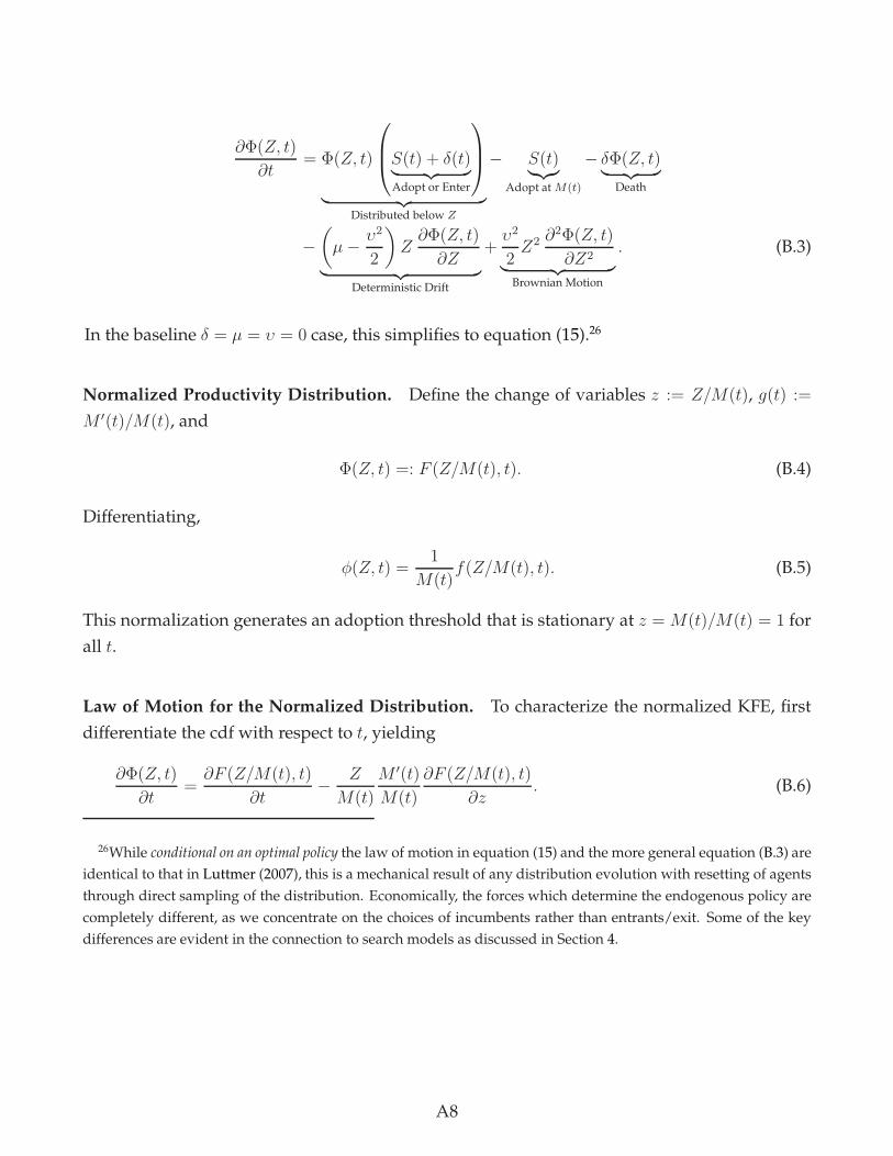
∂Φ(Z, t)
∂t= Φ(Z, t)
S(t) + δ(t)︸ ︷︷ ︸
Adopt or Enter
︸ ︷︷ ︸
Distributed below Z
− S(t)︸︷︷︸
Adopt at M(t)
− δΦ(Z, t)︸ ︷︷ ︸
Death
−
(
µ−υ2
2
)
Z∂Φ(Z, t)
∂Z︸ ︷︷ ︸
Deterministic Drift
+υ2
2Z2 ∂
2Φ(Z, t)
∂Z2︸ ︷︷ ︸
Brownian Motion
. (B.3)
In the baseline δ = µ = υ = 0 case, this simplifies to equation (15).26
Normalized Productivity Distribution. Define the change of variables z := Z/M(t), g(t) :=
M ′(t)/M(t), and
Φ(Z, t) =: F (Z/M(t), t). (B.4)
Differentiating,
φ(Z, t) =1
M(t)f(Z/M(t), t). (B.5)
This normalization generates an adoption threshold that is stationary at z = M(t)/M(t) = 1 for
all t.
Law of Motion for the Normalized Distribution. To characterize the normalized KFE, first
differentiate the cdf with respect to t, yielding
∂Φ(Z, t)
∂t=
∂F (Z/M(t), t)
∂t−
Z
M(t)
M ′(t)
M(t)
∂F (Z/M(t), t)
∂z. (B.6)
26While conditional on an optimal policy the law of motion in equation (15) and the more general equation (B.3) are
identical to that in Luttmer (2007), this is a mechanical result of any distribution evolution with resetting of agents
through direct sampling of the distribution. Economically, the forces which determine the endogenous policy are
completely different, as we concentrate on the choices of incumbents rather than entrants/exit. Some of the key
differences are evident in the connection to search models as discussed in Section 4.
A8

Differentiating the cdf with respect to Z yields
∂Φ(Z, t)
∂Z=
1
M(t)
∂F (Z/M(t), t)
∂z, (B.7)
∂2Φ(Z, t)
∂Z2=
1
M(t)2∂2F (Z/M(t), t)
∂z2. (B.8)
Given that z := ZM(t)
and g(t) := M ′(t)/M(t), combining equations (B.3), (B.6), (B.7), and (B.8)
provides the KFE in cdfs of the normalized distribution:
∂F (z, t)
∂t= (S(t) + δ(t)− δ)F (z, t) +
(g(t)− µ+ υ2/2
)z∂F (z, t)
∂z+
υ2
2z2∂2F (z, t)
∂z2− S(t).
(B.9)
The interpretation of this KFE is that while non-adopting incumbent firms are on average not
moving in absolute terms, they are moving backwards at rate g(t) relative to M(t) (adjusted for
the growth rate of the stochastic process). As the minimum of support is z = M(t)/M(t) = 1 for
all t, a necessary condition is that F (1, t) = 0 for all t, and therefore ∂F (1,t)∂t
= 0. Thus, evaluating
equation (B.9) at z = 1 gives an expression for S(t),27
S(t) =
(
g(t)− µ+υ2
2
)∂F (1, t)
∂z+
υ2
2
∂2F (1, t)
∂z2. (B.10)
This expression includes adopters caught by the boundary moving relative to their drift, as well
as the flux from the GBM pushing some of them over the endogenously determined threshold.
If µ = υ = δ = 0, then a truncation at M(t) solves equation (B.9) for any t and for any initial
condition, as in Perla and Tonetti (2014).
φ(Z, t) =φ(Z, 0)
1− Φ(M(t), 0). (B.11)
The only non-degenerate stationary F (z) consistent with equation (B.11) is given by equation
(B.13)—the same form as that with υ > 0.
The Stationary Normalized Productivity Distribution. From equation (B.9), the stationary
KFE is
0 = SF (z) +
(
g − µ+υ2
2
)
zF ′(z) +υ2
2z2F ′′(z)− S. (B.12)
27Equivalently, the flow of adopters can be derived as the net flow of the probability current through the adop-
tion threshold.
A9

subject to F (1) = 0 and F (∞) = 1.
Moreover, for any strictly positive υ > 0, the KFE will asymptotically generate a stationary
Pareto distribution for some tail parameter from any initial condition. While many θ > 1 could
solve this differential equation, the particular θ tail parameter is determined by initial condi-
tions and the evolution of M(t). As in Luttmer (2007) and Gabaix (2009), the geometric random
shocks leads to an endogenously determined power-law distribution.
F (z) = 1− z−θ. (B.13)
From equations B.12 and B.13, evaluating at z = 1 for a given g and θ,
S = θ
(
g − µ− θυ2
2
)
(B.14)
Therefore, given an equilibrium g and θ, the CDF in equation (B.13) and S from equation (B.14)
characterize the stationary distribution. The relationship between g and θ is determined by the
firms’ decisions given S and F (z). It is independent of δ on a BGP since the exit rate is constant
and uniform across firms (in contrast to Luttmer (2007), where selection into exit is generated
by fixed costs of operations and is not independent of firm productivity).
The Stationary Distribution with no GBM. For υ = 0, the lack of random shocks means
that the stationary distribution will not necessarily become a Pareto distribution from arbitrary
initial conditions. However, if the initial distribution is Pareto, the normalized distribution
will be constant. If the initial distribution is a power-law, then the stationary distribution is
asymptotically Pareto.
Since a Pareto distribution is attained for any υ > 0, we consider our baseline (υ = 0, µ = 0) case
with an initial Pareto distribution as a small noise limit of the full model with GBM from some
arbitrary initial condition. Beyond endogenously determining the tail index and changing the
expected time to execute the adoption option, exogenous productivity volatility of incumbent
firms has qualitatively little impact on the model. For the baseline case, from equation (B.14),
the flow of adopters is S = θg.
C. Normalized Static Equilibrium Conditions
To aid in computing a balanced growth path equilibrium, in this section we transform the
problem and derive normalized static equilibrium conditions.
A10

Expectations using the Normalized Distribution. If an integral of the following form exists,
for some unary function Ψ(·), substitute for f(z) from B.5, then do a change of variables of
z = ZM
to obtain a useful transformation of the integral.
∫∞
M
Ψ(
ZM
)φ(Z)dZ =
∫∞
M
Ψ(
ZM
)f(
ZM
)1MdZ =
∫∞
M/M
Ψ(z)f(z)dz. (C.1)
The key to this transformation is that moving from φ to f introduces a 1/M term. Thus, abusing
notation by using an expectation of the normalized variable,
∫∞
M
Ψ(
ZM
)φ(Z)dZ = E [Ψ(z)] . (C.2)
C.1. Normalizing the Static Equilibrium
Define the following normalized, real, per-capita values: z := ZM, y := Y
LMP, c := C
LM, qd(Z) :=
Qd(Z)LM
, x := XLMw
, w := WMP
and πd(Z) :=Πd(Z)LMw
. Note the normalization of profits and adoption
costs is relative to real, normalized wages.
Combining the normalized variables with equations (A.8) and (A.9) provides the real prices in
terms of real, normalized wages.
pd(Z)P
= σ wZ/M
, (C.3)px(Z)P
= σd wZ/M
. (C.4)
Substituting equations (C.3) and (C.4) into equation (A.4) and dividing by LM yields normal-
ized quantities,
qd(Z) = σ−σw−σy(
ZM
)σ, (C.5)
qx(Z) = σ−σw−σd−σy(
ZM
)σ. (C.6)
Divide equation (A.10) by L, then substitute from equations (A.4) and (C.3). Finally, divide the
top and bottom by M to obtain normalized demand for production labor
ℓd(Z)/L = σ−σw−σy(
ZM
)σ−1, (C.7)
ℓx(Z)/L = σ−σw−σyd1−σ(
ZM
)σ−1. (C.8)
Divide equation (A.5) by P 1−σ and then substitute from equation (C.3) for pd(Z)/P to obtain
1 = Ωσ1−σw1−σ
[∫∞
M
(ZM
)σ−1dΦ(Z) + (N − 1)
∫∞
Z
d1−σ(
ZM
)σ−1dΦ(Z)
]
. (C.9)
A11

Simplify equation (C.9) by defining z, a measure of effective aggregate productivity. Then use
equation (C.2) to give normalized real wages in terms of parameters, z, and the productivity
distribution
z :=[Ω(E[zσ−1
]+ (N − 1)(1− F (z))d1−σ
E[zσ−1|z > z
])] 1σ−1 , (C.10)
wσ−1 = σ1−σzσ−1, (C.11)
w = 1σz. (C.12)
Note that if d = 1 and z = 1, then w = 1σ(ΩNE [z1−σ])
1/(σ−1). Divide equations (A.11) and (A.12)
by LMw and substitute with equation (C.11) to obtain normalized profits,
πd(Z) =1σ
(p(Z)P
)1−σyw= 1
σzσ−1yw
(ZM
)σ−1, (C.13)
πx(Z) =1
σzσ−1ywd1−σ
(ZM
)σ−1− κ. (C.14)
Divide equations (A.15) and (A.16) by LMw and use equations (C.13) and (C.14) to find aggre-
gate profits from domestic production and from exporting to one country,
πd = Ω 1σzσ−1
ywE[zσ−1
], (C.15)
πx = Ω(
1σzσ−1
ywd1−σ(1− F (z))E
[zσ−1|z > z
]− (1− F (z))κ
). (C.16)
Divide equation (A.25) by L, and aggregate the total labor demand from equations (C.7) and
(C.8) to obtain normalized aggregate labor demand
1 = Ωσ−σw−σy(E[zσ−1
]+ (N − 1)(1− F (z))d1−σ
E[zσ−1|z > z
])
+ Ω(N − 1)(1− F (z))κ+ Ω(1− η)ζS (C.17)
= σ−σw−σyzσ−1 + Ω((N − 1)(1− F (z))κ + (1− η)ζ (S + δ/χ)) . (C.18)
Define L as a normalized quantity of labor used outside of variable production. Multiply equa-
tion (C.18) by w, and use equation (C.11) to show that
L := Ω [(N − 1)(1− F (z))κ+ (1− η)ζ (S + δ/χ)] , (C.19)
w = 1σy + Lw, (C.20)
1 = 1σ
yw+ L. (C.21)
A12

Reorganize to find real output as a function of the productivity distribution and labor supply
(net of labor used for the fixed costs of exporting and adopting technology)
yw= σ
(
1− L)
, (C.22)
y =(
1− L)
z. (C.23)
This equation lends interpretation to z as being related to the aggregate productivity. Substi-
tuting equation (C.22) into equations (C.13) and (C.14) to obtain a useful formulation of firm
profits
πd(Z) =1−L
(σ−1)zσ−1
(ZM
)σ−1, (C.24)
πx(Z) =1−L
(σ−1)zσ−1d1−σ(
ZM
)σ−1− κ. (C.25)
Define the common profit multiplier πmin as
πmin := 1−L(σ−1)zσ−1 = 1−L
(σ−1)(σw)σ−1 =(σw)1−σy
σw, (C.26)
πd(Z) = πmin
(ZM
)σ−1, (C.27)
πx(Z) = πmind1−σ(
ZM
)σ−1− κ. (C.28)
Use equation (C.28) set to zero to solve for z. This is an implicit equation as πmin is a function of
z through z
z = d(
κπmin
) 1σ−1
. (C.29)
Substitute equations (C.27) and (C.28) into equations (C.15) and (C.16) to obtain a useful for-
mulation for aggregate profits
πd = ΩπminE[zσ−1
], (C.30)
πx = Ω((1− F (z))
(πmind
1−σE[zσ−1|z > z
]− κ))
. (C.31)
Combine to calculate aggregate total profits
πd + (N − 1)πx = Ωπmin
[E[zσ−1
]+ (N − 1)(1− F (z))d1−σ
E[zσ−1|z > z
]]
− Ω(N − 1)(1− F (z))κ. (C.32)
A13

Rewriting aggregate total profits using the definition of z yields
πagg := πminzσ−1 − Ω(N − 1)(1− F (z))κ. (C.33)
Note that in a closed economy, z = (ΩE [zσ−1])1/(σ−1) and therefore aggregate profits relative to
wage are a markup dependent fraction of normalized output relative to wage πd = 1−Lσ−1
. Take
the resource constraint in equation (A.26) and divide by MLw and then use equation (C.22) to
get an equation for normalized, per-capita consumption
cw= y
w− ΩηζΘ (S + δ/χ) /w = σ
(
1− L)
− Ωηζ Θw(S + δ/χ) , (C.34)
c =(
1− L)
z − ηζΩΘ (S + δ/χ) . (C.35)
Normalize the cost in equation (A.23) by dividing by LPMw. This is implicitly a function of z
through w
x = ζ (1− η + ηΘ/w) . (C.36)
Normalize the trade share in equation (A.17) by substituting from equations (C.4) and (C.11)
λ = (1− F (z))d1−σΩE [zσ−1|z > z]
zσ−1. (C.37)
Starting from C.33, use C.26, and C.19, to derive that
πagg =1
σ − 1(1− Ω [(1− η)ζ (S + δ/χ)− σ(N − 1)(1− F (z))κ]) . (C.38)
Stationary Trade Shares and Profits. Using the stationary distribution in equation (B.13), cal-
culate average profits from C.33,
πagg
Ω=
πminθ
1 + θ − σ+
(σ − 1)(N − 1)κz−θ
1 + θ − σ. (C.39)
Note that the minimum profits are at z = 1 and equal to πmin as long as z > 1. Using this to
define the profit spread between the average and worst firm in the economy,
πagg
Ω− πmin =
πminθ
1 + θ − σ+
(σ − 1)(N − 1)κz−θ
1 + θ − σ− πmin
︸ ︷︷ ︸
ProfitSpread
=(σ − 1)πmin
1 + θ − σ+
(σ − 1)(N − 1)κz−θ
1 + θ − σ.
(C.40)
A14

Define the ratio of mean to minimum profits as πrat :=π/Ωπmin
. From C.40 and C.29 find that
πrat =θ
1 + θ − σ+ (N − 1)d1−σ (σ − 1)zσ−1−θ
1 + θ − σ. (C.41)
Take equations (C.37) and (C.10) to find
zσ−1 = ΩE[zσ−1
]+ (N − 1)λzσ−1. (C.42)
Solving gives an expression for a function of aggregate productivity in terms of underlying
productivity and trade shares. Defining the home trade share as λii := 1− (N − 1)λ,
zσ−1 = ΩE [zσ−1]
1− (N − 1)λ= Ω
E [zσ−1]
λii
. (C.43)
From equations (C.12) and (C.43),
w =1
σΩ
11−σE
[zσ−1
] 1σ−1 λ
11−σ
ii . (C.44)
This relates the real normalized wage to the aggregate productivity, the home trade share, and
the number of varieties. Given that σ > 1, this expression implies that the larger the share of
goods purchased at home, the lower the real wage is.
From C.37 and C.43 ,
λ = (1− F (z))d1−σE [zσ−1|z > z]λii
E [zσ−1]. (C.45)
Using the stationary distribution,
λ = z−θd1−σzσ−1 θ
θ−(σ−1)λii
θθ−(σ−1)
= z−θd1−σzσ−1λii. (C.46)
Using the definition of the home trade share,
λii =1
1 + (N − 1)zσ−1−θd1−σ. (C.47)
Furthermore, multiplying the numerator and denominator by πmin and using equation (C.29),
λii =πmin
πmin + (N − 1)z−θκ. (C.48)
A15

Which gives an alternative expression for πmin when κ > 0,
πmin =(N − 1)z−θκ
1− λii. (C.49)
D. Normalized and Stationary Dynamic Equilibrium Conditions
This section derives normalized stationary dynamic balanced growth path equilibrium condi-
tions.
D.1. Utility and Welfare on a BGP
Using the substitution C(t) = cLM(t) shows time 0 welfare U as a function of c and g is
U(c, g) = 11−γ
(cLM(0))1−γ
ρ+(γ−1)g. (D.1)
With log utility
U(c, g) =ρ log(cLM(0)) + g
ρ2. (D.2)
Using the standard IES of the consumer, adjusted for stochastic death of the firm, the interest
rate on a BGP is,
r = ρ+ γg + δ. (D.3)
With log utility
r = ρ+ g + δ. (D.4)
We restrict parameters such that g(1 − γ) < ρ in equilibrium to ensure finite utility. In the log
utility case, this is simply ρ > 0.
D.2. Normalization of the Firm’s Dynamic Problem
We proceed to derive the normalized continuation value function, value matching condition,
and smooth pasting condition originally specified in equations (A.20)–(A.22). Define the nor-
malized real value of the firm relative to normalized wages as
v(z, t) := V (Z,t)LM(t)w(t)
. (D.5)
A16
Rearranging
V (Z, t) = Lw(t)M(t)v(Z/M(t), t). (D.6)
First differentiate the continuation value V (Z, t) with respect to t in equation (D.6) and divide
by w(t)M(t)L, using the chain and product rule. This gives,
1
w(t)M(t)L
∂V (Z, t)
∂t=
M ′(t)
M(t)v(z, t)−
M ′(t)
M(t)
Z
M(t)
∂v(z, t)
∂z+
M(t)
M(t)
∂v(z, t)
∂t+
w′(t)
w(t)v(z, t).
(D.7)
Defining the growth rate of g(t) := M ′(t)/M(t) and gw(t) := w′(t)/w(t). Substitute these into
equation (D.7), cancel out M(t), and group z = Z/M(t) to give
1
w(t)M(t)L
∂V (Z, t)
∂t= (g(t) + gw(t))v(z, t)− g(t)z
∂v(z, t)
∂z+
∂v(z, t)
∂t. (D.8)
Differentiating equation (D.6) with respect to Z yields
∂V (Z, t)
∂Z=
LM(t)w(t)
M(t)
∂v(Z/M(t), t)
∂z= Lw(t)
∂v(z, t)
∂z. (D.9)
Similarly,
∂2V (Z, t)
∂Z2=
Lw(t)
M(t)
∂2v(z, t)
∂z2. (D.10)
Define the normalized profits from equation (A.19) as
π(z, t) :=Π(zM(t), t)
w(t)M(t)L. (D.11)
Divide equation (A.20) by M(t)w(t)L, then substitute for ∂V (Z,t)∂t
, ∂V (Z,t)∂Z
, and ∂2V (Z,t)∂Z2 from eqs.
(D.8), (D.9), and (D.10) in to (A.20). Finally, group the normalized profits using equation (D.11):
(r(t)− g(t)− gw(t))v(z, t) = π(z, t) +
(
µ+υ2
2− g(t)
)
z∂v(z, t)
∂z+
υ2
2z2∂2v(z, t)
∂z2+
∂v(z, t)
∂t.
(D.12)
Equation (D.12) is the normalized version of the value function of the firm in the continuation
A17

region. The stationary version of this equation is,
(r − g)v(z) = π(z) +
(
µ+υ2
2− g
)
zv′(z) +υ2
2z2v′′(z). (D.13)
To derive the normalized smooth pasting condition, use equation (A.22) to show that equation
(D.9) evaluated at Z = M(t) equals 0, delivering
∂v(1, t)
∂z= 0. (D.14)
To arrive at the normalized value matching condition, divide equation (A.21) by M(t)w(t)L to
obtain
V (M(t), t)
M(t)w(t)L=
∫∞
M(t)
V (Z, t)
M(t)w(t)Lφ(Z, t)dZ −
X(t)
M(t)w(t)L(D.15)
Substituting using equation (D.5) and the definition of x(t) yields
v(M(t)/M(t), t) =
∫∞
M
v(Z/M, t)φ(Z, t)dZ − x(t). (D.16)
Finally, normalize the integral, realizing it is of the form discussed in equation (C.2), to obtain
the normalized value matching condition:
v(1, t) =
∫∞
1
v(z, t)f(z, t)dz − x(t). (D.17)
D.3. Normalization of the Free Entry Condition
Normalizing the free entry condition given in equation (A.24), following similar steps that
delivered the normalized value matching condition in equation (D.17), gives
x(t)/χ =
∫∞
1
v(z, t)f(z, t)dz. (D.18)
Relating this to the value-matching condition of the adopting firm given in equation (D.17) pro-
vides a simple formulation of the stationary free entry condition that is useful in determining
Ω and g:
v(1) = x1− χ
χ. (D.19)
A18

E. Solving for the Continuation Value Function
Although our baseline model does not feature exogenous productivity shocks, in this section
we solve for the value function of a more general model that has GBM with υ ≥ 0. Our baseline
case of υ = 0 is nested in this formulation. The differential equation for the value function is
solved using the method of undetermined coefficients. The goal of this section is to solve for
the value function as a function of parameters, g, Ω, and z (sometimes implicitly through πmin).
Selection into Exporting. If κ > 0, generically some firms will choose to be exporters and
some firms will only sell domestically. The value function will have a region of productivities
representing the value of firms that only sell domestically and a region representing firms that
also export. That is,
v(z) =
vd(z) if z ≤ z
vx(z) if z ≥ z.
We guess the value function is of the following form, with undetermined constants a, ν, and
b,28
vd(z) = aπmin
(
zσ−1 +σ − 1
νz−ν
)
, (E.1)
vx(z) = aπmin
(
(1 + (N − 1)d1−σ)zσ−1 +σ − 1
νz−ν + (N − 1)
1
a(r − g)
(
bz−ν −κ
πmin
))
. (E.2)
The value of a firm can be decomposed into the value of operating with its current productivity
forever and the option value of adopting a better technology. The constant a is a discounting
term on the value of earning the profits from producing with productivity z in perpetuity. The
constant ν reflects the rate at which the option value of technology adoption goes to zero as
productivity increases. The constant b is an adjustment to the perpetuity profits that reflects a
firm with productivity z will eventually switch from exporting to being a domestic producer if
z is constant in a growing economy.
By construction, the form of these guesses ensures that value matching and smooth pasting are
satisfied, both at the adoption threshold (z = 1) and the exporter threshold (z = z). To solve
for a and ν, substitute equation (E.1) into the continuation value function in equation (D.13)
using πd(z) from equation (C.27). This generates an ODE and, grouping terms, the method of
28This guess is also applying a standard transversality condition to eliminate an explosive root.
A19

undetermined coefficients provides a system of 2 equations in the 2 unknowns.29
Solving the system gives,
ν =µ− g
υ2+
√(g − µ
υ2
)2
+r − g
υ2/2, (E.3)
a =1
r − g − (σ − 1)(µ− g + (σ − 1)υ2/2). (E.4)
To solve for b, plug equation (E.2) into the continuation value function in equation (D.13) using
πx(z) from equation (C.28). This generates an ODE and, grouping terms, the method of unde-
termined coefficients provides a system of 3 equations in the 3 unknowns. By construction, the
a and ν terms match those previously found, giving a consistent solution for b:
b = (1− a(r − g)) d1−σzν+σ−1. (E.5)
Note, the main effect of the GBM is to modify the ν constant to reflect changes in the expected
execution time of the option value of technology diffusion, and hence the exponent for dis-
counting.
As will be useful in solving for g, evaluating at the adoption threshold yields,
v(1) = aπmin
(
1 +σ − 1
ν
)
. (E.6)
For the baseline case of µ = υ = 0,
a =1
r + (σ − 2)g, (E.7)
ν =r
g− 1, (E.8)
b =σ − 1
ν + σ − 1d1−σzν+σ−1. (E.9)
29Instead of the method of undetermined coefficients, a direct solution approach would be to solve the continu-
ation value function ODEs in the domestic sales and exporter regions, using the smooth pasting condition as the
boundary value.
A20

F. Computing the BGP Equilibrium when All Firms Export
In the case of κ = 0 all firms export (given d s.t. the economy is not in autarky), and the value
function has only one region. We guess that the value function will take the following form,
v(z) = aπmin
(1 + (N − 1)d1−σ
)(
zσ−1 +σ − 1
νz−ν
)
. (F.1)
Substituting equation (F.1) into the continuation value function in equation (D.13) with profits
from equation (C.28), the ν and a are identical to those from equations (E.3) and (E.4). Evaluat-
ing at the threshold,
v(1) = a(1 + (N − 1)d1−σ
)πmin
(
1 +σ − 1
ν
)
. (F.2)
Solving for the Growth Rate and Mass of Varieties when All Firms Export. Using the free
entry condition from equation (D.19) with equation (F.2) to find,
x
πmin
= a(1 + (N − 1)d1−σ
) χ
1− χ
σ + ν − 1
ν. (F.3)
Substitute equations (F.1) and (F.2) into the value matching condition of equation (D.17), and
divide by aπmin(1 + (N − 1)d1−σ)
1 +σ − 1
ν=
θ(ν + σ − 1)(θ + ν − σ + 1)
ν(θ + ν)(θ − σ + 1)−
x
πmina (1 + (N − 1)d1−σ). (F.4)
Combine equations (F.3) and (F.4), and solve for ν. For any cost function x and minimum profits
πmin,
ν =χθ(θ + 1− σ)
σ − 1− θχ. (F.5)
The aggregate growth rate is found by equating equations (E.3) and (F.5) to find
g = µ︸︷︷︸
Drift
+(r − µ)((σ − 1)/χ− θ)
θ2 − θσ + (σ − 1)/χ︸ ︷︷ ︸
Deterministic
+υ2
2
θ2(θ + 1− σ)2
(θ2 − θσ + (σ − 1)/χ)(θ − (σ − 1)/χ)︸ ︷︷ ︸
Stochastic
. (F.6)
In the baseline case of υ = µ = 0
g =(ρ+ δ)(σ − 1− χθ)
θχ(γ + θ − σ)− (γ − 1)(σ − 1), (F.7)
A21

and,
x
πmin=(1 + (N − 1)d1−σ
) χ
1− χ
1
r − g. (F.8)
The growth rate is independent of the trade costs, the population, and the number of countries.
The intuition–as discussed in the body of the paper–is that the growth rate is driven by the ratio
of the minimum to the mean profits, which are proportional and independent of the scale or
integration of economies in the absence of any export selection. The constant death rate only
enters to increase the discount rate.
Note in the baseline case of υ = µ = δ = 0 and log utility
g =ρ(σ − 1− χθ)
θ2χπk
rat, (F.9)
where (from eqs. C.33 and C.10 with κ = 0 and z = 1) the ratio of average profits to minimum
profits is
πkrat =
πkagg/Ω
πkmin
=(1 + (N − 1)d1−σ)πminE[zσ−1]
(1 + (N − 1)d1−σ)πmin= E[zσ−1] =
θ
1 + θ − σ. (F.10)
The Mass of Varieties Ω. Here we solve for the mass of varieties Ω in the baseline case of
υ = µ = δ = 0.
Substitute into the free entry condition equation (F.8) using the definition of πmin in terms of
z and L from equation (C.26), the definition of z from equation (C.10), and the definition of
L from equation (C.19), to obtain the implicit equation. In the baseline case where η = 0, an
explicit solution is30
Ω =χ((γ − 1)(σ − 1)− θχ(γ + θ − σ))
ζ (θχ(−γδ − σ(θ(δ + ρ) + ρ) + δ + θρ+ ρ) + (γ − 1)δ(σ − 1) + θ2σχ2(δ + ρ)). (F.13)
Note that the only place that the adoption cost, ζ , has come into the system of Ω and g is in the
denominator of F.13. For this reason, the ζ parameter (along with L) determines the scale of the
30The solution for the simplest case of γ = 1 and δ = 0 is,
g =ρ(σ − 1− θχ)
θχ(1 + θ − σ)(F.11)
Ω =χ(1 + θ − σ)
ζρ ((1 + θ)(σ − 1)− σθχ)(F.12)
A22

economy.
It can be shown that in the Krugman model for all cases with η = 0, the number of domestic
varieties is independent of trade costs d. Thus, both Ω and g are independent of d if η = 0. This
implies through equations (C.19) and (B.14) that the amount of labor dedicated to technology
adoption, L, is also independent of d if η = 0.
Through C.35, since L, Ω, and g are independent of d when η = 0, in response to a decrease in
trade costs d, c increases only due to the (1 + (N − 1)d1−σ)1/(σ−1) term in z.
The key relationship can be summarized by the following elasticities.
∂ log πkrat(d)
∂ log d= 0. (F.14)
Using equation (C.47) with z = 1 shows
∂ log λii(d)
∂ log d= (σ − 1)
(
1 +dσ−1
N − 1
)−1
= (σ − 1)(1− λii) > 0. (F.15)
Furthermore, when η = 0,
∂ log(1− L(d))
∂ log d=
∂ log Ω(d)
∂ log d=
∂ log g(d)
∂ log d= 0. (F.16)
For the case with η = 0, the ratio of c for different trade costs d1 and d2 that both feature positive
trade is
cd1cd2
=zzd1zd2
=
(1 + (N − 1)d1−σ
1
1 + (N − 1)d1−σ2
) 1σ−1
. (F.17)
Using the normalized welfare function in equation (D.1), since g is independent of d in the κ = 0
case, the ratio of welfare for different trade costs d1 and d2 that both feature positive trade (for
γ > 0) is,
Ud1
Ud2
=
(1 + (N − 1)d1−σ
1
1 + (N − 1)d1−σ2
) 1−γσ−1
. (F.18)
Comparing welfare between free trade (d = 1) and autarky (sufficiently high d s.t. there are no
exporters) gives (for γ 6= 1)
Ufree
Uautarky
= N1−γσ−1 . (F.19)
A23

G. Computing the BGP Equilibrium with Selection into Exporting (κ > 0)
We solve for g and Ω by reducing the equilibrium conditions to a system of two equations in
these two unknowns. First, combining the free entry condition from equation (D.19) with v(1)
from equation (E.6) yields
x
πmin
= aχ
1− χ
σ + ν − 1
ν. (G.1)
The second equation is found by evaluating the value matching condition of equation (D.17) by
substituting in the domestic and exporter value functions in equations E.1 and E.2, the export
threshold z in equation (C.29), and the value at the adoption threshold v(1) in equation (E.6)
and dividing by aπmin. That is, evaluate
v(1)
aπmin
=
∫∞
1v(z, t)f(z, t)dz
aπmin
−x
aπmin
(G.2)
to obtain
1 +σ − 1
ν=
ν(n−1)(θ−σ+1)(d1−σ(θ+ν)z−θ+σ−1−bθz−θ−ν)
a(g−r)+θ(ν(n−1)d1−σ (θ+ν)z−θ+σ−1+(ν+σ−1)(θ+ν−σ+1))
ν(θ+ν)(θ−σ+1)−
χ1−χ
σ+ν−1ν
.
(G.3)
As detailed in Section H, use the definition of πmin and substitute for x, ν, a, b, z and r into equa-
tions (G.1) and (G.3) to find a system of 2 equations in Ω and g. Note that the adoption cost x
does not appear in equation (G.3), which is why g is independent of the specification of the cost
of adoption. Equation (G.1) does explicitly depend on x, which is why the number of varieties
is a function of the adoption cost, and ultimately why welfare is also a function of x.
G.1. Case with υ = µ = δ = 0
As the GBM does not qualitatively impact the solution, we concentrate our analytical theory
on the simple baseline case. The cost of adoption is a function of minimum profits, parameters,
and r − g:
x = πminχ
1− χ
1
r − g. (G.4)
Evaluating the general equation (G.3) with the substitutions for x, ν, a, b, z and r that correspond
to the baseline case of υ = µ = δ = 0 yields a unique g that satisfies the value function and the
A24

value matching equations, given by the implicit equation,
g =
(σ − 1 + (N − 1)θd1−σz−θ+σ−1
)πmin + (N − 1)(−θ + σ − 1)z−θκ
x(γ + θ − 1)(θ − σ + 1)−
ρ
γ + θ − 1. (G.5)
Using κ/πmin = zσ−1d1−σ from equation (C.29), simplify to
g =(σ − 1)
[πmin + (N − 1)κz−θ
]
x(γ + θ − 1)(θ − σ + 1)−
ρ
γ + θ − 1. (G.6)
Using equation (C.40), realize this relates the growth rate to the difference between average and
minimum profits
g =
(πagg/Ω− πmin
x(γ + θ − 1)
)
−ρ
γ + θ − 1. (G.7)
Substitute for x using the free entry condition in equation (G.4), use the definition of the average
to minimum profit ratio(
πrat :=π/Ωπmin
)
, and substitute for r using equation (D.3) to obtain
g = (ρ+ (γ − 1)g)1− χ
χ(γ + θ − 1)(πrat − 1)−
ρ
γ + θ − 1. (G.8)
Solving for g gives an equation for g as a function exclusively of parameters and the ratio of
average to minimum profits
g =ρ
χθ ((1− χ)πrat − 1)−1 + 1− γ. (G.9)
Furthermore, with log utility γ = 1 and
g =ρ(1− χ)
χθπrat −
ρ
χθ. (G.10)
The relationship between growth and trade costs. First, note that the growth rate is increas-
ing in the profit ratio, (since χ ∈ (0, 1)):
dg(πrat)
dπrat=
ρθχ(1− χ)
((γ − 1)(1− (1− χ)πrat + θχ)2> 0. (G.11)
To determine if whether growth is increasing in d, use the chain rule
dg(d)
dd=
dg(πrat)
dπrat
dπrat(d)
dd. (G.12)
A25

Given equations (G.11) and (G.12), a sufficient condition to conclude that dg(d)dd
< 0 is dπrat(d)dd
< 0.
To show this differentiate C.41 w.r.t. d to find,
dπrat(d)
dd∝ −
(
(σ − 1)z(d) + d(1 + θ − σ)dz(d)
dd
)
. (G.13)
Since d > 0, z(d) > 0, σ > 1, and 1+ θ− σ > 0, a sufficient condition for dπrat(d)dd
< 0 is if dz(d)dd
> 0.
Differentiate equation (C.29) to find
dz(d)
dd∝ (σ − 1)−
d
πmin(d)
dπmin(d)
dd. (G.14)
Therefore, a sufficient condition to conclude that dz(d)dd
> 0 is
d log πmin(d)
dd<
σ − 1
d. (G.15)
Summarizing,
signdg(d)
dd= sign
dπrat
dd= −sign
dz(d)
dd. (G.16)
G.2. Baseline Case with υ = µ = δ = η = 0 and log utility.
Adding the restriction that η = 0 and γ = 1 to the adoption cost equation (C.36) and the interest
rate equation (D.4) delivers the key simplifications that permit solving for the BGP equilibrium
in closed form:
Calculating the Growth Rate and the Mass of Varieties.
x = ζ, (G.17)
r − g = ρ. (G.18)
Using equation (G.4) gives an expression for πmin in terms of model parameters
πmin =(1− χ)ζρ
χ. (G.19)
Substitute equation (G.19) into equation (C.29) to find the export threshold in terms of param-
eters,
z = d
(1
ζ
κχ
ρ(1− χ)
) 1σ−1
. (G.20)
A26

Substitute γ = 1 and equations (G.17), (G.19), and (G.20) into equation (G.6) and simplify to
obtain g in closed form:
g =ρ(1 − χ)
χθ
σ − 1
(θ − σ + 1)
(
1 + (N − 1)d−θ
(κ
ζ
χ
ρ(1− χ)
)1− θσ−1
)
−ρ
θ, (G.21)
=ρ(1 − χ)
χθ
(
θ + (N − 1)(σ − 1)d−θ(
1ζ
κχρ(1−χ)
)1− θσ−1
)
(θ − σ + 1)−
ρ
χθ. (G.22)
For ease of comparison to g as a function of πrat use equation (G.8) evaluated at γ = 1 with
equation (G.21) to realize
πrat − 1 =
(
1 + (N − 1)d−θ(
1ζ
κχρ(1−χ)
)1− θσ−1
)
(θ
σ−1− 1) , (G.23)
or equation (G.10) with equation (G.22) to see
πrat =
(
θ + (N − 1)(σ − 1)d−θ(
1ζ
κχρ(1−χ)
)1− θσ−1
)
(θ − σ + 1). (G.24)
Note, g is decreasing in d and κ (since θ > 0, σ > 1, and 1 + θ − σ > 0). Thus, from equation
(G.16) or direct differentiation of equation (G.21),
dg
dd< 0;
dπrat
dd< 0;
dz
dd> 0;
dg
dκ< 0. (G.25)
See by comparing to equation (F.7) that the limit of g as d → ∞ in equation (G.22) equals the
autarky and all-export economy growth rates, so there is no discontinuity in the economy in
this direction.
Note that the parameter ζ (previously interpreted as the scale in equation F.13) and κ only enter
the growth rate multiplicatively. This is because the fixed costs of adoption, entry, and export in
levels are proportional to the scale of the economy. Since the calibration strategy targets relative
moments (i.e., proportion of exporters, relative size of exporters to domestic firms, growth rates,
trade shares), κ is not separately identifiable from ζ without some moment that targets the level
of the economy.
To find the number of varieties, maintain γ = 1, η = 0. To solve for Ω, start with the definition
of πmin from equation (C.26):
πmin =1−L
(σ−1)zσ−1 . (G.26)
A27

For πmin, substitute from equation (G.19). For the right hand side, substitute for L, z and S with
equations (C.19), (C.10), and (B.14). Then, use g and z from equations (G.21), (G.20), and solve
for Ω in terms of model parameters:
Ω =1
ζ
χ(1 + θ − σ)
(1− χ)θσρ
(
1 + (N − 1)d−θ
(κχ
ζρ(1− χ)
)1− θσ−1
−1 + θ − σ
θσ(1− χ)
)−1
. (G.27)
Note, from equations (C.47) and (G.20), the home trade share is,
λii =1
1 + (N − 1)d−θ(
κχζρ(1−χ)
)1− θσ−1
. (G.28)
Note, using eqs. G.21 and G.29, the growth rate and Ω can be written as a function of the home
trade share:
g =ρ(1− χ)
χθ
σ − 1
(θ − σ + 1)λ−1ii −
ρ
θ. (G.29)
Ω =χ
ζρ
((1− χ)θσ
1 + θ − σλ−1ii − 1
)−1
. (G.30)
Calculating Consumption. By the resource constraint, c = y when η = 0 (equation C.34).
Thus, using equation (C.23), consumption is given by
c = y = (1− L)z. (G.31)
Equations (C.19), (B.14), (C.29), and (G.29) combine to yield the amount of labor dedicated to
variable goods production in terms of the home trade share:
1− L = (σ − 1)
(
σ −1 + θ − σ
θ(1− χ)λii
)−1
. (G.32)
Equation (C.43) gives
z = Ω1
σ−1λ1
1−σ
ii
(E[zσ−1
]) 1σ−1 . (G.33)
Substituting equations (G.32), (G.33), and (G.30) into equation (G.31) yields consumption as a
function of parameters and the home trade share:
c =(σ − 1)θσ(1− χ)
σ(1 + θ − σ)
(χ
ρζ
) 1σ−1((1− χ)θσ
1 + θ − σ− λii
) σ1−σ (
E[zσ−1
]) 1σ−1 . (G.34)
A28

Trade Cost Elasticities. Comparative statics are analyzed by calculating elasticities with re-
spect to trade costs using equations (G.21), (G.27), and (G.28):
∂ log πrat(d)
∂ log d= −θ
1 +
θdθ(
κχζρ(1−χ)
) θσ−1
−1
(N − 1)(σ − 1)
−1
< 0, (G.35)
∂ log g(d)
∂ log d= −θ
1 +
ρdθ(−θχ+ σ − 1)(
κχζρ(1−χ)
) θσ−1
κ(N − 1)(σ − 1)χ
−1
< 0, (G.36)
∂ log Ω(d)
∂ log d= θ
1 +
ρdθ((θ + 1)(σ − 1)− θσχ)(
κχζρ(1−χ)
) θσ−1
θκ(N − 1)σχ
−1
> 0, (G.37)
∂ log λii(d)
∂ log d= θ
(
1 +dθ
N − 1
(κχ
ζρ(1− χ)
) θσ−1
−1)−1
> 0. (G.38)
Let εf,x be the elasticity of any f(x) w.r.t. x. These elasticities can be rearranged to highlight
their relationship to trade volume. To see this, first define the ratio of the home trade share to
the share of goods purchased away from home:
λii
1− λii=
dθ(
κχζρ(1−χ)
) θσ−1
−1
N − 1. (G.39)
Substituting this into the result above, yields
∂ log λii(d)
∂ log d= θ
(
1 +λii
1− λii
)−1
= θ(1− λii), (G.40)
∂ log g(d)
∂ log d= −θ
[
1 +
(−θχ + σ − 1
(σ − 1)(1− χ)
)λii
1− λii
]−1
(G.41)
=
(χ(1 + θ − σ)
(σ − 1)(1− χ)λii − 1
)−1
ελii,d, (G.42)
∂ log Ωii(d)
∂ log d=
(
1−1 + θ − σ
θσ(1− χ)λii
)−1
ελii,d. (G.43)
The elasticity of (1− L) w.r.t. d is
∂ log(1− L(d))
∂ log d=
(θσ(1− χ)
1 + θ − σλ−1ii − 1
)−1
ελii,d > 0. (G.44)
A29

The elasticity of z w.r.t. d is
∂ log(z(d))
∂ log d=
εΩ,d − ελii,d
σ − 1> 0. (G.45)
From equation (G.31)
εc,d = ε1−L,d + εz,d. (G.46)
Using equations (G.34) and (G.40) yields
εc,d = −σ
σ − 1
(
1−θσ(1− χ)
(1 + θ − σ)λ−1ii
)−1
ελii,d. (G.47)
Finally, from D.2
εU,d =ρ εc,d + g εg,d
g + ρ log(cLM(0))(G.48)
=ρ2
U(ρ εc,d + g εg,d). (G.49)
This can be further organized by substitution for εc,d and εg,d from equations (G.47) and (G.42)
into equation (G.49).31
εU ,d = −ελii,dρ3
U
σ
(σ − 1)(
1− θσ(1−χ)(θ−σ+1)λii
) +(σ − 1)(1− χ)
θχ(θ − σ + 1)λii
. (G.50)
Therefore, if the term in brackets is positive, then the elasticity of utility is of the opposite sign
of the home trade share, and hence always decreasing in trade costs.
Firm Adoption Timing. A firm adopts when normalized productivity equals 1 by definition.
On the BGP, firms drift backwards towards z = 1 at constant rate g. Thus, the time until
adoption τ(z) is given by
e−gτz = 1
τ(z) =log(z)
g(G.51)
31For determining the direction of the change, as an elasticity is dU ′(d)/U(d), and since d > 1, if U(d) > 0 then
the sign of this elasticity calculation matches the sign of the derivative. Otherwise, the sign of the derivative is
negative of the elasticity. As equation (G.49) divided by the utility in the calculation, this sign cancels, and ensures
that negative utility does not effect the direction of the changes (as expected with a monotone function with the
possibility of arbitrarily small initial conditions).
A30

The expected time until adoption for a firm that is about to draw a new productivity, τ , is just
the expected adoption time integrated over the distribution of the new z:
τ =
∫∞
1
log(z)
gdF (z) =
1
g
∫∞
1
log(z)θz−θ−1 =1
θg(G.52)
Since firms draw a new z from the unconditional distribution, the expected time to adoption
for a newly adopting firm is the same as the average time to adoption.
H. Computing the BGP Equilibrium in General
In the general case of the κ = 0, the equilibrium g can be calculated through an explicit equation,
and the Ω found separately. If κ > 0, then a system of 2 non-linear algebraic equations in g and
Ω are solved. Summarizing equations for easy reference against the code:
General Substitutions. The following substitutions are used in reducing the equilibrium con-
ditions into a simple system of equations that can be solved for g and Ω. Given g and Ω all other
equilibrium values are determined. We use equations (B.13), (B.14), (E.3), (E.4), (E.5), (D.3),
(C.19), (C.10), (C.29), (C.12), and (C.36):
F (z) = 1− z−θ (H.1)
S = θ
(
g − µ− θυ2
2
)
(H.2)
ν =µ− g
υ2+
√(g − µ
υ2
)2
+r − g
υ2/2(H.3)
a =1
r − g − (σ − 1)(µ− g + (σ − 1)υ2/2)(H.4)
b = (1− a(r − g)) d1−σzν+σ−1 (H.5)
r = ρ+ γg + δ (H.6)
L = Ω [(N − 1)(1− F (z))κ+ (1− η)ζ (S + δ/χ)] (H.7)
z =[Ω(E[zσ−1
]+ (N − 1)(1− F (z))d1−σ
E[zσ−1|z > z
])]1/(σ−1)(H.8)
z = d(
κπmin
) 1σ−1
(H.9)
w = 1σz (H.10)
x = ζ (1− η + ηΘ/w) (H.11)
(Note, since πmin is an implicit function through the z in z, it is easiest to add it to the system of
equations instead of substituting it out).
A31
All Firms Export Case. For any υ ≥ 0, the growth rate is given by equation (F.6), substituting
for r from D.3.
g = µ+(r − µ)((σ − 1)/χ− θ)
θ2 − θσ + (σ − 1)/χ+
υ2
2
θ2(θ + 1− σ)2
(θ2 − θσ + (σ − 1)/χ)(θ − (σ − 1)/χ). (H.12)
Using the equilibrium g above, Ω can be found by solving the following system of equations in
Ω and πmin from equations (F.3) and (C.26) (where Ω is implicitly in the z and L terms):
x
πmin= a
(1 + (N − 1)d1−σ
) χ
1− χ
σ + ν − 1
ν. (H.13)
πmin =1−L
(σ−1)zσ−1 . (H.14)
Selection into Exporting Case. Equations (G.1), (G.3), and (C.26) provide a system of 3 equa-
tions in g,Ω, and πmin. To solve this non-linear system, substitute for πmin, ν, a, b, x, r, S, L, z and
z using the general substitutions listed above to eliminate dependence on all other endogenous
variables.
x
πmin= a
χ
1− χ
σ + ν − 1
ν, (H.15)
1 +σ − 1
ν=
ν(n−1)(θ−σ+1)(d1−σ(θ+ν)z−θ+σ−1−bθz−θ−ν)
a(g−r)+θ(ν(n−1)d1−σ (θ+ν)z−θ+σ−1+(ν+σ−1)(θ+ν−σ+1))
ν(θ+ν)(θ−σ+1)−
χ1−χ
σ+ν−1ν
,
(H.16)
πmin =1−L
(σ−1)zσ−1 . (H.17)
This system of equations holds for both the general case and the baseline case of υ = µ =
0 (if using Mathematica, make sure to substitute ν to reorganize the formulas to avoid any
singularity). Alternatively, for the baseline case, together with the same definition of πmin use
equations (G.4) and G.9 as the system of equations, using the same substitutions as in the more
general case.
Post Solution Calculations. In either case, given the equilibrium g and Ω, the following equi-
librium values can be calculated through equations (C.33), (C.23), (D.1), (D.2), (C.47), and (C.35).
A32

Welfare is normalized to drop dependence on initial conditions and proportional factors.
πagg = πminzσ−1 − Ω(N − 1)(1− F (z))κ, (H.18)
y =(
1− L)
z, (H.19)
U =
11−γ
c1−γ
ρ+(γ−1)gγ 6= 1
ρ log(c) + g γ = 1, (H.20)
λii =1
1 + (N − 1)zσ−1−θd1−σ, (H.21)
c =(
1− L)
z − ηζΩΘ (S + δ/χ) . (H.22)
Consumption Equivalents. Here we focus on the log utility case. Let superscript A represent
variables associated with the autarky equilibrium and superscript T denote variables in the
trade equilibrium. Time zero utility under autarky is
UA0 =
ρ log(cAo ) + gA
ρ2. (H.23)
We want to know how much extra consumption is required in the autarky equilibrium to make
the agent indifferent between living in the autarky and trade equilibrium. That is, we want to
find µ such that
UA0 =
ρ log(µcAo ) + gA
ρ2=
ρ2 log(cTo ) + gT
ρ2. (H.24)
The µ that solves this relationship takes a simple form:
µ = exp
(UT0 − UA
0
ρ
)
. (H.25)
A33

I. Notation
General notation principle for normalization: move to lowercase after normalizing to the scale
of the economy, from nominal to real, per-capita, and relative wages (all where appropriate).
For symmetric countries, denote variables related to the trade sector with an x subscript. An
overbar denotes an aggregation of the underlying variable. Drop the t subscript where possible
for clarity in the static equilibrium conditions.
Notation Summary
Parameters
Multiplicative Adoption Cost ζ > 0
Labor/Goods Proportion of Adoption Cost 0 ≤ η ≤ 1
Goods Adoption Cost Θ ≥ 0
Iceberg Trade Cost d ≥ 1
Fixed Export Cost κ ≥ 0
Consumer CRRA γ ≥ 0
Elasticity of Substitution between Products σ > 1
Markup σ := σ/(σ − 1)
Tail Parameter of the Pareto Distribution θ > 1
Consumer’s Discount Factor ρ > 0
Population per Country L > 0
Adoption to Entry Cost Ratio χ < 1
Firm Death Rate δ ≥ 0
Drift of Productivity Process µ ≥ 0
Standard Deviation of Productivity Process υ ≥ 0
With the simplest baseline model, and ignoring parameters which only effect the economy
scale, the minimal number of parameters to calibrate is: d, κ, σ, ρ, θ, and χ.
A34

Notation Summary
Equilibrium Variables
Productivity Z
CDF of the Productivity Distribution Φ(Z, t)
PDF of the Productivity Distribution φ(Z, t)
Representative Consumers Flow Utility U(t)
Representative Consumers Welfare U(t)
Real Firm Value V (Z, t)
Optimal Search Threshold M(t)
Optimal Export Threshold Z(t)
Aggregate Nominal Expenditures on Final Goods Y (t)
Aggregate Real Consumption C(t)
Domestic Labor demand ℓd(Z, t)
Export Labor demand ℓx(Z, t)
Domestic Quantity Qd(Z, t)
Export Quantity Qx(Z, t)
Real Search Cost X(t)
Domestic idiosyncratic prices pd(Z, t)
Export idiosyncratic prices px(Z, t)
Nominal Wages W (t)
Real Domestic Profits Πd(Z, t)
Real Per-market Export Profits Πx(Z, t)
Interest Rate r(t)
Trade Share λ(t)
Price level P (t)
Number of Varieties Ω(t)
Normalization Notation Summary (implicit t where appropriate)
Real, Normalized, and Per-Capita Variables
Per-capita Labor Demand/Supply L := L/L
Normalized Productivity z := Z/M
Normalized Optimal Export Threshold z := Z/M
Normalized CDF of the Productivity Distribution F (z, t) := Φ(zM(t), t)
Normalized PDF of the Productivity Distribution f(z, t) := M(t)φ(zM(t), t)
Expectation of the Normalized Productivity Distribution E [Ψ(z)] :=∫∞
1Ψ(z)f(z)dz
Conditional Expectation of the Normalized Productivity Distribution E [Ψ(z)|z > z] :=∫∞
zΨ(z) f(z)
1−F (z)dz
Normalized, Per-capita Real Firm Value Normalized by Real Wages v(z, t) := 1LMw
V (Z, t)
Normalized, Per-capita, Real Expenditures on Final Goods (i.e., Output) y := 1LMP
Y
Normalized, Per-capita Real consumption c := 1LM
C
Normalized, Per-capita, Real Adoption Cost Relative to Real Wages x := 1LMw
X
Normalized Real Wages w := 1PM
W
Normalized, Per-capita, Real, Aggregate Domestic Profits πd
Normalized, Per-capita, Real, Aggregate Per-market Export Profits πx
A35