Senior Design Project

Equilibrium Strategies for JujitsuAn Application of the Minimax Theorem

to Determine

Equilibrium Playing Strategies for the Card Game Jujitsu

Raghav Sanwal Itamar Drechsler

April 24, 2002

Advisor: Dr.Sampath Kannan

Department: Computer and Information Science

Abstract

Through application of the Minimax Theorem to the two person card game

jujitsu, we were able to completely and exhaustively solve the game. Our computa-

tional system was able to determine the equilibrium playing strategy for Player 1 at

each point in any game where the two players had up to 8 cards each. Limitations on

the computational power available at our disposal prevented us from solving games

involving greater number of cards. Solving the 8 x 8 case took 4 days on a 1.4 GHz

P-4 machine with 512 M.B. of RAM. Theoretically, given adequate computational

power, the computational framework that we establish can be used to solve games

of much larger sizes.

We established a system for allowing human users to play against a computer

agent employing the computed equilibrium strategies. Empirical evidence from these

trials strongly suggested the superiority of the equilibrium strategies over a human

player. We further stress tested the effectiveness of the equilibrium strategies by

playing them against computer agents employing various strategies such as uniform

random, always playing the highest card etc. In these cases as well, the computed

equilibrium strategies won more games than they lost. These results are consistent

with the Minimax Theorem and imply the correctness of our computational system.

In this paper, we analyze the game of Jujitsu, demonstrate the application of the

Minimax Theorem towards solving the game, present theoretical results and pro-

vide details of our computational system. We conclude by presenting and discussing

empirical results.

1

Contents

1 Introduction 3

1.1 A Brief Overview of the Game of Jujitsu . . . . . . . . . . . . . . . 3

1.2 A Naıve Approach to Solving the Game . . . . . . . . . . . . . . . . 4

1.3 Properties of Jujitsu . . . . . . . . . . . . . . . . . . . . . . . . . . . . 4

2 Application of the Minimax theorem 5

2.1 The Objective of the Game . . . . . . . . . . . . . . . . . . . . . . . . 6

2.2 The Lack of State Information . . . . . . . . . . . . . . . . . . . . . . 7

2.3 P2 as an Optimal Player . . . . . . . . . . . . . . . . . . . . . . . . . . 8

2.4 The Payoff Matrix . . . . . . . . . . . . . . . . . . . . . . . . . . . . . . 9

2.5 Setting Up The Minimax Problem . . . . . . . . . . . . . . . . . . . 11

2.6 The Linear Program . . . . . . . . . . . . . . . . . . . . . . . . . . . . 12

2.7 Solving and Playing Jujitsu . . . . . . . . . . . . . . . . . . . . . . . . 13

3 Implementation Specifics 14

4 Theoretical Results 17

5 Empirical Results 20

5.1 Simulation Results . . . . . . . . . . . . . . . . . . . . . . . . . . . . . 21

5.2 Discussion of Results . . . . . . . . . . . . . . . . . . . . . . . . . . . . 22

6 Potential Extensions 23

7 Conclusion 23

8 References 24

2

1 Introduction

In this paper, we outline a methodology for determining the optimal playing strat-

egy for the card game jujitsu. Analyzing jujitsu is interesting since the game is fairly

complicated in nature, yet can be analyzed precisely and exhaustively. Moreover, the

methodology by which the optimal playing strategy for the game is determined uses

techniques that are applicable in more general settings.

1.1 A Brief Overview of the Game of Jujitsu

Jujitsu is a card game played by two players. Both players begin with identical hands

of cards. The standard version of the game uses a full suite of cards (13 cards) as the

original hand but the game can be played with identical hands of any size. For notational

purposes, we can identify the cards with the numbers 1 to n, where n is the number of

cards in the original hand. Given a starting hand of n cards, the game of jujitsu is played

over n rounds; each round is called a “trick”. On any given trick, both players choose

a card out of their hands and place it face down before them. After they have both

played their cards, the players turn the played cards over and the one with the higher

face value wins the trick. A “tie” results if the played cards are identical. In this case,

the players continue playing tricks until the next non-tie trick occurs. The winner of

the first non-tie trick wins all the accumulated ties. A player wins a game of jujitsu by

winning a majority of the tricks.

As will soon become apparent, the outcome of a jujitsu game is probabilistic under

the vast majority of strategies. Thus, the outcome of a single game does not usually

provide much information as to the effectiveness of the two players’ strategies. Instead,

it is more informative to play multiple iterations of the game and consider the resulting

distribution of wins and losses. Thus, we add one more rule to jujitsu: the game is

iterated some “large” number of times and a running total score is kept. A player

receives 1 point for a win and loses one point for a loss. Tie games cause no change

in score. The Player’s objective over the iterations is simply to get the highest score

possible.

3

1.2 A Naıve Approach to Solving the Game

As in many other games, one may begin looking for an effective strategy by consid-

ering heuristic rules that appear promising. For example, one may consider playing the

highest-valued card on the first trick since this is guaranteed to either win the trick or tie.

Alternatively, one may want to play the lowest card on the first trick, and keep higher

valued cards for later stages in the game. It quickly becomes apparent that there is a

serious problem with pursuing such a methodology. The problem is that in considering

the efficacy of a particular strategy, one must take into account the possible responses

available to an opponent for each strategy under consideration. Whereas one is accus-

tomed to considering dominant strategies in turn-based games, where the opponent only

has the opportunity to respond after an action is taken, jujitsu is NOT turn-based. Both

players take actions simultaneously. If a certain heuristic is particularly promising in a

given situation, an intelligent opponent can follow a similar line of reasoning, determine

the same heuristic, and then act to minimize or negate the efficacy of that heuristic. In

particular, all deterministic heuristics or strategies will be ineffective. This is because

the opponent can, through repeated game play or logical deduction, discover adherence

to a particular strategy and play the most effective counter strategy. Since the strategy

is deterministic, i.e. it always plays a given card in a given situation, the opponent will

always take the optimal action against this strategy.

As an example, if a player always played the lowest card on the first move, the op-

ponent could discover this and always play the second lowest card - an optimal reaction.

Such reasoning is clearly cyclic since the player would now realize what reaction his

opponent will have, and will then decide to play the third lowest card. If we continue

reasoning in this way we can never reach a conclusion because for each potential reaction

there is a counter-reaction, and vice-versa. Dealing with this circular reasoning is one

of the major complications in analyzing jujitsu. Before presenting our methodology for

analyzing the game of jujitsu, we outline its essential properties.

1.3 Properties of Jujitsu

Jujitsu is characterized by the following properties:

1. It is a two person game

4

2. It is a zero sum game

3. The game consists of multiple rounds

4. At every given round in the game, each player has a finite pure strategy set.

5. There are no chance moves, i.e. no die rolling, coin flipping, etc.

6. Both players take action simultaneously. This in large part contributes to the

complexity of analyzing the game. It creates imperfect information, since on any

given trick a player does not know the card his opponent has chosen to play. He

must therefore choose his action under a state of imperfect information. However,

the imperfect information is limited to a per round basis, because at the end of

each round the played cards are turned over; going into the next round, each

player knows exactly what cards have been played, and what cards still remain to

be played.

2 Application of the Minimax theorem

From the Minimax Theorem, we know that for a one-stage game satisfying properties

1,2, and 4, there exists an equilibrium pair of mixed strategies for the two players. This

equilibrium pair of strategies X, Y satisfies max min XtAY = min max XtAY = v where

A is the payoff matrix of the one-stage game and v is called the value of the game. In

other words, Player 1 (P1) can choose X so that he guarantees a game value greater

than or equal to v, while P2 can choose Y so that he guarantees a game value less than

or equal to v. If P1, P2 choose X, Y simultaneously, the game value is v. Equivalently,

if P1 chooses X and P2 doesn’t choose Y, then the game value will be greater than or

equal to v. The analogous situation holds if P2 chooses Y but P1 does not choose X.

The Minimax Theorem applies to one-stage games so it cannot be applied directly to

jujitsu, which has multiple stages. We will show how to define a payoff matrix at each

stage/trick of jujitsu so that we can use the Minimax Theorem. Before we can do this

we must analyze the objective of the game as a whole. Once we have done this we will

show how to determine the objective function at each stage/trick of jujitsu, so that the

Minimax Theorem can be applied.

5

2.1 The Objective of the Game

As described in the introduction, the objective of jujitsu is to achieve the highest

score possible over many iterations of the game. Since a player gets 1 point for a win

and loses 1 point for a loss, achieving the best score means winning as many games as

possible and losing as few as possible. The game is a zero sum game, so that the value

of a tie game is 0. P1 wins a single game by winning more tricks than his opponent.

It doesn’t matter by how large a margin P1 wins as long as wins more tricks than P2.

So winning by a margin of 3 tricks is no better than winning by a margin of 1 trick.

Now, consider the case where P1 must choose between two strategies, A and B, when he

believes that both A and B have equal probabilities of resulting in a win for himself. P1

is not indifferent between the two strategies if, for example, A has a smaller probability

of resulting in a loss than B. This is clear. What if A has twice the probability of winning

as B but three times the probability of losing? Then the situation is not as clear. We

think about this situation in the context of multiple iterations of the game. The outcome

of any single game may be probabilistic, so it will be much easier to determine which

strategy is more effective by considering many iterations of the game. In order to win as

many games as possible while losing as few as possible, P1 must choose the strategy with

the higher expected value. The number of points P1 expects to have after n iterations of

the game is simply n×E[g] where E[g] is the expected value of an individual game. The

expected value of a game depends on the probabilities with which P1’s strategy results

in a win, loss, and tie. If P1 knows these probabilities for his strategies, he can calculate

the expected value of the strategies and determine the best one. The expected value of

the strategy will tell him how many wins he will get on average over multiple iterations

of the game.

In stating that P1 cares only about the expected value of his score over many game

iterations, we are implicity making the assumption P1 is risk neutral so that he pays

no attention to the variance or other moments associated with his expected score. This

is a safe assumption given the way that jujitsu is defined. Moreover, we will see that

P1 has a unique strategy for maximizing his expected score. This suggests that taking

into account any considerations other than the expected score of a strategy will result

in strategies that produce suboptimal expected scores. If P1 uses such a strategy but

6

P2 uses the expected score maximizing strategy, then P2 will be expected to win more

games than P1. This means that in expectation P1 will lose more games than he wins.

In that case, P1’s strategy cannot be optimal.

2.2 The Lack of State Information

As we discussed above, the objective of P1 at any point should be to choose a strategy

that maximizes the expected value of the game outcome. Since at each stage of the game

P1 lacks state information, i.e. he does not know which card P2 has chosen to play, he

does not know which state the game is in. Strictly speaking, this does not hold for the

last trick in the game, where each player has only one card. At that point, it is clear

what state the game is in and what trick will be played,since each player knows the

remaining card held by his opponent. The lack of state information is where the element

of probability affects game play. P1 cannot know with certainty the effect that playing

a given card will have on the parameters (score, accumulated ties) at a given stage in

the game. Thus, P1 cannot predict with certainty the effect a given strategy will have

on the parameters at a particular stage in the game. Instead, the effect of a strategy

on a parameter, such as score (the number of tricks won), is a random variable. This

random variable is a function of P1 and P2’s mixed strategies, the probabilities with

which they weight the cards in their hands. Since the outcome of the game is simply

a function of the outcomes at each stage of the game, the game value is also a random

variable. It is simply a more complicated function of the probabilities with which P1

and P2 weight their hands at each possible situation in the game. The problem for P1

in seeking a strategy that will maximize the expected game value, is that this value is

highly dependent on the strategy P2 chooses to adopt. A certain strategy A may be

very effective for P1 against strategy B but be disastrous when P2 uses C.

Let’s assume that P1 and P2 have some strategy for every situation that can occur

during the game (we will refer to such situations as sub-game). The strategy for a sub-

game is a probabilistic weighting on the hand of cards the player holds for that sub-game.

This vector of probabilities is called a mixed strategy. Given the complete set of mixed

strategies that P1 and P2 use at all sub-game, we can determine the probability that a

particular sequence of tricks will be played during a game. Since we can calculate the

probability that a certain sequence of tricks will be played by both players, we can also

7

calculate the probability that the game will end up at a given outcome. Going one step

further, we can sum up the probabilities over all outcomes in which P1 wins, ties, and

loses and thereby find the expected value of the game. If we let pwin be the sum of

the probabilities for the outcomes where P1 wins, and ptie and ploss be the analogous

probabilities for ties and losses, then at a particular point in the game (a sub-game)the

expected game value for P1 is E[g] = pwin × 1 + ptie × 0 + ploss × −1 = pwin − ploss.

Therefore, if P1 wishes to maximize the expected game value, then he must maximize

his “probability of winning minus his probability of losing”. This is intuitive. Yet, as

we have already said, these probabilities depend on P2’s choice of strategy. So we must

consider how P2’s range of possible reactions affects P1’s choice of strategy.

2.3 P2 as an Optimal Player

For the purposes of analysis, we will assume that P2 is a player that attempts to

act in an optimal way (an optimizer). There are two different ways to think of P2 as

an optimizer, with equivalent ramifications for our further analysis. The first way is to

think of P2 as a player who discovers, after many iterations of the game, the strategies

that P1 uses at every sub-game. Once P1’s sub-game strategies are known to P2, P2

constructs a strategy at each sub-game that is optimal against P1’s known strategy for

that sub-game. If we think of the opponent as such an optimizer, we immediately see

why a deterministic strategy is ineffective. Once the opponent knows the strategy, it is

very easy for him to defeat it. At every sub-game, the opponent simply checks what

card the deterministic strategy will play and plays the smallest card that defeats it.

The other way of thinking about P2 appeals to the complete symmetry that exists

between the two players at the beginning of the game. As a result of this symmetry, any

strategy that P1 adopts can be chosen equally well by P2. If the players choose identical

strategies at the beginning of the game, their pwin − ploss will both be 0. So P2 can

choose a strategy that lets him do at least as well as P1. In most cases, he will be able to

do even better than choosing the same strategy as P1. Assume, for the moment, that we

are able to define an appropriate payoff matrix for any possible sub-game, so that we can

apply the results of the Minimax theorem. In that case, the Minimax theorem tells us

that at every sub-game g there is an equilibrium pair of strategies Xg, Yg for P1 and P2.

Both players can adopt their respective equilibrium strategy, which guarantees a payoff

8

of at least v while limiting the opponent to at most v. As previously mentioned, if P2

chooses Yg then P1’s best option is to choose Xg. This means that if P2 is a player who

always plays the equilibrium strategy Y (meaning that he chooses to play Yg at every

sub-game g, including the first trick of the game), then P2’s expected game value will

be at least as high as P1’s. Equivalently, P2’s pwin−ploss will be ≥ 0 so P1’s pwin−ploss

will be ≤ 0. We can see this by considering the very first trick in the game. We call

this primary sub-game go. If P1 is also a player who always chooses his equilibrium

strategy X, then the symmetry of jujitsu at go implies that the payoff matrix at go is

symmetric and Xgo = Ygo . This also means that the expected game value for P1 and

P2 is 0, equivalently, pwin − ploss = 0. If P1 uses a strategy different from Xgo then by

the Minimax theorem his expected game value must be ≤ 0 and also pwin − ploss will be

≤ 0. This shows us that we can think of P2 as an optimizer, in the sense that he will

always do at least as well as P1, if we simply assume that he will play the equilibrium

strategy Y , regardless of P1’s strategy.

Whichever way we choose to think of the opponent, P2, we reach the conclusion that,

if an appropriate payoff matrix exists at every sub-game g, the only ‘safe’ way for P1

to play is to choose his equilibrium strategy Xg. This guarantees P1 a pwin − ploss ≥ 0,

whereas adopting any other strategy is ‘unsafe’ since pwin − ploss ≤ 0 if P2 chooses to

use Y . However, the question remains whether we can determine such a payoff matrix

at every sub-game, so that we can apply the Minimax theorem. The payoff matrix must

induce strategies that are consistent with obtaining the highest expected game value.

We shall now discuss how to determine the payoff matrix at an arbitrary sub-game and

how it leads to strategies that produce the highest expected game value.

2.4 The Payoff Matrix

As explained above, P1 wishes to maximize pwin−ploss given the sub-game strategies

used by P2. On the other hand, P2 seeks to minimize P1’s pwin−ploss given the sub-game

strategies used by P1. In order to determine P1’s pwin − ploss when P1, P2 use a given

set of sub-game strategies, we introduce the game tree. The game tree is a tree that

represents all possible sub-game that can result during a play of the game. The nodes in

the tree represent sub-game and the edges in the tree correspond to tricks that move the

play of the game from one sub-game to the next. The leaves in the tree represent terminal

9

sub-game. This is where each player has only one card left and so the sequence of tricks

played during the game and the outcome of the game are completely determined. We

denote a node by (X{i, j, . . .}, Y {k, l, . . .}, t, s, p). Here X{i, j, . . .} denotes P1’s hand of

cards (out of the original cards with which he starts the game) while Y {k, l, . . .} denotes

P2’s hand of cards. t is the number of accumulated ties at this sub-game, s is the current

score, while p is the probability of P1 winning the game. Our convention is to set the

score at a sub-game to the number of cards P1 has won minus the number of cards he

has lost up to that point in the game. For example, we represent the root node of the

tree by (X{1, 2, . . . , n}, Y {1, 2, . . . , n}, 0, 0, p) where n is the number of cards each player

starts out with.

The edges in the game tree correspond to the tricks that cause the game to proceed

from one sub-game to the next. Denote a trick by a tuple (xj , yk) where xj is the card

played by P1 out of X and yk the corresponding card for P2 from Y . An evaluation

function M takes a tuple as an argument and maps the score at a given sub-game to

the score at a child sub-game. Let (X, Y, t, s, p) denote the parent sub-game and (xj , yk)

a trick that can be played at this sub-game, i.e. xj is in X and yk is in Y. Now let

(X′, Y ′, t′, s′, p′) be the child sub-game reached when this trick is played. M determines

s′ = s + M(xj , yk, t) where M evaluates the value of the trick (xj , yk) for P1 in the

context of the number of accumulated ties t. Also, t′ = t+1 if (xj , yk) is a tie and t′ = 0

otherwise.

As previously noted, at the leaves of the tree each player holds only his one remaining

card. Thus, a leaf is denoted by ({xj}, {yk}, t, s, pleaf ). At this point we can compute the

final score for the game, final score = s + M(xj , yk, t). Now we can also compute pleaf

(the probability of P1 winning this game) since we know the final score and thus the

value of the game outcome for P1. If final score > 0 we set pleaf = 1, if final score = 0

we set pleaf = 0, otherwise pleaf = −1. We note that the pleaf has been equivalently set

to the value (pwin−ploss). This will be in line with our interpretation of P1’s pwin−ploss

at a given sub-game as his payoff for that sub-game.

Now, once pleaf has been computed at the leaves of the tree, we are be able to compute

the value of p for higher levels in the tree using an inductive procedure. Consider a sub-

game gn at height n in the tree and assume that the p values of all sub-game at height

(n − 1) are known. In other words, the value of p, which is (pwin − ploss), has already

10

been computed for all sub-game at height (n−1) in the tree. More specifically, the value

of p has been computed for all the child sub-game of gn. If (xi, yj) is a trick that moves

the game from gn to one of its child sub-game, then we denote the value of p for the child

sub-game by pij . Now let the mixed strategies for P1 and P2 at gn be denoted by (α1,

α2,. . . ) and (β1,β2,. . . ). In other words, P1 weights card x1 in his hand with probability

α1 and card x2 with probability α2, etc. Then we can compute the expected value of p

at gn as follows:

E[p] =∑

i

∑j

αiβj · pij

=∑i,j

αiβj · (pijwin − pijloss)

=∑i,j

αiβj · pijwin −∑i,j

αiβj · pijloss

= pwin − ploss

Earlier, we saw that P1 maximizes his expected game value if and only if he maximizes

the expected value of pwin − ploss = E[p]. If we let F be the matrix where Fij = pij

then we have that P1 maximizes his expected game value by maximizing the quantity

E[p] = αtFβ. This means that the payoff matrix at sub-game gn is exactly the matrix

F .

2.5 Setting Up The Minimax Problem

P1’s objective is to find a mixed strategy αmax that will maximize αtFβ given the

fact that P2 aims to minimize this value by choosing a corresponding βminimax. Since we

now have a payoff matrix and a pair of mixed strategies, we can apply the conclusions

of the Minimax theorem. We know that if P1 chooses the mixed strategy α then P2 will

choose β so as to minimize αtFβ. This means that the highest value outcome attainable

by P1 is

max min αtFβ

and by the Minimax theorem this value is equal to

min max αtFβ = v

Moreover Minimax tells us that there is a pair of equilibrium mixed strategies αmaximin,

βminimax, for P1 and P2 that jointly achieve this value.

11

Following our previous arguments, we assume that P1 plays ’safely’, while P2 plays

optimally, and so P1 and P2 use their equilibrium strategies. Thus, we can calculate

E[p] = pwin − plose = max min αtFβ = v

and then set p = v for gn.

The actual computation of the minimax value v and the equilibrium strategies

αmaximin and βminimax is accomplished via a linear program. We will describe the setup

of the linear program below. Before going on to this, we note that given the values of p for

all sub-game at height n−1 in the tree, we are now satisfied that we can determine p for

the sub-game gn at height n. Since we have also shown that the base case (the leaves) are

computable, by induction we can conclude that p is calculable for sub-game at all heights

in the tree. Computing p also gives us the equilibrium strategy αmaximin that P1 should

use at gn. Finally, we remark once more that in calculating p we have actually calculated

pwin − ploss for gn under the assumption that P1, P2 use their equilibrium strategies.

This tells us whether P1 has a greater probability of winning or losing when P2 is playing

optimally. If P2 doesn’t play optimally (if he doesn’t use his equilibrium strategy) then

the actual pwin − ploss may be greater than the value calculated. This is because P2

will NOT be using the strategy βminimax that minimizes αtmaximinFβ. While P1 may do

better than p if P2 does not use his equilibrium strategy, he can never do worse. This

is because the Minimax theorem guarantees that αtmaximinFβ ≥ αt

maximinFβminimax

2.6 The Linear Program

We now describe the linear program used to determine v and the equilibrium strategy

αmaximin for P1. As explained above,

v = minmax∑

i

∑j

αiβj · pij

where pij is the value of p at the child sub-game that is reached when the trick (xi, yj)

is played. We arrange the values pij into a square matrix F so that (Fij) = pji (note the

transposition of matrix indices). Let α, β denote the two mixed strategy vectors for P1,

P2 respectively. Then v = βtFα. Let A = [α, λ] (a 1× (n + 1) vector), e = an (n× 1)

vector of 1’s, Fe = [F,−(et)], e0 = [e, 0], and c = [0, 0, . . . , 0, 1] an (n + 1) × 1 vector.

Then the linear program is:

12

max ctA such that:

FeA ≥ 0

et0A = 1

0 ≤ α ≤ 1, λ <> 0

The max value of the objective function for this linear program is the minimax value

of the game, v. We can understand what λ means by considering the following: If P1

chooses a given mixed strategy α then P2 can minimize the game value by choosing the

minimum component of the vector Fα. Each component of Fα represents the expected

value of P1’s strategy when P2 plays the card associated with that row in the matrix.

Say the jth component is the minimum one in Fα. Then P2 can minimize the game value

by setting β = [0, . . . , 1, . . . , 0] where the 1 is in the jth component of β. This means

that given the mixed strategy α of P1, P2 will minimize the game value by playing

his jth card with probability 1 and all other cards with probability 0. Then βtFα is

the value of the minimum component of Fα and it is the value of the sub-game when

P1 uses the strategy α and P2 responds optimally with β. Therefore, to maximize the

game value P1 needs to determine the strategy α so that Fα has the largest minimum

component possible, i.e. maximin Fα. In the linear program, λ stands for this min

component value. Since the objective function actually equals λ, by maximizing λ the

linear program maximizes the minimum component in Fα. This is the minimax value v

that we are looking for and so the final value of λ is v. The other output of the linear

program is the equilibrium strategy αmaxmin that corresponds to the max value of λ.

2.7 Solving and Playing Jujitsu

To compute pwin − ploss and the equilibrium strategy at each sub-game in the game

tree, it is necessary to construct and solve a linear program at each (non-leaf) node of

the tree. Since the strategy at a parent node in the game tree depends on the values

of p for its child sub-game, the child sub-game must be computed before the parent

sub-game can be solved. Once the game tree has been created and fully computed, it

is never again necessary to recompute the equilibrium strategies that are used to play

the game. To play the game using the computed equilibrium strategies, a player only

13

needs a random number generator and access to the nodes of the game tree. To play,

the player simply needs to find his location in the game tree and use the mixed strategy

at that node. The mixed strategy is used by generating a random number, say between

0 and 1. The mixed strategy probabilities are then summed, starting with the first card,

until the sum is greater than or equal to the random number generated. Whichever

card corresponds to that position in the mixed strategy vector is then played. Playing

this way means that the cards in the player’s hand will be played with the probabilities

indicated in the mixed strategy. Once both players play their cards and the trick is over,

the player simply needs to move along the edge in the game tree that corresponds to the

trick played and repeat the process at the resulting node.

3 Implementation Specifics

We now detail the specifics of our implementation for constructing and computing

the components of the game tree. Broadly, the implementation was carried out in the

Java programming language and in the Matlab programming environment.

We first describe the procedure for the creation of the game tree. To compute the

game tree it was first necessary to build a data structure that stored all possible pairs of

hands of cards i.e. all possible hands of cards that P1 and P2 could hold at any stage

in the game. Each node in the game tree represented a particular hand tuple, and the

values stored at each node were the equilibrium strategy for P1 and pwin − ploss at that

particular sub-game.

The very rapid growth in the number of sub-games in the tree made it necessary to

construct a space efficient implementation of the data structure. A critical observation

is that with initial hand size n, the number of unique paths through the game tree is n!2,

while the number of unique sub-games is (2n)2 = 4n. Therefore, the number of unique

sub-games is much less than the number of unique paths, and results because different

paths through the game tree converge to the same node. This property is termed a “re-

combinant” property, and the game tree for jujitsu is said to recombine. This property

greatly reduces the total number of nodes in the game tree and the number of linear

optimizations that need to be run; hence it increases the computational tractability of

the solution.

14

Consequently, construction of the game tree structure required recombining paths

properly to avoid duplicating the same sub-game among different nodes. For this pur-

pose, an auxiliary data structure was employed to store pointers to all sub-games that

had already been computed. The auxiliary data structure was constructed such that

for each sub-game there was a unique position where its pointer could reside. The data

structure was keyed by the combined hands of P1 and P2, where the combined hands

were a unique path through the tree. The pointer to the sub-game resided at the end of

the path. Uniqueness was ensured by always keying the path by the cards of P1 in de-

scending order, followed by the cards of P2, in descending order. For this data structure,

each traversal to find a sub-game pointer took time O(n2), where n was the beginning

hand size.

While building out sub-games as part of the main procedure, the program first

checked this auxiliary data structure to determine if the sub-game had already been

created. If it had, the program obtained the pointer to the sub-game and the main pro-

cedure used this pointer rather than create a new sub-game. Conversely, if the sub-game

had not been created, the main procedure created the sub-game and placed a pointer to

it in the appropriate location in the auxiliary data structure.

We now describe the main program procedure for the creation of the game tree. This

used a queue as its central data structure. The root node of the game tree, where P1,

P2 have full hands of cards, was placed in the queue. The procedure then worked as

follows:

It de-queued the first element in the queue, and spawned all possible resulting sub-

games. Two operations were performed on each spawned sub-game. First, edges were

added that connected each sub-game to the node from which it had been spawned. Sec-

ond, these newly spawned sub-games were added to the queue. This process was then

repeated until the queue was empty. The base case was where each player had only

one card. At that point, no sub-game was added to the queue. Note that the auxiliary

data structure worked with the spawn process to avoid duplication. The auxiliary data

structure and its operation are described above.

Thus, utilization of the recombination property allowed the construction of the game

trees for otherwise intractable hand sizes. Even so, the game tree grows very rapidly as

n x n increases, where n is the beginning hand size. For the 8x8 case, it filled more than

15

50MB of storage space. However, the recombination does not effect the number of edges

in the game tree, which grows at (n!)2. Therefore, the number of computations necessary

to construct the game tree grows at this rate. As a result of massive computation, for

the 8x8 case, computation of the game tree took approximately 2 days on a Pentium-4

1.4 GHz PC with 512 MB RAM.

We now describe the procedure used to solve the linear program at each node. While

the game tree was created in the Java programming language, the linear programs were

solved in the Matlab environment. Matlab’s linear programming routine, linprog(), al-

lowed us to enter the linear program along very similar lines to what we have specified

in the section above titled “The Linear Program”. To exhaustively compute all linear

programs, we conducted a depth-first search of the tree, starting at the root node. For

this a stack was used. The procedure began by pushing the root node onto the stack.

The search proceeded by examining the node (sub-game) on top of the stack. All uncom-

puted child sub-games of this sub-game were pushed on the stack. The process was then

repeated for the top-most sub-game on the stack. If all child sub-games had been com-

puted for the sub-game on the top of the stack, it was removed and the linear program

solved to determine the equilibrium mixed strategy and pwin − ploss at that sub-game.

These values were then stored in the game tree. In this manner, the depth-first-search

worked through every sub-game in the tree and determined at every node its equilibrium

strategy and pwin − ploss value.

The simulation routines played the equilibrium strategy against other strategies such

as random, highest card first and lowest card first. These results are detailed in the next

section. The Java Random class (JRC) was used to generate uniformly distributed ran-

dom numbers between 0 and 1. These were used to determine which card to play as part

of the mixed strategy. We also employed an implementation of the Mersenne Twister

(MT) Random Number Generation Algorithm to generate the uniformly distributed

random numbers. The JRC generator was observed to be better. Over multiple runs

of 100, 000 iterations of game play, the standard deviation in the number of wins, losses

and ties was observed to be lower for JRC as opposed to MT. The standard deviation in

the empirical results was also compared to an estimated theoretical standard deviation,

and was found to be within acceptable limits. The theoretical estimate was computed

by assigning probabilities to pwin, ploss and ptie and then determining the standard de-

16

viation in the numbers of wins, loses and ties over 100,000 iterations. The theoretical

estimate, in the 150-200 range, was comparable to the standard deviations obtained for

the different simulation runs. Hence, the empirical results presented in this paper have

been generated using JRC.

4 Theoretical Results

As already mentioned, we have constructed and computed game trees for configura-

tions of 4×4 to 8×8. Before we discuss some theories derived from the empirical results,

we mention a purely theoretical hypothesis that we were able to empirically verify. We

had postulated that jujitsu becomes trivial if the effect of ties is removed. If ties are

“thrown out” instead of accumulated and won by the next trick winner, then in some

sense, jujitsu becomes simply a game of luck. In this “simplified” form of jujitsu, a

random strategy is as good as any other strategy. We prove this in the following:

Consider two players, P and R such that:

P holds the set Pk = {C1, C2, . . . , Ck} of k cards.

R holds the set Rk = {C1, C2, . . . , Ck} of k cards.

A trick is a pair of cards (Ci, Cj), which are played at the same time, Ci by P and

Cj by R. In this “simplified” version of jujitsu, a trick that results in a tie does not go to

either player regardless of the outcome of other tricks. This means that the number of

tricks won by a player does not depend on the order in which the tricks occurred during

the game. In other words, if the same tricks were played in a different order, then the

player would have won the same number of tricks. Thus, we can define a game as an

equivalence class of permutations of a particular set of tricks, since each permutation of

a set of tricks results in the same number of tricks won by both players.

We assume that R is a player who at any point in a game chooses any of the cards

he has left with uniform random probability. In other words, R is a uniformly random

player.

Claim: If R is a uniformly random player, then regardless of P’s mixed strategy,

every game on k cards occurs with probability 1/k!.

Base Case: If Pk = {C1} and Rk = {C1} then k=1 and since there is only one pos-

sible game on these sets of 1 card, the probability of this game is 1 = 1/1!.

17

Inductive Hypothesis: Any game G on Pk−1, Rk−1 has probability 1/(k − 1)!, inde-

pendent of P’s strategy. In other words, regardless of how P decides to play his cards,

every game has probability 1/(k − 1)! of occurring.

Inductive Step: We show that any game on Pk−1∪{Ck}, Rk−1∪{Ck} has probability

1/k!, independent of P’s strategy.

Let G be a game, i.e. G = {(Ci1, Cj1), . . . (Cik, Cjk)}. Say P plays card Cih as the

first card in the game with some probability Pih. With probability 1/k, R plays Cjh

on the first card and so the trick (Cih, Cjh) is played as the first trick in the game with

probability Pih · 1/k. Call the remaining (k − 1) card sets for both players Ph, Rh re-

spectively. By the inductive hypothesis, any game Gh on the sets Ph, Rh of (k−1) cards

has probability 1/(k − 1)!, independent of P’s strategy.

The game G = {(Cih, Cjh)} ∪Gh, so the probability that the game G is played =

∑h∈{1...k}

[P (the trick (Cih, Cjh) is played first) ? P (Gh is played)]

=∑

h∈{1...k}[P (Cih, Cjh) ? 1/(k − 1)!]

=∑

h∈{1...k}[P (Cih, Cjh)] ? 1/(k − 1)!

=∑

h∈{1...k}[P (Cih) ? 1/k] ? 1/(k − 1)!

=∑

h∈{1...k}[P (Cih)] ? 1/k ? 1/(k − 1)!

=∑

h∈{1...k}[P (Cih)] ? 1/k!

Since the sum of the probabilities with which P plays each of his cards is by definition

1, the previous expression simplifies to 1/k!.

Thus, we have shown that any game G on Pk, Rk has probability 1/k!, independent

of P’s strategy (i.e. of the probabilities of P playing any particular card). This means

that against R’s uniformly random strategy, no strategy for P is superior to any other

strategy. P can play any strategy. For example, P can play uniformly random as well.

Therefore, we see that the pair (uniformly random strategy for P, uniformly random

strategy for R) is an equilibrium pair of strategies since neither player increases his

pwin - ploss by switching to any other strategy. We conclude that a uniformly random

strategy is an equilibrium strategy and that pwin - ploss is 0 for both P and R. The game

18

is completely symmetric in all respects, including the strategies used by the players, so

that both players are expected to win and lose with the same probability.

To verify this theory, we computed the game tree for the simplified version of jujitsu.

For a small game tree (4x4) the results revealed that the equilibrium mixed strategy

is indeed uniformly random at every node of the game tree. When the same game

tree is computed for the regular jujitsu game, the result is very different and certainly

not uniformly random. This implies that the accumulation of ties is a main source of

“complication” in the game of jujitsu. Although the lack of state information is a main

factor behind jujitsu’s complexity, this factor alone does not create interesting game play.

Instead, it is the probability of a tie, and the likelihood that multiple ties will occur,

that leads to the optimization problems that complicate jujitsu.

With this result in mind, we can hypothesize about some empirical patterns observed

from actual game trees. The results at the root node are most readily analyzable and

these yielded an interesting pattern. For example, for all of the trees computed, 4× 4 to

8 × 8, the root equilibrium strategy weighs the highest card with 0 probability (within

the margin of error of the linear program routine). We can offer an explanation for this

in terms of the interaction between the value of the top card as a tie-breaker and the

predictability of the player at the first trick. Keeping the top card gives a player the

option to break a string of accumulated ties in his favor. Hence, the value of high cards

is multiplied as ties are accumulated. This makes sense in light of the results concerning

the game without ties. On the other hand, the 0 probability weighting on the highest

card makes the player more predictable by limiting his strategy set. Spreading out the

probability on a player’s hand is a form of strategy diversification and the removal of

a given card from the possible set serves to lessen that diversification. The calculated

strategies show that for the top card in a hand, the tie-breaking option is significant

enough as to more than offset the increase in predictability of the player that results from

weighting the card with a 0 probability. This result is robust across the five configurations

calculated. Our reasoning suggests that this result should continue and in fact strengthen

as the configuration size is increased. This is because a greater number of cards makes

the first trick inherently less predictable, so that the cost of keeping high cards should

decrease.

19

5 Empirical Results

The results conclusively show that the equilibrium jujitsu player defeats strategies

such as random, highest card and lowest card over many plays of the game. We ran the

simulation for 100,000 plays of the game for cases where P1, P2 began with hand sizes

between 4 and 8, inclusive. These results are given below. The strategies played against

each other are as follows:

1. Equilibrium (Equilib): Plays the equilibrium strategy stored in the game tree

2. Random: Plays a uniform random strategy

3. Highest Card: Deterministically plays the highest card in the hand

4. Lowest Card: Deterministically plays the lowest card in the hand

20

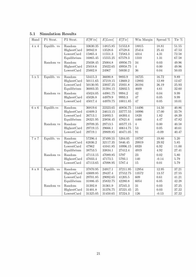
5.1 Simulation Results

Hand P1 Strat. P2 Strat. E[Win] E[Loss] E[Tie] Win Margin Spread % Tie %

4 x 4 Equilib. vs Random 33630.35 14815.85 51553.8 18815 18.81 51.55HighestCard 38942.8 13528.6 47528.6 25414 25.41 47.53LowestCard 15865.4 11551.3 72583.3 4314 4.31 72.58Equilibrium 16865.45 15555.25 67579.3 1310 1.31 67.58

Random vs Random 25038.45 25004.8 49956.75 34 0.03 49.96HighestCard 25018.6 25022.65 49958.75 4 0.00 49.96LowestCard 25002.8 24967 50030.2 36 0.04 50.03

5 x 5 Equilib. vs Random 53415.3 36690.8 9893.9 16725 16.72 9.89HighestCard 50111.65 37219.15 12669.2 12893 12.89 12.67LowestCard 50130.95 23937.25 25931.8 26194 26.19 25.93Equilibrium 36003.35 31394.15 32602.5 4609 4.61 32.60

Random vs Random 45024.05 44981.75 9994.2 42 0.04 9.99HighestCard 45026.8 44979.9 9993.3 47 0.05 9.99LowestCard 45017.4 44970.75 10011.85 47 0.05 10.01

6 x 6 Equilib.vs Random 36819.6 22323.65 40856.75 14496 14.50 40.86HighestCard 41609.3 24613.15 33777.55 16996 17.00 33.78LowestCard 26713.1 24893.5 48393.4 1820 1.82 48.39Equilibrium 28321.95 23856.45 47821.6 4466 4.47 47.82

Random vs Random 29709.35 29713.5 40577.15 4 0.00 40.58HighestCard 29719.15 29666.1 40614.75 53 0.05 40.61LowestCard 29719.1 29809.85 40471.05 91 -0.09 40.47

7 x 7 Equilib. vs Random 57296.4 37499.55 5204.05 19797 19.80 5.20HighestCard 62036.2 32117.35 5846.45 29919 29.92 5.85LowestCard 47962 41041.85 10996.15 6920 6.92 11.00Equilibrium 38753.5 33834.1 27412.4 4919 4.92 27.41

Random vs Random 47113.15 47089.85 5797 23 0.02 5.80HighestCard 47033.4 47173.5 5793.1 140 -0.14 5.79LowestCard 47113.65 47098.95 5787.4 15 0.01 5.79

8 x 8 Equilib. vs Random 37870.95 24917.1 37211.95 12954 12.95 37.21HighestCard 43009.85 29437.4 27552.75 13572 13.57 27.55LowestCard 29701.85 29092.65 41205.5 609 0.61 41.21Equilibrium 31886.45 25832.75 42280.8 6054 6.05 42.28

Random vs Random 31392.8 31361.9 37245.3 31 0.03 37.25HighestCard 31401.8 31376.75 37221.45 25 0.03 37.22LowestCard 31325.05 31450.65 37224.3 126 -0.13 37.22

21

5.2 Discussion of Results

Some interesting observations from the empirical results are discussed next. First,

note the sharp difference between the number of ties (Tie %) that result in games where

players start with an even number of cards (“even” games), and games where players

start with an odd number of cards (“odd” games). The number of ties is significantly

lower for “odd” games. Intuitively, this makes sense because it is only possible to tie

in an “odd” game if the last trick is a tie. In all other cases, all ties are resolved, and

there is a clear winner. Therefore, the probability that a particular game ends in a tie

is strongly influenced by the parity, odd or even, of the number of cards with which the

players start the game.

Further, the equilibrium strategy seems to do better against all other strategies for

the “odd” games as compared to the “even” games. For example, compare the equi-

librium versus lowest card strategy for the 5 x 5 and the 6 x 6 cases. Note that while

the number of losses is approximately the same for the two cases, the number of wins

is significantly lower for the 6 x 6 case. In other words, increasing the initial hand size

by 1, and changing its parity, causes a large number of wins for the equilibrium strategy

to turn into ties. This observation is strongly influenced by the observation discussed in

the previous paragraph.

We can also see that the “lowest card” strategy is a relatively good deterministic

strategy, if the opponent is playing either a random or an equilibrium strategy. While

the equilibrium strategy always defeats the “lowest card” strategy in an expected sense,

the difference between the number of wins and the number of losses is much less for

Equilibrium vs. Lowest Card, as compared to, for example, Equilibrium vs. Highest

Card, or Equilibrium vs. Random. Note that the optimal strategy against “lowest card”

would be “second lowest card”, where the player would play his second lowest card at

each trick and hence beat lowest card at every iteration of the entire game.

Conversely, “highest card” performs particularly badly against the equilibrium strat-

egy. Examining the vector of probabilities for the equilibrium strategy at the root node

suggests that “highest” card should have poor performance. The linear program puts no

weight on the highest card on the first trick for each of the 4 x 4 to 8 x 8 cases. In fact,

for the 7 x7 case, the highest two cards have a probability of zero at the top level. This

22

means that the highest cards should NEVER be played at the start of the game. The

“highest card” strategy does exactly what the linear program suggests it should not do.

Hence, its poor performance is not a surprise.

6 Potential Extensions

The theoretical framework and the associated computational system developed in

this paper are able to completely solve the game of jujitsu. From a computational stand-

point, there is not much more that can be done to extend this project.

From a theoretical standpoint, there is potentially work that can be done to gener-

alize and codify the conclusions drawn from analyzing the empirical results. Analyzing

different objective functions, that optimize on alternative parameters, is also an area

that can be explored.

7 Conclusion

We are exploring the opportunity of working with Dr. Kannan, our advisor, towards

a publication based on the work we have done for this project.

23

8 References

Arnold, K. The Java Programming Language

Binmore, Ken. Fun and Games: A Text on Game Theory

Devore, Jay. Probability and Statistics for Engineering and the Sciences

Kernighan and Ritchie. The C Programming Language

Kreyszig. Advanced Engineering Mathematics

Luce, Duncan. Games and Decisions: Introduction and Critical Survey

Various Readings on Linear Programming

Matlab Online Resources

Latex Online Resources

24