Equilibrium Phase Diagrams...Pressure-Temperature diagram: general case phase diagram of water...
49
-1- Equilibrium Phase Diagrams - Training course - M.-N. de NOIRFONTAINE, LSI, CNRS-CEA-Ecole Polytechnique, France [email protected] C. GIROD LABIANCA, CNRS-CTG Italcementi Group, France [email protected] G. INDEN, Max-Planck-Institut für Eisenforschung GmbH, Germany [email protected] MATGEN-IV Cargese, Corsica, France September 27, 2007
Transcript of Equilibrium Phase Diagrams...Pressure-Temperature diagram: general case phase diagram of water...

-1-
Equilibrium Phase Diagrams- Training course -
M.-N. de NOIRFONTAINE, LSI, CNRS-CEA-Ecole Polytechnique, [email protected]
C. GIROD LABIANCA, CNRS-CTG Italcementi Group, [email protected]
G. INDEN, Max-Planck-Institut für Eisenforschung GmbH, [email protected]
MATGEN-IVCargese, Corsica, France
September 27, 2007

-2-
Contents
1. Basic Thermodynamics1.1. Definition and experimental determination of an equilibrium phase diagram1.2. Thermodynamic study of phase diagrams and minimisation of the Gibbs free energy
From the Gibbs free energy variations of the phases, G(X,T), to the determination of the phase diagram (X: Composition, T: Temperature)
2. Introduction to “CALPHAD” formalismCALPHAD = CALculation of PHase Diagrams
From experimental data to G(X,T) thermodynamic polynomial functions
3. Introduction to the Thermo-Calc software. Demonstrations and examples
2.1. Thermodynamical models for solutions and compounds → G(X,T)2.2. Refinements of the model parameters based on selected experimental datasets
3.1. Thermo-Calc software = CALPHAD formalism + Thermodynamic databases of G(X,T)Calculation of phase equilibria by Gibbs energy minimisation process
3.2. Demonstrations and working examples: Two cases (Cu-Ni and Fe-Cr systems)

-3-
What is an equilibrium phase diagram?
Definition and experimental determination of an equilibrium phase diagram1.1.
• Graphical representation of the lines of equilibrium or phase boundaries: lines that demarcate where phase transitions occur
A: Triple pointsp, mp, nbp: sublimation, melting, normal boiling points
phase diagram of waterPressure-Temperature diagram: general case
A
Single (pure) substance: Pressure-temperature diagramTriple point: the unique intersection of the lines of equilibrium
between three states of matter, usually solid, liquid, and gas

-4-
Two-component or Binary phase diagrams: Temperature-composition diagram, P constant
Composition (concentration): Mole or mass fraction (or percent) of a constituent i in a given alloy
- Liquidus: the line above which the alloy is properly in a liquid (L) state - Solidus: the line below which the alloy is properly in a solid (α) state- Solvus: the line which represents the limit of solid solubility of a phase
Binary phase diagram of Pb-SnTemperature-composition diagram
Definition and experimental determination of an equilibrium phase diagram1.1.
XA = nA / N
- nA and nB : number of moles of A and B; mA and mB mass of A and B;- N = nA + nB: total mole number ; M = mA + mB: total mass;
XA and XB mole fractions of A and B: XB = nB / N
wA = mA / MwA and wB mass fractions of A and B:CA and CB mass percents wB = mB / M
Tem
pera
ture
Composition
Tem
pera
ture
Composition
XA + XB = 1
wA + wB = 1

-5-
Experimental determination of a phase diagramThermal analysis techniques
• T = f (t) cooling curves measurements for several compositionsPure compound: Fusion/Solidification or allotropic transition ↔ solidification at 1 transition temperatureBinary solution: Fusion/Solidification ↔ solidification in a range of temperature
liquidus and solidus
Definition and experimental determination of an equilibrium phase diagram1.1.
TmA
TmB
XB=1/4 XB=3/4
Temperature = f(composition)Temperature = f(time)
Tem
pera
ture
XB=0 XB=1/4 XB=3/4 XB=1
time
Plateau oftemperature
Range oftemperature
Liquidus (l)Solidus (s)
Tl
Tl
TS
TS
• More advanced techniques: DSC / DTA (Differential Scanning calorimetry / Thermal Analysis)
A
l l ll→α
α + l
α + l
l→α
B

-6-
dG = VdP - SdT
dG = VdP - SdT + Σµidni
Gibbs free energy
Thermodynamic study of phase diagrams. Minimisation of the Gibbs free energy1.2.
First law of thermodynamics: conservation of the energy in any processIntroduction of the internal energy EIntroduction of the enthalpy function H = E + PV and dH = dE + PdV + VdP
Second law of thermodynamicsIntroduction of the entropy function S and dS = dQ/T
Third law of thermodynamicsIntroduction of the Gibbs free energy function: G = H – TS = E + PV –TSAnd dG = dH – SdT – TdS = dE + PdV + VdP -SdT -TdS
Closed system: dE = dW + dQ = -PdV + TdS
Open system: dE = dW + dQ + Σµidni = -PdV + TdS + Σµidni
i ii T,P,nj
dGµ Gdn
⎛ ⎞= = ⎜ ⎟
⎝ ⎠
chemical energy contribution
chemical potential of component i, orpartial molar Gibbs free energy

-7-
Molar Gibbs energy and chemical potentials
= Σ i in µG
im i i iG x G x= Σ = Σ μ
Am AG G= = μ
Thermodynamic study of phase diagrams. Minimisation of the Gibbs free energy1.2.
• The molar Gibbs free energy Gm = Gibbs free energy of one mole of the substance
The chemical potential of this component is identical to its molar Gibbs free energy
• The Gibbs free energy G of a system is the sum of the chemical potentials of its constituents
One-component (A) system: XA=1
Xi molar fraction of component i
T,P constant
Binary system (A and B): XA and XB varying with XA+XB=1
A Bm A B A A B BG x G x G x x= + = μ + μ
T,P constant

-8-
Equilibrium criteria (1/2)
Thermodynamic study of phase diagrams. Minimisation of the Gibbs free energy1.2.
- Spontaneous transformation ↔ decrease of Gibbs free energy of the system - Equilibrium condition: dG = 0 ↔ Gibbs free energy of the system is minimum
A AG Gα β=
A AG Gα β<
Closed system. One-component (A) system
- At equilibrium ↔
If a substance A may be either in the α or β structure (phase) associated to Gα and Gβ
The stable structure is that which corresponds to the lowest Gibbs free energy of the system
- α more stable than β ↔
α and β coexist

-9-
Equilibrium criteria (2/2)
Thermodynamic study of phase diagrams. Minimisation of the Gibbs free energy1.2.
Open system. Two component or Binary system (1 and 2) or (A and B)
at equilibrium, dG = 0 ⇒
Considering: two phases α and β at equilibrium respectively associated to Gα and Gβ
µ1α = µ1
β and µ2α = µ2
β
dGα = µ1α dn1
α + µ2α dn2
α
dGβ = µ1β dn1
β + µ2β dn2
βT,P constant
total free energy change of the system: dG = dGα + dGβ
As the total amount of 1 and 2 are constant → dn1α = - dn1
β and dn2α = - dn2
β
dG = µ1α dn1
α + µ2α dn2
α - µ1β dn1
α - µ2β dn2
α
dG = (µ1α − µ1
β) dn1α + (µ2
α - µ2β ) dn2
α
for each component, equality of the chemical potentials in all phases (no chemical transfer)
As dn1α and dn2
α are independent,

-10-
- Pure compounds: melting points (Tm) determinations
A
AlG
G (T)(T)
α
A AA lm GGT α↔ =
α: solid phasel: liquid phase
AmTConsidering pure compound A (XB=0): How to determine its melting temperature ?
Thermodynamic study of phase diagrams. Minimisation of the Gibbs free energy1.2.
AmT ?
Tem
pera
ture
Temperature
Mol
ar G
ibbs
ene
rgy
GA
AAlG <Gα
XA=1, XB=0AAlG =Gα
AlAG <Gα
Mercier et al.

-11-
- Binary systems: determinations of the liquidus, solidus and solvus
leX
Thermodynamic study of phase diagrams. Minimisation of the Gibbs free energy1.2.
Chemical potentials and common tangent construction (1/4)
• Equilibrium phases and equilibrium compositions
Considering a binary system A-B: α (Gα) and β (Gβ ) two solid phases and l (Gl) liquid phaseFor each temperature, the common tangent between Gα and Gl or between Gα and Gβ give the compositions of the two phases in equilibrium:
eXα
(a) α and β not in equilibrium (b) α and β in equilibrium
The intercepts of the two axes by the tangent of the Gibbs free energy curve of the α phase at the composition X2
α
represent µ1α and µ2
α
Graphical representations of the chemical potentials of the two components by the method of intercepts:
Idem for the β phase
Equilibrium condition:
⇔ Common tangent
µ1α = µ1
β and µ2α = µ2
β
Solidus
• Liquidus, solidus and solvus determinations
T,P constant
Mol
ar G
ibbs
ene
rgy
A B A B
Lupis
Considering Gα or Gβ, and Gl
eXβeXα
eXβ
SolvusSolvus
Considering Gα and Gβ
orLiquidus

-12-
- Binary systems: determinations of the liquidus and solidus
lmG (X,T)
• Gap of miscibility in the solid state2 phases α: solid ↔
l: liquid ↔1 phase, α: solid
Chemical potentials and common tangent construction (2/4)
• Total miscibility of A and B
T<TcPhase demixing
Thermodynamic study of phase diagrams. Minimisation of the Gibbs free energy1.2.
mG (X,T)αmG (X,T)α
AG (X,T)α
AG (X,T)α
mmlG <Gα
BBlG =Gα
AAlG =Gα
XB=1
XA=1
mmlG >Gα
Mercier et al.
liquidussolidus solvus
α1 and α2: same crystal structure
“Isomorphous”

-13-
• Eutectic point: 3 phases, α and β two solid phases and l liquid phase
Thermodynamic study of phase diagrams. Minimisation of the Gibbs free energy1.2.
liquidus solidus
Chemical potentials and common tangent construction (3/4)- Binary systems: determinations of the liquidus and solidus
Mercier et al.Lupis
solvus
α and β: different crystal structures

-14-
- Binary systems: determinations of the liquidus and solidus
• Eutectic point: 2 phases, α solid phase and l liquid phase
Thermodynamic study of phase diagrams. Minimisation of the Gibbs free energy1.2.
Chemical potentials and common tangent construction (4/4)
α1 and α2: same crystal structures
“Eutectic”
Lupis

-15-
Conclusion
• First step: in the studied range of temperature and composition, it is absolutely necessary to have a preliminary knowledge of- the nature of the several phases:
solid solutions,defined compounds
- the possible presence of miscibility gap- and for each phase, the description of Gm(X,T)
• Second step: minimisation of the Gibbs free energyDetermination of the different boundaries lines (solvus, solidus and liquidus)by searching the equilibrium conditions.
for a binary system with two phases in equilibriumequilibrium condition ↔ searching for the two components the equality of the chemical potentials
Graphical method ⇔ comment tangent constructionCalculation method ⇔ Gibbs energy minimisation process
How to calculate a binary phase diagram?
Thermodynamic study of phase diagrams. Minimisation of the Gibbs free energy1.2.
Part 2
Part 3

-16-
Contents
1. Basic Thermodynamics1.1. Definition and experimental determination of an equilibrium phase diagram1.2. Thermodynamic study of phase diagrams and minimisation of the Gibbs free energy
From the Gibbs free energy variations of the phases, G(X,T), to the determination of the phase diagram (X: Composition, T: Temperature)
2. Introduction to “CALPHAD” formalismCALPHAD = CALculation of PHase Diagrams
From experimental data to G(X,T) thermodynamic polynomial functions
2.1. Thermodynamical models for solutions and compounds → G(X,T)2.2. Refinements of the model parameters based on selected experimental datasets
3. Introduction to the Thermo-Calc software. Demonstrations and examples
3.1. Thermo-Calc software = CALPHAD formalism + Thermodynamic databases of G(X,T)Calculation of phase equilibria by Gibbs energy minimisation process
3.2. Demonstrations and working examples: Two cases

-17-
- Pure species or stoichiometric compounds
Thermodynamic models for solutions and compounds 2.1.
nSER n
m m n2
G (T) H a bT cT ln T d T− = + + + ∑
Polynomial function for the Gibbs energy:
Form used by the Scientific Group ThermoData Europe (SGTE):
Gibbs energy relative to a standard element reference state (SER), where HmSER is the
enthalpy of the element or substance in its defined reference state at 298,15K2
P 2P
GC TT
∂= −
∂with
and the physical hypothesis of a linear variation of Cp:G = a + bT + cTlnT + dT2 ↔ Cp= -c – 2dT
The other terms are probably added in order to have a better refinement with theexperimental data

-18-
- Binary mixtures. Determination of the free energy change due to mixing
( )mixrefidealG G
om i i i e i
i iG x .G R.T. x .Log x= +∑ ∑
14243 144424443
emix
A BS klog W kln(N!/n !n !)= =mix
A e A B e BS R(x log (x ) x log (x ))= − +
Thermodynamic models for solutions and compounds 2.1.
• No chemical interaction between A and B
AA, BB and AB energy bonds are supposed identical → Hmix= 0
Random mixing of atoms → configurational entropy Smix
mix mix mixi e i
iG H TS RT x log (x )= − = ∑
{
ref
free energy changedue to mixingpure components
in their reference statesG
pure mix mixm i i
i iG G G x G G°= + = +∑ ∑
14243
?
A and B are quasi-identical atoms (1/3) Ideal model
(k: Boltzamm’s constant and W number of configurations)
(using Stirling’s approximation)

-19-
Thermodynamic models for solutions and compounds 2.1.
AB bond energies are different from the AA and BB bond energies
→ Hmix
→ Introduction of a parameter (LAB) for each pair of constituents, called interaction energy
• Interaction independent of the composition
Model based on the Braggs Williams approach
Random mixing of the atoms → configurational entropy
- Binary mixtures. Determination of the free energy change due to mixing
ij ij ijL A B .T ...
• Chemical interaction between A and B (pairwise interactions)
= + +
( )mixref mixideal excessG G G
om i i i e i i j ij
i i i j iG x .G R.T. x .Log x x .x .L
>= + +∑ ∑ ∑∑14243 144424443 1442443
mixmixref excessidealG G G Gm + +=
with Lij depending or not of T
A and B are quasi-identical atoms (2/3) Non Ideal or excess models of Redlish-KisterRegular solution
?
mixexcessH 0= ≠
mixexcessS 0=
mixidealS=
Mixing entropy whose source is supposed entirely configurational

-20-
- Binary mixtures. Determination of the free energy change due to mixing
( ) ( ) ( )ij ij ijL A B .T ...ν ν ν= + +
Thermodynamic models for solutions and compounds 2.1.
( ) ( ) ( )ij
mixref mixidéal excessG G G
Redlich-Kister polynom: L
om i i i e i i j i jij
i i i j iG x .G R.T. x .Log x x .x . L . x x
νν
> ν= + + −∑ ∑ ∑∑ ∑
6447448
14243 144424443 1444442444443
Excess model of Redlish-Kister model: generalisation
ν=0 ↔ Regular solution: Lij depending of the temperatureν=1 ↔ Non or sub-regular solution: Lij depending also of the temperature and the composition
( )mixref mixidéal excessG G G
o i jm i i i e i i j ij i ij j
i i i j iG x .G R.T. x .Log x x .x .(L .x L .x )
>= + + +∑ ∑ ∑∑14243 144424443 14444244443
• Chemical interaction between A and B dependent of the composition
A and B are quasi-identical atoms (2/3) Non Ideal or excess models of Redlich KisterNon or Sub-Regular solution

-21-
- Binary mixtures. Determination of the free energy change due to mixing
Thermodynamic models for solutions and compounds 2.1.
A and C are not quasi-identical atoms Sublattice model
• A and C can not mix: we consider two sublattices (A):(C)In each sublattice (s), various quasi-identical atoms can mix, such as: - (A,B):(C) or (A,B):(C,D) or (A,B…):(Va,C,D…) (Va, vacancy)- (A,B…)u:(Va,C,D)v
∑∑
−=
s
sva
ss
si
s
i yN
yNx
)1(
sinsVanSN
Introduction of the site fractionss
si
i
si
sva
sis
i Nn
nnn
y =+
=∑
total number of sites in sublattice s
number of moles of component i on sublattice snumber of vacancies on sublattice s
⇔
site fraction of component i on sublattice ssiy
( ) ( ) ( )ref
mix mixideal excessG
G T.S G H
so s s s s s s sm i j i:j i e i i j i jij
i j s i s i j imix mixideal excess
G y .y .G R.T. u y .Log y y .y . L . y y
=− =
νν
> ν= + + −∑∑ ∑ ∑ ∑∑∑ ∑
144442444431442443 144444424444443
In each sublattice: random mixing of the atoms → conf. entropy
In each sublattice, chemical interaction: ideal or excess modelmixS
with site fraction associated to the sublattice ss s su n /N=

-22-
SOLID PHASES. Solid solutions
Thermodynamic models for solutions and compounds 2.1.
Common models for solutions phases for the composition dependence:
• A and B are quasi-idendical:- Regular Solution Model – Excess model of Redlich-Kister (Redlich-Kister 1948)
• A and B are different:- Sublattice Model or the so-called Compound Energy Model(Sundman and Agren 1981; Andersson 1986; Hillert 2001)
LIQUID PHASES.
Ex: Cu-Ni: sub-regular solution Ex: Fe-Cr: regular solution
• The most common used model: Excess model of Redlish-Kister
• Other models developed in more specified cases
Ex: for oxide liquids (short-distance order )
- Two-Sublattice Ionic Liquid Model (Hillert 1985; Sundman 1991)- Associate Model (Sommer 1982)- Kapoor-Frohberg-Gaye Cell Model (Gay 1984)- Quasi-Chemical Model of ionic liquid (Pelton 1986)

-23-
Refinement strategy
Refinements of the model parameters based on selected experimental data2.2.
2. A thermodynamic model is chosen for each unknown phase of the diagram.This defines a set of of unknown model parameters (interaction parameters L)
1. Polynomial functions of the end members are always supposed well known.All the phases of the diagram must be known
3. A critical set of thermodynamic datafrom literature data or experimental measurements
is chosen for each unknown phase
4. Refinements (least-square method) of the model parameters on the thermodynamic data and equilibrium calculations
G(x,T) thermodynamic polynomial function → database

-24-
Contents
1. Basic Thermodynamics1.1. Definition and experimental determination of an equilibrium phase diagram1.2. Thermodynamic study of phase diagrams and minimisation of the Gibbs free energy
From the Gibbs free energy variations of the phases, G(X,T), to the determination of the phase diagram (X: Composition, T: Temperature)
2. Introduction to “CALPHAD” formalismCALPHAD = CALculation of PHase Diagrams
From experimental data to G(X,T) thermodynamic polynomial functions
3. Introduction to the Thermo-Calc software. Demonstrations and examples
2.1. Thermodynamical models for solutions and compounds → G(X,T)2.2. Refinements of the model parameters based on selected experimental datasets
3.1. Thermo-Calc software = CALPHAD formalism + Thermodynamic databases of G(X,T)Calculation of phase equilibria by Gibbs energy minimisation process
3.2. Demonstrations and working examples: Two cases

-25-
Thermo-Calc software
Thermo-Calc software = CALPHAD formalism + Thermodynamic databases of G(X,T)3.1.
THERMODYNAMICDATABASES
G(X,T)
CALPHADformalism+
Thermo-Calcsofware
2. Second case:All the phases of the diagram ARE NOT in the database.
Assessment of the phase diagram by the refinement strategy
1. First case:All the phases of the diagrams ARE in the database.
Calculation of the phase diagram by energy minimisation process
Examples: Cu-Ni, Fe-Cr

-26-
Structure of the Thermo-Calc software: the 6 basic modules in daily use
Thermo-Calc software = CALPHAD formalism + Thermodynamic databases of G(X,T)3.1.
SYS
TDB
POLY
TAB
POST
GES
System Utilities
Thermodynamic DataBase: thermodynamic data retrieval
Gibbs Energy System: thermodynamic phase descriptions (models)
Tabulation: tabulate thermodynamic functions
Equilibrium Calculation
Post-Processor: plotting phase diagrams

-27-
Cu-Ni: Total miscibility in the solid and liquid states
mT 1085 C(1358K)= °⎯⎯⎯⎯⎯⎯⎯⎯→
Demonstrations and working examples: First case3.2.
Features of the experimental known phase diagram
Total miscibility of Cu and Ni in the liquid L
Total miscibility of Cu and Ni in the solid phase α
Coexistence of the two phases α and L
Pure Cu: α (fcc) liquidPure Ni: α (fcc) mT 1455 C(1728K)= °⎯⎯⎯⎯⎯⎯⎯⎯→ liquid
Cu-Ni. Experimental phase diagram between above 1000°C
Liquid
α(fcc) solid solution (Cu,Ni)Liquid + α(fcc)
Miscibility gap: α1+α2(magnetic ordering)
Cu Ni
595K(322°C)
Pure Cu - Mixture: total miscibility - Pure Ni%Ni

-28-
Cu-Ni: Total miscibility in the solid and liquid statesDescription of the phases in the database. Models and values of the parameters (1/3)
Demonstrations and working examples: First case3.2.
Which thermodynamic database?“SSOL2” which contains Cu and Ni elements and the two phases Liquid phase: “Liquid”
α(fcc) phase: “FCC_A1”
Which models are used?Liquid: Excess model of Redlish Kister. Non-regular solution
( ) ( )liq liq 1 1m Cu Cu Ni Ni Cu e Cu Ni e Ni Cu Ni CuNi CuNi Cu NiG x .G x .G R.T.(x .Log x x .Log x ) x .x (L L (x x ) )°= + + + + + −
FCC_A1: Solid solutionSublattice model: 1st sublattice with Cu and Ni, 2nd sublattice with vacancy: Cu,Ni:Va
cf. the annexe document EXAMPLE 1Calculation of the Cu-Ni phase diagram between 1000 and 1600°CExercice 1: SELECTING THE THERMODYNAMIC FUNCTIONS (TDB and GES modules)
How can I extract the values of the thermodynamic parameters ?Handle the TDB and GES modules
Thermo-Calc exercise
( ) ( )Cu Ni Cu Cu Ni Ni Cu Ni Cu Ni
1 fcc 1 fcc 1 1 1 1 1 1 1 1 1 1m Cu:Va Ni:Va e e CuNi CuNiG y .G y .G R.T.(y .Log y y .Log y ) y .y (L L (y y ) )°= + + + + + −

-29-
Description of the phases in the database. Models and values of the parameters (2/3)
Demonstrations and working examples: First case3.2.
Liquid: Excess model of Redlish Kister. Non-regular solution
( ) ( )liq liq 1 1m Cu Cu Ni Ni Cu e Cu Ni e Ni Cu Ni CuNi CuNi Cu NiG x .G x .G R.T.(x .Log x x .Log x ) x .x (L L (x x ) )°= + + + + + −

-30-
( ) ( )Cu Ni Cu Cu Ni Ni Cu Ni Cu Ni
1 fcc 1 fcc 1 1 1 1 1 1 1 1 1 1m Cu:Va Ni:Va e e CuNi CuNiG y .G y .G R.T.(y .Log y y .Log y ) y .y (L L (y y ) )°= + + + + + −
FCC_A1: Solid solutionSublattice model: 1st sublattice with Cu and Ni, 2nd sublattice with vacancy: (Cu,Ni):(Va)
Description of the phases in the database. Models and values of the parameters (3/3)
Magnetic contribution terms
Demonstrations and working examples: First case3.2.
are not useful in our studied range of T
1yVa =↔

-31-
Cu-Ni: Total miscibility in the solid and liquid states
cf. the annexe documentEXAMPLE 1Calculation of the Cu-Ni phase diagram between 1000 and 1600°CExercise 2. CALCULATING AND PLOTTING THE PHASE DIAGRAM (POLY and POST modules)
Plotting the calculated phase diagram (1/2)
Demonstrations and working examples: First case3.2.
Calculate and plot by yourself the phase diagramHandle the POLY and POST modules
Thermo-Calc exercise

-32-
Cu-Ni: Total miscibility in the solid and liquid states
Experimental phase diagram Calculated phase diagram
Demonstrations and working examples: First case3.2.
Comparison of the experimental and the calculated phase diagrams
1000
1100
1200
1300
1400
1500
1600
TEM
PER
ATU
RE_
CEL
SIU
S
0 10 20 30 40 50 60 70 80 90 100MASS_PERCENT NI
THERMO-CALC (2007.09.06:16.34) : DATABASE:SSOL2 N=1, P=1.01325E5;
LIQUID
FCC_A1
LIQUID+FCC_A1
Plotting the calculated phase diagram (2/2)

-33-
Plotting the thermodynamic functions: Molar Gibbs energy curves (1/2)
Demonstrations and working examples: First case3.2.
Cu-Ni: Total miscibility in the solid and liquid states
cf. the annexe documentEXAMPLE 1Calculation of the Cu-Ni phase diagram between 1000 and 1600°CExercise 3. PLOTTING THE MOLAR GIBBS ENERGY CURVES G=f(X)
Plot by yourself the molar Gibbs energy curvesHandle the POLY and POST modules
Thermo-Calc exercise
-86
-85
-84
-83
-82
-81
-80
-79
-78
-77
103
GM
(*)
0 0.1 0.2 0.3 0.4 0.5 0.6 0.7 0.8 0.9 1.0
MOLE_FRACTION NI
THERMO-CALC (2007.09.06:19.22) : DATABASE:SSOL2 N=1, P=1.01325E5, T=1473;
1
1:X(NI),GM(LIQUID)
2
2:X(NI),GM(FCC_A1)
12

-34-
1000
1100
1200
1300
1400
1500
1600
TEM
PER
ATU
RE_
CEL
SIU
S0 0.1 0.2 0.3 0.4 0.5 0.6 0.7 0.8 0.9 1.0
MOLE_FRACTION NI
THERMO-CALC (2007.09.07:12.05) : DATABASE:SSOL2 N=1, P=1.01325E5;
LIQUID
FCC_A1
LIQUID+FCC_A1
-99
-98
-97
-96
-95
-94
-93
-92
-91
-90
103
GM
(*)
0 0.1 0.2 0.3 0.4 0.5 0.6 0.7 0.8 0.9 1.0
MOLE_FRACTION NI
THERMO-CALC (2007.09.06:19.25) : DATABASE:SSOL2 N=1, P=1.01325E5, T=1623;
1
1:X(NI),GM(LIQUID)
2
2:X(NI),GM(FCC_A1)
1
2
-86
-85
-84
-83
-82
-81
-80
-79
-78
-77
103
GM
(*)
0 0.1 0.2 0.3 0.4 0.5 0.6 0.7 0.8 0.9 1.0
MOLE_FRACTION NI
THERMO-CALC (2007.09.06:19.22) : DATABASE:SSOL2 N=1, P=1.01325E5, T=1473;
1
1:X(NI),GM(LIQUID)
2
2:X(NI),GM(FCC_A1)
12
-90
-89
-88
-87
-86
-85
-84
-83
-82
-81
103
GM
(*)
0 0.1 0.2 0.3 0.4 0.5 0.6 0.7 0.8 0.9 1.0
MOLE_FRACTION NI
THERMO-CALC (2007.09.06:19.25) : DATABASE:SSOL2 N=1, P=1.01325E5, T=1523;
1
1:X(NI),GM(LIQUID)
2
2:X(NI),GM(FCC_A1)
1
2
Plotting the thermodynamic functions (2/2)
T=1473K=1200°C T=1523K=1250°C T=1623K=1350°C
T=1473K=1200°CT=1523K=1250°C
T=1623K=1350°C

-35-
Fe-Cr: how to handle a miscibility gap
mT 912 C(1185K)= °⎯⎯⎯⎯⎯⎯⎯⎯→
mT 1394 C(1667K)= °⎯⎯⎯⎯⎯⎯⎯⎯→
Demonstrations and working examples: Second case3.2.
mT 912 C(1185K)= °⎯⎯⎯⎯⎯⎯⎯⎯→Pure Fe: α (cc) liquidPure Cr: α (fcc) mT 1800 C(2073K)= °⎯⎯⎯⎯⎯⎯⎯⎯→ liquid
γ (cfc) δ (cc) mT 1535 C(1808K)= °⎯⎯⎯⎯⎯⎯⎯⎯→
σ intermediate phase (brittle phase)
α solid solution in Fe-α or Fe-δ: “ferrite”
γ solid solution in Fe-γ: “austenite”
Cr → “alphagene” element
Total miscibility in liquid
Miscibility gap in the solid state
Features of the experimental known phase diagram
α or δ (cc)γ (fcc)
Fe
austenite loop
duplex loop
Barralis et al.
Azeotrope-type phase diagram

-36-
Fe-Cr: how to handle a miscibility gapDescription of the phases in the database. Models and values of the parameters (1/5)
Demonstrations and working examples: Second case3.2.
Which thermodynamic database?
Which models are used?
How to see the values of the thermodynamic parameters ?Handle the TDB and GES modules
Thermo-Calc exercise
cf. the annexe documentEXAMPLE 2Calculation of the Fe-Cr phase diagram between 600 and 2200°CExercice 1. SELECTING THE THERMODYNAMIC FUNCTIONS (TDB and GIBBS modules)
Liquid phase: “Liquid”γ (fcc) phase: “FCC_A1”α (cc) phase: “BCC_A2”σ sigma phase: “SIGMA”
Which thermodynamic database?“PTERN” which contains Fe and Cr elements and the four phases
Liquid: Excess model of Redlish Kister: Regular solution
FCC_A1: Solid solutionSublattice model: 1st sublattice with Fe and Cr, 2nd sublattice with vacancy: (Fe,Cr):(Va)
BCC_A2: Solid solutionSublattice model: 1st sublattice with Fe and Cr, 2nd sublattice with vacancy: (Fe,Cr):(Va)
SIGMA: Solid solutionSublattice model: 1st sublattice with Fe, 2nd sublattice with Cr, 3rd sublattice with Fe and Cr: (Fe):(Cr):(Fe,Cr)

-37-
Description of the phases in the database. Models and values of the parameters (2/5)
Demonstrations and working examples: Second case3.2.
Liquid: Excess model of Redlish Kister: Regular solution
( ) ( )liq liqm Cr Cr Fe Fe Cr e Cr Fe e Fe Cr Fe CrFeG x .G x .G R.T.(x .Log x x .Log x ) x .x L°= + + + +

-38-
( ) ( )1 fcc 1 fcc 1 1 1 1 1 1 1 1 1 1m Cr Cr:Va Fe Fe:Va Cr e Cr Fe e Fe Cr Fe CrFe CrFe Cr FeG y .G y .G R.T.(y .Log y y .Log y ) y .y (L L (y y ) )°= + + + + + −
Description of the phases in the database. Models and values of the parameters (3/5)
Demonstrations and working examples: Second case3.2.
FCC_A1: Solid solutionSublattice model: 1st sublattice with Cr and Fe, 2nd sublattice with vacancy: (Cr,Fe):(Va)
Magnetic contribution termsare not useful in our studied range of T
1yVa =↔
-39-
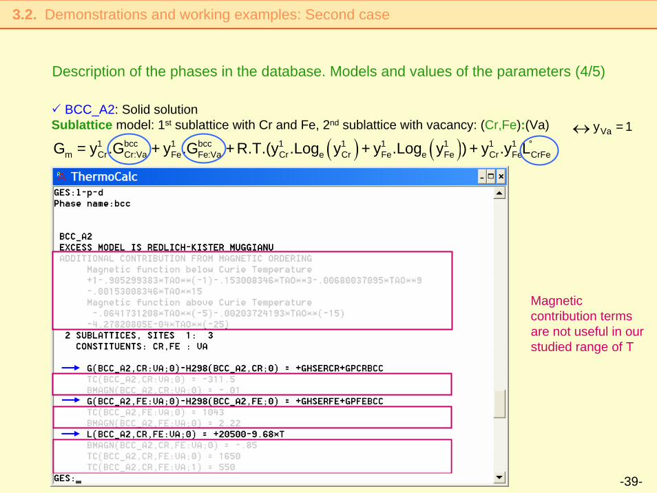
Description of the phases in the database. Models and values of the parameters (4/5)
Demonstrations and working examples: Second case3.2.
BCC_A2: Solid solutionSublattice model: 1st sublattice with Cr and Fe, 2nd sublattice with vacancy: (Cr,Fe):(Va)
Magnetic contribution termsare not useful in our studied range of T
( ) ( )1 bcc 1 bcc 1 1 1 1 1 1 °m Cr Cr:Va Fe Fe:Va Cr e Cr Fe e Fe Cr Fe CrFeG = y .G + y .G +R.T.(y .Log y + y .Log y ) + y .y L
Vay = 1↔

-40-
Description of the phases in the database. Models and values of the parameters (5/5)
Demonstrations and working examples: Second case3.2.
SIGMA: Solid solutionSublattice model: 1st sublattice with Fe, 2nd sublattice with Cr, 3rd sublattice with Fe and Cr: (Fe)8:(Cr)4:(Cr,Fe)18
( ) ( )Fe Cr Cr Fe Fe
3 3 3 3 3 3m Cr Fe:Cr:Cr Fe:Cr:Fe e eG y .G y .G R.T.(18(y .Log y y .Log y ))= + + +
1 2Fe Cry = y = 1↔

-41-
Fe-Cr: how to handle a miscibility gap
Calculate and plot by yourself the phase diagramHandle the POLY and POST modules
Thermo-Calc exercise
cf. the annexe documentEXAMPLE 2Calculation of the Fe-Cr phase diagram between 600 and 2200°CExercice 2. CALCULATING AND PLOTTING THE PHASE DIAGRAM (POLY and POST modules)
Plotting the calculated phase diagram (1/2)
Demonstrations and working examples: Second case3.2.

-42-
Comparison of the experimental and the calculated phase diagrams
Plotting the calculated phase diagram (2/2)
Experimental phase diagram Calculated phase diagram
Fe-Cr: how to handle a miscibility gap
600
800
1000
1200
1400
1600
1800
2000
TEM
PER
ATU
RE_
CEL
SIU
S
0 10 20 30 40 50 60 70 80 90 100
MASS_PERCENT CR
THERMO-CALC (2007.09.12:20.23) : DATABASE:PTERN N=1, P=1.01325E5;
FCC_A1BCC_A2
LIQUID
LIQUID+BCC_A2
SIGMA BCC_A2+SIGMA
BCC_A2+FCC_A1
Demonstrations and working examples: Second case3.2.

-43-
References
1) Andersson, J.-O., Fernandez Guillermet, A., Hillert, M., Jansson, B., and Sundman, B. (1986), "A compound-energy model of ordering in a phase with sites of different coordination numbers", Acta Metall., 34(3), 437-445.2) Barralis, J., Maeder, G., and Trotignon, J.-P. (2005), "Précis de Métallurgie". AFNOR/Nathan, Paris.3) Callister, W.D. (2001), "Science et génie des matériaux". 782 p, Mont-Royal (Quebec).4) Gaye, H., and Welfringer, J. (1984) Modelling of the thermodynamic properties of complex metallurgical slags. Metallurgical slags and fluxes, 2nd Int. Symp., p. 357-375, Warrendale.5) Guillet, L. (1964), "Diagrammes de phases en métallurgie". 144 p. Masson, Paris.6) Hillert, M., Jansson, B., Sundman, B., and Agren, J. (1985), "A two-sublattice model for molten solutions withdifferent tendency for ionization", Metall. Trans. A, 16, 261-266.7) Hillert, M. (2001), "The compound energy formalism", J. of Alloys and Compounds, 320, 161-176.8) Lupis, C.H.P. (1983), "Chemical Thermodynamics of Materials". 581 p. Elsevier Science Publishing, New-York.9) Mercier, J.-P., Zambelli, G., and Kurz, W. (1999), "Traité des Matériaux, Vol.1". 500 p. Presses Polytechniques et universitaires romandes, Lausanne.10) Pelton, A.D., and Blander, M. (1986), "Thermodynamic Analysis of Ordered Liquid Solutions by a ModifiedQuasichemical Approach - Application to the Silicate Slags", Metall. Trans. B, 17, 805-815.11) Redlich, O., and Kister, A.T. (1948), "Algebraic representation of thermodynamic properties and theclassification of solutions", Ind. Eng. Chem., 40(2), 345-348.12) Saunders, N., and Miodownik, A.P. (1998), "CALPHAD (Calculation of the Phase Diagrams): A comprehensiveGuide". 480 p. Pergamon materials series, Oxford.13) Sundman, B. (1991), "Modification of the two-sublattice model for liquids", Calphad, 15(2), 109-119.14) Sommer, F. (1982), "Association Model for the Description of the Thermodynamic Functions of Liquid Alloys", Z. Metallkd., 73(2), 72-76.15) Sundman, B., and Agren, J. (1981), "A regular solution model for phases with several components andsublattices, suitable for computer applications", J. Phys. Chem. Solids, 42, 297-301.

-44-
Thermo-Calc information
-45-
SUPPLEMENTS

-46-
Microstructure and phase diagram
Definition and experimental determination of an equilibrium phase diagram1.1.
Exemple: Pb-Sn phase diagram
Composition and proportion of the phases during the cooling of an liquid alloy
Variation of the composition of the phases during the cooling Proportion of the phases
“Level Rule”
fα = (CL-C0) / (CL – Cα) = MQ / PQ
P M Q
fL = (C0-Cα) / (CL – Cα) = PM / PQ
C0: mass percent (%wt) of Sn in the alloyCα: mass percent (%wt) of Sn in α phaseCL: mass percent (%wt) of Sn in L phasefα : mass percent (%) of the α phasefL : mass percent (%) of the L phase
Cα CL
For an alloy of concentration C0
→ Sn (%wt)
fα + fl = 1fαCα + fLCL = C0
C0
Callister

-47-
Gibbs Phase Rule
V = C + n – φC: number of system componentsn: number of variables which can vary (temperature, pressure, volume) φ: maximum number of stable phases
Variance (V) or number of degrees of freedom: number of independent variables
Binary system: - 2 components → C = 2 and V = 2 + n – φ- 1 variable, neglecting pressure and volume variations: P fixed (P=1 atm) → n = 1
V = 3 – φ
One-component system:- 1 component → C = 1 - varying variables: temperature and pressure → n = 2
V = 3 – φ
φ=3 ↔ V=0 → P,T fixed ⇒ At most three coexisting phases for one single (P,T) couple (see triple point)
φ=3 ↔ V=0 → T fixed ⇒ At most three coexisting phases for one single TEcalled eutectic or peritectic temperature
Definition and experimental determination of an equilibrium phase diagram1.1.
Invariant equilibrium ↔ V=0: equilibrium attained only for a single set of values
-48-
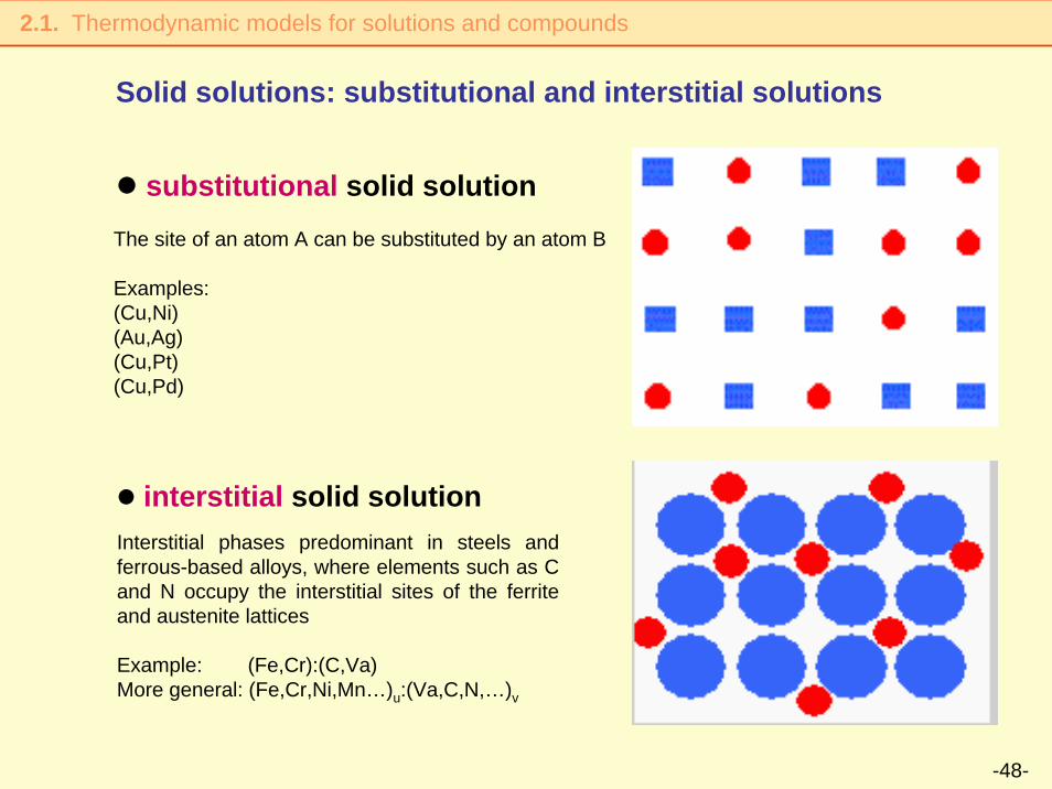
Solid solutions: substitutional and interstitial solutions
Thermodynamic models for solutions and compounds 2.1.
substitutional solid solution
interstitial solid solution
The site of an atom A can be substituted by an atom B
Examples: (Cu,Ni)(Au,Ag)(Cu,Pt)(Cu,Pd)
Interstitial phases predominant in steels and ferrous-based alloys, where elements such as C and N occupy the interstitial sites of the ferrite and austenite lattices
Example: (Fe,Cr):(C,Va)More general: (Fe,Cr,Ni,Mn…)u:(Va,C,N,…)v

-49-
Conversions and constants
• Avogadro’s number: N=6.022 1023 mol-1
• Boltzmann’s constant: k=1,3806 J/K
• Gaz constant: R=8.314 J/K mol = 1.987 cal/K mol
• G(cal) = G(J) / 4.184
• T(K) = T(°C) + 273.15
• 1 inche = 2,5 cm
• 1 cm = 0,4 inche