Equilibrium Conditions and Linearization in …mettler/Courses/AEM 5333 (spring 2013)/AEM5333... ·...

Equilibrium Conditions and

Linearization in Simulink

Gary Balas

Aerospace Engineering and Mechanics

February 28, 2011

http://www.aem.umn.edu/courses/aem5495.

Ultrastick Nonlinear Simulation: UAV_trim

Ultrastick Nonlinear Simulation

The UAV Model for Linearization is a masked block containing

the Ultrastick 6DOF EOM, Forces and Moments, Auxiliary Equations and Environment equations. Selecting Look Under Mask function for the UAV Model for Linearization block displays these subsystems.

Ultrastick Nonlinear Simulation

Each subsystem 6DOF EOM (masked), Forces and Moments, Auxiliary

Equations and Environment contains additional subsystems. The layout of your Simulink diagram is critical its maintainability, readability, verification and validation. It is important to spend the time laying out your model prior to building it.

Simulink Bus Creator

Simulink blocks that can improve the layout and maintainability of your

model.

Bus Creator

• The Bus Creator block combines a set of signals into a bus. To bundle a group of

signals with a Bus Creator block, set the block's Number of inputs parameter to

the number of signals in the group.

• The Bus Creator block assigns a name to each signal on the bus that it creates.

This allows you to refer to signals by name when searching for their sources.

Simulink Bus Creator cont’d

• Change the name of any signal by editing its name on the block diagram or in the

Signal Properties dialog box.

Simulink Bus Selector

Bus Selector

• The Bus Selector block outputs a specified subset of the elements of the bus at its input. The block can output the specified elements as separate

signals or as a new bus

• Caution It is not recommended to use Bus Selector blocks in library blocks, because such use complicates changing the library blocks and increases

the likelihood of errors. .

Operating Points in Simulink Control Design Tlbx

The Ultrastick nonlinear model provides a high fidelity representation of the radio

controlled plane. Linear models of the vehicle are used for control design. A

linear model is generated from small perturbations around an equilibrium

condition. The Simulink Control Design (SCD) toolbox functions findop is

used to find an equilibrium point.

• A Simulink full model operating point includes information from all of the blocks in a

Simulink model. When you use the Simulink Control Design GUI or the MATLAB

command line to create operating points for a model, you are actually creating an operating point object (what is referred to as the operating point). The operating point is

a subset of the Simulink full-model operating point. SCD differentiates between block to

determine if they are included in the operating point object.

– Blocks with double value states, root level inports with double data type (YES)

– Root level inport blocks with nondouble or complex data type (NO)

– Blocks with internal state representation that impacts blocks output, e.g. memory (NO)

– Source blocks with outputs specified by block dialog parameers, e.g. Constant (NO)

• Note that the operating point consists of values for all the states in the model, although

only those states between the linearization points are linearized. The whole model contributes to the operating point values of the states, inputs, and outputs of the portion

of the model you are linearizing.

Ultrastick Nonlinear Simulation: UAV_trim

Creating Operating Points

We will focus on command line tools to specify and calculate operating points with SCD.

• Initial values and constraints for the inputs and states.

• Exact values for inputs and states

• Time/Event to extract operating point during simulation.

operspec – Operating Point Object

operspec is used when only some values of constraints of the operating point are known exactly. operspec creates an operating point specification object for

the model>>

Operating Specification for the Model UAV_NL.

(Time-Varying Components Evaluated at time t=0)

States:

----------

(1.) UAV_NL/Nonlinear UAV Model/6DoF EOM/Calculate DCM & Euler Angles/phi theta psi

spec: dx = 0, initial guess: 0.00481


spec: dx = 0, initial guess: 0

(2.) UAV_NL/Nonlinear UAV Model/6DoF EOM/p,q,r

spec: dx = 0, initial guess: 5.8e-025

spec: dx = 0, initial guess: -1.88e-023


(3.) UAV_NL/Nonlinear UAV Model/6DoF EOM/ub,vb,wb




(4.) UAV_NL/Nonlinear UAV Model/Auxiliary Equations/xe,ye,ze

spec: dx = 0, initial guess: 4.05e-016


spec: dx = 0, initial guess: -100

(5.) UAV_NL/Nonlinear UAV Model/Forces and Moments/Electric Propulsion Forces and Moments/Engine speed Integrator


Creating Operating Points, cont’dInputs:

----------

(1.) UAV_NL/elevator

initial guess: 0

(2.) UAV_NL/aileron

initial guess: 0

(3.) UAV_NL/rudder

initial guess: 0

(4.) UAV_NL/throttle

initial guess: 0

(5.) UAV_NL/flap

initial guess: 0

Outputs:

----------

(1.) UAV_NL/V_s spec: none

(2.) UAV_NL/beta spec: none

(3.) UAV_NL/alpha spec: none

(4.) UAV_NL/h spec: none

(5.) UAV_NL/phi spec: none

(6.) UAV_NL/theta spec: none

(7.) UAV_NL/psi spec: none

(8.) UAV_NL/p spec: none

(9.) UAV_NL/q spec: none

(10.) UAV_NL/r spec: none

(11.) UAV_NL/gamma spec: none

Creating Operating Points, cont’d

The operating point specification object contains objects for all the states, inputs, and

outputs in the model. By typing the object's name at the command line you can see a formatted display of key object properties. Alternatively the get command can be used

to list all the properties of the object.

>> getop.State(3))

Block: 'UAV_NL/Nonlinear UAV Model/6DoF EOM/ub,vb,wb'

StateName: ''

x: [3x1 double]

Nx: 3

Ts: [0 0]

SampleType: 'CSTATE'

inReferencedModel: 0

Known: [3x1 logical]

SteadyState: [3x1 logical]

Min: [3x1 double]

Max: [3x1 double]

Description: ''

To set the 3rd vector states, velocities u, v, and w, to have a known forward velocity, u = 17 m/s, and leaving v and w to be unknown, first change Known to 1 for u and the others set to 0.

% u, v, w -- Body velocities

op.States(3).Known = [1; 0; 0];

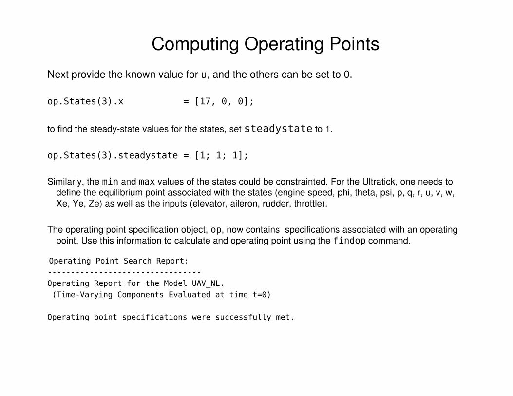
Computing Operating Points

Next provide the known value for u, and the others can be set to 0.

op.States(3).x = [17, 0, 0];

to find the steady-state values for the states, set steadystate to 1.

op.States(3).steadystate = [1; 1; 1];

Similarly, the min and max values of the states could be constrainted. For the Ultratick, one needs to define the equilibrium point associated with the states (engine speed, phi, theta, psi, p, q, r, u, v, w, Xe, Ye, Ze) as well as the inputs (elevator, aileron, rudder, throttle).

The operating point specification object, op, now contains specifications associated with an operating point. Use this information to calculate and operating point using the findop command.

Operating Point Search Report:

---------------------------------

Operating Report for the Model UAV_NL.

(Time-Varying Components Evaluated at time t=0)

Operating point specifications were successfully met.

Computing Operating Points, cont’d

States:

----------

(1.) UAV_NL/Nonlinear UAV Model/6DoF EOM/Calculate DCM & Euler Angles/phi theta psi

x: 0.00481 dx: -1.72e-026 (0)

x: 0.0217 dx: -1.87e-023 (0)

x: 0 dx: -2.75e-023 (0)

(2.) UAV_NL/Nonlinear UAV Model/6DoF EOM/p,q,r

x: 5.8e-025 dx: 9e-012 (0)

x: -1.88e-023 dx: 7.75e-022 (0)

x: -2.74e-023 dx: 7.77e-013 (0)

(3.) UAV_NL/Nonlinear UAV Model/6DoF EOM/ub,vb,wb

x: 17 dx: 2.96e-011 (0)

x: -2.92e-021 dx: -2.92e-017 (0)

x: 0.37 dx: -3.2e-022 (0)

(4.) UAV_NL/Nonlinear UAV Model/Auxiliary Equations/xe,ye,ze

x: 4.05e-016 dx: 17

x: -3.82e-015 dx: -0.00178

x: -100 dx: 0

(5.) UAV_NL/Nonlinear UAV Model/Forces and Moments/Electric Propulsion Forces and Moments/Engine speed Integrator

x: 827 dx: -3.01e-010 (0)

Computing Operating Points, cont’dInputs:

----------

(1.) UAV_NL/elevator u: 0.091 [-0.436 0.436]

(2.) UAV_NL/aileron u: 0.0218 [-0.436 0.436]

(3.) UAV_NL/rudder u: -0.0086 [-0.436 0.436]

(4.) UAV_NL/throttle u: 0.571 [0 1]

(5.) UAV_NL/flap u: 0 [-0.436 0.436]

Outputs:

----------

(1.) UAV_NL/V_s y: 17 [-Inf Inf]

(2.) UAV_NL/beta y: -1.72e-022 [-Inf Inf]

(3.) UAV_NL/alpha y: 0.0217 [-Inf Inf]

(4.) UAV_NL/h y: 79.1 [-Inf Inf]

(5.) UAV_NL/phi y: 0.00481 [-Inf Inf]

(6.) UAV_NL/theta y: 0.0217 [-Inf Inf]

(7.) UAV_NL/psi y: 0 [-Inf Inf]

(8.) UAV_NL/p y: 5.8e-025 [-Inf Inf]

(9.) UAV_NL/q y: -1.88e-023 [-Inf Inf]

(10.) UAV_NL/r y: -2.74e-023 [-Inf Inf]

(11.) UAV_NL/gamma y: 0 [-Inf Inf]

The operating point search report, rep, is also generated. The x or u values give the state or input values. The dx values give the time derivatives of each state, with desired dx values in parentheses. The fact that the dx values are near zero indicates that the operating point is at steady state.

Linearization using SCD

Prior to linearizing the Simulink model of your system, configure it by choosing

linearization input and output points. SCD requires you to

1.Store linearization points in an input/output (I/O) object.

2.Edit the I/O object, when necessary, such as when computing the open-loop model.

3.The input and output points define the portion of your model being linearized. Setting the

OpenLoop property of a linearization point to 'on' allows you to compute an open-loop

model.

An easy way define the inputs and outputs of your model is through the use of inports and

outports. Alternatively, an I/O object can be used to define inputs and outputs to the

model using the linio function. The call to linio is

IO=LINIO('blockname',PORTNUM,TYPE,OPENLOOP)

'blockname� corresponds to the block whose signal is of interest, PORTNUM is the outport number of blockname, TYPE is input/output type, e.g. �in�, �out�, and OPENLOOP provides for the loop to be broken. For UAV_trim, the inputs to the Ultrastick

are the surfaces and throttle and the outputs of interest are the states and navigation data.

Linearization using SCD

ultraio(1)=linio('UAV_trim/Bus Creator',1,'in');

ultraio(2)=linio('UAV_trim/Sum',1,'in')

ultraio(3)=linio('UAV_trim/UAV Model for Linearization',1,'out');

ultraio(4)=linio('UAV_trim/UAV Model for Linearization',2,'out')

Linearization IOs:

--------------------------

Block UAV_trim/Bus Creator, Port 1 is marked with the following properties:

- No Loop Opening

- An Input Perturbation

- No signal name. Linearization will use the block name

Block UAV_trim/Sum, Port 1 is marked with the following properties:

- No Loop Opening

- An Input Perturbation

- A signal name: throttle

Block UAV_trim/UAV Model for Linearization, Port 1 is marked with the following properties:

- An Output Measurement

- No Loop Opening


Block UAV_trim/UAV Model for Linearization, Port 2 is marked with the following properties:

- An Output Measurement

- No Loop Opening


Linearization of UAV_trim

Given a defined operating point, gsop, and input/output description, ultraio, a linearized

model of the nonlinear Ultrastick model can be derived. Note that the resulting linear model has 44 outputs, which is due to the bus outputs of UAV Model for Linearization.

olp = linearize('UAV_NL’,OperatingPoint.op_point);size(olp)

State-space model with 11outputs, 5 inputs, and 13 states.

olp.StateName

ans =

'\phi'

'\theta'

'\psi'

'p'

'q'

'r'

'u'

'v'

'w'

'Xe'

'Ye'

'Ze'

'\omega'

Linearization of UAV_trim

An alternative is to define only output signals from the bus selectors, ultraio(1)=linio('UAV_NL/Control Inputs',1,'in');

ultraio(2)=linio('UAV_NL/States',1,'in');



olp = linearize('UAV_NL',ultraio,ysop);

size(olp)

State-space model with 3 outputs, 5 inputs, and 13 states.

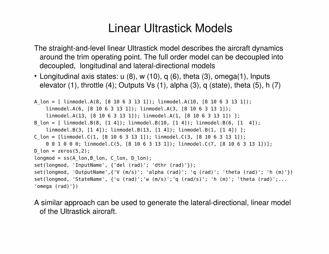
Linear Ultrastick Models

The straight-and-level linear Ultrastick model describes the aircraft dynamics around the trim operating point. The full order model can be decoupled into decoupled, longitudinal and lateral-directional models

• Longitudinal axis states: u (8), w (10), q (6), theta (3), omega(1), Inputs elevator (1), throttle (4); Outputs Vs (1), alpha (3), q (state), theta (5), h (7)

A_lon = [ linmodel.A(8, [8 10 6 3 13 1]); linmodel.A(10, [8 10 6 3 13 1]);

linmodel.A(6, [8 10 6 3 13 1]); linmodel.A(3, [8 10 6 3 13 1]);

linmodel.A(13, [8 10 6 3 13 1]); linmodel.A(1, [8 10 6 3 13 1]) ];

B_lon = [ linmodel.B(8, [1 4]); linmodel.B(10, [1 4]); linmodel.B(6, [1 4]);

linmodel.B(3, [1 4]); linmodel.B(13, [1 4]); linmodel.B(1, [1 4]) ];

C_lon = [linmodel.C(1, [8 10 6 3 13 1]); linmodel.C(3, [8 10 6 3 13 1]);

0 0 1 0 0 0; linmodel.C(5, [8 10 6 3 13 1]); linmodel.C(7, [8 10 6 3 13 1])];

D_lon = zeros(5,2);

longmod = ss(A_lon,B_lon, C_lon, D_lon);

set(longmod, 'InputName', {'del (rad)'; 'dthr (rad)'});

set(longmod, 'OutputName',{'V (m/s)'; 'alpha (rad)'; 'q (rad)'; 'theta (rad)'; 'h (m)'})

set(longmod, 'StateName', {'u (rad)';'w (m/s)';'q (rad/s)'; 'h (m)'; 'theta (rad)';...

'omega (rad)'})

A similar approach can be used to generate the lateral-directional, linear model of the Ultrastick aircraft.

Assessment of SAS/CAS in Nonlinear Simulation

Upon defining the desire operating points through out the flight regime, linear

models are synthesized are each trim point. It is important to compare these

models to understand the change in vehicle dynamics as a function of flight

condition. The following strategy

• Define operating points through out the flight regime

• Generate linear models at operating points

• Compare dynamic response of the linear models across the flight regime.

• Synthesize a stability augmentation system (SAS) and control augmentation

system (CAS) for the longitudinal and lateral-direction axes.

• Given a fixed, linear SAS and CAS for the flight envelope, access the

performance and robustness of the SAS and CAS on the linear models.

Assessment of SAS/CAS in Nonlinear Simulation

Once the linear assessment of the controllers is acceptable, the SAS/CAS

performance and robustness should be assessed on full nonlinear aircraft

simulation.

• Integrate SAS/CAS in nonlinear simulation.

• Define initial condition for states and inputs for comparison with linear

responses.

• Assess performance and robustness in nonlinear simulation

• Perform Monte Carlo assessment of performance and robustness by varying

parameters and models based on engineering insight.

Ultrastick with SAS/CAS

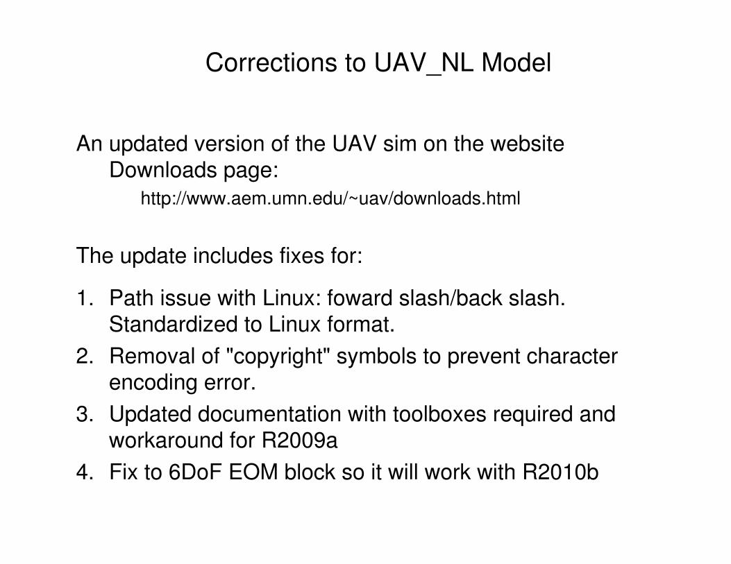
Corrections to UAV_NL Model

An updated version of the UAV sim on the website Downloads page:

http://www.aem.umn.edu/~uav/downloads.html

The update includes fixes for:

1. Path issue with Linux: foward slash/back slash. Standardized to Linux format.

2. Removal of "copyright" symbols to prevent character encoding error.

3. Updated documentation with toolboxes required and workaround for R2009a

4. Fix to 6DoF EOM block so it will work with R2010b

Equilibrium Conditions and Linearization in …mettler/Courses/AEM 5333 (spring 2013)/AEM5333... ·...

Documents

Transcript of Equilibrium Conditions and Linearization in …mettler/Courses/AEM 5333 (spring 2013)/AEM5333... ·...