Sensors 2012, 12, 4074-4090; doi:10.3390/s120404074OPEN ACCESS

sensorsISSN 1424-8220

www.mdpi.com/journal/sensors

Article

Equations for Solar TrackingAlexis Merlaud 1,?, Martine De Maziere 1, Christian Hermans 1 and Alain Cornet 2

1 Belgian Institute for Space Aeronomy, Avenue Circulaire 3, 1180 Brussels, Belgium;E-Mails: martine@aeronomie.be (M.D.M.); christh@oma.be (C.H.)

2 Institute of Condensed Matter and Nanosciences, UCL, Chemin du Cyclotron 2, 1348Louvain-La-Neuve, Belgium; E-Mail: alain.cornet@uclouvain.be

? Author to whom correspondence should be addressed; E-Mail: alexis.merlaud@aeronomie.be;Tel.: +32-2-373-03-82; Fax: +32-2-374-84-23.

Received: 9 February 2012; in revised form: 16 March 2012 / Accepted: 16 March 2012 /Published: 27 March 2012

Abstract: Direct sunlight absorption by trace gases can be used to quantify them andinvestigate atmospheric chemistry. In such experiments, the main optical apparatus is oftena grating or a Fourier transform spectrometer. A solar tracker based on motorized rotatingmirrors is commonly used to direct the light along the spectrometer axis, correcting for theapparent rotation of the Sun. Calculating the Sun azimuth and altitude for a given time andlocation can be achieved with high accuracy but different sources of angular offsets appearin practice when positioning the mirrors. A feedback on the motors, using a light positionsensor close to the spectrometer, is almost always needed. This paper aims to gather themain geometrical formulas necessary for the use of a widely used kind of solar tracker,based on two 45◦ mirrors in altazimuthal set-up with a light sensor on the spectrometer, andto illustrate them with a tracker developed by our group for atmospheric research.

Keywords: solar tracker; Fourier transform infrared spectrometry; algorithms

Classification: PACS 42.68.Wt;92.60.hd;92.60.hf;42.68.Ay

1. Introduction

Spectroscopic analyses of direct incident sunlight are commonly used in atmospheric research.Such experiments make use of the Sun as a light source to quantify molecular absorptions in

Sensors 2012, 12 4075

the atmosphere and then retrieve trace gas abundances. Stratospheric ozone [1] and greenhousegases [2] are routinely measured with this technique from ground-based Fourier transform infrared(FTIR) spectrometers, e.g., within the Network for the Detection of Atmospheric Composition Change(NDACC, http://www.ndacc.org/). In the UV-visible range, light scattering is more important andenables spectroscopic studies of the atmosphere in other geometries such as zenith measurements [3].However, direct sunlight is also used [4,5], its unique and unambiguous light path making it advantageousfor some applications [6]. Beside the spectrometer, the main part of the involved apparatus in directsunlight spectrometry is the solar tracker, required to compensate for the Sun’s diurnal motion.

Several kinds of trackers, sometimes referred to as heliostats, are used for atmospheric spectrometry,based on setups of one or several rotating mirrors. Some of them are equatorially mounted, like in TableMountain Facility [4] or Harestua [7]. In this case, one rotational axis is parallel to the Earth’s axis. Itenables a high tracking accuracy without a computer, since only one axis has to be driven at the Earth’srotation speed. To our knowledge, it is the only setup working without feedback on the Sun’s position.On the other hand, equatorial mounts are large, need to be aligned accurately and their mechanical designis difficult. Most of the trackers used today are controlled by a computer enabling remote operation andautomation. The computer first calculates the Sun position, moves the mirrors to point to the Sun andthen controls these mirrors to optimize the signal on some kind of light sensor. For some trackers, thelight sensor is attached to the moving part, whether it is a single mirror [8] or a mount of two mirrors [9].Compared to the solution presented below, the retroaction is simplified. The drawback is that the trackingis done some meters away from the spectrometer and is thus less accurate and stable.

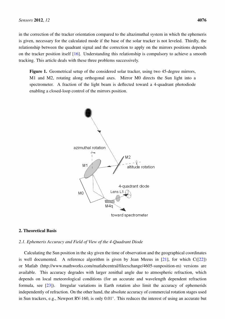
Figure 1 shows a popular altazimuthal tracker design. It consists of two elliptical mirrors held in45 degrees relative to the vertical, facing each other (M1 and M2). Both M1 and M2 rotate along theazimuthal axis and M2 rotates as well around a horizontal axis (altitude direction). M0, and possiblyother fixed mirrors, direct the light beam into the spectrometer optical axis. A 4-quadrant photodiode isused as a position sensor for a closed-loop control of the mirrors position once their positioning towardsthe Sun has been set with enough accuracy, i.e., once the Sun’s image is visible by the photodiode. Thisaltazimuthal setup is used with FTIR systems, e.g., in Kiruna [10] and Park Falls, Wisconsin [11]; ithas been installed in Harestua to replace the equatorially mounted system [12]. Compact versions havealso been developed for field campaigns [13,14]. A commercial version is sold by Bruker to be installedon their FTIR spectrometers [15]. A recent progress in the pointing accuracy has been reported [16],replacing the traditional quadrant diode with a CCD camera, but the problems discussed hereafter remainthe same.

Because developing a solar tracker is typically a master’s thesis work [10,13,14], technicalimplementations are difficult to access in the literature. Some more information is available aboutthe systems used in solar energy applications but their geometries differ [17–20]. Someone buildinga Sun tracker can quickly find ephemeris calculations in many programming languages, but other issuesarise quickly. It is first necessary to characterize the field-of-view (FOV) of the 4-quadrant diode inthe considered optical design. This serves two purposes: determining the accuracy needed for theephemeris’s algorithm and making sure this FOV is larger than the Sun’s apparent diameter (9 mrad).This last point is important to track constantly the center of the Sun, which reduces the uncertaintiesin the air mass factor and avoids Doppler shifts on the edges of the Sun ([16]). A second problem lies

Sensors 2012, 12 4076

in the correction of the tracker orientation compared to the altazimuthal system in which the ephemerisis given, necessary for the calculated mode if the base of the solar tracker is not leveled. Thirdly, therelationship between the quadrant signal and the correction to apply on the mirrors positions dependson the tracker position itself [16]. Understanding this relationship is compulsory to achieve a smoothtracking. This article deals with these three problems successively.

Figure 1. Geometrical setup of the considered solar tracker, using two 45-degree mirrors,M1 and M2, rotating along orthogonal axes. Mirror M0 directs the Sun light into aspectrometer. A fraction of the light beam is deflected toward a 4-quadrant photodiodeenabling a closed-loop control of the mirrors position.

2. Theoretical Basis

2.1. Ephemeris Accuracy and Field of View of the 4-Quadrant Diode

Calculating the Sun position in the sky given the time of observation and the geographical coordinatesis well documented. A reference algorithm is given by Jean Meeus in [21], for which C([22])or Matlab (http://www.mathworks.com/matlabcentral/fileexchange/4605-sunposition-m) versions areavailable. This accuracy degrades with larger zenithal angle due to atmospheric refraction, whichdepends on local meteorological conditions (for an accurate and wavelength dependent refractionformula, see [23]). Irregular variations in Earth rotation also limit the accuracy of ephemeridsindependently of refraction. On the other hand, the absolute accuracy of commercial rotation stages usedin Sun trackers, e.g., Newport RV-160, is only 0.01◦. This reduces the interest of using an accurate but

Sensors 2012, 12 4077

complex algorithm for ephemeris’s calculation, which is anyway not necessary providing a closed-loopcontrol is performed on the mirrors’ position. In this case, the lowest acceptable accuracy is thusdetermined by the field of view of the 4-quadrant diode: once the Sun image hits the quadrant, thetracking can be performed in closed-loop.

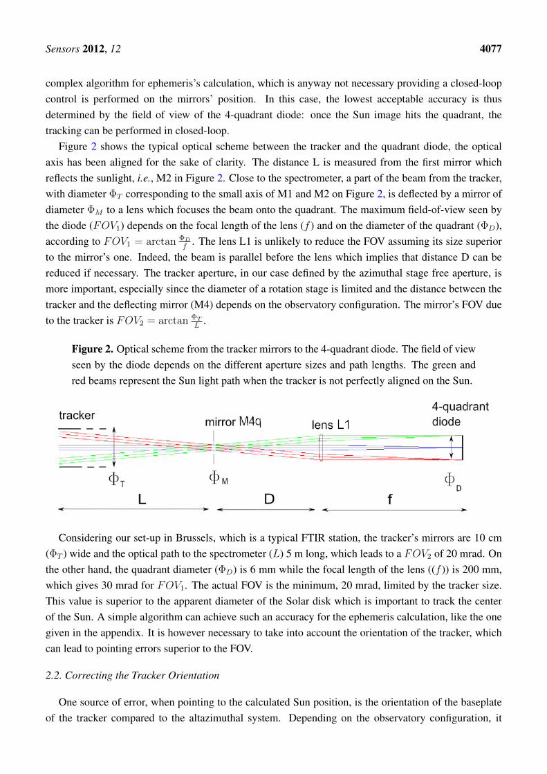
Figure 2 shows the typical optical scheme between the tracker and the quadrant diode, the opticalaxis has been aligned for the sake of clarity. The distance L is measured from the first mirror whichreflects the sunlight, i.e., M2 in Figure 2. Close to the spectrometer, a part of the beam from the tracker,with diameter ΦT corresponding to the small axis of M1 and M2 on Figure 2, is deflected by a mirror ofdiameter ΦM to a lens which focuses the beam onto the quadrant. The maximum field-of-view seen bythe diode (FOV1) depends on the focal length of the lens (f ) and on the diameter of the quadrant (ΦD),according to FOV1 = arctan ΦD

f. The lens L1 is unlikely to reduce the FOV assuming its size superior

to the mirror’s one. Indeed, the beam is parallel before the lens which implies that distance D can bereduced if necessary. The tracker aperture, in our case defined by the azimuthal stage free aperture, ismore important, especially since the diameter of a rotation stage is limited and the distance between thetracker and the deflecting mirror (M4) depends on the observatory configuration. The mirror’s FOV dueto the tracker is FOV2 = arctan ΦT

L.

Figure 2. Optical scheme from the tracker mirrors to the 4-quadrant diode. The field of viewseen by the diode depends on the different aperture sizes and path lengths. The green andred beams represent the Sun light path when the tracker is not perfectly aligned on the Sun.

Considering our set-up in Brussels, which is a typical FTIR station, the tracker’s mirrors are 10 cm(ΦT ) wide and the optical path to the spectrometer (L) 5 m long, which leads to a FOV2 of 20 mrad. Onthe other hand, the quadrant diameter (ΦD) is 6 mm while the focal length of the lens ((f )) is 200 mm,which gives 30 mrad for FOV1. The actual FOV is the minimum, 20 mrad, limited by the tracker size.This value is superior to the apparent diameter of the Solar disk which is important to track the centerof the Sun. A simple algorithm can achieve such an accuracy for the ephemeris calculation, like the onegiven in the appendix. It is however necessary to take into account the orientation of the tracker, whichcan lead to pointing errors superior to the FOV.

2.2. Correcting the Tracker Orientation

One source of error, when pointing to the calculated Sun position, is the orientation of the baseplateof the tracker compared to the altazimuthal system. Depending on the observatory configuration, it

Sensors 2012, 12 4078

may be difficult or impossible to align accurately the tracker along the North-South direction. If itwas the only problem, the remaining constant offset could be simply fitted and added in the calculatedazimuth. However, because the baseplate is never completely leveled either, other offsets are added to thecalculated positions, affecting both azimuth and elevation in a way that depends on the pointing directionof the tracker. Some tracker uses an active search method to solve this problem. In practice they reachthe calculated position and achieve spiral motion around this point to set the sun spot in the field-of-viewof the sensor. Misalignment effect can on the other hand be taken into account in the calculation requiresdetermining the Euler angles of the observatory and the tracker baseplate, respectively, compared to theazimuthal system. We discuss the Euler angles before describing our way to determine them. For thesake of simplicity, we only mention the observatory in the following, considering that the baseplate tobe part of it.

Figure 3. Illustration of the Euler Angles of an observatory compared to the altazimuthalcoordinate system.

Euler angles of an observatory may be seen, as in Figure 3, as consecutive rotations around threeorthogonal axes needed to account for the pitch, roll and yaw of this observatory. Converting the solaraltitude and azimuth to the observatory frame requires thus to compute the multiplication of three rotationmatrices along the different axes, i.e., Rx(γ), Ry(β) and Rz(α). The resulting matrix Moffset expressesthe transformation of coordinates due to the Euler angles.

Moffsets =

1 0 0

0 cos γ − sin γ

0 sin γ cos γ

× cos β 0 sin β

0 1 0

− sin β 0 cos β

×cosα − sinα 0

sinα cosα 0

0 0 1

(1)

Sensors 2012, 12 4079

The calculations leads to:

Moffsets =

cosα cos β − sinα cos β sin β

cosα sin β sin γ + sinα cos(γ) cosα cos γ − sinα sin β sin γ − cos β sin γ

sinα sin γ − cosα sin β cos γ cosα sin γ + sinα sin β cos γ cos β cos γ

(2)

In Cartesian coordinates, the unit vector (xt,yt,zt) giving the direction of the Sun in the observatoryframe will thus be related to the solar spherical coordinates(az0,alt0) in the altazimuthal system:xtyt

zt

= Moffsets ×

cos alt0 cos az0

cos alt0 sin az0

sin alt0

(3)

Substituting Moffset with Equation (2) we get the following expressions for those coordinates:

xt = cos (α + az0) cos β cos alt0 + sin β sin alt0

yt = (cos (α + az0) sin β sin γ + sin (α + az0) cos γ) cos alt0

− cos β sin γ sin alt0

zt = (sin (α + az0) sin γ − cos (α + az0) sin β cos γ) cos alt0

+ cos β cos γ sin alt0

(4)

These new Cartesian coordinates can then be converted to altitude (altt) and azimuth (azt) anglesrelative to the tracker:

ρt =√x2t + y2

t

altt = atan2 (zt, ρt)

azt = atan2 (yt, xt)

(5)

In the above equation, atan2(y, x), available in many programming languages, stands for theargument of the complex number x + iy. It is closely related to the arctangent of y/x but it indicatesunambiguously the quadrant of this angle on the trigonometric circle.

Determining Euler angles accurately by measurements is not easy. An analytical method to estimatethem is given in [17] which basically consists of recording the position of the tracker at three differenttimes and solving Equation (4). This is appropriate for the studied case, i.e., a collector for solar energyapplication installed outside with only one mirror and no closed-loop control. With our consideredtwo-mirror tracker, which does not collect light but directs it toward a spectrometer, other sources ofmisalignments appear. Indeed, the tracker is also likely to be misaligned compared to the spectrometer,and mirror themselves can be tilted. Other angles can be considered in Moffsets and is done in [10].In practical applications, despite the three Euler angles, the calculated mode is likely able to reach theSun within the FOV of the 4-quadrant diode. With the closed-loop control it is easy to track the Sunduring a whole clear-sky day providing an operator correctly sets the Sun tracker initially. Euler anglescan then be fitted using all the recorded positions of the mirrors during the day. It has the advantage thatother sources of misalignment are included: even if only three angles are fitted which may not exactlybe the Euler angles, they minimize simultaneously the effects of all offsets. We implement this methodin Section 4. This requires the closed-loop control of the tracker on the Sun position.

Sensors 2012, 12 4080

2.3. Ray Tracing in the Tracker

The photodiode signal indicates that the Sun beam is tilted compared to the optical axis of thespectrometer. The photodiode signals must be converted into angular movements of the altitude andazimuth axes of the tracker to correct the misalignment. If the photodiode was placed on the referenceframe of the mirror M2 this conversion would be straightforward, but due to its position after the trackerit depends on the position of the tracker mirrors. A trial-and-error method to correct the misalignmentis theoretically possible using analogue electronics without a computer but a smoother tracking can beachieved if the conversion is understood.

The conversion can be expressed once again by a matrix, which transforms in this case a vectorhitting mirror M1 to a vector pointing to a direction in the sky given by its altitude and azimuth. It is theopposite of the light direction but is simpler to figure out, and considering Fermat principle, yields thesame information.

The rotation of the two motorized stages can be accounted for using rotation matrices as describedin the previous section. The reflection on the two mirrors is modeled using another matrix which takesthe form:

M = I − 2nnT (6)

where I is the identity matrix and n the normal vector to the mirror surface. At reference position, themirror are parallel and thus their normal is the same, given by the vector (0, 1√

2,− 1√

2). The transformation

matrix for the two mirror is thus the same, MR, which is, from Equation (6):

MR =

1 0 0

0 0 1

0 1 0

Figure 4 presents the tracker pointing to an azimuth θ1 and a zenith angle of θ2. The reference frames

<1 and <2 are respectively attached to the mirrors M1 and M2, with the x axes in the direction of theirsmall semi-axes and the y axes along the line joining the two mirrors. The optical system inside theframe, with only mirrors M1 and M2, can be expressed as a transformation whose matrix Mtracker is:

Mtracker = Rz(θ1)×Ry(θ2)×MR ×Ry(−θ2)×MR ×Rz(−θ1) (7)

The above formula is derived as follow: (a) the reflection on M2 (MR) is expressed in the referenceframe of <1 with a change of basis involving Ry(−θ2); (b) this product of three matrices is multiplied onits right side by the preceding (seen from the spectrometer) reflection on M1(MR); (c) another change ofbasis is performed to express the transformation in <0, involving Rz(−θ1). i.e.,

Mtracker =

cos θ1 − sin θ1 0

sin θ1 cos θ1 0

0 0 1

× cos θ2 0 sin θ2

0 1 0

− sin θ2 0 cos θ2

×1 0 0

0 0 1

0 1 0

×

cos θ2 0 − sin θ2

0 1 0

sin θ2 0 cos θ2

×1 0 0

0 0 1

0 1 0

× cos θ1 sin θ1 0

− sin θ1 cos θ1 0

0 0 1

(8)

Sensors 2012, 12 4081

Figure 4. The tracker mirrors and their rotation can be modeled as rotation matrices in theirreference frames, which apply to the beam vector. Note that the z and y axes are the samerespectively for (<0,<1) and (<1,<2).

Developing the matrix product yields the matrix of the tracker optical system as a function of thetracker position (θ1,θ2):

Mtracker=

cos θ1 cos θ2 cos(θ1 − θ2) + sin θ1 sin(θ1 − θ2) cos θ1 cos θ2 sin(θ1 − θ2)− sin θ1 cos(θ1 − θ2) cos θ1 sin θ2

sin θ1 cos θ2 cos(θ1 − θ2)− cos θ1 sin(θ1 − θ2) cos θ1 cos(θ1 − θ2) + sin θ1 cos θ2 sin(θ1 − θ2) sin θ1 sin θ2

− sin θ2 cos θ1 − θ2 − sin θ2 sin θ1 − θ2 cos θ2

The transformation expressed by Mtracker can now be applied to a vector corresponding to the Sun

light beam direction on the spectrometer side of the tracker. It will lead to the position of the Sun inCartesian coordinates. The vector is built from the 4 diode signals (VA,VB,VC,VD), as represented inFigure 5. Basically an offset position (ε1,ε2) is computed for the Sun spot on the diode plane comparedto its center by: ε1 = (VB + VC)− (VA + VD)

ε2 = (VA + VB)− (VC + VD)(9)

Sensors 2012, 12 4082

Figure 5. Sun spot hitting the quadrant, not to scale.

The spot offset (ε1,ε2) defines 2 coordinates of the beam vector. The last one, Λ, should representthe distance from the diode to mirror M1. Multiplying Mtracker by the quadrant vector (ε1,ε2,Λ) wouldyield accurate Sun angles after conversion to spherical coordinates, but is not practically possible with adiode, contrary to an imaging sensor. The calculated position (xs,ys,zs) hereafter is thus not absolute butis sufficient to get the sign of the rotations to apply on the axes. Λ can be chosen arbitrarily as long as itsabsolute value is large enough compared to ε1 and ε2. The solar pseudo-coordinates are then:xsys

zs

= Mtracker ×

ε1

ε2

Λ

(10)

In practice, the quadrant vector may differ from (ε1,ε2,Λ) due to reflections such as on the mirrors M0and M4q on Figure 1, necessary to deviate a part of the beam to the 4-quadrant photodiode. Defining theposition vector thus requires to pay attention to the optical path from M1 to the photodiode. In section 4,we explain how we deal with the problem in our particular case.

Developing Equation (10) yields:

xs = (cos θ1 cos θ2 sin (θ1 − θ2)− sin θ1 cos (θ1 − θ2))ε2

+ (sin θ1 sin (θ1 − θ2) + cos θ1 cos θ2 cos (θ1 − θ2))ε1 + Λ cos θ1 sin θ2

ys = (sin θ1 cos b sin (θ1 − θ2) + cos θ1 cos (θ1 − θ2))ε2

+ (sin θ1 cos θ2 cos (θ1 − θ2)− cos θ1 sin (θ1 − θ2))ε1 + Λ sin θ1 sin θ2

zs = − sin θ2 sin (θ1 − θ2)ε2 − sin θ2 cos (θ1 − θ2)ε1 + Λ cos θ2

(11)

It is then possible to calculate roughly an altitude(θ2S) and azimuth(θ1S) for the Sun applying theCartesian to spherical coordinates conversion (Equation (5)). This position is approximate and relative

Sensors 2012, 12 4083

to the tracker since it does not take into account the Euler angles described in the last section, but whatmatters are the signs of the differences between these calculated values and the current altitude andazimuth relative to the tracker, defined by θ1 and θ2. The angular corrections to apply on the two axesare then: dθ1 = sgn(θ1S − θ1)k1

dθ2 = sgn(θ2S − θ2)k2

(12)

where k1 and k2 are the tracking angle steps that should be small to have a smooth tracking, yet largeenough for the mechanical resolution of the rotation stages and the apparent movement of the Sun. Theazimuth changes for instance at a rate of 15◦ per hour, assuming 1 second between the steps, k1 shouldnot be under 0.004◦.

3. Automation Issues

From a control theory perspective, the altazimuthal tracker and its feedback is a non-linear multi-inputmulti-output (MIMO) system. Indeed, two outputs defining the pointing direction (θ1 and θ2 ) arecontrolled by two inputs, i.e., the coordinates of the Sun spot on the photodiode(ε1 and ε2), and therelationship between the inputs and the outputs varies with the position of the tracker. However, havingmodeled this relationship in the previous section, it is possible to change the feedback scheme whiletracking. In control theory, this is an example of adaptive control.

The correction of the azimuth and altitude angles discussed earlier only takes into account the currenterror, i.e., the tilt of the solar beam compared to the optical axis of the spectrometer. This is very coarseand can lead to oscillations. A proper feedback loop includes the derivative and integral of the errorrelative to the time as well, respectively to reduce the overshoot and the residual part of the errors. Thisinvolves to tune the three parameters of a proportional–integral–derivative (PID) controller. Consideringthe two outputs, the setup needs two PID controllers.

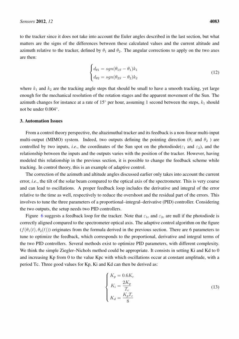
Figure 6 suggests a feedback loop for the tracker. Note that ε1c and ε2c are null if the photodiode iscorrectly aligned compared to the spectrometer optical axis. The adaptive control algorithm on the figure(f(θ1(t), θ2(t))) originates from the formula derived in the previous section. There are 6 parameters totune to optimize the feedback, which corresponds to the proportional, derivative and integral terms ofthe two PID controllers. Several methods exist to optimize PID parameters, with different complexity.We think the simple Ziegler–Nichols method could be appropriate. It consists in setting Ki and Kd to 0and increasing Kp from 0 to the value Kpc with which oscillations occur at constant amplitude, with aperiod Tc. Three good values for Kp, Ki and Kd can then be derived as:

Kp = 0.6Kc

Ki =2Kp

Tc

Kd =KpTc

8

(13)

Sensors 2012, 12 4084

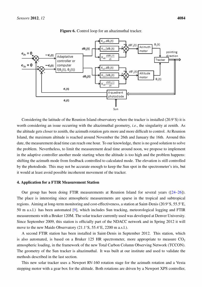
Figure 6. Control loop for an altazimuthal tracker.

Considering the latitude of the Reunion Island observatory where the tracker is installed (20.9◦S) it isworth considering an issue occurring with the altazimuthal geometry, i.e., the singularity at zenith. Asthe altitude gets closer to zenith, the azimuth rotation gets more and more difficult to control. At ReunionIsland, the maximum altitude is reached around November the 26th and January the 16th. Around thisdate, the measurement dead time can reach one hour. To our knowledge, there is no good solution to solvethe problem. Nevertheless, to limit the measurement dead time around noon, we propose to implementin the adaptive controller another mode starting when the altitude is too high and the problem happens:shifting the azimuth mode from feedback controlled to calculated mode. The elevation is still controlledby the photodiode. This may not be accurate enough to keep the Sun spot in the spectrometer’s iris, butit would at least avoid possible incoherent movement of the tracker.

4. Application for a FTIR Measurement Station

Our group has been doing FTIR measurements at Reunion Island for several years ([24–26]).The place is interesting since atmospheric measurements are sparse in the tropical and subtropicalregions. Aiming at long-term monitoring and cost-effectiveness, a station at Saint-Denis (20.9◦S, 55.5◦E,50 m a.s.l.) has been automated [9], which includes Sun tracking, meteorological logging and FTIRmeasurements with a Bruker 120M. The solar tracker currently used was developed at Denver University.Since September 2009, this station is officially part of the NDACC network and in Spring 2012 it willmove to the new Maido Observatory (21.1◦S, 55.4◦E, 2200 m a.s.l.).

A second FTIR station has been installed in Saint-Denis in September 2012. This station, whichis also automated, is based on a Bruker 125 HR spectrometer, more appropriate to measure CO2

atmospheric loading, in the framework of the new Total Carbon Column Observing Network (TCCON).The geometry of the Sun tracker is altazimuthal. It was built at our institute and used to validate themethods described in the last section.

This new solar tracker uses a Newport RV-160 rotation stage for the azimuth rotation and a Vextastepping motor with a gear box for the altitude. Both rotations are driven by a Newport XPS controller,

Sensors 2012, 12 4085

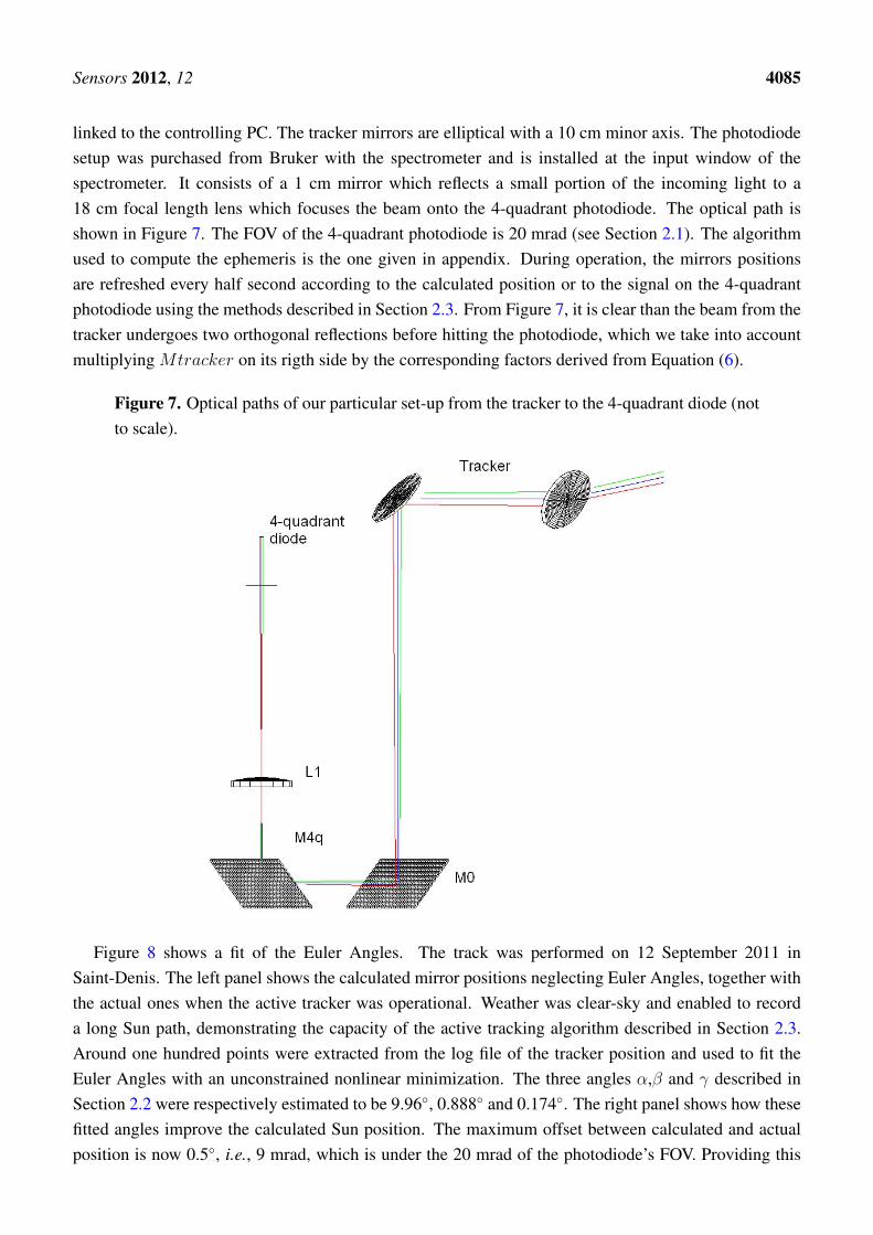
linked to the controlling PC. The tracker mirrors are elliptical with a 10 cm minor axis. The photodiodesetup was purchased from Bruker with the spectrometer and is installed at the input window of thespectrometer. It consists of a 1 cm mirror which reflects a small portion of the incoming light to a18 cm focal length lens which focuses the beam onto the 4-quadrant photodiode. The optical path isshown in Figure 7. The FOV of the 4-quadrant photodiode is 20 mrad (see Section 2.1). The algorithmused to compute the ephemeris is the one given in appendix. During operation, the mirrors positionsare refreshed every half second according to the calculated position or to the signal on the 4-quadrantphotodiode using the methods described in Section 2.3. From Figure 7, it is clear than the beam from thetracker undergoes two orthogonal reflections before hitting the photodiode, which we take into accountmultiplying Mtracker on its rigth side by the corresponding factors derived from Equation (6).

Figure 7. Optical paths of our particular set-up from the tracker to the 4-quadrant diode (notto scale).

Figure 8 shows a fit of the Euler Angles. The track was performed on 12 September 2011 inSaint-Denis. The left panel shows the calculated mirror positions neglecting Euler Angles, together withthe actual ones when the active tracker was operational. Weather was clear-sky and enabled to recorda long Sun path, demonstrating the capacity of the active tracking algorithm described in Section 2.3.Around one hundred points were extracted from the log file of the tracker position and used to fit theEuler Angles with an unconstrained nonlinear minimization. The three angles α,β and γ described inSection 2.2 were respectively estimated to be 9.96◦, 0.888◦ and 0.174◦. The right panel shows how thesefitted angles improve the calculated Sun position. The maximum offset between calculated and actualposition is now 0.5◦, i.e., 9 mrad, which is under the 20 mrad of the photodiode’s FOV. Providing this

Sensors 2012, 12 4086

accuracy in the calculated mode, the tracking system is able to set the Sun’s image onto the 4-quadrantphotodiode and then start the active tracking without the need of an operator.

Figure 8. Fit of the Euler Angles to take into account the alignment offsets in the calculationmode. The track was performed on 12 September 2011.

5. Conclusions

We have derived the geometrical formulas needed to track the Sun with a kind of altazimuthal trackerwidely used in atmospheric remote sensing. The setup is based on two rotating 45◦ mirrors facing eachother and a 4-quadrant photodiode involved in a closed-loop control of the tracker. After discussing therequired accuracy for the calculated mode and calculating the FOV of the sensor, we described how totake into account and estimate the Euler angles, representing the orientation of the tracker compared tothe ground. These sections can actually be applied to other tracking setups. On the other hand, even ifthe method is general, the formula for the active tracking depends strongly on the optical configurationand may not be used for other trackers’ geometries. We have proposed a control loop with PID to achievea smooth tracking while reducing overshoot and the residual part of the error. Finally, we have tested theformulas with a custom-built solar tracker that has been installed together with a FTIR spectrometer atReunion Island in September 2011.

Among the future work will be the improvement of the tracking smoothness, and particularly thetuning of the six parameters of the PID controllers. We will also implement the solution presented inSection 3 and check whether the measurement dead time can be reduced.

Sensors 2012, 12 4087

A characteristic of the Maido observatory is the very regular cloud cycle. At noon, the clouds reachthe observatory almost every day. This is very convenient for clouds studies but less for solar occultationtrace gases measurements. On the other hand, the nights are so clear up there that the observatory wasfirst supposed to be dedicated to astronomical research. This is thus a good place to try Moon trackingand we plan to work on that in the future.

Acknowledgements

This work was funded by the Belgian Science Policy (BELSPO). The authors wish to thank ThomasBlumenstock for his advices and for having sent him the work of M. Huster. They also thank FilipDesmet, Bart Dils and Sebastien Henrotin for useful discussions.

References

1. Barret, B.; De Maziere, M.; Demoulin, P. Retrieval and characterization of ozone profiles from solarinfrared spectra at the Jungfraujoch. J. Geophys. Res. 2002, 107, doi:10.1029/2001JD001298.

2. De Maziere, M.; Vigouroux, C.; Gardiner, T.; Coleman, M.; Woods, P.; Ellingsen, K.; Gauss, M.;Isaksen, I.; Blumenstock, T.; Hase, F.; Kramer, I.; Camy-Peyret, C.; Chelin, P.; Mahieu, E.;Demoulin, P.; Duchatelet, P.; Mellqvist, J.; Strandberg, A.; Velazco, V.; Notholt, J.; Sussmann, R.;Stremme, W.; Rockmann, A. The exploitation of ground-based Fourier transform infraredobservations for the evaluation of tropospheric trends of greenhouse gases over Europe. Environ.Sci. 2005, 2, 283–293.

3. Van Roozendael, M.; Peeters, P.; Roscoe, H.K.; Backer, H.D.; Jones, A.E.; Bartlett, L.;Vaughan, G.; Goutail, F.; Pommereau, J.P.; Kyro, E.; Wahlstrom, C.; Braathen, G.; Simon, P.C.Validation of ground-based visible measurements of total ozone by comparison with dobson andbrewer spectrophotometers. J. Atmos. Chem. 1998, 29, 55–83.

4. Cageao, R.P.; Blavier, J.; McGuire, J.P.; Jiang, Y.; Nemtchinov, V.; Mills, F.P.; Sander, S.P.High-Resolution Fourier-transform ultraviolet-visible spectrometer for the measurement of atmo-spheric trace species: Application to OH. Appl. Opt. 2001, 40, 2024–2030.

5. Wang, S.; Pongetti, T.J.; Sander, S.P.; Spinei, E.; Mount, G.H.; Cede, A.; Herman, J. Direct Sunmeasurements of NO2 column abundances from Table Mountain, California: Intercomparison oflow- and high-resolution spectrometers. J. Geophys. Res. 2010, 115, doi:10.1029/2009JD013503.

6. Spinei, E.; Mount, G.H. O2-O2 Absorption Cross Section Derived From Direct Sun Measurementsat Different Locations; Presented at the OMI Science Team Meeting nr. 15, De Bilt, TheNetherlands, 15-17 June 2010

7. Galle, B.; Mellqvist, J.; Arlander, D.W.; Floisand, I.; Chipperfield, M.P.; Lee, A.M. Ground basedFTIR measurements of stratospheric species from harestua, norway during Sesame and comparisonwith models. J. Atmos. Chem. 1999, 32, 147–164.

8. Wiacek, A.; Taylor, J.R.; Strong, K.; Saari, R.; Kerzenmacher, T.E.; Jones, N.B.; Griffith, D.W.T.Ground-based solar absorption FTIR spectroscopy: Characterization of retrievals and first resultsfrom a novel optical design instrument at a new NDACC complementary station. J. Atmos. Ocean.Technol. 2007, 24, 432–448.

Sensors 2012, 12 4088

9. Neefs, E.; de Maziere, M.; Scolas, F.; Hermans, C.; Hawat, T. BARCOS, an automation and remotecontrol system for atmospheric observations with a Bruker interferometer. Rev. Sci. Instrum. 2007,78, 035109:1–035109:8.

10. Huster, M. Bau Eines Automatischen Sonnenverfolgers Fur BodengebundeneIr-Absorptionsmessungen. M.Sc. Thesis, Institut Fur Meteorologie und Klimaforschung,Karlsruhe, Germany, 1998.

11. Washenfelder, R.A.; Toon, G.C.; Blavier, J.; Yang, Z.; Allen, N.T.; Wennberg, P.O.; Vay, S.A.;Matross, D.M.; Daube, B.C. Carbon dioxide column abundances at the Wisconsin Tall Tower site.J. Geophys. Res. 2006, 111, doi:10.1029/2006JD007154.

12. Merlaud, A. Development of a Solar Tracker for Monitoring of Atmospheric Gases at HarestuaObservatory; Technical Report; Chalmers Insitute of Technology, Guthenburg, Sweden, 2006.

13. Merlaud, A. Development of Solar Tracker for Studies of Volcanic Gas Emissions. Master’s thesis,Ecole Nationale Superieure de Physique de Grenoble, Grenoble, France, 2004.

14. Cordenier, A. Systeme Numerique de Regulation en Position de Miroirs Destines Au Suivi DuRayonnement Solaire. M.Sc. Thesis, Ecole Centrale des Arts et Metiers, Brussels, Belgium, 2004.

15. Geibel, M.C.; Gerbig, C.; Feist, D.G. A new fully automated FTIR system for total columnmeasurements of greenhouse gases. Atmos. Meas. Tech. 2010, 3, 1363–1375.

16. Gisi, M.; Hase, F.; Dohe, S.; Blumenstock, T. Camtracker: A new camera controlled high precisionsolar tracker system for FTIR-spectrometers. Atmos. Meas. Tech. 2011, 4, 47–54.

17. Chong, K.; Wong, C. General formula for on-axis sun-tracking system and its application inimproving tracking accuracy of solar collector. Sol. Energy 2009, 83, 298–305.

18. Chong, K.K.; Wong, C.W.; Siaw, F.L.; Yew, T.K.; Ng, S.S.; Liang, M.S.; Lim, Y.S.; Lau, S.L.Integration of an on-axis general sun-tracking formula in the algorithm of an open-loopsun-tracking system. Sensors 2009, 9, 7849–7865.

19. Guo, M.; Wang, Z.; Zhang, J.; Sun, F.; Zhang, X. Accurate altitude-azimuth tracking angle formulasfor a heliostat with mirrorpivot offset and other fixed geometrical errors. Sol. Energy 2011, 85,1091–1100.

20. Wei, X.; Lu, Z.; Yu, W.; Zhang, H.; Wang, Z. Tracking and ray tracing equations for thetarget-aligned heliostat for solar tower power plants. Renew. Energy 2011, 36, 2687–2693.

21. Meeus, J. Astronomical Algorithms, 2nd ed.; Atlantic Books: London, UK, 1998.22. Reda, I.; Andreas, A. Solar position algorithm for solar radiation applications. Sol. Energy 2004,

76, 577–589.23. Ciddor, P.E. Refractive index of air: New equations for the visible and near infrared. Appl. Opt.

1996, 35, 1566–1573.24. De Maziere, M.; Vigouroux, C.; Bernath, P.F.; Baron, P.; Blumenstock, T.; Boone, C.; Brogniez, C.;

Catoire, V.; Coffey, M.; Duchatelet, P.; Griffith, D.; Hannigan, J.; Kasai, Y.; Kramer, I.; Jones, N.;Mahieu, E.; Manney, G.L.; Piccolo, C.; Randall, C.; Robert, C.; Senten, C.; Strong, K.; Taylor, J.;Tetard, C.; Walker, K.A.; Wood, S. Validation of ACE-FTS v2.2 methane profiles from the uppertroposphere to the lower mesosphere. Atmos. Chem. Phys. 2008, 8, 2421–2435.

Sensors 2012, 12 4089

25. Senten, C.; De Maziere, M.; Dils, B.; Hermans, C.; Kruglanski, M.; Neefs, E.; Scolas, F.;Vandaele, A.C.; Vanhaelewyn, G.; Vigouroux, C.; Carleer, M.; Coheur, P.F.; Fally, S.; Barret, B.;Baray, J.L.; Delmas, R.; Leveau, J.; Metzger, J.M.; Mahieu, E.; Boone, C.; Walker, K.A.;Bernath, P.F.; Strong, K. Technical Note: New ground-based FTIR measurements at Ile de LaReunion: Observations, error analysis, and comparisons with independent data. Atmos. Chem.Phys. 2008, 8, 3483–3508.

26. Vigouroux, C.; Hendrick, F.; Stavrakou, T.; Dils, B.; Smedt, I.D.; Hermans, C.; Merlaud, A.;Scolas, F.; Senten, C.; Vanhaelewyn, G.; Fally, S.; Carleer, M.; Metzger, J.; Muller, J.;Roozendael, M.V.; De Maziere, M. Ground-based FTIR and MAX-DOAS observations offormaldehyde at Reunion Island and comparisons with satellite and model data. Atmos. Chem.Phys. 2009, 9, 9523–9544.

27. Iqbal, M. An Introduction to Solar Radiation; Academic Press: Waltham, MA, USA, 1983.

A. Equations for Solar Ephemeris

For the sake of completeness, we reproduce here the simple algorithm we use to calculate the solarcoordinates given a date and a position, taken from [27]. It should be accurate enough for most trackingpurposes.

We first compute the fractional year (γ) in radians:

γ =2π

365∗ (JD − 1 +

T − 12

24) (14)

where JD stands for the Julian day and T for the UTC decimal time.Then we derive the equation of time (∆t) in minutes:

∆t = 229.18 ∗ (0.000075 + 0.001868 cos γ − 0.032077 sin γ

− 0.014615 cos 2γ − 0.040849 sin 2γ)(15)

The equation of time represents the difference between apparent solar time and mean solar time,which can be as large as 16 min. It is due to the obliquity of the ecliptic and the elliptical form of theearth orbit.

From the fractional year, we also get the solar declination (δ�) in radians:

δ� = 0.006918− 0.399912 cos γ + 0.070257 sin γ − 0.006758 cos 2γ

+ 0.000907 sin 2γ − 0.002697 cos 3γ + 0.00148 sin 3γ(16)

The declination is the equivalent of the latitude on the celestial sphere.The offset Toff (in minutes) between the UTC time and the true solar time depends on the longitude

(in degrees East) and is:Toff = ∆t− 4 ∗ longitude (17)

The true solar time (tst, in minutes) is then:

tst = hour ∗ 60 +min+ sec/60 + Toff (18)

where hour, min and sec are the components of the UTC time.

Sensors 2012, 12 4090

The solar hour angle, in degrees, comes from the true solar time as:

ha =tst

4− 180 (19)

For a given latitude, the hour angle and the declination are converted to horizontal coordinates,i.e., solar zenith angle (φ) and azimuth (θ, from south positive eastwards) as:

φ = arccos (sin lat sin δ� + cos lat cos δ� cosha) (20)

θ = − atan2(sinha cos δ�, cosha sin lat cos δ� − cos lat sin δ�) (21)

Finally, the effect of refraction in arcminutes can be approximated using Sæmundsson’s formula [21]:

R =1.02

tanh+ 10.3h+5.1

(22)

where h is the unrefracted altitude in degree.

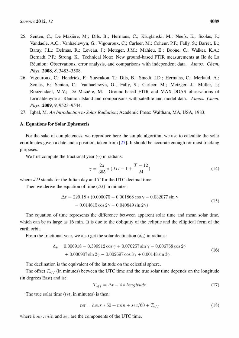
Figure A1. Comparison between the formulas reproduced in appendix and JPL ephemerides.

Figure A1 shows a comparison between the algorithm presented below and the Jet PropulsionLaboratory HORIZONS (http://ssd.jpl.nasa.gov/?horizons) ephemeris calculator. We compare thealtitude and azimuth of the Sun seen from Brussels (50.85◦N,4.35◦E) over a 30-year period, between1990 and 2020. Differences in altitude and azimuth are within 0.5◦.

c© 2012 by the authors; licensee MDPI, Basel, Switzerland. This article is an open access articledistributed under the terms and conditions of the Creative Commons Attribution license(http://creativecommons.org/licenses/by/3.0/).