EQUALITY OF OPPORTUNITY

By

John E. Roemer and Alain Trannoy

October 2013

COWLES FOUNDATION DISCUSSION PAPER NO. 1921

COWLES FOUNDATION FOR RESEARCH IN ECONOMICS YALE UNIVERSITY

Box 208281 New Haven, Connecticut 06520-8281

http://cowles.econ.yale.edu/

forthcoming, Handbook of Income Distribution September 17, 2013 A. Atkinson and F. Bourguignon (eds.)

“Equality of opportunity*”1

2by3

John E. Roemer 4and5

Alain Trannoy 67

1. Introduction 8

In the welfarist tradition of social-choice theory, egalitarianism means equality of 9

welfare or utility1. Conservative critics of egalitarianism rightly protest that it is highly 10

questionable that this kind of equality is ethically desirable, as it fails to hold persons 11

responsible for their choices, or for their preferences, or for the way they process 12

outcomes into some interpersonally comparable currency that one can speak of 13

equalizing. In political philosophy, beginning with John Rawls (1958, 1971), this 14

critique was taken seriously, and a new approach to egalitarianism transpired, which 15

inserted personal responsibility as an important qualifier of the degree of equality that is 16

ethically desirable. Thus, the development of egalitarian theory, since Rawls, may be 17

characterized as an effort to replace equality of outcomes with equality of opportunities, 18

where opportunities are interpreted in various ways. Metaphors associated with this 19

view are ‘leveling the playing field,’ and ‘starting gate equality.’ The main 20

philosophical contributions to the discussion were, following Rawls, from Amartya Sen 21

(1980), Ronald Dworkin (1981a, 1981b), Richard Arneson (1989) and G.A. Cohen 22

* We thank Tony Atkinson, François Bourguignon, Marc Fleurbaey, and Erik Schokkaert

for their comments on previous drafts of his chapter. 1 Welfarism is the view that social welfare (or the social objective function) should be

predicated only on the utility levels of individuals; that is, that the only information

required to compare social alternatives is that summarized in the utility-possibilities sets

those alternatives generate. It is a special case of consequentialism. See chapter 3 for

further discussion.

2

(1989)2. The debate is said to be about ‘equality of what,’ and the philosophical view is 23

sometimes called ‘luck egalitarianism,’ a term coined by Elizabeth Anderson (1999). 24

Economists (besides Sen) have been involved in this discussion from 1985 25

onwards. John Roemer (1993, 1998) proposed an algorithm for calculating policies that 26

would equalize opportunities for achievement of a given objective in a population. Marc 27

Fleurbaey and François Maniquet contributed economic proposals beginning in the 28

1990s, and recently summarized in Fleurbaey (2008). Other authors who have 29

contributed to the theory include Walter Bossert (1995, 1997), Vito Peragine (2004), and 30

Dirk Van de gaer ( 1993). An empirical literature is rapidly developing, calculating the 31

extent to which opportunities for the acquisition of various objectives are unequal in 32

various countries, and whether people hold views of justice consonant with equality of 33

opportunity.34

There are various ways of summarizing the significance of these developments 35

for the economics of inequality. Prior to the philosophical contributions that ignited the 36

economic literature that is our focus in this chapter, there was an earlier skirmish around 37

the practical import of equalizing opportunities. Just prior to the publication of Rawls’s 38

magnum opus (1971), contributions by Arthur Jensen (1969) and Richard Herrnstein 39

(1971) proposed that inequality was in the main due to differential intelligence (IQ), and 40

so generating a more equal income distribution by equalizing opportunities (for instance, 41

through compensatory education of under-privileged children) was a chimera.42

Economists Samuel Bowles (1973) and John Conlisk (1974) disagreed; Bowles argued 43

that inequality of income was almost all due to unequal opportunities, not to the 44

heritability of IQ. Despite this important debate on the degree to which economic 45

inequality is immutable, prior to Rawls, economists’ discussions of inequality were in the 46

main statistical, focusing on the best ways of measuring inequality.47

The post-Rawls-Dworkin inequality literature changed the focus by pointing out 48

that only some kinds of inequality are ethically objectionable, and to the extent that 49

2 The philosophical literature generated by these pioneers is to large to list here. Book-

length treatments that should be mentioned are Rakowski (1993) , Van Parijs (1997), and

Hurley (2003) .

3

economists ignore this distinction, they may be measuring something that is not ethically 50

salient. This distinction between morally acceptable and unacceptable inequality is 51

perhaps the most important contribution of philosophical egalitarian thought of the last 52

forty years. From the perspective of social-choice theory, equal-opportunity theory has 53

sharply challenged the welfarist assumption that is classically ubiquitous, maintaining 54

that more information than final outcomes in terms of welfare is needed to render social 55

judgment about the ranking of alternative policies – in particular, one must know the 56

extent to which individuals are responsible for the outcomes they enjoy -- whether those 57

outcomes were determined by social (and perhaps genetic) factors beyond their control, 58

or not – and this is non-welfare information.59

One must mention that another major non-welfarist theory of justice, but an 60

inegalitarian one, was proposed by Robert Nozick (1973) who argued that justice could 61

not be assessed by knowing only final outcomes; one had to know the process by which 62

these outcomes were produced. His neo-Lockean view, which proposed a theory of the 63

moral legitimacy of private property, can evaluate the justness of final outcomes only by 64

knowing whether the history that produced them was unpolluted by extortion, robbery, 65

slavery, and so on. Simply knowing the distribution of final outcomes (in terms of 66

income, welfare, or whatever) does not suffice to pass judgment on the distribution’s 67

moral pedigree. So the period since 1970 has been one in which, in political philosophy, 68

non-welfarist theories flourished, on both the right and left ends of the political spectrum.69

In this chapter, we begin by summarizing the philosophical debate concerning 70

equality since Rawls (section 2), presenting economic algorithms for computing policies 71

which equalize opportunities – or, more generally, ways of ordering social policies with 72

respect to their efficacy in opportunity equalization (sections 3, 4 and 5), application of 73

the approach to the conceptualization of economic development (section 6), discussion of74

dynamic issues (section 7), a preamble to a discussion of empirical work (section 8), 75

evidence of population views from surveys and experiments concerning conceptions of 76

equality (section 9), and a discussion of measurement issues, and summary of the 77

empirical literature on inequality of opportunity to date (section 10). We conclude with 78

mention of some critiques of the equal-opportunity approach, and some predictions 79

(section 11). 80

4

81

2. Egalitarian political philosophy since Rawls 82

John Rawls (1958) first published his ideas about equality over fifty years ago, 83

although his magnum opus did not appear until 1971. His goal was to unseat 84

utilitarianism as the ruling theory of distributive justice, and to replace it with a type of 85

egalitarianism. He argued that justice requires, after guaranteeing a system which 86

maximizes civil liberties, a set of institutions that maximize the level of ‘primary goods’ 87

allocated to those who are worst off in society, in the sense of receiving the least amount 88

of these goods. Economists call this principle ‘maximin primary goods;’ Rawls often 89

called it the difference principle. Moreover, he attempted to provide an argument for the 90

recommendation, based upon construction of a ‘veil of ignorance’ or ‘original position,’ 91

which shielded decision makers from knowledge of information about their situations 92

that was ‘morally arbitrary,’ so that the decision they came to regarding just allocation 93

would be impartial. Thus Rawls’s (1971) project was to derive principles of justice 94

from rationality and impartiality.95

Rawls did not advocate maxi-minning utility (even assuming interpersonal utility 96

comparisons were available), but rather maxi-minning (some index of) primary goods.97

This was, in part, his attempt to embed personal responsibility into the theory. For Rawls, 98

welfare was best measured as the extent to which a person is fulfilling his plan of life: but 99

he viewed the choice of life plan as something up to the individual, which social 100

institutions had no business passing judgment upon. Primary goods were deemed to be 101

those inputs that were required for the success of any life plan, and so equalizing 102

primary-goods bundles across persons (or passing to a maximin allocation which would103

dominate component-wise an equal allocation) was a way of holding persons responsible 104

for their life-plan choice. The question of how to aggregate the various primary goods 105

into an index that would allow comparison of bundles was never successfully solved by 106

Rawls (and some skeptical economists said that the subjective utility function was the 107

obvious way to aggregate primary goods).108

Rawls defended the difference principle by arguing that it would be chosen by 109

decision makers who were rational, but were deprived of knowledge about their own 110

situations in the world, to the extent that this knowledge included information about their 111

5

physical, social, and biological endowments, which were a matter of luck, and therefore 112

whose distribution Rawls described as morally arbitrary. He named the venue in which 113

these souls would cogitate about justice the ‘original position.’ In the original position, 114

souls were assumed to know the laws of economics, and to be self-interested. They were, 115

moreover, to be concerned with the allocation of primary goods, because they did not 116

know their life plans, or even the distribution of life plans in the actual society. Nor were 117

they to know the distribution of physical and biological endowments in society. 118

Here we believe Rawls made a major conceptual error. If the veil of ignorance 119

is intended to shield decision makers from knowledge of aspects of their situations that 120

are morally arbitrary, and only of those aspects, they should know their plans of life, 121

which, by hypothesis, are not morally arbitrary, because Rawls deems that persons are 122

responsible for their life plans. Secondly, although a person’s particular endowment of 123

resources, natural and physical, might well be morally arbitrary ( to the extent that these 124

were determined by the luck of the birth lottery), the distribution of these resources is a 125

fact of nature and society, and should be known by the denizens in the original position, 126

just as they are assumed to know the laws of economics. Therefore, Rawls constructed 127

his veil too thickly, on two counts, given his philosophical views.128

Given the paucity of information available to the decision makers in the original 129

position, it is not possible to use classical decision theory to solve the problem of the 130

desirable allocation of primary goods. Indeed, the only precise arguments that Rawls 131

gives for the conclusion that the difference principle would be chosen in the original 132

position occur at Rawls (1999[1971], p. 134), and they essentially state that decision 133

makers are extremely risk averse. For example: 134

135

The second feature that suggests the maximin rule is the 136following: the person choosing has a conception of the good such 137that he cares very little, if anything, for what he might gain about 138the minimum stipend that he can, in fact, be sure of by following 139the maximin rule. It is not worthwhile for him to take a chance 140for the sake of further advantage, especially when it may turn out 141that he loses much that is important to him. The last provision 142brings in the third feature, namely, that the rejected alternatives 143have outcomes one can hardly accept. The situation involves 144grave risks.145

6

146But extreme risk aversion, which Rawls here depends upon for his justification of 147

maximin, is certainly not an aspect of rationality.148

Thus, despite its enormous influence in political philosophy, Rawls’s argument 149

for maximin is marred in two ways: first, its reliance on deducing the principle of justice 150

from the original position was crucially flawed in depriving the denizens of that position 151

of knowledge of features of themselves (life plans) and of the world (the distributions of 152

various kinds of resources, including genetic ones, and ones possessed by families into 153

which a person is born) which were not morally arbitrary3, and second, for its assumption 154

(despite claims to the contrary by Rawls and others) that decision makers were extremely 155

risk averse. The value of Rawls’s contribution is in stating a radical egalitarian position 156

about the injustice of receiving resources through luck – and, in particular, the luck of the 157

birth lottery – and that it shifted the equalisandum from utility to a kind of resource, 158

primary goods. In our view, however, the project of deducing equality or maximin from 159

rationality and impartiality alone was a failure. Indeed, Moreno-Ternero and Roemer 160

(2008) argue that some solidaristic postulate is necessary to deduce maximin or, more 161

generally, to deduce some kind of egalitarianism as the ordering principle for social 162

choice. Although egalitarians might wish to deduce their view from postulates that can 163

garner universal approval (like rationality and impartiality), this is not possible.164

Therefore, an egalitarian theory of justice cannot have universal appeal, if the solidaristic165

postulate, which we believe necessary, is contentious. 166

Although Rawls is usually viewed as the most important egalitarian political 167

philosopher of the twentieth century, one may challenge the claim that his view is 168

egalitarian: to wit, the just income distribution, for Rawls, allows incentive payments to 169

the highly skilled in order to elicit their productive activity, even though this produces 170

inequality. The main philosopher who challenges Rawls’s acceptance of incentive-based 171

income inequality is G.A. Cohen, upon which more below.172

3 We reiterate it is the distribution of traits which is a fact of nature, and hence not

morally arbitrary, while the endowment of a given individual may well be morally

arbitrary, in the sense of being due to luck.

7

In 1981, Ronald Dworkin published two articles that essentially addressed the 173

problems in the Rawlsian argument that we have summarized, although he did not use the 174

Rawlsian language (original position, primary goods). His project was to define a 175

conception of equality that was ethically sound. In the first of these articles, he argued 176

that ‘equality of welfare’ was not a sound view, mainly because equality of welfare does 177

not hold persons responsible for their preferences. In particular, Dworkin argued that if 178

a person has expensive tastes, and he identifies with those tastes, society does not owe 179

him an additional complement of resources to satisfy them. (The only case of expensive 180

tastes, says Dworkin, that justifies additional resources are those tastes that are addictions 181

or compulsions, tastes with which the person does not ‘identify,’ and would prefer he did 182

not have.) In the second article, Dworkin argues for ‘equality of resources,’ where 183

resources include (as for Rawls) aspects of a person’s physical and biological 184

environment for which he should not be held responsible (such as those acquired through 185

birth).186

But how can one ‘equalize resources,’ when these comprise both transferable 187

goods, like money, and inalienable resources, like talents, families into which persons are 188

born, and even genes? Dworkin proposed an ingenious device, an insurance market 189

carried out behind a veil of ignorance, where the ‘souls’ participating represent actual 190

persons, and know the preferences of those whom they represent, but do not know the 191

resources with which their persons are actually endowed in the world. In this insurance 192

market, each participant would hold an equal amount of some currency, and would be 193

able to purchase insurance with that currency against bad luck in the birth lottery, that is, 194

the lottery in which nature assigns souls to persons in the world (or resource endowments 195

to souls). Dworkin argued that the allocation of goods that would be implemented after 196

the birth lottery occurred, the state of the world was revealed, and insurance policies 197

taken behind the Dworkinian veil were settled, was an allocation that ‘equalized 198

resources.’ It held persons responsible for their preferences – in particular, their risk 199

preferences—and was egalitarian because all souls were endowed, behind the veil, with 200

the same allotment of currency with which to purchase insurance. Impartiality with 201

respect to the morally arbitrary distribution of resources was accomplished by shielding 202

the souls from knowledge of their endowments in the actual world associated with the 203

8

birth lottery (genetic and physical). Thus, Dworkin retained Rawls’s radical egalitarian 204

view about the moral arbitrariness of the distribution of talents, handicaps, and inherited 205

wealth, but implemented a mechanism that held persons responsible for their tastes that 206

was much cleaner than discarding preferences and relying on primary goods, as Rawls 207

had done. 208

Despite the cleverness of Dworkin’s construction, it can lead to results that many 209

egalitarians would consider perverse. To illustrate the problem, consider the following 210

example. Suppose there are two individuals in the world, Andrea and Bob. Andrea is 211

lucky: she has a fine constitution, and can transform resources (wealth) into welfare at a 212

high rate. Bob is handicapped; his constitution transforms wealth into welfare at exactly 213

one-half of Andrea’s rate. We assume, in particular, that Andrea and Bob have 214

interpersonally comparable welfare. The internal resource that Andrea possesses and 215

Bob lacks is a fine biological constitution (say, a healthy supply of endorphins).216

We assume that Bob and Andrea have the same risk preferences over wealth: they 217

are each risk averse and have the von Neumann – Morgenstern utility function over 218

wealth . Suppose that the distribution of (material) wealth in the world to 219

(Andrea, Bob) would be , with no further intervention. Thus each individual is 220

endowed with an internal constitution and some external resource. 221

We construct Dworkin’s hypothetical insurance market as follows4. Behind the 222

veil of ignorance, there is a soul Alpha who represents Andrea, and a soul Beta who 223

represents Bob. These souls know the risk preferences of their principals, and the 224

constitutions of Andrea and Bob, but they do not know which person they will become in 225

the birth lottery. Thus, from their viewpoint, there are two possible states of the world, 226

summarized in the table: 227

228

229

State 1 Alpha becomes Andrea Beta becomes Bob

State 2 Alpha becomes Bob Beta becomes Andrea

4 Dworkin did not propose a formal model, but relied on intuition. The model here is a

version of an Arrovian market for contingent claims.

u(W ) = W

(W A ,W B )

9

230

Each state occurs with probability one-half. We know that state 1 will indeed occur, but 231

the souls face a birth lottery with even chances, in which they can take out insurance 232

against bad luck (that is, of becoming Bob). 233

There are two commodities in the insurance market: a commodity , a unit of 234

which pays the owner $1 if state 1 occurs, and a commodity a unit of which pays $1 if 235

state 2 occurs. Each soul can either purchase or sell these commodities: selling one unit 236

of the first commodity entails a promise to deliver $1 if state 1 occurs. Each soul 237

possesses, initially, zero income (behind the veil) with which to purchase these 238

commodities. In particular, they have equal wealth endowments behind the veil in the 239

currency that is recognized in that venue. Thus, the insurance market acts to redistribute 240

tangible wealth in the actual world to compensate persons for their natural endowments, 241

which cannot be altered, in that way which the souls, who represent persons, would 242

desire, had they been able to insure against the luck of the birth lottery. It is an institution 243

that transforms what Dworkin calls ‘brute luck’ into ‘option luck.’ The former is luck 244

which is not insurable; the latter is luck whose outcome is protected by insurance, or the 245

outcome of a gamble one has chosen to take. 246

An equilibrium in this insurance market consists of prices for commodities 247

, demands by souls Alpha and Beta for the two contingent 248

commodities, such that249

(1) 250

(2)251

(3) . 252

Let us explain these conditions. Condition (1) says that Alpha chooses her 253

demand for contingent commodities optimally, subject to her budget constraint – that is, 254

x1

x2

(1, p)

(x1,x2 ) (x1 ,x2 ),(x1 ,x2 )

(x1 ,x2 ) maximizes 12

W A + x1 + 12

W B + x2

2subj. to x1 + px2 = 0

(x1 ,x2 ) maximizes 12

W B + x1 + 12

2(W A + x2 )

subj. to x1 + px2 = 0

xs + xs = 0 for s = 1,2

10

she maximizes her expected utility. Her utility if she becomes Andrea (state 1), will be 255

. Now if Alpha becomes Bob (state 2), her wealth will be ; 256

however, from the viewpoint of her principal, Andrea, that will generate only half as 257

much welfare, so she evaluates this wealth as being worth, in utility terms, . 258

Condition (2) has a similar derivation, but this time, soul Beta takes the benchmark 259

situation as becoming Bob. Condition (3) says that both markets clear. 260

The equilibrium is given by 261

262

Now state 1 occurs. Therefore Andrea, after the insurance contracts are settled, ends up 263

with wealth -- two-thirds of the total wealth—and Bob ends up 264

with one-third of the total wealth. The result is perverse because, Bob is the one with the 265

low resource endowment, that is, with a low ability to transform money into welfare. It 266

is Bob, putatively, whom an equal-resource principle should compensate, but it is Andrea 267

who ends up the winner.5 Even should state 2 have occurred, the outcome would have 268

been the same – two-thirds of the wealth would end up being Andrea’s.269

5 This perversity of the Dworkin insurance mechanism was first pointed out by Roemer

(1985). Dworkin never proposed a model of the insurance market, but conjectured that it

would re-allocate wealth in a way to compensate those with a paucity of non-transferable

resources. He continued to use the insurance-market thought experiment to justify social

policies (e.g., in the case of national health insurance for the United States), even though

his thought experiment did not necessarily produce the compensatory redistributions that

he thought it would implement.

W1A + x1 W B + x2

W B + x2

2

p = 1, (x1 ,x2 ) = (2W B W A

3,W

A 2W B

3), (x1 ,x2 ) = ( 2W B +W A

3, W A + 2W B

3).

W A + x1 = 23

(W A +W B )

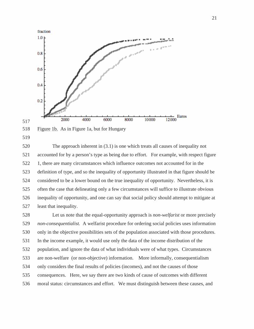
11

Why does this happen? Because, even though both souls are risk averse, they are 270

not sufficiently risk averse to induce them to shift wealth into the bad state (of being born 271

Bob); it is more worthwhile (in terms of expected utility) to use wealth in the state when 272

it can produce a lot of welfare (when a soul turns out to be Andrea). If the agents were 273

sufficiently risk averse, this would not occur. (If the utility function were , 274

and , then, post-insurance, Bob would end up with more wealth than Andrea. If the 275

utility function is u(W ) = logW , then the agents split the wealth equally.) But the 276

example shows that in general the hypothetical insurance market does not implement the 277

kind of compensation that Dworkin desires: for Bob is the one who suffers from a deficit 278

in an internal resource – from morally arbitrary bad luck. For Dworkin’s insurance 279

market to avoid this kind of perversity, individuals would have to be sufficiently risk 280

averse, and this it is inappropriate to assume, for the theory should surely produce the 281

desired result (of compensating those with a paucity of internal resources) in the special 282

case that all agents have the same risk preferences6.283

In the model just presented of the hypothetical insurance market, note that it was 284

necessary to make interpersonal welfare comparisons. Alpha, Andrea’s soul, has to 285

contemplate how she would feel, if she were to be born as Bob, and with a given amount 286

of wealth. She does this by transforming Bob’s wealth into a welfare-equivalent wealth287

for Andrea. And soul Beta has to make a similar interpersonal comparison. We 288

maintain that it is impossible to construct a veil-of-ignorance thought experiment without 289

making such comparisons. The point is simple: if a soul has to compare how it would 290

feel when being incarnated as different persons, it must be able to make interpersonal 291

6 When Dworkin was confronted with this example at a conference in Halifax in 1985, he

responded that he would not use the insurance device in cases where it produced the

‘pathological’ result. This is, however, probably an unworkable position, for how does

one characterize a priori the set of admissible economic environments?

This is not the first time that insufficient concavity of preferences causes problems

for economic analysis. See, for example, the discussion of money-metric utility in

chapter 3.

u(W ) =W c / c

c < 0

12

welfare comparisons. Without the ability to compare the lives of different persons in 292

different circumstances, an investment in insurance would have no basis7.293

Despite the problem we have exhibited with Dworkin’s proposal, it was 294

revolutionary, in the words of G.A. Cohen, in transporting into egalitarian theory the 295

most powerful tool of the anti-egalitarian Right, the importance of personal responsibility. 296

One might argue, after seeing the above demonstration, that Dworkin’s insurance market 297

is an appealing thought experiment, and therefore one should give up on the egalitarian 298

impulse of compensating persons for features of their situations for which they are not 299

responsible: that is, instead of rejecting Dworkin’s model as inadequate, one should reject 300

his egalitarian desideratum. Moreno and Roemer (2008) consider this, and argue instead 301

that the veil of ignorance is an inappropriate thought experiment for ascertaining what 302

justice requires. Although their arguments for this are new, the position is not: it was also 303

advocated earlier by Brian Barry (1991).304

In the example we have given, there is, for egalitarians, a moral requirement to 305

transfer tangible wealth from Andrea to Bob, because Bob lacks an inalienable resource 306

that Andrea possesses, the ability to transform effectively goods into welfare, a lack 307

which is beyond his control, and due entirely to luck. Dworkin also focused upon a 308

different possible cause of unequal welfares, that some persons have expensive tastes, 309

while others have cheap ones. His view was that persons with expensive tastes do not310

merit additional wealth in order to satisfy them, as long as those persons were satisfied 311

with their tastes, or, as he said, identified with them. There is no injustice in a world 312

where wealth is equal, but those with champagne tastes suffer compared to those with 313

beer tastes, due to the relative consumptions of champagne and beer that that equal 314

wealth permits. So the ‘pathology’ that we have illustrate with the Andrea-Bob example 315

7 Readers may recall that Harsanyi (1955) claimed to construct a veil-of-ignorance

argument for utilitarianism without making interpersonal comparisons. But his argument

fails – not as a formal mathematical statement, but in the claim that utilitarianism is what

has been justified. (See, for an early discussion, Weymark (1991), and for a more recent

one, Moreno-Ternero and Roemer (2008).)

13

depends upon the source of Bob’s relative inefficiency in converting wealth into welfare 316

being a handicap, rather than an expensive taste. 317

Slightly before Dworkin’s articles were published, Amartya Sen (1980) gave a 318

lecture in which he argued that Rawls’s focus on primary goods was misplaced. Sen 319

argued that Rawls was ‘fetishist’ in focusing on goods, and should instead have focused 320

on what goods provide for people, which he called ‘functionings’ – being able to move 321

about, to become employed, to be healthy, and so on. Sen defined a person’s capability322

as the set of vectors of functionings that were available to him, and he called for equality 323

of capabilities8. Thus, although a rich man on a hunger strike might have the same (low) 324

functioning as a poor man starving, their capabilities are very different. While not going 325

so far as to say utilities should be equalized, Sen defined a new concept between goods 326

and welfare – functionings—which G.A. Cohen (1993) later described as providing a 327

state of being that he called ‘midfare.’ For Sen, the opportunity component of the theory 328

was expressed in an evaluation not of a person’s actual functioning level, but of what 329

functionings were available to him, his ‘capability.’330

Sen’s contribution led to both theoretical and practical developments. On the 331

theoretical level, it inspired a literature on comparing opportunity (or feasible) sets: if one 332

desires to ‘equalize’ capabilities, it helps to have an ordering on sets of sets. See James 333

Foster’s (2011) summary of this literature. On the practical side, it led to the human 334

development index, published annually by the UNDP. For development of Sen’s 335

capability approach, see chapter 3.336

Later in the decade, further reactions to Dworkin came from philosophers, notably 337

Richard Arneson (1989) and G.A. Cohen (1989). Arneson argued that Dworkin’s338

expensive-taste argument against equality-of-welfare was correct, but his alternative of 339

seeking equality of resources was not the only option: instead, one should seek to 340

equalize opportunities for welfare. This, he argued, would take care of the expensive-341

tastes problem. Rather than relying on the insurance mechanism to define what resource 342

egalitarianism means, Arneson proposed to distribute resources so that all persons had 343

equal opportunity for welfare achievement, although actual welfares achieved would 344

8 Sen has not proposed an ordering of sets that would enable one to compare capabilities.

14

differ because people would make different choices. There are problems with 345

formalizing Arneson’s proposal (see Roemer (1996)) , but it is notable for not relying on 346

any kind of veil of ignorance, in contrast to the proposals of Rawls and Dworkin. 347

Cohen (1989) criticized Dworkin for making the wrong ‘cut’ between resources 348

and preferences. The issue, he said, was what people should or should not be held 349

responsible for. Clearly, a person should not be held responsible for his innate talents 350

and inherited resources, but it is not true that a person should be fully responsible for his 351

preferences either, because preferences are to some (perhaps large) degree formed in 352

circumstances (in particular, those of one’s childhood) which are massively influenced by 353

resource availability. Indeed, if a person has an expensive taste for champagne due to a 354

genetic abnormality, he would merit compensation under an egalitarian ethic9. Cohen’s 355

view was that inequality is justified if and only if it is attributable to choices that are ones 356

for which persons can sensibly he held responsible -- so if a person who grows up poor, 357

develops a ‘taste’ against education, induced by the difficulty of succeeding in school due 358

to lack of adequate resources – a taste with which he even comes to ‘identify’ – then 359

Cohen would not hold him responsible for the low income due to his consequently low 360

wage, while Dworkin presumably would hold him responsible. Cohen does not propose 361

a mechanism or algorithm for finding the just distribution of resources, but provides a 362

number of revealing examples (see, for example, Cohen (1989, 2004)). He calls his 363

approach ‘equal access to advantage.’364

Besides criticizing Dworkin for his partition the space of attributes and actions 365

into ones for which compensation is, or is not, due, Cohen (1997), importantly, critiqued 366

Rawls’s difference principle, as insufficiently egalitarian. The argument is based upon 367

Rawls’s restriction of the ambit of justice to the design of social institutions – in 368

particular, that ambit does not include personal behavior. Thus, the Rawlsian tax system 369

should attempt to maximize the welfare of the least-well-off group in society, under the 370

assumption that individuals choose their labor supplies to maximize their personal utility.371

9 This is not a crazy example. There is a medically recognized syndrome in which people

who sustain a certain kind of brain injury come to crave expensive foods: see Cohen

(2011, p. 81).

15

Suppose the highly skilled claim that if their taxes are raised from 30% to 50%, they will 372

reduce their labor supply so much that the worst-off group would be less well off than it 373

is at the 30% tax rate. If 30% is the tax rate that maximizes the welfare (or income) of 374

the least well off, given this self-interested behavior of the highly skilled, then it is the 375

Rawlsian-just rate. But Cohen responds that, as long as the highly skilled are at least as 376

well off as the worst off at the 50% tax rate, then justice requires the 50% tax rate. This 377

difference of viewpoint between Rawls and Cohen occurs because Cohen requires 378

individuals to act, in their personal choices, according to the commands of the difference 379

principle (that is, to take those actions that render those who are worst off as well off as 380

possible), and Rawls does not. Indeed, Rawls stipulates that one requirement of a just 381

society is that its members endorse the conception of justice. It is peculiar, Cohen 382

remarks, that that conception should apply only to the design of social institutions, and 383

not to personal behavior.384

A question that arises from the discussion of responsibility is its relationship to 385

freedom of the will. If responsibility has become central in the conceptualization of just 386

equality, does one have to solve the problem of free will before enunciating a theory of 387

distributive justice? Different answers are on offer. We believe the most practical 388

answer, which should suffice for practicing economists, is to view the degree of 389

responsibility of persons as a parameter in a theory of equality. Once one assigns a value 390

to this parameter, then one has a particular theory of equality of opportunity, because one 391

then knows for what to hold persons responsible. The missing parameter is supplied by 392

each society, which has a concept of what its citizens should be held responsible for; 393

hence there is a specific theory of equality of opportunity for each society, that is, a 394

theory that will deliver policy recommendations consonant with the theory of 395

responsibility that that society endorses. This is a political approach, rather than a 396

metaphysical one. 397

Another answer to the free-will challenge is to make a distinction prevalent 398

among philosophers. ‘Compatibilists’ are those philosophers who believe that it is 399

consistent both to endorse determinism (in the sense of a belief in the physical causation 400

of all behavior) and the possibility of responsibility; incompatibilists are those who 401

believe that determinism precludes responsibility. Most philosophers (who think about 402

16

the problem) are probably, at present, compatibilists. For instance, Thomas Scanlon 403

(1986) believes that the determinist causal view is true, but also that persons can be held 404

responsible for their behavior, as long as they have contemplated their actions, weighed 405

alternatives, and so on. (The issue of sufficient contemplation is independent of the 406

issue of the cause of expensive tastes, raised above.) From a practical viewpoint, the 407

problem of free will therefore does not pose a problem for designing policies motivated 408

by the idea that persons should not be held accountable for aspects of their condition that 409

are due to circumstances beyond their control. 410

The philosophical literature on ‘responsibility-sensitive egalitarianism’ continues 411

beyond the point of this quick review, but enough summary has been provided to proceed 412

to a discussion of economic models. 413

414

3. A model and algorithm for equal-opportunity policy 415

Consider a population, whose members are partitioned into a finite set of types. A 416

type comprises the set of individuals with the same circumstances, where circumstances417

are those aspects of one’s environment (including, perhaps, one’s biological 418

characteristics) which are beyond one’s control, and influence outcomes of interest.419

Denote the types . Let the population fraction of type t in the population be 420

. There is an objective for which a planner wishes to equalize opportunities. The 421

degree to which an individual will achieve the objective is a function of his circumstances, 422

his effort, and the social policy: we write the value of the objective as , where e423

is a measure of effort and , the set of social policies. Indeed, should be 424

considered the average achievement of the objective among those of type t expending 425

effort e when the policy is . Here, we will take effort to be a non-negative real number. 426

Later, we will introduce luck into the problem. 427

is not, in general, a subjective utility function: indeed is assumed to be 428

monotone increasing in effort, while subjective utility is commonly assumed to be 429

decreasing in standard conceptions of effort. Thus, u might be the adult wage, 430

circumstances could include several aspects of childhood and family environment, and e431

could be years of schooling. Effort is assumed to be a choice variable for the individual, 432

t = 1,...,T

f t

ut (e, )

ut (e, )

ut ut

17

although that choice may be severely constrained by circumstances, a point to which we 433

will attend below. The final data for the problem consist of the distributions of effort 434

within types as a function of policy: for the policy , denote the distribution function of 435

effort in type t as Gt ( ) . We would normally say that effort is chosen by the individual 436

by maximizing a preference order, but preferences are not the fundamentals of this 437

theory: rather, the data are {T ,Gt , f t ,u, } , where we use T to denote, also, the set of 438

types.439

Defining the set of types and the conception of effort assumes that the society in 440

question has a conception of the partition between responsible actions and circumstances, 441

with respect to which it wishes to compute a consonant approach to equalizing 442

opportunities. We describe the approach of Roemer (1993, 1998). The verbal statement 443

of the goal is to find that policy which nullifies, to the greatest extent possible, the effect 444

of circumstances on outcomes, but allows outcomes to be sensitive to effort. Effort 445

comprises those choices that are thought to be the person’s responsibility, and hence they 446

are consequences of his choices – but not all such consequences, since effort may itself 447

be influenced by one’s circumstances. In particular, the distribution of effort in a type at 448

a policy, , is not due to the actions of any person (assume here a continuum of agents), 449

but is a characteristic of the type. If we are to indemnify individuals against their 450

circumstances, we must not hold them responsible for being members of a type with a 451

poor distribution of effort.452

We require a measure of accountable effort, which, because effort is influenced 453

by circumstances, cannot be the raw effort e. (Think of years of education – raw effort—454

which is surely influenced in a major way by social circumstances.) Roemer proposed to 455

measure accountable effort as the rank of an individual on the effort distribution of her 456

type: thus, if for an individual expending effort e, , we say the individual 457

expended the degree of effort , as opposed to the level of effort e. The rank provides a 458

way of making inter-type comparisons of the efforts expended by individuals. A person 459

is judged accountable, that is to say, by comparing his behavior only to others with his 460

circumstances. In comparing the degrees of effort of individuals across types, we use the 461

Gt

Gt (e) =

18

rank measure, which sterilizes the distribution of raw effort of the influence of 462

circumstances upon it10.463

Because the functions are assumed to be strictly monotone increasing in e, it 464

follows that an individual will have the same rank on the distribution of the objective, 465

within his type, as he does within the distribution of effort of his type11. Define: 466

467

where is the level of effort at the quantile of the distribution , that is, 468

. Then the functions are the inverse functions of the distribution 469

functions of the objective, by type, under the policy . (In this sense, vt is like Pen’s 470

parade, which is also the inverse of a distribution function.) Inequality of opportunity 471

holds when these functions are not identical. In particular, because we are viewing 472

persons at a given rank as being equally accountable with respect to the choice of 473

effort, the vertical difference between the functions is a measure of the extent 474

of inequality of opportunity (or, equivalently, the horizontal distance between the 475

cumulative distribution functions). 476

What policy is the optimal one, given this conception? We do not simply want to 477

render the functions identical at a low level, so we need to adopt some conception of 478

‘maxi-minning’ these functions. We want to choose that policy which pushes up the 479

lowest vt function as much as possible – and as in Rawlsian maximin, the ‘lowest’ 480

function may itself be a function of what the policy is. A natural approach is therefore to 481

10 Some authors (Ramos and Van de gaer (2012)) have called this move – of identifying

the degree of effort with the rank of the individual on the objective distribution of his

type – the Roemer Identification Assumption (RIA). While the name is lofty, the idea is

simple: persons should not be held responsible for characteristics of the distribution of

effort in their type, for that distribution is a circumstance. 11 If actual effort is a vector, then a unidimensional measure e would be constructed, for

example, by regressing the objective values against the dimensions, thus computing

weights on the dimensions of raw effort.

ut

vt ( , ) = ut (et ( ), )

et ( ) th Gt

Gt (et ( )) := vt ( , )

{vt ( , )}

vt

19

maximize the area below the lowest function , or more precisely, to find that policy 482

which maximizes the area under the lower envelope of the functions . The formal 483

statement is to: 484

. (3.1) 485

We call the solution to this program the opportunity-equalizing policy, . 486

(Computing (3.1) is equivalent to maximizing the area to the left of the left-hand 487

envelope of the type-distributions of the objective, and bounded above by the horizontal 488

line of height one.) 489

In the case in which the lower envelope of the functions is the function of a 490

single type (the unambiguously most disadvantaged type), what we have done is simply 491

to maximize the average value of the objective for the most disadvantaged type, since 492

is simply the mean value of the objective for type t at policy . 493

Thus, the approach implements the view that differences between individuals 494

caused by their circumstances are ethically unacceptable, but differences due to 495

differential effort are all right. Full equality of opportunity is achieved not when the 496

value of the objective is equal for all, but when members of each type face the same497

chances, as measured by the distribution functions of the objective that they face. 498

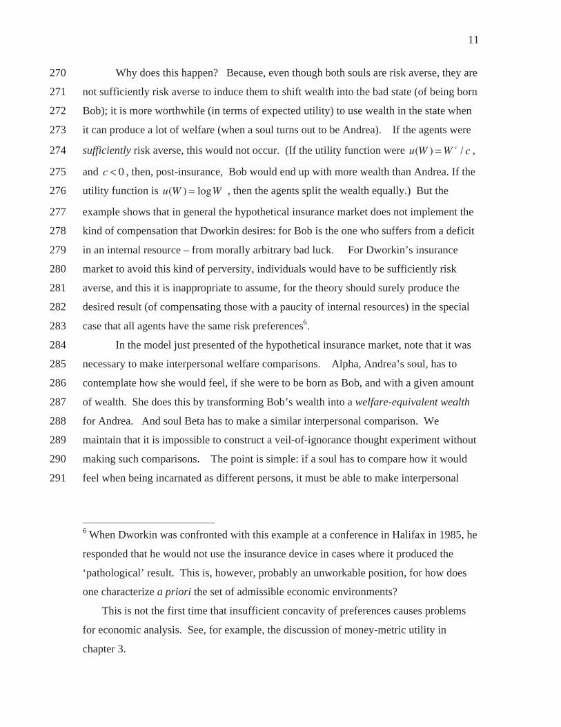
One virtue of the approach taken here is that it is easy to illustrate graphically. In 499

Figure 1, we present two graphs, to illustrate inequality of opportunity in Hungary and 500

Denmark. In each graph, there are three cumulative income distributions, corresponding 501

to male workers of three types: those whose more educated parent had no more than 502

lower secondary education, those whose more educated parent just completed secondary 503

education, and those whose more educated parent had at least some tertiary education.504

(The data are from EU-SILC-2005.) The inverses of these distribution functions are the 505

functions defined above. The policy is the status-quo policy. It seems clear that, 506

with respect to this one circumstance (parental education), opportunities for income have 507

vt

{vt}

max mint

vt ( , )d0

1

EOp

{vt}

vt ( , )d0

1

vt ( , )

20

been more effectively equalized in Denmark than in Hungary12. The graphs are taken 508

from Roemer (2013).509

510

511512

Figure 1a Three income distribution functions for Danish male workers, according the 513

circumstance of parental education. (Darkest hue are from least highly educated 514

backgrounds)515

516

12 We say ‘seems’ clear, because the horizontal-axis Euro scale is different in the two

figures.

21

517Figure 1b. As in Figure 1a, but for Hungary 518

519

The approach inherent in (3.1) is one which treats all causes of inequality not 520

accounted for by a person’s type as being due to effort. For example, with respect figure 521

1, there are many circumstances which influence outcomes not accounted for in the 522

definition of type, and so the inequality of opportunity illustrated in that figure should be 523

considered to be a lower bound on the true inequality of opportunity. Nevertheless, it is 524

often the case that delineating only a few circumstances will suffice to illustrate obvious 525

inequality of opportunity, and one can say that social policy should attempt to mitigate at 526

least that inequality.527

Let us note that the equal-opportunity approach is non-welfarist or more precisely 528

non-consequentialist. A welfarist procedure for ordering social policies uses information 529

only in the objective possibilities sets of the population associated with those procedures.530

In the income example, it would use only the data of the income distribution of the 531

population, and ignore the data of what individuals were of what types. Circumstances 532

are non-welfare (or non-objective) information. More informally, consequentialism533

only considers the final results of policies (incomes), and not the causes of those 534

consequences. Here, we say there are two kinds of cause of outcomes with different 535

moral status: circumstances and effort. We must distinguish between these causes, and 536

22

social policy should attempt to mitigate the inequality effects of one of them, but not 537

necessarily of the other. 538

At this point, we return briefly to consider a philosophical critique of this 539

approach – and indeed of the general evolution of responsibility-sensitive egalitarianism, 540

as it was reviewed in section 1 above – offered by Susan Hurley (2002), who writes that 541

“Roemer’s account does not show how the aim to neutralize luck could provide a basis 542

for egalitarianism.” Hurley says that, absent luck, many possible distributions of the 543

objective could have occurred, and one cannot claim that ‘neutralizing’ luck means to 544

render outcomes sensitive only to degrees of effort. Moreover, she writes that it is not 545

an argument for EOp that it neutralizes the effects of luck. 546

The moral premise of the EOp view is that rewards should be sensitive only to the 547

autonomous efforts of individuals. This is a special case of rewards according to deserts. 548

People deserve, in the EOp view, to acquire the objective in proportion to how hard they 549

try. Thus, strictly speaking, the EOp view is not one whose fundamental primitive is 550

equality: deservingness is fundamental, together with the normative thesis that justified 551

inequality tracks deservingness. Inequalities that are not due to unequal efforts are 552

defined as being due to luck: that is, luck is so-called because it is a cause of reward that 553

is illegitimate from the EOp view. The statement that ‘EOp intends to neutralize the 554

effects of luck on outcomes’ is therefore equivalent to the statement ‘EOp intends to 555

render outcomes sensitive only to effort.’ 556

So, for example, suppose a child, A, does well in life because his parents were 557

rich, not because he exerted great effort, while another child, B, from a poor family, does 558

well by virtue of exerting great effort. Some might argue that it may be no less a matter 559

of luck that B was the kind of person who works hard than that A had rich parents, but 560

that approach, whatever its merits, is not the sense in which responsibility-concerned 561

egalitarians use the word luck. Luck, for us, means the source of non-effort caused 562

advantage. To be sure, it is not an argument for EOp that it neutralizes luck, it is rather 563

definitive of the EOp view that it does so. The argument for EOp must be that is right to 564

render outcomes sensitive only to effort13. 565

13 This point is due to Cohen (2006).

23

The next example, which is hypothetical, is given to illustrate the difference 566

between the equal-opportunity approach and the approach that is conventional in many 567

areas of social policy, utilitarianism. A utilitarian policy maximizes the average value 568

of the objective in a population. Utilitarianism is a special case of welfarism, although 569

there are many welfarist preference orderings of policies.570

We consider a population partitioned into T types, where the frequency of type t is 571

. The population suffers from I diseases, with the generic disease denoted i. The 572

types might be defined by socio-economic characteristics14, and the Health Ministry is 573

interested in mitigating the affect of socio-economic characteristics on health. There is 574

available in the health sector an amount of resource (money), per capita. We do not 575

address how much of a society’s product should be dedicated to health, but only how to 576

spend the amount that has been so dedicated. Effort is here conceived of as life-style 577

quality (exercise, smoking behavior, etc.). We choose the policy space to be allocations 578

of the resource to treating various diseases: that is vectors which will be 579

constrained by a budget condition, where Ri is the amount that will be spent to treat 580

each case of disease i, regardless of the characteristics of the person who has contracted 581

the disease. Thus, by definition, we restrict ourselves to policies that are horizontally582

equitable: any person suffering from disease i, regardless of her type and life-style quality, 583

will receive the same treatment, because treatment expenditure is not a function of these 584

variables. A more highly articulated policy space could allocate medical resources 585

predicated also on the type of patient and the life-style that patient had led. But in the 586

health sector, doing so would set the stage for antagonistic patient-provider relations, and 587

interfere with other values we hold, and so we choose to respect horizontal equity. We 588

will return to this point below.589

For any given vector R = (x1,..., xI ) there will ensue a distribution of life-style 590

quality in each type t, and a consequent distribution of disease occurrences in each type. 591 14 Of course, persons are surely in part responsible for their socio-economic

circumstances. But the Health Ministry’s mandate might be to eliminate health

inequalities due those circumstances, and so formally, it would consider socio-economic

aspects of households as circumstances.

f t

R

R = (R1,..., RI )

24

Life-style quality may not be responsive to the policy, but we allow for the general case 592

in which it is. Let us denote the fraction of individuals in type t who contract disease i593

when the policy is R by . Then the policy is feasible when: 594

f t pit (R)xi Ri,t

595

and it exhausts the budget precisely when: 596

f t pit (R)xi = Ri,t

(3.2) 597

The set of admissible policies comprises all those for which (3.2) holds: this is the set . 598

We next suppose that we know the health production functions for each type; 599

these are functions that give the probability that a person of type t will contract disease i600

if she lives a life-style of quality q. Let i = 0 represent the case of ‘no disease’ being 601

contracted. We denote these functions ; thus is the probability that a t- type 602

will contract disease i if she lives life-style quality q. We presume it is the case that 603

{ } are monotone decreasing functions: that is, raising life-style quality reduces the 604

probability of disease. 605

We also have as data of the problem the mapping from the policy space to the 606

space of cumulative distribution functions on the non-negative real numbers. Denote that 607

class of distribution functions by . The map 608

609

gives us the distribution of life-style qualities that will occur in type t, at any policy R in 610

. We write . Thus an individual with life-style quality q in type t lies at 611

rank of the effort distribution of her type, when the policy is R, if We 612

denote this value of q by qRt ( ) . 613

Finally, we need to postulate the relationship between treatment of disease and 614

health outcome. Let us take the outcome to be life expectancy. We therefore suppose 615

that we know the life expectancy for those in type t who have contracted disease i and 616

who are treated with the resource expenditure specified by R. Denote this life expectancy 617

by it (R) . (Denote by 0t the life expectancy of a person of type t who contracts no 618

pit (R)

sit ( ) sit (q)

sit

F t :

FRt = F t (R)

FRt (q) = .

25

disease.) We could further complexify, here, by assuming that life expectancy is a 619

function, in addition, of the life style quality of the individual, but choose not to do so. 620

Consider, now, a policy R = (x1,..., xI ) , which induces a distribution of life-style 621

quality in each type. Consider a type t and all those at rank of t’s life-style quality 622

distribution. Assume there is a large number of people in each type, so that the fraction 623

of people in a type who contract a disease is equal to the probability that people in that 624

type will contract the disease. Then15 the average life expectancy of all such people – the 625

(t, ) cohort—will be626

s0t (qRt ( )) 0t + sit (qR

t ( )ti=1

I

) it (R) Lt ( ,R) .627

We can now define the EOp policy, which is: 628

REOp = argmaxR

mint0

1

Lt ( ,R)d (3.3) 629

Although we need a lot of data to compute the EOp policy, it is only the Ministry 630

of Health who must have these data: once the policy is computed, a hospital need only631

diagnose a patient to know what treatment is appropriate (i.e., how much to spend on the 632

case). No patient need ever be asked her type or her life-style characteristics. There is, 633

that is to say, no incursion of privacy necessitated by applying the policy—apart from the 634

initial incursion in the research survey on a population sample that assembles the data set 635

to compute the health production functions. The policy is horizontally equitable. This is 636

an important point, because some philosophers have falsely concluded that applying the 637

equal-opportunity approach will necessitate incursions into privacy, and making 638

distinctions among individuals in resource-allocation questions that are either difficult or 639

socially objectionable in some way (see Anderson (1999)). But this is incorrect: the 640

planner can choose the policy space in a way that makes such distinctions irrelevant for 641

implementing the policy. In other words, not only is the delineation of circumstances a 642

15 In the formula that follows, we have assumed for the sake of simplicity that an

individual contracts either no or one disease. Of course, the formula can be generalized

to the case where we drop this assumption, as we do in the numerical example that

follows.

26

political/social decision that may vary across societies, but so must the specification of 643

the policy space take into consideration social views concerning privacy and fairness. 644

Let us make this example numerical. We posit a society with two types, the Rich 645

and the Poor. The Poor have life-styles whose qualities q are uniformly distributed on 646

the interval [0,1], while the Rich have life-style qualities that are uniformly distributed on 647

the interval [0.5, 1.5]. The probability of contracting cancer, as a function of life-style 648

quality (q) is the same for both types, and given by: 649

650

Only the poor are at a risk of tuberculosis; their probability of contracting TB is: 651

652

Suppose that life expectancy for a rich individual is given by: 653

70, if cancer is not contracted, and 654

, if cancer is contracted, and xc is spent on its treatment. 655

Thus, if the disease is contracted, life expectancy will lie between 50 and 70, depending 656

on how much is spent on treatment (from zero to an infinite amount). This is a simple 657

way of modeling the fact that nobody dies of cancer before age 50. 658

Suppose that life expectancy for a Poor individual is: 659

70 if neither disease is contracted, 660

if cancer is contracted and xc is spent on its treatment, and661

if tuberculosis is contracted and is spent on its treatment. 662

Thus, the Poor can die at age 30 if they contract TB and it is not treated. With large 663

expenditures, a person who contracts TB can live to age 70. Furthermore, it is expensive 664

to raise life expectancy above 30 if TB is contracted. We further assume that if a Poor 665

person contracts both cancer and TB then her life expectancy will be the minimum of the 666

above two numbers. 667

Finally, assume that 25% of the population is poor and 75% is rich, and that the 668

national health budget is R = $3000 per capita. 669

sCP (q) = sCR (q) = 12q3.

sTP (q) = 1q3.

60 +10xc 1

xc +1

60 +10xc 1

xc +1

50+ 20.1xTB 1.1xTB +1

xTB

27

With these data, one can compute that 33% of the rich will contract cancer, 9.3% 670

of the poor will contract only cancer, 26% of the poor will contract only TB, and 56% of 671

the poor will contract both TB and cancer. (Here, we do not exclude the possibility that a 672

person could contract both diseases.) 673

Our policy is R = (xC , xTB ) , the schedule of how much will be spent on treating 674

an occurrence of each disease. The objective is to equalize opportunities, for the Rich 675

and the Poor, for life expectancy. 676

The life expectancy of a Rich person is given by: 677

LR( , xC ) =2

3( + .5)70 + (1 2

3( + .5))(60 +10 xC 1

xC +1) ,678

and of a Poor person by: 679

LP ( , xC , xT ) = 32

370 +

3(1

2

3)(60 +10 xC 1

xC +1)+ (1

3)2

3(50 + 20 .1xTB 1

.1xTB +1)+

(13)(1

2

3)min[(50 + 20 .1xTB 1

.1xTB +1),(60 +10 xC 1

xC +1)].

680

The solution of the program that maximizes the minimum life expectancy of the 681

two types, subject to the budget constraint, is xC = $686, xTB =$13,027. In figure 2, we 682

present the life expectancies of the Rich and the Poor, as a function of the rank at which 683

they sit on the effort (life-style) distribution of their type, at this solution. The higher 684

curve is that of the Rich. We see that, at the EOp solution, the Rich still have greater life 685

expectancy than the Poor – despite the large amounts being spent on treating 686

tuberculosis16. The difference, however, is less one year. Moreover, life expectancy 687

increases with life-style quality – this inequality of outcome is an aspect that EOp does 688

not attempt to eliminate.689

690

691

692 16 We could further reduce the difference in the life expectancies of the two types if we

were willing to predicate the expenditure policy on a person’s type, as well on her disease.

But we have opted for a policy space that respects the social norm of horizontal equity,

and does not distinguish between types in the treatment of illness.

28

693

694

695

696

697

Figure 2. EOp policy: Life expectancy as a function of effort in two types, Rich and 698

Poor699

700

Let us compare this solution to the utilitarian solution, the expenditure schedule at which701

life expectancy in the population as a whole is maximized. The solution turns out to be 702

xC = $1915, xTB = $10,571 . Three times as much is spent on cancer as in the EOp 703

solution. Figure 3 graphs the life expectancy of the two types in the utilitarian solution 704

(dashed lines) as well as the EOp solution (solid lines): 705

29

706

707

Figure 3: Life expectancies of Rich and Poor, utilitarian (dashed) and EOp (solid) 708

policies709

710

We see that the utilitarian solution narrows the life-expectancy differential between the 711

types less than does the EOp solution (although, in absolute terms, the differences are not 712

great). The EOp solution is more egalitarian, across the types, than the utilitarian 713

solution – the utilitarian cares only about average life expectancy in aggregate, not on the 714

distribution of life expectancy across types. 715

It is obvious that different objective functions will engender different optimal 716

solutions. The unfortunate habit that is almost ubiquitous in policy circles is to identify 717

the utilitarian solution with the efficient solution. Critics of the EOp solution will say that 718

it is inefficient because it delivers a lower life expectancy on average for the population 719

than the utilitarian solution. But this is a confusion. Both solutions are Pareto efficient, 720

in the sense that it is impossible, for either of them, to find a policy that weakly increases 721

the life expectancies of everyone. Identifying the utilitarian social objective with 722

30

efficiency is an unfortunate practice, rooted in the deep hold that utilitarianism has in 723

economics. Social efficiency is defined with respect to whatever the social objective is, 724

and there are many possible choices for that objective besides the social average. We 725

discuss this point with respect to measuring economic development below in section 5. 726

727

4. A more general approach 728

Formula (3.1) gives an ordering on policies, with regard to the degree to which 729

they equalize opportunities, after the set of circumstances has been delineated. It 730

implements the view that inequalities due to differential circumstances for those who 731

expend the same degree of effort are unacceptable. There is, however, a conceptual 732

asymmetry: while the instruction to eliminate inequalities due to differential 733

circumstances is clear, the permission to allow differential outcomes due to differential 734

effort is imprecise. How much reward does effort merit? There is no obvious answer.735

To provide a social-welfare function (or a preference order over policies) that question 736

must be answered, at least implicitly. In formula (3.1), the preference order is delineated 737

by stating that, if there is a society with just one type, then policies will be ordered 738

according to how large the average outcome is for that society. Fleurbaey (2008) 739

therefore calls formula (3.1) a ‘utilitarian approach’ to equality of opportunity. 740

What are the alternatives? At a policy , the lower envelope of the 741

objective functions is defined as: 742

. (4.1) 743

We wish to render the function as ‘large’ as possible: formula (4.1) measures the ‘size’ 744

of by taking its integral on [0,1]. More generally, let the set of non-negative, weakly 745

increasing functions on [0,1] be denoted ; we desire an ordering on which is 746

increasing, in the sense that if ( ) *( ) , then , with strict preference if 747

( ) > *( ) on a set of positive measure. The integral of , as in (4.1), provides such 748

an ordering. But many other choices are possible. For instance, consider the mapping 749

given by 750

vt ( , )

( , ) = mint

vt ( , )

*

d

31

for . (4.2) 751

Each of these provides an increasing order on . As p becomes smaller, we implement 752

more aversion to inequalities that are due to effort. As approaches negative infinity, 753

the order becomes the maximin order, where no reward to effort is acceptable. 754

We do not have a clear view about what the proper rewards to effort consist in, 755

and hence remain agnostic on the choice of ways to order the lower envelopes . 756

The problem of rewards-to-effort goes back to Aristotle, who advocated ‘proportionality,’ 757

a view that is incoherent, as it depends upon the units in which effort and outcomes are 758

measured. Because we possess no theory of the proper rewards to effort, this is an open 759

aspect of the theory. We believe that considerations outside the realm of equality of 760

opportunity must be brought to bear to decide upon how much inequality with respect to 761

differential effort is allowable. For instance, G.A. Cohen (2009) has suggested that the 762

inequalities allowed by an equal-opportunity theory should, if they are large, be reduced 763

by appealing to the value of social unity (what he calls ‘community’), which will be 764

strained if outcome inequalities are too large. 765

Our agnostic view concerning the degree of reward that effort deserves contrasts 766

with that of Fleurbaey (2008), who advocates an axiom of ‘natural reward’ to calibrate 767

the rewards to effort, as will be discussed in section 5.768

We can provide somewhat stronger foundations for the view that an equal-769

opportunity ordering of policies must maximize some increasing preference order on . 770

The first step is to note the importance of the lower envelope function : for the persons 771

who are most unfairly treated at a given policy are those, at each effort level, who 772

experience the lowest outcomes, across types. (Hence, they are the ones represented on 773

the lower envelope.) This is because the EOp view says outcomes with are different, due 774

to circumstances, for those who expend the same effort, are unfair. The second step is to 775

state an axiom which encapsulates a requirement of an EOp ordering of , which is: 776

777

778

779

( ; ) = ( , ) p d0

1 1/ p

< p 1

p

( , )

32

Axiom DOM.780

A. For any two policies such that there exists a set of positive measure 781

S such that . 782

B. For any such that , either or there is a set of 783

positive measure Y such that and a set of positive 784

measure such that . 785

786

Part A of Axiom DOM states that if one policy is preferred to another, it must make some787

people who are the among the most unfairly treated better off than the other policy, and 788

Part B has a similar justification. Thus DOM is a special case of what is sometimes 789

called the person-respecting principle (see Temkin [1993]): that one social alternative is 790

better than another only if some people are better off in the first than in the second.791

It is not hard to show that (see Roemer (2012)): 792

Proposition Let be an order on satisfying DOM. Then is represented by an 793

increasing operator on . Furthermore, if is a continuous order, then can be 794

chosen to be a continuous increasing operator.795

Thus, with any continuous order on the lower-envelope functions , we may 796

write the associated EOp program as: 797

(GEOp) 798

for some increasing operator . The acronym GEOp stands for ‘generalized 799

equality of opportunity.’800

We reiterate the main point of this section. Because we possess no theory of 801

what comprise the just rewards to effort, we should not be dogmatic on the exact way to 802

order policies. We have argued that an ordering of policies must come from an 803

increasing order on the set of lower-envelope functions , where the lower-envelope 804

function induced by a policy is given by (4.1). This ambiguity in the theory results in 805

program (GEOp), where the degree of freedom is the choice of the operator . 806

, ˆ ˆ

S ( , ) > ( , ˆ )

, ˆ ˆ ( , ) = ( , ˆ )

y Y ( y, ) > ( y, ˆ ) Y

y Y ( y, ) < ( y, ˆ )

max ( )s.t.

( , ) mint

vt ( , )

:

33

Considerations outside of the theory of equal opportunity might put constraints on the 807

degree of overall inequality that is desirable/admissible in a society, and this can guide 808

the choice of . 809

We have thus argued that the theory of equal opportunity is not intended as a 810

complete theory of distributive justice, for two reasons. First, we have emphasized its 811

pragmatic nature. We do not have a complete theory for what people are, indeed, 812

responsible, and have advocated the present approach as one that should viewed as 813

providing policy recommendations for societies that are consonant with the society’s 814

conception of responsibility. Thus, the choice of the set of types, and even of the policy 815

space, will be dictated by social norms (we have illustrated the policy-space point with 816

the health-expenditure example). Secondly, the theory does not include a view on what 817

the proper rewards to effort consist in, and this is reflected in the openness inherent in 818

program (GEOp).819

Because we view the approach as most useful when the objective in question is 820

something measurable like income, or life expectancy, or wage-earning capacity, we shy 821

away from taking an all-encompassing objective of ‘utility.’ We view the usefulness of 822

the approach as one for policy makers, in particular ministries, who are concerned with 823

narrower objectives than overall utility: the health ministry has an objective of life 824

expectancy or infant survival, the education ministry has an objective of the secondary- 825

school graduation rate, the labor ministry is concerned with opportunities for the 826

formation of wage-earning capacity, or for employment, and so on. All these objectives 827

are cardinally measurable, and it makes sense to use any of the operators defined in (4.2) 828

to generate an ordering on policies.829

Nevertheless, we wish to remark that it is possible to apply the theory where the 830

objective is ‘utility,’ if utility is cardinally measurable. (Actually, to use the operators in 831

(4.2) we require what is called cardinal measurability and ratio-scale comparability.)832

Because, when thinking about utility, we often conceive of effort as implying a disutility, 833

we now show why this is not a problem for the application. Suppose utility functions 834

over consumption and labor expended are given by where is the 835

individual’s wage rate. The distribution function of in type t is given by . Let us 836

suppose we are considering the space of linear tax policies, where after-tax income is 837

u(x, L;w) w W

w F t

34

given by , where b is a lump-sum demogrant and is the tax rate. 838

(It is implicitly assumed, since wage rates are fixed, that production is constant-returns-839

to-scale.) Then the utility-maximizing individual chooses his labor supply optimally, 840

denoted by , and of course, budget-balance requires 841

where F is the population distribution of w. Define by . Then the 842

outcome functions are just the indirect utility functions: 843

, 844

and we are ready to calculate the EOp policy. Here, ‘effort’ is interpreted not as one’s 845

labor supply, but rather as those actions which the person took that gave rise to his wage-846

earning capacity. There are different distributions of wages in different types, reflecting 847

the differential circumstances that impinge upon wage-formation, but within each type, 848

there is a variation of the wage due to autonomous factors that we view as effort and 849

worthy of reward.850

851

5. The Fleurbaey-Maniquet approach 852

Marc Fleurbaey and Francois Maniquet have, in a series of writings, proposed a 853

number of proposals for ordering policies with respect to the degree to which they 854

equalize opportunities, which are similar in spirit to those discussed above, but different 855

in detail. Their work is summarized in Fleurbaey (2008); the general inspiration of the 856

theory is the idea of envy-freeness, pioneered in the works of Duncan Foley (1967) , 857

Serge-Christophe Kolm (1972), and Hal Varian (1975). Here, we present one of their 858

main proposals, which falls in the family of egalitarian-equivalent proposals, and as such, 859

descends from the work of Elisha Pazner and David Schmeidler (1978). The approach is 860

substantially different from the one outlined in section 3, because it does not take the 861

viewpoint that equalizing opportunities involves maximizing the lower envelope function 862

defined in (4.1). 863

Suppose that a population is characterized by an outcome function 864

where c is a vector of circumstances (characteristics of the individual or his environment 865

for which he is deemed not responsible), r is a vector of characteristics for which he is 866

deemed responsible, and is a policy. We will specialize to the case where is the 867

(1 )wL+ b [0,1]

L( ,w) b = wL( ,w)dF(w)

wt ( ) F t (wt ( )) =

vt ( , ) = u((1 )wt ( )L(wt ( ), )+ b, L(wt ( ), ))

u(c,r, )

35

distribution of some resource to the population: say, an allocation of money. Let us 868

suppose, further, that there is some type (i.e., vector of circumstances ) that 869

characterizes the most disadvantaged type. We desire to place an ordering on policies 870

that reflects the view that persons should not be held responsible for their circumstances, 871

but should be held responsible for the choice of r.872

Fleurbaey (2008) represents the idea that persons should be held responsible for 873

their circumstances by various ‘principles of compensation;’ an example would be874

‘equal well-being for equal responsibility,’ meaning that if two individuals have the same 875

values of r, their outcomes should be the same (i.e., independent of their circumstances).876

Thus the ordering of policies should reflect this desideratum. He, Bossert (1995) and877

Maniquet also advocate various ‘principles of reward;’ for instance, if all individuals 878

have identical circumstances, then the resource should be divided equally among them, 879

called the ‘liberal reward principle’. That is, if everyone is of the same type, there is no 880

justification for any compensatory policy. It is clear from simple examples that it is, in 881

general, impossible to respect the liberal reward principle and the ‘equal well-being for 882

equal responsibility’ principle simultaneously as long as the environment is sufficiently 883

rich, and so Fleurbaey (2008) is a study of social-policy orderings that satisfy weaker 884

versions of postulates inspired by these principles. 885

We summarize a prominent example of such an ordering. Let be given, and 886

construct another allocation of the resource, – which need not be feasible, given the 887

budget – defined by: 888

, 889

where i indicates the individual, and c* is a reference set of circumstances – say, those 890

of the most disadvantaged type. Thus, under each individual receives an amount of 891

resource which makes her as well off as she is in the -allocation, but assuming, 892

counterfactually, that she had been a member of the reference type, and had maintained 893

the same values of the responsible factors. In the counterfactual world in which lives, 894

everybody is of the same type ( ) and so, no special compensation should be made to 895

individuals from the opportunity-equalizing viewpoint, according to the liberal rewared 896

c*

ˆ

u(ci ,ri , i ) = u(c*,ri , ˆi )

ˆi

ˆ

c*

36

principle. Hence, the ideal policy is one in which the associated is an equal897

distribution of the resource. This tells us how to order actual policies : we say that 898

if the counterfactual distribution is ‘more equal’ than ; to be precise 899

900

where is the leximin ordering. 901

This particular version of the egalitarian-equivalent approach to responsibility the 902

authors call zero egalitarian equivalence (ZEE), because the standardization takes place 903

by counterfactually making everyone a member of the worst-off type. Of course, 904

standardizing with some other set of circumstances would do as well, although each 905

choice of how to standardize will (generally) produce a different ordering over policies.906

One virtue of this approach is that an ordinal outcome function u is all that is required, as 907

we only need to compare the outcome for individuals to variants of themselves (where 908

they have different circumstances), which contrasts with the approaches discussed in 909

section 3, that require cardinality and even ratio-scale comparability.910

Of course, the ZEE approach will in general give a different ordering of policies 911

than the GEOP approach; Roemer (2012) calculates some examples. Both approaches 912

are incomplete: GEOP, as has been discussed, does not dictate a choice of the operator 913

and ZEE does not dictate a choice of the way to standardize circumstances. 914

An essential feature of the egalitarian-equivalent approach is the liberal reward 915

principle, that if everyone were of the same type, then no redistribution is called for.916

To be specific, in the EOp approach, Roemer closes the model by saying that if everyone 917

is of the same type, then policies are preferred if they produce higher average outcomes, 918

while Fleurbaey and Maniquet say that policies are better in this case the closer they are 919

to equal-resources. But, as we have argued in section 4, we remain agnostic on the right 920

way of closing the model, because we do not think the concept of equality of opportunity 921

contains a theory of just rewards to effort. In particular, the liberal reward principle, 922

described above, will sometimes or often use use market institutions to close the model.923

Consider a problem where all persons have the same circumstances, but preferences 924

differ, due to voluntary choices. The principle of liberal reward might be interpreted as 925

saying that the allocation of goods should be that associated with the competitive 926

ˆ

ˆ ˆ

ˆ

lexˆ

lex

37

equilibrium following from an equal division of wealth. But this means that the welfare 927

of individuals is determined by a particular set of institutions (markets with private 928

property). Our objection, then, to the liberal reward principle is that in some cases there 929

is no obvious benchmark that can be considered ‘natural’ to define distribution in the 930

case where there is a unique set of circumstances. This point harkens back to the legal 931

realists, who argued that there is no conception of laissez-faire that is free of ethical bias932

(see Fried [1998]) – or, to put it more starkly, the usual conception of laissez-faire is a 933

misnomer, as it presupposes property rights enforced by state power.934

One disadvantage of the egalitarian-equivalent approach is that the notation does 935

not force the practitioner to come to grips with the fact that choices people make are 936

themselves influenced by circumstances. Recall that in the EOp approach, it was the 937

degree of effort rather than the level of effort that was taken as reflecting responsibility, 938

and this distinction was made because the distribution of levels of effort is infected with 939

circumstances. Now one can model the same idea in the ZEE approach, but the notation 940

does not invite doing so: there may be a tendency of practitioners to take r as observed941

levels of effort and choices of various kinds, and this would fail to take account of the 942

fact that the distribution of choices r in a type is itself a characteristic of the type, and 943

something that calls for compensation. So a literal application of the ZEE model, which 944

is insensitive to this fact, will ascribe to persons responsibility for choices that are 945

perhaps heavily influence by circumstances, and should therefore call for compensation. 946

One of the innovative applications of the egalitarian-equivalent approach by the 947

authors is to tax policy. From among feasible tax policies, that policy should be chosen 948

which is most preferred according to the ZEE preference order. As noted, this approach 949

provides a theory of optimal taxation that does not rely on any cardinalization of the 950

utility function. Therefore, Fleurbaey and Maniquet have produced a theory of optimal 951

taxation liberated from cardinal measurement of utility (that is, from maximizing the 952

integral of some social welfare function). See Fleurbaey and Maniquet (2006) and 953

Fleurbaey and Maniquet (2011, chapter 11). 954

Fleurbaey and Maniquet also propose a kind of dual to ZEE: namely, imagine a 955

counterfactual where all individuals expend the same reference level of effort, but 956

maintain their actual circumstances. In this case, that allocation is most preferred which 957

38

most closely equalizes outcomes (that is, each person should be indifferent to how he 958

would feel if he had the circumstances of any other person). The basis of this view is 959

that if persons all expend the same value of the responsible factors r, then there is no 960

ethical basis for their having different outcomes. Again, this gives a preference order on 961

policies that can be defined without using cardinal utility functions, but using egalitarian 962

equivalence. The authors name this approach ‘conditional equality.’963

One way to compare the approaches of Roemer and Fleurbaey-Maniquet is to ask: 964

Can the Fleurbaey-Maniquet preference orders be rationalized as instances of program 965

(GEOP), for some choice of ? It turns out that the ZEE approach can be, but the 966

conditional equality approach cannot be. See Roemer (2012) and Fleurbaey (2012).967

Fleurbaey and Maniquet, in their work reported in Fleurbaey (2008), take an 968

axiomatic approach, proposing a number of axioms modeling the ideas that persons 969

should be held responsible for their autonomous actions but not for their circumstances.970

Strong versions of these axioms produce impossibility results, as we noted. (This is 971

immediately clear if one thinks of the EOp model discussed in section 3. There will 972

almost never exist a policy that uses all the budget available and equalizes for all , the 973

outcomes across all types. This would be the summum bonum, from the viewpoint of 974

equality of opportunity, but it cannot be achieved in a problem of any complexity. So 975

some compromise is called for.) Their approach is to sequentially weaken axioms until 976

they find possible preference orders over policies. A significant part of their analysis 977

therefore consists in providing axiomatizations of different preference orders over 978

policies, each of which has some purchase as reflecting the equal-opportunity view. The 979

egalitarian-equivalent and conditional-equality families turn out to be the important ones. 980

Before concluding this section, we mention another preference ordering of 981

policies similar in spirit to the EOp ordering, first proposed by Van de gaer (1993): order 982

policies according to the value of 983

(5.1) 984

In other words, maximize the average outcome value of the most disadvantaged type.985

Formally, this proposal simply commutes the integral and ‘min’ operators compared to 986

Roemer’s approach in (3.1). Its virtue is that it is sometimes easier to compute than 987

mint

vt ( , )d .0

1

39

(3.1). If there is an unambiguously worst off type (that is a type t such that for all 988

policies and for all types , and all we have ), then (3.1) 989

and (5.1) are equivalent. Unfortunately, (5.1) is not a special case of (GEOP); it does not 990

necessarily maximize the size of the lower-envelope function , for any conception of 991

how to measure size (i.e., ). See Roemer (2012). Ooghe, Schokkaert and Van de 992

gaer (2007) compare the orderings over social policies induced by (5.1) and (3.1) by 993

introducing a number of axioms that distinguish between the two. They argue that 994

Roemer’s approach (3.1) is a ‘compensating outcomes’ approach, while Van de gaer’s 995

(4.3) is an ‘equalizing opportunity sets’ approach, in the sense that the integral 996

can be viewed as a measure of the degree of opportunity available to type t.997

Therefore, these authors link their approach to the large literature on equalizing 998

opportunity sets (e.g., Bossert (1997), Foster (2011)) which derived its inspiration from 999

Sen’s capability approach. 1000

Our final topic of this section is the attempt to incorporate luck into the theory of 1001

equal opportunity. Of course, luck has already to some extent been incorporated, as 1002

circumstances are viewed as aspects of luck -- for example, the luck of birth lottery 1003

assigns genes, families, and social environments. Besides the luck inherent in 1004

circumstances, however, there are two other kinds of luck that are important: first, what 1005

might be called episodic luck, which is randomly distributed across individuals, and is 1006

often unobservable to third parties (being in the right place at the right time), and the 1007

luck due to the outcome of gambles. Dworkin’s view was that no compensation is due to 1008

anyone who suffers a bad outcome due to a voluntarily taken gamble – such ‘option luck’ 1009

is due to an exercise of preferences for which the person is held responsible. Fleurbaey 1010

(2008), however, contests this view. He splits gambles into two parts: the decision to 1011

take the gamble, which is the person’s responsibility, and the outcome of the gamble, 1012

which is an aspect of luck. Let us view the risk-taking preference of the individual as a 1013

responsibility characteristic, and the outcome of the gamble as a circumstance – 1014

something over which the individual has no control. Fleurbaey proposes giving all 1015

persons with a given risk-taking propensity (i.e., responsibility characteristic) the average 1016

value of all gambles that such persons take. Thus, everyone with the same 1017

t [0,1] vt ( , ) vt ( , )

vt ( , )d0

1

40

responsibility characteristic receives the same outcome. Of course, the informational 1018

requirements for implementing such a plan are severe. As well, it seems to countervene 1019

the purpose of gambling. If gamblers wanted to protect themselves from bad outcomes, 1020

they would insure to receive the expected value of the gamble. If, however, gamblers 1021

are risk-loving, then they would only insure to receive something more than the gamble’s 1022

expected value, and such insurance is not fiscally feasible. So in offering gamblers the 1023

expected value of all gambles taken by their risk-type, their welfare is being reduced 1024

from actual gambling, assuming that they are risk lovers. This solution, first advocated by 1025

Le Grand (1991), has other weaknesses. The different lotteries offered to the individual 1026

decision makers can be ranked unambiguously from the most profitable to the least one if 1027

Fleurbaey’s solution is implemented. Indeed, the lotteries would only differ in terms of 1028

the average outcome since all risk is eliminated. All rational decision makers (who prefer 1029

more than less) will choose the same lottery. Full equality will be then observed ex post. 1030

Fleurbaey’s solution then leads fully to eliminate the impact of option luck.1031

Lefranc, Pistolesi and Trannoy (2009) believe that the project of separating 1032

influences into circumstances and effort is too binary. They call ‘residual luck’ a third 1033

influence, and recommend something weaker than compensation for residual luck, 1034

namely, that the correlation between such luck and circumstances be eliminated.1035

Consider the following examples: some people gain by the chance meeting of another 1036

person; popular views do maintain that persons with rare productive talent be specially 1037

compensated; the winnings of national lotteries (Belgium, France, UK) are often not 1038

taxed. The luck inherent in these examples (especially the first two) is often considered 1039

to be part of life, something that policy should not eliminate. The first example could be 1040

brute luck or due to special effort; the second example is brute luck; the third is option 1041

luck. These authors maintain that these kinds of luck should be equally distributed 1042

across types, at any given level of effort.1043

Suppose the income-generating process is given by: 1044

y = g(c,e,l)1045

where c, e, and l are circumstances, effort, and residual luck, respectively. The 1046

distribution of income, conditional upon c and e is defined as: 1047

H (y | c,e) = Fc,e(g1(y,c,e))1048

41

where Fc,e is the distribution of luck in the element of the population characterized by 1049

(c,e) . The above-described principle says that1050

for any (c,c ) H ( | c,e) = H ( | c ,e) = K( | e) . 1051

This allows the distribution of virtual luck to depend on effort but not on circumstances.1052

If all luck factors are named as circumstances, then the distribution K is simply a point 1053

mass. The authors propose further refinements using stochastic-dominance arguments. 1054

1055

6. Economic development 1056

The standard measure of economic development, GDP per capita, is inspired by 1057

the utilitarian ethic. If we identify utility with income, then average utilitarianism calls 1058

for maximizing average income. Hence this conception of economic development is a 1059

corollary to an ethical view. As utilitarianism was ubiquitous in economic thinking until 1060

Rawls (1971), and continues to be extremely influential in economics after Rawls, 1061

especially in growth theory and policy analysis, it is unsurprising that our central measure 1062

of economic development has a basis in utilitarian thought.1063

There are various ways we might alter our measurement of economic 1064

development, based on other ethical views. Indeed, some alterations can be made within 1065

utilitarianism. By recognizing that some needs are more urgent than others, we could 1066

apply a concave transformation to income, say the logarithm, and measure economic 1067

development by log xi , where is income, which is ordinally equivalent to 1068

maximizing xi . Of course, this would place much more policy focus upon avoiding 1069

poverty, as a single income of zero is socially catastrophic. Another approach, still 1070

within utilitarianism, is to include other arguments besides income in the utility function 1071

– education, health, etc. – but to take the average of an index of these goods over the 1072

nation. This is the approach of the UNDP’s human development index. But if 1073

equalizing opportunities is an attractive ethic, then we should construct measures of 1074

economic development that are consonant with it. This section begins that discussion. 1075

As a preliminary consideration, we must clear the deck of an opposing position 1076

which argues that economic development is a technical concept, not one related to social 1077

welfare. This cannot be correct. Economics is not engineering: its goal is to maximize 1078

xi

42

social welfare, however that be conceived. Even for those who abjure the possibility of 1079

interpersonal comparisons, Pareto efficiency is a conception of social welfare. An 1080

economy consisting of slaves who produce, for a very small elite, huge wealth, should 1081

not be considered highly developed, no matter how refined the technology. Economic 1082

development must mean the development of human beings (some would include other 1083

sentient beings), and how to conceive of it must be corollary to a theory of the good life 1084

and good society.1085

If equality of opportunity is to replace utilitarianism as the ethical view of choice, 1086

then we must replace GDP per capita with some measure of opportunity equality as a 1087

measure of economic development. We will propose, here, a two-dimensional index of 1088

economic development, based upon the EOp approach. The first component of the index 1089

is the value of (3.1), and the second is a measure of the extent to which inequality in the 1090

society is due to inequality of opportunity (as opposed to differential effort)17.1091

There are various methods for defining the second component; here is one. 1092

Suppose H is the distribution of income in the society, let be the income distribution 1093

in type t, and let be the frequency of type t. Then . Let ( resp., t )1094

be the mean of H (resp., H t ) . Define the square of the coefficient of variation of H by: 1095

. 1096

Define the distribution: 1097

, (6.1) 1098

where and . Clearly the mean of is . If were the 1099

actual distribution of the objective in society, then everybody in a given type would have 1100

exactly the same value of income, equal to the mean income of that type. (The 1101

distribution function is a step function with the same mean as H. ) Were this the case, 1102

then the contribution of effort to inequality would be nil, as no variation of the objective1103

17 For instance, take income as the objective, and define a typology by parental education

levels.

H t

f t H = f t H t

C(H ) = var H2

T (x) = f t

t=0

k

on the interval k x k+1

k = 0,...,n 0 = 0 and k =T T

T

43

would exist within any type. Now it is well-known that we can decompose as 1104

follows:1105

, (6.2) 1106

where . Since both addends in this decomposition are positive, it is natural to 1107

interpret as a lower bound of the amount of inequality due to circumstances, and 1108

as an upper bound on the amount of inequality due to effort. We 1109

therefore propose, as a measure of an upper bound on the degree inequality due to effort 1110

the index: 1111

= 1 C( T )

C(H ) . (6.3) 1112

The reason that the measure is only an upper bound on the fraction of inequality due 1113

to effort is that circumstances continue to influence the second term in the decomposition 1114

(6.2). See Shorrocks (1980) for a characterization of all inequality indices that can be 1115

decomposed in the sense of (6.2). 1116

Our proposal is to measure economic development by the ordered pair 1117

. replaces GDP per capita: it is the average income of those who 1118

belong to the most disadvantaged type18. Thus, d presents both a level of welfare and a 1119

degree of inequality. 1120

The proposal to measure the degree of equality of opportunity using the 1121

decomposition (6.2) is not original with us. It is a special case of the ‘inequality of 1122

opportunity ratio (IOR)’ defined in Ferreira and Gignoux (2011). Ferreira and Gignoux’s 1123

preferred measure of inequality is not the square of the coefficient of variation but the 1124

‘mean logarithmic deviation.’ The same idea for measuring the degree of inequality due 1125

to circumstances is proposed in Checchi and Peragine (2010) as well.1126

18 Or, more generally, as we explained above, it is the average value of the objective of

those in the population who comprise the left-hand envelope of the type distributions of

the objective. Frequently, the left-hand envelope of the type-income-cdfs is the cdf of a

single type.

C(H )

C(H ) = C( T ) + f t ( t )2C(H t )

t = t

C( T )

f t ( t )2C(H t )

d = (W EO , ) W EO

44

In figure 4, we present a graph plotting the points d for a set of European 1127

countries, where the are taken from EU-SILC (2005) and the population of male workers 1128

is partitioned into three types, depending on the level of education of the more educated 1129

parent. (Type 1: Parent completed only lower secondary; type 2: parent completed upper 1130

secondary; type 3: parent had some tertiary education.)1131

1132

11331134

Figure 4. The points for a set of European countries 1135

1136

Several remarks are in order. (1) Generally, over 80% of the inequality in income is due 1137

to ‘effort,’ but recall our typology is very coarse: there is only one circumstance, parental 1138

education, partitioned into three levels. A finer decomposition of the population into 1139

more types would lower the degree of inequality due to effort. (2) Iceland’s (IS) strong 1140

position on the first component, it must be remembered, is from data before the bank 1141

crisis. (3) No country dominates all others on both components of d. But Denmark 1142

(DK) dominates all other countries except Luxemburg (LU) and Iceland. (4) Greece’s 1143

component is not credible, and may be due to poor data. (5) The Eastern European 1144

d = (W EO , )

45

countries (Lithuania, Lativa, Estonia, Poland, Czech Republic, and Hungary) perform 1145

relatively poorly. Finally, recall that we are looking at highly developed countries; were 1146

we to calculate the point d for developing countries, there would be a much larger spread.1147

(For further details on this calculation, see Roemer [2013].)1148

Ferreira and Gignoux (2011) calculate their version of the measure for six 1149

Latin American countries as well. Their calculation differs from the one presented here 1150

using the SILC data in two ways: they have a different set of circumstances, and they use 1151

a different measure of inequality. There is, as one might expect, a lower degree of 1152

opportunity equalization in the Latin American countries than in the European ones. 1153

There is one study, of Sweden, in which the population of male workers was 1154

decomposed into 1152 types, based upon the observation of seven circumstances 1155

(Björklund, Jäntti, and Roemer [2012]). These authors use a Shapley-value method to 1156

assign the degree of income inequality due to the various circumstances and to effort. For 1157

the coefficient-of-variation-squared measure, the fraction of long-run income inequality 1158

due to effort is calculated to be between 59 and 80 percent, considerably lower than the 1159

96% shown in figure 4. It is a testament to the degree of equality of opportunity in 1160

Sweden that, with such a fine decomposition of the working population into types, (only) 1161

between 20 and 40 percent of income inequality is due to circumstances.1162

One disadvantage of reporting the level of economic development as a two- 1163

dimensional statistic is complexity; in particular, this generates only a partial ordering of 1164

countries with respect to the degree of development. One could create a single index by 1165

aggregating as follows: 1166

(6.4) 1167

for some . The advantage of the Cobb-Douglas aggregation is that the ordering 1168

it imposes on countries is independent of the units in which W and are measured, so it 1169

does not matter that W is a large number and is a small one. For the European 1170

countries in figure 4, most values of in (0,1) render a country-ordering which is very 1171

highly correlated with the ordering of the first component. We conjecture that this 1172

would not occur with a larger set of countries, in which the variation of would be more 1173

substantial.1174

d = (W EO ) 1

(0,1)

46

The World Bank has been an important innovator in bringing considerations of 1175

equal opportunity into economic development. Its two important publications, to date, 1176

have been the 2006 World Development Report, Equity and Development, and a 1177

monograph, Measuring inequality of opportunities in Latin America and the Caribbean1178

(Paes de Barros et al., 2009). The more recent publication contains a wealth of 1179

information on the effects of social circumstances on various measures of achievement 1180

and output.1181

Paes de Barros et al. (2009) propose a measure of equality of opportunity. 1182

Consider a particular kind of opportunity, such as ‘attaining the sixth grade in elementary 1183

school.’ Let the total sixth-grade attendance in a country be H, and the total number of 1184

children of sixth-grade age be N, and define to be the access on average of 1185

children to the opportunity of a sixth-grade education. measures the level of this 1186

opportunity in the country, but not the extent to which access is unequal to different 1187

children, based upon their social circumstances. Now using a logit model, they estimate 1188

the probability that each child, j, in the country has of attending the sixth grade, where 1189

that probability is a function of a vector of circumstances; denote this estimated 1190

probability by . Define . D measures the variation in access to 1191

the opportunity in question across children in the country. The normalization guarantees 1192

that . Now define the human opportunity index as 1193

; 1194

note that . 1195

The human opportunity index is a non-consequentialist measure of development, 1196

because the probabilities can only be computed knowing the circumstances of the 1197

children. The measure combines a concern with the level of provision of opportunities 1198

and the inequality of the distribution of them. This is to be contrasted with the ordered 1199

pair (W EO , ) , which separates these two concerns into two measures. Obviously, some 1200

information is lost in using a single measure rather than two measures.1201

p =H

N

p

p j D =1

2pN| p j p |

0 D 1

O = p(1 D)

0 O p

p j

47

The concern of the 2009 report is in large part with children. In our view, where 1202

children are concerned, all inequality should be counted as due to circumstances, and 1203

none to effort, and so the fact that the human opportunity index does not explicitly make 1204

the distinction between effort and circumstances is unobjectionable19. However, if the 1205

measure is used for addressing inequality of opportunity for adults, this may be a defect. 1206

To study this, let us take an opportunity for adults – earning an income above M.1207

Suppose there are three types of worker, according to the level of education of their more 1208

educated parent. Denote the distribution of income in type t as ; let the fraction of 1209

type t be and let F be the distribution of income in the society as a whole. Then 1210

is the average access to the opportunity in question in the country. Now 1211

for all members j of a given type, t, compute that : this is because the 1212

probabilities are computed by taking the independent variables in the logit regression 1213

as the circumstances. Hence, the human opportunity measure is:1214

. (6.5) 1215

Despite the fact that effort is not explicitly mentioned in defining the index, effort is 1216

reflected in measure, because the distributions appear in the calculation. Indeed, the 1217

first term measures the level of opportunity in the country, while the second 1218

term is a penalty for the degree to which this opportunity is mal-distributed with respect 1219

to circumstances (e.g., if there were no inequality of opportunity, then 1220

for all t, and the penalty is zero).1221

In expression (6.5), the first term on the right-hand side, 1 F(M ) , plays the role 1222

that W EO plays in the ordered-pair measure we introduced above: it measures the level of 1223

development. But while W EO focuses upon how well off the most disadvantaged type is 1224

doing, 1 F(M ) is a level for the society at large. The second component of our 1225

19 Children should only become responsible for their actions after an ‘age of consent’ is

reached, which may vary across societies. Both nature and nurture fall within the ambit

of circumstances for the child.

Ft

f t

p = 1 F(M )

p j = 1 Ft (M )

p j

O = p 11

2pf t 1 Ft (M ) (1 F(M )) = (1 F(M ))

1

2f t F(M ) Ft (M )

Ft

1 F(M )

Ft (M ) = F(M )

48

measure, , is explicitly derived to show the degree to which inequality is due to 1226

circumstances, while the second term on the right-hand side of (6.5) is a form of a 1227

variance. Certainly these two measures are getting at the same phenomenon. We have 1228

a slight preference for our proposal, as it is more carefully justified as measuring what we 1229

are concerned with. But these are minor differences; certainly, the measure O is in the 1230

spirit of thinking of economic development as opportunity equalization. 1231

We finally consider a confusion (from our viewpoint) that infects discussions of 1232

‘equity versus development,’ similar to the one we mentioned at when we presented the 1233

health-expenditure example. It is often said that equity and efficiency are competing 1234

goals, that equity is purchased at the expense of efficiency. There are two senses in 1235

which this phrase is uttered. The first is that redistributive taxation may be purchased 1236

only at the cost of Pareto inefficiency, due to workers’ and firms’ facing different 1237

effective wages. This is true. The second sense is that redistribution may lower total 1238

output. These two claims are in principle independent. There may be policies which 1239

re-allocate income in a more equitable manner, lower total output, but are not Pareto 1240

inefficient. (Think, for example, of re-allocating educational funds from tertiary 1241

education to secondary education in a poor country. This might have a purely 1242

redistributive effect, without significant consequences for Pareto efficiency.)1243

We wish to criticize the second usage of the phrase. Saying that there may be a 1244

trade-off between equity and efficiency where efficiency is measured as total output is 1245

equivalent to saying there is a trade-off between equity and the utilitarian measure of 1246

development, which (in its simplest form) is given by output per person. Consider the 1247

following quotations from the otherwise fine report of the World Development Report1248

2006, issued by the World Bank, entitled Equity and Development. In these quotations, 1249

equity and development are counter-posed: 1250

Greater equity is thus doubly good for poverty reduction: through potential 1251beneficial effects on aggregate long-run development and through greater 1252opportunities for poorer groups within any society (p.2) 1253

1254

If the opportunities faced by children like N. are so much more limited than those 1255faced by children like P. or S., and if this hurts development progress in the 1256aggregate, then public action has a legitimate role in seeking to broaden 1257opportunities….(p.3)1258

49

1259Third, the dichotomy between policies for growth and policies specifically aimed at 1260equity is false (p.10) 1261

1262

In the first quotation, saying that equity is ‘doubly good,’ in that it is good for the poor 1263

and also good for long-run development, only makes sense if one assumes that equity and 1264

long-run development are different goals. In our view, long-run development means1265

approaching equity – that is, equality of opportunity. We believe that the authors of this 1266

sentence had in mind GDP per capita as the measure of long-run development, and so 1267

what is being said is that equalizing opportunities will increase GDP per capita. This is 1268

peculiar in a report that is devoted to advocating the view that economic development 1269

requires the achievement of equal opportunity20. In the second quotation, the 1270

assumption is that redressing the inequality of opportunity among the children is 1271

justifiable because that inequality hurts development: but in our view, it is that inequality 1272

which comprises underdevelopment, and so the sentence is tautological. Here, the 1273

authors have in mind a utilitarian concept as the measure of economic development.1274

Finally, the third quotation would likewise be a tautology for us: but in the context, the 1275

authors are saying that policies which increase equality of opportunity also lead to an 1276

increase in total income. (That is, the third quotation is offered as an empirical claim, 1277

while for us, it is a tautology.) Again, there is an ambivalence in the conceptualization 1278

of economic development: does it mean equalizing opportunities, or increasing per capita 1279

output?1280

It will often be the case that policies that redress inequality of opportunity will 1281

also increase total output, because improving opportunities for the disadvantaged1282

releases talents that were, before, unused. But this need not be the case, and we maintain 1283

that our justification for redressing inequality of opportunity should not depend on its 1284

being the case. There may be groups in society that are so disadvantaged that it is very 1285

costly to compensate them: the return in output per funds invested may be small. Equity 1286

20 To say that development ‘requires’ equalizing opportunities is weaker than saying that

it is synonymous with equalizing opportunities: we have been advocating the latter

position in this section.

50

may be advanced only by shifting investment from uses where it generates high output to 1287

ones where it generates lower output. (This may be so, particularly in the short-run.) But 1288

if this is the case, it does not mean that the policy in question should not be undertaken, 1289

nor does it mean that development is thereby reduced if it is. 1290

The ambivalence in Equity and Development is a reflection of the competing 1291

conceptions of justice represented by utilitarianism and opportunity-equalization.1292

Utilitarianism, as we said, has a strong hold on economists. This is a hold-over from an 1293

earlier period when utilitarianism was the only game in town – let us say, until John 1294

Rawls’s work (1958, 1971). Economists and mathematicians developed optimization 1295

techniques (e.g., the Bellman equation) which are suited to solving problems where 1296

utilities are added up across persons, but not to solving problems where the minimum is 1297

maximized. And so it is often comfortable to work with utilitarian formulations. We 1298

submit, however, that this is a bad habit that we should not continue to practice. 1299

If our view of economic development is adopted, there may be a significant 1300

change in policy evaluation. One would not have to justify investment in very 1301

disadvantaged social groups by showing that such investment increases total output. As 1302

we indicated, in the long run, such a conflict might not exist: but often, policy makers are 1303

under political pressure to evaluate the consequences of their policy choices in the short 1304

run. If a country is evaluated on the basis of its ordered-pair statistic d = rather 1305

than on GDP per capita, policies could be quite different. 1306

1307

7. Dynamics 1308

Equality of opportunity invites a dynamic approach. If we apply an EOp policy 1309

today, what effect will it have on the distribution of types in the next generation? One 1310

hopes that sequential application of EOp policies would create a society where most of 1311

the effect on inequality from circumstances has been eliminated. A natural way to study 1312

this question is to analyze stationary states: that is policies which have the property that 1313

the society they produce at date is a replica of the society that existed at date . 1314

We know of only paper on this topic, by Roemer and Ünveren (2012), which 1315

presents an extended example. In the society postulated, there are two economic classes, 1316

rich (R) and poor (P), whose pre-tax (inelasticallly produced) incomes are and ,1317

(W EO , )

+1

Rw Pw

51

. Both the family and state invest in children. Let private investment in its child 1318

by a type J family be and state investment in a J child be , for . At a 1319

point in time, the fraction of R(P) households is . Mean income at this 1320

time is = fRwR + fPwP . The state investments are funded by a linear income tax at 1321

some rate t; thus 1322

. (7.1) 1323

Let be the total monetary investment in a J child, . The 1324

probability of the child’s being successful, in the sense of becoming an R adult, is a 1325

function of his background. For a child growing up in an R household, it is 1326

, (7.2a) 1327

while the probability of transition to the R class for a child from a P background is: 1328

(7.2b)1329

The fact that models the idea that the cultural effects of growing up in a P1330

household (and neighborhood) reduce the chances of becoming an R adult. The 1331

formulation of the transition probabilities is a reduced-form representation of a process of 1332

competition for the ‘good’ jobs among young workers. 1333

The standard of living of a J adult is his after-tax income, which is 1334

. The utility of an adult is a function of his income and the expected 1335

income of his child when she becomes an adult; we may write the utility of a J adult at 1336

date as 1337

UJ = yJ + ( J yR+1 + (1 J )yP

+1) . (7.3) 1338

A stationary state is a stable set of policies and decisions. It comprises a policy 1339

, optimal private-investment choices by households, , and a stable 1340

fraction of rich households , such that the following hold: 1341

(1) , 1342

(2) maximizes (over i)1343

PR ww >

Ji Js { }RPJ ,

( )RPR fff = 1

t = fRsR + 1 fR( )sP

JJJ siz += { }RPJ ,

( )PR

R

zz

z

PRR eeezz+

=,

( ) .10,, <<+

= aee

aezzPR

P

zz

z

PRP

1<a

( ) JJJ iwty = 1

( )*** ,, RP sst ( )** , PR ii*

Rf

( )( ) ( ) ********* 11 PRRRPRRR sfsfwfwftt +=+=*Ri

52

(1 t*)wR i +

( R(sR* + i, zP

* )((1 t*)wR iR* )+ (1 R(sR

* + i, zP* ))((1 t*)wP iP

* )))Program PR1344

(3) maximizes (over i)1345

(1 t*)wP i +

( P (zR* , sP

* + i)((1 t*)wR iR* )+ (1 P (zR

* , sP* + i))((1 t*)wP i)))

Program PP1346

(4)1347

Condition (1) is the budget constraint, and condition (4) says that the fraction of R1348

households is stable; condition (2) defines the optimal investment choice of an R parent, 1349

knowing that the next period will look exactly like the present period from the viewpoint 1350

of his child. Condition (3) defines the optimal investment choice of a P parent in the 1351

stationary state.1352

Write1353

.1354

An environment is summarized by the data with the intergenerational 1355

transmission functions ( R , P ) . For this environment, there will exist a set of stationary 1356

states. We are interested in the stationary state that is best from the equal-opportunity 1357

viewpoint. We define this as follows. In a stationary state, the expected standard of 1358

living of a J child is: 1359

EJ = J ((1 t)wR iR )+ (1 J )((1 t)wP iP ) .1360

The equality-of-opportunity ethic maintains we should maximize the expected standard 1361

of living of the worse-off type of type of child. Thus, if and denote two stationary 1362

states, then EOp weakly prefers to if: 1363

. (7.4) 1364

Obviously, the ordering on stationary states defined by (7.4) induces an ordering 1365

on policies. We wish to compute the most desirable state policy according to the 1366

preference order (7.4). 1367

Solving for the optimal stationary state is complicated, because the optimization 1368

program is non-convex due to the incentive-compatibility constraints. The authors 1369

iP*

( ) ( ) ( ) ******* ,1, RPRPRPRRR fzzfzzf =+

IJ = iJ 0 : iJ solves Program PJ{ }, J = R, P

( ),,,, uaww PR

*

*

( ) ( )*

,,minmin JRPJJRPJ

EE==

53

compute optimal policies for a randomly generated set of economies by analysis and1370

simulation. The striking result is that, in 76% of the economies randomly generated, the 1371

optimal stationary state from the EOp viewpoint is laissez-faire: that is, the state should 1372

neither tax nor invest in children. The reason is that if the state invests in Poor children, 1373

Rich families compensate by investing more in their children.1374

Admittedly, this is just an example. The authors then consider a second type of 1375

policy: investment in parents. Formally, this is modeled by devoting state investment to 1376

raise the coefficient a (see eqn. (7.2b)), which reduces the handicap that Poor children 1377

face due to their background. Now, in the simulations, in 80% of the cases, the state 1378

invests in parents (that is, in increasing a), but not in children.1379

These results are mindful of the work of James Heckman (2011), who has been 1380

championing the importance of early childhood education. It appears that much of the 1381

disadvantage of being poor has already occurred by the age of three or four. We suggest, 1382

based on these results, that investment in Poor families may be more productive, in the 1383

long run, than investing directly in children.1384

A second approach to incentive issues in equality of opportunity is the work of 1385

Calsamiglia (2009), who points out that if there are several ministries attempting to 1386

equalize opportunities for different objectives, each taking a ‘local’ approach, the 1387

consequence may be to not equalize opportunities globally. Her paper characterizes the 1388

types of local EOp policies that will induce global equality of opportunity. 1389

Suppose that Paul and Richard have identical preferences and skills; both want to 1390

play professional basketball, and to attend college. They face the same basketball 1391

resources in their two neighborhoods, but Richard’s (rich) neighborhood has better 1392

schools. So Richard is advantaged with respect to the probability of college admission 1393

due to a fortunate circumstance. Their probabilities of being admitted to college and a 1394

professional basketball team will depend upon their efforts in school and in basketball 1395

respectively, and on the resources in their neighborhoods21. Suppose initially that both 1396

pro-basketball and college recruiters adopt a ‘market’ policy : they admit candidates 1397

21 We ignore American colleges’ propensity to admit star basketball players, regardless of

their academic accomplishment.

54

based only on their scores on relevant tests, which are functions of effort and 1398

circumstances in the relevant arena. Facing these policies, Paul and Richard choose 1399

basketball and school effort to maximize the total probability of admission to the 1400

basketball league and college, minus some convex cost in total effort. Since school 1401

effort is relatively less effective for Paul, he devotes less effort to school than Richard 1402

and more effort to basketball. It turns out that Richard has a higher utility, although the 1403

two boys have identical preferences and skills. 1404

Now the basketball league and college alter their policies, in an attempt to 1405

equalize opportunities. Suppose that the league’s policy is to admit players based only 1406

on their efforts pertaining to basketball: then if Paul and Richard expend the same 1407

basketball effort, , they will enjoy the same probability of recruitment by the league, 1408

which is locally fair, because they have the same basketball circumstances. Suppose that 1409

the college admissions officer decides to give extra points on his college-admission score 1410

to Paul as compensation for Richard’s advantaged circumstances: he simply adds a 1411

lumpsum to Paul’s SAT score. This is also a local EOp policy. Given these two 1412

policies, Paul and Richard will not alter their efforts, because of the lump-sum nature of 1413

the compensation to Paul, and hence Paul and Richard will have the same probability of 1414

college admission (locally EOp), but Paul has a higher probability of getting into the 1415

basketball league, as he expended more basketball effort. Although the policies are each 1416

locally EOp, the global result is not opportunity equalizing. 1417

The problem lies with the lump-sum nature of the EOp policy in the college sector. 1418

Calsamiglia proves that, under assumptions that the environment is sufficiently rich, the 1419

necessary and sufficient condition for local EOp policies to aggregate to a global policy 1420

that is opportunity-equalizing is that the marginal returns to effort must be identical for 1421

all candidates in each sector. Because Paul’s effort in school is less remunerative than 1422

Richard’s, due to his inferior school, the proper policy is to augment the returns per unit 1423

of school effort for Paul in terms of the desired outcome (probability of college 1424

admission).1425

Certainly, many affirmative action policies are of the wrong, lump-sum type. For 1426

example, universities often given extra points to students from disadvantaged 1427

(eB ,eS )

eB

55

backgrounds, in considering admissions. The empirical implications of Calsamiglia’s 1428

result have yet to be examined.1429

1430

8. Preparing the ground for empirical analysis 1431

The literature on distributive justice is divided into two strands, a large normative 1432

one and a small descriptive one. The previous sections have considered the normative 1433

foundations of equality of opportunity. This section and the next review the empirical 1434

evidence showing that in many societies, ordinary people distinguish between two causes 1435

of inequality: those for which individuals should not held responsible, and those for 1436

which they should be. If people do make this distinction when discussing inequality, then 1437

implementing opportunity-equalizing policies may be politically more feasible than 1438

otherwise. The issue of social acceptance of the principle is even more important if one 1439

follows Roemer’s (1993) view according to which the cut between circumstances and 1440

effort should be a social and cultural decision, rather than a metaphysical one. Each 1441

society should determine the precise set of variables that describe the circumstances and 1442

the effort variables according to the views of its population. Intercultural differences in 1443

social preferences will obtain in this pragmatic view of equality of opportunity. Empirical 1444

work on intercultural differences in the attribution of the responsibility is then relevant. 1445

The state of our knowledge on these matters is still weak. Below, we list the most 1446

obvious candidates for an empirical assessment.1447

The first issue concerns the so-called ‘responsibility cut.’ In the philosophical 1448

literature, there is a debate between those who advocate that people should be responsible 1449

for their preferences ( for example, Dworkin (1981a, 1981b) and Fleurbaey (2008)) and 1450

those who argue that the responsibility variables should be those under the control of the 1451

individual (prominently, Arneson (1989) and Cohen (1989) ).1452

The second issue concerns the correlation between effort and circumstances. Life-1453

style choices (patterns of alcohol use, exercise, smoking, diet and so on) are examples of1454

variables under proximate personal control. These choices are, however, influenced by 1455

family and social background. As we have said, for the measure of effort to be 1456

appropriate for the theory, it must be sterilized of the impact of circumstances upon it.1457

"If we could somehow disembody individuals from their circumstances, then the 1458

56

distribution of the propensity to exert effort would be the same in every type” wrote 1459

Roemer (1998). As we wrote earlier, Roemer’s technique for sterilizing effort of the 1460

effect of circumstances upon it is to measure the degree of a person’s effort by her rank 1461

on the distribution of effort of those in her type. The same issue arises with preferences:1462

if a large number of persons in a given type have preferences which, let us say, degrade 1463

the value of education, one must recognize that educational choices of such persons are 1464

influenced by their circumstances, and are not autonomous in the appropriate sense.1465

Dworkin’s (1981b) opposition to this move is to claim that not holding persons 1466

responsible for their preferences is to disrespect them. Another philosopher who opposes 1467

sterilizing the effort distribution of its circumstantial causes was Brian Barry, who 1468

believed that persons should be rewarded for hard work, even if that was induced by 1469

familial culture and pressure. 1470

The responsibility cut must also to be drawn among the different kinds of luck. As 1471

we wrote, Dworkin (1981b) distinguished between brute and option luck. A typical 1472

example of option luck is the outcome of a deliberate gamble. As we wrote, Fleurbaey 1473

(2008) does not advocate holding individuals responsible for the entire consequences of 1474

option luck. He attempts to disentangle the risk-taking aspect from the purely random 1475

aspect of a gamble, considering the latter to be a circumstance. Various compensation 1476

schemes respecting this distinction are proposed.1477

Implementing equality of opportunity may be viewed as weakening the traditional 1478

role of the family. Roemer (2004) has proposed that parents affect the opportunities of 1479

their children through four channels: (C1) the provision of social connections, (C2) the 1480

formation of beliefs and skills in children through family culture and investment, (C3) 1481

genetic transmission of ability, and (C4) the formation of preferences and aspirations in 1482

children. He views the first three as circumstances, deficits in which should be 1483

compensated by an equal-opportunity policy. Preferences and aspirations are more 1484

complicated. If a coal miner loves coal-mining culture and instills in his child the desire 1485

to become a miner, this is a legitimate influence that does not call for compensation.1486

What better conception of immortality is there than transferring one’s values to one’s 1487

children? If, however, the parent instills that desire because he views no other career as 1488

being available to the child, that transfer of preference is not legitimate – that is to say, 1489

57

preferences which are themselves induced by resource deficits comprise grounds for 1490

compensation. We know of no study that attempts to disentangle the kinds of 1491

preferences parents pass on to their children in this way.1492

One consequence of viewing (at least some) preference transmission to children 1493

from parents as morally legitimate is to recognize that even a perfect regime of equal 1494

opportunity should not aim at equalizing the rows of the intergenerational mobility matrix.1495

Parents may legitimately induce differential preferences in their children, leading to 1496

differential incomes, even if the effects of all other circumstances were miraculously 1497

compensated for. If one does not admit this, then it is difficult to justify why we do not 1498

advocate raising children collectively. At some point, when the unacceptable differential 1499

effects of socio-economic circumstances have been largely eliminated it will become 1500

important to address the distinction discussed with respect to channel (C4). 1501

Finally, the importance of the nature of the objective must be taken into account. 1502

Three important objectives appear frequently in the empirical discussion. First, education, 1503

which takes place mainly during childhood and adolescence; second, income, which is 1504

closely related to conditions in the labor market; and third, health, which matters for a 1505

lifetime. Education is peculiar because a good part of it occurs before the ‘age of consent,’ 1506

that is, the age at which people should be held at least partially responsible for the various 1507

choices they make. Health, by many, is viewed as a right, in which matters of choice 1508

should not count. Thus, the scope of equal-opportunity policy may differ substantially 1509

depending upon the nature of the objective22.1510

1511

9. Do people advocate equality of opportunity? Lessons from questionnaires and 1512

experiments1513

1514

The information reviewed here is derived both from the answers of respondents 1515

on questionnaires and from the actions chosen by players in laboratory or field 1516

22 For an early survey experiment, which shows that norms of justice differ quite

radically depending upon what the distribuendum is, see the seminal paper of Yaari and

Bar-Hillel (1984).

58

experiments. Questionnaires are sometimes regarded with skepticism by economists, 1517

whereas they are used extensively by psychologists and political scientists (see chapter 14 1518

for more methodological issues). Gaertner and Schokkaert (2012) made a plea for the use 1519

of questionnaires in the field of social choice and justice and here we build upon their 1520

reasoning. What we desire is a procedure or protocol that helps subjects to reveal their 1521

norms of distributive justice. We recognize that respondents can lie; Gaertner and 1522

Schokkaert (2012) ask why respondents would do so. In the absence of self-interest, they 1523

assert, respondents will choose to reveal their true norms. (We often assume that when an 1524

agent is indifferent between cheating and telling the truth, he will tell the truth.) The main 1525

risk with questionnaires is that respondents answer at random when the question is too 1526

complex, a difficulty of which social psychologists are well aware. 1527

1528

A. Questionnaire on the empirical validity of equality of opportunity 1529

A first source of information is provided by value surveys conducted by polling 1530

companies or scientific associations like the World Values Survey. In our opinion, these 1531

are not fully satisfactory, because the questions remain quite vague and are not related to1532

specific normative theories. Rather, they address the beliefs of respondents concerning1533

the determinants of success in a given country.1534

Since Schokkaert and Lagrou’s (1983) early work, many surveys have been 1535

conducted, most of which propose vignettes about different aspects of life in order to 1536

inquire whether individuals’ opinions about justice coincide with the theoretical 1537

propositions put forward by social scientists (for references and overviews see 1538

Schokkaert (1999), Konow (2003), and Gaertner and Schokkaert (2012)). The literature 1539

related to our topic can be divided in two subsets. The first tests the raw idea of 1540

responsibility. The second is rooted in the theories of equality of opportunity proposed 1541

by Roemer and Fleurbaey. Konow (1996, 2001)’s studies, although not anchored in a 1542

theory, introduced the distinction between discretionary and exogenous variables which 1543

is very close to the responsibility cut as viewed by Cohen (1989), although Konow was 1544

apparently unaware of Cohen’s work. A discretionary variable affects output and can be 1545

controlled or influenced by the person, while an exogenous variable can have an 1546

influence on the amount or quality of output but cannot, under normal circumstances, be 1547

59

influenced by personal choice. His findings (telephone interviews with a general adult 1548

population of Los Angeles and written questionnaires completed by college students) 1549

support the view that for income acquisition, variables that are deemed to be controlled 1550

by the individual are viewed as legitimate influences upon income, whereas exogenous 1551

variables are not. 1552

Perhaps the most thorough empirical study related to the philosophical project of 1553

equality of opportunity is that of Schokkaert and Kurt Devoogth (2003) (see also, 1554

Schokkaert and Overlaet, (1989) and Schokkaert and Capeau (1991)). First, the authors 1555

test the two principles of “full compensation” and “natural reward” which are at the heart 1556

of Fleurbaey’s approach. (Fleurbaey (1995) and Bossert and Fleurbaey (1996)). The 1557

principle of full compensation states that two individuals who exert the same effort 1558

should enjoy the same outcome; thus, the effect of differential circumstances is fully 1559

compensated. The principle of natural reward states that, if individuals have the same 1560

circumstances, there is no reason to transfer income between them (thus, full 1561

responsibility for effort). Second, there is an intercultural dimension in their study, as 1562

they distributed the questionnaire to first-year university students in three very different 1563

countries: Belgium (April 1996), Burkina Faso (May 1996) and Indonesia (August 1997). 1564

(See also Gaertner and Schwettmann (2007)). Finally, this study highlights whether 1565

views of responsibility are sensitive to what we have defined as the objective (or the 1566

opportunity equalidandum), as the questionnaire addresses views of responsibility with 1567

respect to income acquisition and health.1568

Four situations are contrasted in a two-person society. The two persons differ in 1569

only one characteristic. Possibilities of redistribution between the persons are then 1570

offered, and students are asked to choose what they think is the fair ex-post tax income 1571

distribution.1572

The first vignette describes a difference in preferences in income-leisure space. 1573

No explanation is offered to explain this difference in tastes, whereas the second vignette 1574

stipulates that this difference comes from different backgrounds. That vignette tests the 1575

disagreement between Roemer and Barry about sterilizing the distribution of effort of the 1576

influence of circumstances. It is important here to notice that the issue raised is not the 1577

transmission of wealth, or social networks, but the transmission of values and preferences 1578

60

across different generations. People convinced by Roemer’s reasoning should be more 1579

inclined to redistribute from hard-working Elizabeth to easy-going Catherine in the 1580

second situation than in the first. The third and fourth vignettes concern differences in 1581

productivity. In the third vignette, the difference originates in a difference of effort in the 1582

past. The fourth vignette describes a difference in innate talent.1583

The results are instructive and we will present them in terms of how the majority 1584

voted. The Belgian sample made the most clear-cut choice: A majority vote for no 1585

compensation at all (no redistribution) in case of Vignettes 1, 2 and 3, and for full 1586

compensation for the situation described in Vignette 4. Thus, the Belgians endorse the 1587

view that preference for leisure is a responsibility variable -- they agree with Brian 1588

Barry not to take the causal relationship with parents’ preferences into account. Innate 1589

talent, however, is considered as a circumstance. Were that vote representative of Belgian 1590

choices as a citizenry, this society would possess the basic ingredients to implement an 1591

equal-opportunity policy.1592

The authors find that the intercultural differences are much less pronounced than 1593

one might have thought. Still, they cannot be completely ignored entirely, since,1594

according to the majority vote criterion, the Burkina- Faso sample is indecisive for all 1595

four vignettes. The Indonesian vote is closer to the Belgian one. Indonesians share the 1596

same views on the three first vignettes but no majority is found on the last issue, even if 1597

the full compensation for talent has a plurality of votes.1598

At this stage, it is useful to ask whether the objective matters. Schokkaert and 1599

Devooght (2003) attempted to adapt their questionnaire to health-care situations. From 1600

the start, two differences with income scenarios must be noticed that render the 1601

comparison less than clear-cut. In the income case, the stakes belong to the domain of 1602

gains, whereas they belong to the domain of losses in the health-care case: the health 1603

vignettes describe illness and how to cope with health-care expenditures. Since the work 1604

of Tversky and Kahneman (1991), we know a peron's tendency strongly to prefer 1605

avoiding losses to acquiring gains. This may explain a stronger inequality aversion in the 1606

health vignettes. In addition, if questions are asked about how to allocate a budget 1607

between two sick persons, an efficiency issue is raised, which makes it difficult to deduce 1608

views about fairness. All studies about fairness in health care (Dolan and Tsuchiya (2009), 1609

61

Ubel et al. (1999) and the above cited paper) have chosen to formulate the vignettes in a 1610

scarcity context. Of course scarcity of resources is an important issue in the health 1611

domain (as in others) but a sequential approach with two steps might better elicit 1612

preferences about the responsibility cut.1613

As an example consider two of the four vignettes proposed by Schokkaert and 1614

Devooght (2003), concerning Luke and Mark who are both suffering from lung cancer. 1615

They have the same wealth at their disposal and earn the same income. Luke and Mark 1616

have to be admitted to a hospital for treatment. It is supposed that all treatments are 1617

effective. The two vignettes raise the relevance of factors that are under the control 1618

(smoking) or beyond the control (genetic) of the individual for covering lung-cancer 1619

expenditure. The respondents have the choice between different divisions of the amount 1620

of public resources: equal split between the two patients, all resources for the extra cost 1621

of treating Mark, and intermediate solutions between these two.1622

It is noteworthy that in all three societies, equal-split garners a majority of votes 1623

in vignette 1. A majority favor an intermediate solution when genetics calls for extra cost. 1624

The social policy that this study suggests is clear-cut: smokers should purchase private 1625

insurance for coverage of smoking-related illness. This conclusion holds as long as the 1626

society is able to attribute the cause of the extra cost to life-style. These results suggest 1627

that the reason that the welfare state in many countries does not appear to be inspired by 1628

responsibility-sensitive egalitarianism is not due to popular ethics, but to the difficulty of 1629

identifying an indisputable causal link in health matters. Off-piste skiing is ‘the exception 1630

which proves the rule,’ where the cost of an accident is generally borne by the individual. 1631

One salient issue remains unsettled: we know of no questionnaire focusing on the link 1632

between life-style and family background. The difference of opinion between Roemer 1633

and Barry has not been reflected in the empirical literature on fairness in health.1634

Education is another domain where we can conjecture a different attitude with 1635

respect to responsibility. Primary and secondary education take place when the person is 1636

still, arguably, below the age of consent. Richard Arneson (1990 p.179) has appealed to 1637

this fact in egalitarian debates. Lu and Trannoy (2013) have investigated whether primary 1638

education elicits different responses from income acquisition in the degree to which 1639

62

persons are held responsible for outcomes. They contrast the results obtained with two 1640

vignettes.1641

In the sales vignette, there are salesmen whose sales compensation is composed of 1642

two parts: a salary and a bonus. The issue concerns the fairness of the bonus. Sales 1643

depend on characteristics which are described as follows. The salesman’s circumstances 1644

are identified with his parents’ network of acquaintances. Effort is described as the 1645

salesman’s hard work, and talent is described as the salesman’s skill. A salesman’s brute 1646

luck is defined by the territory to which he is randomly assigned. Finally, option luck is 1647

described as the risks the salesman takes: he has to choose between selling an old product 1648

that has been on the market for a long time and is familiar to customers, or a more recent 1649

product with unknown customer reaction. If a bonus is to be paid to the successful 1650

salesman, respondents are asked how fair it is to judge the salesman by his 1651

circumstances, effort, talent, brute luck, or option luck. The respondent has to choose 1652

exactly one answer among very unfair, rather unfair, quite fair, or absolutely fair for each 1653

of these choices. 1654

In the school vignette, pupils face difficulties at school. Remedial tuition is 1655

supposed to help schoolwork. Five factors are related to school difficulties. 1656

Circumstances are determined by parents’ ability to help children with their homework. 1657

Effort is identified as the zeal with which the child does his homework. Talent is defined 1658

as cognitive ability, which is precisely described as an ability to concentrate. Brute luck 1659

occurs when the child missed part of the previous school year because of illness. Finally, 1660

option luck is risk-taking. The child wants to be in the advanced class, with his friends, 1661

but he cannot keep up with the class. Respondents were asked to judge the fairness of 1662

remedial tuition, if were necessary because of circumstances, effort, talent, brute luck, or 1663

option luck. 1664

1665

63

1666Figure 5. The fraction of subjects holding the agent responsible for each factor (Source 1667

Lu and Trannoy (2013)).1668

1669

Figure 5 presents the differences in the answers to both vignettes (432 1670

respondents in Marseilles). In the sales vignette, we interpret the answers ‘quite fair’ or 1671

‘absolutely fair’ as indicating that the respondent holds the salesman responsible for the 1672

factor. In the school vignette, we interpret the answers ‘very unfair’ or ‘rather unfair’ as 1673

revealing that the pupil was deemed responsible for the factor by the respondent. A chi-1674

square test for goodness of fit is used to test whether, subjects treated each factor 1675

similarly in the two vignettes. Respondents evaluated moral responsibility with respect 1676

to all causal factors except circumstances differently in the two vignettes. More 1677

specifically, salesmen were held responsible for talent, while almost no subjects held 1678

pupils responsible for talent. Only a small minority deem students responsible for risk-1679

taking while almost everyone deem the opposite for salesmen. The difference for effort is 1680

less impressive, since a small majority of respondents still agree to hold schoolboys 1681

responsible for their effort in doing homework. Our results are preliminary as they are 1682

perhaps influenced by framing. Nevertheless, they cast doubt on holding children 1683

responsible for educational outcomes, at least at the primary level. If that decision is 1684

implemented, then primary-school achievements should be treated as a circumstance in 1685

studying opportunity-equalization of outcomes in later life. 1686

64

B. Experiments 1687

Fairness attitudes in sharing a cake have been studied in laboratory experiments 1688

with the ultimatum game and the dictator game (Camerer 2003), which provide a neat 1689

elicitation of preferences. These experiments reproduce exchange or distribution 1690

economies where resources are manna from heaven. Various authors (Frohlich et al; 1691

(1987 ,2004), Rutström and Williams( 2000), Konow (2000), Cappelen et al. (2007, 2010, 1692

2013), and Almas et al. (2010) ) have conducted experiments to study explicitly what 1693

happens to people's distributive preferences by introducing an earned-money or 1694

production stage prior to a distribution phase consisting of a dictator game. The most 1695

recent articles test the prevalence of responsibility egalitarianism among distributive 1696

justice theories. More explicitly, they investigate the control view of responsibility 1697

advocated by G.A. Cohen, summarized by the principle that “only inequalities that arise 1698

from factors under individual control should be accepted”23.1699

Cappelen et al. (2007) study a situation in which individuals differ with respect 1700

both to their investments and to the rates of return that they enjoy. The agent chooses the 1701

amount to be invested while the rate of return is assigned randomly. The former factor is 1702

clearly an effort variable, while the rate of return is brute luck, like talent. They assume 1703

that an individual endorses either strict equality of earnings, laissez-faire, libertarianism 1704

(each keeps his income), or responsibility egalitarianism, in which case total income is 1705

shared in proportion to investments. The distribution phase is a two-person setting in a 1706

one-shot dictator game. A parametric utility function is a weighted sum of a purely 1707

selfish element, and an altruistic quadratic loss term, which is larger, the more the 1708

distribution differs from the ideal distribution according to the individual’s ethical view. 1709

The econometric analysis attempts to retrieve the parameters of the utility function, the 1710

marginal utility of money, and the preferred distributive ethic view of the subject. The 1711

authors deduce that 43.5 percent of subjects are strict egalitarians, 38.1 percent are 1712

responsibility egalitarians, and 18.4 percent are libertarians. The subject pool consisted of 1713

approximately one hundred students at the Norwegian School of Economics and Business 1714

Administration (NHH), a sample that cannot be viewed as representative of the 1715

23 Cappelen et al. (2007), p.818.

65

Norwegian society. In addition, the results may depend on the specific form of the utility 1716

function, which balances self-interest and fairness. Nevertheless, their results confirm 1717

that responsibility-sensitive egalitarianism is endorsed by a fraction of the population and 1718

competes with libertarianism and outcome egalitarianism. But we do not learn much 1719

about the responsibility cut.1720

In a companion paper, Cappelen et al. (2010) use the same methodology and pool 1721

of students to enlarge the set of proposed fairness views. Individuals now differ with 1722

respect to three characteristics: working time, productivity, and the market price of their 1723

product. Subjects choose their working time (effort), market price is set randomly (brute 1724

luck), and productivity (talent) is determined through a test in the experiment (the number 1725

of correctly typed words in a short period). The authors consider four competing 1726

distributional views expressed by the list of responsibility factors. An empty list 1727

corresponds to outcome egalitarianism. If effort is the only factor belonging to this list, 1728

the view is control-responsibility egalitarianism. When this list comprises effort and 1729

talent, the view is named meritocratic24 by the authors. (In other words, people may 1730

rightfully benefit from their inborn talent.) Finally when this list comprises effort, talent, 1731

and brute luck, it is said that the participant endorses the libertarian view. The subject 1732

pool includes students from all undergraduate years and some alumni. The differences 1733

in preferred distributive views, as estimated by the econometric model, are not 1734

pronounced among students, but alumni have quite different ethical preferences. 1735

Whatever the age group, the meritocratic view is the most popular view among students 1736

whereas the libertarian view is slightly more popular among alumni. The striking fact is 1737

that the control view of equality of opportunity is only supported by a tiny fraction of the 1738

pool: 6% among students and 2% among alumni. At this stage, it is premature to declare 1739

that these results are biased by a selection effect: however, let us remark that business-1740

school students and alumni are very likely among the least egalitarian people in society.1741

In a less sophisticated way but using the same framework, Almas et al. (2010) 1742

investigate how the views about distributive justice evolve as pupils mature between the 1743

5th and 13th grades. At the beginning of this span, schoolboys favor outcome 1744

24 See Arrow, Bowles and Durlauf (2000) for a discussion of meritocratic ideas.

66

egalitarianism (2/3) and libertarianism (1/3). As the children get older, they become 1745

increasingly sensitive to equality-of-opportunity arguments and by the end of the grade 1746

span, meritocracy25 becomes the plurality view, even if it does not garner a majority of 1747

votes. Indeed it is striking that the distribution of views in this study for the 13th grade is 1748

almost the same as that obtained for the first year of college obtained by Cappelen et al 1749

(2010).1750

If we assemble the lessons of these two instructive studies, they lead to the 1751

following conjecture for the development of distributive ideals over the life cycle. 1752

Starting with the stark and simple views of outcome egalitarianism and libertarianism in 1753

childhood, the development of cognitive skills induces understanding of more complex 1754

and less clear-cut views, like equality of opportunity. Views appear not to change 1755

significantly between the end of the high school and the end of the university.1756

Those successful in the labor market tend more towards laissez-faire opinions. 1757

Were that true in the real world, we should observe a self-serving bias (Messick and 1758

Sentis (1983)) on a large scale, in the sense that individuals, given their degree of success, 1759

would (tend to) endorse the fairness ideal that most benefits themselves. In that sense, 1760

experiments are superior to surveys and vignettes in that they enable one to measure the 1761

extent of this self-serving bias. This phenomenon should be at its minimum when 1762

subjects are students. At this stage of development, subjects are able to understand all 1763

theories of justice but they are still shielded by a veil of ignorance regarding their degree 1764

of success (in the US, where 50% of a generation enrolls in tertiary education). The 1765

prediction would be that the difference between surveys and experiments would be 1766

minimal for this adult group.1767

We turn now to testing popular views about option luck. Buchanan (1986) 1768

identifies four factors that determine the distribution of income and wealth: luck, choice, 1769

effort, and birth. He considers the acceptability of rewarding effort the least controversial, 1770

and believes that the only inequalities that conflict with common views of justice are ones 1771

caused by birth (pp. 129-30). The difficulty with option luck comes from the fact that it is 1772

25 This study does not make the distinction between control-responsibility egalitarianism

and meritocracy.

67

a mix of two more fundamental factors, one for which we want to hold people 1773

responsible, choice, and the other that is exogenous, luck. A similar difficulty prevails for 1774

talent which is a mix of birth, an exogenous factor, and past effort, which is a 1775

responsibility variable. (Buchanan does not observe the semantic convention that talent 1776

is an inborn factor, and skill results from the application of effort to talent.)1777

Two papers, Cappelen et al. (2013) and Chanel et al. (2013), investigate the views 1778

of people about option luck and risk taking vis-à-vis the responsibility cut. The first 1779

article endeavors to shed light on the relative popularity of three views about option luck. 1780

The first view is Dworkin’s, according to which no redistribution of gains or losses from 1781

risk-taking is ethically required. Dworkin argues in favor of a laissez-faire stance, 1782

because risky lifestyles or risk-taking are expressions of preferences. The second view 1783

considers it fair to eliminate all inequalities resulting from risk-taking. The third view is 1784

intermediate between the first two: it would approve ex post redistribution between lucky 1785

and unlucky gamblers but not between gamblers and non-gamblers. This view is 1786

reminiscent of a position first defended by Le Grand (1991) and refined by Fleurbaey 1787

(2008), who considers that people should be fully insured and only bear the consequences 1788

of their decisions over the expected value of the lottery. Gamblers will then receive the 1789

expected gain corresponding to their class of risk. The experiment consists of a risk-1790

taking phase followed by a distribution phase. In the risk-taking phase, subjects face a 1791

sequence of choices between a risky and a safe alternative, where the value of the safe 1792

alternative varies. Estimates of the choice model reveal that subjects (students at the 1793

Norwegian School of Business in Bergen) have diverse opinions and split quite evenly 1794

into three groups. Roughly speaking, two thirds of the subject pool think that people 1795

should be deemed responsible for their choice of risk-taking. The same proportion but not 1796

the same individuals think that people should not bear the consequences of luck. If we 1797

interpret the econometric results as a vote, Le Grand-Fleurbaey’s view is the Condorcet 1798

winner among the three alternatives offered to participants. This interesting result needs 1799

to be confirmed by other studies.1800

Chanel et al (2013) are less precise in studying option luck but their aim is to 1801

deduce the relative importance of option luck in the set of factors for which individuals 1802

should be held responsible. They conduct an experiment on a large scale whose purpose 1803

68

is to reveal the preferences of agents when four factors matter for earnings: circumstances, 1804

effort, brute luck, and option luck. Three experimental sessions were organized involving 1805

a treatment of about 100 subjects each, who are told that they form a small society. Each 1806

treatment involves an earned-money phase followed up by a redistribution phase, where 1807

the allocation rule is determined by majority vote. In the first phase, participants can earn 1808

money through four different channels, each of which reflects a specific factor: the place 1809

of one’s birth represents a circumstance and success at a visual-spatial attention task 1810

requires effort. Brute luck and option luck are easily contrasted by a random draw and 1811

taking a bet, respectively. Votes are then organized on whether or not to redistribute the 1812

gains from each step, which corresponds to a given factor. A self-serving vote is found to 1813

be prevalent (about 1/3 of the sample who succeeded in earning money vote not to 1814

redistribute) and non-parametric econometrics are mobilized to retrieve the true ethical 1815

preferences beneath the votes. The distribution of ethical preferences among the subject 1816

pool is described in Figure 6.1817

1818

18191820

Figure 6. Distribution of ethical preferences about the responsibility cut (source: Chanel 1821

et al 2013). On the left vertical axis, the figures are proportions. On the right vertical axis, 1822

E stands for effort, O for option luck, B for Brute luck, C for circumstances. In each 1823

69

square, 0 (respectively 1) means no compensation (resp. compensation). For example, 1824

egalitarians think redistribution is mandated regardless of the cause of earnings. 1825

Five ethical positions are represented here26. At the two extremes, we find the 1826

libertarian and outcome-egalitarian stances. Three intermediate positions are allowed: in 1827

EOP1, only differential circumstances merit compensation; in EOP2 brute luck in 1828

addition merits compensation. Option luck joins the compensation set with EOP3. The 1829

two extreme positions attract almost a quarter of the views. This means that 60% of the 1830

sample endorse some version of equality of opportunity. There remains a large diversity 1831

of opinion regarding the locus of the responsibility cut. In the aggregate, the result of this 1832

experiment supports Dworkin’s view according to which we should draw a distinction 1833

between option luck and brute luck, option luck being on the responsibility side along 1834

with effort, and brute luck being on the compensation side with circumstances. 1835

Nevertheless, we need to be more careful before a more definitive conclusion is reached, 1836

for many areas of uncertainty must addressed. More specifically, the design of the 1837

experiment tests Le Grand-Fleurbay’s position against that of Dworkin. Redistributing 1838

gains from bettors to non-bettors has not been proposed to voters.1839

C. A progress report1840

In agreement with Roemer’s suggestion (1993), we have developed the view that 1841

theory and empirical work are more complements than substitutes. As stated by 1842

Schokkaert and Gaertner (2012) “The theory of equality of opportunity offers a general 1843

and consistent framework which can be applied for any cut between effort and 1844

circumstances, while empirical work supplies the necessary information about where the 1845

boundary is drawn in different societies.”1846

If we take again the four “primary factors” identified by Buchanan, -- birth, luck, 1847

choice and effort27 -- it seems indisputable that subjects make a clear distinction between 1848

26 Fewer than 10% of the subjects convey an ethical preference that is not captured by one of these.27 One wonders why it is important to distinguish between effort and choice. An answer is suggested by

G.A. Cohen who distinguishes difficulty from costliness. It is difficult to lift a weight, but not costly; it is

costly to sign a large check, but not difficult. Effort is difficult. Choice is often costly (as in taking a bet)

but not difficult in the natural sense of the word. Barry’s view that effort deserves remuneration even if not

70

the first two and the last two. In questionnaire-experiments, the assumption that choice 1849

and effort are under the control of the individuals and that participants are well-informed 1850

about the consequences of the acts cannot be disputed, since the protocols of the 1851

experiments are clear. Even if more research is welcome, the conclusion reached by 1852

Konow (2001) ten years ago appears to stand: “To summarize, the evidence from 1853

experiments and surveys generally indicates that someone whose contribution is more 1854

highly valued is more deserving if that person bears responsibility for the contribution but 1855

not if it is due to factors outside his or her control.” Does this mean that from an 1856

empirical perspective, the control view of Arneson and Cohen prevails over the 1857

preference view of Dworkin and Fleurbaey-Maniquet ? Not exactly, for the proper test 1858

has not been conducted. Except for Schokkaert and Devooght (1983), we know of no 1859

study testing both theories in a competitive way through questionnaire-experiments. The 1860

control theory has been repeatedly tested by psychologists and economists but not against 1861

the preference theory. We observe choices, not preferences. Economists are keen on 1862

promoting the concept of preference among social scientists; the main weakness of the 1863

concept is that preferences are not easily revealed to experts, let alone laymen. It is 1864

asking a lot to make preferences pivotal in a theory of distributive justice that will garner 1865

mass agreement, when, at best, only some experts can argue that they have been able to 1866

deduce what preferences people hold.1867

Equality of opportunity involves an equalizing aspect and a disequalizing one.281868

Equalization, or compensation, takes place with respect to those factors deemed 1869

circumstances; inequality is non-compensable, however, if it is due, tautologically, to 1870

factors for which individuals are held responsible. The difficulties arise when some 1871

causes of success or failure, with respect to a desirable objective, involve mixtures of 1872

these two kinds of element. Skill is a mixture of talent, due to birth, and past effort;1873

option luck is a mixture of choice and luck. Self-protection as defined by Ehrlich and 1874

due to the person’s choice can be explained if one believes that difficult actions deserve reward, regardless

of the intent of the actor. 28 No empirical study has tested whether people support the liberal or the utilitarian approach to reward (as far as we know).

71

Becker (1972) is an expenditure that reduces the probability of a loss, which can be 1875

generalized to any effort that transforms the probability distribution of states in a good 1876

way for the agent. We do not know whether the differences in views that people hold 1877

about distributive justice are due to the ambiguities introduced by the mixtures of these 1878

two kinds of factor in real life, or to fundamentally different ethical principles. See figure 1879

7.1880

1881

1882

Non-responsibility set Responsibility set 1883

1884

1885

1886

Birth Luck Choice Effort 1887

1888

1889

1890

1891Talent Choice or effort influenced by birth Option luck Self-protection1892 1893

1894

Figure 7 . Binary combination of primary factors 1895

1896

1897

10. Inequality of opportunity: measurement issues and empirical results 1898

1899

This section will focus on methodological issues and applications of the theory. 1900

An excellent survey of the material covered in this section is provided in Ramos and Van 1901

de gaer (2012).1902

1903

A. Methodological issues : general remarks 1904

We begin with some general remarks for the reader who is familiar with the 1905

literature on the measurement of inequality of outcomes. Measuring inequality of 1906

72

opportunity may mean different things. At the most basic level, we may want to 1907

encapsulate the inequality of opportunity with an index, as has been done for inequality 1908

of outcomes with the Gini, Atkinson, Theil and others indices. We may be more modest 1909

in just wanting to rank distributions, and be content with incomplete but robust rankings 1910

provided by instruments of a dominance analysis, such as the Lorenz curve.1911

Circumstances, effort, and luck are just sources of outcome inequality, and we may wish 1912

to trace their contribution to overall inequality. Decomposition exercises among sources 1913

are just as appropriate in EOp empirics as in inequality-of-outcome analysis. Quantifying, 1914

ranking, and decomposing are three familiar operations which we may apply to equal-1915

opportunity analysis, and the tools are mainly borrowed from the measurement of 1916

inequality literature.1917

1918

A1. EOp measurement as a multi-dimensional problem 1919

Nevertheless, it seems fair to say that the level of complexity of the analysis is 1920

greater because EOp is multi-dimensional. Equality-of-opportunity analysis may use the 1921

conceptual framework developed by Atkinson and Bourguignon (1987) in the field of 1922

multi-dimensional inequality. These authors focus on how to measure income inequality 1923

when each income unit belongs to a specific needs group. The information is two-1924

dimensional -- income and needs for each household -- and the aim of the analysis is to 1925

rank income distributions taking into account the information provided by the vector of 1926

needs. In EOp analysis, we would rank outcome distributions (income, health, education) 1927

which are unidimensional, taking into account the information provided by the vector of 1928

circumstances, the vector of efforts and perhaps the vector of residuals. EOp 1929

measurement then belongs to the family of problems of multi-dimensional inequality 1930

when margins are fixed, where margins comprise the non-outcome information that 1931

matters in EOp assessment (circumstances, effort and perhaps the residual). The 1932

inequality in the objective must be assessed conditional on the types and efforts of the 1933

population.1934

A direct application of the sequential Lorenz quasi-ordering to this setting is not 1935

appropriate and it is interesting to see why. Of course, effort can be seen as analytically 1936

similar to needs: that is, at the margin, the more effort one makes, the more one deserves. 1937

73

Reciprocally, circumstances can be seen as negative needs: the better one’s circumstances 1938

are, the less one deserves. But these two statements have limitations. We may wish not to 1939

reward effort excessively, for reasons discussed in section 4. And regarding 1940

circumstances, there is an asymmetry: we desire to compensate for disadvantageous 1941

circumstances, but do not regard advantaged circumstances as an evil. Furthermore it is 1942

the interplay between circumstances and effort that makes the evaluation of the ensuing 1943

inequality problematic. We need to know how additional effort should be rewarded 1944

across the circumstance dimension; as we discussed, there is no clear answer to this 1945

question within the theory. For further discussion, see Bossert (1995), Fleurbaey (1995), 1946

Fleurbaey and Peragine (2013). 1947

1948

A2. EOp as a process 1949

What also distinguishes EOp empirical analysis from inequality-of-outcome 1950

analysis is its two-stage nature: one generally requires an econometric-estimation stage, 1951

preceding the inequality-measurement stage. It is not so much the difference in 1952

circumstances per se that matters, but the difference in the impact of circumstances. 1953

Socio-economic advantage has to be estimated through parametric and non-parametric 1954

estimation techniques, captured by the coefficient of the circumstance variable in a linear 1955

model regressing the outcome on a set of circumstances and effort variables. An 1956

evaluation of inequality must be concerned with the process that generates it. This leads 1957

Fleurbaey and Schokkaert (2009) to state, provocatively, that any EOp empirical analysis 1958

must be preceded by an estimation phase to discover the best structural model leading to 1959

the results. Only in the second step should we be interested in measuring inequality of 1960

opportunity as such. 1961

In principle, we agree. This is, however, more easily said than done. Two 1962

observations are in order. The two main obstacles to any causal inquiry are reverse 1963

causality and endogeneity due to omitted variables. The good news is that, regarding 1964

circumstances, reverse causality can often be dismissed since circumstances are 1965

frequently characteristics of states that existed in the past (e.g., one’s parents’ education).1966

However, endogeneity cannot be discarded in that way since EOp measurement is 1967

plagued with informational problems. Omitted variables are widespread; a good example 1968

74

is provided by genetic variables which have been found paramount in income attainment 1969

by Börklund et alii (2012). Omitted variables in empirical EOp analysis cause 1970

skepticism in claims of causality we may wish to assert. The situation is even worse 1971

when the objective is earnings, since according to Bourguignon et al. (2007), “…. an 1972

instrumental variable strategy is unlikely to succeed, since it is difficult to conceive of 1973

correlates of the circumstance variables that would not themselves have any direct 1974

influence on earnings. ” Experiments and quasi-experiments enable one to make causal 1975

statements, but experiments can usually only study problems which are much more 1976

circumscribed than those which interest researchers in this field. We are trying to 1977

understand the whole process by which someone reaches an income level, a health status, 1978

or an educational attainment. The processes are dynamic and cover part of the lifespan of 1979

an individual and, and understanding them fully in a causal way seems out of reach at 1980

present. 1981

Should we worry about this lack of causal interpretation? Of course, if we want to 1982

give advice to policy makers about the true effect of leveling-the playing-field policies, 1983

impact evaluation needs to be causal. However, if one merely wants to measure the 1984

degree of inequality of opportunity -- that is inequality due to circumstances -- a 1985

correlation (with variables which occurred in the past) is already something that is1986

relevant.1987

The challenge is even greater if we use the preference view for responsibility 1988

variables advocated by Dworkin and Fleurbaey. Retrieving the true parameter of the 1989

preferences is perhaps the most difficult issue in econometrics in terms of identification 1990

conditions (See, however, Fleurbaey et al (2013) for an attempt to estimate the 1991

individual’s trade-off between health and income and Bargain et al (2013) for the 1992

estimation of cross-country preference heterogeneity in the consumption-leisure trade-1993

off.)1994

1995

A3. Lack of relevant information1996

It should be clear from this discussion that we need a much richer database to 1997

perform EOp empirical analysis than a pure inequality-of-outcome analysis. We should 1998

have variables describing the situation of the family and social background and variables 1999

75

pertaining to effort. It is quite common that some important background variables are 2000

missing and then we have an incomplete description of the circumstances. More 2001

importantly, effort variables are generally missing for the very reason that effort is private 2002

information, as is emphasized in economic theory. We must use proxies, which are 2003

problematical.2004

The measurement of effort depends upon our view of responsibility. On the one 2005

hand, there is the view that effort takes into account what set of actions a person can 2006

access, where access is a question not simply of physical constraints, but of 2007

psychological ones, which may be determined by one’s circumstances. On the other 2008

hand, there is the view that a person should be held responsible for his preferences, and 2009

hence a person is responsible for taking those actions that flow from his preferences.2010

Roemer’s measurement of effort as the rank of a person’s effort in the distribution of 2011

effort of his type represents the access (or control) view: one judges the accessibility of 2012

actions to members of a type by what people in that type actually do. (This view is also 2013

reflected in G.A. Cohen’s (1989) phrase ‘access to advantage’, which he desires to 2014

equalize.) Dworkin and Fleurbaey represent the preference view, in which a person is 2015

held responsible for his choices, if they flow from preferences with which he identifies.2016

Because almost all empirical studies (except Fleurbaey et al (2013) and Garcia-Gomez et 2017

al. (2012)) seem implicitly guided by the control view, the authors should explain in what 2018

sense the chosen variables are under the control of the individual. Jusot et al (2013) have 2019

argued that lifestyles in health (diet, exercise) are examples of variables under the control 2020

of the individual, and inequality of opportunity for achieving health status should be 2021

measured with this in mind.2022

Several points that should be made about two variables that appear repeatedly in 2023

empirical analysis when trying to measure EOp in income attainment: the number of 2024

hours of work and years of education. The number of hours of work is a good effort 2025

variable, under the control view, for self-employed occupations, but is clearly less 2026

satisfactory for wage-earners. It is true that hours of work correspond to a quantum of 2027

effort: the issue is whether they correspond to the desired amount of hours. Part-time jobs 2028

may be involuntary; overtime work may depend on the orders of the firm, and obviously 2029

unemployment may be just bad luck. To a large extent, using hours of work in a given 2030

76

period as an effort variable is therefore problematical for wage-earners. We can be more 2031

confident that the number of hours of work over the life span is under the control of the 2032

individual because one can compensate for the impact of bad luck and low hours of work 2033

during a given period by working more in luckier periods. Using the full data for the 2034

lifespan is, however, quite rare (See Aaberge and al. (2011) or Björklund and al. (2012) 2035

for examples.) For snapshot distributions, the question arises of how to purge hours of 2036

work of bad luck, which, by assumption is not under control of the individual. Detecting 2037

chosen part-time from involuntary part-time is a difficult econometric issue. At best, we 2038

would estimate a probability that the person works voluntarily part-time, which makes 2039

the effort variable a number in the interval [0, 1]. Any empirical study that fails to do so 2040

will not respect Fleurbaey and Schokkaert’s methodological dictum to do the best to 2041

estimate the most thorough structural model before any attempt is made to measure 2042

inequality of opportunity,.2043

Years of education is also a popular effort variable in empirical studies. It is 2044

controversial to consider it as a variable under individual control, because primary and 2045

secondary education take place when the person is a child and adolescent, largely prior to 2046

the relevant age of consent. If a child is lazy in school, there might be factors not under 2047

his control that explain his laziness. Only tertiary education and lifelong learning are 2048

immune from this criticism. The problem with tertiary education comes from its path-2049

dependency: one’s probability of being accepted to university depends on one’s grades in 2050

secondary education, which in turn depend upon achievements in primary school. The 2051

above-mentioned problem for the two early stages of education then contaminates higher 2052

education attainment. 2053

A good starting point is to attempt to account for achievements in early education 2054

by circumstances of the family. Socio-economic circumstances may be available in data 2055

sets, but parental pressure to achieve is also an important determinant of educational 2056

outcomes, and is usually not measured. We cannot, therefore, usually give a complete 2057

account of educational achievement. However, if one views all actions of the child as 2058

due to either nature or nurture, both of which are beyond his or her control, by hypothesis, 2059

before the age of consent, then one should simply take the child’s educational 2060

accomplishments at the age of consent as a circumstance with respect to determining 2061

77

outcomes in later life. Family circumstances may still be important in explaining choices 2062

after the age of consent: for example, a young adult might not attend college both because 2063

his achievements in secondary school were mediocre (which, according to the view just 2064

expressed would be a circumstance) and also because his parents put little value on 2065

tertiary education (also a circumstance). Facing these two circumstances, if a low-2066

achieving eighteen-year–old nevertheless succeeds in going to college, through taking 2067

compensatory courses, that would be ascribed to exceptional effort, ceteris paribus.2068

In both the hours-of-work and education examples, then, we will often not have 2069

an accurate measure of effort. It will be measured with error and bias. Broadly speaking, 2070

the authors do not pay sufficient attention to these problems and overlook their practical 2071

implications. Since effort measurement does not have the same robustness as 2072

circumstance measurement, choosing effort as the conditioning variable as in the tranche 2073

approach (see for instance Peragine (2004 and 2008)) seems risky. True, circumstances 2074

may be only partially described, but generally they are not noisy. Since tranche and type 2075

approaches seem incompatible (see below), conditioning on type seems a better choice 2076

than conditioning on tranches.2077

2078

A4. Age and sex 2079

The issue of availability of information cannot be raised about age and sex. The 2080

problem is how to treat these variables. Under the control view, age and sex are 2081

circumstances. Under the preference view, because age and sex are important 2082

determinants of preference, they will implicitly enter as factors of effort! Because, under 2083

this view, preferences should be respected whatever they are unless they are not well-2084

informed, they are put on the responsibility side of the cut. Of course, as Fleurbaey and 2085

Schokkaert (2009) pointed out, we are free, once the true impact of age and sex has been 2086

identified econometrically, to test whether it matters to put age and sex on one side or on 2087

the other (see Garcia-Gomez et al. (2012) for an application). When we are explaining 2088

health, it does not come as a surprise to learn that 45% of the explained variance in health 2089

comes from these two demographic variables (see Jusot et al. (2013)). This is not the 2090

thorniest issue in EOp measurement, but the reader should be aware that the extent of 2091

inequality of opportunity may depend on whether or not one includes these variables in 2092

78

the responsibility set. For instance, Almas et al. (2011) put age among the responsibility 2093

variables, on the ground that our concern should be with inequality of lifetime earnings. 2094

Another solution would be to exit the dual world of the model and to admit that there are 2095

variables that are neither under the control of the individual nor for which compensation 2096

is due. An example is provided in the health sphere where it is admitted, by most, that 2097

health policies cannot erase the impact of demographics. (We should not consider males 2098

disadvantaged with respect to females if, due to innate biological factors, their life 2099

expectancy is shorter.) For earnings achievement, this stance cannot be easily argued, 2100

because differences in returns, linked to gender and perhaps age, may be related to 2101

discrimination, which would obviously be a violation of EOp.2102

As in other domains of econometrics, there is a large issue of what to do with 2103

poor data. The mistake to avoid is pretending that a poor data set is rich. Innovative 2104

methods exist to deal with missing variables. An important methodological issue that has 2105

been raised and partially solved is to deduce what can be said about inequality of 2106

opportunity when we know that the observables are far from recovering the process 2107

through which the objective has been attained. We should adapt our empirical strategy to 2108

the richness of the informational structure of the database. Basically, we can contrast 2109

situations from the richest informational setting to the poorest one. In the first situation, 2110

we have a good description of the world, that is, a quite comprehensive set of 2111

circumstances and some candidates for effort variables. In the second situation, no effort 2112

variables are available and individuals can be ranked in broad type categories. We will 2113

contrast the methods accordingly. 2114

2115

B. The estimation phase 2116

B1. The case of rich data set2117

The first choice is to decide between parametric and non-parametric estimation. 2118

Because, by assumption, there are many observable variables, a parametric estimation 2119

will fit the data better (see, Pistolesi (2009) for a semi-parametric estimation). 2120

Bourguignon et al. (2007) took the lead regarding the econometric strategy in this case. 2121

We should estimate a system of simultaneous equations. The first equation will describe 2122

the process of attainment of the outcome. In the income context, it can be called a return 2123

79

equation, the coefficient of each determinant giving the marginal return (in a linear 2124

model) of each determinant whether it is a circumstance, effort , or demographic variable. 2125

The other equations (one for every effort variable) will relate the effort variable to 2126

circumstances and other control variables. In the control view of responsibility variables, 2127

we should understand how variables that are outside the control of the individual 2128

influence her effort variables. In these ‘reaction equations’ circumstances must be 2129

introduced, including market conditions (prices, any market disequilibrium such as the 2130

local rate of unemployment for job decisions) and demographics. One supposes that the 2131

reaction of individuals to their environments (market and background conditions) may 2132

vary across individuals. We should let the coefficients vary according to demographics. 2133

The difference in the value of these coefficients, if any, would be interpreted in a 2134

different way according to the control versus the preference view. According to the latter, 2135

they are preference shifters, whereas according to the former they are driven by 2136

circumstances, and belong to the non-responsibility side of the cut.2137

We introduce some notation. Let yi be the outcome of individual i (the original 2138

outcome variable or some function of it), Ci the vector of circumstances, Ei = (ei1,..., eij, ,...,2139

eik ) the vector of effort of dimension k, Di the vector of demographics, Mi the market 2140

conditions prevailing for i, i, the mean-zero residual of the return equation and oij the 2141

mean-zero residual of the reaction equation of effort j. The other letters employed are for 2142

coefficients of both regressions. In the simplest linear model the following equations 2143

have to be estimated: 2144

2145

yi = μy1+ c Ci + d Di + eEi, + i., (10.1) 2146

2147

eij = + c Ci + d Di + mMi, + cd Ci Di + cm Mi Di + ij., for each effort variable 2148

j = 1,…,k (10.2) 2149

2150Equation (10.2) is written in a compact way: coefficients describe the average reaction 2151

of adjusting effort to external conditions while coefficients are the ‘preference shifters’ 2152

which allow individuals to adjust in a different way according to their age and sex group.2153

80

It is plausible that market conditions do not always explain the outcome (for 2154

instance the price of fruit and vegetables may impact the diet, while having no impact on 2155

mortality rate). If this is the case, we may have exclusion restrictions that will be helpful 2156

to identify the system.2157

The omitted variables (perhaps IQ or any measure of innate talent) may impact 2158

the residuals of all equations. The structure of residuals may follow some common 2159

pattern that can be captured by a correlation between disturbance terms. (See table 1 in 2160

Garcia-Gomez et al. (2012) for an implementation for mortality outcome.) If the 2161

correlation is significant, it may reveal an omitted covariate that matters for the 2162

estimation of the full system. However, we cannot tell if the revealed omitted variables 2163

are on the circumstances or effort side.2164

Many authors (Bourguignon et al. (2007), Trannoy et al.(2010) for example) have 2165

argued that the estimation of the full system is not necessary if we are only interested in 2166

determining the full impact of circumstances. Estimating the reduced form (10.3) suffices 2167

if we want to measure the impact of observable circumstances:2168

yi = μy3 + c Ci + d Di + i., (10.3) 21692170

This statement, however, requires some qualification. Neglecting the shift parameter, it is 2171

true that in a linear model c = c + e c , due to the Frisch-Waugh theorem, c captures 2172

the direct effect of circumstances and e c captures the indirect effect of circumstances 2173

through effort. (The same goes for demographics.) However, the relation is lost for a 2174

non-linear model, such as a logit or probit specification, even if Jusot et al. (2013) found 2175

that the difference between c and c + e c is quite small. More importantly, the reduced 2176

form (10.3), which has been repeatedly estimated in empirical studies, does not allow the 2177

effect of circumstances on outcomes to be mediated by demographics. The information 2178

provided by the preference shifters introduced in the reaction equations (10.2) is lost. It 2179

will be split into the reduced coefficient of circumstances, the reduced coefficient of 2180

demographics and perhaps the residual. A solution would be to introduce a cross effect of 2181

circumstances and demographics in the reduced equation but, to some extent, the effect 2182

of demographics as shifters of preferences will go beyond the cross effect in the structural 2183

model. The basic message here is that, with a reduced form, we cannot isolate the effect 2184

81

of demographics as circumstances from the effect of demographics as shifters of 2185

preferences, and therefore responsibility variables: to do so, we would need to estimate 2186

the full structural model. We recall the claim of Fleurbaey and Schokkaert (2009) that 2187

failing to estimate a structural model is costly in terms of the limitations that are thereby 2188

imposed in the measurement phase.2189

We now comment on the impact of omitted variables on the estimation. The 2190

coefficients will be biased and cannot be interpreted as causal. An example from health is 2191

the presence of lead in a child’s home, which could entail health problems for both 2192

children and parents. If this variable is missing in the dataset, a correlation between the 2193

health status of children and parents will be observed, whereas there is no causal link. It 2194

would then be unwise to base policy recommendations on the estimates of the structural 2195

model (10.1) and (10.2) or the reduced model (10.3). Other empirical strategies have to 2196

be implemented if we want to use the estimates in this way. Regarding the reduced form, 2197

it must be clear that the estimate ˆ c29 conveys the impact of any unobserved variable2198

correlated with observable circumstances. If these variables are circumstances, this is fine 2199

from a correlation viewpoint. We can claim that ˆ cCi gives a fair account of the 2200

contribution of all factors linked to observable circumstances to the income of individual 2201

i.2202

The interpretation becomes trickier if all the unobservables correlated with 2203

circumstances are not interpreted as circumstances. Let us take the example of innate 2204

talent and suppose that an accurate measure is IQ. We have advocated treating IQ, 2205

measured before the age of consent, as a circumstance. However, as is clear from 2206

surveys and questionnaires (see section 8), opinions are quite diverse on this question. If 2207

we follow the self-ownership view, it should be a responsibility variable (i.e., persons 2208

would deserve to benefit from their high IQs). Ferreira and Gignoux (2011) have argued 2209

that the reduced form will lead (through the computation of Ci) to a lower bound 2210

estimate of circumstances. If the missing variables in the reduced form are classified as 2211

efforts and are positively correlated to observable circumstances such as IQ, it is the other 2212

way round. Instead of having a downward bias, the impact of circumstances would be 2213 29 A circumflexed variable denotes an estimate.

82

biased upward. The remedy is not trivial because any other simple solution fails to solve 2214

the problem. Estimating a reduced form with only observable effort would convey the 2215

impact of circumstances correlated with effort, which conflicts with the message of EOp. 2216

Now the estimates given by the structural model will be even more at odds with the ethics 2217

of EOp. The impact of unobservable IQ will be split into the various coefficients 2218

estimated in the return equation (10.1) plus the residual, meaning that some part of innate 2219

talent would be assimilated with responsibility characteristics and some part would be 2220

non-responsibility characteristics. At this stage, we should recognize that since innate 2221

talent is a form of luck, the parametric estimation is too restricted to cope with luck (see 2222

below).2223

One of the virtues of the structural model is that it enables one to decompose the 2224

impact of the circumstances into a direct and an indirect term (through effort). 2225

Bourguignon et al (2007) and Ferreira and Gignoux (2011) acknowledge that sub-2226

decompositions into direct or indirect effects, or into the effects of individual 2227

circumstances, would be strongly affected by the presence of omitted variables. 2228

Bourguignon et al. (2013) show that it is no so much the magnitude of inequality of 2229

opportunity , but rather its decomposition between direct and indirect effects, that will be 2230

affected by biased estimates of coefficients of circumstances in both the return and the 2231

reaction equations.2232

We conclude with the interpretation of the residuals of the various equations. We 2233

first emphasize that they are not orthogonal to the regressors with omitted variables, 2234

which is worrying. That said, the residuals of the reaction equation are close in spirit to 2235

the Roemerian effort. They are effort sterilized of the impact of circumstances and 2236

external conditions. This leads Jusot et al. (2013) to estimate an equation where we 2237

substitute Roemerian effort for effort in equation (10.1), namely: 2238

2239

yi = μy4+ cCi + d Di + e i + i., (10.4) 2240

2241

where denotes the vector of residuals of equations (10.2). Due to the Frisch-Waugh 2242

theorem, the coefficient of Roemerian effort will be the same as the coefficient of true 2243

effort, whereas the coefficients of circumstances and demographics will be augmented by 2244

83

their indirect influence through effort and then equal to the coefficients estimated in the 2245

reduced equation (10.3)30. This enables these authors to offer a decomposition of the 2246

inequality into responsibility, non-responsibility, and demographic parts, in the spirit of 2247

Roemer. They contrast the results with the estimates obtained with equation (10.1) where 2248

the impact of circumstances is only direct and thus follows Brian Barry’s 2249

recommendation (individuals should be rewarded for their absolute, not relative, effort).2250

It should be clear from the previous discussion that the residual of the return 2251

equation (10.1) is a mixed bag of error terms and omitted variables, which may be 2252

circumstances, effort, or luck variables. Generally the error term represents a large part of 2253

the variance, more than 70% in Björklund et al. (2012) for the residual of the reduced 2254

form (10.3). It is quite normal that the explained part remains small on cross-sectional 2255

estimation: 30% is already an achievement. Should we assign the residual to the effort or 2256

circumstance side? Several views clash here. Roemer and his co-authors over the years 2257

put the residual of the reduced equation on the effort side while Devooght (2008) and 2258

Almas et al. (2010) put the residual of the structural return equation on the circumstance 2259

side31. Lefranc et al. (2009) and Jusot et al. (2013) argue that these solutions are ad hoc. 2260

They prefer to maintain the position that we cannot tell what the residual represents. 2261

Furthermore, when it represents 50% of the variance or more, putting it on one side or the 2262

other will determine the relative magnitude of inequality of opportunity. Consequently, 2263

they prefer to discard it in any decomposition analysis and move on with the explained 2264

part of the outcome, from (10.1): 2265

2266

i = y1+ c Ci + d Di + eEi, . (10.5) 2267

2268

30 In fact, it is not quite correct if market conditions and shift parameters are introduced

as in (10.2). The statement is valid for a simple form of (10.2).31 They also present robustness results where the residual belongs to the responsibility set.

Almas (2008) considers both alternatives.

84

Parametric methods try to estimate the conditional expectation E(y|C,E).32 Non-2269

parametric methods are more ambitious because they try to estimate the conditional 2270

distribution F(y|C,E). O’Neill et al (2000) were the first to use a kernel density estimator 2271

to estimate the distribution of income conditional on parental income. It is not by 2272

accident that the authors chose a continuous variable (parental income) to perform a non-2273

parametric analysis. The parametric estimation already offers some flexibility for discrete 2274

variables. Pistolesi (2009) borrows a semi-parametric estimation technique from Donald 2275

et al.(2000). In a nutshell, since the hazard rate is defined as, 2276

H(y) = , 2277

with S (.|.) the conditional survivor function, one can write : 2278

2279

The trick is then to estimate a hazard-function-based estimator and introduce covariates 2280

using a proportional-hazards model. In a second step, the necessary transformations using 2281

the above equation are made to obtain an estimate of the associated conditional density 2282

function. It is known that the estimation of duration models is more flexible than of 2283

linear models. In substance, Pistolesi estimates the conditional distributions 2284

corresponding to equations (10.1) and (10.2) with this estimation technique.2285

2286

B2. The case of a poor dataset2287

The distinctive feature of a poor data set is that no effort variable is available, but 2288

we may still have a rich set of circumstances and a large sample. We can construct types 2289

but we cannot a priori build tranches. The approach here comes from Roemer (1993, 2290

1996, 1998) with his identification axiom. It is the only assumption that enables us to say 2291

something about inequality of opportunity in the poor-information case. It is non-2292

parametric in essence, since effort is deduced from the distribution of outcome for a type, 2293

F(y|C). Two individuals located at the same quantile of their type-conditional distribution 2294

are defined as having exerted the same effort, which will be denoted eRO. Formally, 2295

starting from the income generating process given by 2296

32 E denotes the expectation operator.

85

2297

the Roemer identification axiom (RIA) reads:2298

2299By construction, this effort is distributed uniformly over [0, 1] for all types. This way of 2300

identifying effort has been used by O’Neill et al (2000) in a non-parametric setting to 2301

depict the opportunity set of an heir defined as the income range that she can reach for all 2302

levels of Roemerian efforts belonging to [0, 1]. The opportunity sets are contrasted 2303

according to the level of advantage given by the decile of parental income.2304

This way of identifying effort has also been used by Peragine (2004, 2008) to 2305

build a tranche approach to EOp where the multivariate distribution is described by a 2306

matrix whose typical element is the income for a given type and percentile of the type-2307

conditional income distribution. However, this approach is not immune to the omitted 2308

variable problem that was discussed above. As was rightly pointed out by Ramos and 2309

Van de gaer (2012), omitted circumstances induce wrong identification of the Roemerian 2310

effort unless the unobserved circumstances, after conditioning on observed 2311

circumstances, no longer affect income (see their Proposition 6). This is a strong 2312

condition that will be rarely be satisfied in empirical work.2313

The identification axiom may be questionable from an analytical point of view 2314

(see Fleurbaey (1998)), because it is not clear how multi-dimensional effort can be 2315

aggregated into one indicator, and luck factors can interact with effort in a complex way. 2316

The view that the distribution of effort specific to a type is a circumstance makes sense 2317

in the control view but not in the preference view. Let us coin this axiom as the type-2318

independent effort distribution: the relevant normative effort distribution should be 2319

independent of type. This axiom is clearly weaker than Roemer’s identification axiom. It 2320

has inspired fruitful empirical strategies, both in a parametric and non-parametric setting. 2321

In the former case, Björklund et al. (2012) estimated a reduced form as in (10.3) with i a 2322

Gaussian white noise. They assimilate the distribution of the residual to the distribution 2323

of effort. However, the distribution of the residual can vary across types and this variation 2324

is a non-responsibility characteristic. They have corrected for variation in the second 2325

moment by adding and subtracting to the regression equation a residual term that has the 2326

86

overall variance. Hence the relevant effort in each type is renormalized to have the same 2327variance. 2328

In a non-parametric setting, Lefranc et al. (2009) retain this independence view of 2329

effort, which is postulated in the Roemer identification axiom, without assuming that we 2330

can identify effort with the quantile of the type-conditional income distribution. Let the 2331

distribution of effort conditional on type (supposed to be unidimensional) be given by 2332

They assume that the relevant effort is the relative effort denoted given by the 2333

quantile within the effort distribution of an individual’s type:2334

(10.6)2335

Equipped with this conception of effort, they are able to link what we can check (in a 2336

poor setting) with what we would want to check if we had all the information about 2337

effort. What we can check is obviously the equality of the distribution of income 2338

conditional on the observables, here, only the vector of circumstances:2339

2340

For any (C,C ), F( |C) = F( |C ) . (conditional-distribution equality) (10.7) 2341

2342

We have already stated (see Section 5) that we would like luck to be even-handed in a 2343

world where all circumstances and effort are observed.2344

2345

For any ( , ', )C C e ( | , ) ( | ', ) ( | )F C e F C e K e= = (equal-luck opportunity) (10.8) 2346

2347

This allows the distribution of episodic luck to depend on effort but not on circumstances. 2348

Their main result, mathematically obvious but of practical importance, is that a necessary 2349

condition for equal-luck opportunity to be satisfied is conditional-distribution equality, if 2350

we use relative effort. Mathematically, if we replace e by , in (10.8), then (10.8) 2351

implies (10.7). Is this result false if some circumstances are non-observed? Proposition 5 2352

in Lefranc et al (2009) proves that this is not the case. Checking the conditional-2353

distribution equality on the set of observed circumstances is still necessary for the global 2354

equality of opportunity condition to be satisfied. These results pave the way for using 2355

87

stochastic-dominance tools33 to measure the unfairness of the distribution, which we 2356

discuss below. 2357

2358

C. The measurement phase2359

Once a model has been estimated, the question of how to proceed to use the 2360

estimations obtained in the econometric phase remains open. Various choices have been 2361

proposed concerning three issues: the types versus tranches approach, the direct 2362

unfairness versus the fairness gap, and the inequality index. We will deal with these three 2363

approaches in turn.2364

2365

C1. Types versus Tranches2366

A way to organize the information in a discrete setting is to construct a matrix in 2367

which rows are types and columns effort. An element mij of the matrix is the outcome for2368

type i and effort level j. It is important to emphasize that this way of proceeding is correct 2369

if and only if the knowledge of circumstances and effort is sufficient to determine the 2370

outcome level. It means that, with respect to the decomposition of the process allowed by 2371

the regression, the residual is assigned to either effort or circumstances, unless the 2372

outcome is replaced by the predicted outcome. In this setting, two principles of 2373

compensation can be stated. First, we define a tranche as the set of individuals who 2374

expend the same degree of effort. 2375

The tranche-compensation principle states that the closer each column is to a 2376

constant vector, the better. If for some effort (column), the inequality of outcome across 2377

types is reduced, and everything else remains unchanged, equality of opportunity has 2378

been improved.2379

The type-compensation principle states that it is good to transfer from an 2380

advantaged type to a disadvantaged type, provided that the ranking of types is respected.2381

Suppose that between two types, one is unambiguously better off than the other, that is, 2382

the outcomes can be ranked unambiguously according to first-order stochastic dominance. 2383

33 It is possible to go beyond stochastic dominance to define the relative advantage of a

type (see Herrero et al. (2012) for a proposal involving an eigenvalue of a matrix).

88

Then a transfer from the dominant type to the dominated type for some effort level, 2384

ceteris paribus, is EOp enhancing. This principle can be extended further to a second-2385

order stochastic dominance test (Lefranc et al. (2009)). Indeed if two types have the same 2386

average outcome but the first one has a larger variance, any risk-averse decision maker 2387

would prefer to belong to the second type and consequently one cannot declare that the 2388

two types have the same opportunities in terms of risk prospects. The need to take into 2389

account the risk dimension echoes the treatment of heteroscedasticity of the residuals in 2390

the parametric case by Björklund et al.(2012). This extension leads to a weak criterion of 2391

equality of opportunity, which corresponds to a situation of absence of second-order 2392

stochastic dominance across types34.2393

Fleurbaey and Peragine (2013) show by the means of an example that the two 2394

principles clash. There is no complete ordering of the full domain of (positive) matrices, 2395

which respects both principles. If we connect this to the results obtained by Lefranc et al. 2396

(2009), it is as if we said that equal-luck opportunity conflicts with conditional-2397

distribution equality.35 They claim that a choice should be made between the two 2398

principles. Logically this is correct. Empirically, it seems to us, that the conflict is not 2399

that deep because the principles are useful in different informational contexts. Either, 2400

one trusts the information about effort and the tranche-compensation principle is 2401

appropriate, or one lacks the information about effort, or believes it is insufficiently 2402

reliable because of the omitted variable problem, and then the type-compensation 2403

principle remains available.2404

Fleurbaey and Peragine (2013) also point out that the tranche-compensation 2405

principle clashes with two principles of reward, the principle of natural reward and the 2406

principle of utilitarian reward. Ramos and Van de Gaer (2012) showed that this 2407

incompatibility extends to another principle of reward inspired by a criticism of Roemer 2408

34 These two principles have been dubbed ex ante (type) and ex post (tranche)

approaches by Fleurbaey and Peragine (2013). The terms are misleading because ex post

and ex ante usually refer to a situation with uncertainty which is not explici here. 35 The comparison is not artificial because to some extent, both principles can be viewed

as a ranking adaptation of (10.7) and (10.8).

89

against the principle of natural reward. It seems to us that this kind of conflict should not 2409

be overemphasized if we agree to prioritize the principles. If we annihilate the inequality 2410

due to circumstances according to the tranche-compensation principle, then in each 2411

column, each element is equal to its tranche average before the redistribution took place.2412

Hence this redistribution according to the tranche compensation principle respects a 2413

simple natural arithmetic average reward principle: the arithmetic average income 2414

difference due to differences in effort should remain invariant to redistribution. At this 2415

stage, this principle of reward reduces to the principle of natural reward and no more 2416

redistribution is required to comply with the requirements of EOp. 2417

We conclude with an insight borrowed from Ramos and Van de gaer (2013), who 2418

remark that if we retain the Roemerian effort, annihilating inequality within the columns 2419

of the matrix implies equalizing the prospects for each type, since by construction the 2420

distribution of Roemerian effort is the same for every type.24212422

C2. Direct Unfairness versus Fairness Gap 2423

Almost the same idea appears in the papers of Fleurbaey and Schokkaert (2009) 2424

and Pistolesi (2009) concerning how to measure inequality due to circumstances. We 2425

will here retain the nomenclature of the former authors, while we are closer to the latter 2426

in terms of the definitions. These authors propose two approaches.2427

Direct unfairness (DU) is computed as the inequality of the counterfactual 2428

distribution when one has removed the effect of effort variables, either by suppressing 2429

them, or by imputing to each individual a reference value of effort such as the average 2430

value. Following are some examples of possible computations of direct unfairness, 2431

where I denotes some inequality index.2432

For the reduced form (10.3), a natural choice for direct unfairness is to compute 2433

the inequality of the conditional expectation of outcomes across types (a solution first 2434

proposed by Van de gaer (1993)). Since the regression decomposes the conditional 2435

expectation, we get2436

2437

I (E(y|Ci, Di)) = I( y3 + c Ci + d Di) (10.9)2438

90

which is a neat solution chosen by Ferreira and Gignoux (2011). The residual is set to 0, 2439

its mean value.2440

For the more structural model (10.1) or (10.4), where an estimation of the impact 2441

of the effort variable has been obtained, it is possible to set the effort variable to 0 or to 2442

consider some reference value such as the average effort. The inequality of the 2443

conditional expectation of outcome for an average effort level is given by362444

I (E(y|Ci, Di, ) = I( y1+ c Ci + d Di + e i,) (10.10)2445

A potential problem for both the above calculations is that the distribution of estimated 2446

residuals across types may be type-dependent. If so, then the difference in the mean of 2447

estimated residuals across types should be taken into account.2448

The fairness gap (FG) measures the gap between the inequality of the actual 2449

distribution and the inequality of a counterfactual distribution in which all the effects of 2450

circumstantial variables have been removed, either by suppressing them, or by imputing 2451

to each individual a reference value of circumstances such as the average one. We give 2452

some examples below. If we had estimated a reduced form with only effort variables 2453

(something that has not been done in the literature so far), we could have the analog of 2454

formula (10.9) with an estimation of the inequality of the expected outcomes across 2455

tranches when circumstances are in the residual and have been removed. Computing 2456

directly from the data the average outcome of those sharing the same effort, as done by 2457

Checchi and Peragine (2010), is a non-parametric way of doing this. The fairness gap is 2458

then given by372459

I(y) - I (E(y|Ei)) . (10.11)2460

For the more structural model (10.1) or (10.4), where both effort and circumstances 2461

variables are introduced as regressors, we can do better and estimate the fairness gap for a 2462

counterfactual distribution where the set of circumstances has been set to a reference 2463

value, for example, the average one. Then one obtains for the fairness gap2464

36 An overbar on a variable denotes a mean. 37 Fleurbaey and Schokkaert (2009) are the only who propose to apply the inequality

index to the gap. The other authors compute the gap between total inequality and the

inequality of the counterfactual distribution.

91

2465

I(y) - I (E(y| i, i,Ei) = I(y) - I( y1+ c i + d i + e ). (10.12) 2466

2467

Bourguignon et al. (2007) propose a similar measure. The problem is, again, how to 2468

assign the residual. According to (10.12), the residual has been removed and is 2469

considered as measuring a circumstance. The above authors implicitly consider the 2470

residual as measuring effort. Another solution is to replace the overall inequality by the 2471

explained inequality, that is, remembering that i is the explained outcome (see equation 2472

(10.5)), to compute : 2473

I( i ) - I( y1+ c i + d i + e ), (10.13) 2474

a solution chosen by Jusot et al (2013). 2475

The reference values in (10.10) and (10.12) are somewhat arbitrary and we can 2476

compute the formula for different values and then take the arithmetic mean. DU and FG 2477

as defined above are defined in absolute value. They can of course be defined in relative 2478

terms and be divided by the overall inequality. Several recent empirical studies (e.g. 2479

Aaberge et al (2011), Checchi and Peragine (2010)) perform both estimations of the 2480

inequality of opportunity as robustness checks.2481

The measurement of unjust inequality using direct unfairness is linked to the 2482

tranche-compensation principle as follows: if direct unfairness computed according to 2483

formula (10.10)38 for some matrix m is lower than for some other matrix m for all 2484

inequality indices, then m is preferred to m according to the tranche-compensation 2485

principle where the considered transfers are of the Pigou-Dalton sort. Similarly, there is a 2486

link between the type-compensation principle and the fairness gap. Indeed, if m is2487

preferred to m according to the type-compensation principle, then the FG is lower for m2488

than for m , computed according to (10.12), for all inequality indices when the reference 2489

type is different from the two types involved in the Pigou-Dalton transfer. The statement 2490

is not as general for FG as for DU since we cannot extend the above statement whatever 2491

the reference type, the choice of which is ad hoc. This leads some authors to consider 2492

instead a weighted average of the FG. In that case it can be proved that, if m is preferred 2493

38 In a parametric or non-parametric way.

92

to m according to the type-compensation principle, then the weighted39 sum of the FGs 2494

is lower for m than for m , computed according to (10.12), for all inequality indices 2495

belonging to the entropy class. 2496

We conclude the discussion of direct unfairness and the fairness gap by observing 2497

that the concepts in substance are not new as methods of decomposing inequality among 2498

its sources. When Shorrocks (1980) advocated the use of the variance, he observed in his 2499

conclusion that when one thinks about the contribution of one source to inequality, one 2500

can wonder either about how much inequality is left when the impact of this inequality 2501

factor is neutralized, or about how much inequality remains when the other sources are 2502

equalized. This is exactly the choice available in the literature on EOp measurement. 2503

Shorrocks also observed that when there are two sources (here, the set of circumstances 2504

and the set of effort variables) the natural decomposition of the variance given by the 2505

covariance of the source with outcome has a nice interpretation: the covariance of a 2506

source is just equal to the arithmetic mean of the above two computations. In the context 2507

of EOp, this means that the covariance of circumstances with outcome is the arithmetic 2508

mean of the direct unfairness and fairness gap when the other source is removed in the 2509

computations (not put at a reference level). This point was made by Jusot and al. (2013) 2510

and and by Ferreira and Gignoux (2011) (see their appendix).2511

2512

C3. The choice of an index 2513

The entire spectrum of inequality indices has been used by researchers in EOp, 2514

perhaps with the exception of Atkinson’s indices. One can speculate that the absence of 2515

the Atkinson indices is due to EOp’s not being a welfarist theory. Lefranc et al. (2009b) 2516

and Almas et al (2011) have used the Gini index, and Aaberge et al.(2011) have used the 2517

rank-independent measures. Elements of the entropy family have been used by 2518

Bourguignon et al.(2007) who picked the Theil index, and Checchi and Peragine (2010), 2519

39 For the statement to be true, the weights cannot be chosen arbitrarily. The weight of a

type is given by the weight of this type in the between-type term.

93

Ferreira and Gignoux (2011), Lefranc et al. (2012) use the mean logarithmic deviation 2520

(MLD). Pistolesi (2009) and Björklund et al. (2012) are eclectic and use a range of 2521

measures. These examples are when the objective is income attainment, and they are 2522

relative measures. When the objective is health status (self-assessed health or mortality), 2523

it makes sense to use an absolute measure such as the variance, a choice made by Jusot 2524

and al (2013) and Bricard et al (2013), which possesses the decomposition property 2525

mentioned above. However, the variance is not such a good choice for income 2526

attainment since it is not relative. Returning to the income case, there is no first-best 2527

choice. The connection with stochastic dominance, which is the advantage of rank-2528

dependent measures, among them the Gini index, is counterbalanced by the 2529

decomposability properties of the entropy family. The relevant decomposition is among 2530

sources of inequality, and not so much among subpopulations, and the Shapley 2531

decomposition (Chantreuil and Trannoy (2013) and Shorrocks (2013)) can be applied to 2532

any inequality index.2533

The property of path independence of the MLD pointed out by Foster and 2534

Shneyerov (2000) has recently been emphasized by Ferreira and Gignoux (2011) to 2535

single out this index. Indeed, path independence is interesting in the context of EOp 2536

because it can be interpreted as saying that the inequality measured by the direct 2537

unfairness criterion be equal to the inequality measured by the fairness gap. This 2538

proposition has to be qualified. Direct unfairness is computed as the inequality of the 2539

average outcome across types. The fairness gap is obtained by rescaling the distribution 2540

of the outcome due to effort by the ratio of average income to average income in a type. 2541

This is one among many possibilities for nullifying the impact of circumstantial factors. 2542

Thus, if we find this way of neutralizing the impact of circumstantial inequalities 2543

appealing for the fairness gap, then we do not have to worry about computing two 2544

measures of EOp because they are equivalent (under path independence). We conclude 2545

by saying that in the health realm, variance may be a better choice, while MLD is 2546

prominent for income achievement.2547

2548

D. Results 25492550

94

It is beyond our scope to present a unified treatment of all empirical results. As 2551

argued earlier, the estimates of inequality of opportunity are likely a lower bound of the 2552

true figure in all cases and the magnitude of the underestimation is inversely related to 2553

the richness of the dataset. Consequently, the importance of the empirical results has to 2554

be gauged by considering the number of types that can be defined with the dataset. 2555

Intriguing issues that may arouse the curiosity of the readers can be easily identified. 2556

First, what is the extent of equality of opportunity with respect to overall inequality? 2557

What is the contribution of effort to inequality, is it larger than that of circumstances? Is 2558

the indirect contribution of circumstances through its impact on effort sizeable? Does it 2559

make much difference to follow Roemer’s viewpoint in measuring effort, or will using 2560

absolute measures of effort give similar results? Among circumstances, what are the most 2561

significant? Is there a common pattern among inequalities of opportunity with respect to 2562

the objectives of health, education and income? Is there a difference of magnitude in 2563

inequality of opportunity between the developed countries and the developing countries? 2564

Does the ranking of countries differ when we look at inequality of opportunities versus 2565

inequality of outcomes? Do taxes and benefits or other instruments make a large 2566

difference when measuring EOp? (I.e., inequality of opportunity for pre-fisc versus 2567

post-fisc income.)2568

Starting from a very coarse definition of types, (three levels for father’s education, 2569

five levels for income), Lefranc et al. (2009b) found that Sweden and Norway almost 2570

achieve equality of opportunity for income, while at the other extreme in the range of 2571

western countries lie Italy and the US, with other European countries in the middle. The 2572

qualitative results are similar to those of Roemer et al (2003). We will take a closer look 2573

at the Nordic countries before reporting the results obtained for Italy and the US. We 2574

will then contrast these results with those obtained for Latin America, Africa and Turkey. 2575

Three thorough empirical studies have studied EOp for income in Scandinavia: 2576

Aaberge et al. (2011) and Almas et al. (2011) for Norway, and Björklund et al. (2012) for 2577

Sweden. Starting with the latter, the authors claim that they have a fine-grained typology 2578

(1152 types), which partitions the sample into types based upon parental income quartile 2579

group (four groups), parental education group (three groups), family structure/type (two 2580

groups), number of siblings (three groups), IQ quartile groups (four groups), and body 2581

95

mass index (BMI) quartile group at age 18 (four groups).40 The random sample is 2582

consists of 35% of Swedish men born between 1955 and 1967 and the outcome is an 2583average of pre-fisc income over 7 years (age group: 32-38). Looking at the graphs of 2584stochastic dominance reveals something that was already present in Lefranc et al. 2585(2009b). The income CDFs of the different educational or parental-income types are 2586quite close. The differences are more pronounced for IQ-types. Parametric results reveal 2587that the three most important contributors to inequality of opportunity are parental 2588income, IQ, and the type heterogeneity of the disturbance (which may be due to effort, 2589luck or unobserved type heterogeneity, because the parental-income and education group 2590are still large). Looking at the Gini coefficient (the results are a bit sensitive to the 2591measure, as usual), putting IQ aside, the other ‘social’ circumstances account for between 259215.3% and 18.7% of the overall Gini. That means that in the counterfactual situation 2593where the only factors of inequality would be these social circumstances, the Gini 2594coefficient would attain a modest value of 0.043 for the oldest cohort! The contribution 2595of IQ represents about 12% of the overall Gini. So far, these results are very impressive 2596and confirm that Sweden is close to reaching a situation of equal opportunity. Still, it will 2597remain to see if introducing parental income in a continuous way and perhaps education 2598of both mother and father, thus refining the typology, would alter the results significantly. 2599 The results for Norway obtained by Aaberge and al. (2011) are built upon a 2600coarser typology (three educational parental levels, to grow up in a large family or not, to 2601be born in a main city or not , and birth cohort). Tranches are defined by relying upon the 2602

Roemer identification axiom. The data come from a rich longitudinal set containing 2603

records for every Norwegian from 1967 to 2006, enabling one to build up a permanent 2604

income measure. The Gini coefficient in permanent income is as low as 0.17, and the 2605

authors graph Pen’s parade (the inverses of the permanent income CDFs) for the three 2606

educational groups. These inverse CDF’s are quite close. The Gini coefficient 2607

corresponding to inequality of opportunity is about 0.05 suggesting that opportunity 2608

inequality accounts for about 28 percent of income inequality when the analysis is based 2609

on permanent income. Since the typology is coarser than in Björklund et al. (2012) for 2610

40 BMI is measured at a young age. It would be far more controversial to put BMI on the

circumstance side for older people. Of course, there are genetic roots of obesity among

some subjects, but the main determinant is lifestyle (see the discussion in Bricard et al.

(2013)).

96

Sweden, the results so far are compatible with a higher inequality of opportunity and 2611

likely a higher contribution of inequality of opportunity to overall inequality. Almas et al. 2612

(2010) use a different methodology and the results cannot be easily compared. 2613

Nevertheless, we can observe an upper bound for the impact of effort. If we consider the 2614

usual candidates for effort variables such as years of education, hours of work (for those 2615

who work), working in the public sector, county of residence, choice of university major, 2616

then effort’s raw contribution to the Gini in Norway in 1986 is about 25.5% in the pre-tax 2617

income when we do not sterilize effort variables of the impact of circumstances. 2618

However, the impact of parental background on effort variables is quite small. It 2619

represents one Gini point over a Gini of 0.26.2620

Next, we will review results on the ‘poor achievers’ of the EOp class among 2621

developed countries, the US and Italy. Pistolesi (2009) uses panel data, the PSID from 2622

1968 to 2001, and he considers age, race, education of both parents, the region of birth 2623

and the occupation of the father as circumstances. The two responsibility variables are the 2624

years of education and the hours of work. Their conditional distributions are estimated 2625

non-parametrically against the vector of circumstances. Pistolesi then predicts two 2626

counterfactual distributions for both educational and working-duration distributions. In 2627

the first, the effect of unequal circumstances is removed, whereas each individual is 2628

assumed to have exerted the same effort in the second. The circumstances have a weaker 2629

impact on hours of work than on education, a finding quite common across empirical 2630

studies, and which makes sense. A presentation of the results with the Gini to allow 2631

comparisons with previous studies shows that the share of inequality due to 2632

circumstances in the direct unfairness sense is about 35% for a five-year average earnings 2633

at the mean point of the distribution. It is indisputably higher than in Sweden but it 2634

follows a quite remarkable decreasing trend over the period. If the results were confirmed, 2635

it would mean that the increase in inequality that has occurred in the US is not due to an 2636

increase in inequality of opportunity. Checchi and Peragine (2010) study the inequality of 2637

opportunity in Italy. There are three circumstances: parents’ education (five types), sex, 2638

and regions (North, South). What is striking is that with such a coarse typology, they 2639

find that inequality of opportunity accounts for about 20% of overall income inequality in 2640

Italy -- that is, higher than the 16% in Sweden with a much finer typology.2641

97

Next we will turn to less developed countries. The Latin-American study by 2642

Ferreira and Gignoux (2011) provides results that can be compared with previous studies. 2643

Circumstances are defined as ethnicity, father’s and mother’s occupation, and birth 2644

region, for Brazil, Ecuador, Guatemala, Panama, Colombia and Peru. The number of 2645

types is more than one hundred for the first four countries and about fifty for the last two 2646

countries. The contribution of circumstances to inequality is quite high and it varies quite 2647

a lot across the six countries. If we look at income, Guatemala and Brazil have in 2648

common a high value of the share explained by observed circumstances, about one-third, 2649

followed by Panama (30%) and Ecuador (26%). The contribution of inequality of 2650

opportunity to total inequality is about 28% in Peru and only 23% in Colombia. However, 2651

these two countries have fewer types, which biases the estimates downward with respect 2652

to the other countries. The authors also provide estimates of the contribution of non-2653

responsibility characteristics to consumption inequality per capita, which may be more 2654

similar to permanent income. The degree to which inequality of opportunity explains 2655

inequality is even higher for some countries, over 50% for Guatemala. Ferreira et al 2656

(2011) study the case of Turkey, which has roughly the same level of development as 2657

Brazil, and find that on a sample of ever-married women aged 30–49, inequality of2658

opportunity accounts for at least 26% of overall inequality in imputed consumption,2659

which is by and large a lower value that those found for Latin American countries, except 2660

for Colombia. For African countries we will refer to the study of Cogneau and Mesple-2661

Soms (2008). The surveys that are selected are the only large-sample nationally 2662

representative surveys in Africa that provide information on parental background for 2663

adult respondents. They cover two countries under Britain’s former colonial rule, Ghana 2664

and Uganda, and three countries under France’s former colonial rule, Ivory Coast, Guinea, 2665

and Madagascar. The types are defined by a small number of occupational, educational 2666

and geographical circumstances. For the two most developed countries, Ivory Coast and 2667

Ghana, the Gini inequality of opportunity index is about 0.15 (the triple of what is found 2668

in Sweden) and it represents about one-third of overall inequality (0.45). The information 2669

is poorer for other countries but, given the results one has on a comparative basis, one can 2670

guess that the share of inequality of opportunity is even higher there.2671

98

All in all, it seems that the inequality of opportunity for income is highly 2672

correlated with inequality of income. This observation is confirmed by the high 2673

correlation (0.67) between these two kinds of inequality, measured by the Gini coefficient 2674

for western countries (Lefranc et al. (2009)). Moreover, this strong correlation seems a 2675

general pattern that does not depend on the outcome chosen. Indeed, working on the 2676

Retrospective Survey of SHARELIFE, which focuses on life histories of Europeans aged 2677

50 and over, Bricard et al. (2013) observe a positive correlation of about 0.39 between 2678

inequality of opportunity in health and health inequality. Furthermore, since lifestyles are 2679

documented in this dataset, the authors are able to show that inequalities of opportunity 2680

for health status in Europe represent on average half of the health inequalities due to both 2681

circumstances and effort (lifestyles). There are, however, large variations across 2682

countries. The health indicator in this study is SAH (self-assessed health) but using 2683

mortality indicators as in Garcia-Gomez et al. (2012), the importance of lifestyles also 2684

comes out as a distinctive feature. These authors use a rich dataset for the Netherlands 2685

(1998-2007), linking information about mortality, health events and lifestyles. They 2686

estimate a full structural model that reveals strong educational gradients in healthy 2687

lifestyles which in turn have the expected effect on mortality.2688

We are at the very beginning of solid empirical analyses of inequality of 2689

opportunity. Analysis has been hampered so far by limitation of data sets and the 2690

intricacy of the issue. For each recent paper beginning with Bourguignon et al. (2007), 2691

the same ritual sentence appears in the introduction, to the effect that ‘this set of 2692

circumstance and effort variables is richer than those used so far in the existing empirical 2693

literature on inequality of opportunity.’ If this trend continues, we can be optimistic that, 2694

in the coming years, data sets will improve, as the stakes become clearer. 2695

2696

11. Conclusion 2697

The main contribution of the equality-of-opportunity literature to the vast 2698

literature on inequality is to point out that the source of inequality matters from an ethical 2699

viewpoint. Most would agree that effects of circumstances on persons’ well-being that 2700

are beyond the control of individuals should be rectified, while at least some differential 2701

outcomes due to choice are not compensable at the bar of justice. Thus, measures of 2702

99

inequality as such are not terribly useful – unless one is a simple outcome-egalitarian, 2703

who views all inequality as unjust. To the extent that economists ignore this ethical 2704

principle – and popular view – their measurements of inequality will not persuade people 2705

to rectify it.2706

As we said, the theory of equal opportunity involves both an equalizing aspect 2707

and a disequalizing one. Some philosophers focus – we believe excessively – on the 2708

disequalizing aspect, which induces criticisms of the approach from the left. We 2709

mention the work of Scheffler (2003) and Anderson (1999), both of whom criticize what 2710

they call ‘luck egalitarianism’ as too focused upon individual choice: to this they oppose 2711

a view of ‘democratic equality’ which involves treating all persons with equal dignity and 2712

respect. Indeed, one would surely be sympathetic to their complaint, if the entirety of 2713

the equal-opportunity approach were limited to cases of expensive tastes, whether or not 2714

society should pay for the hospitalization of the motor cyclist who crashes having chosen 2715

not to wear a helmet, or even with the more socially important issue of the responsibility 2716

for smoking-related disease. These examples focus upon the disequalizing aspect of the 2717

equal-opportunity view – that the effects of poor choices are not compensable in the strict 2718

interpretation of the view. However, we believe that the main focus of the EOp view is 2719

upon its mandate for equalization of outcomes that are due to differential circumstances:2720

most urgently, at this juncture in history, for eliminating differences in income, health, 2721

and educational achievement which are due to the vastly different socio-economic 2722

backgrounds in which children are raised, due in large part to the institutions of our 2723

capitalist societies. The bourgeois revolutions, which eliminated feudalism and 2724

inequality of opportunity due to arbitrary social status, although not complete (think of 2725

caste in India), marked a huge advance in the equalization of opportunities: but they 2726

replaced feudal inequality of opportunity with inequality of opportunity due to 2727

differential wealth. (Of course, ancient forms of inequality of opportunity, due to gender, 2728

ethnicity, and race still remain as well.) The Nordic social democracies have done most 2729

at eliminating inequality of opportunity due to income and wealth41.2730

41 One should also query, of those who advocate ‘democratic equality’ over the kind of

equality of opportunity discussed here, whether democratic equality of the kind they

100

We have characterized economic development earlier as an elimination of 2731

inequality of opportunity due to parental socio-economic status. Assuming development 2732

continues globally, according to this measure, we will eventually replace the most 2733

important circumstance with – we conjecture—inequality due to natural talent. Many 2734

people in the experiments we reported support the meritocratic view, that returns to 2735

natural talent are just. Perhaps, as we succeed gradually in eliminating inequalities of 2736

important objectives that are due to differential wealth, the focus will then turn to 2737

inequalities due to differential natural talent. This would not necessarily require that 2738

untalented people be compensated for not having access to the pleasure which talented 2739

people enjoy from exercising their talents, but it may well require that no income 2740

advantage accrue to the talented. (The taxman will not bill you because you get great 2741

pleasure from singing in the shower.) Think of the communist slogan, “From each 2742

according to his ability, to each according to his need.” That slogan does not begrudge 2743

the psychological pleasure and social respect that talent garners, but advocates a complete 2744

separation of income from talent.2745

Skeptics will say that markets will always be necessary in large and complex 2746

societies, and markets cannot operate efficiently if earnings are too sharply divorced from 2747

productive contribution. But this view accepts without question the assumption that 2748

individuals always maximize selfishly against the tax regime, or other redistributive 2749

policy, which they face. In other words, the incentive problem, so central to economic 2750

theory today, takes that problem as a fact of nature, like Newton’s laws of gravitation. It 2751

is, however, not a fact of that kind, but rather a corollary to a particular human 2752

psychology, that has developed in a particular historical epoch, when material scarcity is 2753

still prevalent globally, and capitalist economic relations are virtually ubiquitous42. It is 2754

envisage can possibly exist before the invidious inequalities due to circumstances are

eliminated. How can people treat each other as equals when massive material

inequalities among them, due to luck, continue to exist? 42 We do not claim that humans have no propensity to be self-interested, but rather that

that propensity may be vastly overblown. It is difficult to know how human psychology

will change as material scarcity fades into the past.

101

quite possible (and we believe it to be so) that human material needs are limited, and an 2755

historical period will arrive, perhaps relatively soon, when they are more or less 2756

universally satisfied. Keynes (1930) in fact argued that such an epoch was virtually upon 2757

us, at least in what he called the progressive countries, and that attitudes towards material 2758

acquisition would change radically over the next century. If and when this occurs, it 2759

seems to us quite reasonable to conjecture that societies will attempt to eliminate 2760

differential rewards to talent, having by then done away with inequalities due to feudal 2761

status, and capitalist wealth. The question of how an economic mechanism can 2762

accomplish this efficiently may well be the central problem for economists of that era. 2763

2764

102

References27652766

Aaberge, R., M. Mogstad and V. Peragine , 2011. “Measuring long-term 2767

inequality of opportunity,” Journal of Public Economics 95, 193-204. 2768

Alesina, A, and G.M Angeletos. 2005. "Fairness and Redistribution." The2769

American Economic Review, 95(4): 960-980 2770

Almås I., Cappelen.A, Sorensen,E and Tungodden, B., 2010. “Fairness and the 2771

Development of Inequality Acceptance.” Science, 328(5982), 1176-1178. 2772

Almås, I, Cappelen, A.W., Lind, J.T, Sørensen, E.R. & Tungodden, B, 2011. 2773

"Measuring unfair (in)equality,"Journal of Public Economics”, vol. 95(7-8), 488-499.2774

Almas, I., 2008. “Equalizing income versus equalizing opportunity: A 2775

comparison of the United States and Germany,” Research on Economic Inequality 16, 2776

129-156.2777

and Wealth 57, 622-657.2778

Anderson, E. 1999. “What is the point of equality?” Ethics 109, 287-337. 2779

Arneson, R. 1989. “Equality and equal opportunity for welfare,” Phil.Stud.56, 77-2780

93.2781

Arneson, R. J. 1990. “Liberalism, Distributive Subjectivism, and Equal 2782

Opportunity for Welfare.” Philosophy and Public Affairs 19, 158-194. 2783

Arrow, K., Bowles, S., Durlauf, S. (Eds.), 2000. Meritocracy and Economic 2784

Inequality. Princeton University Press, Princeton, NJ.2785

Bargain, O., A. Decoster, M. Dolls, D.Neumann, A.Peichl and S. Siegloch, 2013.2786

“Welfare, labor supply and heterogeneous preferences: evidence for Europe and the US” 2787

forthcoming in Social Choice and Welfare.2788

Barry, B. 1991. Theories of justice, Berkeley: University of California Press 2789

Björklund, A., M. Jäntti, and J. Roemer, 2012. “Equality of opportunity and the 2790

distribution of long-run income in Sweden,” Social Choice & Welfare 39, 675-696 2791

Bossert, W. 1995. “Redistribution mechanisms based on individual 2792

characteristics,”Mathematical Social Sciences 29,1–17.2793

Bossert, W. 1997. “Opportunity sets and individual well-being,” Social Choice & 2794

Welfare 14, 97-112 2795

103

2796

Bossert, W. and M. Fleurbaey ,1996. Redistribution and compensation, Social2797

Choice and Welfare 13, 343-355. 2798

Bourguignon, F., F.H.G. Ferreira and M. Menendez (2007), “Inequality of 2799

opportunity in Brazil,”Review of Income and Wealth 53, 585-618. 2800

Bourguignon, F., F.H.G. Ferreira and M. Menendez, 2013, “Inequality of 2801

opportunity in Brazil, A corrigendum” Review of Income and Wealth 53, 551-555.2802

Bowles, S. 1973. “Understanding economic opportunity,” Amer. Econ. Rev. 63, 2803

346-3562804

Bricard, D., F. Jusot, A.Trannoy, and S. Tubeuf, 2013, “Inequality of 2805

Opportunity in Health and the Principle of Natural Reward: evidence from European 2806

Countries” forthcoming Research on Economic Inequality, 21. 2807

Bruneri P, F. Ferreira and V.Peragine 2013. “ Inequality of Opportunity, Income 2808

Inequality and Economic Mobility: Some International Comparisons,” IZA DP No. 71552809

Buchanan, J. M. 1986. Liberty, Market and State: Political Economy in the 1980s.2810

NY: NYU. Press, Columbia U. Press. 2811

Calsamiglia, C. 2009. “Decentralizing equality of opportunity,” Intl. Econ.Rev. 50, 2812

273-2902813

Camerer, C. F. 2003. Behavioral Game Theory: Experiments in Strategic 2814

Interaction. Princeton: Princeton University Press. 2815

Cappelen, A., Hole, A., Sorensen, E. and Tungodden, B. 2007 . “The pluralism of 2816

fairness ideals: An experimental approach,” Amer. Econ. Rev. 97, 818-827. 2817

Cappelen.A, J. Konow , E. Sorensen and B. Tungodden, 2013. “ Just Luck: An 2818

Experimental Study of Risk Taking and Fairness.”Amer. Econ. Rev. 103, 1398-1413 2819

Cappelen.A, Sorensen,E and Tungodden, B , 2010. “Responsability for what ? 2820

Fairness and individual responsibility,” European Economic Review 54, 429-441. 2821

Chanel, O., S. Luchini, M. Teschl and A.Trannoy 2013. “Experimental 2822

redistributive justice: Disentangling fairness views about responsibility cut and 2823

selfishness” WP Amse n° 2013-49.2824

Chantreuil, F. and A.Trannoy, 2013, “Inequality Decomposition Values: a trade-2825

off between marginality and efficiency” Journal of Economic Inequality 11, 83-98.2826

104

Checchi, D. and V. Peragine , 2010. “Inequality of opportunity in Italy,” J. Econ. 2827

Inequality 8, 429-450. 2828

Cogneau, D. and S. Mesplé-Somps , 2008. “Inequality of opportunity for income 2829

in five countries of Africa, “Research Econ. Inequality 16, 99-128. 2830

Cohen, G.A. 1989. “On the currency of egalitarian justice,”Ethics 99, 906-944 2831

Cohen, G.A. 1993. “Equality of what? On welfare, goods, and capabilities,” in M. 2832

Nussbaum and A. Sen, The quality of life, Oxford University Press 2833

Cohen, G.A. 1997. “Where the action is: On the site of distributive justice,” Phil.2834

& Pub. Affairs 26, 3-30 2835

Cohen, G.A. 2004. “Expensive taste rides again,” in J. Burley (ed.) Dworkin and 2836

his critics Oxford: Blackwell 2837

Cohen, G.A. 2006. “Luck and equality: A reply to Hurley,” Philosophy and 2838

Phenomenological Research 70, 439-446 2839

Cohen, G.A. 2009. Why not socialism?” Princeton University Press 2840

Cohen, G.A. 2011. On the currency of egalitarian justice and other essays in 2841

political philosophy, (edited by M. Otsuka), Princeton: Princeton University Press 2842

Conlisk, J. 1974. “Can equalization of opportunity reduce social mobility?” Amer.2843

Econ. Rev. 64, 80-90 2844

Davidson, R. and J-Y. Duclos , 2000. “Statistical inference for stochastic 2845

dominance and for the measurement of poverty and inequality, “Econometrica 6, 1435-2846

1464.2847

Devooght, K., 2008. “To each the same and to each his own: a proposal 2848

tomeasure responsibility-sensitive income inequality,” Economica 75, 280-295. 2849

Dolan, P. and A. Tsuchiya 2009. “The social welfare function and individual 2850

responsibility: some theoretical issues and empirical evidence,” J. Health Econ. 28, 210–2851

2202852

Donald, S.G., D.A.Green, and H.J.Paarsch, 2000, “Differences in wage 2853

distributions between Canada and the United States: an application of a flexible estimator 2854

of distribution functions in the presence of covariates”. Rev. Econ. Stud 67, 609–6332855

2856

105

Dworkin, R. 1981a. “What is equality? Part 1: Equality of welfare,” 2857

Phil.&Pub.Affairs 10, 185-246 2858

Dworkin, R. 1981b. “What is equality? Part 2: Equality of resources,” 2859

Phil.&Pub.Affairs 10, 183-345 2860

Ehrlich, I and G.S. Becker, 1972. “Market Insurance, Self-Insurance, and Self-2861

Protection,” J. Political Economy 80, 632-648. 2862

Ferreira, F.H.G, J. Gignoux and M. Aran, 2011. “Measuring inequality of 2863

opportunity with imperfect data: the case of Turkey, Journal of Economic Inequality2864

9, 651-680. 2865

Ferreira, F.H.G. and J. Gignoux , 2011. “The measurement of inequality of 2866

opportunity: Theory and an application to Latin America,” Review of Income 2867

and Wealth, 622-657. 2868

Fleurbaey, M. 2012. “Equal opportunity, reward and respect for 2869

preferences:Reply to Roemer,” Econ. & Phil. 28, 201-2162870

Fleurbaey, M. 1998, “Equality among responsible individuals”, in J.-F. Laslier, 2871

M. Fleurbaey, N. Gravel and A. Trannoy (eds.), Freedom in Economics: New 2872

Perspectives in Normative Economics, 206-234. London: Routledge. 2873

Fleurbaey, M. 2008. Fairness, responsibility, and welfare, Oxford University 2874

PressFleurbaey, M., 1995. “Three solutions for the compensation problem,”J. Econ. 2875

Theory 65, 505–212876

Fleurbaey, M. and E. Schokkaert, 2009. “Unfair inequalities in health and health 2877

care,” J. Health Economics 28, 73-90. 2878

Fleurbaey, M. and F. Maniquet, 2006. “Fair income tax,” Rev.Econ.Stud.73, 55-2879

832880

Fleurbaey, M. and F. Maniquet, 2011. A theory of fairness and social welfare,2881

Cambridge UK: Cambridge University Press 2882

Fleurbaey, M. and V. Peragine , 2013. “Ex ante versus ex post equality of 2883

opportunity,” Economica 80, 118-130 2884

2885

2886

106

Fleurbaey, M., E. Schokkaert, S. Luchini, and C. Muller, 2013, "Equivalent 2887

incomes and the economic evaluation of health care", Health Economics 22, 711-729 2888

Foley, D. 1967. “Resource allocation and the public sector,” Yale Econ. Essays 7, 2889

45-982890

Foster J.E. and A. Shneyerov, 2000. “Path independent inequality measures,” J.2891

Econ. Theory 91, 199-222 2892

Foster, J. 2011. “Chapter 24: Freedom, opportunity and well-being,” in K. Arrow, 2893

A. Sen and K. Suzumura, Handbook of social choice and welfare , vol. 2, Elsevier 2894

Foster, J. and A. Shneyerov, 2000, “Path Independent Inequality Measures,” 2895

Journal of Economic Theory 91,199–22. 2896

Fried, B.H. Tbe progressive assault on laissez-faire: Robert Hale and the first law 2897

and economics movement, Cambridge MA: Harvard University Press 2898

Frohlich, N, J Oppenheimer, and A. Kurki. 2004. "Modeling Other-Regarding 2899

Preferences and an Experimental Test," Public Choice 119, 91-117. 2900

Frohlich, N., J. Oppenheimer and C. Eavey, 1987. “Choices of principles of 2901

distributive justice in experimental groups,” Amer. Jour. Polit. Science 31, 606–36 2902

Gaertner , W. and E. Schokkaert , 2012. Empirical social choice, Cambridge2903

University Press.2904

Gaertner, W. and L. Schwettmann, 2007. “Equity, responsibility and the cultural 2905

dimension,” Economica 74, 627–649. 2906

García-Gómez.P, E.Schokkaert, T.Van Ourti, and T. Bago d’Uva , 2012.2907

“Inequity in the face of death,” CORE Working Paper n° 2012/142908

Harsanyi, J. 1955. “Cardinal welfare, individualistic ethics and interpersonal 2909

comparisons of utility,” J. Polit. Econ. 63, 309-321 2910

Heckman, J. 2011. “The American family in black and white: A post-racial 2911

strategy for improving skills to promote equality,” Daedalus 140, 70-89. 2912

Herrero C., Mendez I., and A. Villar , 2012. “Relative Equality of Opportunity: A 2913

Statistical Approach,” INDICSER working paper 2914

Herrnstein, R. 1971. “IQ,” Atlantic Monthly, September, 43-64 2915

Hurley, S. 2002. “Roemer on responsibility,” Law and Philosophy 21, 39-64 2916

107

Hurley, S. 2003. Justice, luck and knowledge, Cambridge MA: Harvard Univ. 2917

Press2918

Jensen, A. 1969. “How much can we boost IQ and academic achievement?” 2919

Harvard Ed. Rev. 39, 1-123 2920

Jusot, F., S.Tubeuf and A. Trannoy 2013. “Circumstances and efforts: how 2921

important is their correlation for the measurement of inequality of opportunity in health?” 2922

forthcoming in Health Economics DOI: 10.1002/hec.2896 2923

Keynes, J.M. 1963[1930] .“Economic possibilities for our grandchildren,” in 2924

J.M.Keyes, Essays in persuasion, New York: W.W. Norton 2925

Kolm, S-C. 1972. Justice et équité, Paris: Ed. du CNRS 2926

Konow, J 1996. “A positive theory of economic fairness” J. Econ/ Behavior and 2927

Organization 31, 13-35. 2928

Konow, J. 2000. "Fair Shares: Accountability and Cognitive Dissonance in 2929

Allocation Decisions." American Economic Review, 90(4): 1072-91. 2930

Konow, J. 2001. “Fair and square: the four sides of distributive justice,” J. Econ. 2931

Behavior and Organization 46, 137–642932

Konow, J. 2003. “Which is the fairest one of all? A positive analysis of justice 2933

theories,” J. Econ. Lit. 41, 1188–1239. 2934

Le Grand J. 1991. Equity and choice, London: Harper Collins Academic.2935

Lefranc, A., N. Pistolesi and A. Trannoy 2009a. “Inequality of opportunities vs. 2936

inequality of outcomes: Are western societies all alike?”, Rev. Income and Wealth 54, 2937

513-546.2938

Lefranc, A., N. Pistolesi and A. Trannoy, 2009b. “Equality of opportunity and 2939

luck: definitions and testable conditions, with an application to income in France,” J.2940

Public Economics 93, 1189-1207. 2941

Lefranc.A, N.Pistolesi and A. Trannoy, 2012. “Measuring circumstances: Francs 2942

or ranks, does it matter?” in (ed.) J.G. Rodriguez, Research on Economic Inequality 19, 2943

Inequality of Opportunity: Theory and Measurement, Chap 6, 131 – 156.2944

Lu, I., Chanel.O., Luchini S. and A.Trannoy 2013; “Responsibility cut in 2945

Education and Income acquisition: An empirical investigation” Amse WP n°2013-47.2946

2947

108

Messick, D. M., and K. Sentis, 1983. "Fairness, Preference and Fairness Biases." 2948

In ed. D. M. Messick and K. S. Cook, Equity Theory: Psychological and Sociological 2949

Perspectives, 61-94. New York: Praeger2950

Moreno-Ternero, J. and J. Roemer, 2008. “The veil of ignorance violates priority,”2951

Econ.&Phil. 24, 233-257 2952

Nozick, R. 1974. Anarchy, state and utopia, New York: Basic Books 2953

O’Neill, D., O. Sweetman and D. Van de gaer , 2000. “Equality of opportunity 2954

and kernel density estimation,” in T.B. Fomby and R. C. Hill (eds.), Advances in 2955

Econometrics 14, 259-274. Stamford: JAI Press 2956

Ooghe, E., E. Schokkaert, and D. Van de gaer, 2007. “ Equality of opportunity vs. 2957

equality of opportunity sets,” Social Choice & Welfare 28, 209-230 2958

opportunity with imperfect data: the case of Turkey,” J. Econ. Inequality2959

opportunity: Theory and an application to Latin America,” Rev. Income 2960

Paes de Barros, R., F. H. G. Ferreira, J. R. Molinas Vega and J.S. Chanduvi, 2961

2009. Measuring Inequality of Opportunities in Latin America and the Caribbean, 2962

Washington, DC: World Bank. 2963

Pazner, E. and D. Schmeidler, 1978. “Egalitarian equivalent allocations: A new 2964

concept of economic equity,” Quart. J. Econ. 92, 671-687 2965

Peragine, V., 2004. “Ranking income distributions according to equality of 2966

opportunity,” J. Econ. Inequality 2, 11-30. 2967

Peragine, V. and L. Serlenga , 2008. “Higher education and equality of 2968

opportunity in Italy, “Research on Econ. Inequality 16, 67-97. 2969

Pignataro, G. 2012. “Equality of opportunity: Policy and measurement 2970

paradigms, J. Econ. Surveys 26, 800-834 2971

Pistolesi, N. 2009. “Inequality of opportunity in the land of opportunities, 1968-2972

2001,” J. Econ. Inequality 7, 411-433. 2973

Ramos, X. and D. Van de gaer, 2012. “Empirical approaches to inequality of 2974

opportunity: Principles, measures, and evidence.” Working Paper Universiteit Gent, 2975

2012/792.2976

Rawls, J. 1958. “Justice as fairness,” Phil. Rev. 67, 164-194 2977

Rawls, J. 1971. A theory of justice, Cambridge, MA: Harvard University Press 2978

109

Roemer, J, E., R. Aaberge, U. Colombino, J. Fritzell, S. P. Jenkins , A. Lefranc , 2979

I.Marx , M. Page , E. Pommer , J. Ruiz-Castillo , M.J. San Segundo ,T. Tranaes , A. 2980

Trannoy , G. Wagner , I. Zubiri, 2003. “To what extent do fiscal systems equalize 2981

opportunities for income acquisition among citizens?” J. Public Economics 87, 539-565 2982

Roemer, J. , 2013 . “Economic development as opportunity equalization,” 2983

forthcoming in World Bank Econ. Rev. DOI:10.1093/wber/lht0232984

Roemer, J. 1985. “Equality of talent,” Econ.&Phil.1, 151-188 2985

Roemer, J. 1993. “A pragmatic theory of responsibility for the egalitarian planner,”2986

Phil.&Pub.Affairs 22, 146-166 2987

Roemer, J. 1996. Theories of distributive justice, Cambridge MA: Harvard 2988

University Press 2989

Roemer, J. 1998. Equality of opportunity, Harvard University Press’ 2990

Roemer, J. 2004. “Equal opportunity and intergenerational mobility: Going 2991

beyond intergenerational income transition matrices,” in M. Corak (ed.) Generational2992

income mobility in North America and Europe , New York: Cambridge University Press 2993

Roemer, J. 2012. “On several approaches to equality of opportunity” Econ.&Phil.2994

28, 165-200 2995

Roemer, J. and B. Ünveren, 2012. “Dynamic equality of opportunity,” 2996

http://johnroemer.commons.yale.edu/current-work/2997

Rosa-Dias P. 2009. “Inequality of Opportunity in Health: evidence from the UK 2998

cohort study,” Health Economics 18, 1057-1074 2999

Rosa-Dias P. and A. Jones, 2007. “Giving equality of opportunity fair innings,” 3000

Health Economics 16, 109-112 3001

Rosa-Dias, P. 2010. “Modelling opportunity in health under partial observability 3002

of circumstances,” Health Economics 19, 252-264 3003

Rutström, E. E. and M.B. Williams , 2000. “Entitlements and fairness: an 3004

experimental study of distributive preferences,” J. Econ. Behavior and Organization 43, 3005

75-893006

Scanlon, T. 1986. “The significance of choice,” in S.M. McMurrin (ed.) The3007

Tanner Lectures on Human Values, Salt Lake City: University of Utah Press 3008

Scheffler, S. 2003. “What is egalitarianism?” Phil. & Public Affairs 31, 5-39 3009

110

Schokkaert E., 1999. “Everyone is post-welfarist, ” (In French) Revue3010

Economique 50, 811-831.3011

Schokkaert, E. and B. Capeau, 1991. “Interindividual differences in opinions 3012

about distributive justice,” Kyklos 44, 325–45 3013

Schokkaert, E., and L. Lagrou. 1983, “An empirical approach to distributive 3014

justice,” J. Public Economics 21, 33-52.3015

Schokkaert, E. and B. Overlaet, 1989. “Moral intuitions and economic models of 3016

distributive justice,” Social Choice and Welfare 6, 19–31 3017

Schokkaert, E. and K. Devooght, 2003. “Responsibility-sensitive fair 3018

compensation in different cultures,” Social Choice and Welfare 21, 207–423019

Sen, A. 1980. “Equality of what?” in S. McMurrin (ed.) The Tanner Lectures on 3020

Human Values, Salt Lake City:University of Utah Press 3021 Shorrocks A.F, 1999. Decomposition procedures for distributional analysis: a 3022unified framework based on the Shapley value. Unpublished manuscript. University of 3023Essex and Institute for Fiscal Studies 3024

Shorrocks, A. 1980. “The class of additively decomposable inequality measures,” 3025

Econometrica 48, 613-625 3026

Shorrocks, A. 2013. “Decomposition procedures for distributional analysis: a 3027

unified framework based on the Shapley value”. Journal of Economic Inequality 11, as a 3028

Rediscovering Classics, 99-1263029

Temkin, L. 1993. Inequality, Oxford University Press 3030

Trannoy, A., T. Sandy, F. Jusot, and M. Devaux, 2010. “Inequality of 3031

opportunities in health in France: a first pass,” Health Economics 19, 921-938. 3032

Tversky, A. & Kahneman, D., 1991. “Loss aversion in riskless choice: A 3033

reference dependent model,” Quar. J. Econ. 106, 1039-1061. 3034

Ubel, P., J. Baron and D. Asch, 1999. “Social responsibility, personal 3035

responsibility, and prognosis in public judgments about transplant allocation,” Bioethics3036

13, 57–68 3037

Van de gaer, D. 1993. “Equality of opportunity and investment in human capital,” 3038

Ph.D. dissertation, Leuven University 3039

111

Van de gaer, D., J. Vandenbossche and J.L. Figueroa, 2011. “Children’s health 3040

opportunities and project evaluation: Mexico’s oportunidades program,” CORE DP 3041

2012/15.3042

Van Parijs, P. 1997. Real freedom for all, New York: Oxford University Press 3043

Varian, H.R. 1975. “Distributive justice, welfare economics, and the theory of 3044

fairness,” Phil. & Public Affairs 4, 223-247 3045

Weymark, J. 1991. “A reconsideration of the Harsanyi-Sen debate on 3046

utilitarianism, in Elster, J. and J. Roemer (eds.), Interpersonal comparisons of well-being, 3047

Cambridge: Cambridge University Press 3048

World Bank, 2005. World Development Report 2006: Equity and Development,3049

Washington, DC: World Bank. 3050

Yaari, M. and M. Bar-Hillel, 1984. “On dividing justly,” Social Choice & Welfare3051

1, 1-24 3052