EPSII

59:006

Spring 2004

Outline Managing Your Session File Usage

Saving Workspace Loading Data Files Creating M-files

More on Matrices Review of Matrix Algebra

Dot Product Matrix Multiplication Matrix Inverse

Solutions to Systems of Linear Equations Solutions Using Matrix Inverse Solutions Using Matrix Left Division

Plotting

Managing Your Session

Command Description

casesen “Casesen off” turns off case sensitivity

clc Clears the command window

clear Removes variables from memory

exist(‘name’) Does a file or variable have that name?

help name Help on a topic

lookfor name Keyword search in help

quit Terminates your session

who Lists variables in memory

whos Lists variables and their sizes

Space Workspace File named myspace.mat Step 1 – Type

save myspace at prompt or Step 2 – choose File and the Step 3 – Save Workspace As To restore a workspace use load

load myspace

Matlab M-Files Can also create a Matlab file that contains a

program or script of Matlab commands Useful for using functions (Discuss later) Step 1 – create a M-file defining function Step 2 – make sure the M-file is in your MATLAB

path (Use Current Directory menu or Use View and check Current DIerectory)

Step 3 – call function in your code

Matlab M-Files Example Calculate the integral an M-file called g.m is created and contains the

following code function f=g(x) f = x.^2 - x + 2 at the Matlab prompt write >> quad('g',0,10) ans= 303.3333

help g - Displays the comments in the file g.m

Data File Handling in MATLAB Uses MAT-files or ASCII files MAT-files Useful if Only Used by Matlab

save <fname> <vlist> -ascii (for 8-digit text format) save <fname> <vlist> -ascii –double (for 16-digit text format) save <fname> <vlist> -ascii –double –tabs (for tab delimited

format) Matlab can import Data Files To read in a text file of numbers named file.dat:

A = load(‘file.dat’); (dat recommended extension) The file ‘file.dat’ should have array data in row, col

format Each row on a separate line

More on Matrices

An m x n matrix has m rows and n columns Aij refers to the element in the ith row and jth

column. A = [1 2 3; 4 5 6] Instead of using numbers as element in the

matrix, you can use other vectors or matrices A’ is the transpose of A (its rows and columns

are interchanged.

Matrix Operations

r*A a scalar times an array A+B array addition (arrays must be the

same size) A.*B element by element multiplication of

arrays A*B dot product multiplication A./B element by element right division

Matrix Transposition The transpose operator (‘) switches rows

and columns Row vectors become column vectors and

vice versa

A(2,3)

A(3,2)

1 41 2 3

2 54 5 6

3 6

Array Addressing

V(:) means all the elements of V V(2:5) means elements 2 through 5 A(:,3) means all the elements of the 3rd

column A(:,2:5) means all the elements of the 2

through 5th columns

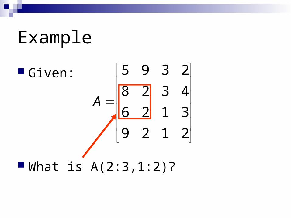
Example

Given:

What is A(2:3,1:2)?

2129

3126

4328

2395

A

Review of Matrix Algebra Dot Product Matrix Multiplication Matrix Inverse Solutions to Systems of Linear Equations Solutions Using Matrix Inverse Solutions Using Matrix Left Division

Dot Products

The dot product is the sum of the products of corresponding elements in two vectors.

Dot product = A*B = Matlab Commands (either will work)

sum(A.*B)dot(A,B)

n

iiiba

1

Matrix Multiplication

A = [1 2 3; 0 1 0], B = [2 1; 0 0; 1 2] C = A*B c(1,1) = 1(2) + 2(0) + 3(1) = 5

N

kkjikji bac

1,

1 2 3

0 1 0

2 1

0 0

1 2

* =5 7

0 0

What Size Matrices Multiply? Write the matrix dimensions in normal form: (A_rows, A_columns) (B_rows, B_columns)

(3,4)(4,16) -> (3,16) (2,12)(12,19)->(2,19)

If the inside values are the same, the matricescan be multiplied. They are conformable formultiplication.

The result willhave this size.

rows

columns

The Identity Matrix and Powers

Let I bet the identity matrix For any matrix X, X*I = X = I*X I = [1 0 0; 0 1 0; 0 0 1], for a 3x3 matrix In general I can be any square size with the

diagonal elements = 1, all others = 0

To multiply a matrix by itself, use X^2, or, in general, X^n

Inverse Matrices

Let A-1 be the inverse matrix of A Then, A-1A = AA-1 = I

Before computers, finding inverses was a pain in the neck

Not all matrices have inverses

2 1 1.5 0.5 1 0

4 3 2 1 0 1

Determinants

Most of the techniques to find inverses, and many other techniques that use matrices, at some point or other require determinants. These are special functions performed on matrices

If A is a 2x2 matrix, then the determinant is:Det(A) = a(1,1)*a(2,2) – a(1,2)*a(2,1)

Determinants for 3x3 Matrices A [ 1 2 3; 4 5 6; 7 8 9] Det(A) = + a(1,1)*(a(2,2)*a(3,3) – a(2,3)*a(3,2)) - a(1,2)*(a(2,1)*a(3,3) – a(2,3)*a(3,2)) + a(1,3)*(a(2,1)*a(3,2) - a(2,2)*a(3,1))

1 0 2

1 2 1

2 0 1

=2 -0 -8=-6

Solution of Linear Equations Perhaps the best thing about matrices is

how well they deal with systems of simultaneous linear equations

3x +2y -z = 10

-x +3y +2z = 5

x -y -z = -1

3 2 -1

-1 3 2

1 -1 -1

x

y

z

=*

10

5

-1

A*X = B

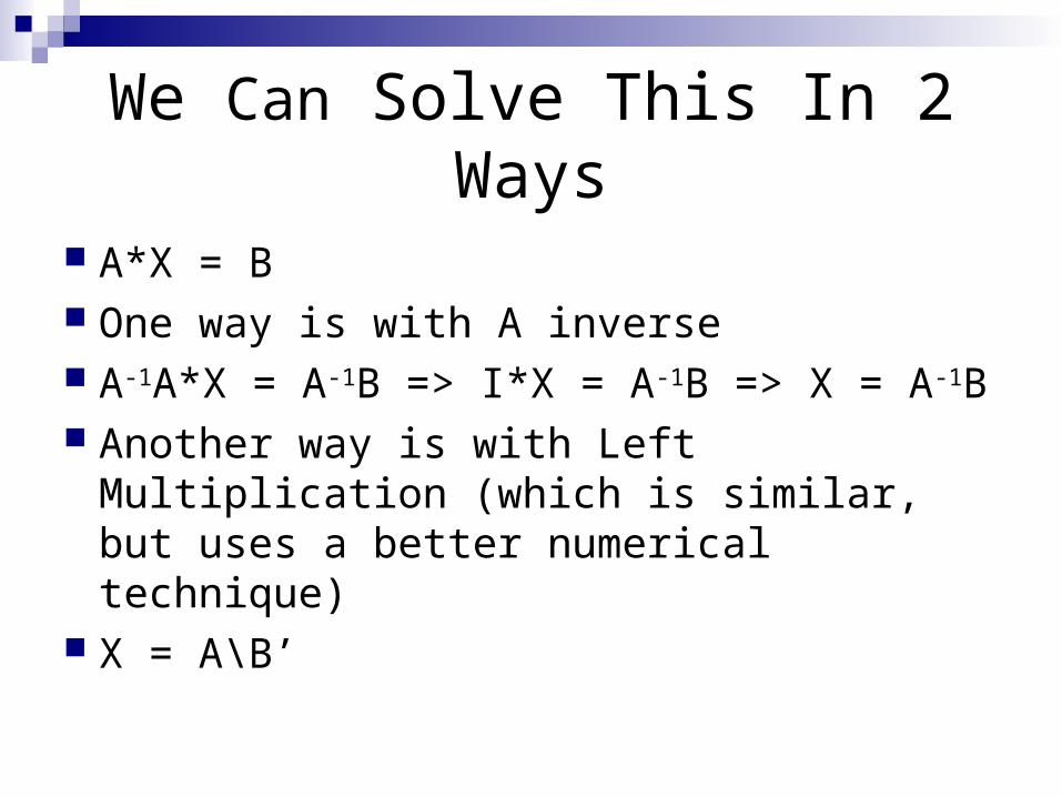
We Can Solve This In 2 Ways

A*X = B One way is with A inverse A-1A*X = A-1B => I*X = A-1B => X = A-1B Another way is with Left Multiplication

(which is similar, but uses a better numerical technique)

X = A\B’

Why Do Some Matrices Not Have Inverses?

X +2y = 0

X +2y = 0A =

1 2

1 2

X = -2y,No solution

X +2y = 0

2X +4y = 0A =

1 2

2 4

X = -2y,No solution

An Example

x1 – x2 – x3 – x4 = 5

x1 + 2x2 + 3x3 + x4 = -2

2x1 + 2x3 + 3x4 = 3

3x1 + x2 + 2x4 = 1

A = [1 –1 –1 –1;1 2 3 1; 2 0 2 3; 3 1 0 2]B = [5 –2 3 1]

X = inv(A)*B’ or X = A\B’

Some Useful Matrix Commands

Command Description

mean(b) Finds average of each column of b

max(b) Finds max of each column of b

min(b) Finds min of each column of b

sort(b) Sorts each column in b, ascending

sum(b) Sums each column in b

If A = 5 9 3 2

8 2 3 4

6 2 1 3

9 2 1 2

B = mean(A) = 7.0 3.75 2.0 3.75

C = max(A) = 9 9 3 4

D = min(A) = 5 2 1 2

E = sum(A) = 28 15 8 11

If A = 5 9 3 28 2 3 46 2 1 39 2 1 2

S = sort(A) = 5 2 1 26 2 1 28 2 3 39 9 3 4

Plotting

Plotting Basics

2D Plots (x,y)y=f(x)plot(x,y)

3D Plots (x,y,z): a.k.a. “surface plots”plot3(x,y,z)

Basic Commands

plot(x,y) xlabel(‘Distance (miles)’) ylabel(‘Height (miles)’) title(‘Rocket Height as a Function of Downrange distance’)

grid axis([0 10 0 100]) clf % clear current figure

Subplots

Subplotssubplot(m,n,p)

m = the number of figure rows n = the number of figure columns

Divides figure window into an array of rectangular frames

Comparing data plotted with different axis types

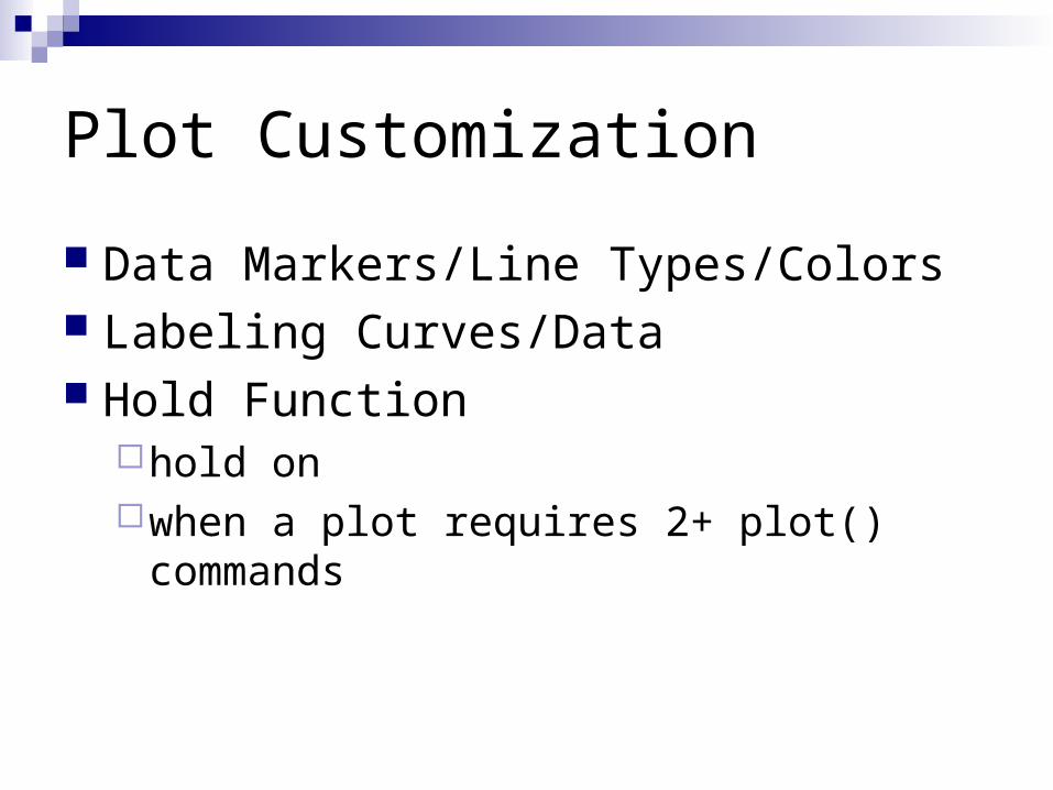
Plot Customization

Data Markers/Line Types/Colors Labeling Curves/Data Hold Function

hold onwhen a plot requires 2+ plot() commands

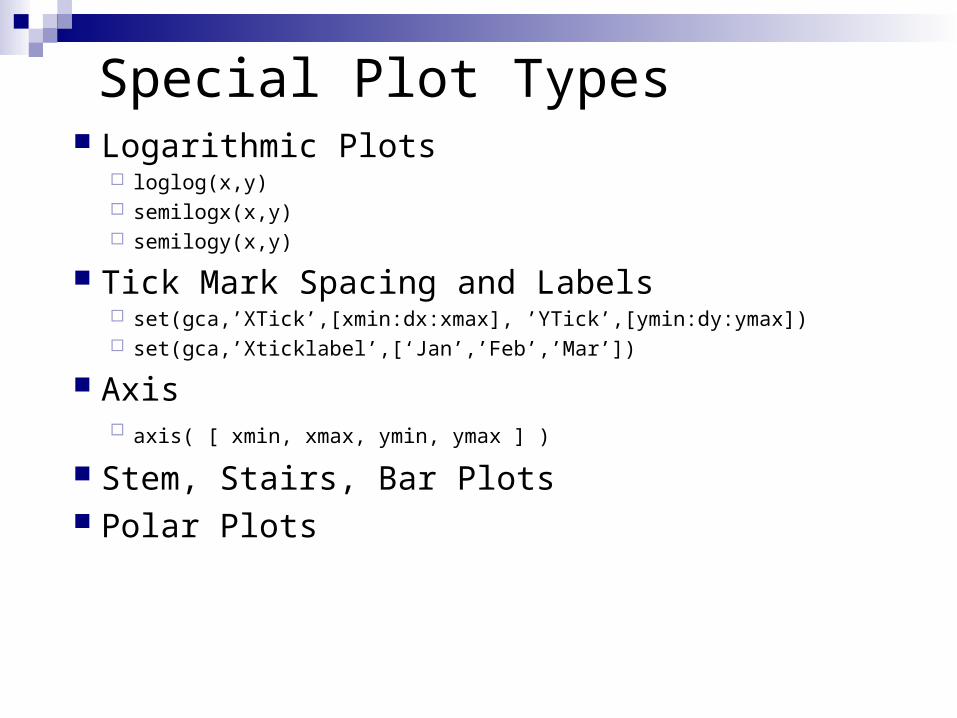
Special Plot Types Logarithmic Plots

loglog(x,y) semilogx(x,y) semilogy(x,y)

Tick Mark Spacing and Labels set(gca,’XTick’,[xmin:dx:xmax], ’YTick’,[ymin:dy:ymax]) set(gca,’Xticklabel’,[‘Jan’,’Feb’,’Mar’])

Axis axis( [ xmin, xmax, ymin, ymax ] )

Stem, Stairs, Bar Plots Polar Plots

Plot bells & whistlesVarious line types, plot symbols and colors may be obtained with PLOT(X,Y,S) where S is a character string from any or all the following 3 columns:

S = ‘ linetype color shape of data annotation ‘

Colors Data symbol Line type b blue . point - solidg green o circle : dottedr red x x-mark -. dashdot c cyan + plus -- dashed m magenta * stary yellow s squarek black d diamond v triangle (down) ^ triangle (up) < triangle (left) > triangle (right) p pentagram h hexagram

Plot(X,Y,S) examples

PLOT(X,Y,'c+:') plots a cyan dotted line with a plus at each data point

PLOT(X,Y,'bd') plots blue diamond at each data point but does not draw any line.

PLOT(X1,Y1,S1,X2,Y2,S2,X3,Y3,S3,...) combines the plots defined by the (X,Y,S) triples, where the X's and Y's are vectors or matrices and the S's are strings. For example, PLOT(X,Y,'y-',X,Y,'go') plots the data twice, with a solid yellow line interpolating green circles at the data points.

Function Discovery

The process of determining a function that can describe a particular set of dataLINEARPOWEREXPONENTIAL

polyfit() command

3D Plots

3D Line Plots plot3(x,y,z)

Surface Mesh Plots meshgrid() mesh(), meshc() surf(), surfc()

Contour Plots meshgrid() contour()

Data m-file

y = 1:5;

x = 1:12;

for i = 1:5

for j = 1:12

z(i,j) = i^1.25 * j ;

end;

end;

datax = 1 2 3 4 5 6 7 8 9 10 11 12

y = 1 2 3 4 5

z =

1.0000 2.0000 3.0000 4.0000 5.0000 6.0000 7.0000

2.3784 4.7568 7.1352 9.5137 11.892 14.270 16.6489

3.9482 7.8964 11.844 15.792 19.741 23.689 27.6376

5.6569 11.313 16.970 22.627 28.284 33.941 39.5980

7.4767 14.953 22.430 29.907 37.383 44.860 52.3372

Columns 8 through 12

8.000 9.000 10.000 11.000 12.000

19.02 21.405 23.784 26.162 28.541

31.58 35.534 39.482 43.430 47.378

45.25 50.911 56.568 62.225 67.882

59.81 67.290 74.767 82.244 89.720

3-D demo m-filesurf(x,y,z)

pause

mesh(x,y,z)

pause

waterfall(x,y,z)

pause

waterfall(y,x,z’)

pause

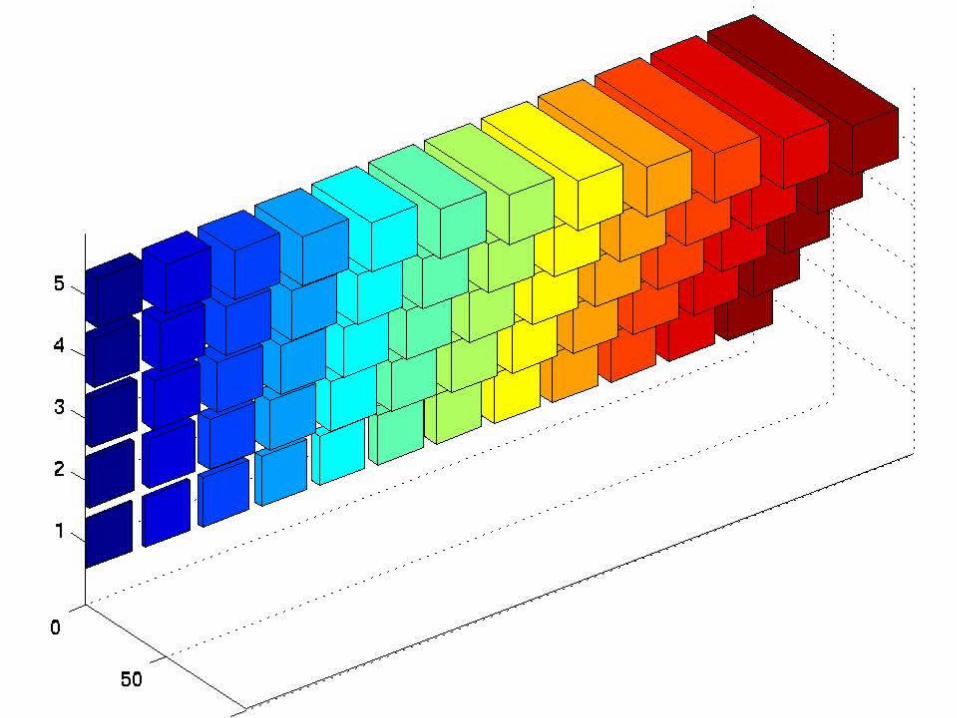
bar3(y,z)

pause

bar3h(y,z)

Reduced mesh

waterfall(x,y,z)

waterfall(y,x,z')

Title:Wat_fallA.epsCreator:MATLAB, The Mathworks, Inc.Preview:This EPS picture was not savedwith a preview included in it.Comment:This EPS picture will print to aPostScript printer, but not toother types of printers.