Epilepsy EEG classification using morphological component ...

RESEARCH Open Access

Epilepsy EEG classification usingmorphological component analysisArindam Gajendra Mahapatra1* , Balbir Singh1,2, Hiroaki Wagatsuma1,3,4 and Keiichi Horio1

Abstract

In this paper, we have proposed an application of sparse-based morphological component analysis (MCA) to addressthe problem of classification of the epileptic seizure using time series electroencephalogram (EEG). MCA was employedto decompose the EEG signal segments considering its morphology during epileptic events using undecimatedwavelet transform (UDWT), local discrete cosine transform (LDCT), and Dirac bases forming the over-completedictionary. Frequency-modulated time frequency features were extracted after applying the Hilbert transform. Featureroot mean instantaneous frequency square (RMIFS) and its parameters and parameters ratio are used in two differentpairs for classification using support vector machine (SVM), showing good and comparable results.

Keywords: Electroencephalogram (EEG), Morphological component analysis (MCA), Undecimated wavelet transform(UDWT), Local discrete cosine transform (LDCT), Dirac, Root mean instantaneous frequency square (RMIFS), Supportvector machine (SVM)

1 IntroductionHyperactivity of neural subnetwork resulting into dys-functioning of the brain from few seconds to several mi-nutes can be considered as epileptic seizure [1]. Epilepticseizure has broad classification based on various causesand symptoms or signs [2]. EEG have been used for earlydiagnosis and detection of seizures. It carries valuablecomplex information of brain activity. Manual inspec-tion of patient’s EEG is time consuming, and secondly, itis not accurate. Therefore, seizure diagnosis and detec-tion system discriminating seizure data from nonseizureand interictal EEG providing information about data fordiagnosis come handy. Seizure detection or classificationsystem mainly consists of two parts. First, preprocessing,filter or decompose the EEG for feature computationand extraction, and second, use these data from the firstpart for the classification by some supervised algorithm[3]. This decomposition process and feature extractionin the first part plays a pivotal role. As EEG is a graph-ical representation of summation of neuronal activity re-corded using electrodes over the scalp. It is important todecompose it into oscillatory modes risen from different

brain activity. Seizure detection requires good featuresshowing prominent difference for different brain activity.Classification of seizure against nonseizure healthy EEGhelps in diagnosis of epileptic seizure occurrence in thesubject, whereas classification of epileptic seizure (ictal)from interictal (the period between two consecutive sei-zures) is important for seizure warning and detectionsystem [4]. In the past, various methods have been pro-posed and developed for seizure classification based onfrequency domain such as Fourier [5, 6]. Short-timeFourier transform (STFT) methods based ontime-frequency methods were also used [7] for this pur-pose. In STFT, window size is a crucial factor for decid-ing the tradeoff between frequency and time resolution[8]. Utilizing wavelet analysis [8, 9] and its variant likediscrete wavelet transform for classification as employedby Guo et al. [10] to pre-analyze the EEG signals for epi-lepsy. Chen et al. [11] did similar work using dual treecomplex wavelet (DTCWT) for decomposition to extractfeature based on the logarithm of fast Fourier transform(FFT). Nearest neighbor (NN) classifier was used uponextracted features.Various machine learning techniques have been used

in conjunction with feature extraction for the classifica-tion of ictal from interictal and healthy nonseizure EEG.Feature extraction is an important part of this process

* Correspondence: [email protected] School of Life Science and Systems Engineering, Kyushu Instituteof Technology, Kitakyushu, JapanFull list of author information is available at the end of the article

EURASIP Journal on Advancesin Signal Processing

© The Author(s). 2018 Open Access This article is distributed under the terms of the Creative Commons Attribution 4.0International License (http://creativecommons.org/licenses/by/4.0/), which permits unrestricted use, distribution, andreproduction in any medium, provided you give appropriate credit to the original author(s) and the source, provide a link tothe Creative Commons license, and indicate if changes were made.

Mahapatra et al. EURASIP Journal on Advances in Signal Processing (2018) 2018:52 https://doi.org/10.1186/s13634-018-0568-2

http://crossmark.crossref.org/dialog/?doi=10.1186/s13634-018-0568-2&domain=pdf

http://orcid.org/0000-0002-8852-2297

mailto:[email protected]

http://creativecommons.org/licenses/by/4.0/

and influence the discrimination power of the model[12]. Features like approximate entropy (ApEn) withautoregressive model and principal component analysis(PCA) were applied by Liang et al. [4]. K nearest neigh-bor (KNN), support vector machine (SVM), least squaresupport vector machine (LS-SVM), decision trees, andnaive Bayes are used on features derived fromcross-correlation and power spectral density of signals[13, 14]. Genetic algorithm was used by Guo et al. [10]for feature extraction and classification purpose fromfeature database created by using discrete wavelet trans-form. SVM assembly implementation using median Tea-ger energy and Limpel-Ziv entropy feature from fivedifferent frequency sub-bands computed from band-passGabor filter bank is presented in [15]. Permutation en-tropy feature was used in [16] to create seizure detectionsystem. Complex network based ictal classification doneby Zhu et al. [17]. Tempko et al. [18] had used a total of55 features from time, frequency, energy, and entropydomain for classification of epileptic seizure.Empirical mode decomposition (EMD) by Huang et al.

[19] was used for EEG decomposition and feature compu-tation and extraction for epilepsy classification. Featureslike weighted frequency [20], standard deviation, mean,variance, skew, and centroid [21, 22] are extracted usingEMD for classification. Bandwidth based features from in-trinsic mode functions (IMFs) of EMD were fed toLS-SVM in [23]. RMS frequency feature extracted fromIMFs used upon SVM for classification of seizure was pre-sented in [24]. Phase space representation in Sharma et al.[25] was utilized for discrimination of ictal has also showngood results. Sparse-based decomposition [26] and classi-fication [27] are also proposed lately.In epilepsy, the commonly observed behavior or

morphology is spike train and sharp waves. The suddentransient burst of spikes and high-frequency oscillationsin interictal recordings are also used for the localizationof the epileptic seizures. Both disparity in backgroundactivity and EEG paroxysms make the automated ana-lysis complicated. Artifacts in filtered data can give riseto false positives [28–30]. Recently, signal decompositionby focusing on morphological components are gettinghighlighted due to its applicability to nonlinear andnon-stationary signal properties [31–33]. The mixing ofsources causes the EEG signal to be nonlinear andnon-stationary in nature. Due to this, separation ofsources from desired mixed signal become more difficultin time or frequency domain. MCA uses the linear com-bination of coefficients similar to independent compo-nent analysis (ICA). PCA and ICA [34] are popularmethods used for separation of sources or removal of ar-tifacts. Both the methods works on a statistical approachand aim to find the linear projection of the signals, i.e.,statistically independent [34]. The subspace projection is

used to extract EEG components on time/space basis.PCA is a sophisticated method to reduce the artifacts andspecifies principal components (PC) to reconstruct overalldata structure and to remove the components with smallamplitudes and irregular changes. It is very difficult tospecify remaining PCs to represent such signal. Toidentify PC requires the prior knowledge of the artifacts[35]. In ICA, different estimation procedures such asmutual information minimization, maximization ofnon-Gaussianity, maximization of likelihood, SOBI, andFastica are used for separation. Since ICA is based on themeasure of statistical independence, the noise of the inputis amplified by ICA and it makes the detection of the sig-nal components difficult due to Gaussian noise spreadover the component in an undesired way [36]. ICA gener-ates spikes and bumps, if the sample size is not sufficient[37, 38]. Basic ICA is a multichannel source separationtechnique and does not work on single channel unlikeMCA which can work perfectly with single channel [39].Although MCA is well known in image processing do-main [40, 41], it had found few applications in biomedicalsignal processing even after showing promising results inremoving artifacts from EEG [39, 42, 43]. MCA identifythe components of the signal based on sparsity in timefrequency domain. It decompose the signal and then ac-curately reconstruct the signal using redundant trans-forms (mathematical function) called explicit dictionary.This combination of explicit dictionary formingover-complete dictionary is important for representationof different morphologies of EEG signal. Sparse-based re-construction of EEG signal has an advantage of usingminimum coefficients which gives it the advantage to beeasily transferred it over the Internet. Every method hasadvantages and disadvantages and yet to reach the stagefor real-time analysis as a single method.The objective of this work is to present an approach con-

sidering the morphology of the EEG during an epilepticevent for diagnosing and detection of the epileptic seizure.In this work, we have used MCA with undecimated wavelettransform (UDWT), local discrete cosine transform(LDCT), and Dirac bases composing the dictionary for de-composition. UDWT identifies the slow components in theEEG, LDCT identifies the spectral components, and Diracidentifies the spikes in the EEG. Root mean instantaneousfrequency square (RMIFS) and the ratio of its consisting pa-rameters from Dirac component are computed and givento SVM as input for classification. RMIFS is defined assquare root over the sum of the time average squared band-width σ2T and the center frequency square <ω>2. These twoparameters, σ2T extracted from Dirac component and <ω>2

from LDCT component, are also used for classification.These two sets of features show considerable high accuracyand sensitivity comparable with other existing works.

Mahapatra et al. EURASIP Journal on Advances in Signal Processing (2018) 2018:52

of 12

This paper is organized as MCA followed by theHilbert transform, computation of feature, SVM, anddataset used followed by simulation and describing thephysical relevance of the features, then Section 9 andSection 10 at the end.

2 Method and materialIn the subsequent subsections, MCA is elaborated first,followed by features computed from its output decom-position. Briefly explained the SVM and the materialand the data used in this work.

3 Morphological component analysisMorphological component analysis uses the concept ofsparsity and independent redundant transforms to de-compose an EEG signal by adapting to the prevailingtypes of morphologies simultaneously. RepresentingEEG as a sparse linear contribution of coefficients, MCAuses over-complete dictionary Φ ∈ Rn × k, where k isthe morphological components of an EEG signal S ∈ Rn

decomposed by constructing source components {∅k}k ∈Γ, where Γ representing the type of explicit dictionaries.An EEG signal can be represented as a sparse linearcombination of coefficients. Over-complete dictionaryΦ is a set of explicit dictionary, defined by a set ofmathematical functions to represent the specific morph-ologies of EEG [44]. Signal can be represented as

S ¼Xk

i¼0βi∅i þ ζ ¼ β1∅1 þ β2∅2…þ βk∅k

þζ≅s1 þ s2…þ sk ζ≪1ð Þ ¼ S0

ð1Þwhere ∅k represents a set of basis elements and β is thetarget coefficients to reconstruct the original EEG signal.ζ is assumed to be negligible noise tend to zero. By usingthree dictionaries, undecimated wavelet transform(UDWT), local discrete cosine transform (LDCT), and

Dirac (Kronecker basis) [39, 45, 46] in this work, coeffi-cients are optimized as

fβopt0 ; βopt1 ; βopt2 g ¼ arg minβ0;⋯;β2

X2i¼0

∥βi∥0 ð2Þ

subject to S′ ¼ Pki¼0βi∅ i; k ¼ 2 in this work:

The basis pursuit solution [47] was used to representthe sparse component which describes Eq. (1) as

fβopt0 ; βopt1 ; βopt2 g ¼ arg minβ0;⋯;β2

X2i¼0

∥βi∥1

þ λ∥S−X2i¼0

∅ iβi∥2

2

ð3Þ

Equation (3) is optimized by block coordinate relax-ation (BCR) method [48] in finite time. The algorithmgiven in [39] is as follows:

The number of iteration Imax=100 is used. Balbir et al.[39] had varied the value of λ from 3 to 5 depending onthe type of hard and soft threshold. In this work, λ = 3 isused. Figure 1 depicts the working of MCA as described inAlgorithm 1. From Figs. 2 and 3, it can be observed that

Fig. 1 Block diagram of MCA decomposition of EEG signal


of 12

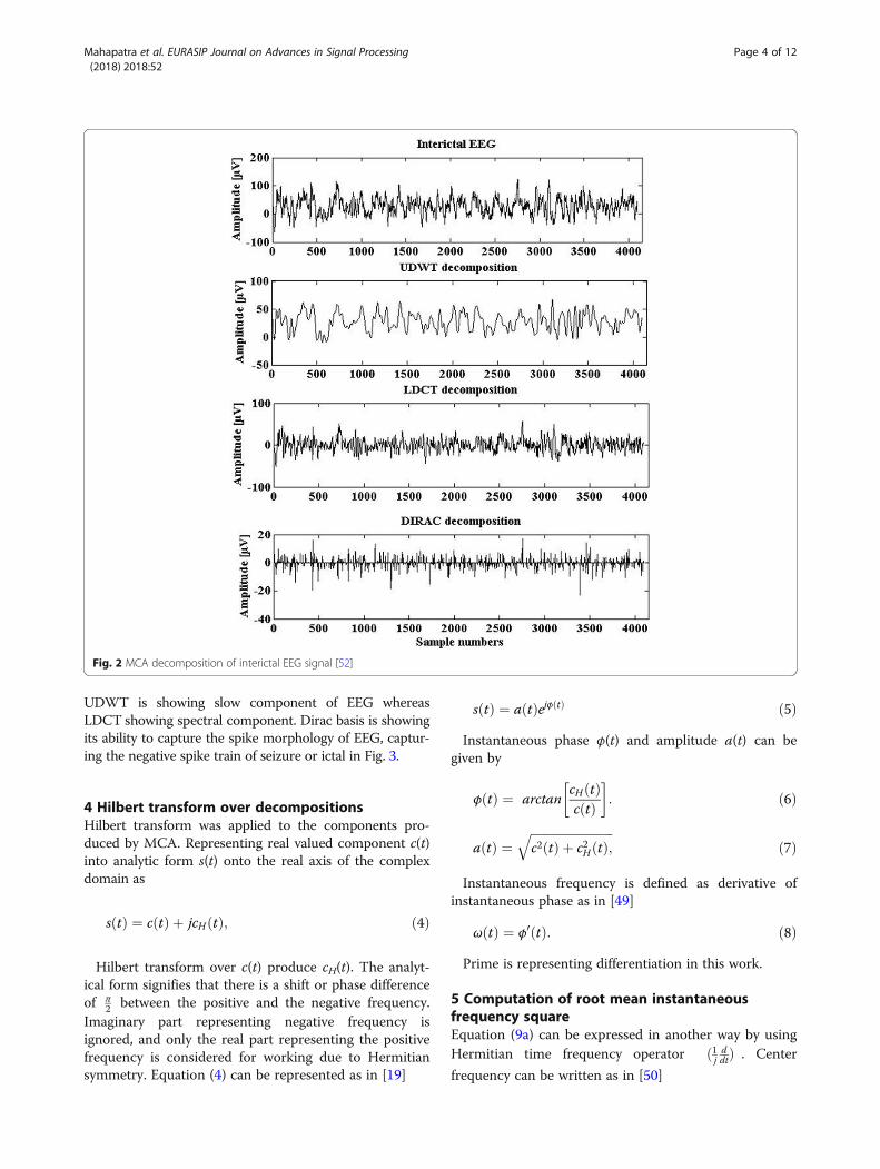
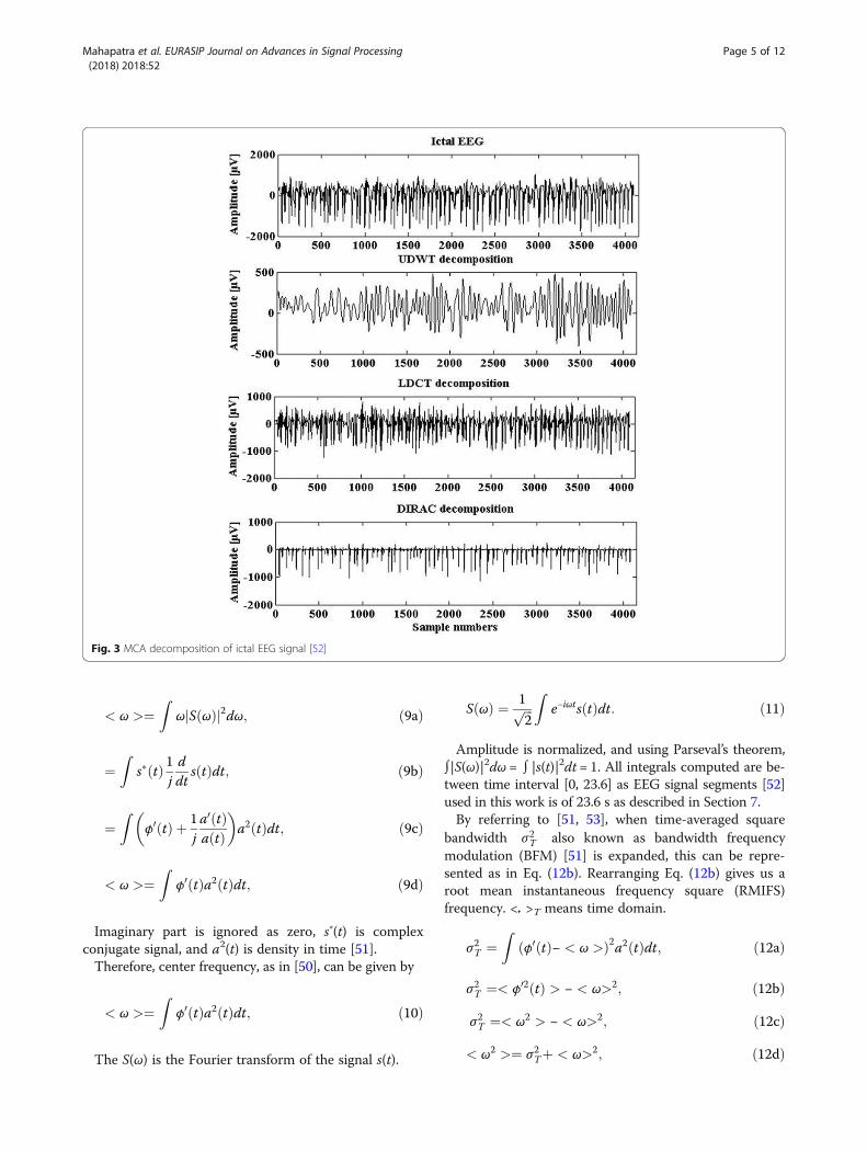
UDWT is showing slow component of EEG whereasLDCT showing spectral component. Dirac basis is showingits ability to capture the spike morphology of EEG, captur-ing the negative spike train of seizure or ictal in Fig. 3.

4 Hilbert transform over decompositionsHilbert transform was applied to the components pro-duced by MCA. Representing real valued component c(t)into analytic form s(t) onto the real axis of the complexdomain as

s tð Þ ¼ c tð Þ þ jcH tð Þ; ð4Þ

Hilbert transform over c(t) produce cH(t). The analyt-ical form signifies that there is a shift or phase differenceof π

2 between the positive and the negative frequency.Imaginary part representing negative frequency isignored, and only the real part representing the positivefrequency is considered for working due to Hermitiansymmetry. Equation (4) can be represented as in [19]

s tð Þ ¼ a tð Þejφ tð Þ ð5ÞInstantaneous phase φ(t) and amplitude a(t) can be

given by

φ tð Þ ¼ arctancH tð Þc tð Þ

� �: ð6Þ

a tð Þ ¼ffiffiffiffiffiffiffiffiffiffiffiffiffiffiffiffiffiffiffiffiffiffiffiffiffiffiffic2 tð Þ þ c2H tð Þ;

qð7Þ

Instantaneous frequency is defined as derivative ofinstantaneous phase as in [49]

ω tð Þ ¼ φ0 tð Þ: ð8ÞPrime is representing differentiation in this work.

5 Computation of root mean instantaneousfrequency squareEquation (9a) can be expressed in another way by usingHermitian time frequency operator ð1j ddtÞ . Center

frequency can be written as in [50]

Fig. 2 MCA decomposition of interictal EEG signal [52]


of 12

< ω >¼Z

ω S ωð Þj j2dω; ð9aÞ

¼Z

s� tð Þ 1jddt

s tð Þdt; ð9bÞ

¼Z

φ0 tð Þ þ 1ja0 tð Þa tð Þ

� �a2 tð Þdt; ð9cÞ

< ω >¼Z

φ0 tð Þa2 tð Þdt; ð9dÞ

Imaginary part is ignored as zero, s∗(t) is complexconjugate signal, and a2(t) is density in time [51].Therefore, center frequency, as in [50], can be given by

< ω >¼Z

φ0 tð Þa2 tð Þdt; ð10Þ

The S(ω) is the Fourier transform of the signal s(t).

S ωð Þ ¼ 1ffiffiffi2

pZ

e−iωts tð Þdt: ð11Þ

Amplitude is normalized, and using Parseval’s theorem,∫|S(ω)|2dω = ∫ |s(t)|2dt = 1. All integrals computed are be-tween time interval [0, 23.6] as EEG signal segments [52]used in this work is of 23.6 s as described in Section 7.By referring to [51, 53], when time-averaged square

bandwidth σ2T also known as bandwidth frequencymodulation (BFM) [51] is expanded, this can be repre-sented as in Eq. (12b). Rearranging Eq. (12b) gives us aroot mean instantaneous frequency square (RMIFS)frequency. <. >T means time domain.

σ2T ¼Z

φ0 tð Þ− < ω >ð Þ2a2 tð Þdt; ð12aÞ

σ2T ¼< φ02 tð Þ > − < ω>2; ð12bÞ

σ2T ¼< ω2 > − < ω>2; ð12cÞ

< ω2 >¼ σ2Tþ < ω>2; ð12dÞ

Fig. 3 MCA decomposition of ictal EEG signal [52]


of 12

f R ¼ffiffiffiffiffiffiffiffiffiffiffiffiffiffiffiffiffiffiffiffiffiffiffiffiffiσ2Tþ < ω>2

q: ð12eÞ

σ2T and <ω>2 are parameters, as can be seen in Eq.(12d), and their ratio can be given by

EMIFS ¼ < ω>2

σ2T

: ð13Þ

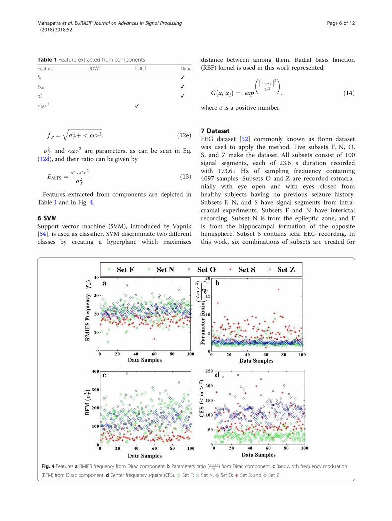
Features extracted from components are depicted inTable 1 and in Fig. 4.

6 SVMSupport vector machine (SVM), introduced by Vapnik[54], is used as classifier. SVM discriminate two differentclasses by creating a hyperplane which maximizes

distance between among them. Radial basis function(RBF) kernel is used in this work represented:

G xi; x j� � ¼ exp

xi ;−x jk k2

2σ2

� �; ð14Þ

where σ is a positive number.

7 DatasetEEG dataset [52] commonly known as Bonn datasetwas used to apply the method. Five subsets F, N, O,S, and Z make the dataset. All subsets consist of 100signal segments, each of 23.6 s duration recordedwith 173.61 Hz of sampling frequency containing4097 samples. Subsets O and Z are recorded extracra-nially with eye open and with eyes closed fromhealthy subjects having no previous seizure history.Subsets F, N, and S have signal segments from intra-cranial experiments. Subsets F and N have interictalrecording. Subset N is from the epileptic zone, and Fis from the hippocampal formation of the oppositehemisphere. Subset S contains ictal EEG recording. Inthis work, six combinations of subsets are created for

Table 1 Feature extracted from components

Feature UDWT LDCT Dirac

fR ✓

EMIFS ✓

σ2T ✓

<ω>2 ✓

Fig. 4 Features a RMIFS frequency from Dirac component. b Parameters ratio (<ω>2

σ2T) from Dirac component. c Bandwidth frequency modulation

(BFM) from Dirac component. d Center frequency square (CFS). Set F; Set N; Set O; Set S; and Set Z


of 12

classification. First one is with sets F, S, second withN, S, third with O against S, fourth with Z against S,fifth with F, N together versus S, and sixth with O, Zagainst S for classification.Every subset contains 100 data from each feature

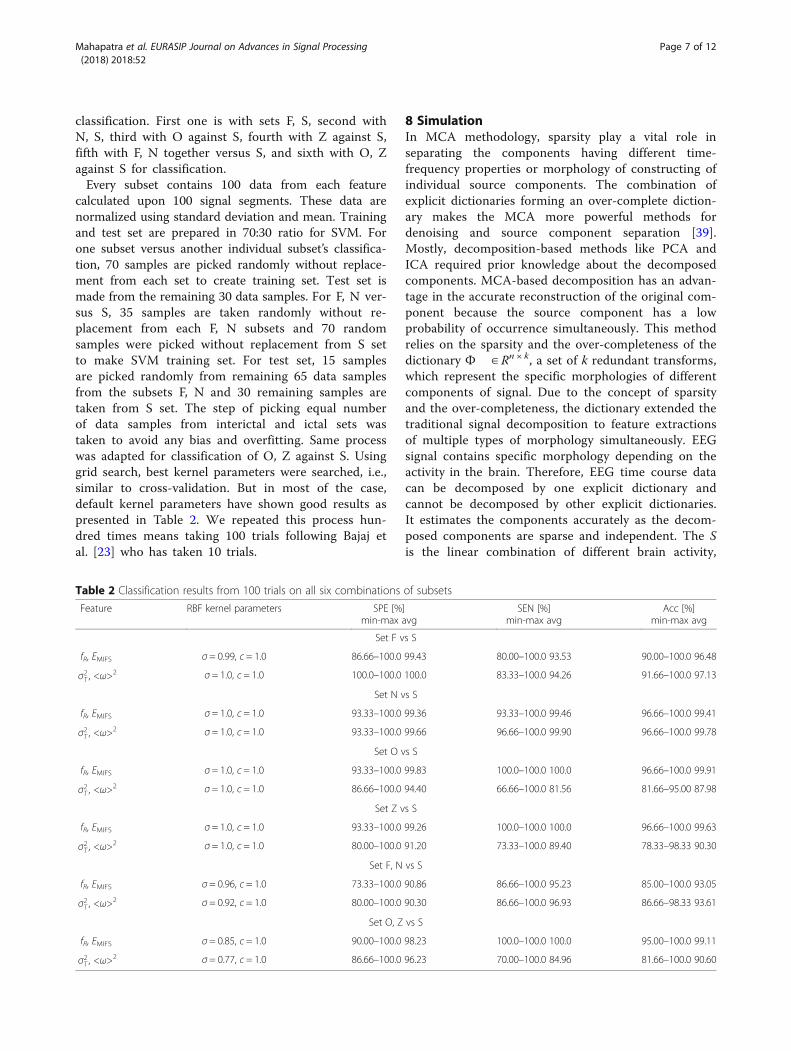
calculated upon 100 signal segments. These data arenormalized using standard deviation and mean. Trainingand test set are prepared in 70:30 ratio for SVM. Forone subset versus another individual subset’s classifica-tion, 70 samples are picked randomly without replace-ment from each set to create training set. Test set ismade from the remaining 30 data samples. For F, N ver-sus S, 35 samples are taken randomly without re-placement from each F, N subsets and 70 randomsamples were picked without replacement from S setto make SVM training set. For test set, 15 samplesare picked randomly from remaining 65 data samplesfrom the subsets F, N and 30 remaining samples aretaken from S set. The step of picking equal numberof data samples from interictal and ictal sets wastaken to avoid any bias and overfitting. Same processwas adapted for classification of O, Z against S. Usinggrid search, best kernel parameters were searched, i.e.,similar to cross-validation. But in most of the case,default kernel parameters have shown good results aspresented in Table 2. We repeated this process hun-dred times means taking 100 trials following Bajaj etal. [23] who has taken 10 trials.

8 SimulationIn MCA methodology, sparsity play a vital role inseparating the components having different time-frequency properties or morphology of constructing ofindividual source components. The combination ofexplicit dictionaries forming an over-complete diction-ary makes the MCA more powerful methods fordenoising and source component separation [39].Mostly, decomposition-based methods like PCA andICA required prior knowledge about the decomposedcomponents. MCA-based decomposition has an advan-tage in the accurate reconstruction of the original com-ponent because the source component has a lowprobability of occurrence simultaneously. This methodrelies on the sparsity and the over-completeness of thedictionary Φ ∈ Rn × k, a set of k redundant transforms,which represent the specific morphologies of differentcomponents of signal. Due to the concept of sparsityand the over-completeness, the dictionary extended thetraditional signal decomposition to feature extractionsof multiple types of morphology simultaneously. EEGsignal contains specific morphology depending on theactivity in the brain. Therefore, EEG time course datacan be decomposed by one explicit dictionary andcannot be decomposed by other explicit dictionaries.It estimates the components accurately as the decom-posed components are sparse and independent. The Sis the linear combination of different brain activity,

Table 2 Classification results from 100 trials on all six combinations of subsets

Feature RBF kernel parameters SPE [%]min-max avg

SEN [%]min-max avg

Acc [%]min-max avg

Set F vs S

fR, EMIFS σ = 0.99, c = 1.0 86.66–100.0 99.43 80.00–100.0 93.53 90.00–100.0 96.48

σ2T , <ω>2 σ = 1.0, c = 1.0 100.0–100.0 100.0 83.33–100.0 94.26 91.66–100.0 97.13

Set N vs S

fR, EMIFS σ = 1.0, c = 1.0 93.33–100.0 99.36 93.33–100.0 99.46 96.66–100.0 99.41

σ2T , <ω>2 σ = 1.0, c = 1.0 93.33–100.0 99.66 96.66–100.0 99.90 96.66–100.0 99.78

Set O vs S

fR, EMIFS σ = 1.0, c = 1.0 93.33–100.0 99.83 100.0–100.0 100.0 96.66–100.0 99.91

σ2T , <ω>2 σ = 1.0, c = 1.0 86.66–100.0 94.40 66.66–100.0 81.56 81.66–95.00 87.98

Set Z vs S

fR, EMIFS σ = 1.0, c = 1.0 93.33–100.0 99.26 100.0–100.0 100.0 96.66–100.0 99.63

σ2T , <ω>2 σ = 1.0, c = 1.0 80.00–100.0 91.20 73.33–100.0 89.40 78.33–98.33 90.30

Set F, N vs S

fR, EMIFS σ = 0.96, c = 1.0 73.33–100.0 90.86 86.66–100.0 95.23 85.00–100.0 93.05

σ2T , <ω>2 σ = 0.92, c = 1.0 80.00–100.0 90.30 86.66–100.0 96.93 86.66–98.33 93.61

Set O, Z vs S

fR, EMIFS σ = 0.85, c = 1.0 90.00–100.0 98.23 100.0–100.0 100.0 95.00–100.0 99.11

σ2T , <ω>2 σ = 0.77, c = 1.0 86.66–100.0 96.23 70.00–100.0 84.96 81.66–100.0 90.60


of 12

where β is the brain activity and is the mixingmatrix. Different basis functions were trialed in differ-ent combinations to create the epileptic-specific dic-tionary from a set of UDWT, discrete sine transform(DST), discrete cosine transform (DCT), LDCT, andDirac basis functions, and finally, UDWT, LDCT, andDirac were used depending on the significant differ-ence shown by the extracted, proposed features.UDWT has not been used directly for feature extrac-tion but has been kept in the dictionary to makeLDCT spectral component remain free fromslow-moving components. Dirac basis was used tocapture the spike morphology of the epileptic seizure.Dirac basis is also useful in capturing the transientspikes in interictal which can help in localizing theepileptic zone.After using MCA for decomposition, Hilbert trans-

form was applied over the components which take thereal value signal decomposition to complex time fre-quency domain. Real signal gives symmetrical density infrequency making mean or center frequency zero. Usinganalytic representation, we will have identical spectrumfor positive frequencies and zero for negative frequencies

[50]. Feature RMIFS (fR) and the parameters ratio (<ω>2

σ2T)

are computed from Dirac component. RMIFS is definedas root over sum of the time-averaged bandwidth squareσ2T and the center frequency square <ω>2. f 2R is alwaysgreater than <ω>2 by σ2T . This feature is expressed com-pletely in terms of frequency modulation σ2

T and averageor center frequency square <ω>2 in time domain whichis advantageous as it is free from any amplitude-basedcomponent that is prone to noise. Computing fR directly

asffiffiffiffiffiffiffiffiffiffiffiffiffiffiffiffiffiffiffiffiffiffi< φ02ðtÞ >p

or asffiffiffiffiffiffiffiffiffiffiffiffiffiffiffiffiffiffiffiffiffiffiffiffiffiσ2Tþ < ω>2

pgives same value.

The parameters ratio (<ω>2

σ2T) shows how dominant center

frequency square is over time-averaged bandwidthsquare. For example, from Fig. 4c, in the case of interic-tal σ2T is at higher range making the parameters ratio atlower range whereas for ictal the behavior is oppositemeans during the ictal event, the frequency modulationis small compared to interictal as also observed by Bajajet al. [23]. Frequency modulation σ2T from Dirac compo-nent is at higher range in nonseizure and interictal thanictal, and center frequency from LDCT component ishighest in nonseizure than in ictal and lowest in interic-tal. As time-averaged bandwidth can be taken as thestandard deviation of instantaneous frequency aroundthe center frequency and center frequency as themean, fR satisfies the definition of root mean square.Value of fR will be close to center frequency when in-stantaneous frequencies are close to center frequencyleading to small σ2

T . That is, signal decomposition duringepileptic event showing small frequency modulation will

result in f 2R influenced by center frequency square <ω>2.Dirac component was chosen for computation of RMIFSfrequency because, firstly, it represents the spike morph-ology of the EEG and, secondly, it shows more signifi-cant difference than when fR is computed from LDCT

component. For classification using <ω>2 and σ2T , <ω>

2

is computed from LDCT component and σ2T from Dirac

component simultaneously because LDCT representsthe frequency component better than Dirac which showsmodulation better.Center frequency square <ω>2 calculated from LDCT

component are in range from higher delta wave to loweralpha wave in interictal sets F, N, whereas in healthynonseizure sets O, Z, it is between higher theta wave toalpha wave. Center frequency in ictal set S was dispersedbetween lower theta wave to lower beta wave. RMIFS fRon an average is in beta range for all the subsets of theBonn dataset as presented in Fig. 4.

9 Results and discussionThese features are normalized using mean and standarddeviation then fed to SVM in a set of two pairs separ-ately to elaborate its significance in classification ofseizures. These pairs of features are selected as they areshowing opposite behavior which helps SVM to createthe hyperplane discriminating the classes. Performanceof the SVM classifier is evaluated by using the statisticalparameters from previous works, i.e., specificity (SPE),sensitivity (SEN), and accuracy (Acc) [4, 23].

SPE ¼ TNTNþ FP

� 100; ð15Þ

SEN ¼ TPTPþ FN

� 100; ð16Þ

Acc ¼ TPþ TNTPþ TNþ FPþ FN

� 100; ð17Þ

where true positive and true negative events are denotedby TP and TN, i.e., detecting ictal and interictal cor-rectly. FN and FP stands for false negative and false posi-tive, respectively.Classification of result of set F versus set S using both

pairs of feature, i.e., fR, (<ω>2

σ2T) and σ2T , <ω>

2 shows simi-

lar result of average accuracy of 96.48 and 97.13% andaverage sensitivity of 93.53 and 94.26%. Average specifi-city using both the features are very high at 99.43 and100.0%. Results are shown in Table 2.Classification accuracy of both the pairs of feature for

set N against S is good at 99.41 and 99.48%. Averagesensitivity and specificity are 99.46, 99.90, 99.36, and

99.66%. For set O versus Z, features fR, (<ω>2

σ2T) show aver-

age accuracy of 99.91%, but σ2T , <ω>

2 achieved lowly at


of 12

Fig. 5 Set N vs S classification using RBF kernel σ = 1.0, c = 1.0. 0 (Ictal Training); 1 (Interictal Training); Support Vectors; SVM Hyperplane;0 (Ictal Classified); and 1 (Interictal Classified)

Fig. 6 Set O vs S classification using RBF kernel σ = 1.0, c = 1.0. 0 (Ictal Training); 1 (NonSeizure Training); Support Vectors; SVMHyperplane; 0 (Ictal Classified); 1 (NonSeizure Classified)


of 12

87.98%. Similar accuracy result is observed for set Z ver-

sus S with 99.63% using fR, (<ω>2

σ2T), whereas 90.30% using

σ2T , <ω>

2. SVM plot for set N versus S using σ2T , <ω>2

and set O against S using fR, (<ω>2

σ2T) is shown in Figs. 5

and 6. Average accuracy for set F, N together versus setS are at 93.05 and 93.61% for both sets of features,whereas average classification accuracy for set O, Z ver-sus S are at 99.11 and 90.60%. We have compared thisproposed work with previous work at Tables 3 and 4.

For most of the time default kernel parameters provedto be better. Even with an optimized parameters that arefound with grid search, were close to default setting andshows little improvement of at most 1–1.5%. Therefore,the cases where we found improvement less than 1%,default setting or default kernel parameters were usedwhich helped in avoiding computing overload of kernelparameters search and makes the application more prac-tical. Both the pairs of features have shown similar clas-sification result for interictal set versus ictal or seizure

Table 3 Comparison of set F, N vs S results with other existing works on Bonn dataset

Author Preprocessing method Feature used Classifier Set Accuracy [%]

Liang et al. [4] Fast Fourier transform 16 spectral features SVM F vs S 98.74

Siuly et al. [13] Clustering 9 temporal features LS-SVM F vs S 93.91

N vs S 97.69

Riaz et al. [21] EMD 6 temporal and spectral features Decision trees F vs S 96.00

SVM F vs S 93.00

Samiee et al. [55] Rational DSTFT 5 time frequency features MLP F vs S 94.90

N vs S 98.50

Hassan et al. [56] CEEMDAN 6 spectral features Boosting F vs S 97.00

N vs S 100.0

SVM F vs S 93.00

N vs S 99.00

Proposed work MCA σ2T , <ω>2 SVM F vs S 97.13

N vs S 99.78

Sharma et al. [25] EMD 2D, 3D, PSR LS-SVM F, N vs S 98.67

Altunay et al. [57] L. P Filter Energy feature Threshold F, N vs S 94.00

Joshi et al. [58] FLP FLP energy, signal energy SVM F, N vs S 95.33

Pachori et al. [59] EMD SODP of IMF ANN F, N vs S 97.75

Proposed work MCA σ2T , <ω>2 SVM F, N vs S 93.61

RDSTFT rational discrete STFT, CEEMDAN complete ensemble empirical mode decomposition with adaptive noise, PSR phase space representation, L. P Filter linearprediction filter, FLP fractional linear prediction

Table 4 Comparison with other works on Bonn dataset for classification between healthy nonseizure set O, Z and seizure or ictal set S

Author Preprocessing method Feature used Classifier Set Accuracy [%]

Guo et al. [10] Genetic algorithm Curve length, standard deviation KNN Z vs S 99.20

Siuly et al. [13] Clustering 9 temporal features LS-SVM Z vs S 99.90

O vs S 96.30

Samiee et al. [55] Rational DSTFT 5 time frequency features MLP Z vs S 99.80

Hassan et al. [56] CEEMDAN 6 spectral features Boosting Z vs S 100.0

Rincon et al. [60] Wavelet transform Bag of words SVM Z vs S 99.85

Wavelet coefficient SVM Z vs S 100.0

Proposed work MCA fR, EMIFS SVM Z vs S 99.63

O vs S 99.91

Chen et al. [11] DTCWT Logarithm of FFT spectra NN Z, O vs S 100

Proposed work MCA fR, EMIFS SVM Z, O vs S 99.11

MLP multilayer perceptron


of 12

set whereas feature fR, (<ω>2

σ2T) has shown better results

for healthy nonseizure classification against seizure set.

Therefore, fR, (<ω>2

σ2T) features combination for classifica-

tion are found to better than σ2T , <ω>2. Figure 4 clearly

shows it is hard to have two-dimensional map helpingSVM to create hyperplane to separate nonseizure andseizure sets using feature combination of σ2T , <ω>

2 asthey are quite intermingled. Although classification ofseizure set which is the result of intracranial experimentagainst noninvasive extracranial nonseizure healthy EEGset is inappropriate, classification has been done forcomparison purpose of the proposed method with previ-ous works. Detailed comparison of the proposed workwith the previously done work on Bonn dataset is pre-sented in Tables 3 and 4.

10 ConclusionsMCA gives definite number of decomposition depend-ing on the number of set of basis used in over-complete dictionary. This dictionary can be formedbased on problem requirements. Selection of basisfunctions in the dictionary plays an important role increating problem-specific application. We found LDCTcomponent is best suited for spectral feature extraction,whereas Dirac bases are good in showing spike morph-ology of the EEG. Default setting of SVM kernel is suit-able for proposed feature combinations which makes itsuitable for practical application. To make the methodreliable, 100 random trials were taken on SVM. 99.78%of highest average accuracy was observed for classifica-tion of interictal set N against ictal set S, whereas99.91% of average accuracy was observed for classifica-tion of nonseizure set O against ictal set S. In future,we will try to form a dictionary to remove different arti-facts from EEG and will try to create seizure predictionsystem using MCA and proposed features with suitablebasis for long-term EEG signals.

AbbreviationsAcc: Accuracy; ApEn: Approximate entropy; BCR: Block coordinate relaxation;BFM: Bandwidth frequency modulation; CEEMDAN: Complete ensembleempirical mode decomposition with adaptive noise; CFS: Center frequencysquare; DCT: Discrete cosine transform; DST: Discrete sine transform;DTCWT: Dual tree complex wavelet; EEG: Electroencephalogram;EMD: Empirical mode decomposition; FFT: Fast Fourier transform;FLP: Fractional linear prediction; FN: False negative; FP: False positive;ICA: Independent component analysis; IMF: Intrinsic mode function; KNN: Knearest neighbor; L.P Filter: Linear prediction filter; LDCT: Local discretecosine transform; LS-SVM: Least square support vector machine;MCA: Morphological component analysis; MLP: Multilayer perceptron;NN: Nearest neighbor; PC: Principal component; PCA: Principal componentanalysis; PSR: Phase space representation; RBF: Radial basis function;RDSTFT: Rational discrete STFT; RMIFS: Root mean instantaneous frequencysquare; SEN: Sensitivity; SPE: Specificity; STFT: Short-time Fourier transform;SVM: Support vector machine; TN: True negative; TP: True positive;UDWT: Undecimated wavelet transform

Availability of data and materialsThe EEG dataset [52] used in this work is available at http://www.meb.unibonn.de/epileptologie/science/physik/EEGdata.html

Authors’ contributionsThe MCA code developed by Dr. BS under the supervision of Dr. HW is usedin this work. Selection of basis function to create dictionary for epilepticapplication, feature proposal and extraction, classification and result analysisis done by AGM under the supervision of Dr. KH. All authors read andapproved the final manuscript.

Ethics approval and consent to participateNot applicable.

Consent for publicationNot applicable.

Competing interestsThe authors declare that they have no competing interests.

Publisher’s NoteSpringer Nature remains neutral with regard to jurisdictional claims inpublished maps and institutional affiliations.

Author details1Graduate School of Life Science and Systems Engineering, Kyushu Instituteof Technology, Kitakyushu, Japan. 2National Institute for PhysiologicalSciences, Okazaki, Japan. 3Artificial Intelligence Research Center, NationalInstitute of Advanced Industrial Science and Technology, Tokyo, Japan.4Riken BSI, Wako, Japan.

Received: 18 January 2018 Accepted: 18 June 2018

References1. RS Fisher, WE Boas, W Blume, C Elger, P Genton, P Lee, J Engel, Epileptic

seizures and epilepsy: definitions proposed by the international leagueagainst epilepsy (ilae) and the international bureau for epilepsy (ibe).Epilepsia 46(4), 470–472 (2005)

2. AT Berg, SF Berkovic, MJ Brodie, J Buchhalter, JH Cross, WE Boas, JEngel, J French, TA Glauser, GW Mathern, et al., Revised terminologyand concepts for organization of seizures and epilepsies: report of theILAE commission on classification and terminology, 2005-2009. Epilepsia51(4), 676–685 (2010)

3. S Ramgopal, S Thome-Souza, M Jackson, NE Kadish, IS Fernandez, J Klehm,W Bosl, C Reinsberger, S Schachter, T Loddenkemper, Seizure detection,seizure prediction, and closed-loop warning systems in epilepsy. EpilepsyBehav. 37, 291–307 (2014)

4. SF Liang, HC Wang, WL Chang, Combination of EEG complexity andspectral analysis for epilepsy diagnosis and seizure detection. EURASIP J.Adv. Signal Process. 2010(1), 853434 (2010)

5. V Srinivasan, C Eswaran, N Sriraam, Artificial neural network based epilepticdetection using time-domain and frequency-domain features. J. Med. Syst.29(6), 647–660 (2005)

6. K Polat, S Günes, Classification of epileptiform EEG using a hybrid systembased on decision tree classifier and fast Fourier transform. Appl. Math.Comput. 187(2), 1017–1026 (2007)

7. AT Tzallas, MG Tsipouras, DI Fotiadis, Epileptic seizure detection in EEGsusing time-frequency analysis. IEEE Trans. Inf. Technol. Biomed. 13(5), 703–710 (2009)

8. H Adeli, Z Zhou, N Dadmehr, Analysis of EEG records in an epileptic patientusing wavelet transform. J. Neurosci. Methods 123(1), 69–87 (2003)

9. H Ocak, Optimal classification of epileptic seizures in EEG using waveletanalysis and genetic algorithm. Signal Process. 88(7), 1858–1867 (2008)

10. L Guo, D Rivero, J Dorado, AP CR Munteanu, Automatic feature extractionusing genetic programming: an application to epileptic EEG classification.Expert Syst. Appl. 38(8), 10425–10436 (2011)

11. G Chen, Automatic EEG seizure detection using dual-tree complex wavelet-Fourier features. Expert Syst. Appl. 41(5), 2391–2394 (2014)

12. BL WC Stacey, Technology insight: neuroengineering and epilepsy-designingdevices for seizure control. Nat. Clin. Pract. Neurol. 4(4), 190–201 (2008)


of 12

http://www.meb.unibonn.de/epileptologie/science/physik/EEGdata.html

http://www.meb.unibonn.de/epileptologie/science/physik/EEGdata.html

13. Y Li, PP Wen, et al., Clustering technique-based least square support vectormachine for EEG signal classification. Comput. Methods Prog. Biomed.104(3), 358–372 (2011)

14. Z Iscan, Z Dokur, T Demiralp, Classification of electroencephalogram signalswith combined time and frequency features. Expert Syst. Appl. 38(8),10499–10505 (2011)

15. Y Tang, D Durand, A tunable support vector machine assemblyclassifier for epileptic seizure detection. Expert Syst. Appl. 39(4), 3925–3938 (2012)

16. N Nicolaou, J Georgiou, Detection of epileptic electroencephalogram basedon permutation entropy and support vector machines. Expert Syst. Appl.39(1), 202–209 (2012)

17. G Zhu, Y Li, PP Wen, Epileptic seizure detection in EEGs signals using a fastweighted horizontal visibility algorithm. Comput. Methods Prog. Biomed.115(2), 64–75 (2014)

18. A Temko, E Thomas, W Marnane, G Lightbody, G Boylan, EEG-basedneonatal seizure detection with support vector machines. Clin.Neurophysiol. 122(3), 464–473 (2011)

19. NE Huang, Z Shen, SR Long, MC Wu, HH Shih, Q Zheng, NC Yen, CC Tung,HH Liu, in Proceedings of the Royal Society of London A: Mathematical,Physical and Engineering Sciences, the Royal Society. The empirical modedecomposition and the Hilbert spectrum for nonlinear and non-stationarytime series analysis, vol 454 (1998), pp. 903–995

20. RJ Oweis, EW Abdulhay, Seizure classification in EEG signals utilizing Hilbert-Huang transform. Biomed. Eng. Online 10(1), 38 (2011)

21. F Riaz, A Hassan, S Rehman, IK Niazi, K Dremstrup, EMD-based temporal andspectral features for the classification of EEG signals using supervisedlearning. IEEE Trans. Neural Syst. Rehabil. Eng. 24(1), 28–35 (2016)

22. F K, Q J, Y Chai, Y Dong, Classification of seizure based on the time-frequency image of EEG signals using HHT and SVM. Biomed. SignalProcess. Control 13, 15–22 (2014)

23. V Bajaj, RB Pachori, Classification of seizure and nonseizure EEG signals usingempirical mode decomposition. IEEE Trans. Inf. Technol. Biomed. 16(6),1135–1142 (2012)

24. AG Mahapatra, K Horio, in Systems, Man, and Cybernetics (SMC), 2016 IEEEInternational Conference on, IEEE. Overcoming drawback of featureinstantaneous bandwidth using EMD for epileptic seizure classification byRMS frequency (2016), pp. 001322–001327

25. R Sharma, RB Pachori, Classification of epileptic seizures in EEG signalsbased on phase space representation of intrinsic mode functions. ExpertSyst. Appl. 42(3), 1106–1117 (2015)

26. K Samiee, P Kovacs, M Gabbouj, Epileptic seizure detection in long-termEEG records using sparse rational decomposition and local Gabor binarypatterns feature extraction. Knowl.-Based Syst. 118, 228–240 (2017)

27. J Spilka, J Frecon, R Leonarduzzi, N Pustelnik, P Abry, M Doret, Sparsesupport vector machine for intrapartum fetal heart rate classification. IEEE J.Biomed. Health Inform. 21(3), 664–671 (2017)

28. IJ Rampil, A primer for EEG signal processing in anesthesia. Anesthesiology89(4), 980–1002 (1998)

29. B Crepon, V Navarro, D Hasboun, S Clemenceau, J Martinerie, M Baulac, CAdam, M Le Van Quyen, Mapping interictal oscillations greater than 200 Hzrecorded with intracranial macroelectrodes in human epilepsy. Brain 133(1),33–45 (2009)

30. HS Liu, T Zhang, FS Yang, A multistage, multimethod approach forautomatic detection and classification of epileptiform EEG. IEEE Trans.Biomed. Eng. 49(12), 1557–1566 (2002)

31. KJ Blinowska, PJ Durka, Unbiased high resolution method of EEG analysis intime-frequency space. Acta Neurobiol. Exp. 61(3), 157{174 (2001)

32. E Imani, HR Pourreza, T Banaee, Fully automated diabetic retinopathyscreening using morphological component analysis. Comput. Med. ImagingGraph. 43, 78–88 (2015)

33. E Imani, M Javidi, HR Pourreza, Improvement of retinal blood vesseldetection using morphological component analysis. Comput. MethodsProg. Biomed. 118(3), 263–279 (2015)

34. A Hyvärinen, E Oja, Independent component analysis: algorithms andapplications. Neural Netw. 13(4–5), 411–430 (2000)

35. P Berg, M Scherg, A multiple source approach to the correction of eyeartifacts. Electroencephalogr. Clin. Neurophysiol. 90(3), 229–241 (1994)

36. GL Wallstrom, RE Kass, A Miller, JF Cohn, NA Fox, Automatic correction ofocular artifacts in the EEG: a comparison of regression-based andcomponent-based methods. Int. J. Psychophysiol. 53(2), 105–119 (2004)

37. A Hyvärinen, J Särelä, R Vigario, in Proc. Int. Workshop on IndependentComponent Analysis and Signal Separation (ICA'99). Spikes and bumps:Artefacts generated by independent component analysis with insu cientsample size (1999), pp. 425–429

38. J Särelä, R Vigario, Overlearning in marginal distribution based ica: analysisand solutions. J. Mach. Learn. Res. 4(Dec), 1447–1469 (2003)

39. B Singh, H Wagatsuma, A removal of eye movement and blink artifactsfrom EEG data using morphological component analysis. Comput. Math.Methods Med. 2017, 1861645 (2017)

40. Y Jiang, M Wang, Image fusion with morphological component analysis. Inf.Fusion 18, 107–118 (2014)

41. M Dalla Mura, A Villa, JA Benediktsson, J Chanussot, L Bruzzone,Classification of hyperspectral images by using extended morphologicalattribute profiles and independent component analysis. IEEE Geosci.Remote Sens. Lett. 8(3), 542–546 (2011)

42. RK X Yong, GE Ward, in Neural Engineering, 2009. NER'09. 4th InternationalIEEE/EMBS Conference on, IEEE. Birch, generalized morphological componentanalysis for EEG source separation and artifact removal (2009), pp. 343–346

43. S JW Matiko, J Beeby, in Engineering in Medicine and Biology Society (EMBC),2013 35th Annual International Conference of the IEEE, IEEE. Tudor, real timeeye blink noise removal from EEG signals using morphological componentanalysis (2013), pp. 13–16

44. SS Chen, DL Donoho, MA Saunders, Atomic decomposition by basis pursuit.SIAM Rev. 43(1), 129–159 (2001)

45. M Püschel, JM Moura, The algebraic approach to the discrete cosine andsine transforms and their fast algorithms. SIAM J. Comput. 32(5), 1280{1316(2003)

46. X Shao, SG Johnson, Type-IV DCT, DST, and MDCT algorithms with reducednumbers of arithmetic operations. Signal Process. 88(6), 1313–1326 (2008)

47. Y JL Starck, J Moudden, M Bobin, DD Elad, Morphological componentanalysis. Proc. SPIE 5914, 1–15 (2005)

48. S Sardy, A Bruce, P Tseng, Block coordinate relaxation methods fornonparametric signal denoising with wavelet dictionaries, (1998).

49. PJ Loughlin, B Tacer, Comments on the interpretation of instantaneousfrequency. IEEE Signal Process Lett. 4(5), 123–125 (1997)

50. L Cohen, Time-frequency analysis (Prentice Hall PTR, Englewood Cliffs, 1995)51. L Cohen, C Lee, in Acoustics, Speech, and Signal Processing, 1990. ICASSP-90.,

1990 International Conference on, IEEE. Instantaneous bandwidth for signalsand spectrogram (1990), pp. 2451–2454

52. RG Andrzejak, K Lehnertz, F Mormann, C Rieke, P David, CE Elger, Indicationsof nonlinear deterministic and finite-dimensional structures in time series ofbrain electrical activity: dependence on recording region and brain state.Phys. Rev. E 64(6), 061907 (2001)

53. S Tolwinski, The Hilbert Transform and Empirical Mode Decomposition as Toolsfor Data Analysis (University of Arizona, Tucson, 2007)

54. V Vapnik, The nature of statistical learning theory (Springer science & businessmedia, 2013)

55. K Samiee, P Kovacs, M Gabbouj, Epileptic seizure classification of EEG time-series using rational discrete short-time Fourier transform. IEEE Trans.Biomed. Eng. 62(2), 541–552 (2015)

56. AR Hassan, A Subasi, Automatic identification of epileptic seizures from EEGsignals using linear programming boosting. Comput. Methods Prog.Biomed. 136, 65–77 (2016)

57. S Altunay, Z Telatar, O Erogul, Epileptic EEG detection using the linearprediction error energy. Expert Syst. Appl. 37(8), 5661–5665 (2010)

58. V Joshi, RB Pachori, A Vijesh, Classification of ictal and seizure-free EEGsignals using fractional linear prediction. Biomed. Signal Process. Control 9,1–5 (2014)

59. RB Pachori, S Patidar, Epileptic seizure classification in EEG signals usingsecond-order difference plot of intrinsic mode functions. Comput. MethodsProg. Biomed. 113(2), 494–502 (2014)

60. J Martinez-del Rincon, MJ Santofimia, X del Toro, J Barba, F Romero, PNavas, JC Lopez, Non-linear classifiers applied to EEG analysis for epilepsyseizure detection. Expert Syst. Appl. 86, 99 (2017)


of 12

Epilepsy EEG classification using morphological component ...

Documents

Transcript of Epilepsy EEG classification using morphological component ...