EOF based constrained sensor placement and field...

EOF‐based constrained sensor placement and fieldreconstruction from noisy ocean measurements:Application to Nantucket Sound

Xiu Yang,1 Daniele Venturi,2 Changsheng Chen,3 Chryssostomos Chryssostomidis,4

and George Em Karniadakis1,4

Received 25 January 2010; revised 4 August 2010; accepted 11 August 2010; published 31 December 2010.

[1] Sensor placement at the extrema of empirical orthogonal functions (EOFs) is efficientand leads to accurate reconstruction of the ocean state from a limited number ofmeasurements. In this paper, we develop important new extensions of this approach thatoptimize sensor placement to avoid redundant measurements, employ imperfect EOFmodes, and take into account measurement errors. We use the simulation outputs ofthe Finite Volume Community Ocean Model applied to the Nantucket Sound regionto evaluate the performances of the new approach and compare it against other similartechniques. Specifically, we find that there exists a critical size of exclusion volume(whose value is unknown a priori) surrounding each sensor that prevents clusteringof sensors while minimizing the reconstruction error. In addition, we propose a newalgorithm that can be effective in incorporating gappy data in assimilation schemes.We also derive analytical formulas of the uncertainty in the reconstructed field givenany inaccuracies in the measurements. Taken together these developments will aid furtherin the development of truly real‐time adaptive sampling for ocean forecasting.

Citation: Yang, X., D. Venturi, C. Chen, C. Chryssostomidis, and G. E. Karniadakis (2010), EOF‐based constrained sensorplacement and field reconstruction from noisy ocean measurements: Application to Nantucket Sound, J. Geophys. Res., 115,C12072, doi:10.1029/2010JC006148.

1. Introduction

[2] A progress report from a joint NSF‐ONR workshop[Lermusiaux et al., 2006] on data assimilation (DA) iden-tified the need for improving real‐time adaptive samplingand recommended the development of new economic DAapproaches without loss of accuracy based on reduced dimen-sion schemes that will complement adjoint‐ and ensemble‐based methods. In light of the ocean complexities over awide range of scales (see the “multiscale ocean” fromDickey [2003]) extracting the proper hierarchy can be bothvaluable in physical understanding but also in developingsuch new economic ways of modeling and forecasting oceanprocesses. Indeed, there has been a lot of interest recentlyin developing efficient methods for sensor placement andocean state reconstruction based on limited measurementsthat can be used to improve ocean forecasting at least forregional modeling. A relatively simple method for dimen-

sion reduction is Proper Orthogonal Decomposition (POD)[see Venturi, 2006; Rempfer, 2003; Bekooz et al., 1993; Aubryet al., 1991; Sirovich, 1987a, 1987b, 1987c], also known asthe method of empirical orthogonal functions (EOFs), andoceanographers have used it to both analyze their data andto develop reconstruction procedures for gappy data sets [seeZhang and Bellingham, 2008; Venturi and Karniadakis,2004; Alvera‐Azcárate et al., 2005; Beckers and Rixen,2003; D’Andrea and Vautard, 2001; Hendricks et al., 1996;Everson et al., 1995; Wilkin and Zhang, 2006; Pedder andGomis, 1998; Houseago‐Stokes, 2000; Preisendorfer andMobley, 1988].[3] The success of EOFs approaches depends critically on

the fundamental question of such possible low‐dimensionalrepresentation of the ocean processes, given the wide spa-tiotemporal scales, from 1 mm for molecular processes tomore than 10 km for fronts, eddies and filaments, and cor-responding characteristic times from 1 second to severalmonths [Dickey, 2003]. However, in the context of the DAproblem, the proper question to pose is what range of suchscales is captured in simulations using some representativeregional ocean models, and what is the corresponding energyhierarchy. In previous work [Yildirim et al., 2009] we ana-lyzed simulation results from three different regional oceanmodels (HOPS, ROMS, and Finite Volume Community OceanModel (FVCOM)) and we showed that only a few spatio-temporal EOF modes are sufficient to describe the mostenergetic ocean dynamics. In particular, we demonstrated

1Division of Applied Mathematics, Brown University, Providence,Rhode Island, USA.

2Department of Energy, Nuclear and Environmental Engineering,University of Bologna, Bologna, Italy.

3School for Marine Science and Technology, University of MassachusettsDartmouth, New Bedford, Massachusetts, USA.

4Sea Grant College Program, Massachusetts Institute of Technology,Cambridge, Massachusetts, USA.

Copyright 2010 by the American Geophysical Union.0148‐0227/10/2010JC006148

JOURNAL OF GEOPHYSICAL RESEARCH, VOL. 115, C12072, doi:10.1029/2010JC006148, 2010

C12072 1 of 16

http://dx.doi.org/10.1029/2010JC006148

that the extrema of the EOF spatial modes are very goodlocations for sensor placement and accurate field recon-struction given a limited number of observing stations andassuming perfect measurements.[4] There are several other possible optimization approaches,

e.g., using the reconstruction error directly as a cost functionor set up different minimization procedures using other setsof sampling points [e.g., see Nguyen et al., 2008]. For adap-tive sampling in forecasting the ocean state, the simplest andmost efficient approach may be the “optimum” one.

1.1. A Review of Gappy EOF and EOF‐Based SensorPlacement Strategies

[5] The key idea of the EOF method is to expand a statevariable u(x, t) in a spatiotemporal domain X × T as abiorthogonal series

u x; tð Þ ¼X1k¼1

ak tð ÞFk xð Þ; ð1Þ

where Fk (x) and ak (t) are orthonormal spatial modes andorthogonal temporal modes, respectively. Orthogonality ofak and Fk here is considered with respect to the standardinner products in the Lebesgue spaces L2(T) and L2(X),respectively. The expansion (1) is normally truncated after Kterms, which represents the dimensionality of the system. Inorder to reconstruct gappy flow fields from a limited numberof measurements, a technique that employs EOF modes hasbeen recently proposed by Venturi and Karniadakis [2004],based on the original ideas of Everson and Sirovich [1995] [seealso Beckers and Rixen, 2003; Alvera‐Azcárate et al., 2005;Gunes et al., 2006].[6] This technique is known as gappy EOF and here we

briefly review its basic formulation. To this end, let us con-sider a scalar gappy field eu(x, t) as a point‐wise productof an indicator function m(x, t) and a complete field u(x, t),i.e.,

eu x; tð Þ ¼def m x; tð Þu x; tð Þ: ð2Þ

The indicator function m(x, t) has values 0 or 1 dependingon whether we have data at the corresponding space‐timelocation or not. Our goal is to construct a reliable estimatorbu(x, t) of u(x, t) in the space‐time regions where m(x, t) = 0.In the gappy EOF framework this is done iteratively by fillingin missing data until the approximation error in the so‐calledgappy norm reaches a minimum value.[7] The zero‐order estimator bu(0) is usually constructed

by filling in missing data at a specific spatial location withthe time average of the available data at that location.Higher‐order estimators bu(k) are computed iteratively frombu(0) through the following procedure. We first look for arepresentation of bu (i+1) in the form

buðiþ1Þ x; tð Þ ¼XKk¼1

bðiþ1Þk tð ÞFðiÞ

k xð Þ; ð3Þ

where Fk(i) are normalized EOF spatial modes of bu (i)

and bk(i+1) are unknown time coefficients. Then we mini-

mize the approximation error between u and bu (i+1) in thegappy norm

u� buðiþ1Þ�� 2m¼def u; uð Þm � 2

XKk¼1

bðiþ1Þk u;FðiÞ

k

� �m

þXKk¼1

XKj¼1

bðiþ1Þk bðiþ1Þ

j FðiÞk ;FðiÞ

j

� �m; ð4Þ

where the (gappy) inner product (·, ·)m is defined as

a; bð Þm ¼defZXm x; tð Þa xð Þb xð ÞdX ; 8a; b 2 L2 Xð Þ: ð5Þ

Minimization of (4) with respect to bk(i+1) yields the linear

system

MðiÞbðiþ1Þ ¼ f ðiÞ; ð6Þ

where Mkj(i) ¼def (Fk

(i), Fj(i))m and f j

(i) ¼def (u, Fj(i))m. The matrix

M(i) is obviously time dependent and it reduces to a K × Kidentity matrix in case of complete data. The new timecoefficient vector b(i+1) = [b1

(i+1)(t), .., bK(i+1)(t)] can be easily

obtained from (6), provided the matrix M(i) is invertible.[8] A very similar algorithm has been found effective in

the context of sensor placement strategies based on EOFmodes [Willcox, 2005; Mokhasi and Rempfer, 2004]. In thiscase the indicator function m is defined in terms of sensorlocations, i.e., m(xj, t) = 1 if there is a (working) sensor atposition xj; zero otherwise. The key idea of gappy EOF fordata assimilation is to estimate new time coefficients bk(t)based on a limited number of measurements, enabling one toreconstruct a close approximation to the entire flow which isoptimal in a certain sense. To this end, a set of previouslycomputed, numerical, EOF spatial modes is combined withexperimental data following an assimilation scheme thatclosely resembles iterative gappy EOF. The only differenceis that the complete field u is now substituted by sensor mea-surements d (lj, t) ( j = 1, .., Ns), where lj denotes the positionof the jth sensor and Ns is the total number of sensors. Onlyone iteration is required to assimilate sensor data in the newtime coefficients bk (t) and therefore, with some abuse ofnotation, the linear system (6) will be written as

Mb ¼ f ; ð7Þ

where Mkj = (Fk, Fj)m and fj ¼def (d, Fj)m. Critical to thesuccess of this data assimilation procedure is the genera-tion of ensembles of EOF modes that manage to capture awide range of system behaviors. In many data assimilationschemes, however, new measurements will be providedfrom outside the available flow ensemble and therefore theEOF basis needs to be updated properly in order to reducethe approximation error. This question will be discussedfurther in section 3.2.

1.2. Current Objectives

[9] The objective of this paper is to extend the methoddeveloped by Yildirim et al. [2009] by further optimizingboth sensor network selection and field reconstruction.Specifically, in our previous work we assumed that thecondition number of the matrix M [see also Willcox, 2005]

YANG ET AL.: EOF‐BASED SENSOR PLACEMENT C12072C12072

2 of 16

is an indicator of optimality, an assumption which we willreexamine here. Furthermore, we will impose “declustering”constraints on the sensors as we have observed that theremay be some redundancy in the required measurementsat near‐by points. Finally, we will consider more realisticscenarios by taking into account “imperfect” EOF modesand also by incorporating the measurement uncertainty. Inorder to demonstrate the new ideas we will test our methodwith simulation data for the Nantucket Sound, a region closeto Cape Cod (Massachusetts, USA).

2. Simulation Data and EOF Analysis

[10] We will use simulation data from the regional oceanmodel (FVCOM, http://fvcom.smast.umassd.edu). The spe-cific site we target is the Nantucket Sound (NS) region,just across from the Woods Hole Oceanographic Institute(WHOI) (see Figure 1), a relatively small but well‐defineddomain due to the limited inlets and outlets. The geograph-ical coordinates of this area are 41°6′–41°42′N, 69°45′–71°15′W. The data set we consider includes 720 flow snapshotswithin an area of about 110 km × 60 km, starting from 1September 2006 at 0000 LT. The time difference betweentwo successive snapshots is 1 h, namely, snapshot 1 corre-sponds to data at 0000 LT 1 September 2006, snapshot 2corresponds to the data at 0100 LT 1 September 2006, etc.,covering the entire month of September 2006. By cross‐correlating different snapshots we easily construct thecovariance matrix and its eigen decomposition, which yieldsthe EOF eigenvalues and corresponding hierarchicalmodes. In order to deal with large matrices we haveimplemented a parallel version of the EOF algorithm basedon ScaLAPACK.[11] In Table 1 we list the relative energy of the first nine

EOF modes for the temperature field and the total velocity

U x; tð Þ ¼defffiffiffiffiffiffiffiffiffiffiffiffiffiffiffiffiffiffiffiffiffiffiffiffiffiffiffiffiffiffiffiffiffiffiffiu2 x; tð Þ þ v2 x; tð Þ

p; ð8Þ

where u and v denote Cartesian velocity components alongx and y directions, respectively. Clearly, the sum of thenormalized EOF eigenvalues is representative of the rela-tive energy captured by the superimposition of the corre-sponding modes. From Table 1 we see that the first mode,approximating the time‐average flow, is responsible for nearly100% of temperature and nearly 90% of total velocity.[12] In order to determine characteristic features of the

ocean dynamics in the Nantucket Sound region we havecomputed EOF decompositions over different time periods:12 h, 10 days, and 30 days. In Figure 2 we show the nor-malized EOF eigenvalue spectra of total velocity and tem-perature for the three different cases examined. We notethat the first nine eigenvalues of total velocity are verysimilar while the eigenvalues of temperature for the short‐time case (12 h) are quite different from those of long‐termcases (10 days and 30 days). The reason is that there existsa tide that dictates a time periodicity of approximately 12 hfor the velocity field but not for the temperature. Forillustration purposes, in Figure 3 we show the contourplots of the normalized first (dominant) EOF mode at the

Figure 1. Computational domain and FVCOM grid of the Nantucket Sound region.

Table 1. Relative Energy of EOF Eigenmodes for Total Velocity Uand Temperature T Fieldsa

Mode

30 Days 10 Days 12 Hours

U T U T U T

First 88.37% 99.93% 88.37% 99.96% 88.53% 99.97%Second 5.41% 0.03% 5.49% 0.02% 5.59% 0.02%Third 2.64% 0.01% 2.76% <0.01% 2.66% <0.01%Fourth 1.65% <0.01% 1.59% <0.01% 1.65% <0.01%Fifth 0.65% <0.01% 0.63% <0.01% 0.71% <0.01%Sixth 0.26% <0.01% 0.24% <0.01% 0.24% <0.01%Seventh 0.19% <0.01% 0.18% <0.01% 0.21% <0.01%Eighth 0.13% <0.01% 0.14% <0.01% 0.17% <0.01%Ninth 0.12% <0.01% 0.11% <0.01% 0.13% <0.01%

aResults for 30 days, 10 days, and 12 h dynamics are shown.


3 of 16

surface of the ocean for the total velocity and the temperature(12 h case).

3. Constrained Sensor Placement

[13] In view of the periodicity of the velocity data we willconsider the short‐time ocean dynamics (12 h) and forman ensemble of 13 snapshots for the EOF analysis as shownin Figure 4 (left), essentially setting up an “interpolation”,i.e., we assume that all EOF modes Fk(x) are known withinthe tide interval. Using these data we first consider the prob-lem of finding the best possible locations where to deploya limited number of sensors.[14] Cohen et al. [2003] considered this problem for

unsteady flow past a cylinder and the sensors were placed atthe extrema of the EOF modes. Yildirim et al. [2009] pre-sented results of reconstructing several 3D ocean fields withthis method and concluded that the extrema of EOF modesare very good locations, if not optimum, to place the sen-sors for regional ocean forecasting. They also showed thatgiven a fixed number of sensors, it is more effective todistribute them at the extrema of more EOF modes ratherthan to put them at more extrema of fewer EOF modes.

For example, in the Nantucket Sound we find that using24 sensors, the error for 4 modes sampled using 6 sensorsfor each mode is 9% whereas for 6 modes sampled using4 sensors for each mode is 6%.[15] In general, sampling fields in the modal space may

result in lowering the dimensionality. However, there maybe cases where the location of the extrema of different ordermodes may be very close to each other or even coincide.This is indeed the case for our region of interest, i.e.,Nantucket Sound, where we found that some sensors dis-tributed according to the method by Yildirim et al. [2009](we will call it original method) cluster together. Thisleads to significant inefficiencies in reconstructing a closeapproximation to the flow field. In this section we willimprove this sensor placement strategy by imposing certainpositional constraints in order to decluster the sensors. Tothis end, let us associate with every sensor a cylinderof radius R and height 2H, as shown in Figure 5a. Thecriterion for sensor declustering then is formulated in termsof this exclusion cylinder as follows. If we place a sensor

Figure 2. Normalized EOF energy spectra of (a) totalvelocity and (b) temperature for 30 days, 10 days, and12 h dynamics.

Figure 3. Contour plots of the normalized first (domi-nant) EOF mode at the surface of the ocean for (a) thetotal velocity and (b) the temperature of Nantucket Sound(12 h dynamics).

Figure 4. Simulation data sets used for (left) interpolationand (right) extrapolation. Ui denotes the ith snapshot of thetotal velocity.


4 of 16

at the point (x1, y1, z1), then any other sensor located at(x2, y2, z2) should satisfy

jz1 � z2j > H orffiffiffiffiffiffiffiffiffiffiffiffiffiffiffiffiffiffiffiffiffiffiffiffiffiffiffiffiffiffiffiffiffiffiffiffiffiffiffiffiffiffiffiffiffiðx1 � x2Þ2 þ ðy1 � y2Þ2

q> R: ð9Þ

The FVCOM ocean model of the Nantucket Sound regionconsists of 30 layers in the depth direction (z), the oceansurface being defined as layer 0. Therefore, in order tocharacterize the volume of the exclusion cylinder it is con-venient to use a discrete dimensionless vertical coordinatelabel H ranging within layer numbers, while the cylinderradius R will be expressed in meters.[16] In order to investigate the effectiveness of the con-

strained sensor placement strategy (we will call it modifiedmethod) against the original one, we have considered sev-eral different cases. In Table 2 we summarize three relevantsensor networks among many others we have tested. Interms of the notation we adopt here, a configuration denotedas “2‐2‐4‐4” means that 2, 2, 4, and 4 sensors are used inconnection with the EOF modes 1, 2, 3, and 4, respectively.Similarly, a configuration denoted as “4‐4‐8‐8‐12‐12”means that we are using a total number of 48 sensors in

connection with the first six (most energetic) EOF modes.Note that in Case 1 higher‐order modes are sampled more;in Case 2 all modes are equally sampled; in Case 3 lower‐order modes are sampled more.[17] Next we fix the number of sensors to be 24 and use

6 modes with configuration Case 1 and to see the effect ofthe exclusion volume cylinder size in reconstructing thetotal velocity. For each flow snapshot we define the recon-struction error as

e2i ¼defZXðbUi � UiÞ2dXZ

XU2

i dX; ð10Þ

where bU i denotes the estimator of the ith flow snapshot Ui

obtained by solving equation (7). In order to measure thereconstruction error within the whole period of interest wealso define the time‐averaged error as

e2avg ¼def 1S

XSi¼1

e2i ; ð11Þ

where S denotes the total number of available snapshotswithin the considered time interval. In Figure 5 we showthat for a fixed cylinder radius R the averaged errordecreases as H increases while for a fixed H a larger cyl-inder radius leads to a nonmonotonic error decrease. Hence,there is an optimum size of the cylinder to exclude sensorplacement that affects the reconstruction error.[18] In Figure 6 we show two different sensor networks

obtained by using the method of Yildirim et al. [2009](original method) and our modified method. In both caseswe consider 4 EOF modes, 12 sensors and configurationCase 1. For illustration purposes the sensor locations aresuperimposed on the contour plots of the normalized secondEOF mode evaluated at the ocean surface (layer H = 0). Ingeneral, the critical points of the EOF modes are obviouslynot necessarily located on the ocean surface; however,for the total velocity we have found that they do lie on(or nearby) the ocean surface. Results of Figure 6 showthat the sensor networks predicted by the original methodand the modified method are different. This is clearly due tothe exclusion volume cylinder constraint implemented inthe modified method. Specifically, according to the origi-nal strategy, sensor 5 should be placed at layer 0 (oceansurface) while sensor 6 at layer 1, i.e., they should be attwo successive layers. The same phenomenon is observedfor sensors 7 and 8, which correspond to the minima ofmode 3. Moreover, according to the original method, sen-

(a)(a)

(b)(b)

Figure 5. Comparison between time‐averaged errors fordifferent sizes of the exclusion volume cylinder defined inthe legend.

Table 2. Sensor Network Configurations in Modal Spacea

4 Modes 6 Modes 8 Modes

Case 1 2‐2‐4‐4 2‐2‐4‐4‐6‐6 2‐2‐4‐4‐6‐6‐8‐8Case 2 3‐3‐3‐3 4‐4‐4‐4‐4‐4 5‐5‐5‐5‐5‐5‐5‐5Case 3 4‐4‐2‐2 6‐6‐4‐4‐2‐2 8‐8‐6‐6‐4‐4‐2‐2

aA configuration denoted as “2‐2‐4‐4” means that 2, 2, 4, and 4 sensorsare used in connection with the EOF modes 1, 2, 3, and 4, respectively.Similarly, a configuration denoted as “4‐4‐8‐8‐12‐12” means that we areusing a total number of 48 sensors in connection with the first six (mostenergetic) EOF modes.


5 of 16

sors 7 and 8 are too close to sensor 1, which is already inplace. Hence, the modified strategy (Figure 6b) keeps sensor5 unchanged while redistributes sensor 6. Similarly, sensors7–12 are redistributed in the modified method. Corre-spondingly, the time‐averaged error (11) reduces from11.3% to 10.0% while the truncation errors 8.98%. Thetruncation error is obtained by truncating the EOF repre-sentation of the complete FVCOM data after a selected

number of EOF modes. It clearly represents a lower boundfor all errors achievable with reconstruction/estimationprocedures employing the same number of modes. Moredetailed tests performed with the modified (declustered)sensor placement strategy confirm the conclusion ofYildirim et al. [2009], i.e., the smallest reconstruction erroris obtained if more EOF modes are sampled rather than

Figure 6. Sensor networks for total velocity obtained from (a) the original method and (b) the modifiedmethod. The sensor locations are superimposed on the contour plot of the normalized second EOFmode, configuration Case 1 (2‐2‐4‐4), based on snapshots 696–708. Squares denote maxima while cir-cles denote minima of different modes. In Figure 6a, sensors 1 and 2 are located at extrema of mode 1,sensors 3 and 4 are located at extrema of mode 2, sensors 5–8 are located at extrema of mode 3, andsensors 9–12 at extrema of mode 4.


6 of 16

sampling in more detail fewer EOF modes given a fixednumber of sensors (see Figure 7).[19] We have applied the same methodology in

reconstructing the temperature field. However, as we havealready seen, the first mode dominates the dynamics andtherefore even with the original method the error is verysmall, e.g., 0.50% for 4 modes; the modified method canreduce it to about 0.47%. In Figure 8 we show the location of12 sensors superimposed on the contour plot of the the firsttemperature mode, configuration Case 1 (2‐2‐4‐4). Our testssuggest that H = 28 and R = 500m is a good choice for thetemperature sensors. Also, we can see that there are somesmall differences between the sensor networks shown inFigures 8a and 8b; for example, sensors 7 and 8 and sensors11 and 12 are redistributed. Moreover, differently from thetotal velocity, where most of the extrema points of EOFmodes are on the surface or nearby the surface, the extremapoints of temperature modes have a much wider distribution,e.g., some extrema are located at layer 10 or even at deeperlayers.[20] We notice that the relative energies of the EOF

eigenmodes for the velocity and temperature fields show

strong dominance of the first mode. This mode represents anapproximation of the mean flow (temporal average) andsometimes it is useful to subtract it before decomposing theocean dynamics into orthogonal functions. In the presentapplication, however, there is no need to perform such asubtraction because all the orthogonal modes can be em-ployed in the construction of the sensor network, includingthe first one, which represents the time‐average flow. Inorder to quantify the difference between sensor networksbased on full EOF decompositions and mean‐subtractedEOF decompositions we fix the number of sensors to be 12and we consider configuration Case 2. The results of thiscomparison are shown in Figure 9.

3.1. Comparison With Other Methods

[21] In a recent paper, Zhang and Bellingham [2008]developed another criterion for sensor placement, by mini-mizing the normalized sum of the cross products of the EOFmodes. Specifically, the following minimum principle wasconsidered for the identification of an optimal sensor net-work (li identifies the selected location for the ith sensor)

fl1; :; lNsg ¼ minfx1 ;:;xNs g

F x1; ::; xNs½ �; ð12Þ

where

F x1; ::; xNs½ � ¼defXKi¼1

XKj 6¼i

�j

XNs

n¼1

FiðxnÞFjðxnÞ" #2

XNs

n¼1

F2i ðxnÞ

" #2 : ð13Þ

They defined F [·] as total ratio (lj are EOF eigenvalues). Itis interesting to compare sensor networks obtained by ourmodified method and the Zhang and Bellingham’s mini-mization approach. This is done in Figure 10 for configu-ration Case 1 (2‐2‐4‐4). Four EOF modes are used in Zhangand Bellingham’s method. The sensor locations are super-imposed on the contour plot of the normalized first empir-ical orthogonal function of total velocity. We can see thatthe sensor locations predicted by the two approaches aretotally different. In particular, the locations selected byZhang and Bellingham’s method have a much wider dis-tribution along the depth direction while those selected byour method are mostly located near the sea surface. For thecase shown in Figure 10, our method identifies 12 sensorlocations within the first 10 layers (layer 0 correspondingto the sea surface) while Zhang and Bellingham’s methodselects only 4 sensors within the same layers. Also, unlikethe original method of Yildirm et al., the locations predictedby the Zhang and Bellingham method are distinct, perhapsdue to the orthogonality condition involved in their selec-tion criterion that may prevent clustering. In Table 3 wecompare the reconstruction errors based on the original andthe modified methods and also based on the Zhang andBellingham’s method. We see that the modified method isthe best among the three with reconstruction errors onlyslightly above the truncation error which, we recall, is alower bound. The original method has the largest error for4 modes (12 sensors) but as the number of modes isincreased to 6 (24 sensors) it performs better than the

Figure 7. Comparison between time‐averaged errors forsensor networks identified by the modified method with(a) 4 modes and (b) 6 modes. The exclusion cylinder sizeis kept fixed at H = 28, R = 3000 m.


7 of 16

Zhang and Bellingham’s method. For the modified methodwe use the optimum exclusion volume cylinder corre-sponding to H = 28 and R = 3000 m; however, even forother values of H and R we have found that the error withthis method is minimum with respect to the other twomethods. We have also included the values of the totalratio that is used as a criterion in the Zhang and Belling-ham’s method. Obviously, these values are minimal for thesensor networks selected by the Zhang and Belligham’s

method compared with any other method. While the dif-ferences listed in Table 3 may be small, their relativemagnitude compared to the truncation error are up to 20%.[22] A drawback of our modified method is that we cannot

determine a priori the size of the optimum exclusion cyl-inder that sets the constraints in the sensor placementstrategy. To this end, we have investigated if the minimi-zation criterion proposed by Zhang and Bellingham [2008]can be used to tackle this problem. Hence, in order to

Figure 8. Sensor networks for temperature field obtained from (a) the original method and (b) the mod-ified method. The sensor locations are superimposed on the contour plot of the normalized first temper-ature EOF mode, configuration Case 1 (2‐2‐4‐4), based on snapshots 696–708. Squares denote maximawhile circles denote minima of different modes. In Figure 8a sensors 1 and 2 are located at extrema ofmode 1, sensors 3 and 4 are located at extrema of mode 2, sensors 5–8 are located at extrema of mode 3,and sensors are located 9–12 at extrema of mode 4.


8 of 16

identify any relationships between the exclusion volume andthe corresponding total ratio, in Figure 11 we plot the totalratio as a function of the cylinder size corresponding to thesame cases studied in Figure 5. These results show that thevalues of total ratio decrease monotonically and therefore itseems that there is no optimum point identified by thiscriterion for selecting the critical cylinder size.[23] We conclude this section by emphasizing two inter-

esting connections between the constrained sensor place-ment algorithm (modified method) and the method of Zhangand Bellingham [2008]. Indeed, the denominator appearing

in the objective function (13) dictates that the EOFs shouldhave large magnitudes at the selected locations, which sharethe same attribute with the “POD extrema” criterion pro-posed by Yildirim et al. [2009]; similarly, the numeratordictates that the cross product between the EOFs should besmall at the selected locations, which appears to have someeffect of preventing clustering of sensors.

3.2. Extrapolation‐Based Reconstruction

[24] In section 3.1, we have considered reconstruction ofthe velocity and temperature fields assuming perfect EOF

Figure 9. Comparison between sensor networks based on full EOF decompositions (circles) and mean‐subtracted EOF decompositions (triangles). The sensor locations are superimposed on the contour plot ofthe first normalized EOF mode for the total velocity.

Figure 10. Sensor networks for total velocity as selected by Zhang and Bellingham’s [2008] method(diamonds) and our modified method (circles) of Case 1. The sensor locations are superimposed on thecontour plot of the normalized first EOF mode for total velocity.


9 of 16

modes and a limited number of “synthetic” flow measure-ments. More specifically, we have extracted the EOF modesF1, F2,.., F13 from full FVCOM data U1, U2,..U13 and wehave used the gappy data (i.e., measurements at few sensorlocations) eU1, eU2,.., eU13 to construct f in equation (7).However, in any data assimilation procedure, new mea-surements will be provided from outside the ensemble, whilethe EOF basis is obtained from snapshots corresponding toprevious time steps. In this case we can still determinereliable time coefficients by solving equation (7) providedthe modes Fk manage to capture a wide range of flowbehaviors. In general, however, a data assimilation schemefor measurements outside the flow ensemble could yield toa mismatch between modes and data.[25] In order to carefully examine this important point we

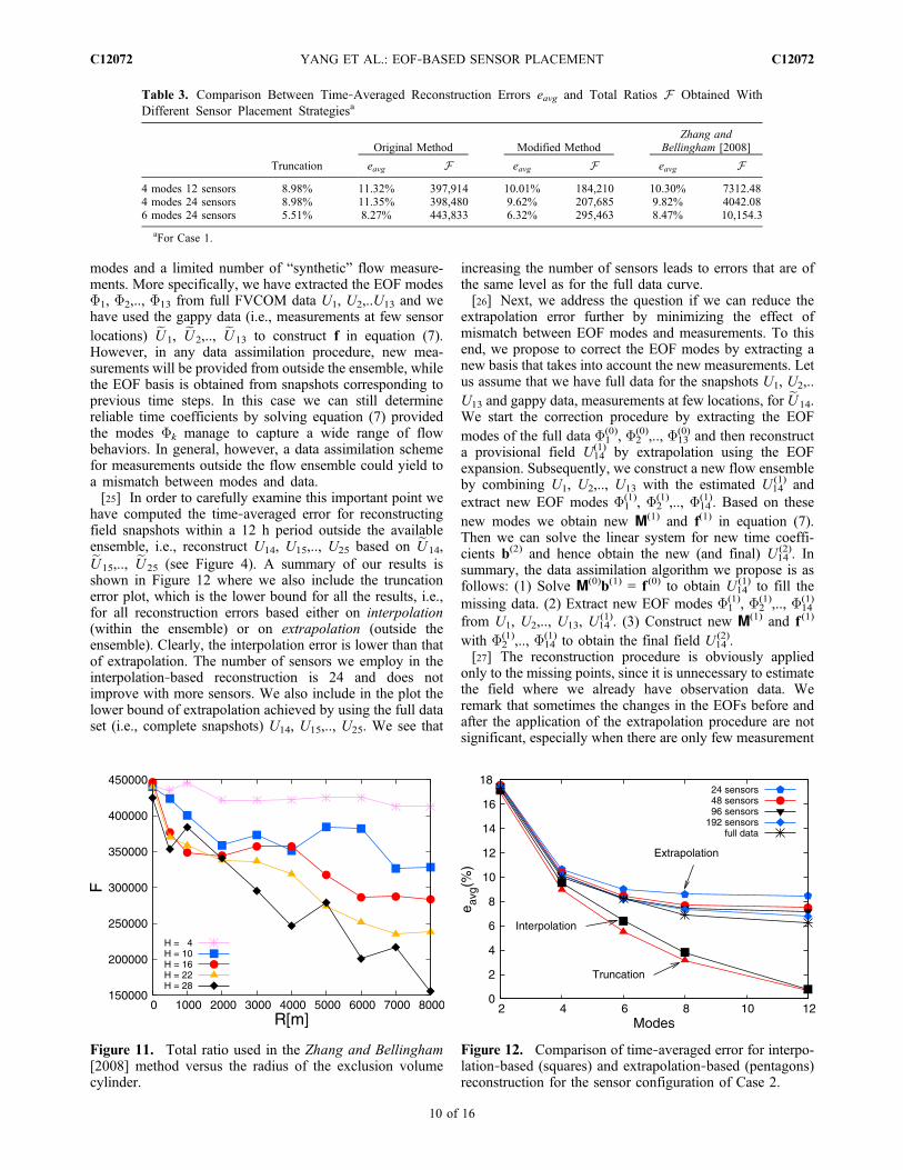
have computed the time‐averaged error for reconstructingfield snapshots within a 12 h period outside the availableensemble, i.e., reconstruct U14, U15,.., U25 based on eU14,eU15,.., eU25 (see Figure 4). A summary of our results isshown in Figure 12 where we also include the truncationerror plot, which is the lower bound for all the results, i.e.,for all reconstruction errors based either on interpolation(within the ensemble) or on extrapolation (outside theensemble). Clearly, the interpolation error is lower than thatof extrapolation. The number of sensors we employ in theinterpolation‐based reconstruction is 24 and does notimprove with more sensors. We also include in the plot thelower bound of extrapolation achieved by using the full dataset (i.e., complete snapshots) U14, U15,.., U25. We see that

increasing the number of sensors leads to errors that are ofthe same level as for the full data curve.[26] Next, we address the question if we can reduce the

extrapolation error further by minimizing the effect ofmismatch between EOF modes and measurements. To thisend, we propose to correct the EOF modes by extracting anew basis that takes into account the new measurements. Letus assume that we have full data for the snapshots U1, U2,..U13 and gappy data, measurements at few locations, for eU14.We start the correction procedure by extracting the EOFmodes of the full data F1

(0), F2(0),.., F13

(0) and then reconstructa provisional field U14

(1) by extrapolation using the EOFexpansion. Subsequently, we construct a new flow ensembleby combining U1, U2,.., U13 with the estimated U14

(1) andextract new EOF modes F1

(1), F2(1),.., F14

(1). Based on thesenew modes we obtain new M(1) and f(1) in equation (7).Then we can solve the linear system for new time coeffi-cients b(2) and hence obtain the new (and final) U14

(2). Insummary, the data assimilation algorithm we propose is asfollows: (1) Solve M(0)b(1) = f (0) to obtain U14

(1) to fill themissing data. (2) Extract new EOF modes F1

(1), F2(1),.., F14

(1)

from U1, U2,.., U13, U14(1). (3) Construct new M(1) and f (1)

with F2(1),.., F14

(1) to obtain the final field U14(2).

[27] The reconstruction procedure is obviously appliedonly to the missing points, since it is unnecessary to estimatethe field where we already have observation data. Weremark that sometimes the changes in the EOFs before andafter the application of the extrapolation procedure are notsignificant, especially when there are only few measurement

Figure 11. Total ratio used in the Zhang and Bellingham[2008] method versus the radius of the exclusion volumecylinder.

Figure 12. Comparison of time‐averaged error for interpo-lation‐based (squares) and extrapolation‐based (pentagons)reconstruction for the sensor configuration of Case 2.

Table 3. Comparison Between Time‐Averaged Reconstruction Errors eavg and Total Ratios F Obtained WithDifferent Sensor Placement Strategiesa

Truncation

Original Method Modified MethodZhang and

Bellingham [2008]

eavg F eavg F eavg F4 modes 12 sensors 8.98% 11.32% 397,914 10.01% 184,210 10.30% 7312.484 modes 24 sensors 8.98% 11.35% 398,480 9.62% 207,685 9.82% 4042.086 modes 24 sensors 5.51% 8.27% 443,833 6.32% 295,463 8.47% 10,154.3

aFor Case 1.


10 of 16

stations compared with the number of grid points on themodel grid.[28] Next we test this procedure by evaluating the error in

predicting the data for U14. Similar errors are obtained for allother snapshots. In Figure 13 we show results from thecorrection procedure for different number sensors when wesample the first 6 modes while in the reconstruction we useall modes. In other words, in step 1 we employ the first(most energetic) 6 modes, which are sampled uniformly(Case 2), while in step 3 we employ the new 13 modifiedEOF modes. In order to be able to study the error up to avery large number of sensors we perform this test withoutimposing the exclusion volume constraint, i.e., the cylindersize is set to zero. In particular, by doubling the number ofsensors each time we see initially a sharp decay of the error(up to 384 sensors), followed by a slower decay. As thenumber of sensors approaches the number of available datapoints from the FVCOM simulation the reconstruction errorapproaches zero.[29] We also see that the extrapolation error with 48

sensors is relatively large (about 11%) without the use of theconstraints in the sensor placement. Using the same numberof sensors (i.e., 48 sensors) and imposing the constraints weachieve a lower error of 4.36% using the above algorithmcompared with an error of 5.27% without reconstructing theEOF modes. In order to obtain this level of error with theoriginal method (no constraints) we see from Figure 13 thatwe would need more than 10,000 sensors! These resultsclearly point to the effectiveness of combining the twoaforementioned ideas, namely the use of constraints inplacing the sensors and the correction data assimilationprocedure presented in this section.

4. Uncertainty in Measurements

[30] So far we have used the FVCOM simulation outputsto generate “synthetic measurements” and have assumedthat there are no errors associated with such measurements.In this section, we will develop simple analytical expres-sions for the uncertainty of the reconstructed field assuming

that the sensor signals are affected by random noise whilethe EOF modes are deterministic, i.e., we consider the casewhere the right hand side in equation (7) contains uncer-tainty while the matrix M is constructed according to fulldeterministic EOF modes obtained from FVCOM simula-tion outputs. Specifically, we assume that the total velocitydetected by the sensors has the form

dðli; t; �Þ ¼ Uðli; tÞ þ �ðli; tÞ; ð14Þ

where {l1, .., lNs} are sensor locations, U is total velocity andx (li, t) (i = 1, .., Ns) are Ns zero‐mean uncorrelated Gaussianprocesses with standard deviation sx(li, t). In order toinclude the measurement uncertainty in the field recon-struction process we look for a representation of the totalvelocity in terms of random temporal modes and deter-ministic spatial modes [Mathelin and Le Maître, 2009;Venturi et al., 2008] as

Ueðx; t; xÞ ¼XKk¼1

�k t; xð ÞFk xð Þ; ð15Þ

where Fk are based on full FVCOM data. The notationUe(x, t; x) emphasizes that the stochastic total velocity (15)depends on the random vector

x ¼def �ðl1; t1Þ; ::; �ðlNs ; tSÞ½ �; ð16Þ

characterizing the measurement errors. Next we considerthe following functional:

J �k½ � ¼ZT

XNs

i¼1

d li; t; xð Þ �XKj¼1

�j t; xð ÞFj lið Þ" #2* +

dt; ð17Þ

where h·i denotes an average with respect to the joint prob-ability density of the random vector (16). More general dataassimilation schemes based on quadratic regularizationfunctionals can be considered. Minimization of (17) withrespect to hk yields the following Euler‐Lagrange equations:

XKk¼1

�k t; xð ÞXNs

i¼1

Fk lið ÞFm lið Þ ¼XNs

i¼1

d li; t; xmð ÞFm lið Þ: ð18Þ

This system can be rewritten in the same form as equation (7),i.e.,

XKj¼1

Fi;Fj

� �m�j ¼ d;Fið Þm; ð19Þ

provided the gappy inner product (5) is defined in terms of thesensor locations, that is m(x, t) = 1 if x = lj; zero otherwise. Ifthe matrix Mij = (Fi, Fj)m is not singular, then we obtain aunique solution to (19) in the form

�i t; xð Þ ¼XKj¼1

M�1ij d;Fj

� �m: ð20Þ

Now we can easily calculate the standard deviation of theestimate (15) based statistical assumption of the measure-ments errors. Specifically, by using the independence

Figure 13. Reconstruction error in snapshot 14th as a func-tion of the number of sensors deployed by using the EOF‐based extrapolation procedure. The sensor network is con-structed according to the original method, i.e., no constraintsare imposed (Case 2).


11 of 16

hypothesis of the measurement errors we obtain (repeatedindices are summed unless otherwise stated)

�Ueðx; tÞ ¼defffiffiffiffiffiffiffiffiffiffiffiffiffiffiffiffiffiffiffiffiffiffiffiffiffiffiffiffiffiffiffiffiffiffiffiffiffiffiffiffiffiffiffiffiffiffiffiffiffiffiffiffiffiffiffiffiffiffiffiðh�i�ki � h�iih�kiÞFi xð ÞFk xð Þ

p; ð21Þ

where

h�ii ¼ M�1ij hdðlj; t; xÞiFi lj

� �; ð22Þ

h�i�ki ¼ M�1im M�1

kn hdðlj; t; xÞdðlp; t; xÞiFmðljÞFnðlpÞ: ð23Þ

A substitution of (22) and (23) into (21) yields the followingformula

�Ueðx; tÞ ¼ �� lj; t� � ffiffiffiffiffiffiffiffiffiffiffiffiffiffiffiffiffiffiffiffiffiffiffiffiffiffiffiffiffiffiffiffiffiffiffiffiffiffiffiffiffiffiffiffiffiffiffiffiffiffiffiffiffiffiffiffiffiffiffiffiffiffiffi

M�1im M�1

kn FmðljÞFnðljÞFi xð ÞFk xð Þq

; ð24Þ

where sx (lj, t) denotes the standard deviation of the mea-surement errors at location lj.

Figure 14. Standard deviation of total velocity at the surface of the ocean for noisy sensors networks ofconfiguration Case 1. The measurement standard deviation is uniform and equal to sx ≡ 0.2. (a–c) Orig-inal sensor placement strategy. (d–f) Modified sensor placement strategy. It is seen that sensor networksobtained from the modified procedure with exclusion cylinder radius R = 3000 m significantly reduce thestandard deviation of the estimate Ue.


12 of 16

4.1. Results for Uniform Measurement Errors

[31] Let us assume that the standard deviation of themeasurement errors is a constant, i.e., sx(x, t) = sx. In thiscase equation (24) simplifies to

�UeðxÞ ¼ ��

ffiffiffiffiffiffiffiffiffiffiffiffiffiffiffiffiffiffiffiffiffiffiffiffiffiffiffiffiffiffiffiM�1

ik FiðxÞFkðxÞq

; ð25Þ

yielding to a time‐independent standard deviation of theestimate (15). This implies that even for a time‐dependentflow we have a simple time‐independent indicator field (25)that can be used to measure the quality of the sensor net-work. More specifically, formula (25) implies that thespectral radius of the matrix Mik

−1 affects the standard devi-ation of the estimate (15), in the sense that ifMik

−1 has a smallspectral radius then we can use a more noisy sensor network

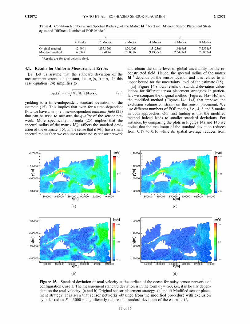
and obtain the same level of global uncertainty for the re-constructed field. Hence, the spectral radius of the matrixM−1 depends on the sensor location and it is related to anupper bound for the uncertainty level of the estimate (15).[32] Figure 14 shows results of standard deviation calcu-

lations for different sensor placement strategies. In particu-lar, we compare the original method (Figures 14a–14c) andthe modified method (Figures 14d–14f) that imposes theexclusion volume constraint on the sensor placement. Weuse different numbers of EOF modes, i.e., 4, 6 and 8 modesin both approaches. Our first finding is that the modifiedmethod indeed leads to smaller standard deviations. Forinstance, by comparing the plots in Figures 14a and 14b wenotice that the maximum of the standard deviation reducesfrom 0.19 to 0.16 while its spatial average reduces from

Table 4. Condition Number � and Spectral Radius r of the Matrix M−1 for Two Different Sensor Placement Strat-egies and Different Number of EOF Modesa

� r

4 Modes 6 Modes 8 Modes 4 Modes 6 Modes 8 Modes

Original method 12.9901 237.1705 1.2059e5 1.3123e4 1.6466e5 7.2554e7Modified method 6.6399 19.4194 27.0716 9.1836e3 2.3421e4 2.6852e4

aResults are for total velocity field.

Figure 15. Standard deviation of total velocity at the surface of the ocean for noisy sensor networks ofconfiguration Case 1. The measurement standard deviation is in the form sx = aU, i.e., it is locally depen-dent on the total velocity. (a and b) Original sensor placement strategy. (c and d) Modified sensor place-ment strategy. It is seen that sensor networks obtained from the modified procedure with exclusioncylinder radius R = 3000 m significantly reduce the standard deviation of the estimate Ue.


13 of 16

0.035 to 0.033. Our second finding shows that the conditionnumber and also the spectral radius of M−1 can be used toindicate small or large levels of uncertainty. Table 4 lists thecondition number and spectral radius of M−1 for the originaland the modified methods. In this case, a smaller conditionnumber or smaller spectral radius both lead to smallerstandard deviations. We have obtained similar results for thetemperature field (not shown here).

4.2. Results for Nonuniform Measurement Errors

[33] Next we study a more realistic case where the standarddeviation of x(x, t) is functionally dependent on the totalvelocity U(x, t). The simplest case is sx(x, t) = aU(x, t),where a is a positive constant (U ≥ 0 by construction, seeequation (8)). From equation (24) we easily obtain the fol-lowing analytical expression for the standard deviation of Ue

�Ueðx; tÞ ¼ �U lj; t� � ffiffiffiffiffiffiffiffiffiffiffiffiffiffiffiffiffiffiffiffiffiffiffiffiffiffiffiffiffiffiffiffiffiffiffiffiffiffiffiffiffiffiffiffiffiffiffiffiffiffiffiffiffiffiffiffiffiffiffiffiffiffiffi

M�1im M�1

kn FmðljÞFnðljÞFi xð ÞFk xð Þq

: ð26Þ

Comparing equation (25) with equation (26) we notice thatnow the standard deviation of the improved estimate dependson time. We can obtain numerical results by assigning atypical value a = 0.1 corresponding to 10% errors in mea-suring velocity. We can then compute the average andmaximum standard deviation of the estimate Ue. The resultsof these calculations are summarized in Figure 15. A com-parison between Figures 15a and 15b shows that the maxi-mum standard deviation reduces from 0.11 (original method)to 0.09 (modified method), while the average standarddeviation reduces from 0.0219 to 0.0202. Similar conclu-sions can be drawn by comparing Figures 15c and 15d. InFigure 16 we show the standard deviation obtained by usinga different number of sensors and 4 modes; here we considerall three cases reported in the first column of of Table 2.Table 5 reports on the condition number and on the spectralradius ofM−1 for variable sx = aU. We notice, that unlike theprevious case with constant sx, here smaller values ofspectral radius or condition number may be associated withlarger standard deviation, e.g., Case 3. This is expected,however, since the total velocity in this case directly appears

within the standard deviation equation (26) and therefore sUe

(x, t) is no longer a function of M−1 only.

4.3. Point Versus Line Measurements

[34] So far we have used measurements at specific pointsto reconstruct the velocity and temperature fields instead ofmeasurements in an entire vertical line that can be providedby oceanographic instruments, such as CDT. We haveconducted several tests using outputs of FVCOM for theNantucket Sound and we found that at least for the “mean”

Figure 16. Comparison between space‐time‐averagedstandard deviations for different sensor networks obtainedwith the modified method with 4 EOF modes.

Table 5. Condition Number � and Spectral Radius r of the MatrixM−1 for Different Sensor Networks Reported in Table 2a

4 Modes 6 Modes

� r � r

Case 1 7.08 5.33e3 13.35 8.79e3Case 2 4.38 4.06e3 8.46 5.65e3Case 3 3.22 3.64e3 7.46 5.63e3

aThe measurement standard deviations are in the form sx = aU.

Figure 17. Comparison between time‐averaged recon-struction error for the mean total velocity with “point mea-surements” and “line measurements,” where (a) 12 sensorsand 4 modes are used and (b) 24 sensors and 6 modes areused.


14 of 16

predictions the improvement with the line measurements isless than 1%. Typical results are shown in Figure 17 for4 and 6 modes reconstruction. However, line measure-ments help in reducing greatly the uncertainty as shown inthe corresponding plots in Figure 18. These results wereobtained using 4 modes for reconstruction and 12 sensorswhile the noise level was at 10% of the local velocity(nonuniform sx).

5. Summary

[35] Proper orthogonal decomposition can be used toanalyze the scale hierarchy of the ocean state dynamics butit can also provide good, if not optimum, locations forplacing sensors in adaptive sampling. This was demon-strated in previous work of Zhang and Bellingham [2008]and Yildirim et al. [2009], where different optimizationcriteria were employed. Specifically, the approach of Zhangand Bellingham employs a minimization principle based onthe normalized sum of the cross products of the EOF modeswhile the approach of Yildirim et al. identifies the sensorlocations simply as the extrema of the spatial EOF modes.

The simplicity of the latter technique, however, comes at aprice since the corresponding sensor network often suffersfrom redundant information due to the fact that multipleextrema may coexist in a local region, hence creating anoversampling in that region while neglecting equallyimportant dynamics elsewhere in the domain.[36] In order to make EOF‐based sensor placement

approaches more effective, we have modified the techniqueof Yildirim et al. [2009] by imposing a constraint thatexcludes other sensors to colocate in a cylindrical regionsurrounding a certain sensor. (Other types of exclusionvolumes such as spheres or cubes may be more appropriatefor sensor placement in simulations of ocean regions withmultiphysics dynamics. In this paper we have chosen thecylindrical exclusion volume because the Nantucket Soundexhibits a negligible vertical stratification due to its rathersmall depth.)[37] Our numerical tests suggest that there is an optimum

size of volume exclusion but we could not establish a rig-orous criterion to determine it a priori as it may be problemdependent. It may be possible that such an optimum size ofthe exclusion volume is related to an “effective wavelength”of the EOF modes but further work is required to documentthis hypothesis. In particular, due to the fact that the EOFmodes are multidimensional and cannot easily expressed intensor product form, especially for complex geometry domains,it is not clear how to determine such an effective wavelength.Nevertheless, we found that in all cases we tested any reason-able size of the cylindrical exclusion volume (e.g., a fewkilometers) leads to more accurate reconstruction than theoriginal method which does not employ any constraints. Forinstance, in one particular case we have studied for theNantucket Sound region, we have found that in order toreduce the reconstruction error to about 4% we would need48 sensors with the constrained sensor placement algorithmbut more than 10,000 sensors with the unconstrainedapproach of Yildirim et al. [2009].[38] Another modification, particularly important in data

assimilation, is the use of “imperfect” EOFmodes. In previouswork, we assumed that reconstruction of the field takes placewithin the time interval for which we have complete knowl-edge of the EOF modes. In practice, however, in assimilatingdata we have available EOF modes from previous time stepsand new measurements at later times, i.e., outside the intervalemployed for the computation of the EOF base. Hence, thereconstruction error is much larger due to extrapolation, and inour case it is almost doubled compared with the interpolationerror. To this end, we proposed a correction procedure thatreduces this error by recalculating the EOF modes andaccounting for the new information both on the right‐ and left‐hand side of equation (7). The computational complexity ofsolving this equation is very low as the rank of the matrixM isequal to the number of sensors, which is typically small.[39] Finally, we addressed the issue of uncertainty in the

measurements by adding Gaussian noise in the simulationoutputs of FVCOM. In particular, we considered two cases:first we assumed that the uncertainty in the measurements isconstant everywhere in the domain (i.e., sx is constant), andsecondly we allowed the uncertainty to vary in space andtime. In both cases, we derived analytically expressions forthe standard deviation of the reconstructed field in terms ofthe EOF modes and the matrix M. We demonstrated that the

Figure 18. Comparison between maximum (a) point‐wiseand (b) space‐time‐averaged standard deviation with “pointmeasurements” and “line measurements.”


15 of 16

levels of uncertainty in the reconstructed field are lowercompared to the reconstruction based on the original method.Lastly, we compared the effect of point measurements versusline measurements (e.g., in a water column using CDT) andwe found that there is no much difference in the mean of thereconstructed field but the standard deviation is reducedsubstantially by performing line measurements.[40] Taken together the above developments will improve

the effectiveness of EOF‐based sampling and reconstructionof the ocean state toward the ultimate goal of truly real‐timeadaptive sampling. However, further testing of this approachis required in regions with diverse dynamics in order todiagnose any limitations and possibly rectify them.

[41] Acknowledgments. We would like to thank the anonymousreferees for their insightful comments that helped us improve the qualityof our manuscript. This work was supported by ONR (N00014‐07‐1‐044), DOE (DE‐SC000254), and the MIT Sea Grant College program(NA‐060AR4170019).

ReferencesAlvera‐Azcárate, A., A. Barth, M. Rixen, and J. M. Beckers (2005), Recon-struction of incomplete oceanographic data sets using empirical orthogo-nal functions: Application to the Adriatic sea surface temperature, OceanModell., 9, 325–346.

Aubry, N., R. Guyonnet, and E. Stone (1991), Spatio‐temporal analysis ofcomplex signals: Theory and applications, J. Stat. Phys., 64, 683–739.

Beckers, J., and M. Rixen (2003), EOF calculations and data filling fromincomplete oceanographic datasets, J. Atmos. Oceanic Technol., 20(12),1839–1856.

Bekooz, G., P. Holmes, and J. Lumley (1993), The proper orthogonaldecomposition in the analysis of turbulent flows, Annu. Rev. Fluid Mech.,25, 539–575.

Cohen, K., S. Siegel, and T. McLaughlin (2003), Sensor placement basedon proper orthogonal decomposition modeling of a cylinder wake, paperpresented at 33rd Fluid Dynamics Conference and Exhibit, Am. Inst. ofAeronaut. and Astronaut., Orlando, Fla., 23–26 June.

D’Andrea, F., and R. Vautard (2001), Extratropical low‐frequency variabil-ity as a low dimensional problem. Part I: A simplified model, Q. J. R.Meteorol. Soc., 127, 1357–1375.

Dickey, T. (2003), Emerging ocean observations for interdisciplinary dataassimilation systems, J. Mar. Syst., 40–41, 5–48.

Everson, R., and L. Sirovich (1995), The Karhunen‐Loève procedure forgappy data, J. Opt. Soc. Am. A Opt. Image Sci., 12(8), 1657–1664.

Everson, R., P. Cornillon, L. Sirovich, and A. Webber (1995), An empiricaleigenfunction analysis of sea surface temperatures in the North Atlantic,J. Phys. Ocean., 27(3), 468–479.

Gunes, H., S. Sirisup, and G. E. Karniadakis (2006), Gappy data: To krig ornot to krig?, J. Comput. Phys., 212, 358–382.

Hendricks, J., R. Leben, G. Born, and C. Koblinsky (1996), Empiricalorthogonal function analysis of global TOPEX/POSEIDON altimeterdata and implications for detection of global sea rise, J. Geophys. Res.,101, 14,131–14,145.

Houseago‐Stokes, R. (2000), Using optimal interpolation and EOF analysison North Atlantic satellite data, Int. WOCE Newsl., 28, 26–28.

Lermusiaux, P., P. Malanotte‐Rizzoli, D. Stammer, J. Carton, J. Cummings,and A. Moore (2006), Progress and prospects of U.S. data assimilationin ocean research, Oceanography, 19, 172–183.

Mathelin, L., and O. Le Maître (2009), Robust control of uncertain cylinderwake flows based on robust reduced order models, Comput. Fluids, 38(6),1168–1182.

Mokhasi, P., and D. Rempfer (2004), Optimized sensor placement forurban flow measurement, Phys. Fluids, 16(5), 1758–1764.

Nguyen, N., A. Patera, and J. Peraire (2008), A ‘best points’ interpolationmethod for efficient basis approximation of parametrized functions, Int.J. Numer. Methods Eng., 73(4), 521–543.

Pedder, M., and D. Gomis (1998), Application of EOF analysis to the spatialestimation of circulation features in the ocean sampled by high‐resolutionCTD samplings, J. Atmos. Oceanic Technol., 15(4), 959–978.

Preisendorfer, W., and C. D. Mobley (1988), Principal Component Analy-sis in Meteorology and Oceanography, Elsevier, Amsterdam.

Rempfer, D. (2003), Low‐dimensional modeling and numerical simulationof transition in simple shear flow, Annu. Rev. Fluid Mech., 35, 229–265.

Sirovich, L. (1987a), Turbulence and the dynamics of coherent structures,part I: Coherent structures, Q. Appl. Math., 45, 561–571.

Sirovich, L. (1987b), Turbulence and the dynamics of coherent structures,parts II: Symmetries and transformations, Q. Appl. Math., 45, 573–582.

Sirovich, L. (1987c), Turbulence and the dynamics of coherent structures,part III: Dynamics and scaling, Q. Appl. Math., 45, 583–590.

Venturi, D. (2006), On proper orthogonal decomposition of randomly per-turbed fields with applications to flow past a cylinder and natural convec-tion over a horizontal plate, J. Fluid Mech., 559, 215–254.

Venturi, D., and G. E. Karniadakis (2004), Gappy data and reconstructionprocedures for flow past a cylinder, J. Fluid Mech., 519, 315–336.

Venturi, D., X. Wan, and G. E. Karniadakis (2008), Stochastic low‐dimensional modelling of a random laminar wake past a circular cylinder,J. Fluid Mech., 606, 339–367.

Wilkin, J. L., and W. G. Zhang (2006), Modes of mesoscale sea surfaceheight and temperature variability in the East Australian Current, J. Geo-phys. Res., 112, C01013, doi:10.1029/2006JC003590.

Willcox, K. (2005), Unsteady flow sensing and estimation via the gappyproper orthogonal decomposition, Comput. Fluids, 35(2), 208–226.

Yildirim, B., C. Chryssotomidis, and G. E. Karniadakis (2009), Efficientsensor placement for ocean measurement using low‐dimensional con-cepts, Ocean Modell., 27, 160–173.

Zhang, Y., and J. Bellingham (2008), An efficient method of selectingocean observing locations for capturing the leading modes and recon-structing the full field, J. Geophys. Res., 113, C04005, doi:10.1029/2007JC004327.

C. Chen, School for Marine Science and Technology, University ofMassachusetts Dartmouth, 706 S. Rodney French Blvd., New Bedford,MA 02744‐1221, USA.C. Chryssostomidis, Sea Grant College Program, Massachusetts Institute

of Technology, 77 Massachusetts Ave., E38‐300, Cambridge, MA 02139,USA.G. E. Karniadakis and X. Yang, Division of Applied Mathematics,

Brown University, 182 George St., Providence, RI 02912, USA. ([email protected])D. Venturi, Department of Energy, Nuclear and Environmental

Engineering, University of Bologna, Via Zamboni 33, Bologna I‐40126,Italy.


16 of 16

EOF based constrained sensor placement and field...

Documents

Transcript of EOF based constrained sensor placement and field...