Environmental Policy and Speculation on Markets for Emission Permits

Environmental Policy and Speculation on Markets forEmission Permits

By PAOLO COLLAw, MARC GERMAINz and VINCENT VAN STEENBERGHEww

wU niversita Bocconi zU niversites de Lille and U niversite catholiq ue de Louvain wwBelgianFederal Ministry for the Environment and U niversite catholiq ue de Louvain

Final version received 16 April 2010.

Speculators are active in large markets for emission permits such as those developing under the Kyoto

Protocol. Since speculators help risk-averse firms hedging the risk stemming from uncertain future

demand, their entry reduces permits’ expected returns and volatility. We characterize the optimal

environmental policy by the agency setting the total amount of permits when speculators are active.

Whenever the agency is sufficiently risk-tolerant, speculators improve aggregate welfare by fostering firms’

production. On the other hand, under a moderately risk-averse agency, the increase in production

volatility induced by speculators negatively affects social welfare.

INTRODUCTION

Tradable permits have recently gained much interest for the control of various airpollutants, such as sulphur dioxide, nitrogen oxides, volatile organic components andespecially greenhouse gases (GHGs) (see, for example, Stavins 2003). Markets for GHGemission permits have emerged following the signature of the Kyoto Protocol in 1997.The reason why carbon has a value is that governments have artificially created scarcityby capping the volume of emissions that industries and other sectors are allowed toproduce. The assetsFGHG reductionsFare created under government-establishedemissions trading systems (carbon allowances) or by individual projects that can claim‘carbon credits’ by demonstrating they are reducing GHGs. Given that countries’emissions constraints are binding from 2008 to 2012, the Protocol has already given riseto the largest markets for emission permits.

Beside the international market related to countries’ commitments under the KyotoProtocol, in 2005 the European Union (EU) launched an internal market for the trade ofGHG emission permits between private entities: the Emissions Trading Scheme (EUETS). Although EU ETS Phase I (2005–07) was to be considered as a pilot periodwithout strong emission reduction constraints, the EU ETS has quickly developed and isby now the largest market for emission permits, with a total value of nearly US$ 92 billionin 2008, which represents an 87% growth over 2007. For the sake of comparison, otherallowance-based initiatives (most notably, the Chicago Climate Exchange and the NewSouth Wales Market) accounted for roughly US$ 1 billion total value during the sameyear (see Capoor and Ambrosi 2009).

Activity on the carbon market has increased considerably since countries havehad to comply with their emission reduction obligations under the first commit-ment period of the Kyoto Protocol (2008–12). Moreover, because climate changeis a long-term challenge, very ambitious post-2012 strategies to curb GHG emissionswill need to be adopted (see Intergovernmental Panel on Climate Change 2007).A first step in this direction has been made by the EU, which has committed toemission reduction by 2020. In its so-called ‘climate and energy package’, the EU

© The Authors. Economica © 2010 The London School of Economics and Political Science. Published by Blackwell Publishing,

9600 Garsington Road, Oxford OX4 2DQ, UK and 350 Main St, Malden, MA 02148, USA

Economica (2012) 79, 152–182

doi:10.1111/j.1468-0335.2010.00866.x

envisages reaching these objectives with an extensive use of markets for emissionpermits by:

(1) extending the scope of the EU ETS;(2) linking the scheme to other existing or forthcoming national and regional initiatives

(e.g. the US Regional Greenhouse Gas Initiative (RGGI) in Northeastern and Mid-Atlantic states, or the various proposals for a cap-and-trade scheme in the USA,Australia, Canada, Japan and other countries);

(3) allowing for a significant use of Certified Emission Reductions (CERs).

In such a context, the future of markets for emission permits is promising.Emission permits share many characteristics with financial assets. The permits are

virtual assets: an agent holds a permit if this permit is registered on the account of thatagent by the environmental agency. Hence, on a given market, emission permits areperfect substitutes and their trade entails neither transportation nor inventory costs. Suchcharacteristics are favourable to the entry of investors whose trading activity is motivatedby speculative rather than compliance aims. Analyses of existing emission programmesreveal the presence of such agents on these markets. (See, for example, Schmalensee et al.(1998) for the US Acid Rain programme, and Fusaro (2005) for Southern California’sRECLAIM programme.) The appeal of CO2 emissions markets for investors is certifiedby the growing number of emissions indexes covering this segment. Back in 2006,Barclays Capital and UBS started tracking the most liquid emissions programmes withthe BCGI Global Carbon Index and UBS World Emissions Index, respectively. In April2008, Merrill Lynch and Societe Generale introduced their benchmarks, the MLCXGlobal CO2 Emissions Index and the SGI-Orbeo Carbon Credit Index. Most likely, thelack of correlation between tradable emissions products and the traditional asset classes(see Daskalakis et al. 2009) lies behind the attractiveness of carbon investing. Financialinstitutions and institutional investors are active on the international GHG marketsthrough so-called ‘carbon funds’, set up to finance CO2 emission reduction projects indeveloping countries and generate emission credits. Fusaro (2007) reports that over 60carbon funds were active during 2007, including three multi-billion funds (RNK Capital,Climate Change Capital and Natsource). Since its inception in 2005, several large banks(Barclays, Merrill Lynch, BNP, Fortis) have been heavily involved in market operationson the EU ETS, and in 2006 potential market speculators such as European and US‘green hedge funds’ have stepped in (see Convery and Redmond 2007). The beginning ofa global carbon market brings in all the risks of emerging markets, such as little pricediscovery, low liquidity and arbitrage opportunities. The main motive for speculators toapproach green markets is to profit from a mismatch in pricing, and strategies involvedirectional bets as well as cross-market arbitrage. For instance, there is some evidence(Fusaro 2007; Parsons et al. 2009) of speculation against the high spot prices in April2006, even if scarcity of permits supply in this early phase of the EU ETS did not allowmany players to short allowances. Buying low-priced credits and simultaneously sellingovervalued credits across markets has also proven to be a successful arbitrage strategy:for instance, CER purchase against European Allowance Unit sale allows for cashing inon the price differential (see Clemens Huettner’s commentary in July 2007 on the CER/EUA spread). Similarly, Fusaro (2005) notes the arbitrage opportunity offered under theUS Renewal Portfolio Standard (RPS) mechanism by short-selling energy credits in onestate and buying in another.

Nevertheless, to our knowledge, the literature on the tradable emission permitsinstrument has so far ignored these agents. Analysing speculation on markets for emission

Economica

© The Authors. Economica © 2010 The London School of Economics and Political Science

2012] ENVIRONMENTAL POLICY AND SPECULATION 153

permits would, however, be particularly relevant because speculators have an impact onthe equilibrium permit price and, consequently, on firms’ investment/production choices.Speculators stand ready to accommodate the excess demand of permits stemming fromfirms, and as such they serve as market-makers for pollution allowances. In a differentcontext, Bernardo and Welch (2004) consider the interaction between a pool of investorsfacing potential liquidity shocks and a sector of risk-averse speculators absorbingunwanted inventories. Among other things, Bernardo and Welch (2004) show that a stocktrades at a discount as a result of the inefficient allocation of risk that forces market-makers to hold positive inventories. Similarly to their work, we find that the permit’sequilibrium price includes a premium for holding inventories that firms are willing tounload. Such a change in the price signal in turn affects firms’ investment and productiondecisions. Therefore, when the environmental agency balances the environmental qualitywith the cost for the firms of reducing pollution, it should account for the impact ofspeculators. Investigating this last issue is precisely the aim of the present paper.

We develop a cap-and-trade model with three types of agents: firms, speculators andan environmental agency. While considering a single commitment period, the modeldescribes a multi-stage decision process. At the beginning of the commitment period, theagency optimally sets the aggregate amount of emission allowances and freely allocatesthem to polluting firms. During the commitment period, firms invest, produce andpollute, and trade permits between themselves and with (non-polluting) speculators onthe allowance market that opens at two trading rounds.

All agents are risk-averse and have to take some decisions under uncertainty. This isthe case for the environmental agency when it chooses the optimal quantity of permits,for the firms when they invest in capital, and for both firms and speculators when theyexchange permits during the first trading round. After uncertainty has been resolved,firms produce, pollute and trade permits during the second round, knowing that at theend of the commitment period they must surrender an amount of permits equivalent totheir emissions during the whole period.

The main results of our paper are as follows. The uncertainty faced by firms whenchoosing their level of capital makes them willing to sell (part of) their emission permitsduring the first trading round. Once uncertainty is resolved and capital has beenallocated, firms purchase back the permits at the second round. Speculators hold positiveinventories of permits between the two dates and earn positive expected returns ascompensation for their risk-bearing activity. While the environmental literature hasidentified different marginal costs of pollution control as the main source of producers’emission trading, we isolate risk-hedging as a second motive to trade permitsFsimilarlyto previous findings by Kawai (1983) for non-storable commodities. Regarding theenvironmental agency problem, our analysis reveals that social welfare depends on therisk-bearing capacity of the market (which in turn depends on the risk attitude of themarket participants, i.e. firms and speculators) as well as on the regulator’s attitudetowards risk. Whenever the agency is sufficiently risk-tolerant, speculators improveaggregate welfare by fostering firms’ production. On the other hand, in the presence of amoderately risk-averse agency, the increase in revenue volatility induced by speculatorsnegatively affects social welfare.

Our paper is closely related to previous contributions by Kawai (1983) and, morerecently, Baldursson and von der Fehr (2004). Kawai (1983) investigates the effects of afutures market on the price process of the underlying non-storable commodity. His setupinvolves futures trading between risk-averse agents (commodity producers and ‘pure’speculators) in the presence of a stochastic consumption demand. The futures market is

Economica


154 ECONOMICA [JANUARY

shown to transfer risk from producers (who supply the commodity under price uncertainty)to speculators, and the price for the insurance offered by speculators generates a positiverisk premium. The main difference between Kawai’s contribution and our paper is that weare concerned with the control of producers’ emissions, while he ignores the environment.As a consequence of our focus, we depart from Kawai in at least three aspects. First, weconsider storable pollution allowances instead of a non-storable commodity. Second, firmsin our model employ a two-input production function in lieu of a single-input one. Thisextension is important in our setting as a multiple-input function allows to consider bothoutput and substitution effects. FinallyFand more importantlyFwelfare depends not onlyon production (or consumption) but also on environmental damages. Thus theenvironmental agency must balance the social benefits of human activities with the socialcosts due to pollution when determining the optimal amount of permits.

Our approach is similar to the one used by Baldursson and von der Fehr (2004) inthat we consider risk-averse polluting firms deciding on the amount of capital (orabatement) under uncertainty. However, our paper differs from theirs in both itsmotivation and modelling framework. Baldursson and von der Fehr (2004) analyse theperformance of the tradable permits instrument with respect to the tax instrument.Among other things, they show that accounting for risk-aversion tends to increase therelative performance of taxes. They use a rather general formalization with respect to theobjectives of the firms, and consider uncertainty both at the aggregate (so-called‘extraneous’ risk) and firm-specific level. On the other hand, they do not consider theinterplay between producers and non-polluting agents, i.e. speculators, and do not modelthe behaviour of the environmental agency. Our aim is to analyse the impact ofspeculation on permits markets and, ultimately, on environmental policy. We make theadditional assumption of constant absolute risk-aversion in order to obtain closed-formsolutions and enrich the framework in three directions: we account for repeated permitstrading rounds, we introduce risk-averse speculators, and we compute the optimalamount of emission permits issued by the environmental agency.

The paper is organized as follows. In Section I we describe features of firms andspeculators, outline the sequence of decisions and analyse the permits marketequilibrium. Section II is devoted to the policy pursued by the environmental agencywhen setting the optimal amount of allowances to be issued. The impact of speculationand its interplay with optimal environmental policy is investigated in Section III, wherewe consider how speculators affect aggregate welfare as well as permits’ expected returnsand volatility. The robustness of our analysis to changes in the modelling framework isfurther discussed in Section IV, together with the policy implications. Finally, Section Vsummarizes our results and presents possible extensions to the current analysis.

I. THE MARKET FOR EMISSION PERMITS

Preliminaries: the agents

We consider three types of agents: firms, speculators and an environmental agency. Wefirst describe firms and speculators, assuming that there is a continuum of each of them,with nF (respectively nS) being the measure of firms (respectively speculators).

Firms Each firm, indexed by i, produces a homogeneous good via the same Cobb–Douglasconstant returns to scale production function kai e

1�ai , where ki and ei denote respectively the

level of capital and emissions used by firm i. Let y be the competitive price of the good to be

Economica



sold, so that the firm i value of output is

yi ¼ ykai e1�ai with 0<a<1:

The price y is random and encapsulates a price shock stemming from demanduncertainty and affecting all firms in the same way. Further, we assume that y is normallydistributed with mean m40 and variance s2.

When a firm emits pollutants, it must hold an amount of permits that is not lowerthan the level of emissions. Each firm freely receives from the environmental agency anamount of emission permits si0 and may sell some of its permits toFor purchase someadditional ones fromFother agents who are active in the permits market. For simplicity,we assume that the permits market opens at the beginning and at the end of thecommitment period. These two trading rounds are indexed by t (t ¼ 1,2), and the unitprice of permits on the market is then denoted by pt.

Firm i profit is

ð1Þ pFi ¼ pF ðki; si1; ei; yÞ ¼ ykai e1�ai � ciðkiÞ � p1ðsi1 � si0Þ � p2ðsi2 � si1Þ;

where ci(ki) is the cost of capital for firm i, and sit (t ¼ 1,2) is the amount of permits heldby firm i at the end of trading round t, i.e. firm i inventory of permits at stage t. Thereforeeach firm purchases (respectively sells) allowances at the trading round t if sit� sit � 140(respectively sit� sit � 1o0). We assume that the cost of capital satisfies ci(ki)40, c0i(ki)40and c00i(ki)X 0.

From equation (1), each firm’s total profit is composed of the revenues from thesales of the product yi, the cost of capital, and the cost (respectively benefits) of the netpermits purchases (respectively sales). As long as permit prices are strictly positive,the requirement that each firm must hold an amount of permits greater than or equal toits emissions level (si2X ei) will hold with equality, and we set si2 ¼ ei in equation (1).Equation (1) shows that a firm can reduce its emissions in two ways: either bysubstituting capital to emissions, or by decreasing its output. Investing in capitalusually takes more time than adjusting output. To account for that, we assume that ki ischosen under uncertainty at the beginning of the commitment period, and thatproduction yi and emissions ei result from ‘short-term decisions’ taken once uncertaintyis resolved.

Firms are risk-averse as captured by a constant absolute risk-aversion (CARA)function defined over their profits, and we let tFi

>0 denote the firm i absolute risk-tolerance coefficient (i.e. the inverse of the absolute risk-aversion parameter). The firms’aggregate risk-tolerance is then given by

ð2Þ tF �Z nF

0

tFidi:

Speculators Besides firms, speculators are active in the market for emission permits.Unlike firms, speculators do not produce or pollute and their profits result from theirtrading activity only. Speculators have no initial endowments of permits, i.e. all permitsissued by the agency are allocated to firms. Therefore speculator j profits from the pricedifference between the two trading rounds, by purchasing (or short-selling) permits in thefirst trading round and unwinding his position during the second trading round. Hencehis profit function is given by

ð3Þ pSj¼ pSðxj1; xj2; yÞ ¼ �p2xj2 � p1xj1;

Economica



where xjt is the purchase (xjt40) or sale (xjto0) of permits in trading round t, subject toxj1þ xj2X 0, i.e. speculators should hold non-negative inventories at the last stage. Aslong as permit prices are strictly positive, speculators will set xj2 ¼ � xj1.

We assume that speculators are also risk-averse with CARA utility function definedover final profits pSj

, and denote by tSj>0 the risk-tolerance coefficient of speculator j.

Finally, we let tS denote the speculators’ aggregate risk-tolerance, i.e.

ð4Þ tS �Z nS

0

tSjdj:

Environmental agency The agency is in charge of defining the total amount of emissionpermits

S0 ¼Z nF

0

si0di;

and of (freely) allocating allowances to firms. When setting S0, the environmental agencybalances the social gains from reducing the total amount of emissions with the losses inproduction due to the constraint on emissions. We assume that the agency maximizes the‘green’ revenue of the industry, i.e. the firms’ aggregate production (in value) less theirconsumption of capital and the damage costs due to pollutionZ nF

0

yidi �Z nF

0

ciðkiÞdi � dS0;

where dS0 is the total damage associated with pollution level S0. To be consistent withour formalization for the agents’ preferences in the economy, we also allow for constantabsolute risk-aversion on the part of the agency as captured by the risk-tolerancecoefficient tA40. The behaviour of the agency, leading to the definition of the optimalamount of permits by taking into account the damage costs due to emissions ofpollutants, is further analysed in Section II.

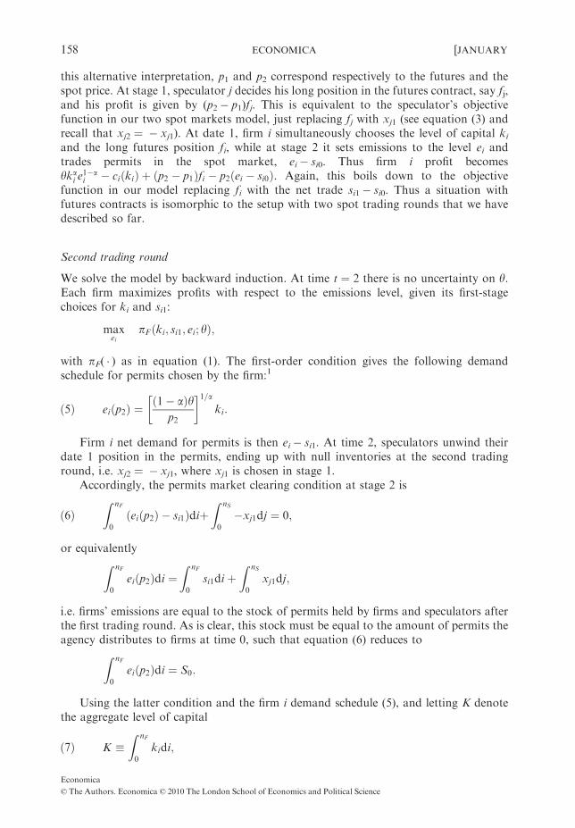
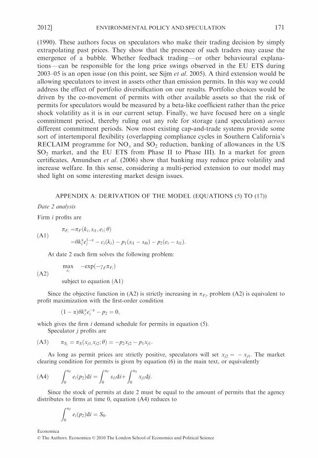
Timing The sequence of decisions is based on three stages, as follows. At stage 0, the agencyissues S0 permits and allocates them to firms. At stage 1, all agents face uncertainty on theprice shock y. Firms simultaneously choose the amount of capital ki and the emissionpermits inventory level si1. At the same time, speculators may also trade permits xj1. Then thevalue of y is revealed to all agents. At stage 2, firms decide on their output, or equivalently ontheir amount of emissions ei, and accordingly trade permits ei� si1. Speculators unwind theirtime 1 position, submitting � xj1. This sequence of decisions is illustrated in Figure 1.

Rather than a sequence of two spot markets, our model can equivalently be thoughtof as one where futures contracts are traded at date 1 for delivery at date 2. According to

Stage 0 Stage 1 Stage 2

Uncertaintyis revealed

Agency:S0

Firms: si1, kiSpeculators: xj1

Firms: eiSpeculators: xj2

FIGURE 1. Sequence of decisions.

Economica



this alternative interpretation, p1 and p2 correspond respectively to the futures and thespot price. At stage 1, speculator j decides his long position in the futures contract, say fj,and his profit is given by (p2� p1)fj. This is equivalent to the speculator’s objectivefunction in our two spot markets model, just replacing fj with xj1 (see equation (3) andrecall that xj2 ¼ � xj1). At date 1, firm i simultaneously chooses the level of capital kiand the long futures position fi, while at stage 2 it sets emissions to the level ei andtrades permits in the spot market, ei� si0. Thus firm i profit becomesykai e

1�ai � ciðkiÞ þ ðp2 � p1Þfi � p2ðei � si0Þ. Again, this boils down to the objective

function in our model replacing fi with the net trade si1� si0. Thus a situation withfutures contracts is isomorphic to the setup with two spot trading rounds that we havedescribed so far.

Second trading round

We solve the model by backward induction. At time t ¼ 2 there is no uncertainty on y.Each firm maximizes profits with respect to the emissions level, given its first-stagechoices for ki and si1:

maxei

pFðki; si1; ei; yÞ;

with pF( � ) as in equation (1). The first-order condition gives the following demandschedule for permits chosen by the firm:1

ð5Þ eiðp2Þ ¼ð1� aÞy

p2

� �1=aki:

Firm i net demand for permits is then ei� si1. At time 2, speculators unwind theirdate 1 position in the permits, ending up with null inventories at the second tradinground, i.e. xj2 ¼ � xj1, where xj1 is chosen in stage 1.

Accordingly, the permits market clearing condition at stage 2 is

ð6ÞZ nF

0

ðeiðp2Þ � si1ÞdiþZ nS

0

�xj1dj ¼ 0;

or equivalentlyZ nF

0

eiðp2Þdi ¼Z nF

0

si1di þZ nS

0

xj1dj;

i.e. firms’ emissions are equal to the stock of permits held by firms and speculators afterthe first trading round. As is clear, this stock must be equal to the amount of permits theagency distributes to firms at time 0, such that equation (6) reduces toZ nF

0

eiðp2Þdi ¼ S0:

Using the latter condition and the firm i demand schedule (5), and letting K denotethe aggregate level of capital

ð7Þ K �Z nF

0

kidi;

Economica



yields the second-stage permit price

ð8Þ p2 ¼ ð1� aÞ K

S0

� �a

y:

Note that p2 could in principle be negative, since the demand shock parameter isnormally distributed. However, as pointed out in Kawai (1983) and Vives (1984), one canmake the probability of negative prices (or output) arbitrarily small by choosing m and s2

such that the ratio m/s is large.2

Finally, in equilibrium, firm i emissions are given by

ð9Þ ei ¼S0

Kki:

First trading round

Firms At time t ¼ 1, all agents face uncertainty about the date 2 product demand. Eachfirm solves maxki ;si1EðuFi

ðpFiÞÞ subject to the permit price and emissions level prevailing

at date 2, where uFi( � ) denotes the firm i utility function. For reasons of tractability, we

focus on the particular case where ci(ki) ¼ rki with r40. This corresponds to a linearcapital cost function that is identical across firms. Therefore firms differ only in their risk-tolerance coefficient tFi

and in their initial endowment of allowances si0. (In Section IVwe discuss the case of heterogeneous capital cost functions.) Substituting the equilibriumvalues for p2 and ei (see equations (8) and (9)) into the expression for pFi

as given inequation (1) yields

ð10ÞpFi¼pF ðki; si1; yÞ

¼ yKa

Sa0

aS0

Kki þ ð1� aÞsi1

� �� rki � p1ðsi1 � si0Þ:

Since the price shock is assumed to be normally distributed with mean m and variances2, profits in equation (10) are also normally distributed. As is known (see, for example,Lintner 1969), optimization of a CARA utility function defined over a normal randomvariable allows us to write the firm i maximization problem as

ð11Þ maxki ;si1

EðuFiðpFiÞÞ ¼ max

ki ;si1mF ðki; si1Þ � ð2tFi

Þ�1s2Fðki; si1Þ;

where mF( � ) and s2Fð�Þ denote respectively the mean and the variance of firm i profits.Optimality conditions for problem (11) allow us to write aggregate capital in

equation (7) as

ð12Þ Kðp1Þ ¼ap1S0

ð1� aÞr ;

while for aggregate permit inventories

S1 �Z nF

0

si1di;

we have

ð13Þ S1ðp1Þ ¼tF

ð1� aÞ2ð1�aÞs2r

a

� �2a 1

pa1ð1� aÞ1�a a

r

� �am� p1�a1

h i� aS0

1� a;

Economica



where tF is given in equation (2). The demand schedule in equation (13) shows that theamount of permits held by firms at stage 1 is decreasing in the amount of permits issued(S0) as well as the permit price (p1), increasing in the expected price shock (m), anddecreasing in its uncertainty (s2).

Speculators The speculators’ problem is defined along the same lines as for firms. Eachspeculator solves maxxj1 EðuSj

ðpSjÞÞ, where uSj

( � ) denotes the speculator j utility function.Given the equilibrium price p2 (see equation (8)), profits pSj

as defined in equation (3) arenormal with first two moments mS( � ) and s2Sð�Þ. Hence the maximization problembecomes

maxxj1

EðuSjðpSjÞÞ ¼ max

xj1mSðxj1Þ � ð2tSj

Þ�1s2Sðxj1Þ;

and the optimal demand (or inventory) of speculator j is

ð14Þ xj1ðp1Þ ¼tSj


a

� �2a 1


r

� �am� p1�a1

h i:

The speculator j demand schedule in equation (14) is negatively sloped, i.e. xj1depends negatively on p1. Moreover, the dependence on m and s2 is analogous to thatfound for firms (see equation (13)).

Finally, we let X 1 denote the aggregate speculators’ demand, i.e.

X 1 �Z nS

0

xj1dj:

Equation (14) then yields

ð15Þ X 1ðp1Þ ¼tS


a

� �2a 1


r

� �am� p1�a1

h i;

where tS is given in equation (4).

Market eq uilibrium The first-stage market clearing condition isZ nF

0

ðs1ðp1Þ � si0ÞdiþZ nS

0

xj1ðp1Þdj ¼ 0;

which can be equivalently rewritten in aggregate terms as

S1ðp1Þ þ X 1ðp1Þ ¼ S0:

Let t denote the risk-bearing (or risk-tolerance) capacity of the market, i.e.

ð16Þ t � tF þ tS;

where tF and tS are defined in equations (2) and (4). As is clear, the market risk-bearingcapacity is an increasing function of all agents’ degree of risk-tolerance, tFi

and tSj, as

well as their measure, nF and nS.Using the permit demand schedules in equations (13) and (15) together with the

market risk-bearing capacity (see equation (16)), the first-stage permit price solves the

Economica



implicit function

ð17Þ S0 ¼ts2ð1� aÞrap1

� �am� r

a

� �a p1

1� a

� �1�a� �:

Equation (17) does not lend itself to explicitly compute3 the equilibrium price p1.However, the existence and uniqueness of such an equilibrium price on the positive half-line are addressed in the following proposition:

Proposition 1. For any finite positive S0, there exists a unique equilibrium price p1[<þþ.

We now investigate some comparative statics of the equilibrium price p1.

Corollary 1. For any finite positive S0, the equilibrium price p1 increases with t.

The increase in the market risk-bearing tolerance reduces the negative effect that theuncertainty about production conditions, i.e. date 2 price movements, exerts on marketparticipants’ expected utility. Therefore at date 1, firms are more willing to hold on totheir permits and/or speculators are more prone to buy permits. Lower supply and higherdemand would move p1 up. As clearly emerges from inspection of equation (12), whenpermits become more expensive, firms substitute allowances with capital, so that Kincreases together with aggregate production (in value)

ð18Þ Y �Z nF

0

yidi ¼ yKaS1�a0 :

This clarifies the role played by speculators in helping firms hedging their productionrisk.

Corollary 2 . For any given t, the equilibrium price p1 decreases with S0.

According to Corollary 2, the date 1 permit price decreases when the totalsupply of permits increases. This is rather intuitive and stems from the fact that demandcurves for permits are downward sloped, as previously noted (see equations (13) and(15)).

We now turn to investigate the relationship between permit prices. Takingexpectations on both sides of equation (8) yields

ð19Þ Eðp2Þ ¼ ð1� aÞ K

S0

� �a

m;

while equation (12) can be equivalently rewritten as

ð20Þ pa1 ¼ð1� aÞr

a

� �aK

S0

� �a

:

Then combining equations (19) and (20) leads to

Eðp2Þpa1¼ ð1� aÞ1�a a

r

� �am;

which says that the expected date 2 allowance price is an increasing and concave functionof p1. Let R ¼ (p2/p1)� 1 denote the (net) return earned on permits between the two

Economica



trading rounds, so that expected returns are given by E(R). We establish some propertiesof the unique equilibrium in the permits market by means of the following proposition:

Proposition 2 . In equilibrium:

1. permits’ expected returns are strictly positive, i.e. E(R)40;2. speculators buy permits at the first trading round, i.e. X 140.

Proposition 2 generalizes previous results from Kawai (1983) to the case of our two-input production function. Positive expected returns obtain as the compensation paid byfirms to speculators for holding risky permit inventories. Besides the main source ofemission trading, i.e. differences across firms in their marginal cost of pollution control,Proposition 2 identifies risk-hedging due to uncertain demand conditions in the productmarket as a second motive to trade permits. More precisely, if we additionally considerfully identical firms (i.e. with respect to the cost function and the risk-tolerance), permitstrading will take place between firms and speculators.

II. OPTIMAL ENVIRONMENTAL POLICY

The role of the regulator within a cap-and-trade system is to determine the amount ofpermits S0, i.e. the level of pollution. (See Convery et al. (2008) for the role played by theEuropean Commission in reviewing National Allocation Plans and setting the aggregatecap.) As explained in the first subsection of Section I, the agency maximizes the firms’aggregate production (in value) less their consumption of capital and the damage costsdue to pollution. This welfare criterion (‘green’ revenue) has been used within partialequilibrium models similar to ours (see, for example, Barrett 1994; Ulph 1996; Germainet al. 2004a,b).

Since K ¼R nF0 kidi (see equation (7)) and in equilibrium S0 ¼

R nF0 eidi, the agency

objective is defined in terms of the aggregate welfare

ð21Þ Y � rK � dS0;

where Y denotes the aggregate production defined in equation (18). Letting mA( � ) ands2Að�Þ denote the first two moments of the aggregate welfare, i.e.

ð22Þ mAðS0Þ ¼ Eð Y Þ � rK � dS0;

ð23Þ s2AðS0Þ ¼ V ðY Þ;

the agency problem can be written as

ð24ÞmaxS0

WðS0Þ ¼ maxS0

mAðS0Þ � ð2tAÞ�1s2AðS0Þ

subject to equations ð12Þ; ð17Þ; ð22Þ; ð23Þ andS0*0:

Let S0 be a solution to the optimization problem (24), and let WðS0Þ be thecorresponding welfare, i.e. WðS0Þ ¼ mAðS0Þ � ð2tAÞ�1s2AðS0Þ. The remainder of theanalysis concerns the characterization of a non-negative solution to (24), as well asthe comparative statics of the aggregate welfare with respect to the marginal damage d.The existence and uniqueness of a solution to problem (24) are addressed in the followingproposition:

Economica



Proposition 3 . The agency optimization problem admits a unique positive maximumS0>0 for which WðS0Þ>0 if and only if

ð25Þ d< d � ð1� aÞ ar

� �am

h i1=ð1�aÞ:

In words, a necessary and sufficient condition for the socially optimal pollution level tobe positive is that the marginal willingness to pay for the environment is not too large.Indeed, if marginal damage costs are large, i.e. d*d, the agency chooses to issue and allocateno emission permits at all, so that productionFand therefore pollutionFwill not take place.The role played by the marginal damage is further characterized in the following proposition:

Proposition 4. If d< d, then both the optimal amount of permits S0, and the associatedsocial welfare WðS0Þ, decrease with d.

Proposition 4 asserts thatFconsistently with the intuition behind Proposition 3Fthehigher the marginal damage (d), the lower the amount of permits issued and the lower thesocial welfare.

III. THE IMPACT OF SPECULATION

We now turn to evaluate how speculators affect the equilibrium described in Sections Iand II, focusing on the optimal amount of allowances issued by the agency (and theassociated aggregate welfare) as well as on expected permits return and volatility.

Welfare analysis

It turns out that what matters for the socially optimal level of pollutionFas well as theassociated welfareFis the relationship between the agency and the market risk-bearingcapacity, i.e. between tA and t:

Proposition 5. Let d<bd. ThendS0

dt*0 and

dWðS0Þdt

*0 if tA*t;

dS0

dt<0 and

dWðS0Þdt

<0 if tA<t:

According to Proposition 5, pollution and social welfare exhibit a non-monotonicrelationship with the risk-bearing capacity of the market. In fact, both S0 andWðS0Þ increasein the market risk-tolerance when t lies between tF and tA, reach a maximum at t ¼ tA, anddecrease4 for t4tA. The intuition underlying such behaviour goes as follows. Note fromequations (22), (23) and (24) that the agency objective function can be rewritten equivalently as

ð26Þ WðS0Þ ¼ PAðS0Þ � dS0;

with

ð27Þ PAðS0Þ ¼ ½Eð Y Þ � rK� � ð2tAÞ�1 V ð Y Þ;

where both K and Y are functions of S0 (see equations (12) and (18)). Expression (26)clarifies that there are two factors affecting aggregate welfare. The first is the social utility of

Economica



production PAðS0Þ, which itself comprises two terms by equation (27): the expectedaggregate production (in value) net of firms’ consumption of capital, E(Y )� rK, andaggregate production variability as perceived by the (risk-averse) environmental agency,ð2tAÞ�1 V ð Y Þ. Thus PAðS0Þ is the risk-adjusted social utility of production. Firms’ activityalso brings social disutility (pollution), which accrues to the second term in equation (26),dS0. If marginal damage costs are not too large (see Proposition 3), then the agency sets theinitial amount of permits to the social optimum S0 equating marginal utility of production tomarginal disutility of pollution, i.e.

ð28Þ @

@S0PAðS0Þ ¼ d:

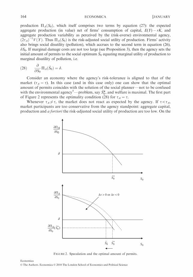
Consider an economy where the agency’s risk-tolerance is aligned to that of themarket (tA ¼ t). In this case (and in this case only) one can show that the optimalamount of permits coincides with the solution of the social plannerFnot to be confusedwith the environmental agency5Fproblem, say Sn

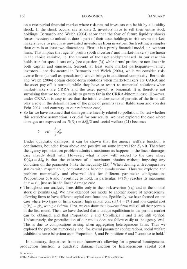
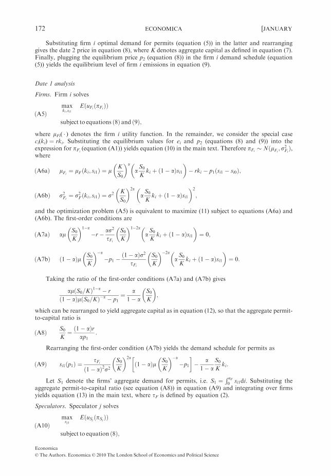
0 , and welfare is maximal. The first partof Figure 2 represents the optimality condition (28) for tA ¼ t.

Whenever tA 6¼ t, the market does not react as expected by the agency. If totA,market participants are too conservative from the agency standpoint: aggregate capital,production and a fortiori the risk-adjusted social utility of production are too low. On the

0A

S∂Π∂

δ

0S*0S

0

AS

∂Π∂

δ

0S*0S0S ′

Δ� > 0 or Δ� < 0

*0

0

ˆ( )A SS

∂Π∂

FIGURE 2. Speculation and the optimal amount of permits.

Economica



contrary, when t4tA, the agency is more risk-averse than the market. In such a casemarket participants are ‘too liberal’ from the agency’s point of view: both K and Y aretoo large, and output volatility V ( Y ) negatively affects the social utility of productionby (27).

Moreover, the change in the market risk-tolerance affects the marginal utility ofproduction @PA=@S0 as well. Starting from the situation tA ¼ t, either a decrease (Dto0)or an increase (Dt40) in the market risk-tolerance implies that the market no longer reactsas expected by the agency, so that @PAðS0Þ=@S0 moves inwards as depicted in the secondpart of Figure 2. The agency cannot keep the same amount of permits because at Sn

0 theequality between social marginal benefits and costs in equation (28) is violated, i.e.@PAðSn

0Þ=@S0<d. The agency reacts to the change in the market risk-aversion by reducingthe number of permits to S 00< Sn

0 . Note that this reduction further decreases the risk-adjusted social utility of production as measured by the area under the solid curve @PA=@S0

over the interval ½S 00; Sn0 �. However, this negative effect on social welfare is more than

compensated by the simultaneous reduction in pollution as measured by the rectangle ofwidth d and length Sn

0 � S 00. Therefore the marginal social utility of production increasesfrom @PAðSn

0Þ=@S0<d to @PAðS 00Þ=@S0 ¼ d, and optimality is restored.

Speculation and policy implications The policy implications of our analysis with respectto speculation are therefore as follows. Suppose that only firms are allowed to trade inthe permits market, i.e. nS ¼ 0, so that the market risk-bearing capacity coincides with tF.Provided that marginal damage costs are sufficiently low, the agency optimally sets thenumber of permits to S0, thus achieving the aggregate welfare WðS0Þ (see Proposition 3).How does the agency react if the market opens to speculators as well? As is clear fromequation (16), the entry of speculators increases the market risk-bearing capacity, t4tF.If tA4tF, then the regulator should allow speculators on the permit market under thecondition that they do not increase the market risk-bearing capacity t too much (that is,above tA). If tAotF, then firms alone already make decisions that are too ‘risky’ from theagency’s perspective, and speculators’ entry should be avoided.

Permits market analysis

Eq uilibrium price of permits It is of particular interest to understand how speculatorsaffect the equilibrium price p1. From equation (17) it follows that

ð29Þ dp1

dt¼ @p1@tþ @p1@S0

dS0

dt:

Equation (29) shows that the impact of speculation on p1 can be disentangled intotwo components. First, a direct effect (measured by @p1=@t) that is for a given amount ofinitial permits S0. Speculators’ demand for emission allowances has an impact on theequilibrium price p1. Changes in permit prices affect the optimal allocation of firms’resources between capital and energy, and changes in firms’ production plans will in turnhave an effect on the aggregate welfare. The direct effect therefore brings in a secondcomponent measured by the second term on the right-hand side of equation (29). Thissecond effect takes into account the reaction of the agency to the entry (or exit) ofspeculators that modifies t. Such reaction translates into a variation of the optimalamount of permits (measured by dS0=dt), which in turn induces a further change in p1(measured by @p1=@S0). To summarize, speculation exerts a direct effect on the permits

Economica



equilibrium price when speculators submit their demand, and an indirect effect throughthe amount of permits optimally chosen by the agency.

The overall effect on p1 is non-trivial. Indeed, from Corollary 1 we have that@p1=@t>0 since speculators help firms hedging their production risk. Second, demandschedules for permits are downward sloping and Corollary 2 yields @p1=@S0<0 . Third,the impact of a change in t on S0 is more articulated, as Proposition 5 reveals.Nevertheless, we are able to prove the following proposition:

Proposition 6 . The equilibrium price p1 ¼ p1ðS0Þ increases with t.

We know from Proposition 5 that when the market risk-bearing capacity issufficiently large, i.e. t4tA, the agency reduces the amount of permits to slow downeconomic activity. In this case p1 unambiguously increases due to the combined effect ofimproved hedging motives and reduced permit supply. However, when the agency ismore risk-tolerant with respect to the market, i.e. tAX t, the direct and indirect effect ofspeculation act in opposite directions. On the one hand, speculators help firms hedgingtheir risk, and permits trade at a higher price (see Corollary 1). On the other hand, theagency issues more permits in order to foster production, thus lowering the equilibriumpermit price at date 1. The overall effect on p1 is therefore a priori ambiguous once theagency’s reaction is taken into account.

According to Proposition 6, the direct effect dominates the indirect one, i.e. the priceincrease due to the improved risk-hedging motives following the speculators’ entry alwaysoffsets the price decrease triggered by changes in the optimal amount of permits when tAX t.

Expected returns and volatility We now focus on studying the impact of speculation onexpected returns E(R), and their volatility V (R) ¼ var(R). From a policy orientedperspective, it is of major importance to identify the impact of the underlying parameterson expected returns, since they measure the speculators’ profit opportunitiesFand thusaffect their incentives to enter the emission permits market. The attention devoted to theimpact of speculation on price fluctuations in financial markets by a wide range of agents,including authorities monitoring markets’ behaviourFsee, for example, the report onhedge funds and their impact on market volatility by the UK Financial ServicesAuthority (2005)Fmotivates the analysis of return volatility as well.

In order to understand the impact of speculation on expected returns and volatility,note that substituting aggregate capital (see equation (12)) into the date 2 price (seeequation (8)) yields

ð30Þ 1þ R ¼ ar

� �a 1� ap1

� �1�ay;

which says that the return on allowances is inversely related to the first trading roundprice. Using equation (30), expected returns and volatility are

ð31Þ EðRÞ ¼ ar

� �a 1� ap1

� �1�am� 1;

ð32Þ V ðRÞ ¼ ar

� �2a 1� ap1

� �2ð1�aÞs2:

Economica



Since E(R) and V (R) are inverse functions of p1 according to equations (31) and (32),changes in the market risk-bearing capacity that affect the date 1 equilibrium price in onedirection will exert the opposite effect on expected returns and volatility.

Thanks to Proposition 6 and equations (31) and (32), we can now understand theeffect of speculation on expected returns and volatility:

Proposition 7 . Both expected returns and volatility decrease with t.

When the market risk-bearing capacity increases, holding permit inventories becomesless risky and the compensation for holding them, i.e. E(R), necessarily decreases.Moreover, as the market risk-aversion lowers, we have from Proposition 6 that p1increases. Therefore the combined effect of higher date 1 prices and lower expectedreturns is a decrease in permits volatility V (R).

IV. DISCUSSION

Results robustness

The sharp policy implications delivered by our model mainly hinge on the comparativestatics that we perform on several variables of interest. We now describe how ourpredictions are robust to changes in the assumptions used so far. These changes relate tothe CARA utility function, the Cobb–Douglas production function, the linearity of thedamages and firms’ cost heterogeneity.

� We have checked that the existence of an equilibrium price in the permits market (seeProposition 1) extends to general linear homogeneous production functions

yi ¼ ykifei

ki

� �;

where f( � ) satisfies standard conditions. We can indeed derive restrictions on thebehaviour of f when the energy-to-capital ratio diverges to þ 1 so that the existenceand uniqueness of a positive equilibrium permit price are guaranteed.6 Under suchrestrictions on the production function, Proposition 2 and Corollaries 1 and 2 still holdtrue. As for the agency problem, we were able to derive an upper bound on themarginal damage d such that the agency welfare maximization admits a positivemaximum, thus generalizing the inequality (25) in Proposition 3. Unfortunately,establishing uniqueness of the maximum in this general case appears to be much moredifficult. However, we managed to show analytically that the social welfare functionadmits a local maximum at t ¼ tA and that Propositions 6 and 7 go through locallyaround that point.

� In order to assess the relevance of the CARA utility function for our results, we haveexplored the constant relative risk-aversion (CRRA) case. To our knowledge, noclosed-form solutions for asset demand are available even in simpler static portfolioproblems with CRRA and normally distributed pay-offs. Thus we have explored thecase of a binomial random shock.7 Already at the level of the market equilibrium (i.e.for S0 given) computations turn quickly to a highly non-linear system of equations thatcan be solved only numerically, and multiple equilibrium values of the permit priceare possible. This loss in tractability has to be expected since it arises even in

Economica



on a two-period financial market where risk-neutral investors can be hit by a liquidityshock. If the shock occurs, say at date 2, investors have to sell their entire stockholdings. Bernardo and Welch (2004) show that the fear of future liquidity shocksforces investors to unload at date 1 part of their asset holdings to risk-averse market-makers ready to purchase unwanted inventories from investors. Such setting is simplerthan ours in at least two dimensions. First, it is a purely financial model, i.e. withoutfirms. This implies that agents’ profits (both investors’ and market-makers’) are linearin the choice variable, i.e. the amount of the asset sold/purchased. In our case thisholds true for speculators only (see equation (3)) while firms’ profits are non-linear inboth capital and emissions. Second, at least some market participantsFnamelyinvestorsFare risk-neutral in Bernardo and Welch (2004), while we consider risk-averse firms (as well as speculators), which brings in additional complexity. Bernardoand Welch (2004) obtain closed-form solutions when market-makers are CARA andthe asset pay-off is normal, while they have to resort to numerical solutions whenmarket-makers are CRRA and the asset pay-off is binomial. It is therefore notsurprising that we too are unable to go very far in the CRRA-binomial case. However,under CRRA it is easy to see that the initial endowments of permits of the firms willplay a role in the determination of the price of permits (as in Baldursson and von derFehr 2004, and contrary to our reference case).

� So far we have assumed that damages are linearly related to pollution. To test whetherthis restrictive assumption is crucial for our results, we have explored the case wheredamages are expressed as DðS0Þ ¼ dS2

0=2 and social welfare (21) becomes

Y � rK � d2S20:

Under quadratic damages, it can be shown that the agency welfare function iscontinuous, bounded from above and positive on some interval for S040. Thereforethe agency optimization problem admits a maximum as happens in the linear damagescase already dealt with. However, what is new with respect to the case whereD(S0) ¼ dS0 is that the existence of a maximum obtains without imposing anycondition on the parameter d like the inequality (25).8 When dealing with comparativestatics with respect to t, computations become cumbersome. Thus we explored theproblem numerically and observed that for different parameter configurationsPropositions 5, 6 and 7 continue to hold. In particular, WðS0Þ reaches its maximumat t ¼ tA, just as in the linear damage case.

� Throughout our analysis, firms differ only in their risk-aversion (tFi) and in their initial

stock of permits (si0). We have extended our model to another source of heterogeneity,allowing firms to have different capital cost functions. Specifically, we have focused on thecase where two types of firms coexist: high capital cost (cðkiÞ ¼ rki) and low capital cost(cðkiÞ ¼ rki, with r< r) firms. First, we can show that low-cost firms will sell all their permitsin the first round. Then, we have checked that a unique equilibrium in the permits marketcan be obtained, and that Proposition 2 and Corollaries 1 and 2 are still verified.Unfortunately, the generalization of our results does not follow easily at the agency level.This is due to complications arising when aggregating heterogeneous firms. Thus weexplored the problem numerically and, for several parameter configurations, social welfareexhibits the same behaviour as in Proposition 5, and Propositions 6 and 7 continue to hold.9

In summary, departures from our framework allowing for a general homogeneousproduction function, a quadratic damage function or heterogeneous capital cost

Economica



functions are likely not to impair our analysis. Indeed, all our results at the permitsmarket level (in particular, Proposition 2) generalize to these alternative settings.Moreover, even if we cannot replicate analytically all our results at the agency level, ourexploratory analyses strongly suggest that they are very likely to be robust to thedepartures hereby considered. In particular, social welfare shows the same pattern as inProposition 5. However, since computations immediately become too cumbersome, wewere not able to investigate further if our results are robust when dropping the CARA infavour of the CRRA utility function.

Policy implications

Three important issues deserve additional comments. The first two relate to our mainresults, namely the comparative statics for permit prices, expected returns and volatility(Propositions 6 and 7) and social welfare (Proposition 5). The third issue concerns short-selling constraints and the introduction of derivatives.

1. A careful look at existing markets such as the US market for SO2 permits or theEuropean market for CO2 permits reveals that permit prices may significantlyfluctuate over time. Of course, numerous elements explain these fluctuations, such aschanges in oil or electricity prices, weather, political decisions, etc.10 Our findingssuggest that, besides these exogenous shocks, risk-aversion and risk-hedgingbehaviour may explain part of the price movements observed on markets foremission permits.11 Indeed, we have shown that (expected) permit prices tend to risethrough time (see Proposition 2). This result departs from the existing contributionson transaction costs (see, for example, Stavins 1995) or intermediation (see, forexample, Germain et al. 2004a) in markets for emission permits, which emphasize thepossible existence of a spread (i.e. a difference between the price at which permits aresold and the price at which permits are purchased). Here, we observe an intertemporalspread, i.e. a situation in which expected permit prices change through time.Moreover, we have also shown that the volatility of the prices is influenced by thepresence of speculators and, more generally, by the market risk-tolerance. An increasein the risk-bearing capacity tends to stabilize prices, and vice versa.

2. Classical analyses of the tradable emission permits instrument do not account for theparticipation of speculators on the market. The main policy implications of ouranalysis depend on the degree of risk-aversion of the agency with respect to that offirms and speculators. Since the entry of speculators into the permits market increasesthe overall risk-bearing capacity, by Proposition 5 institutional rules should favourthe presence of speculators on markets for emission permits (by contrast with thesituation where only polluting firms are present on the market). However, allowingspeculators to operate on the emission permits market should be granted only to acertain extent, i.e. only as long as the agency’s risk-tolerance remains greater than themarket risk-bearing capacity. As is clear, it is quite difficult to measure corporate riskattitudes from an empirical standpoint and therefore to assess whether the risk-tolerance of firms is larger or smaller than the agency’s. We could argue thatregulators active on several markets have more possibilities than firms to diversifyproduction risk in a single market, thus leading to larger risk-tolerance for theenvironmental agency than for firms. In this case, opening the permits market tospeculators is welfare improving as long as their entry does not raise the overallmarket risk-tolerance too much. In the limiting case where the agency is risk-neutral,

Economica



speculators always foster economic activity and welfare since the agency is concernedwith the level of production and not its volatility.

3. Another policy-oriented issue is the extent to which short-selling of emission permits islikely to take place. As shown in Proposition 2, firms find it optimal to unload some orthe whole stock of permits to speculators during the first trading round. Onceuncertainty is resolved, i.e. during the second trading round, firms buy back permitsand use them in the production process. The (expected) price differential compensatesspeculators for bearing the risk of holding permits during the first stage. In somesituations, typically when their degree of risk-tolerance is high, speculators might bewilling to hold more than the total amount of permits available in the economy. Onemay therefore wonder if the total amount of permits purchased by speculators shouldbe constrained by the total amount of permits allocated by the agency. However, sucha constraint is not likely to be relevantFas it happens for the vast majority of existingfinancial markets. First, the (financial) regulator can authorize intermediaries such asbrokers and dealers to lend securities. This way agents can de facto hold (temporarily) anegative amount of emission permits in their account, i.e. short-sell. Daskalakis andMarkellos (2008) mention restrictions on short-selling in the EU ETS. However, there isgeneral agreement that such restrictions will be levied in the near future as the marketmatures and private trading grows (see Shapiro 2007, among others). Second, theintroduction of futures contracts (with cash delivery) may play the same role in ruling outshort-selling constraints. The introduction of futures trading in our model is straightfor-ward (see the first subsection of Section I on this point). When futures contracts allow forcash delivery (as opposed to physical delivery, i.e. in terms of emission permits),speculators may purchase more permits than the amount available in the economy.

V. CONCLUSION

We have analysed how speculation in the permits market affects the environmentalpolicy. Within this framework, our main results are the following. First, permit prices areexpected to increase through time, so that there is some room for risk-hedging by firms.Second, an increase in the risk-bearing capacity of the market (due, for instance, to anincrease in the measure of speculators) raises expected social welfare and pollution up toa certain point, depending on the agency’s risk-tolerance. Whenever the agency issufficiently risk-tolerant, speculators improve aggregate welfare by fostering firms’production. On the other hand, in the presence of a moderately risk-averse agency, theincrease in revenue volatility induced by speculators negatively affects social welfare.

The setup that we have developed relies on several specific assumptions that allow usto obtain clear-cut predictions. Some of these assumptions (among others, Cobb–Douglas production function, linear damages) do not appear to be crucial for most ofour results. In particular, our main findingFi.e. the fact that increasing the market risk-bearing capacity raises expected social welfare up to a certain point and decreases itafterwardsFseems robust to such departures. However, extending our analysis toalternative utility functions such as CRRA is a much more difficult task that certainlydeserves further investigation.

Our model lends itself to other extensions, in particular on the role of speculation aswell as market design. We have focused on the social welfare implications of speculation,but the determination of an endogenous measure of speculators in the market would beof interest. Moreover, one may introduce feedback (noise) traders a la De Long et al.

Economica



(1990). These authors focus on speculators who make their trading decision by simplyextrapolating past prices. They show that the presence of such traders may cause theemergence of a bubble. Whether feedback tradingFor other behavioural explana-tionsFcan be responsible for the long price swings observed in the EU ETS during2003–05 is an open issue (on this point, see Sijm et al. 2005). A third extension would beallowing speculators to invest in assets other than emission permits. In this way we couldaddress the effect of portfolio diversification on our results. Portfolio choices would bedriven by the co-movement of permits with other available assets so that the risk ofpermits for speculators would be measured by a beta-like coefficient rather than the priceshock volatility as it is in our current setup. Finally, we have focused here on a singlecommitment period, thereby ruling out any role for storage (and speculation) acrossdifferent commitment periods. Now most existing cap-and-trade systems provide somesort of intertemporal flexibility (overlapping compliance cycles in Southern California’sRECLAIM programme for NOx and SO2 reduction, banking of allowances in the USSO2 market, and the EU ETS from Phase II to Phase III). In a market for greencertificates, Amundsen et al. (2006) show that banking may reduce price volatility andincrease welfare. In this sense, considering a multi-period extension to our model mayshed light on some interesting market design issues.

APPENDIX A: DERIVATION OF THE MODEL (EQUATIONS (5) TO (17))

Date 2 analysis

Firm i profits are

ðA1ÞpFi¼pF ðki; si1; ei; yÞ

¼ykai e1�ai � ciðkiÞ � p1ðsi1 � si0Þ � p2ðei � si1Þ:

At date 2 each firm solves the following problem:

ðA2Þmaxei

�expð�gFpFiÞ

subject to equation ðA1Þ

Since the objective function in (A2) is strictly increasing in pFi, problem (A2) is equivalent to

profit maximization with the first-order condition

ð1� aÞykai e�ai � p2 ¼ 0;

which gives the firm i demand schedule for permits in equation (5).Speculator j profits are

ðA3Þ pSj¼ pSðxj1;xj2; yÞ ¼ �p2xj2 � p1xj1:

As long as permit prices are strictly positive, speculators will set xj2 ¼ � xj1. The marketclearing condition for permits is given by equation (6) in the main text, or equivalently

ðA4ÞZ nF

0

eiðp2Þdi ¼Z nF

0

si1diþZ nS

0

xj1dj:

Since the stock of permits at date 2 must be equal to the amount of permits that the agencydistributes to firms at time 0, equation (A4) reduces toZ nF

0

eiðp2Þdi ¼ S0:

Economica



Substituting firm i optimal demand for permits (equation (5)) in the latter and rearranginggives the date 2 price in equation (8), where K denotes aggregate capital as defined in equation (7).Finally, plugging the equilibrium price p2 (equation (8)) in the firm i demand schedule (equation(5)) yields the equilibrium level of firm i emissions in equation (9).

Date 1 analysis

Firms. Firm i solves

ðA5Þmaxki ;si1

EðuFiðpFiÞÞ

subject to equations ð8Þ and ð9Þ;

where mFi( � ) denotes the firm i utility function. In the remainder, we consider the special caseci(ki) ¼ rki. Substituting the equilibrium values for ei and p2 (equations (8) and (9)) into theexpression for pFi

(equation (A1)) yields equation (10) in the main text. Therefore pFi� NðmFi

; s2FiÞ,

where

ðA6aÞ mFi¼ mF ðki; si1Þ ¼ m

K

S0

� �a

aS0


� �� rki � p1ðsi1 � si0Þ;

ðA6bÞ s2Fi¼ s2F ðki; si1Þ ¼ s2

K

S0

� �2a

aS0


� �2

;

and the optimization problem (A5) is equivalent to maximize (11) subject to equations (A6a) and(A6b). The first-order conditions are

ðA7aÞ amS0

K

� �1�a�r� as2

tFi

S0

K

� �1�2aaS0


� �¼ 0;

ðA7bÞ ð1� aÞm S0

K

� ��a�p1 �

ð1� aÞs2tFi

S0

K

� ��2aaS0


� �¼ 0:

Taking the ratio of the first-order conditions (A7a) and (A7b) gives

amðS0=KÞ1�a � r

ð1� aÞmðS0=KÞ�a � p1¼ a

1� aS0

K

� �;

which can be rearranged to yield aggregate capital as in equation (12), so that the aggregate permit-to-capital ratio is

ðA8Þ S0

K¼ ð1� aÞr

ap1:

Rearranging the first-order condition (A7b) yields the demand schedule for permits as

ðA9Þ si1ðp1Þ ¼tFi

ð1� aÞ2s2S0

K

� �2a

ð1� aÞm S0

K

� ��a�p1

� �� a1� a

S0

Kki:

Let S1 denote the firms’ aggregate demand for permits, i.e. S1 ¼R nF0

si1di. Substituting theaggregate permit-to-capital ratio (see equation (A8)) in equation (A9) and integrating over firmsyields equation (13) in the main text, where tF is defined by equation (2).

Speculators. Speculator j solves

ðA10Þmaxxj1

EðuSjðpSjÞÞ

subject to equation ð8Þ;

Economica



where uSj( � ) denotes speculator j’s utility function. Plugging the second period price (see equation

(8)) into speculator j profits (see equation (A3)) gives

pSj¼ pSðxj1; yÞ ¼ ð1� aÞ K

S0

� �a

y� p1

� �xj1;

so that pSj� NðmSj

; s2SjÞ with

ðA11aÞ mSj¼ mSðxj1Þ ¼ ð1� aÞ K

S0

� �a

m� p1

� �xj1;

ðA11bÞ s2Sj¼ s2Sðxj1Þ ¼ ð1� aÞ2 K

S0

� �2a

s2x2j1:

The optimization problem (A10) is equivalent to maximizing mS � ð2tSjÞ�1s2S subject to

equations (A11a) and (A11b), with associated first-order condition

ð1� aÞm K

S0

� �a

�p1 �s2ð1� aÞ2

tSj

K

S0

� �2a

xj1 ¼ 0;

which can be rearranged to give the speculator j demand schedule for permits as

xj1ðp1Þ ¼tSj

ð1� aÞ2s2S0

K

� �2a

ð1� aÞm S0

K

� ��a�p1

� �:

Plugging the permit-to-capital ratio (equation (A8)) into this equation yields

ðA12Þ xj1ðp1Þ ¼tSj

ð1� aÞ2s2ð1� aÞrap1

� �2að1� aÞm ap1

ð1� aÞr

� �a�p1

� ;

which can be rearranged as in equation (14). Finally, let X 1 denote the speculators’ aggregatedemand, i.e. X 1 ¼

R nS0 xj1dj. Integrating equation (14) across speculators gives equation (15) in the

main text, where tS is defined by equation (4).

Market eq uilibrium. The market clearing condition for emission permits prescribes S1(p1) þX 1(p1) ¼ S0. Substituting firms’ inventories (equation (13)) and speculators’ demand schedules(equation (15)) in the latter gives

ðA13Þ S0 ¼tF þ tS


a

� �2a 1


r

� �am� p1�a1

h i� aS0

1� a:

Finally, using the expression for the market risk-tolerance t in equation (16), the equilibriumcondition (A13) yields equation (17).

APPENDIX B: PROPOSITIONS 1 AND 2, AND COROLLARIES 1 AND 2

Proof of Proposition 1

Premultiplying both sides of equation (17) by ðð1� aÞs2=tÞpa1 and rearranging gives

ðA14Þ ð1� aÞra

� �2ap1�a1 þ ð1� aÞs2S0

tpa1 � ð1� aÞ1þa r

a

� �am ¼ 0:

Let F(p1) denote the left-hand side of equation (A14). Taking limits of F(p1), we havelimp1!þ1Fðp1Þ ¼ þ1 and limp1!0þFðp1Þ ¼ �ð1� aÞ1þaðr=aÞam<0. Moreover, the first derivative

Economica



of F(p1) is

ðA15Þ @F

@p1¼ ð1� aÞ ð1� aÞr

a

� �2a1

pa1þ að1� aÞs2S0

t1

p1�a1

>0;

so F(p1) is monotonically increasing over (0, þ 1). Since F(p1) is continuous, it follows that thereexists a unique p1[ð0;þ1Þ such that F(p1) ¼ 0. &


Part (i). We have E(R) ¼ (E(p2)/p1) � 1, and need to show that p1 is bounded above by E(p2).

Taking expectations in equation (8) and making use of the permit-to-capital ratio (see equation(A8)) yields

ðA16Þ Eðp2Þ � p1 ¼a

ð1� aÞr

� �2apa1 ð1� aÞ1þa r

a

� �am� ð1� aÞr

a

� �2ap1�a1

( ):

From the equilibrium condition (A14), the term in curly brackets on the right-hand side ofequation (A16) equals ðð1� aÞs2S0=tÞpa1, so

Eðp2Þ � p1 ¼ap1ð1� aÞr

� �2a ð1� aÞs2S0

t

and E(p2) � p140 follows.

Part (ii)

Note that equation (A16) allows us to rewrite the speculators’ demand schedule in equation (A12)as

xj1ðp1Þ ¼tSj

s2ð1� aÞ2ð1� aÞr

a

� �2a½Eðp2Þ � p1�:

Since E(p2) � p140 by Part (i), we have xj140 and a fortiori

X 1 �Z nS

0

xj1ðp1Þdj>0: &

Proof of Corollary 1

Let F(p1,t) be the left-hand side of equation (A14). By the implicit function theorem, we have

dp1

dt¼ � @F=@t

@F=@p1:

The result follows from

@F

@p1>0 ðsee equation ðA15ÞÞ and

@F

@t¼ �ð1� aÞS0s2

t2pa1<0: &

Proof of Corollary 2

Let F(p1, S0) be the left-hand side of equation (A14). By the implicit function theorem, we have

dp1

dS0¼ � @F=@S0

@F=@p1:

Economica



The result follows from

@F

@p1>0 ðsee equation ðA15ÞÞ and

@F

@S0¼ ð1� aÞs2

tpa1>0: &

APPENDIX C: PROPOSITION 3

Aggregate welfare is normally distributed with first two moments mA( � ) and s2Að�Þ given by

ðA17aÞ mAðS0Þ ¼ mKaS1�a0 � rK � dS0;

ðA17bÞ s2AðS0Þ ¼ s2K2aS2ð1�aÞ0 ;

so that the problem of the agency can be written as

ðA18Þ maxS0

WðS0Þ ¼ maxS0

mAðS0Þ � ð2tAÞ�1s2AðS0Þ

subject to equations ð12Þ; ð17Þ; ðA17aÞ; ðA17bÞ andS0*0:

Let S0 be a solution to the optimization problem (A18), and let WðS0Þ be the correspondingwelfare, i.e. WðS0Þ ¼ mAðS0Þ � ð2tAÞ�1s2AðS0Þ. The existence and uniqueness of a solution toproblem (A18) are addressed in Proposition 3.


The proof consists of three steps. We first reduce the constrained optimization defined in (A18) toan equivalent problem with fewer constraints. In the second step we determine the necessary andsufficient conditions under which the welfare function is strictly positive. In this way we are able togive conditions for which the problem of the agency admits at least one positive maximum, yieldinga strictly positive optimal value of the aggregate welfare. Finally, we show that the maximum isunique.

Step 1: alternative formulation for the maximization problem. First, note that the equilibriumcondition (17) allows us to rewrite the non-negativity constraint for the initial amount of permits,S0X 0, as

ðA19Þ m� r

a

� �a p1

1� a

� �1�a*0:

Substituting equation (17) into equation (12) yields the following expression for the aggregatecapital:

ðA20Þ K ¼ ts2

ap1ð1� aÞr

� �1�am� r

a

� �a p1

1� a

� �1�a� �:

After substituting equations (17) and (A20) in equations (A17a) and (A17b), the maximizationproblem (A18) reduces to

ðA21Þ

maxp1*0

Wðp1Þ ¼ts2

m� r

a

� �a p1

1� a

� �1�a� �

� mð1� BÞ þ ðB� aÞ r

a

� �a p1

ð1� aÞ

� �1�a�d ð1� aÞr

ap1

� �a( )

subject to ðA19Þ;

Economica



where we set

ðA22Þ B ¼ t2tA

:

Finally, we rewrite problem (A21), operating a change in variables by defining

ðA23Þ x ¼ m� r

a

� �a p1

1� a

� �1�a;

so that the term in square brackets in the objective function in (A21) becomes12

ðA24Þ G ðxÞ ¼ mð1� aÞ þ ða� BÞx� dr

aðm� xÞ

� �a=ð1�aÞ:

Finally, note that p140 is equivalent to xom from equation (A23), such that the optimization(A21) can be rewritten as

ðA25Þ maxx[ ½0;mÞ

WðxÞ ¼ ts2

xG ðxÞ:

Step 2 : positiveness of W. We now determine the conditions under which the objective function in(A25) takes strictly positive values. In fact, the agency can always choose x ¼ 0 and get W(0) ¼ 0.So we are interested in the problem with strict inequality, i.e. x40 (which corresponds to S040).By taking the appropriate limits, note that the function G defined in equation (A24) and evaluatedat x ¼ 0 yields

ðA26Þ G ð0Þ ¼ ð1� aÞm� dr

am

� �a=ð1�aÞ;

and diverges to � 1 as x approaches the upper limit m. Taking the first and second derivative withrespect to x yields

ðA27aÞ G xðxÞ ¼ a� B� ad1� a

r

a

� �a=ð1�aÞ 1

m� x

� �1=ð1�aÞ;

ðA27bÞ G x;xðxÞ ¼ �ad

ð1� aÞ2r

a

� �a=ð1�aÞ 1

m� x

� �ð2�aÞ=ð1�aÞ:

Note that according to the latter derivative, the function G is strictly concave over (0,m). Wecan easily check from equation (A26) that G (0)40 if and only if condition (25) holds true.

On the other hand, d*d is sufficient for G x(0)o0. In such a case, given the global concavity ofG , it is then impossible thatW has a positive maximum somewhere in (0,m). Thus it is necessary thatd< d. Condition (25) is also sufficient. Indeed, d< d implies that Wxð0Þ ¼ ðt=s2Þ G ð0Þ>0. AsW(0) ¼ 0, welfare W is strictly positive on a subinterval of (0,m).

Step 3 : existence and uniq ueness of a global maximum. The first two derivatives of the welfarefunction W(x) are

ðA28aÞ WxðxÞ ¼ts2½ G ðxÞ þ xG xðxÞ�;

ðA28bÞ Wx;xðxÞ ¼ts2½2G xðxÞ þ xG x;xðxÞ�:

From Step 2 above, we know that there exists an admissible interval over which the welfarefunction is strictly positive if and only if d< d. Assuming that the latter condition is met, since W iscontinuous and differentiable on [0,m), a candidate maximum for the welfare function ischaracterized by WxðxÞ ¼ 0, where x[ð0; mÞ is such that WðxÞ>0. From equation (A28a), we have

Economica



G xðxÞ ¼ � G ðxÞ=x, which is strictly negative since G ðxÞ>0. It follows that x is indeed a localmaximum since Wx;xðxÞ<0 by the strict concavity of the function G ( � ) (see Step 2). For the samereason, there cannot be any local minima. Thus there cannot be several local maxima and x is theunique global maximum. &

APPENDIX D: PROPOSITIONS 4 AND 5

Lemma 1. Let x be the unique global maximum found in the proof of Proposition 3, and letS0 ¼ S0ðxÞ be the corresponding optimal amount of permits. Then

dS0

dx>0:

Proof. Making use of equation (A23), we rewrite S0 in equation (17) in terms of x as

ðA29Þ S0 ¼ts2

r

a

� �a=ð1�aÞx

1

m� x

� �a=ð1�aÞ;

so that

dS0

dx¼ t

s2r

a

� �a=ð1�aÞ 1

m� x

� �a=ð1�aÞ1þ axð1� aÞðm� xÞ

� �;

which is strictly positive for x[ð0; mÞ. &


Using

ðA30Þ dS0

dd¼ dS0

dx

dx

dd;

and equation (A29), we obtain

dS0

dd¼ t

s2r

a

� �a=ð1�aÞ 1

m� x

� �a=ð1�aÞ1þ axð1� aÞðm� xÞ

� �dx

dd;

so that

sgndS0

dd

!¼ sgn

dx

dd

� �:

The function to be maximized by the agency (see the objective function in (A25)) can berewritten as

ðA31Þ Wðx; dÞ ¼ ts2

xG ðx; dÞ;

with associated first-order condition

ðA32Þ Wxðx; dÞ ¼ts2½ G ðx; dÞ þ xG xðx; dÞ� ¼ 0:

The implicit function theorem yields

dx

dd¼ �Wx;dðx; dÞ

Wx;xðx; dÞ;

Economica



where Wx,d( � ) denotes the cross partial derivative of the welfare function defined in (A31) withrespect to both x and d. Since Wx;xðx; dÞ<0 by the proof of Proposition 3, it follows thatsgnðdx=ddÞ ¼ sgnðWx;dðx; dÞÞ. In order to determine the sign of Wx;dðx; dÞ, we first differentiateequation (A32) with respect to d, i.e.

ðA33Þ Wx;dðx; dÞ ¼ts2½ G dðx; dÞ þ xG x;dðx; dÞ�:

From equations (A24) and (A27a)Fwith G and G x functions of both x and dFwe then haveG dðx; dÞ<0 and G x;dðx; dÞ<0, so that Wx;dðx; dÞ<0 by equation (A33). Finally, dS=dd<0 byequation (A30) and Lemma 1.

For the effect on social welfare, by the envelope theorem we have dWðx; dÞ=dd ¼Wdðx; dÞ.Making use of equation (A31), we obtain Wdðx; dÞ ¼ ðt=s2ÞxG dðx; dÞ, which is strictly negative forx[ð0; mÞ because G dðx; dÞ<0, thus completing the proof. &

The following lemma will be useful in the proof of Proposition 5:

Lemma 2 . Let x be the unique global maximum found in the proof of Proposition 3. Then

dx

dt¼ x=tA

2ða� BÞ � a2xða� BÞ þ mð1� aÞaxþ ð1� aÞðm� xÞ

xþ 2ð1� aÞðm� xÞð1� aÞðm� xÞ

<0:

Proof. The function to be maximized by the agency (see the objective function in (A25)) can berewritten as

ðA34Þ Wðx; tÞ ¼ ts2

xG ðx; tÞ;

where the dependence of G ( � ) on t comes from B ¼ t/ (2tA) (see equation (A22)). Then theassociated first-order condition is

ðA35Þ Wxðx; tÞ ¼ts2

G ðx; tÞ þ xG xðx; tÞ½ � ¼ 0:

The implicit function theorem yields

dx

dt¼ �Wx;tðx; tÞ

Wx;xðx; tÞ:

Using equation (A35), we obtain

Wx;tðx; tÞ ¼ts2½ G tðx; tÞ þ xG x;tðx; tÞ�;

and taking the partial derivative of equations (A24) and (A27a) with respect to tFwith G and G x

functions of both x and t through B ¼ t/(2tA)Fgives

ðA36Þ Wx;tðx; tÞ ¼ �txs2tA

<0:

Thus dx=dt<0 from equation (A36), and Wx;xðx; tÞ<0 by the proof of Proposition 3.To get a closed form for dx=dt, we first use equations (A27a) and (A27b) to rewrite equation

(A28b) as

ðA37Þ Wx;xðx; tÞ ¼ts2

2ða� BÞ � ad1� a

r

a

� �a=ð1�aÞ 1

m� x

� �1=ð1�aÞ2þ x

ð1� aÞðm� xÞ

� �( ):

Then substituting equations (A24) and (A27a) in equation (A35) yields

ðA38Þ d1� a

r

a

� �a=ð1�aÞ 1

m� x

� �1=ð1�aÞ¼ 2xða� BÞ þ mð1� aÞ

axþ ð1� aÞðm� xÞ :

Economica



Finally, substituting equation (A38) into equation (A37) gives

Wx;xðx; tÞ ¼ts2

2ða� BÞ � a2xða� BÞ þ mð1� aÞaxþ ð1� aÞðm� xÞ 2þ x

ð1� aÞðm� xÞ

� �� :

The lemma follows from the latter and equation (A36). &


Part (i). Consider first the comparative statics for S0 with respect to the market risk-tolerance t.Making use of equation (A29) and Lemma 2 yields

dS0

dt¼ x

s2r

aðm� xÞ

� �a=ð1�aÞ�1þ t=tA



:

� 1þ axð1� aÞðm� xÞ

� �:

Since 0< x<m and


xþ 2ð1� aÞðm� xÞð1� aÞðm� xÞ <0

by Lemma 2, it follows that

sgndS0

dt

!¼� sgn 2ða� BÞ � a

2xða� BÞ þ mð1� aÞaxþ ð1� aÞðm� xÞ


�

þ ttA

1þ axð1� aÞðm� xÞ

� �:

Substituting equation (A22) in the latter and rearranging leaves

sgndS0

dt

!¼ sgn 1� t

tA

� �;

which gives the comparative statics for S0 in the proposition.

Part (ii). Consider now the comparative statics for WðS0Þ with respect to t. By the envelopetheorem we have dWðx; tÞ=dt ¼Wtðx; tÞ, and using the objective function as in equation (A34)yields

ðA39Þ Wtðx; tÞ ¼x

s2G ðx; tÞ þ tG tðx; tÞ½ �:

At the global optimum x we have Wxðx; tÞ ¼ 0, or equivalently (see the first-order condition(A35)) G ðx; tÞ ¼ �xG xðx; tÞ, so that equation (A39) can be rewritten as

Wtðx; tÞ ¼x

s2�xG xðx; tÞ þ tG tðx; tÞ½ �:

Differentiating equation (A27a) with respect to t and making use of equation (A27a) allows usto rewrite the latter as

Wtðx; tÞ ¼ �ax2

s21� d

1� ar

a

� �a=ð1�aÞ 1

m� x

� �1=ð1�aÞ" #

:

Economica



Finally, equation (A38) yields

Wtðx; tÞ ¼ �ax2

s21� 2xða� BÞ þ mð1� aÞ

axþ ð1� aÞðm� xÞ

� �;

and after some manipulation we obtain

sgnðWtðx; tÞÞ ¼ sgn 1� ttA

� �;

thus completing the proof. &

APPENDIX E: PROPOSITIONS 6 AND 7


Recall from the proof of Proposition 3 that xFi.e. the global maximum for the agency problem in(A25)Fsolves

ðA40Þ G ðx; tÞ þ xG xðx; tÞ ¼ 0;

where x, G (x,t) and G x(x,t) are given in equations (A23), (A24) and (A27a). Totally differentiatingequation (A40) yields

2G xðx; tÞdxþ G tðx; tÞdtþ x½ G x;xðx; tÞdxþ G x;tðx; tÞdt� ¼ 0;

or equivalently

ðA41Þ dx

dt¼ � G tðx; tÞ þ xG x;tðx; tÞ

2G xðx; tÞ þ xG x;xðx; tÞ:

Differentiating equations (A24) and (A27a) with respect to t reveals that the numerator on theright-hand side reduces to �x=tA; it follows that dx=dt<0 as the denominator in equation (A41)is clearly negative from equation (A28b) and Wx;xðxÞ<0. Finally, recall from equation (A23) thatx is decreasing in the price p1 so that dp1=dx<0 and dp1=dt ¼ ðdp1=dxÞðdx=dtÞ impliesdp1ðS0Þ=dt>0. &


Since expected returns are inverse functions of the equilibrium price p1 according to equations (31)and (32) in the main text, Proposition 6 immediately yields Proposition 7. &

ACKNOWLEDGMENTS

We are grateful to Peter Norman Sorensen (the editor) and two anonymous referees, to ParkashChander, Jacques Dreze, Alphonse Magnus, Enrico Minelli and Bert Willems, and to seminarparticipants at the 5th International Financial Research Forum (Institut Europlace de Finance,2007) for useful comments and suggestions. Financial support from the Belgian Scientific Policyunder contract CLIMNEG2 is gratefully acknowleged by Marc Germain and Vincent vanSteenberghe, from the European Community’s Human Potential Programme under contractHPRN-CT-2002-00232 (MICFINMA) by Paolo Colla, and from the Institut Europlace de Finance(EIF) by Paolo Colla and Marc Germain. The usual disclaimer applies.

NOTES

1. All computations (including proofs of the propositions and corollaries) are detailed in the appendices.2. Assuming the demand shock y to be log-normally distributed is another option to deal with non-

negative output and prices. However, to our knowledge this case cannot be analytically characterized.On this point, it could be noted that the normal distribution provides a reasonable approximation to thelog-normal when the coefficient of variation s/m is sufficiently small (see Johnson et al. 1994).

Economica



3. The way in which permits are shared among firms is irrelevant and does not play any role in the modelsolution. This is in sharp contrast with Baldursson and von der Fehr (2004) and follows from the factthat transfers (permits allocation) appear only linearly in our linear–quadratic setting.

4. If tAotF, then both S0 and WðS0Þ are monotonically decreasing in t.5. Contrary to the problem of the agency (24) where the only decision variable is S0, the problem of the

social planner is to maximize welfare with respect to both the pollution level S0 and the aggregate capitalK.

6. In the case of the constant elasticity of substitution production function, such a condition restricts theelasticity of substitution between the two inputs from below.

7. More specifically, we assume that y can be either m þ s or m � s with equal probabilities. In order toguarantee non-negative output, mX s should hold as well.

8. This arises because marginal damages are now linear homogeneous, i.e. D0ðS0Þ ¼ dS0. For a given d,allocating a (sufficiently) low amount of permits to firms reduces marginal damages so that the noproductionFand therefore no pollutionFissue does not arise here.

9. However, we observed that the maximum of WðS0Þ occurs at t 6¼ tA, and that the difference jt� tAjincreases with the heterogeneity of firms.

10. On this topic, see for instance Albrecht et al. (2006) for the US SO2 market, and Convery and Redmond(2007), as well as reports by PointCarbon (see www.pointcarbon.com), for the EU CO2 market.

11. Some authors, including Zhao (2003), have dealt with the consequences of a change in the permits price.Here, we give a possible explanation for such changes.

12. In general, the function G Fas well as the welfare function WFdepends on the control variable x aswell as on all underlying parameters, i.e. G (x) ¼ G (x, t, a, r, m, s2, d). In order to simplify notation wesuppress on occasions the dependence on such parameters and simply write G (x) and W(x).

REFERENCES

ALBRECHT, J., VERBEKE, T. and DE CLERCQ, M. (2006). Informational efficiency of the US SO2 permit market.

Environmental Modelling & Software, 21(10), 1471–8.

AMUNDSEN, E., BALDURSSON, F. and MORTENSEN, J. (2006). Price volatility and banking in green certificate

markets. Environmental and Resource Economics, 35(4), 259–87.

BALDURSSON, F. and VON DER FEHR, N.-H. (2004). Price volatility and risk exposure: on market-based

environmental policy instruments. Journal of Environmental Economics and Management, 48(1), 682–704.

BARRETT, S. (1994). Strategic environmental policy and international trade. Journal of Public Economics, 54(3),

325–38.

BERNARDO, A. and WELCH, I. (2004). Liquidity and financial market runs. Quarterly Journal of Economics,

119(1), 135–58.

CAPOOR, K. and AMBROSI, P. (2009). State and trends of the carbon market 2009. World Bank.

CONVERY, F. and REDMOND, L. (2007). Market and price developments in the European Union Emissions

Trading Scheme. Review of Environmental Economics and Policy, 1(1), 88–111.

FFF, ELLERMAN, D. and DE PERTHUIS, C. (2008). The European carbon market in action: lessons from the

first trading period (interim report). Journal for European Environmental & Planning Law, 5(3), 215–33.

DASKALAKIS, G. and MARKELLOS, R. N. (2008). Are the European carbon markets efficient? Review of Futures

Markets, 17(2), 103–28.

FFF, PSYCHOYIOS, D. and MARKELLOS, R. N. (2009). Modeling CO2 emission allowance prices and

derivatives: evidence from the European trading scheme. Journal of Banking and Finance, 33(7), 1230–41.

DE LONG, J., SHLEIFER, A., SUMMERS, L. and WALDMANN, R. (1990). Positive feedback investment strategies

and destabilizing rational speculation. Journal of Finance, 45(2), 375–95.

FUSARO, P. C. (2005). Green hedge funds: the new commodity play. Commodities Now, March, 1–2.

FFF (2007). Energy and environmental hedge funds. Commodities Now, September, 1–2.

GERMAIN, M., LOVO, S. and VAN STEENBERGHE, V. (2004a). De l’importance de la microstructure des marches

de permis de polluer. Annales d’ Economie et de Statistiq ue, 74, 177–208.

FFF, VAN STEENBERGHE, V. and MAGNUS, A. (2004b). Optimal policy with tradable and bankable pollution

permits: taking the market microstructure into account. Journal of Public Economic Theory, 6(5), 737–57.

HUETTNER, C. (2007). Carbon trading: CER–EUA spreads. Opalesq ue Research, 25.

INTERGOVERNMENTAL PANEL ON CLIMATE CHANGE (2007). Climate change 2007: mitigation of climate

changeFsummary for policymakers. Working Group III contribution to the Intergovernmental Panel on

Climate Change Fourth Assessment Report.

JOHNSON, N. L., KOTZ, S. and BALAKRISHNAN, N. (1994). Continuous U nivariate Distributions, Vol. 1, New

York: John Wiley and Sons.

Economica



KAWAI, M. (1983). Spot and futures prices of nonstorable commodities under rational expectations. Quarterly

Journal of Economics, 98(2), 235–54.

LINTNER, J. (1969). The aggregation of investor’s diverse judgements and preferences in purely competitive

security markets. Journal of Financial and Quantitative Analysis, 4(4), 347–400.

PARSONS, J. E., ELLERMAN, A. D. and FEILHAUER, S. (2009). Designing a US market for CO2. Journal of

Applied Corporate Finance, 21(1), 79–86.

SCHMALENSEE, R., JOSKOW, P., ELLERMAN, A., MONTERO, J. and BAILEY, E. (1998). An interim evaluation of

sulfur dioxide emissions trading. Journal of Economic Perspectives, 12(3), 53–68.

SHAPIRO, R. J. (2007). Addressing the risks of climate change: the environmental effectiveness and economic

efficiency of emissions caps and tradable permits, compared to carbon taxes. Available at www.consumer-

institute.org/Report%20on%20Climate%20Change%20-%20Shapiro.pdf (accessed 15 August 2010).

SIJM, J. P. M., BAKKER, S. J. A., CHEN, Y., HARMSEN, H. W. and LISE, W. (2005). CO2 price dynamics: the

implications of EU emissions trading for the price of electricity. ECN Report Number ECN-C-05-081,

Energy Research Center of the Netherlands (ECN).

STAVINS, R. (1995). Transaction costs and tradable permits. Journal of Environmental Economics and

Management, 29(2), 133–48.

FFF (2003). Experience with market-based environmental policy instruments. In K.-G. Maler and J. Vincent

(eds),Handbook of Environmental Economics, Vol. 1, Environmental Degradation and Institutional Responses.

Amsterdam: Elsevier.

UK FINANCIAL SERVICES AUTHORITY (2005). Hedge funds: a discussion of risk and regulatory engagement.

FSA Discussion Paper no. 05/4.

ULPH, A. (1996). Environmental policy and international trade when governments and producers act

strategically. Journal of Environmental Economics and Management, 30(3), 265–81.

VIVES, X. (1984). Duopoly information equilibrium: Cournot and Bertrand. Journal of Economic Theory, 34(1),

71–94.

ZHAO, J. (2003). Irreversible abatement investment under cost uncertainties: tradable emission permits and

emissions charges. Journal of Public Economics, 87(12), 2765–89.

Economica



Environmental Policy and Speculation on Markets for Emission Permits

Documents

Transcript of Environmental Policy and Speculation on Markets for Emission Permits