Entry and Market Selection of Firms: A Laboratory...

1

Entry and Market Selection of Firms: A Laboratory Study

by Jordi Brandts and Ayça Ebru Giritligil

Institut d'Anàlisi Econòmica (CSIC), Barcelona.

September, 2006

Abstract

We study competition in experimental markets in which two incumbents face entry by three other firms. Our treatments vary with respect to three factors: sequential vs. block or simultaneous entry, the cost functions of entrants and the amount of time during which incumbents are protected from entry. Before entry incumbents are able to collude in all cases. When all firms’ costs are the same entry always leads consumer surplus and profits to their equilibrium levels. When entrants are more efficient than incumbents, entry leads consumer surplus to equilibrium. However, total profits remain below equilibrium, due to the fact that the inefficient incumbents produce too much and efficient entrants produce too little. Market behavior is satisfactory from the consumers’ standpoint, but does not yield adequate signals to other potential entrants. These results are not affected by whether entry is simultaneous or sequential. The length of the incumbency phase does have some subtle effects.

Keywords:

Market selection, Imperfect competititon, Entry, Experiments

JEL Classification Codes:

C09, C72, D43, D83, L13

Acknowledgements

Financial support from the Ministerio de Educación, Cultura y Deporte and the Barcelona Economics programme CREA is gratefully scknowledged. The authors thank Ágnes Pintér for programming the experiment and David Rodríguez for organizing and running the experiments. The authors are grateful to the members of the Leex, Universitat Pompeu Fabra, for letting us use their lab facilities and their student volunteers data base.

* Institut d’Anàlisi Econòmica (CSIC), Campus UAB, 08193 Bellaterra, Spain, Phone +34-93-5806612 Fax +34-93-5801452, Brandts: [email protected], Giritligil: ayç[email protected]

2

1. Introduction

For markets to function well they need to react properly to new entrants.

Newcomers have to be able to capture a part of the market and more efficient entrants

have to succeed in displacing, partially or completely, older less efficient firms. This

process of readjustment and renewal is at the core of the creative destruction that is

crucial to the progress of modern societies. Following Schumpeter, economists have

devoted considerable attention to analyzing this process as in the work of Jovanovic

(1982), Hopenhayn (1992), Ericson and Pakes (1995), Roberts and Tybout (1997) and

Caves (1998).

In this paper, we present results from experiments designed to shed light on

some particular aspects of the process of entry and exit. More specifically, we study

how markets in which incumbent firms face entry by other firms adjust to the new

competition. We are interested in seeing whether there is a pure incumbency or first-

mover effect, in the sense that the very fact that some firms have been present in a

market earlier than others gives them an advantage over the latecomers. In the cases we

will be studying, incumbents will not have the possibility of preventing entry by pre-

commiting to appropriate output levels, as in the literature that starts with Bain (1956)

and Sylos-Labini (1962). There will be no entry cost. What we ask is whether

incumbency itself creates an asymmetry that favors established firms and allows them

to hold on to their position in the market.

Our central interest is in the study of efficiency in our markets. We ask both

whether the market prices that emerge are satisfactory from the consumers’ standpoint

and whether more efficient entrants are able to displace the less efficient established

firms, so that the market gives the appropriate signals to other potential entrants. In the

environments we study there is an avoidable fixed cost so that, depending on the overall

3

cost distributions, the market may not be able to accommodate all the firms that would

like to be present in it. In our experiments we are able to study this accomodation

process in detail. Specifically, we study how the length of time in which incumbents are

protected from competition, the cost advantages of entrants and the time-structure of the

entry-process affect firm behavior and market efficiency. The impact of these three

factors yields a broad picture of the entry process.

Issues related to the ones we study here have been analyzed before. The strategy

and marketing literature has paid considerable attention to the analysis of first-mover

advantages. The seminal article is Lieberman and Montgomery (1988). More recently

the articles by Kerin, Varadarajan and Peterson (1992), Robinson, Kalyanaram and

Urban (1994), Zahra, Nash and Bickford (1995), Mueller (1997) and Lieberman and

Montgomery (1998) have surveyed and classified the contributions to this literature.

These studies use field data to analyze the extent to which first-mover advantage exists

in different industries and proposes that firms that enter the market early may be able to

obtain advantages of various types like prime physical locations or favourable customer

perception.

The theoretical industrial organization literature has carefully studied the

strategic aspects of incumbency advantages. The issue of entry deterrence by

established firms has received considerable attention, as one of the leading instances of

the importance of commitment in sequential games. References to and discussions of

these issues appear in virtually all the teaching manuals in the area (see e.g. Tirole 1989,

Basu 1993, Martin 1993 and Vives 1999).

In this paper we approach things from a different perspective. We ask whether

markets exhibit inertia of a non-strategic type. The existence of inertia is often

considered in economic analysis, as when hysteresis is taken into account in macro-

4

economics. Adjustment to new market circumstances often just takes time and during

this transition those firms that were in the market first may enjoy a better situation than

in the long run. This kind of inertia can then be a relevant factor intervening in the entry

process of a new firms into a market and have considerable efficiency consequences.

Some previous experimental studies have found evidence of a purely non-

strategic advantage of incumbents. Brandts, Cabrales and Charness (forthcoming) find

evidence of first-mover advantage in an experimental study of how incumbents can use

investment in capacity to deter entry, in which the strategic prediction is that of second-

mover advantage. There are also several studies on the topic of order of play in

experimental games. Rapaport, Weg and Felsenthal (1990), Rapaport, Budescu and

Suleiman (1993) and Rapaport (1997) find evidence that in bargaining games and

sequential common resource dilemmas earlier movers take larger portions than do late

movers. Weber, Camerer and Knez (2004) and Müller and Sadanand (2003) find that

when simple two-person games that are simultaneous in terms of information are played

sequentially, the first mover tends to do better than when both players make actual

simultaneous choices. In the present paper we ask whether this kind of phenomenon

also emerges in a market selection environment.

Experiments have been used to study a large number of policy-relevant market

and industrial organization issues. The focus of these studies is on the interaction of

firms in a variety of environments. Isaac and Smith (1985) and Jung, Kagel and Levin

(1994) study the workings of predatory pricing and Huck, Normann and Oechssler

(2000) study effects on firm behavior of providing firm-specific price and profit data. A

number of studies like those Rassenti et al. (2001, 2002 and 2003) Abbink et al. (2003)

and Brandts et al. (forthcoming) analyze aspects of market power in electricity markets.

Plott (1997) and Plott and Salmon (2004) discuss the use of experiments in relation to

5

the spectrum auctions in the US. Holt (1995) surveys some of the earlier literature on

industrial organization experiments and Normann and Ricciuti (2004) present a more

specific recent overview and discussion of the use of experiments for economic policy

making. As in other areas the advantage of experimental studies of firm interaction are

replicability and control. With respect to our experiments, we think that it will be clear

below that it would have been difficult to carry out our analysis on the basis of field

data alone, since in natural environments it would be unusual to find appropriate data

with the desired variations in the cost structures, the nature of the entry process and the

length of the incumbency period.

We base our analysis on the case of quantity competition. This way of modeling

the interaction between firms has been used in numerous empirical studies involving

field data. For example, Bresnahan and Reiss (1991) refer to quantity competition in

theri empirical study of entry and competition in concentrated markets and Borenstein

and Bushnell (1999) study market in the California electricity market after deregulation

and represent it as a Cournot market with a competitive fringe. The frequent use of the

Cournot model in applied work suggests that this is a sensible way of representing in a

simplified manner the workings of certain markets.

One important characteristic of experimental studies of market interaction is that

equilibrium behavior is not imposed. Participants in the experiment know the market

rules and in our case act under complete information, but there is no reason to expect

(nor to impose) that they will from the start jump to the corresponding market

equilibrium. Rather, they will make some reasonable initial decision and from then on

react to the actions of others and to what they learn about the market environment they

are in. This process may then lead to equilibrium or not. We believe that the lack of

imposition of equilibrium behavior is an advantage of the experimental approach, since

6

it corresponds better to how firms have to find their way in the market. As will be seen

below actual behavior will overall be infleucned by the most relevant equilibrium.

However, the process of adjustment takes time and has some important qualitative

features.

Our results show that when incumbents and entrants have identical costs

sufficient entry drives consumer surplus and profits to their equilibrium levels. In

contrast, when entrants are more efficient than incumbents, entry leads consumer

surplus to equilibrium, but total profits remain substantially below equilibrium. This

goes together with the fact that incumbents are able to keep market shares significantly

above what equilibrium prescribes. This is possible due to the willingness to accept

negative profits for a good number of market rounds. Efficient entrants produce too

little and earn too little. Market perfomance is satisfactory from the consumers’

standpoint – total production is high enough - but entrants’ low profits do not yield

adequate signals to other potential entrants. These results are not affected by whether

entry is simultaneous or sequential, whereas the length of the incumbency phase does

have some secondary effects.

2. Experimental design

All our experimental sessions start with two identical incumbents competing in

quantities for a fixed number of periods.1 After these periods additional firms are given

access to the market. We report data from a total of six treatments, which are

summarized in table 1.

1 We could have started with a monopolist incumbent. However, the two incumbent case yields information concerning cooperation of settled firms. As shown by Huck et al. (2004) collusion is not easily sustained with three or more firms.

7

Table 1. Summary of Treatments Treatment label Timing of entry Cost distribution Incumbency duration

Seq-Sym10 Sequential 5 firms with identical

marginal and fixed costs

10 rounds

Simul-Sym10 Simultaneous Same as 1.1 10 rounds

Seq-Asym10 Sequential

2 identical incumbents with

higher marginal costs than the three

identical entrants and identical fixed costs

10 rounds

Simul-Asym10 Simultaneous Same as 2.1a 10 rounds Seq-Asym20 Sequential Same as 2.1a 20 rounds

Simul-Asym20 Simultaneous Same as 2.1a 20 rounds

We study the effects of three treatment variables: the timing of entry, the

distribution of firms’ costs and the duration of incumbency. The variation in these

variables is meant to get at some of the potentially crucial aspects of the process of

firms entering the market and the market selecting market shares for the different firms.

The difference between sequential and simultaneous entry is the following. Under

sequential entry one of the entrants is given access to the market in the first period after

incumbency is over, a second firm 10 periods later and a third firm after another 10

periods. Under simultaneous entry all entrants are given access to the market in the first

period after incumbency is over.

The variation in the length of the incumbency period is motivated by our interest

in inertia; a longer incumbency period can potentially lead to more inertia. Our

distinction between symmetric and asymmetric cost structures is precisely directed at

discovering – by comparison - in which way the presence of asymmetric firms affects

behaviour. The distinction between sequential and simultaneous entry is meant to reflect

8

the situations in different types of markets. For example, in some newly deregulated

markets entry takes place sequentially.2

2.1. Theoretical Background and Research Questions

What are the available theoretical benchmarks for the treatments? From previous

experimental work by Huck, Normann and Oechssler (2004) we know that behaviour in

repeated quantity competition games can – even if the interaction takes place over 50

rounds or more – be expected to conform to the equilibria of the corresponding one-shot

game. Therefore, table 2 presents as our benchmarks the relevant complete information

Cournot equilibria for the specific parameter configurations we used.

As can be seen from the table the demand function was always linear and the

fixed cost was always the same for all firms in a treatment but with small variations

across treatments. The reason for this is that we wanted equilibrium quantity choices to

be integers for implementation in the experiment. In the two variations of treatment 1

the five firms were identical. In all the variations of treatment 2 all three identical

entrants have a marginal cost that is half the one of incumbents.3

The fourth column of table 2 shows the equilibrium predictions corresponding to

the Cournot equilibrium.4 For treatments Seq-Sym10 and Simul-Sym10 the equilibrium

pattern is very straightforward: individual output is always positive and decreases with

the number of firms in the market, while total output increases with this number. For the

other four treatments the equilibrium patterns are more interesting. In rounds 11-20 of

2 The theoretical IO literature also distinguishes between simultaneous and sequential entry. See Vives (1999). 3 We feel that this is a natural way to start. Other patterns of heterogeneous costs will be studied in future work. 4 The production level that is shown always corresponds to that of the firms that have access to the market in the corresponding periods.

9

Seq-Asym10 (21-30 in treatment Seq-Asym20) the first of the entrants simply obtains a

larger market share than each of the incumbents, but once the second entrant has access

to the market the two incumbents leave the market, due to the existence of the avoidable

Table 2. Cournot Equilibrium Benchmarks* Treatment Demand

function Fixed and

Variable Costs Equilibrium quantities

Equilibrium total surplus

Seq-Sym10 P=13-0.2Q FC = 15 IMC = 1 EMC = 1

Rounds 1-10: IQ= 20

Rounds 11-20: IQ=EQ=15



Rounds 1-10: 290

Rounds 11-20: 292.5

Rounds 21-30: 285.6

Rounds 31-40: 275

Simul-Sym10 P=13-0.2Q FC = 15 IMC = 1 EMC = 1

Rounds 1-10: IQ=20


Rounds 1-10: 290

Rounds 11-40: 275

Seq-Asym10 P=11-0.1Q FC = 30 IMC = 2 EMC = 1

Rounds 1-10: IQ=30

Rounds 11-20: IQ=20, EQ=30 Rounds 21-30: IQ=0 EQ=33

Rounds 31-40: IQ=0, EQ=25

Rounds 1-10: 300

Rounds 11-20: 325

Rounds 21-30: 383.1

Rounds 31-40: 378.75

Simul-Asym10 P=11-0.1Q FC = 30 IMC = 2 EMC = 1

Rounds 1-10: IQ=30

Rounds 11-40: EQ=25

Rounds 1-10: 300

Rounds 31-40: 378.75

Seq-Asym20 P=11-0.1Q FC = 30 IMC = 2 EMC = 1

Same as 2.1a Analogous to 2.1a

Simul-Asym20 P=11-0.1Q FC = 30 IMC = 2 EMC = 1

Same as 2.2a Analogous to 2.2a

* P stands for the market price, Q for total quantity, FC for fixed cost, IMC for incumbent marginal cost, EMC for entrant marginal cost, IQ for incumbent quantity and EQ for entrant quantity. The collusive quantity is 50 when MC=1 and 30 when MC=2

fixed cost. In the two treatments with asymmetric firms and simultaneous entry the

three entrants expel the incumbents from the market right away. This kind of

10

“dynamics” in which more efficient firms replace less efficient firms over time is what

we are interested in exploring.5

Our most general interest is in seeing how well these markets perform after entry

takes place, both with respect to consumers and to producers. What are the research

questions about firm behaviour for the first two treatments: Seq-Sym10 and Simul-

Sym10?6 Given that firms are identical equilibrium production levels are of course

identical. However, perhaps incumbents will - after entry - somehow be able to keep a

larger part of the market. The simple fact of being in the market first may give them an

advantage in the eyes of the entrants. What is important here is that if incumbents

produce more than the equilibrium prescribes, then the entrants’ best responses imply

that they yield some market share to the incumbents. The intuitive notion that we posit

here is related to some ideas and evidence about the existence of a perceived first-mover

advantage.

Another conjecture pertains to possibly different effects of sequential vs.

simultaneous entry. From Huck et al. (2004) we know that repeated quantity

competition with two firms leads to some collusion, while with three and four firms the

Cournot stage-game equilibrium is a good predictor. However, this regularity was

observed for the case where all firms are in the market from the start. For our cases,

behaviour may be different. In particular for treatment Seq-Sim10 with sequential entry

one can conjecture that the expected initial collusion of the incumbents will rather easily

carry over to subsequent rounds; the fact that the number of firms increases gradually

may make it possible to maintain some degree of collusion with more than two firms.

5 For the dynamics one important issue is the chosen time horizon. For the experiments we present in this paper we chose 40 and 50 periods. A substantially longer horizon may change behavior. Additionally, to get closer to an infinite horizon environment it would be possible to implement a situation with random termination or even one in which termination would be certain but unknown to participants. 6 Observe that our experiments are not intended to simply look at comparative statics. Rather, our design focuses on histroy dependence and change.

11

In contrast, for treatment Simul-Sym10 it seems a priori less likely that collusion

will survive after round 11, since three firms will enter simultaneously and the market

will then instantly have five firms, a number for which previous evidence suggests

production levels close or even above the Cournot stage-game equilibrium.

For the comparison between symmetric and asymmetric treatments it is less

straightforward to formulate plausible a priori conjectures. The fact that incumbents are

less efficient than entrants may cause them to yield more easily, the cost difference may

make the option of giving in to the entrants more salient. However, at the same time

incumbents may feel more motivated to resist the equilibrium forces, since they lead to

incumbents’ complete defeat. If entrants anticipated such a resistance, then they may

behave more conservatively and hence leave some share of the market for the

incumbents. Before the fact both these possibilities make some sense.

With respect to the asymmetric treatments another question is how the

interaction between inefficient incumbents and efficient entrants will depend on whether

entry is sequential or simultaneous. Here our intuition is, like for the case of identical

firms, that sequential entry will be more favorable to incumbents’ resistance to change.

For the comparison between treatments Seq-Asym10 and Seq-Asym20 on one

side and treatments Simul-Asym10 and Simul-Asym20 on the other side simple

intuition suggests that longer incumbency duration may lead to better collusion after

entry occurs. Inertia may be a force in our context.7

We can now succinctly state our four research questions: 1. Will consumer surplus and total profits after entry be at equilibrium levels

and, if there are significant deviations, how do they depend on the treatment variables?

7 For an experimental analysis of inertia in the context of how to turn around organizations that are suffering from coordination failure, see Brandts and Cooper (2006).

12

2. Can incumbents ensure themselves a larger than equilibrium market share after entry has occurred and how does this depend on whether incumbents are efficient or inefficient?

3. Do the answers to questions 1 and 2 depend on whether entry is sequential

or simultaneous? 4. Do the answers to questions 1 and 2 depend on the length of the incumbency

phase?

2.2. Procedures

The experiment was programmed using z-tree, see Fischbacher (1999), and the

sessions were run in the experimental laboratory of UPF. The experimental participants

were UPF students from a variety of faculties. The appendix contains a translation of

the instructions for treatment 2.1a. In all our experiments subjects had the roles of the

different firms, while the demand was simulated (see the instructions). Subjects had

complete information about the parameter configuration of the group they were in.

However, they had not information about equilibrium quantities.

Subjects interacted in fixed groups of five over the 40 or 50 rounds to reflect the

repeated game character of actual oligopoly markets. Two or three groups were

simultaneously in the lab. Subjects were not told with whom of the other session

participants they were in the same group.

3. Results

We start by a general description of our data. Tables 3 contains period-per-

period actual and equilibrium quantities for all six treatments, aggregated over groups of

each treatments. Table 4 shows analogous information for actual and equilibrium total

surplus levels. We have data from 8, 9, 5, 6, 6 and 6 independent groups (markets) for

the six treatments.

13

We start with treatment Seq-Sym10. The total quantity data shown in table 3

indicate that average collusion is substantial with two firms, persists with three and four

firms and only disappears with five firms. Figure 1 shows firms’ average production

levels in dependence of when they are given access to the market. After entry

incumbents average production levels are not obviously larger than those of the relevant

entrants. Table 4, actual vs. equilibrium total surplus over all rounds, nicely shows the

effect of “excess-entry” in our set-up, since total surplus is higher for three than for four

and five firms.

The data shown in tables 3 and 4 and in figure 2 for the Simul-Sym10 treatment

suggest that for simultaneous entry things are somewhat different. Now entry does lead

to production levels close to the Cournot equilibrium, and incumbents produce similar

amounts than entrants. Consistent with this, entry leads to total surplus levels close to

equilibrium ones.

Behaviour for the Seq-Asym10 treatment is shown in Figures 3, 4 and 5 and in

the corresponding columns of tables 3 and 4. Total production over time, again

indicates collusion in the first ten periods. In subsequent periods, output levels reach

and often “overshoot” the equilibrium levels, something that was rare for the case of

identical firms. Figure 3 shows the average behavior of the different firms that enter at

different points in time and figure 4 shows average behavior of the inefficient

incumbents and average behaviour – irrespective of entry time - of the more efficient

entrants, together with the Cournot equilibrium levels. Incumbents’ total quantity does

decrease over time, but much more slowly than what the equilibrium levels prescribe.

Consistent with this, entrants produce considerably less than in equilibrium. Figure 5

shows average profits of the two types of firms. Here one can see that incumbents’

14

profits become negative in the last part of the experiment and one may conjecture that,

with a longer time-horizon, this would lead to the complete exit of incumbents.

The comparison of total surplus with equilibrium total surplus in table 4 reveals

that the markets of treatment Seq-Asym10 are under-performing over the complete

time-horizon. The under-performance of the first ten periods is similar to what we saw

for the case of identical firms. However, what happens in periods 11 to 40 is different

from the identical firm case for two reasons. First, for periods 21 to 40 the difference

between behavior and equilibrium is larger than in treatment Seq-Sym10. Second, we

know from table 3 that the total quantity produced is not inefficient. The problem is, as

indicated by the graphs in figure 4, that the output level is produced in an inefficient

way. The market has difficulty in selecting the right firms to produce the right levels of

quantities – at least in the time-horizon that we consider. In comparison with the

identical firms case, behavior in this treatment is more favorable to the consumer but

not so in terms of the use of production resources. Market signals to possible additional

entrants are not the right ones.

For treatment Simul-Asym10 the data in table reveal that for the total quantity

there are no clear differences with respect to the behavior of the previous treatment. 8

Figures 6 to 7 show output decisions in the treatment at a more disaggregated level.

Figure 6 shows average production levels of the two types of firms, as well as the

corresponding equilibrium levels. Apart from the post-entry drop, we do not observe

any clear time trend of incumbents’ output levels. Entrants’ average production levels

do not exhibit any clear trend. In the final rounds, incumbents appear to produce a bit

more and entrants a bit less than in equilibrium. Figure 7 shows average profits per type

of player. The fact that incumbents’ average profits are negative in almost all post-entry

8 In rounds 11-20 firms appear to be colluding a bit more for the case of sequential entry than for that of simulteanoeus entry.

15

periods is surprising. The data in table 4 show again under-performance of the market

over all 40 rounds. As before, equilibrium consumer surplus is attained; the root of the

considerable inefficiency is the allocation of production to the two types of firms.

Are things different when incumbents are sheltered from entry for a longer time?

Figures 8 to 10 depict behavior in treatment Seq-Asym20. Comparing in table 3 the

evolution of quantity to that for the Seq-Asym10 treatment the apparent differences are

not very striking. For rounds 11 to 20 involving a triopoly, quantities appear to be a bit

lower in treatment Seq-Asym 20, but the differences are really minor. Similarly, the

comparison of average production levels (figures 9 vs. 4), profits (figures 10 vs. 5) and

surplus levels (table 4) do not reveal any relevant differences. To complete our first look

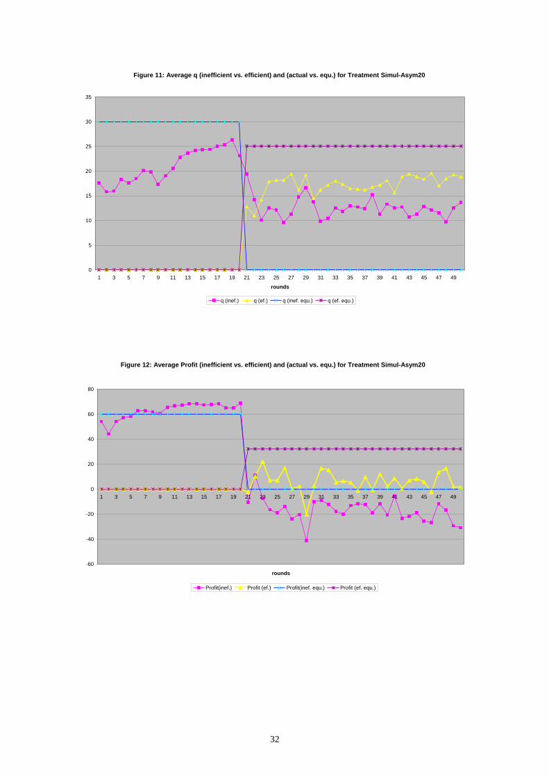
at behavior in the different treatments figures 11 to 12 pertaining to treatment Simul-

Asym20 document that for the case of block entry the length of the incumbency has no

effect on behavior.

Figure 13 presents the ratios of total profits over equilibrium profits for the six

treatments and the four blocks of rounds and figure 14 presents the analogous

information for consumer surplus. Taken together, these two graphs tell a good part of

the story of what goes on in our data. Consumer surplus’ evolution over time is very

similar in the different treatments. It is below equilibrium before entry and then moves

upward. Total profits are, in all but one treatment, a little above equilibrium in the

incumbency phase. After entry they increase in the two treatments with symmetric firms

but decrease and even become negative in the other four treatments.

We now move to a more formal statistical analysis of behaviour. We first study

the overall performance of markets as reflected in consumer surplus and total profit

levels and later move to analyzing incumbents’ behaviour. Table 5 presents the results

of OLS regressions that study the determinants of consumer surplus. The dependent

16

variables are Csi, i=1, 2, 3, 4. The label Cs pertains to the ratio between actual and

equilibrium surplus and the number at the end refers to one of the 10 round blocks,

except for the last two treatments where the block 1 actually had 20 rounds. In the first

four regressions the exogenous variables are – apart from the constant – dummy

variables corresponding to the different (exogenous) treatments. “Short” refers to and

initial incumbency phase of ten rounds and “simul” and “seq” have the same meaning as

in the treatment labels. The notion here is simply to see by comparison between the four

regressions how the exogenous treatments affect behaviour over time. In the last

regressions where the endogenous variables are Cs2, Cs3 and Cs4 we include Cs1 as

exogenous variable to check for any level effect of pre-entry behaviour. In these and all

our other regressions below we take each session as a separate data point. In this way

our regression analysis is based on statistically independent information.

Table 5. Determinants of consumer surplus

Dependent Variable

Cs1 Cs2 Cs3 Cs4 Cs2 Cs3 Cs4

Short .1183341

(.10004235)

-.2516742

(.076677)***

-.1127737

(.0573833)*

-.1075392

(.0669299)

-.2908829

(.0713993)***

-.1190991

(.0590489)

-0927872

(.067955)

Simul .0033156

(.0761754)

.0844986

(.0581626)

.0290225

(.0435276)

-.0811379

(.0507691)

.0834001

(.0531455)

.0288453

(.0439526)

-.0807246

(.0505818)

Sym .1053527

(.0930456)

.0117085

(.0710437)

-.2119034

(.0531675)***

-.0821626

(.0620127)

-.0231989

(.0660594)

-.2175349

(.0546328)***

-.069029

(.0628728)

Cs1 - - - - .3313386

(.1162758)***

.0534537

(.0961629)

-.1246639

(.1106667)

Constant .5046755

(.0791716)***

1.069584

(.0604504)***

1.234489

(.0452397)***

1.157069

(.052766)***

.9023656

(.0805876)***

1.207512

(.0666479)***

1.219984

(.0767001)***

Adjusted

R2 .074 .26 .50 .20 .38 .49 .20

17

The table shows the value of the coefficient and the standard error in

parentheses; negative coefficients indicate a worsening of the attained consumer surplus

with respect to the equilibrium level. The first regression reveals that the collusion that

is present in the first ten rounds is – as expected – independent of treatment; the

strongly significant constant shows that consumer surplus is way below its equilibrium

level; recall that there are no production inefficiency problems in the first rounds.

The next three regressions reflect the impact of the treatment variables over

time. The shorter incumbency phase has a negative impact which weakens over time

both in its magnitude and its significance level. Perhaps surprisingly the simultaneity or

sequentiality of entry has never a significant effect. Symmetry has a significantly

negative effect in rounds 11-20 after the first entry, but no significant effect before and

after that.

Table 6. Determinants of total profits

Dependent Variable

Ps1 Ps2 Ps3 Ps4 Ps2 Ps3 Ps4

Short .0031667

(.0558155)

1.097668

(.1851885)***

.1617356

(.2810005

.1449726

(.4083729)

1.10275

(.164386)***

.1646071

(.2803385)

.1404271

(.4061353)

Simu -.0356655

(.0423383)

-.153357

(.1404731)

-.0461841

(.2131504)

.2838034

(..3097676)

-.0961149

(.1259109)

-.0138444

(.2147243)

.2326096

(.3110779)

Sym -.0841235

(.0517148)

-.2765298

(.171583)

.801211

(.2603559)***

.9853862

(.3783705)**

-.141514

(.1578002)

.8774899

(.2691072)***

.8646363

(.3898641)**

Ps1 - - - - 1.604971

(.4908396)***

.9067497

(.8370617)

-1.435387

(1.212678)

Constant 1.092166

(.0440036)***

.1603451

(.1459983)

.1540921

(.2215343)

-.08929017

(.3219518)

-1.59255

(.5515199)***

-.8362292

(.9405439)

1.48478

(1.362596)

Adjusted

R2 .04 .49 .27 .20 .60 .27 .20

18

Table 6 shows regression results corresponding to total profits (producer

surplus). The variables Psi i=1 2, 3, 4 denote producer surplus as a ratio of equilibrium

producer surplus for the four ten round blocks after entry. In the first regression one can

see that initial profits are somewhat above equilibrium and that they are not affected by

any of the treatment variables. The next three regressions reflect the evolution of profits

over time. A shorter incumbency phase actually helps keeping profits up (in a way, an

anti-inertia result). The symmetry dummy has a significantly positive effect on Ps3 and

Ps4. Inspecting again figures x and y above helps interpret this finding. In the

asymmetric cases incumbent firms frequently resist leaving the market even if this

implies negative profits.

The last three regressions in table 6 reveal that the effects of the treatment

variables are essentially not affected by the inclusion of Ps1 as exogenous variable,

which does have a positive effect in the first ten rounds after entry.

We now move to studying more formally incumbents’ output decisions. In table

7 we can see the impact of the treatment variables on the variables denoted by

Msdi=((incumbents’ profits/total profits) – (incumbents’ equilibrium profits/total

equilibrium profits)), i=1, 2, 3, where Msd is an acronym for market share difference.

The subscript refers here to blocks of rounds after the incumbency phase, since during

this phase Msd is by definition zero. In equilibrium this variable is always equal to one,

positive values correspond to incumbents being able to hold on to market share after

entry. The first three regressions’ exogenous variables are again the treatment variables,

in the last three regressions we condition on Ps1, a measure of collusion in the

incumbency phase.

19

Table 7. Incumbents’ market share deviations from equilibrium

Dependent variable

Msd1 Msd2 Msd3 Msd1 Msd2 Msd3

Short -.2780945

(.0590547)***

.1289026

(.0598136)**

-.0116774

(.0654898)

-.2789681

(.0578234)***

.1279074

(.0579978)**

-.0125552

(.0645416)

Simul .0234117

(.0447954)

.0029767

(.0453711)

.0409028

(.0496767)

.0135728

(.0442896)

-.0082312

(.0444232)

-0310167

(.0494354)

Sym -.0873784

(.0547161)

-.4781715

(.0554192)***

-.2667021

(.0606784)***

-.1105851

(.0555068)*

-.5046073

(.0556742)***

-.2900203

(.0619558)***

Ps1 - - - -.258647

(.172645)

-.3142496

(.1731754)*

-.2771904

(.1927144)

Constant .3529608

(.0465574)***

..3299283

(.047155/)***

.2815486

(.0516306)***

.6542508

(.193999)***

.6731411

(.1945843)***

.5842865

(.2165388)**

Adjusted R2 .54 .68 .41 .56 .70 .43

Here we can see that symmetry has a significantly negative impact on the Msd

variable. Consistent with what we have seen above, in the asymmetric treatments the

incumbents are able to maintain larger than equilibrium market shares to a statistically

significant degree. The length of the incumbency phase also has a statistically

significant impact, negative in the first ten post-entry rounds and positive in the second

ten post-entry rounds.

We can now formulate four regularities which are answers to the four research

questions that we posed in section 2.1. In the concluding section we discuss their

implications.

20

Regularity 1: When firms are identical consumer and total surplus reach equilibrium levels after enough entry. When incumbents are less efficient than entrants consumer surplus tend to equilibrium but total surplus remains considerably below equilibrium. These results are independent of whether entry is sequential or simultaneous and of the length of the incumbency phase. Regularity 2: When firms are identical incumbents are not able to hold on to a larger than equilibrium market share. When incumbents are less efficient than entrants, incumbents’ post-entry actual market shares are significantly larger than in equilibrium. Regularity 3: Whether entry is simultaneous or sequential has no effect on consumer surplus, total surplus and incumbent market shares? Regularity 4: A shorter incumbency phase leads to lower consumer surplus and higher profits in rounds 21-30 after first entry. It has a significantly negative impact on incumbents’ market in rounds 11-20 and to a significantly positive impact in rounds 21-30.

4. Concluding remarks

We can now get back to the major themes that we presented in the introduction

to the paper. The experiments we present in this paper are meant to be a contribution to

the understanding of the market selection process. We find that in the different

treatments with asymmetric firms incumbents produce significantly more and entrants

significantly less of what the relevant equilibrium prescribes. Consistent with this, profit

levels in these markets is substantially below equilibrium. For the incumbents this can

be seen as a purely tactical action to try to limit the entrants’ market share, since they do

not have any strategic advantage in terms of an entry cost or any other factor.

The replacement of inefficient firms by more efficient ones is, in our

environment, not a clean process; it takes place with some turbulence. This is perhaps

the main idea to take away from our work: market selection of more efficient firms

works eventually, but during a certain transition phase some of the agents in the market

will oppose resistance to market forces and by doing it distort market signals.

21

It is interesting that in the symmetric markets of our treatments with symmetric

firms we do not observe significant incumbency advantages. This suggests that

observed behavior in the asymmetric markets is not just the result of incumbents having

“deep pockets” due to the accumulated earnings from the duopoly phase. There is

something in the characteristics of the asymmetric equilibrium that is difficult for

participants to gauge or accept. One possibility is that in the experiment incumbents

resisted obtaining lower payments in the experimental currency. However, we used

different conversion rates for participants with different entry points. Also, when entry

occurs incumbents have had an incumbency phase behind them in which they have been

able to accumulate earnings, so that from the point of view of relative payoffs

incumbents should not necessarily feel as being behind. We feel that instead

incumbents’ behavior is driven by some sense of entitlement and the fact that

accumulated earnings make their costly resistance more bearable.

The incumbency advantage that we observe does not hurt consumers. The fights

for the market between incumbents and entrants lead to large output levels and low

prices. However, production inefficiencies are considerable and lead to total surplus

levels of about 80% of the equilibrium levels.

The fact that incumbents often earn negative profits when they behave in such a

way indicates that it will not be sustainable in the long-run. We conjecture that after

enough time behavior will resemble rather closely the one corresponding to the Cournot

equilibrium. Nevertheless, the behavior we observe does not appear to be a simple

anomaly of the very short run.

22

REFERENCES

Abbink, K., J. Brandts and T.M. McDaniel (2003), “Asymmetric demand information in uniform and discriminatory call auctions: an experimental analysis motivated by electricity markets”, Journal of Regulatory Economics, 23, 125-144. Bain, J. (1956), Barriers to New Competition, Cambridge: Harvard University Press. Basu, K. (1993), Lectures in Industrial Organization Theory, Blackwell Publishers, Oxford. Borenstein, S. and J. Bushnell (1999), “An Empirical Analysis of the Potential for Market Power in California’s Electricity Industry”, Journal of Industrial Economics, 47, 285-??? Brandts, J., A. Cabrales and G. Charness (forthcoming), “Entry Deterrence and Forward Induction: An Experiment”, Economic Theory. Brandts, J. and D. Cooper (2006), “A Change Would Do You Good: An Experimental Study of How to Overcome Coordination Failure in Organzations”, American Economic Review, 96, 669-693. Brandts, J., P. Pezanis-Christou and A. Schram (forthcoming), “Competition with Forward Contracts: A Laboratory Analysis Motivated by Electricity Market Design”, Economic Journal. Bresnahan, T. And P. Reiss (1991), “Entry and Competition in Concentrated Markets”, Journal of Political Economy, 99, 977-1009. Borenstein, S. And J. Bushnell (1999), “An Empirical Analysis of the Potential for Market Power in a deregulated California Electricity Industry”, Journal of Industrial Economics, 47, 285-323. Caves, R. (1998), “Industrial Organization and New Findings on the Turnover and Mobility of Firms”, Journal of Economic Literature, 36, 1947-1982. Ericson, R. and A. Pakes (1995), “Markov-perfect Industry Dynamics: A Framework for Empirical Work”, Review of Economic Studies, 62, 53-82. Fischbacher, U. (1999), "Z-tree. Zurich Toolbox for Readymade Economics Experiments - Experimenter's Manual", Working Paper No. 21, Institute for Empirical Research in Economics, University of Zurich. Holt, C. (1995), “Industrial Organization: A Survey of Laboratoryy Research”, in The Handbook of Experimental Economics, ed. By J. Kagle and A. Roth, Princeton Univesity Press, Princeton, N.J.. Hopenhayn, H. (1992), “Entry, Exit and Firm Dynamics in Long Run Equilibrium”, Econometrica 60, 1127-1150. Huck, S., H-T. Normann and J. Oechssler, Jörg (2004), “Two are few and four are many: Number effects in experimental oligopoly, Journal of Economic Behavior and Organization 53, 435-446. Isaac. R. and V. Smith (1985), “In Search of Predatory Pricing”, Journal of Political Economy, 93, 320-345. Jovanovic, B. (1982), “Selection and the Evolution of Industry”, Econometrica, 50, 649-670.

23

Jung, Y., J. Kagel and D. Levin (1994), “On the existence of predatory pricing. An experimental study of reputation effects in a chain store game”, RAND Journal of Economics, 25, 72-93. Kerin, R., R. Varadarajan and R. Peterson (1992), “First-mover advantage: A synthesis, conceptual framework, and research propositions”, Journal of Marketing, 56, 33-52. Lieberman, M. And D. Montgomery (1988), “First-mover advantages”, Strategic Management Journal, 9, 41-58. Lieberman, M. And D. Montgomery (1998), “First-mover (dis)advantages: Retrospective and Link with the resource-based view”, Strategic Management Journal, 19, 1111-1125. Martin, Stephen (1993), Advanced Industrial Economics, Basil Blackwell. Mueller, D. (1997), “First-mover advantage and path dependence”, International Journal of Industrial Organization, 15, 827-850. Muller, R. and A. Sadanand (2003), “Order of Play, Forward Induction, and Presentation Effects in Two-Person Games”, Experimental Economics, 6, 5-25. Normann, H.-T. and R. Ricciuti (2004), “Experiments for Policy Making”. Opinion Paper for the Economics Network for Competition and Regulation. Plott, C. (1997), “Laboratory Experimental Testbed. Application to the PCS Auction”, Journal of Economics and Management Strategy, 6, 605-638. Plott, C. and T. Salmon (2004), “The Simultanous, Ascending Auction: Dynamics of Price Adjustment in Experiments and in the U.K. 3G Spectrum Auction”, Journal of Economic Behavior and Organization, 53, 353-383. Rapoport, A. (1997), “Order of Play in Strategically-equivalent Games in Extensive Form”, International Journal of Game Theory, 26, 113-136. Rapoport, A., D. Budescu, and R. Suleiman (1993), “Sequential Requests from Randomly-distributed Shared Resources”, Journal of Mathematical Psychology, 37, 241-265. Rapoport, A., E. Weg, and D. Felsenthal (1990), “Effects of Fixed Costs in Two-person Sequential Bargaining”, Theory and Decision, 28, 47-71. Rassenti, S., V. Smith and B. Wilson (2003), “Controlling Market Power and Price Spikes in Electricity Networks: demand-side bidding”, Proceedings of the National Academy of Science, 100, 5, 2998-3003. Rassenti, S., V. Smith and B. Wilson (2001), “Discriminatory Price Auctions in Electricity Markets: Low Volatility at the Expense of High Price Levels”, WP, University of Arizona, December 2001. Rassenti, S., V. Smith and B. Wilson (2002), “Using experiments to Inform the Privatization/Deregulation Movement in Electricity”, The Cato Journal, 22, 3, winter 2002. Roberts, M. and J. Tybout (1997), “Producer Turnover and Productivity Growth in Developing Countries”, World Bank Research Observer, 12, 1-18.

24

Robinson, W. G. Kalyanaram and G. Urban (1994), First-mover advantages from pioneering new markets: A survey of empirical evidence”, Review of Industrial Organization, 9, 1-23. Sylos-Labini, P. (1962), Oligopoly and Technical Progress, Cambridge: Harvard University Press. Tirole, J. (1989), The Theory of Industrial Organization, MIT Press, Cambridge MA. Vives, X. (1999), Oligopoly Pricing: Old Ideas and New Tools, MIT Press, Cambridge MA. Weber, R., C. Camerer and M. Knez (2004), “Timing and Virtual Observability in Ultimatum Games and ‘Weak Link’ Coordination Games”, Experimental Economics, 7, 25-48. Zhang, S., S. Nash and D. Bickford (1995), “Transforming technological pioneering into competitive advantage”, Academy of Management Executive. 9, 17-31..

25

Table 3. Total Quantity (actual vs. equilibrium) TREATMENT

Seq-Sym10 TREATMENT Simul-Sym10

TREATMENT Seq-Asym10

TREATMENT Simul-Asym10



Period Q(equ.) Q(actual)

Q (equ.) Q (actual)

Q (Equ.) Q (Actual)

Q (equ.) Q (actual)

Q (equ.) Q (actual)

Q (equ.) Q (actual)

1 40 31,13 40 22,79 60 41,8 60 27,83 60 37 60 35,172 40 34 40 24,55 60 47,4 60 28,17 60 42 60 31,673 40 31,63 40 26,55 60 46 60 37,5 60 47,33 60 324 40 31,75 40 29,33 60 42,6 60 40,67 60 44,67 60 36,675 40 31,13 40 33 60 46,6 60 40 60 44,17 60 35,176 40 32,63 40 35,33 60 45 60 41,83 60 43,83 60 377 40 33,38 40 35,44 60 41,8 60 47,5 60 45,5 60 40,178 40 33,75 40 38,22 60 46 60 49 60 46,83 60 39,679 40 36,25 40 37,67 60 49,6 60 47,67 60 44,33 60 34,6710 40 37,5 40 36,33 60 43,8 60 43,33 60 45,33 60 38,1711 45 49,75 50 59,99 70 63,6 75 78 60 47 60 41,1712 45 36,38 50 44,77 70 54,6 75 74,83 60 50,33 60 45,513 45 33,88 50 40,65 70 61,4 75 65 60 48,67 60 47,314 45 38,5 50 43,45 70 65,2 75 72,5 60 48,33 60 48,3315 45 40,15 50 48,88 70 57,8 75 61,33 60 48,33 60 48,6716 45 36,25 50 43,45 70 66,6 75 74,67 60 47 60 48,8317 45 38 50 47,99 70 70,4 75 73,5 60 49,5 60 5018 45 39,13 50 44,33 70 63 75 79,67 60 50 60 50,6719 45 37,38 50 45,78 70 62,4 75 72,33 60 49,5 60 52,6720 45 38,88 50 50,78 70 60,6 75 71,67 60 52,5 60 46,3321 48 44,88 50 49,23 66 65,4 75 75 70 55,33 75 77,3322 48 39,75 50 47 66 63,4 75 72,17 70 52,5 75 61,3323 48 44,13 50 46,55 66 72,6 75 70,67 70 58,5 75 62,6724 48 44 50 48,21 66 77,8 75 73 70 60,67 75 78,525 48 41,25 50 50,22 66 76,6 75 70,5 70 62,17 75 7926 48 47,13 50 51 66 67 75 75,17 70 62 75 73,6727 48 43,3 50 50,89 66 61,6 75 75,67 70 62,83 75 81,1728 48 48,75 50 44,43 66 69,6 75 70 70 64 75 7829 48 48,13 50 47,23 66 66,4 75 76,67 70 66,33 75 9130 48 45,17 50 47,21 66 77,2 75 76,67 70 68,17 75 70,8331 50 47,38 50 47,54 75 88,8 75 78,5 66 78,17 75 68,3332 50 50 50 47,21 75 72,8 75 76,33 66 70 75 72,533 50 44,13 50 50,65 75 75,8 75 79 66 66,33 75 7934 50 45,1 50 47,45 75 77,8 75 73,67 66 69,33 75 75,8335 50 50,07 50 49,98 75 72,6 75 78,67 66 67,83 75 75,3336 50 52,25 50 43,9 75 83 75 82,5 66 73,33 75 74,537 50 51,88 50 44,32 75 77,6 75 83,67 66 75,5 75 73,6738 50 45,13 50 44,95 75 76,6 75 80 66 63,5 75 80,8339 50 48,75 50 44,21 75 85,6 75 77,83 66 66 75 74,3340 50 44,75 50 45,74 75 88,8 75 76 66 69,67 75 8141 75 71,17 75 72,1742 75 68 75 82,1743 75 68,67 75 8044 75 70 75 79,3345 75 75,17 75 80,8346 75 70,83 75 83,1747 75 71,67 75 74,1748 75 68,83 75 74,8349 75 66,33 75 83,1750 75 71,5 75 83,83

26

Table 4. Total Surplus (actual vs. equilibrium) TREATMENT

Seq-Sym10 TREATMENT Simul-Sym10





Period TS (equ.)

TS (actual)

TS (equ.)

TS (actual)

TS (equ.)

TS (actual)

TS (equ.)

TS (actual)

TS (equ.)

TS (actual)

TS (equ.)

TS (actual)

1 290 246,62 290 191,54 300 228,84 300 79,79 300 204,55 300 128,252 290 262,4 290 204,37 300 254,26 300 83,21 300 229,8 300 112,53 290 249,49 290 218,15 300 248,2 300 132,3 300 253,98 300 1144 290 250,19 290 235,96 300 232,66 300 150,27 300 242,24 300 1355 290 246,62 290 257,1 300 250,82 300 145,87 300 239,97 300 128,256 290 255,06 290 269,16 300 243,75 300 152,58 300 238,43 300 136,57 290 259,11 290 269,70 300 228,84 300 178,45 300 245,99 300 150,758 290 261,09 290 282,57 300 248,2 300 187,83 300 251,83 300 148,59 290 273,59 290 280,12 300 263,39 300 173,92 300 240,73 300 12610 290 279,38 290 273,99 300 238,28 300 159,17 300 245,24 300 141,7511 292,5 304,49 275 285 325 300,15 378,75 285,93 300 252,55 300 155,2512 292,5 259,19 275 261,81 325 272,94 378,75 262,73 300 266,33 300 174,7513 292,5 246,75 275 247,57 325 295,70 378,75 218,33 300 259,58 300 18314 292,5 268,78 275 257,61 325 309,05 378,75 260,56 300 258,19 300 187,515 292,5 275,6 275 272,62 325 285,36 378,75 205,8 300 258,19 300 18916 292,5 258,59 275 257,6 325 311,42 378,75 269,98 300 252,55 300 189,7517 292,5 266,6 275 270,57 325 319,59 378,75 271,46 300 262,99 300 19518 292,5 271,42 275 260,45 325 299,15 378,75 298,45 300 265 300 19819 292,5 263,81 275 264,78 325 298,71 378,75 261,28 300 262,99 300 20720 292,5 270,37 275 276,5 325 292,78 378,75 258,02 300 274,69 300 178,521 285,6 277,12 275 273,39 383,1 287,74 378,75 279,42 325 370,4 378,75 293,2922 285,6 258,99 275 268,1 383,1 281,22 378,75 263,75 325 354,44 378,75 212,2923

285,6 274,79

8 275 266,91 383,1 311,26 378,75 252,46 325 385,19 378,75 217,2624 285,6 274,4 275 271,10 383,1 318,76 378,75 260,14 325 390,79 378,75 301,3625 285,6 264,84 275 275,44 383,1 316,82 378,75 246,02 325 396,17 378,75 304,3526 285,6 283,42 275 276,90 383,1 296,75 378,75 278,77 325 410,73 378,75 275,2327 285,6 272,08 275 276,69 383,1 283,67 378,75 281,22 325 396,6 378,75 319,3328 285,6 287,34 275 260,76 383,1 302,19 378,75 249,13 325 383,83 378,75 299,1429 285,6 285,9 275 268,70 383,1 295,15 378,75 288,31 325 393,26 378,75 373,3830 285,6 288 275 268,65 383,1 322,01 378,75 289,65 325 400,6 378,75 264,1431 275 269,06 275 269,48 378,75 322,73 378,75 297,27 383,1 329,57 378,75 248,4832 275 275 275 268,64 378,75 292,81 378,75 287,36 383,1 322,92 378,75 269,3233 275 259,8 275 276,27 378,75 296,92 378,75 297,13 383,1 312,41 378,75 304,8134 275 262,8 275 269,24 378,75 302,56 378,75 270,81 383,1 327,8 378,75 289,0835 275 275,14 275 274,96 378,75 291,26 378,75 298,50 383,1 319,55 378,75 285,9736 275 278,99 275 259,09 378,75 308,35 378,75 319,43 383,1 324,33 378,75 285,2837 275 278,4 275 260,41 378,75 300,11 378,75 322,83 383,1 339,05 378,75 276,138 275 262,87 275 262,36 378,75 305,02 378,75 304,76 383,1 315,47 378,75 314,2739 275 272,34 275 260,07 378,75 320,83 378,75 295,4 383,1 324,75 378,75 279,340 275 261,74 275 264,65 378,75 320,33 378,75 281,68 383,1 330,38 378,75 315,6141 378,75 285,27 378,75 268,942 378,75 273,97 378,75 322,843 378,75 283,08 378,75 310,7444 378,75 285,83 378,75 306,1245 378,75 295,33 378,75 313,3446 378,75 283,8 378,75 329,7647 378,75 285,86 378,75 277,5848 378,75 282,43 378,75 281,0349 378,75 275,16 378,75 327,3350 378,75 288,89 378,75 329,73

27

Figure 1: Average q across firm groups for Treatment Seq-Sym10

0

2

4

6

8

10

12

14

16

18

20

1 2 3 4 5 6 7 8 9 10 11 12 13 14 15 16 17 18 19 20 21 22 23 24 25 26 27 28 29 30 31 32 33 34 35 36 37 38 39 40

q1-q2 q3 q4 q5

Figure 2: Average q (incumbents vs. entrants) for Treatment Simul-Sym10

0

5

10

15

20

25

1 2 3 4 5 6 7 8 9 10 11 12 13 14 15 16 17 18 19 20 21 22 23 24 25 26 27 28 29 30 31 32 33 34 35 36 37 38 39 40

rounds

q12(actual) q (potentials)

28

Figure 3: Average q across firm groups for Treatment Seq-Asym10

0

5

10

15

20

25

30

1 2 3 4 5 6 7 8 9 10 11 12 13 14 15 16 17 18 19 20 21 22 23 24 25 26 27 28 29 30 31 32 33 34 35 36 37 38 39 40

rounds

average q12 q(3) q(4) q(5)

Figure 4: Average q (inefficient vs. efficient) and (actual vs. equ.) for Treatment Seq-Asym10

0

5

10

15

20

25

30

35

1 2 3 4 5 6 7 8 9 10 11 12 13 14 15 16 17 18 19 20 21 22 23 24 25 26 27 28 29 30 31 32 33 34 35 36 37 38 39 40

rounds

average q12 average q (ef.) Equ q(inef.) Equ. q (ef.)

29

Figure 5: Average profit (inefficient vs. efficient) for Treatment Seq-Asym10

-40

-20

0

20

40

60

80

1 2 3 4 5 6 7 8 9 10 11 12 13 14 15 16 17 18 19 20 21 22 23 24 25 26 27 28 29 30 31 32 33 34 35 36 37 38 39 40

rounds

Profit inefficient Profit efficient

Figure 6: Average q (inefficient vs. efficient) and (actual vs. equ.) for Treatment Simul-Asym10

0

5

10

15

20

25

30

35

1 2 3 4 5 6 7 8 9 10 11 12 13 14 15 16 17 18 19 20 21 22 23 24 25 26 27 28 29 30 31 32 33 34 35 36 37 38 39 40

rounds

q(inef.) q(ef.) q (inef. equ.) q (ef. equ.)

30

Figure 7: Average Profit (inefficient vs. efficient) for Treatment Simul-Asym10

-40

-20

0

20

40

60

80

1 2 3 4 5 6 7 8 9 10 11 12 13 14 15 16 17 18 19 20 21 22 23 24 25 26 27 28 29 30 31 32 33 34 35 36 37 38 39 40

rounds

Profit(inef.) Profit(ef.)

Figure 8: Average q across firm groups for Treatment Seq-Asym20

0

5

10

15

20

25

30

35

1 3 5 7 9 11 13 15 17 19 21 23 25 27 29 31 33 35 37 39 41 43 45 47 49

rounds

q1 q2 q3 q4 q5

31

Figure 9: Average q (inefficient vs. efficient) and (actual vs. equ.) for Treatment Seq-Asym20

0

5

10

15

20

25

30

35

1 3 5 7 9 11 13 15 17 19 21 23 25 27 29 31 33 35 37 39 41 43 45 47 49

rounds

q(inef) q(ef.) q(inef. equ.) q(ef. equ.)

Figure 10: Average Profits (inefficient vs. efficient) for Treatment Seq-Asym20

-20

-10

0

10

20

30

40

50

60

70

80

1 3 5 7 9 11 13 15 17 19 21 23 25 27 29 31 33 35 37 39 41 43 45 47 49

rounds

Profit (inef.) Profit (ef.)

32

Figure 11: Average q (inefficient vs. efficient) and (actual vs. equ.) for Treatment Simul-Asym20

0

5

10

15

20

25

30

35

1 3 5 7 9 11 13 15 17 19 21 23 25 27 29 31 33 35 37 39 41 43 45 47 49

rounds

q (inef.) q (ef.) q (inef. equ.) q (ef. equ.)

Figure 12: Average Profit (inefficient vs. efficient) and (actual vs. equ.) for Treatment Simul-Asym20

-60

-40

-20

0

20

40

60

80

1 3 5 7 9 11 13 15 17 19 21 23 25 27 29 31 33 35 37 39 41 43 45 47 49

rounds

Profit(inef.) Profit (ef.) Profit(inef. equ.) Profit (ef. equ.)

33

Figure 13: TP(actual) / TP(equ) ratio across treatments

-0,5

0

0,5

1

1,5

2

2,5

3

1 2 3 4

Round Blocks

Seq-Sym10 Simul-Sym10 Seq-Asym10 Seq-Asym20 Simul-Asym10 Simul-Asym20

Figure 14: CS(actual) / CS(equ) ratio across treatments

0

0,2

0,4

0,6

0,8

1

1,2

1,4

1 2 3 4

Round Blocks

Seq-Sym10 Simul-Sym10 Seq-Asym10 Seq-Asym20 Simul-Asym10 Simul-Asym20

34

APPENDIX: INSTRUCTIONS FOR TREATMENT 2.1a

General Information. We thank you for coming to the experiment. The purpose of this session is to study how people

make decisions in a particular situation. During the session it will not be permitted to talk or communicate with the other participants. If you have a question, please raise your hand and one of us will come to your table to answer it. During the session you will earn money. During the session the income will be denominated in points. At the end of the session the points will be converted into euros in a way that is explained below. At the end of the session the amount you have earned will be paid to you in cash. Payments are confidential, we will not inform any of the other participants of the amount that you earn. Groups and types in groups. During the experiment you will be in a group of five, you and another four participants. Each group will be composed by the same five persons during the whole experiment. The members of each group will be of different types: A, B, C, D and E. Types A and B will be in one situation, type C will be in a different situation, type D in a different situation, and type E in again a different situation. The composition of the groups and the types within the groups will be determined randomly. Periods. The session consists of 40 periods. In periods 1 to 10 the types A and B of each group will make decisions and the types C, D and E will not make decisions. After each of the periods 1 to 10 all the types in one group will receive information about the decisions made by the A and B in the group. In periods 11 to 20 types A, B and C of each group will make decisions and types D and E will not make decisions. After each of the periods 11 to 20 all the types in one group will receive information about the decisions made by the A, B and C in the group.

In periods 21 to 30 types A, B, C and D of each group will make decisions and type E will not make decisions. After each of the periods 21 to 30 all the types in one group will receive information about the decisions made by the A, B, C and D in the group.

In periods 31 to 40 types A, B, C, D and E of each group all will make decisions. After each of the periods 31 to 40 all the types in one group will receive information about the decisions made by the A, B, C, D and E in the group. Period 40 will be the last of the session.

Decisions and periods Periods Types that make decisions Types that don’t make

decisions 1-10 A y B C, D y E

11-20 A, B y C D y E 21-30 A, B, C y D E 31-40 A, B, C, D y E -

Decisions and earnings. When somebody has the possibility of making a decision, this decision will consist in which quantity to produce to sell in a market. Any integer quantity between 0 and 30 can be chosen. In periods 1 to 10, types A and B of each group will have to decide individually which quantity to produce. Participants C, D and E will not make decisions and their earnings in these periods will be zero. The earnings of each period for A and B will depend on their decisions. If type A or B produces zero in a period his earnings in that period will be zero. If he produces a positive quantity then the earnings will be Earnings = (Price –MC)*quantity produced by the participant – F, MC = 2. This is called “marginal cost” and is paid for each produced unit.

35

F=30. This is called “fixed cost”. It is a fixed quantity which will be subtracted any time that the quantity produced by the participant is positive. The price depends on the sum of the quantities produced by types A and B. To see what prices correspond to the different sums of quantities see the table on the next page. Observe that the larger the sum of quantities produced by A and B the lower the price. If the resulting price is very low or negative the earnings from the period can be negative

TOTAL QUANTITY PRODUCED

PRICE TOTAL QUANTITY PRODUCED

PRICE TOTAL QUANTITY PRODUCED

PRICE

1 10.9 41 6.9 81 2.9 2 10.8 42 6.8 82 2.8 3 10.7 43 6.7 83 2.7 4 10.6 44 6.6 84 2.6 5 10.5 45 6.5 85 2.5 6 10.4 46 6.4 86 2.4 7 10.3 47 6.3 87 2.3 8 10.2 48 6.2 88 2.2 9 10.1 49 6.1 89 2.1

10 10 50 6 90 2 11 9.9 51 5.9 91 1.9 12 9.8 52 5.8 92 1.8 13 9.7 53 5.7 93 1.7 14 9.6 54 5.6 94 1.6 15 9.5 55 5.5 95 1.5 16 9.4 56 5.4 96 1.4 17 9.3 57 5.3 97 1.3 18 9.2 58 5.2 98 1.2 19 9.1 59 5.1 99 1.1 20 9 60 5 100 1 21 8.9 61 4.9 101 0.9 22 8.8 62 4.8 102 0.8 23 8.7 63 4.7 103 0.7 24 8.6 64 4.6 104 0.6 25 8.5 65 4.5 105 0.5 26 8.4 66 4.4 106 0.4 27 8.3 67 4.3 107 0.3 28 8.2 68 4.2 108 0.2 29 8.1 69 4.1 109 0.1 30 8 70 4 110 0 31 7.9 71 3.9 111 -0.1 32 7.8 72 3.8 112 -0.2 33 7.7 73 3.7 113 -0.3 34 7.6 74 3.6 114 -0.4 35 7.5 75 3.5 115 -0.5 36 7.4 76 3.4 116 -0.6 37 7.3 77 3.3 117 -0.7 38 7.2 78 3.2 118 -0.8 39 7.1 79 3.1 119 -0.9 40 7 80 3 120 -1

36

In periods 11 to 20, types A, B and C of each group will have to decide individually which quantity to produce. Participants D and E will not make decisions and their earnings in these periods will be zero. The earnings of each period for A, B and C will depend on their decisions. If type A, B or C produces zero in a period his earnings in that period will be zero. If he produces a positive quantity then the earnings will be: Earnings = (Price –MC)*quantity produced by the participant – F, MC = 2. This is called “marginal cost” and is paid for each produced unit. with MC = 2 and F=30 as before for types A and B, and MC=1 and F=30 for type C. The price now depends on the sum of the quantities produced by types A, B and C, following the same table as before. If the resulting price is very low or negative the earnings from the period can be negative.

In periods 21 to 30, types A, B, C and D of each group will have to decide individually which quantity to produce. Participant E will not make decisions and his earnings in these periods will be zero. The earnings of each period for A, B, C and D will be determined by the same expression as before, with MC=1 and F=30 for type D. The price now depends on the sum of the quantities produced by types A, B, C and D following the same table as before. If the resulting price is very low or negative the earnings from the period can be negative.

In periods 31 to 40, types A, B, C, D and E of each group will have to decide individually which quantity to produce. The earnings of each period for A, B, C, D and E will be determined by the same expression as before, with MC=1 and F=30 for type E. The price now depends on the sum of the quantities produced by types A, B, C, D and E following the same table as before. If the resulting price is very low or negative the earnings from the period can be negative.

Information after each period. After each period you will all be informed of the total quantity produced by the group, of your own production and (in case it applies) of your earnings in points. You will also be informed of your accumulated earnings. Types and identification numbers On your screen you will see your identication number. The participants with identification numbers 1, 6, and 11 will be the types A of each of the groups. The participants with identification numbers 2, 7, and 12 will be the types B of each of the groups. The participants with identification numbers 3, 8, and 13 will be the types C of each of the groups. The participants with identification numbers 4, 9, and 14 will be the types D of each of the groups. The participants with identification numbers 5, 10, and 15 will be the types E of each of the groups. Total earnings. At the beginning of the session each participant will receive and additional endowment of 330 points. After each period the earnings of the period will be added to (or subtracted from) the initial endowment to determine the current earnings in points. At the end of the session the earnings in points will be transformed into euros. The exchange rate will be different for each type. For types A and B each point will be exchanged for 0,021 euros.

For type C each point will be exchanged for 0,019 euros. For type D each point will be exchanged for 0,029 euros. For type E each point will be exchanged for 0,075. euros.

Entry and Market Selection of Firms: A Laboratory...

Documents

Transcript of Entry and Market Selection of Firms: A Laboratory...