BRX-TH-6314

Entanglement shadows in LLM geometries

Vijay Balasubramanian∗a,d, Albion Lawrence†b,Andrew Rolph‡b, and Simon F. Ross§c

a David Rittenhouse Laboratories, University of Pennsylvania209 S 33rd Street, Philadelphia, PA 19104, USA

b Martin Fisher School of Physics,Brandeis University, Waltham, MA 02453, USA

c Centre for Particle Theory, Department of Mathematical SciencesDurham University, South Road, Durham DH1 3LE, UK

d Theoretische Natuurkunde, Vrije Universiteit Brussel (VUB),and International Solvay Institutes, Pleinlaan 2, B-1050 Brussels, Belgium

October 12, 2017

Abstract

We find a new example of an asymptotically AdS5 × S5 geometry which has anentanglement shadow: that is, a region of spacetime which no Ryu-Takayanagi min-imal surface enters. Our example is a particular case of the supersymmetric LLMgeometries. Our results illustrate how minimal surfaces, which holographically ge-ometrize entanglement entropy, can fail to probe the whole of spacetime, posing achallenge for attempts to directly reconstruct holographic geometries from the entan-glement entropies of the dual field theory. We also comment on the relation to previousinvestigations of minimal surfaces localised in the S5 factor of AdS5 × S5.

∗vijay@physics.upenn.edu†albion@brandeis.edu‡andrewrolph@brandeis.edu§s.f.ross@durham.ac.uk

arX

iv:1

704.

0344

8v2

[he

p-th

] 1

1 O

ct 2

017

1 Introduction

The Ryu-Takayanagi proposal [1] and its generalizations provide a map between quan-tum entanglement of spatial regions of a strongly coupled large-N field theory andthe spacetime geometry of its gravitational dual, by relating entanglement entropies toareas of minimal or extremal [2] surfaces. This has led to explicit progress in bulk recon-struction, particularly for linearized perturbations of anti-de Sitter space [3–5]. Thereare also attempts to directly represent the areas of arbitrary surfaces in asymptoticallyAdS spacetimes in terms of new information theoretic observables such as “differentialentropy” [6–8]. All of these efforts explicitly use the geometry and deformations ofextremal surfaces of holographic geometries.

This program is complicated (or enriched, as the reader prefers) by the existenceof entanglement shadows: regions of the bulk spacetime which are not reached by anyminimal or extremal surfaces used to compute entanglement between spatial regionsof the boundary (see, e.g., [9,10]). Holographic geometries with entanglement shadowsrequire additional quantities beyond spatial entanglement in the dual field theory forthe purpose of bulk geometry reconstruction.1 Consider, for example, the conicaldefect spacetimes describing excitations of AdS3. In this case, non-minimal extremalsurfaces enter the entanglement shadow region, and there is a candidate generalizationof spatial entanglement called entwinement which yields quantities dual to the area ofthese surfaces [9, 14,15].

In this work, we will argue that a simple but topologically non-trivial asymptoticallyAdS5 × S5 geometry has an entanglement shadow. Our example is one of the “LLMgeometries” [16], which are holographically dual to 1/2-BPS excitations of N = 4super-Yang Mills theory. These geometries are smooth but topologically complex, andthe map to the dual field theory state is known precisely. From the perspective ofreconstructing bulk geometry from quantities in the dual field theory, one of the mostinteresting aspects of the LLM geometries is that they are inherently 10-dimensional– there is no factorization into an asymptotically AdS5 part and a compact part. Ifthere were such a factorization, we could “compactify” the reconstruction problem toone of just recovering the geometry and fields in the asymptotically AdS factor, butthat is not possible here. In fact, it is known that reconstructing the interior geometryand topology of LLM spacetimes from the dual field theory using just local operatormeasurements would require access to trans-Planckian physics [17, 18]. In particular,around configurations with non-trivial topology there is entanglement between theeffective dynamical degrees of freedom and UV modes that are beyond the Planckscale [19–21].

We will consider an LLM geometry which is approximately AdS5 × S5 in both theasymptotic region and a central region in the spacetime. In our geometry, the S3 radialsections of the asymptotic AdS5 essentially exchange roles with an S3 factor inside theS5 to form the central AdS5 region. In this geometry, we study minimal surfacesanchored at the equator of the S3 on the spacetime boundary; these are expected tobe the deepest minimal surface probes of the geometry, and compute the entanglement

1One might likewise wonder how an entanglement-based program would be extended to the BFSS model[11], which is a quantum-mechanical model with an 11d holographic dual [12,13].

2

entropy of half the field theory with the other half. Because of the exchange of the rolesof the S3 factors which we described above, a surface that partitions the boundary ofAdS in the asymptotic region will partition the S5 in the central region. Making somesystematic approximations, we find that in this central region, the minimal surfacefor a boundary condition which divides the S5 penetrates into the bulk only for aproper radial distance of order one in the central AdS factor. At this distance, thissurface closes off by reaching the pole on the S5. From the point of view of the full LLMgeometry, this implies that essentially the whole of the central IR region is not accessedby boundary-anchored minimal surfaces. This is our shadow region. We then arguethat there is an extremal non-minimal surface, also anchored at the equator of thespacetime boundary, which does enter the shadow region. This is similar situation asfor the conical defects in AdS3 which have an entanglement shadow which is penetratedby non-minimal, but extremal, surfaces [9].

Unlike in AdS3 [14,15] we do not yet have a candidate information theoretic quantitysuch as entwinement that computes the area of a non-minimal extremal surface from theperspective of the dual field theory. The idea in [14,15] was that non-minimal extremalsurfaces (“long” geodesics in that case) were related to entanglement in a partition ofdegrees of freedom of the dual field theory that was not spatially organized. It would beworth understanding whether there is such an interpretation for non-minimal extremalsurfaces in the AdS5 case also. Interesting earlier holographic studies of Yang-Millstheory in the Coulomb branch [22–24] had proposed that a minimal surface whichdivides the S5 part of the boundary of an asymptotically AdS5 × S5 spacetime canbe identified with the entanglement entropy associated to a non-spatial division of thefield theory degrees of freedom. In the context of our geometries, the surfaces describedby [22–24] can be regarded as extremal surfaces in the central AdS5 region, which can beextended into the asymptotic AdS5 region to describe entanglement in a conventionalspatial partition of the UV theory. Our analysis shows that the particular extremalsurfaces studied in [22–24] are not, in fact, the minimal ones that are asymptotic tothe equator of the boundary S5. It would be very interesting to understand whatinformation theoretic quantity is being computed by such extremal surfaces, and alsoby the true minimal surfaces with these boundary conditions.

Our paper is organized as follows. In section 2, we briefly review the LLM geome-tries first constructed in [16], and introduce the examples we consider. In section 3 weconsider extremal surfaces in the central region of our geometries, and explain the rela-tion to the earlier work of [22–24]. In section 4, we argue that the boundary-anchoredminimal surfaces in our spacetime close off on the central S5 without penetrating deepinto the central region. Hence these LLM geometries have entanglement shadows. Insection 5, we discuss the extension to other LLM geometries and the interpretation ofour results.

2 LLM geometries

The 1/2 BPS solutions found by Lin, Lunin and Maldacena (LLM) [16] provide a richclass of asymptotically AdS5 × S5 spacetimes where the geometry can be analyzedanalytically, and for which precise field theory duals are known. We will focus on a

3

simple example in this class, and find the bulk extremal surface whose area computesthe entanglement between halves of the spatial S3, across an equator, in the dual fieldtheory.

The LLM geometries correspond to 1/2 BPS states in N = 4 SYM on S3 × R,where the energy of the state (∆) is equal to the charge (J) under a U(1) subgroupof the SO(6) R-symmetry, ∆ = J . The dual geometries should thus be asymptoticallyAdS5×S5 solutions preserving half the supersymmetry, the SO(4) rotational symmetryon the spatial S3, an SO(4) subgroup of the R-symmetry, and a diagonal R group whichcombines time translation with the U(1) ∈ SO(6) to leave the state invariant. LLMfound that these restrictions fix the form of the geometry up to a single function ofthree coordinates, z(y, x1, x2) [16]. The metric is

ds2 = −h−2(dt+ Vidxi)2 + h2(dy2 + dx21 + dx22) + yeGdΩ2

3 + ye−GdΩ23, (1)

i = 1, 2, where the functions h and G are related to z by

h−2 = 2y coshG, z =1

2tanhG, (2)

and Vi is determined by

y∂yVi = εij∂jz, y(∂iVj − ∂jVi) = εij∂yz. (3)

The geometry is supported by a self-dual five-form; the explicit form of the fieldstrength is not needed here. Note that in these coordinates the length element ds2

has units of length, as do y, x1, x2, while t is a dimensionless quantity.The range of the coordinates is y ∈ (0,∞), xi ∈ (−∞,∞), so this is an upper half

space. The metric and five-form give a solution of the supergravity equations of motionif the function z obeys

∂i∂iz + y∂y

(∂yz

y

)= 0. (4)

The solutions will be smooth if z satisfies the boundary condition z → ±1/2 as y → 0.The general solution of (4) with such boundary conditions was given in [16]. Hencesolutions are specified by giving a colouring of the x1, x2 plane, specifying regions wherez → 1/2, which we will draw in white, and regions where z → −1/2, which we willdraw in black. The regions where z → −1/2 correspond to the first S3, with metricdΩ2

3, shrinking to zero as y → 0, while z → 1/2 corresponds to the second S3, withmetric dΩ2

3, shrinking to zero.Note that the solution is a ten-dimensional geometry, and except in special cases,

it is not possible to straightforwardly perform a Kaluza-Klein reduction to obtain afive-dimensional description; we really need to think about these geometries using aten-dimensional perspective.

2.1 AdS5×S5

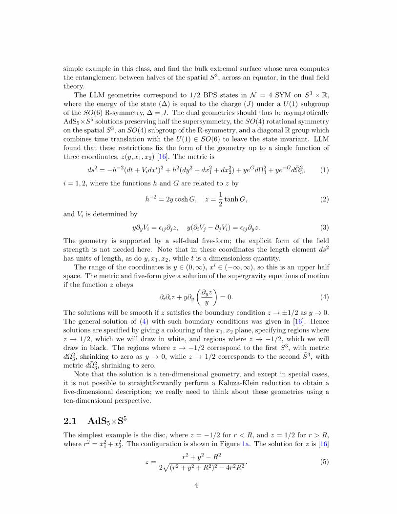
The simplest example is the disc, where z = −1/2 for r < R, and z = 1/2 for r > R,where r2 = x21 +x22. The configuration is shown in Figure 1a. The solution for z is [16]

z =r2 + y2 −R2

2√

(r2 + y2 +R2)2 − 4r2R2. (5)

4

(a) Disk (b) Annulus

Figure 1: LLM configurations in the (x1, x2) plane. The configurations describe boundaryconditions for the equations of motion on a two dimensional surface in the bulk spacetime,and also correspond to configurations in a fermionic phase space that completely summarizesthe boundary 1/2 BPS state. The black disc boundary condition (a) leads to a pure AdS5×S5

geometry. We will show that no entangling surface can probe deeply into the IR region ofthe geometry given by the annulus boundary condition (b).

This corresponds to the vacuum AdS5× S5 solution. If we make the change of coordi-nates

y = R sinh χ sin θ, r = R cosh χ cos θ, φ = φ− t, (6)

where φ is the angular coordinate in the x1, x2 plane, the metric becomes:

ds2 = R(− cosh2 χdt2 + dχ2 + sinh2 χdΩ23 + dθ2 + cos2 θdφ2 + sin2 θdΩ2

3). (7)

The first three terms describe the metric on AdS5 with AdS radius R; the last threeterms describe the metric on S5 with constant radius R.

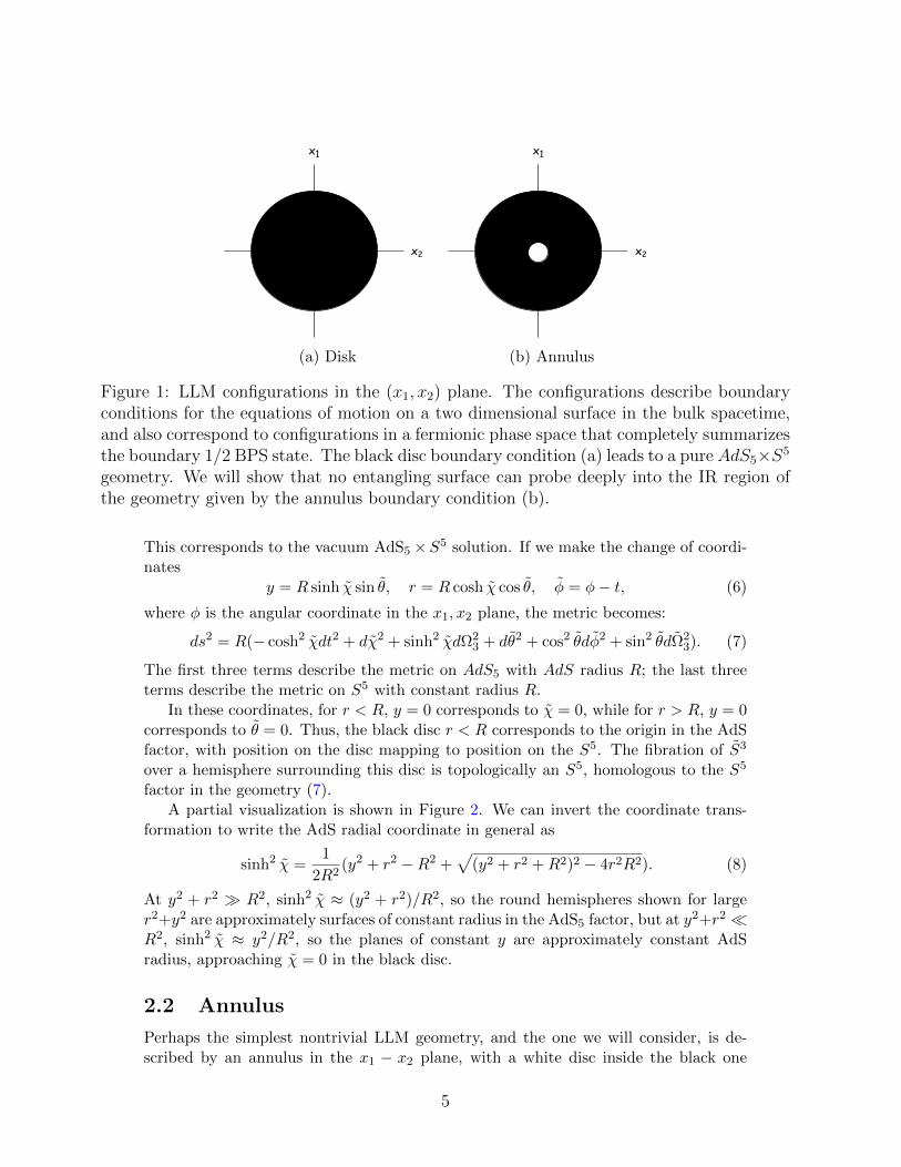
In these coordinates, for r < R, y = 0 corresponds to χ = 0, while for r > R, y = 0corresponds to θ = 0. Thus, the black disc r < R corresponds to the origin in the AdSfactor, with position on the disc mapping to position on the S5. The fibration of S3

over a hemisphere surrounding this disc is topologically an S5, homologous to the S5

factor in the geometry (7).A partial visualization is shown in Figure 2. We can invert the coordinate trans-

formation to write the AdS radial coordinate in general as

sinh2 χ =1

2R2(y2 + r2 −R2 +

√(y2 + r2 +R2)2 − 4r2R2). (8)

At y2 + r2 R2, sinh2 χ ≈ (y2 + r2)/R2, so the round hemispheres shown for larger2+y2 are approximately surfaces of constant radius in the AdS5 factor, but at y2+r2 R2, sinh2 χ ≈ y2/R2, so the planes of constant y are approximately constant AdSradius, approaching χ = 0 in the black disc.

2.2 Annulus

Perhaps the simplest nontrivial LLM geometry, and the one we will consider, is de-scribed by an annulus in the x1 − x2 plane, with a white disc inside the black one

5

Figure 2: A hemisphere over a black disc in the (x1, x2) plane. An S3 fibration over thissurface is topologically an S5.

(Figure 1b). That is, we take the boundary conditions for the function z to bez(y = 0, r > R) = 1

2 , z(y = 0, R > r > ε) = −12 , and z(y = 0, r < ε) = 1

2 . Thesolution is then

z =1

2− y2

π

∫ R

ε

r′dr′dφ′

[r2 + r′2 − 2rr′ cosφ′ + y2]2(9)

=1

2+

1

2

r2 + y2 −R2√(r2 + y2 +R2)2 − 4r2R2

− 1

2

r2 + y2 − ε2√(r2 + y2 + ε2)2 − 4r2ε2

. (10)

The physical picture of this configuration is that it represents the back-reactedversion of maximal giant gravitons [25]. We consider a set of D3-branes wrapping theS3 inside S5 at θ = π/2 where this S3 has maximal volume, with angular momentumalong φ corresponding to the R-charge. These D-branes dissolve into the backreactedgeometry. Note that because of the angular momentum, the annulus geometry isstationary but not static.

2.3 Approximating the annulus geometry

Extremal surfaces in the annulus geometry are in general complicated, and findingthem involves solving a nonlinear PDE in two variables. To make the problem moretractable, we will consider the case where ε R, so that the white hole in the centerof Fig. 1b is small compared to the area of the outer disk. We will still consider thecase that both radii are large compared to the string or Planck scales. The result is aseparation of scales that leads to a straightforward picture of the geometry.

To begin with, we can consider the coordinates at “large” radius, for which r2+y2 εR. In this case, the white disk in the center will appear small and we expect thegeometry to be a small perturbation of an AdS5×S5 geometry with radius of curvatureR. More precisely, the last term in (10) can be approximated by a series expansion inε2/(r2 + y2), which at leading order gives

z ≈ 1

2

r2 + y2 −R2√(r2 + y2 +R2)2 − 4r2R2

+ε2y2

(r2 + y2)2. (11)

6

The corresponding geometry is the AdS5 × S5 metric (7) with a subleading correctionwhich decays at large distances. We call this the “UV AdS region”.

On the other hand, if we consider small distances r2 + y2 εR, the geometry iswell approximated by a black plane with a white disk in the center. Now the LLMgeometries are symmetric under z = 1

2 → −12 while exchanging S3 and S3; thus, the

region is well approximated by AdS5 × S5 with radius of curvature ε, which we dubthe “IR AdS region”. More precisely, the second term in (10) can be expanded in aseries in 1/R2, which gives

z ≈ −1

2

r2 + y2 − ε2√(r2 + y2 + ε2)2 − 4r2ε2

+y2

R2. (12)

The final term in (12) gives a correction to IR AdS which decays in the interior, andgrows as we move to large distances. The fact that the sign of the leading term in zis reversed as compared to (11) means that S3 is now the sphere factor in the IR AdSspace, while S3 is the sphere factor in the S5. If we further adopt the AdS coordinates

y = ε sinhχ sin Θ, r = ε coshχ cos Θ, φ = φ+ t, (13)

the leading order metric is

ds2 = ε(− cosh2 χdt2 + dχ2 + sinh2 χdΩ23 + cos2 Θdφ2 + dΘ2 + sin2 ΘdΩ2

3) , (14)

making the approximate AdS5 × S5 geometry explicit.The IR AdS geometry can be thought of as the back-reacted description of the

D3-branes in the giant graviton picture mentioned in §2.2 above. The D3-branes wrapthe S3, so this becomes the spatial directions in the AdS factor in this IR geometry.

One might hope that these two descriptions have an overlapping regime of validity,where ε2 r2 + y2 R2. However, in this intermediate regime,

z ≈ −1

2+y2

R2+

ε2y2

(y2 + r2)2. (15)

The second and third terms are small, but as features of the geometry depend on z+ 12 ,

we cannot neglect either of them. We therefore need to analyze the behavior in thisregion independently. As an indication, consider the volume of the spheres S3, S3. TheS3 volume is:

yeG ≈ y2

R

√1 +

ε2R2

(y2 + r2)2, (16)

and the S3 volume is

ye−G ≈ R(

1 +ε2R2

(y2 + r2)2

)−1/2. (17)

To arrive at these we solved for eG using (2) and the approximation (15) for z, throwingout terms that are higher order in ε/R. If y2+r2 ∼ εR, the terms inside the square rootsin each equation are all of order O(1), and the square roots cannot be approximatedas constants. Thus, this region is not well covered by either the UV or the IR AdSapproximation.

7

Instead, a natural coordinate system in this region is:

y =√εReζ sin Θ, r =

√εReζ cos Θ, (18)

so that y2 + r2 ∼ εR corresponds to ζ near zero. This is essentially a rescaled version

of the IR coordinates (13), with eχ =√

Rε e

ζ . Then

yeG ≈ εe2ζ sin2 Θ√

1 + e−4ζ , (19)

and the S3 volume is

ye−G ≈ R(

1 + e−4ζ)−1/2

. (20)

The function

h−2 = yeG + ye−G ≈ ye−G = R(

1 + e−4ζ)−1/2

. (21)

Using (15), we find

Vφ =ε2r2

(r2 + y2)2(22)

which is order O(εR

). If we further rescale t →

√εR t, then the gtφ terms are of order

ε√

εR , and the term V 2

φ dφ2 is of order ε εR ; these can be neglected as the remaining

terms are of order ε.Thus, using dy2 + dr2 = εRe2ζ(dζ2 + dΘ2), the metric is to order O(ε),

ds2 ≈ − ε√1 + e−4ζ

dt2

+ε√

1 + e−4ζe2ζ(dζ2 + dΘ2 + cos2 Θdφ2 + sin2 ΘdΩ23)

+R(1 + e−4ζ)−1/2dΩ23. (23)

This metric is static and stationary up to corrections that are down by powers of√

εR .

The approximations leading to this form of the metric hold if ε2 y2 + r2 R2, sothat we can up to a point take ζ 0. In this limit, we regain the large χ part ofthe IR metric (14) plus small corrections. Note the particular simplification in thisintermediate region: the coordinates of the the IR S5 are multiplied by the same radialfactor, so that the geometry still has the SO(6)× SO(4) symmetry of the IR region.

Thus, we have three approximate descriptions: the IR AdS description, (14), validfor r2 + y2 εR, the intermediate description (23), valid for ε2 r2 + y2 R2,and the UV AdS description (7), valid for r2 + y2 εR. Between the UV and IRAdS descriptions there is an exchange of spheres: the S3 in the asymptotic AdS factorexchanges roles in the IR geometry with an S3 that is the S5 factor of the asymptoticgeometry. We will use these three overlapping descriptions to analyze the minimalsurfaces.

3 Extremal surfaces in empty AdS5 × S5

As we have discussed, the annulus geometry for ε R interpolates between twoAdS5 × S5 regions, a “UV” region with radius of curvature R, and an “IR” region,

8

with radius of curvature ε. In this background, we are interested in finding extremalsurfaces which are anchored at the equator of the UV boundary, bisecting the S3

of the asymptotically AdS factor of the geometry. Because of the symmetry of theproblem, and taking θ to be polar angle on this S3 (Ω3 in the metric (7)), there is anextremal surface at fixed t = t0, θ = π

2 which extends from the UV region into the IRregion. In the UV region this surface wraps the S5 factor and bisects the S3 of theasymptotic AdS5. As we discussed above, in the IR region, the S3 of the asymptoticAdS5 exchanges roles with an S3 inside the S5. Thus, in the IR region (14) a fixedθ = π

2 surface wraps the S3 of the AdS factor, while bisecting the S5 factor.As we will show, this is not the actual minimal surface for the LLM geometry.

To understand why, it will be helpful to first consider the co-dimension two spacelikeminimal surfaces of empty AdS5 × S5 with boundary conditions that either bisect theAdS5 or the S5. Extremal surfaces bisecting the S5 of AdS5×S5 were previously studiedin [22–24] the authors of which were interested in studying non-spatially organizedentanglement in the Coulomb branch of gauge theories. We are interested in suchsurfaces because in our LLM setting the obvious candidate minimal surface bisects theS5 of the AdS5 × S5 in the interior of the geometry (the “IR”). We will show thatsurfaces that occupy a fixed angular position on the S5 cannot in fact be a minimalsurface; in fact, if we cut off the AdS5 factor by any amount, a minimal surface thatpartitions the S5 at the cutoff slips off the sphere over radial distances of order thecutoff. In our LLM case, this will imply that the minimal surfaces of interest to us,which bisect the asymptotic AdS5 boundary, will slip off the S5 in the deep interiorpart of the geometry and thus terminate smoothly before penetrating this region.

3.1 Minimal surfaces bisecting AdS5

In pure AdS5 × S5 the minimal surface that bisects the boundary of the AdS5 factorpenetrates all the way to origin of the spacetime; hence there is no entanglementshadow. Because the geometry is factorized we can see this from just the AdS5 part ofthe full geometry in (7). Let us choose coordinates for the S3 part of AdS5 in (7) sothat the metric on this sphere is

dΩ23 = dθ2 + sin2 θdΩ2

2 . (24)

We want to find minimal spacelike co-dimension 2 surfaces in AdS5 which bound theregion θ ≤ θ0 at the boundary (χ → ∞ in (7)); following Ryu and Takayanagi sucha surface should compute the entanglement entropy of the region θ ≤ θ0 in the fieldtheory dual to the space. We can take the minimal surface to lie t = 0, and specify it bya function θ(χ) with the boundary condition θ → θ0 as χ→∞. In the LLM coordinates(see the coordinate transformation (6)), the minimal surface is thus specified by θ(r, y)with the boundary condition θ → θ0 as r2 + y2 → ∞. Note that the function θ istypically not defined for all r, y; the RT surface will end where θ = 0, that is where itreaches the north pole on the S3. As we increase θ0, the minimal surface will probedeeper and deeper into the bulk, and the minimal surface for θ0 = π/2, where we keephalf of the boundary, should be simply θ = π/2 everywhere, slicing the AdS factor inhalf.

9

It is obvious by symmetry that θ = π/2 is an extremal surface for the boundaryconditions θ0 = π/2, but it is not immediately obvious in these coordinates that it hasminimal area. This will be an important distinction later, so we note here that we canmake the minimality of the θ = π/2 surface manifest via the coordinate transformation

sinh ρ = sinh χ cos θ, tanh γ = tanh χ sin θ, (25)

In these coordinates the AdS5 part of the metric in (7) is

ds2 = − cosh2 ρ cosh2 γdt2 + dρ2 + cosh2 ρ(dγ2 + sinh2 γdΩ22). (26)

The extremal surface at t = 0, θ = π/2 becomes the hyperbolic disc at ρ = 0 in thesecoordinates. To see that this surface is in fact minimal we start at the boundary ofthis disc (γ → ∞) and observe that if θ were to change from π/2 as γ decreases, thecosh2 ρ factor (which is 1 when θ = π/2) would increase, and with it the area of thesurface.

In this AdS example, we can work with a five-dimensional description, but in gen-eral LLM geometries we need to work in a ten-dimensional geometry. The extension ofthe Ryu-Takayanagi prescription to this ten-dimensional setting is to consider a codi-mension two spacelike surface in the full ten-dimensional geometry, the area of whichis calculated in units of the ten-dimensional Newton’s constant [26] (see [27] for a fullerdiscussion). In the present case, the minimal surface in the ten-dimensional descriptionis simply the eight dimensional surface at t = 0, θ = π/2, wrapping the S2 in the S3,the S5, and the extending along the radial χ direction in the AdS factor. In the LLMcoordinates (1), this surface wraps the equatorial S2 ⊂ S3 and the entire S3; and itfills the y, x1, x2 space.

3.2 Extremal surfaces bisecting S5

Ref. [22] considered surfaces in AdS5 × S5 which slice the S5 in half, while wrappingthe AdS5 factor. The authors proposed that such surfaces could be interpreted as ge-ometrizing entanglement between different CFT components on the S5, correspondingto some non-spatial decomposition of the CFT Hilbert space. This was further inves-tigated in [23,24], where it was proposed that it could correspond to decomposing theCFT Hilbert space in terms of R symmetry representations. The analysis in [22,24] wasmainly based on going onto the Coulomb branch of the CFT on R4, where one coulddefine a division of the CFT Hilbert space at low energies into two factors associatedwith the unbroken gauge group at low energies. But the relationship of entanglementbetween these factors and geometrical surfaces in the bulk remains conjectural.

On the other hand, the extremal surfaces that appear in [22–24] are directly relevantto the holographic representation of spatial entanglement in the annular LLM geometrythat we are studying here. If we start in the UV region with a spatial decompositionof the field theory along an equator θ0 = π/2, the symmetries of the theory includingt → −t imply that the surface t = constant, θ = π/2 is an extremal surface. In theIR region, there is an effective description in terms of a new CFT dual to the IR AdSgeometry. In this IR geometry, as discussed above, the extension of a surface that isasymptotically at θ0 = π/2 bisects an equator on the S5. Thus, a surface that bisects

10

the S5 of the IR AdS space becomes related to a surface that bisects the AdS5 ofthe UV region and hence to a spatial decomposition of the UV theory. Thus, if weunderstand the details of how the IR CFT embeds in the UV CFT, we might be ableto interpret surfaces of the kind studied in [22, 24]. We will not pursue such a CFTunderstanding here. Instead, we will show that in an AdS5×S5 geometry, the minimalfixed-t codimension two surface which bisects the equator of S5 at the boundary ofAdS5 does not extend into the interior of the AdS5 factor. Rather, for any radialcutoff, the surface extends inwards only by an amount of order that cutoff.

Consider AdS5 × S5 spacetime with metric (14) (i.e. in the coordinates on AdS5 ×S5 that arise in the IR part of the annular LLM geometry). We can show that inthese coordinates θ = π/2 corresponds to an equator on the S5, by introducing newcoordinates (in analogy to the change to hyperbolic slicing in AdS in (25)). To thisend, set

cos θ′ = sin Θ cos θ, sin θ′ cosβ = cos Θ, (27)

so that the metric becomes

ds2 = ε(− cosh2 χdt2 + dχ2 + sinh2 χdΩ23 + dθ′2 + sin2 θ′(dβ2 + cos2 βdφ2 + sin2 βdΩ2

2)).(28)

The surface at θ = π/2 is at θ′ = π/2, and is nicely exhibited as an equatorial S4 in theS5 in these coordinates (i.e., the metric dβ2 · · · within the final parenthesis in (28)).

In this geometry, this surface is not minimal. This is easily seen by considering asurface where θ′ is some function of χ: the induced metric on the surface is

ds2 = ε((1 + (∂χθ′)2)dχ2 + sinh2 χdΩ2

3 + sin2 θ′(χ)dΩ24), (29)

so the area functional is

A = ε4VS4VS3

∫dχ sinh3 χ

√1 + (∂χθ′)2 sin4 θ′. (30)

We can choose a non-trivial function θ′(χ) satisfying the boundary condition θ′ → π/2as χ → ∞ which will lower the area; we just need

√1 + (∂χθ′)2 sin4 θ′ < 1. For

θ′ = π/2 − α for small α, this is 12(∂χα)2 − 2α2 < 0. An example of a function

of compact support which makes ∆A < 0 is α = α0(e−χ+3 − 1) for χ < 3, α = 0

for χ > 3. Thus we know there are other surfaces with smaller area, before evenconstructing the minimal surface.

To find the form of the true minimal surface, we turn to the Euler-Lagrange equationfor the action (30):

∂2χθ′ − (1 + (∂χθ

′)2)(−3 cothχ∂χθ′ + 4 cot θ′) = 0 , (31)

or in terms of χ(θ′),

∂2θ′χ+ (1 + (∂θ′χ)2)(−3 cothχ+ 4 cot θ′∂θ′χ) = 0 . (32)

There are two possibilities for a smooth surface; either the surface extends to χ = 0,with some limiting value θ′(0) = θmin, and ∂χθ

′ = 0, or it ends by pinching off atthe north pole θ′ = 0 at some χ = χmin, with ∂χθ

′ → ∞ at χmin. It is convenient to

11

analyse the second possibility in terms of χ(θ′) rather than θ′(χ), so that the smoothnesscondition becomes ∂′θχ(0) = 0. Note that if ∂χθ

′ = 0, ∂2χθ′ ≥ 0, so a smooth function

satisfying this equation can have a maximum but no minima. In particular, if θ′ = 0at some χmin it must be monotonic.

We expect the true minimal surface to pinch off by reaching θ′ = 0. The reasonθ = π/2 with bisects the S5 is not minimal in this geometry (unlike the surface whichbisects the AdS5 factor) is that the size of the S3 ⊂ S5 is independent of the radial χdirection. Thus, instead of extending down to the origin in the AdS factor, the surfacecan reduce its area by pinching off on the sphere. Since there is no scale to determinethe value χmin at which the pinch-off occurs, it will be determined by the radius atwhich we cut off the AdS factor. That is, we expect that over the range between aradial AdS cutoff at some χ = χmax and χ = χmax −∆χ the minimal surface shouldmove from θ ≈ π/2 to end at θ = 0, where ∆χ is independent of χmax.

Since χ is expected to remain large over the full range of θ′, we can approximate(32) by

∂2θ′χ+ (1 + (∂θ′χ)2)(−3 + 4 cot θ′∂θ′χ) = 0. (33)

This is independent of χ, which reflects an invariance of the area functional (30) inthis approximation under χ → χ + a. This is thus a first order equation for ∂θ′χ(θ′),which we should solve with the boundary condition ∂θ′χ(0) = 0. We can make thisequation look nicer by writing ∂θ′χ(θ′) = tanα(θ′); then

∂θ′α = 3− 4tanα

tan θ′. (34)

At θ′ ≈ π/2, we can linearize around π/2 to obtain

θ′ =π

2− e−3χ/2(a1 cos(

√7

2χ) + a2 sin(

√7

2χ)), (35)

so the solution approaches π/2 exponentially; if we want θ′ = π/2 − δ at the cutoffχ = χmax, it will extend to a range of order ∆χ ∼ −2

3 ln δ.In the limit χmax → ∞ with fixed δ, this surface has infinitely less area than the

one at θ′ = π/2.

4 Shadow region in annulus LLM geometry

We can now address our main question. Consider the entanglement across the equatorof the S3 for super-Yang-Mills on S3×R, in the state dual to the annulus LLM geometrywith ε R where ε is much bigger than the Planck and string lengths. What is theconfiguration of the extremal surface computing this entanglement, and how far intothe interior does the surface extend?

Since this geometry is not static (though it is stationary), in principle we needto consider extremal surfaces following the prescription [2]. However, in the UV andintermediate regimes, the metric is static up to corrections of multiplicative order√ε/R. If we approximate the metric as static, we will find that the resulting minimal

surface at t = 0, computed following [1], does not go beyond the intermediate regime

12

into the interior regime. Thus we can self-consistently use the prescription in [1]. Notealso that the surface at fixed t also respects the t → −t, φ → −φ symmetry of themetric, so it is at least an extremal surface.

We thus consider a minimal surface dividing the S3 in (1) (which is the S3 ofthe asymptotic AdS5 factor), and wrapping the S3 (which is inside the asymptoticS5 factor), and filling the y, x1, x2 space at fixed t, possibly up to some terminal 2dhypersurface in that space where the minimal surface closes off on the S3. The geometrypreserves an extra U(1) symmetry, because we have not broken the rotational symmetryin the x1−x2 plane. The minimal surface will then be specified by some function θ(y, r)giving the polar angle of the surface on the S3 at each y and r, with the boundaryconditions θ → π/2 as y2 + r2 →∞, and possibly ending at some hypersurface whereθ(y, r) = 0.

By symmetry, one extremal surface in this class will be θ = π/2. But we do notexpect this to be the minimal surface. Recall that in the previous section we found thatthe minimal boundary-anchored surface in AdS5 × S5 for a boundary condition whichcuts the S5 in half is not the surface θ′ = π/2 which cuts the S5 in half everywhere.We argued that it is instead a surface which pinches off to θ′ = 0 near the boundaryof the AdS factor. Now recall that in the interior of the LLM geometry the S3 of theasymptotic AdS5 exchanges roles with an S3 in the asymptotic S5. Since the surfaceθ = π/2 bisects the S3 along the equator, in the IR AdS region it bisects the S5 factor.Given our reasoning about surfaces that bisect the S5 in an AdS5 × S5 geometry, weshould expect that we can we can lower the area in the annulus geometry by allowingour candidate minimal surface to slip off the S5 before it reaches the deep interior ofthe IR region.

In practice we need to be more careful; deforming the surface will increase the areain the UV region (which dominates in volume), so we must take care that this doesnot overwhelm the reduction from capping the surface off. To argue this we make useof the intermediate metric, which has a domain of validity partially overlapping thedomains of validity of the UV AdS and IR metrics. We would expect the capping offto happen in this “neck” region, where we cross over from the UV AdS where θ = π/2is minimal, to the IR AdS where it is preferable to cap off. We will show that thereare surfaces which cap off in the intermediate regime, for which the deviation fromθ = π/2 in the UV region is sufficiently small that the contribution of the UV regionto the change in area is parametrically smaller than the decrease in area coming fromthe intermediate regime.

The geometry in the intermediate regime preserves the same SO(6)× SO(4) sym-metry as in the IR regime. It is useful to make this symmetry manifest by making thecoordinate transformation (27), so that the metric becomes

ds2t=0 ≈ ε√

1 + e−4ζe2ζ(dζ2 + dθ′2 + sin2 θ′dΩ2

4) +R(1 + e−4ζ)−1/2dΩ23. (36)

In this coordinate transformation, θ = π/2 maps to θ′ = π/2. (The coordinate β in(27) becomes part of the S4 metric dΩ2

4 in the above.) In the full LLM solution, wewould expect the minimal surface to involve a function of two variables, θ(r, y), whichcorresponds in these coordinates to taking θ′(ζ, β). However, the enhanced symmetryin the intermediate regime suggests that we can find a minimal surface by taking

13

θ′ = θ′(ζ), as in our previous analysis of the IR regime. We will see below that thecorrections from the UV regime for the surfaces we consider are small, so this shouldbe a good approximation to the actual minimal surface.

For a surface θ′(ζ), the area functional is

A =√ε5R3VS4VS3

∫dζe5ζ

√1 + e−4ζ

√1 + (∂ζθ′)2 sin4 θ′. (37)

The resulting equation for the surface is

∂2ζ θ′ − (1 + (∂ζθ

′)2)(−3 + 5e4ζ

1 + e4ζ∂ζθ′ + 4 cot θ′) = 0. (38)

4.1 UV contributions

We expect the minimal surface to approach θ′ = π/2 at large ζ, where we patch on tothe UV region. We therefore first consider a linearized analysis in this regime. Thesolution to the linearized version of (38) has the form θ′−π/2 ∼ −δ0e−aζ , with a = 4 ora = 1. These are fast and slow fall-off branches, analogous to the familiar normalizableand non-normalizable branches for a mode in AdS. We can expand (37) to quadraticorder in δ0 to approximate the gain or loss in area, and compare to the contributionin the UV region.

If the surface approaches θ′ = π/2 at large ζ with a non-zero coefficient for thea = 1 solution, the integral over ζ is dominated by large values of ζ, and the change inarea from the θ′ = π

2 solution is of the order:

∆Aa=1int ∼ −

√ε5R3δ20e

3ζmax . (39)

While the solution appears to lower the area, we must also take the contribution fromthe UV region into account. If we take y, r ∼ εδR1−δ with 0 < δ < 1

2 , the dominantcontribution comes from a region in which the UV metric is a very good approximation.

The angular deviation in the matching region is δ0e−ζmax ∼ δ0

(εR

) 12−δ

. The UVcontribution will have the form

∆Auv ∼ cuvR4δ20

( εR

)1−2δ(40)

Here cuv is a constant which will reflect the fact that the matching region y, r ∼ εδR1−δ

corresponds to the range θ− π2 ∼

(εR

)δin the UV metric. This covers a volume fraction

of the UV S5 of order(εR

)2δ, from the restricted range of θ and the smallness of the φ

direction. If cuv scales with this volume fraction, then

∆Aa=1uv ∼ c′εR3δ20 |∆Aint| (41)

If c′ is negative, then we arrive at a contradiction. We can simply cap the surface offat ζ ∼ 1, with a gain (ε5R3)1/2 εR3 in area, so that the area remains negative. If wethen deform the metric to the pure AdS solution, the contribution of this cap remainssmall, and we have a surface in vacuum AdS with area less than the θ = π/2 surface,

14

contradicting the discussion in §3.1. Thus, if a solution exists with the a = 1 behaviorin the intermediate regime, it is not a minimal surface.

Instead, we will consider surfaces which approach θ′ = π/2 at large ζ with the fastfall-off, that is a = 4. In this case, θ′ = π

2 − δ0e−4ζ , and the contribution from large ζ

in (37) is suppressed. At the matching point eζmax ∼√

Rε , θ − π/2 ∼ δ0

ε2

R2 , and the

contribution to the area from the UV region scales as

∆Aa=4uv = duvε

4δ20 (42)

where duv is a positive constant of order 1. This is smaller than the contributionδ20√ε5R3e−3ζir from the intermediate region, where ζir is the scale where the linearized

approximation breaks down (we will find this happens while the metric is still wellapproximated by (36)). Thus, for the a = 4 solutions, the contribution from theUV region is negligible, and we can consistently calculate the change in area in theintermediate region.

One additional caveat, mentioned above, is that we assumed more symmetry in theintermediate region than we expect the exact solution to have. This allowed us to writeθ′ as a function of a single variable ζ. In general, due to the boundary matching thatwe must do at large ζ, the solution will have the form θ′(ζ, β) (where β is a coordinatein the S4 with metric dΩ2

4 in (36)). However, we expect that this symmetry breakingwill increase the area in the intermediate regime. Thus, since the dominant changein area occurs in the intermediate regime, and the deviation from θ − π/2 is small atthe transition point to the UV metric, the symmetry-breaking component of the trueminimal surface will be suppressed. In other words, if we choose the surface in theintermediate region to only depend on ζ we get a smaller area, and thus although someβ dependence will be induced by the matching with the UV, it will be suppressed sinceit is advantageous for the minimal surface to depend to be a function only, or mostly,of ζ.

4.2 Minimal surface

We can find extremal surfaces by solving the equation (38) numerically, with the bound-ary condition that we approach the linearized solution with a = 4 at large ζ. We solvefor δ(ζ) = θ′ − π/2, taking the boundary condition (1/δ)(dδ/dζ) = −4 at some largeradius ζmax, and shoot in. The solutions are shown in figure 3.

We find that the solutions have an interesting structure: the solution for genericvalues of δ(ζmax) encounters a turning point where ∂ζθ

′ →∞, and then an extremumwhere ∂ζθ

′ = 0, and then returns to large ζ with θ′ → π/2. These generic surfaces donot satisfy our boundary conditions, as they would intersect the boundary twice.

Those surfaces whose deviation from θ′ = π/2 at ζmax is sufficiently small thatthey reach the IR region begin to oscillate around θ′ = π/2 as described by (35). Thesurface’s deviation from π/2 grows exponentially until the linearized solution is invalid.The candidate minimal surfaces arise for discrete values of the initial conditions, wherethe first turning point lies at θ′ = 0 or θ′ = π, and the surface smoothly caps off.If the solution hits θ′ = 0 at ζ = ζ0, smoothness requires that ζ − ζ0 ∼ (θ′)2 + . . ..Indeed, we can expand (38) about θ′ = 0, ζ = ζ0 to find θ′(ζ− ζ0) ∼ (ζ− ζ0)1/2. Of the

15

-10 -5ζ

π /2

π

θ′

IR AdS UV AdS

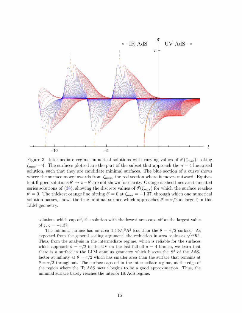
Figure 3: Intermediate regime numerical solutions with varying values of θ′(ζmax), takingζmax = 4. The surfaces plotted are the part of the subset that approach the a = 4 linearisedsolution, such that they are candidate minimal surfaces. The blue section of a curve showswhere the surface move inwards from ζmax, the red section where it moves outward. Equiva-lent flipped solutions θ′ → π−θ′ are not shown for clarity. Orange dashed lines are truncatedseries solutions of (38), showing the discrete values of θ′(ζmax) for which the surface reachesθ′ = 0. The thickest orange line hitting θ′ = 0 at ζmin = −1.37, through which one numericalsolution passes, shows the true minimal surface which approaches θ′ = π/2 at large ζ in thisLLM geometry.

solutions which cap off, the solution with the lowest area caps off at the largest valueof ζ, ζ = −1.37.

The minimal surface has an area 1.43√ε5R3 less than the θ = π/2 surface. As

expected from the general scaling argument, the reduction in area scales as√ε5R3.

Thus, from the analysis in the intermediate regime, which is reliable for the surfaceswhich approach θ = π/2 in the UV on the fast fall-off a = 4 branch, we learn thatthere is a surface in the LLM annulus geometry which bisects the S3 of the AdS5

factor at infinity at θ = π/2 which has smaller area than the surface that remains atθ = π/2 throughout. The surface caps off in the intermediate regime, at the edge ofthe region where the IR AdS metric begins to be a good approximation. Thus, theminimal surface barely reaches the interior IR AdS regime.

16

5 Discussion

We have found new examples of entanglement shadows in LLM geometries. We anal-ysed a specific example where the geometry is simple enough that we could approxi-mately determine the location of the minimal surface, but we expect this behavior tobe more general. The essential reason for the change in the minimal surface is thatthe S3 that our minimal surface divides goes from having a volume which decreasesas we moved inwards through the UV region, to being essentially constant as we enterthe IR region. When the volume of the sphere is decreasing, the minimal area surfacestretches across the ball, as in flat space. But when the volume of the sphere becomesconstant, the minimal surface wraps around the sphere at nearly constant radius, ason a cylinder. Thus we would expect that such shadows would be seen in any LLMgeometry where the volume of the S3 becomes approximately constant in the interior.That is, for cases where there are one or more white regions inside a black region.

Our story is not, however, completely generic. If we consider instead an LLMgeometry with two black discs, when the discs are well-separated we can treat theregion near each disc as an approximate copy of AdS5 × S5, and we would not expectthere to be a shadow region. There is also no reason to expect a shadow for smallfluctuations in the shape of the AdS black disc geometry.

As we vary θ0, the location of the minimal surface jumps at θ0 = π/2 from passingabove the shadow region to passing below it. However, there is an extremal non-minimal surface at θ = π/2 which passes through the shadow region. Each point inthe shadow region lies on such a surface for some choice of division of the boundary.Therefore it would be very interesting if this non-minimal surface could be interpretedin terms of a CFT observable, similar to the entwinement of [9,14]. One of the advan-tages of conducting the analysis in the LLM context is that the dual CFT states areknown precisely, so we can explore the entanglement structure of these states and see ifthey lead to interesting observables. The states correspond to Young tableaux, and itis intriguing to speculate that the SN structure encoded in these tableaux could play arole here, as the SN symmetry of the symmetric orbifold did in the entwinement story.

Another possibly related discussion is that in [24], which studies surfaces in aCoulomb branch geometry in which SU(N) is broken to SU(m)× SU(N −m) wherem,N are of similar order. They construct surfaces that bisect the S5 factor at largeradius (scales above the symmetry breaking scale) and pass between the two IR AdSfactors; whether the minimal surface in this class enters one region, the other, or nei-ther, depends on where one places the cutoff. They conjecture that surfaces passingbetween the two factors measure the entanglement between the light fields associatedwith each unbroken gauge factor.

As the cutoff is removed, all of these surfaces bisect the S5 at the equator, as provenin [23]. However, following our discussion above, none of these are minimal for anycutoff; there are always arbitrarily small extremal surfaces which only extend inwardfor a small distance away from the cutoff surface. In Figure 3 of [24], these wouldbe surfaces that pass r = 0 at larger values of y than are shown. Nonetheless, thesurfaces studied in [24] are extremal, and as with the entwinement story there maybe a plausible inerpretation in terms of entanglement explicitly involving the matrixdegrees of freedom of the theory.

17

Acknowledgements

We are grateful for useful discussions with Aitor Lewkowycz, Onkar Parrikar andCharles Rabideau. AL and AR are supported in part by DOE grant DE-SC0009987.SFR is supported in part by STFC under consolidated grant ST/L000407/1. VB wassupported by the Simons Foundation (#385592, It From Qubit Collaboration) and byDOE grant DE-FG02-05ER- 41367.

References

[1] S. Ryu and T. Takayanagi, Holographic derivation of entanglement entropy fromAdS/CFT, Phys. Rev. Lett. 96 (2006) 181602, [hep-th/0603001].

[2] V. E. Hubeny, M. Rangamani, and T. Takayanagi, A Covariant holographicentanglement entropy proposal, JHEP 07 (2007) 062, [arXiv:0705.0016].

[3] T. Faulkner, M. Guica, T. Hartman, R. C. Myers, and M. Van Raamsdonk,Gravitation from Entanglement in Holographic CFTs, JHEP 03 (2014) 051,[arXiv:1312.7856].

[4] B. Czech, L. Lamprou, S. McCandlish, B. Mosk, and J. Sully, A StereoscopicLook into the Bulk, JHEP 07 (2016) 129, [arXiv:1604.0311].

[5] J. de Boer, F. M. Haehl, M. P. Heller, and R. C. Myers, Entanglement,holography and causal diamonds, JHEP 08 (2016) 162, [arXiv:1606.0330].

[6] V. Balasubramanian, B. D. Chowdhury, B. Czech, J. de Boer, and M. P. Heller,Bulk curves from boundary data in holography, Phys. Rev. D89 (2014), no. 8086004, [arXiv:1310.4204].

[7] R. C. Myers, J. Rao, and S. Sugishita, Holographic Holes in Higher Dimensions,JHEP 06 (2014) 044, [arXiv:1403.3416].

[8] M. Headrick, R. C. Myers, and J. Wien, Holographic Holes and DifferentialEntropy, JHEP 10 (2014) 149, [arXiv:1408.4770].

[9] V. Balasubramanian, B. D. Chowdhury, B. Czech, and J. de Boer, Entwinementand the emergence of spacetime, JHEP 01 (2015) 048, [arXiv:1406.5859].

[10] B. Freivogel, R. A. Jefferson, L. Kabir, B. Mosk, and I.-S. Yang, CastingShadows on Holographic Reconstruction, Phys. Rev. D91 (2015), no. 8 086013,[arXiv:1412.5175].

[11] T. Banks, W. Fischler, S. H. Shenker, and L. Susskind, M theory as a matrixmodel: A Conjecture, Phys. Rev. D55 (1997) 5112–5128, [hep-th/9610043].

[12] V. Balasubramanian, R. Gopakumar, and F. Larsen, Gauge theory, geometryand the large N limit, Nucl. Phys. B526 (1998) 415–431, [hep-th/9712077].

[13] J. Polchinski, M theory and the light cone, Prog. Theor. Phys. Suppl. 134 (1999)158–170, [hep-th/9903165].

[14] V. Balasubramanian, A. Bernamonti, B. Craps, T. De Jonckheere, and F. Galli,Entwinement in discretely gauged theories, arXiv:1609.0399.

18

[15] J. Lin, A Toy Model of Entwinement, arXiv:1608.0204.

[16] H. Lin, O. Lunin, and J. M. Maldacena, Bubbling AdS space and 1/2 BPSgeometries, JHEP 10 (2004) 025, [hep-th/0409174].

[17] V. Balasubramanian, B. Czech, K. Larjo, and J. Simon, Integrability versusinformation loss: A Simple example, JHEP 11 (2006) 001, [hep-th/0602263].

[18] V. Balasubramanian, B. Czech, K. Larjo, D. Marolf, and J. Simon, Quantumgeometry and gravitational entropy, JHEP 12 (2007) 067, [arXiv:0705.4431].

[19] D. Berenstein and A. Miller, Superposition induced topology changes in quantumgravity, arXiv:1702.0301.

[20] D. Berenstein and A. Miller, Reconstructing spacetime from the hologram, evenin the classical limit, requires physics beyond the Planck scale, Int. J. Mod. Phys.D25 (2016), no. 12 1644012, [arXiv:1605.0528].

[21] D. Berenstein and A. Miller, Can Topology and Geometry be Measured by anOperator Measurement in Quantum Gravity?, Phys. Rev. Lett. 118 (2017),no. 26 261601, [arXiv:1605.0616].

[22] A. Mollabashi, N. Shiba, and T. Takayanagi, Entanglement between TwoInteracting CFTs and Generalized Holographic Entanglement Entropy, JHEP 04(2014) 185, [arXiv:1403.1393].

[23] C. R. Graham and A. Karch, Minimal area submanifolds in AdS x compact,JHEP 04 (2014) 168, [arXiv:1401.7692].

[24] A. Karch and C. F. Uhlemann, Holographic entanglement entropy and theinternal space, Phys. Rev. D91 (2015), no. 8 086005, [arXiv:1501.0000].

[25] J. McGreevy, L. Susskind, and N. Toumbas, Invasion of the giant gravitons fromAnti-de Sitter space, JHEP 06 (2000) 008, [hep-th/0003075].

[26] T. Nishioka and T. Takayanagi, AdS Bubbles, Entropy and Closed StringTachyons, JHEP 01 (2007) 090, [hep-th/0611035].

[27] P. A. R. Jones and M. Taylor, Entanglement entropy in top-down models, JHEP08 (2016) 158, [arXiv:1602.0482].

19