Entanglement effects in defect-free model polymer networks

OPEN ACCESS

Entanglement effects in defect-free model polymernetworksTo cite this article: Ralf Everaers 1999 New J. Phys. 1 12

View the article online for updates and enhancements.

You may also likeLong-range Rydberg–Rydberg interactionsin calcium, strontium and ytterbiumC L Vaillant, M P A Jones and R MPotvliege

-

Skyrmion clusters from Bloch lines inferromagnetic filmsDmitry A. Garanin, Eugene M.Chudnovsky and Xixiang Zhang

-

The quantum Lévy walkManuel O Cáceres and Marco Nizama

-

Recent citationsSimulation of Elastomers by Slip-SpringDissipative Particle DynamicsJurek Schneider et al

-

Elasticity of Randomly Cross-LinkedNetworks in Primitive Chain NetworkSimulationsYuichi Masubuchi

-

Effect of Chain Polydispersity on theElasticity of Disordered Polymer NetworksValerio Sorichetti et al

-

This content was downloaded from IP address 84.245.193.70 on 26/01/2022 at 10:33

https://doi.org/10.1088/1367-2630/1/1/312

https://iopscience.iop.org/article/10.1088/0953-4075/45/13/135004


https://iopscience.iop.org/article/10.1209/0295-5075/120/17005

https://iopscience.iop.org/article/10.1209/0295-5075/120/17005


https://doi.org/10.1021/acs.macromol.1c00567


https://doi.org/10.1678/rheology.49.73





Entanglement effects in defect-free modelpolymer networks

Ralf EveraersMax-Planck-Institut fur Polymerforschung, Postfach 3148, D-55021 Mainz,GermanyInstitut Curie, Section de recherche, 26 rue d’Ulm, F-75248 Paris Cedex 05,FranceInstitut fur Festkorperforschung, Forschungszentrum Julich, Postfach 1913,D-52425 Julich, GermanyE-mail: [email protected]

New Journal of Physics 1 (1999) 12.1–12.54 (http://www.njp.org/)Received 22 September 1998; online 28 July 1999

Abstract. The influence of topological constraints on the local dynamicsin crosslinked polymer melts and their contribution to the elastic propertiesof rubber elastic systems are long standing problems in statistical mechanics.Polymer networks with diamond lattice connectivity are idealized model systemswhich isolate the effect of topology conservation from other sources of quencheddisorder. By studying their behaviour in molecular dynamics simulations underelongational strain we are able to measure the microscopic deformations as wellas the purely entropic shear moduli. In our analysis we make extensive useof the microscopic structural and topological information available in computersimulations and present quantitative tests of the concepts underlying moststatistical mechanical models of rubber elasticity.

Contents

1 Introduction 3

2 Theory 112.1 The phantom model. . . . . . . . . . . . . . . . . . . . . . . . . . . . . . . . 112.2 Phantom diamond networks. . . . . . . . . . . . . . . . . . . . . . . . . . . 122.3 The constrained mode model. . . . . . . . . . . . . . . . . . . . . . . . . . . 132.4 Systems with quenched regular topology. . . . . . . . . . . . . . . . . . . . . 152.5 Classical rubber elasticity: the constrained junction models. . . . . . . . . . . 152.6 The tube model. . . . . . . . . . . . . . . . . . . . . . . . . . . . . . . . . . 16

New Journal of Physics 1 (1999) 12.1–12.54 PII: S1367-2630(99)02086-81367-2630/99/000012+54$19.50 © IOP Publishing Ltd and Deutsche Physikalische Gesellschaft

mailto:[email protected]

http://www.njp.org/

12.2

2.7 Topological theories of rubber elasticity. . . . . . . . . . . . . . . . . . . . . 17

3 The simulation model 193.1 Systems with conserved topology. . . . . . . . . . . . . . . . . . . . . . . . 193.2 Phantom chains. . . . . . . . . . . . . . . . . . . . . . . . . . . . . . . . . . 203.3 Systems with annealed topology. . . . . . . . . . . . . . . . . . . . . . . . . 203.4 Diamond networks. . . . . . . . . . . . . . . . . . . . . . . . . . . . . . . . 213.5 Regular and random inter-penetration. . . . . . . . . . . . . . . . . . . . . . 223.6 Simulation runs. . . . . . . . . . . . . . . . . . . . . . . . . . . . . . . . . . 23

4 Results 244.1 Entropic origin of the network elasticity. . . . . . . . . . . . . . . . . . . . . 244.2 Stress relaxation in deformed networks. . . . . . . . . . . . . . . . . . . . . . 244.3 End-to-end distance distributions of the network strands. . . . . . . . . . . . . 274.4 Mode analysis. . . . . . . . . . . . . . . . . . . . . . . . . . . . . . . . . . . 314.5 Entanglement analysis. . . . . . . . . . . . . . . . . . . . . . . . . . . . . . 364.6 Linking probabilities . . . . . . . . . . . . . . . . . . . . . . . . . . . . . . . 38

5 Discussion 405.1 Classical rubber elasticity. . . . . . . . . . . . . . . . . . . . . . . . . . . . . 425.2 The tube model. . . . . . . . . . . . . . . . . . . . . . . . . . . . . . . . . . 465.3 The topological approach. . . . . . . . . . . . . . . . . . . . . . . . . . . . . 475.4 Outlook . . . . . . . . . . . . . . . . . . . . . . . . . . . . . . . . . . . . . . 49

6 Summary 49

Overview

Polymer networks [1] are the basic structural element of systems as different as tire rubber andgels and have a wide range of technical and biological applications. While they have been asubject of statistical mechanics for more than sixty years, their rigorous treatment still presentsa challenge. Similar to spin glasses [3], the main difficulty is the presence of quenched disorderover which thermodynamic variables need to be averaged. In the case of polymer networks [7, 2],the vulcanization process leads not only to a randomly connected solid but freezes (due to themutual impenetrability of the polymer backbones) also the topological state of the network.While for a given connectivity the phantom model Hamiltonian for non-interacting polymerchains formally takes a simple quadratic form [4]–[6], treating the topological aspects is muchharder for several reasons: (i) Topological constraints do not enter the Hamiltonian as such,but divide phase space into accessible and inaccessible regions characterized by topologicalinvariants from mathematical knot theory [9]; (ii) The common topological invariants can beused to characterize knots formed by individual strands or links between mesh pairs. However,in principle one requires an infinte set of higher order invariants [8]; (iii) All but the most primitiveinvariants are algebraic [9] so that their statistics cannot be calculated analytically for entangledrandom walks [87].

So far no rigorous solution of the statistical mechanics of entangled polymer networks exists.Topological theories of rubber elasticity [2, 7, 8], [10]–[18] represent the most fundamental

New Journal of Physics 1 (1999) 12.1–12.54 (http://www.njp.org/)

http://www.njp.org/

12.3

approach, but encounter serious mathematical difficulties already on the level of pairwiseentanglement between meshes. Most theories do, however, omit such a detailed descriptionin favour of a mean-field ansatz where the different parts of the network are thought to move in adeformation-dependent elastic matrix which exerts restoring forces towards some rest positions.The classical theories [1, 19], [20]–[23] assume that such forces only act on the cross-linksor junction points, while the tube models [24]–[28] stress the importance of the topologicalconstraints acting along the contour of strands exceeding a minimum ‘entanglement length’.

It is the purpose of this paper to quantitatively test the ideas underlying the topological,classical and tube models in computer simulations of idealized model networks with diamondlattice connectivity. Being free of defects, these systems allow us to isolate the effects of topologyconservation from those of chemical disorder. In view of the complexity of real networks sucha simplification seems adequate and be it only in order to prepare more comprehensive studies.In particular, we address the following questions.

(i) In an attempt to give a more precise meaning to the term ‘entanglement’, what is thetopological degree of linking of the network meshes?

(ii) What is the entanglement contribution to the macroscopic shear modulus?

(iii) In what manner (i.e. classical versus tube model) do entanglements affect the microscopicmean conformations and fluctuations of the networks in the unstrained state?

(iv) How does the confinement change under strain?

(v) Is it possible to calculate the macroscopic restoring forces from the microscopicdeformations? (In particular, are there non-classical contributions to the elastic response?)

(vi) Is it possible to predict the network conformations under strain from an analysis of thefluctuations in the unstrained state (i.e. based on the knowledge of the actual strength of theconfining potentials)?

(vii) As a complementary question, can one estimate the entanglement contribution to the shearmodulus from a simple model for the topological interactions?

(viii) Is it perhaps even possible toderivethe degree of confinement or the tube model along theselines?

1. Introduction

From a macroscopic point of view, rubber-like materials have very distinct visco- andthermoelastic properties [1, 25]. They reversibly sustain elongations of up to 1000% with smallstrain elastic moduli which are four or five orders of magnitude smaller than for other solids.Maybe even more unusual are the thermoelastic properties discovered by Gough and Joule in the19th century: when heated, a piece of rubber under a constant loadcontracts, and, conversely,heat isreleasedduring stretching. With the advent of statistical mechanics it became clear thatthe stress induced by a deformation had to be almost exclusively due to adecrease in entropy.The microscopic origin of this entropy change remained, however, obscure until the discoveryof polymeric molecules and their high degree of conformational flexibility in the 1930s. Ina melt of identical chains polymers adopt random coil conformations [29] with mean-squareend-to-end distances proportional to their length,〈r2〉 ∼ N . A simple statistical mechanicalargument, which only takes the connectivity of the chains into account, then suggests that flexiblepolymers react to forces on their ends as linear,entropic springs. The spring constant,k = 3kBT

〈r2〉 ,


http://www.njp.org/

12.4

is proportional to the temperature. Treating a piece of rubber as a random network of non-interacting entropic springs (the phantom model [4]–[6], see figure1 (a) and section2.1 fordetails) qualitatively explains the observed behaviour, including—to a first approximation—theshape of the measured stress–strain curves. Within this model, the only remaining problem isthe complicated connectivity of a randomly cross- or end-linked melt of linear precursor chains.A proper treatment of the frozen chemical disorder is essential in order to understand swollennetworks [30] and the vulcanization transition [31], but seems uncritical for highly cross-linkednetworks (i.e. with many cross-links per precursor chain) [6], [32]–[34].

In this paper we are concerned with a different kind of quenched disorder which is not dueto the connectivity but another characteristic property of polymers: their mutual impenetrabilityand the resulting entanglements [1, 2, 7, 8], [10]–[28], [36]–[47]. The classical view of theentanglement problem (see figure1 and Secs.2.3and2.5 for details), often associated with thename of Flory, is to assume that the main effect is a partial suppression of the junction fluctuationsrelative to the predictions of the phantom model [19]–[23]. The oldest model of rubber elasticity,the junction affine model [1], is recovered in the limit of immobile junction points, whoseinstantaneous positions then deform affinely with the sample. The classical theories predict thatentanglements only cause a modest increase (typically up to a factor of two compared to thephantom model) of the shear modulus. In particular,G ∼ ρstrandkBT = ρ

NkBT is predicted to

vanish in the limit of infinitely long network strands.There are, however, good reasons to suspect that the classical theories overlook important

aspects of the physics of an entangled network which influence (i) the fluctuations of the networkstrandsbetweenthe junction points and (ii) the absolute value of the shear modulus. The evidencecomes from the study of non-cross-linked polymer melts, which show extremely slow relaxationas soon as the chain lengthN exceeds a phenomenological ‘entanglement length’,Ne. A simpleand very successful explanation of these effects is provided by the tube model of Edwards [24]and the reptation theory [48] of de Gennes. The idea is that the presence of the other polymersrestricts a chain to fairly small fluctuations inside a tube-like region with a cross-section of theorder of 〈r2〉 (Ne) along its coarse grained contour (figure2 (a)). A polymer can loose thememory of its initial conformation only by a one-dimensional, curvilinear diffusion along andfinally out of its original tube (‘reptation’). The geometrical constraint is relatively easy to handleanalytically and on a mean-field level the tube model provides a unified view on networks andentangled polymer melts [25]–[28]. In particular, one expects that under shear deformations eachchain segment of lengthNe behaves as an independent entropic spring, leading to a chain lengthindependent (plateau) modulusG ∼ ρ

NekBT . In a melt, this shear stress relaxes over a time

τmax ∼ N3 by reptation, while in a network the chemical cross-links suppress this mechanism.Thus, in contrast to the classical models, the tube models predict a finite shear modulus in thelimit N → ∞.

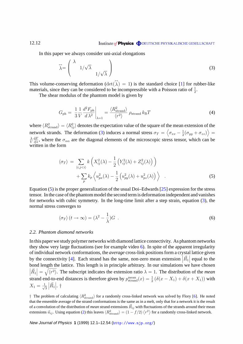
Both the constrained junction and the tube model are based on the idea that partiallyconstrained fluctuations lead to non-trivial microscopic deformations and contribute to the elasticresponse. The close relation between the two approaches (of which the tube model is in factthe older one, even though the constrained junction models completed the classical theories) isemphasized in two recent models by Rubinstein and Panyukov [41] and the present author [42].For quantitative comparisons we use in this paper the constrained mode model (CMM) [42](section2.3) which is particularly suited for the analysis of simulation data. The CMM is basedon the assumption that deformation dependent linear forces couple to (approximate)eigenmodesof the phantom network. On the one hand (figure1), we use Einstein modes describing the


http://www.njp.org/

12.5

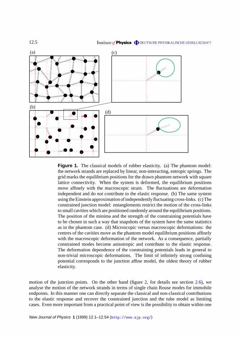
(a)

(b)

(c)

(d)

Figure 1. The classical models of rubber elasticity. (a) The phantom model:the network strands are replaced by linear, non-interacting, entropic springs. Thegrid marks the equilibrium positions for the drawn phantom network with squarelattice connectivity. When the system is deformed, the equilibrium positionsmove affinely with the macroscopic strain. The fluctuations are deformationindependent and donot contribute to the elastic response. (b) The same systemusing the Einstein approximation of independently fluctuating cross-links. (c) Theconstrained junction model: entanglements restrict the motion of the cross-linksto small cavities which are positioned randomly around the equilibrium positions.The position of the minima and the strength of the constraining potentials haveto be chosen in such a way that snapshots of the system have the same statisticsas in the phantom case. (d) Microscopic versus macroscopic deformations: thecentres of the cavities move as the phantom model equilibrium positions affinelywith the macroscopic deformation of the network. As a consequence, partiallyconstrained modes become anisotropic and contribute to the elastic response.The deformation dependence of the constraining potentials leads in general tonon-trivial microscopic deformations. The limit of infinitely strong confiningpotential corresponds to the junction affine model, the oldest theory of rubberelasticity.

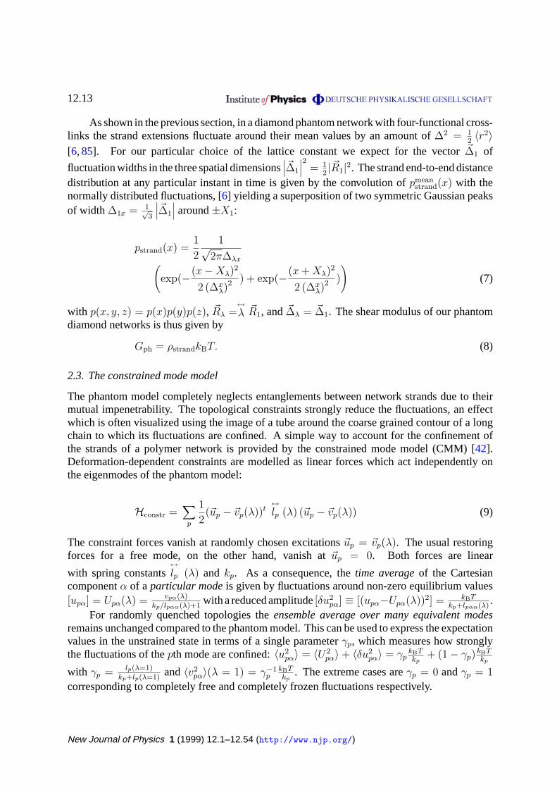
motion of the junction points. On the other hand (figure2, for details see section2.6), weanalyse the motion of the network strands in terms of single chain Rouse modes for immobileendpoints. In this manner one can directly separate the classical and non-classical contributionsto the elastic response and recover the constrained junction and the tube model as limitingcases. Even more important from a practical point of view is the possibility to obtain within one


http://www.njp.org/

12.6

(a)

(b)

(c)

(d)

(e)

Figure 2. The tube model: (a) Entanglements confine a network strand withNstrand > Ne to a tube-like region around its coarse-grained contour. (b) Theconformation of the strand can be written as a superposition of independentRouse modes for fixed endpoints. The dotted lines and shaded areas indicatethe larger range of thermal excitation of long (blue) than short (red) wavelengthmodes. (c) The constrained mode model: entanglements are modeled as actingindependently on each Rouse mode. Short wave length modes are not affectedby the tube-like constraint, while long wave length modes are restricted tofluctuations around a non-vanishing mean value which are much smaller thantheir thermal fluctuations. The formal treatment is identical for the Rouse andthe Einstein modes in figure1 (d) (e) In particular, as the tube deforms withthe sample, partially constrained modes become anisotropic and contribute tothe restoring forces. The deformation-dependence of the constraining potentialsleads to weaker than affine microscopic deformations.

transparent formalism meaningful results for systems with arbitrary strand lengthsN , rangingfrom networks withN Ne, which should be well described by classical rubber elasticity, toentanglement dominated systems withN Ne.

Topological theories of rubber elasticity have an even longer history than the tube model andrepresent a more fundamental approach, from which it might be possible toderivethe constrainedfluctuation models (including estimates for the parameters characterizing thestrengthof theconfinement such as the entanglement lengthNe). Thirty years ago, Prager and Frisch [10],Edwards [7], and later Vologodskiiet al [37, 38] argued that forces can be transmitted betweentwo ring polymers which are not chemically connected but topologically linked. Edwards [2, 7, 8]suggested calculating the elastic response from quenched averages in which topological invariantscharacterizing the degree of linking of all mesh pairs are conserved. This represents already


http://www.njp.org/

12.7

(a)

(c1)

>>> <<<

<<< >>><<< >>>

>>> <<<<<< >>>

<<< >>>(b)

(c2) (c3)

(d1)

(d2)

I=-1 I=-1 I=0

I=3

Figure 3. The topological models of rubber elasticity: (a) The topological stateof a network is a conserved quantity. Often one considers only the pairwiseentanglement of the network meshes, even though in principle an infinite set ofhigher order interactions should be taken into account as well. (b) Example oftwo multiply entangled meshes in random IPDN withN = 44. (c) The Gausslinking number,I, is a simple topological invariant. It can either be calculatedfrom a double integral over the ring contours (Eq.19) or by a method whereall crossing points of the two curves in a projection are indexed by±1/2 [35].The sign depends on the direction into which the tangent vector of the uppercurve has to be rotated in order to coincide with the one of the bridged curve.The linking numberI is defined as the sum of the indices and isinvariant underdistorsions of the rings (c2). There are examples of linked curves withI = 0,so that the classification is not completely reliable (c3). (d1) Approximation ofthe topological pair interaction by an entropic attraction (respectively repulsion)between the centres of mass (CM) of topologically linked (respectively non-linked) meshes. The origin of this effect lies in the reduction of the number ofaccessible states for two linked ring polymers with increasing CM distance. Theprecise form of the effective potential follows from the CM distance dependentlinking probability. (d2) In a simple application of these ideas to networks onecan estimate a link contribution to the shear modulus from the assumption thatthe mesh centres move affinely with the macroscopic deformation and that theeffective topological interaction is deformation independent.

a drastic simplification as in principle an infinite set of topological invariants is required tocharacterize the state of a network [8]. So far even the binary entanglement problem has proventoo complex for a rigorous solution [2],[12]–[18], but the underlying physics is preserved in the


http://www.njp.org/

12.8

simple model by Graessley and Pearson [11] (figure3, for details see section2.7). In particular,its predictions for the entanglement contribution to the shear modulus can be tested quantitativelyin computer simulations [49]. Here we will provide more details, but note already at this pointthat even though the results are encouraging for the present systems, a different approach willbe required in order to actually derive the tube model [15, 50].

Not least due to their technical importance, rheological studies on polymer networks havebeen an area of active research for more than half a century. It is therefore quite remarkable thatthere is no definite experimental answer to the question, if and how much entanglement effectscontribute to the elasticity of such systems [51]–[64]. Most of the experimental data seems to bewell described by the classical models. The constrained junction models [19]–[23] in particularhave been shown to provide an excellent parametrization of the stress–strain curves [58, 63].However, often the data can be described equally well by expressions derived from tube modelsor variants thereof [55]–[57], [65]. In fact, it is even possible to derive formally identical stress–strain relations from models which have completely opposite views on the effect of topologicalconstraints [66]. The distinction between the various theoretical approaches can therefore notbe made on the basis of theshapeof stress–strain curves alone.

A critical test requires a comparison of the absolute values of measured and predictedmoduli or, less specifically, the extrapolation of the measured moduli to the limit of vanishingcross-link density where the classical contribution to the modulus vanishes. Such investigationshave indicated from early on that the classical theories underestimate the modulus [51, 52].However, it is quite difficult to prepare model networks with a well defined density of chains inthe elastically active cluster,ρstrand. This holds in particular in the limitN Ne. A randomlycross-linked melt of linear polymers has a highly irregular connectivity. Typical defects arepolydispersity, dangling ends and clusters, and self-loops. Efforts have therefore concentratedon the preparation of model networks by end-linking. While some groups have claimed tohave prepared nearly ideal networks [58]–[60], others have shown that this state is impossibleto reach for large strand lengths [53, 54]. The reason for the imperfect network structures arethe exponentially long times required towards the end of the synthesis to pair the remainingunsaturated chain ends [67]. Patelet al [62] have used swelling experiments in order to restricttheir analysis to those of their samples with the highest degree of conversion. Their resultsindicate indeed a non-vanishing shear modulus in the limit of infinite strand length.

A more detailed test and comparison of the theoretical models requires access to microscopicinformation not available in rheological experiments. Much insight can be gained experimentallyin small-angle neutron-scattering experiments [68]–[70]. By these techniques it is, for example,possible to detect and quantify the tube-like confinement of the chain motion in polymer meltsand networks, to investigate the effect of shear deformations on the tube, and to compare theresults to theoretical predictions.

An alternative, which we shall pursue in this paper, are large scale computer simulations ofsuitably coarse-grained polymer models [71]. Bearing in mind the limitations in the accessibletime and length scales, they offer a couple of advantages compared to experiments: a greaterfreedom in and control over the formation of the networks, a more direct access to the microscopicstructure and dynamics (e.g. the restriction of the data analysis to elastically active chains),and the realization of Gedankenexperiments such as the comparison of otherwise identicalsystems with and without topology conservation. Simulations of coarse-grained models providedthe first direct evidence for the tube/reptation model in polymer melts [72, 73], gave insideinto the kinetics of end-linking [67, 74] and the structure of the resulting networks [75],


http://www.njp.org/

12.9

demonstrated the importance of topological constraints for the relaxation of cross- and end-linked networks [75, 76], and showed quantitatively the failing of the predictions of the classicalmodels for the elastic modulus [77, 78]. An important point is the good agreement betweenexperimental and simulation results for the chain mobilities and the elastic properties whenmapped onto universal curves [71] as it confirms that the simulation methods we employ arecapable of covering the experimentally relevant time and length scales.

In this paper we give a detailed account of molecular dynamics simulations of modelpolymer networks with diamond lattice connectivity [49], [78]–[80]. While such systemscannot be prepared experimentally, they offer some considerable advantages in a numericalstudy addressing fundamental aspects of the entanglement problem. First, since there are no‘chemical’ defects, diamond networks isolate the effects of topology conservation from thoseof other types of quenched disorder. Second, in the absence of dangling ends and clusters, thelongest relaxation times in these systems are the Rouse times of single network strands.

The individual diamond networks are spanned across the simulation volume via periodicboundary conditions. In the spirit of the Flory-Rehner four-chain model [81] we have chosenan average distance between connected cross-links equal to the root mean square end–to–enddistance of the corresponding chains in a melt. The density of a single diamond net decreaseswith the strand length. To reach melt density we place several of these structures in the simulationbox and work with inter-penetrating diamond networks (IPDN). As a consequence, cross-linkswhich are nearest neighbours in space will usually belong to different diamond nets and will notbe connected by network strands. The same holds true in experimental systems, which can besaid to belocally inter-penetrating [20]. The regular connectivity in our systems affects onlylength scales beyond the size of the network strands.

We follow two distinct strategies to isolate the entanglement effects. One is to calculatequenched averages for otherwise identical systems with different topology. In our simulationsof random and of regular IPDN we employ interaction potentials which ensure the mutualimpenetrability of the chains, thereby preserving the topological state from the end of thepreparation process. The second strategy is to calculate annealed averages over differenttopologies. This can either be achieved trivially by simulating non-interacting phantom chainsor by using interaction potentials that allow chains to cut through each other but neverthelesspreserve the monomer packing of the melt [76]. The structure of the chains is almost identical forall systems and by comparing their behaviour we can directly access the effects of the topologicalconstraints. The preparation of our most important systems, the random IPDN, is illustrated invideo-sequence 1.

By investigating strained samples we obtained the first reliable measurements of the elasticproperties of model polymer networks in a computer simulation [78, 79]. Since we also havecomplete access to the microscopic structure and dynamics in both, the strained and the unstrainedstate, we are in a unique position to test statistical mechanical theories of rubber elasticity whichare based on a well-defined microscopic picture. While the quantitative analysis will exclusivelybe concerned with moderate deformations of the order of 50%, some qualitative insight intothe importance of entanglements can already be gained by analysing the microscopic stressdistribution in strongly stretched random IPDNs as in figure4and the video sequence 2. Chemicalbonds which carry high tensions are shown with a larger diameter and marked in red. A large partof the tension is localized on topologically shortest paths through the system. In particular, thesepaths are composed of strands as well as meshes with physical entanglements propagating thetensionin the same manner as chemical cross-links. This stress localization in random IPDNs is


http://www.njp.org/

12.10

Figure 4. Conformation of highly strained random IPDN (λ = 3.2) [80]. In thenon-linear regime a large part of the stress is localized on topologically shortestpaths through the system (bonds carrying high tensions are marked by thick radiiand in red). Note that physical entanglements propagate the tension in the samemanner as chemical cross-links. The apparant interruption of the chains is due tothe representation in periodic boundary conditions.

completely unexpected from the point of view of the classical theory, since all network strandsare equivalent. The more artificial regularly IPDN mimic a situation where this equivalence ispreserved for a conserved topology. When these networks are stretched, all strands contributeequally to the elastic response. Tensions are homogeneous throughout the whole system, and allstrands are stretched to their full contour length at the maximal elongation.

In order to keep the paper in spite of its considerable length accessible to the reader, wehave tried to structure the presented material as much as possible. For a first reading, it should bepossible to pass directly to the discussion in section5. The theoretical background is presentedin section2, a description of the simulation techniques and the detailed presentation of thesimulation results can be found in sections3 and4 respectively. Two key results of this studyhave already been published in short notes: the direct proof that the classical explanation ofrubber elasticity which only considers the elongation of the network strands cannot accountfor the observed moduli [78] and the interpretation of the topology contribution to the elasticmodulus in terms of mesh entanglements [49]. The graphical illustrations of the preparation ofrandom IPDN and their behaviour under large strain (including a visualization of the propagationof internal stresses by entanglements) were first published in [80]. Some preliminary results haverecently been presented at the 11th Max-Born conference [82].


http://www.njp.org/

12.11

2. Theory

Most current models of rubber elasticity are based on the phantom model [4]–[6] (section2.1)combined with the idea that entanglements between the polymer chains reduce thefluctuations [1], [25]–[28]. Being deformation dependent, the effective constraints thencontribute to the elastic properties of the network. In section2.3 we discuss these effectsin the framework of the constrained mode model (CMM) [42]. The results are then used insections2.5 and2.6 to recover the classical theories of rubber elasticity and the tube model.Finally, we present in section2.7 the simple topological model of Graessley and Pearson [11].Secs.2.2 and 2.4 discuss phantom diamond networks and systems with a quenched regulartopology.

2.1. The phantom model

The Hamiltonian of the phantom model [4]–[6] is given byHph = k2∑

〈i,j<i〉 r2ij, where〈i, j < i〉

denotes a pair of nodes which are connected by a polymer chain acting as an entropic spring ofstrengthk = 3kBT

〈r2〉 and~rij(t) = ~ri(t) − ~rj(t) the distance between them. The problem is mostconveniently studied using periodic boundary conditions, which span the network over a fixedvolume [2].

Due to the linearity of the springs the problem separates in Cartesian co-ordinatesx, y, z.Furthermore, a conformation of a network of harmonic springs can be analysed in terms of eitherthe bead positions~ri(t) or the deviations~ui(t) of the nodes from their equilibrium positions~Ri.The latter are characterized by a force equilibrium

∑j

~Rij ≡ 0, wherej indexes all nodes whichare connected with nodei. In this representation, the Hamiltonian separates into two independentcontributions from the equilibrium extensions of the springs and the fluctuations, which can bewritten as a sum over independent normal modes or phonons~up [83, 84]:

Hph =k

2∑

〈i,j<i〉~R2

ij +kp

2∑p

~u2p (1)

If a sample is deformed, the equilibrium positions of the junction points change affinely. Thefluctuations, on the other hand, depend only on the connectivity but not on size and shape ofthe network. The shear modulus of the phantom model can therefore be calculated withouthaving to integrate out the dynamic eigenmodes of the network. Structural averages, on theother hand, do depend on the fluctuations. Consider, for example, the mean-square extension~R2

ij + [~u2ij] of a network strand.† It follows from the equipartition theorem that the total thermal

energy in the fluctuations,Ufluc, is given by 32kBT times the number of modes and therefore

Ufluc = 32kBTNnodes = 2

f32kBTNstrands, whereNnodes andNstrands are the number of junction

points and network strands, which are related byNstrands = f2Nnodes in anf -functional network.

Equating the thermal energy per strand tok2

⟨~u2

ij

⟩, one obtains [6, 42, 85]

〈u2ij〉 =

2f

⟨r2⟩

. (2)

† We use[. . .] to denote time and〈. . .〉 to denote ensemble averages.


http://www.njp.org/

12.12

In this paper we always consider uni-axial elongations

↔λ=

λ

1/√

λ

1/√

λ

(3)

This volume-conserving deformation (det(↔λ) = 1) is the standard choice [1] for rubber-like

materials, since they can be considered to be incompressible with a Poisson ratio of12 .

The shear modulus of the phantom model is given by

Gph =13

1V

d2Fph

d λ2

∣∣∣∣∣λ=1

=〈R2

strand〉〈r2〉 ρstrand kBT (4)

where〈R2strand〉 = 〈R2

ij〉 denotes the expectation value of the square of the mean extension of the

network strands. The deformation (3) induces a normal stressσT =⟨σxx − 1

2(σyy + σzz)⟩

=λV

dFdλ

, where theσαα are the diagonal elements of the microscopic stress tensor, which can bewritten in the form

〈σT 〉 =∑

〈i,j<i〉k(X2

ij(λ) − 12

(Y 2

ij(λ) + Z2ij(λ)

) )

+∑p

kp

⟨u2

px(λ) − 12

(u2

py(λ) + u2pz(λ)

)⟩. (5)

Equation (5) is the proper generalization of the usual Doi–Edwards [25] expression for the stresstensor. In the case of the phantom model the second term is deformation independent and vanishesfor networks with cubic symmetry. In the long-time limit after a step strain, equation (3), thenormal stress converges to

〈σT 〉 (t → ∞) = (λ2 − 1λ

)G . (6)

2.2. Phantom diamond networks

In this paper we study polymer networks with diamond lattice connectivity. As phantom networksthey show very large fluctuations (see for example video6). In spite of the apparent irregularityof individual network conformations, theaveragecross-link positions form a crystal lattice givenby the connectivity [4]. Each strand has the same, non-zero mean extension

∣∣∣~R1

∣∣∣ equal to thebond length the lattice. This length is in principle arbitrary. In our simulations we have chosen∣∣∣~R1

∣∣∣ =√

〈r2〉. The subscript indicates the extension ratioλ = 1. The distribution of themean

strand end-to-end distances is therefore given bypmeanstrand(x) = 1

2 (δ(x − X1) + δ(x + X1)) with

X1 = 1√3

∣∣∣~R1

∣∣∣. †† The problem of calculating〈R2

strand〉 for a randomly cross-linked network was solved by Flory [6]. He notedthat the ensemble average of the strand conformations is the same as in a melt, only that for a network it is the resultof a convolution of the distribution ofmeanstrand extensions~Rij with fluctuations of the strands around their meanextensions~uij . Using equation (2) this leaves〈R2

strand〉 = (1 − f/2)⟨r2⟩

for a randomly cross-linked network.


http://www.njp.org/

12.13

As shown in the previous section, in a diamond phantom network with four-functional cross-links the strand extensions fluctuate around their mean values by an amount of∆2 = 1

2 〈r2〉[6, 85]. For our particular choice of the lattice constant we expect for the vector~∆1 of

fluctuation widths in the three spatial dimensions∣∣∣~∆1

∣∣∣2 = 12 |~R1|2. The strand end-to-end distance

distribution at any particular instant in time is given by the convolution ofpmeanstrand(x) with the

normally distributed fluctuations, [6] yielding a superposition of two symmetric Gaussian peaksof width ∆1x = 1√

3

∣∣∣~∆1

∣∣∣ around±X1:

pstrand(x) =12

1√2π∆λx(

exp(−(x − Xλ)2

2 (∆xλ)

2 ) + exp(−(x + Xλ)2

2 (∆xλ)

2 ))

(7)

with p(x, y, z) = p(x)p(y)p(z), ~Rλ =↔λ ~R1, and~∆λ = ~∆1. The shear modulus of our phantom

diamond networks is thus given by

Gph = ρstrandkBT. (8)

2.3. The constrained mode model

The phantom model completely neglects entanglements between network strands due to theirmutual impenetrability. The topological constraints strongly reduce the fluctuations, an effectwhich is often visualized using the image of a tube around the coarse grained contour of a longchain to which its fluctuations are confined. A simple way to account for the confinement ofthe strands of a polymer network is provided by the constrained mode model (CMM) [42].Deformation-dependent constraints are modelled as linear forces which act independently onthe eigenmodes of the phantom model:

Hconstr =∑p

12(~up − ~vp(λ))t

↔lp (λ) (~up − ~vp(λ)) (9)

The constraint forces vanish at randomly chosen excitations~up = ~vp(λ). The usual restoringforces for a free mode, on the other hand, vanish at~up = 0. Both forces are linear

with spring constants↔lp (λ) and kp. As a consequence, thetime averageof the Cartesian

componentα of a particular modeis given by fluctuations around non-zero equilibrium values[upα] = Upα(λ) = vpα(λ)

kp/lpαα(λ)+1 with a reduced amplitude[δu2pα] ≡ [(upα−Upα(λ))2] = kBT

kp+lpαα(λ) .For randomly quenched topologies theensemble average over many equivalent modes

remains unchanged compared to the phantom model. This can be used to express the expectationvalues in the unstrained state in terms of a single parameterγp, which measures how stronglythe fluctuations of thepth mode are confined:〈u2

pα〉 = 〈U2pα〉 + 〈δu2

pα〉 = γpkBTkp

+ (1 − γp)kBTkp

with γp = lp(λ=1)kp+lp(λ=1) and〈v2

pα〉(λ = 1) = γ−1p

kBTkp

. The extreme cases areγp = 0 andγp = 1corresponding to completely free and completely frozen fluctuations respectively.


http://www.njp.org/

12.14

With the choice [42] ~vp(λ) =↔λ ~vp and

↔lp (λ) =

(↔λ

)−2 ↔lp of affinely moving and deforming

constraints the model is now completely specified and some general conclusions can be drawnwith respect to the microscopic deformations. The mean excitations,

Upα(λ)Upα(1)

=λαα

(1 − γp)λ2αα + γp

, (10)

of partially frozen modes deformsub-affinely. Only in the limitγp → 1 one findsUp(λ) =λUp(1). A similar result holds for the width of the fluctuations:

〈δu2pα(λ)〉

〈δu2pα(1)〉 =

λ2αα

(1 − γ)λ2αα + γ

. (11)

While the fluctuations are deformation-independent for unconstrained modes, their widthincreases sub-affinely for0 < γ < 1. For completely frozen modes withγ ≡ 1, 〈δu2

pα(λ)〉 ≡ 0independent ofλ. Not surprisingly, the predictions concerning the elastic properties are alsomodified compared to the phantom model. First, the confined fluctuations contribute to thesmall-strain shear modulus:

Gcm = Gph +kBT

V

∑p

γ2p . (12)

Second, they produce corrections to the ideal stress–strain behaviour equation (6), which isrecovered only in the two limiting cases ofγ = 0 and γ = 1. When plotted in the usualMooney–Rivlin form [42], the corrections qualitatively resemble those observed in experiments,which is encouraging but certainly no proof for the correctness of the ansatz.

An interesting point for the data analysis is the continued validity [42] of equation (5)within the CMM (or any other model with affinely deforming constraints) even for partiallyconfined modes. While the true and the entropic normal tensions can therefore be directlycompared, this is not the case for the elastic free energy, which is partially stored in theconstraints. The time evolution and confinement of the different modes is best characterized bythe ensemble average of their auto-correlation functioncp(t) = 〈~up(t) · ~up(0)〉. The quantitiesdiscussed in the CMM are related to this function by:〈u2

p〉 = cp(0), 〈U2p 〉 = limt→∞ cp(t), and

〈δu2p〉 = limt→∞(cp(0) − cp(t)). The auto-correlation functions can also be used for a heuristic

generalization of equation (12) to a time-dependent shear relaxation modulus

Gcm(t) = Gph +kBT

V

∑p

〈~up(t) · ~up(0)〉⟨~u2

p

⟩2

. (13)

Equation (13) reduces to the Rouse-model result [25] GRouse(t) = Gph + kBTV

∑p e−2t/τp for

γ = 0 and should decay to the asymptotic value (12) on similar time scales as the true shearrelaxation modulus. Equation (13) is slightly different from the expression employed by Dueringet al [72, 75, 77]. For a discussion of this point see [42].


http://www.njp.org/

12.15

2.4. Systems with quenched regular topology

A particular situation arises in systems with a conservedregular topology such as our regularIPDN. In this case, the fluctuations~δup are reduced compared to the phantom model but, due tosymmetry, for each mode centred around zero. For the same reason, the time average for eachindividual mode is identical to the ensemble average over all equivalent modes. However, thelatter now differs from the phantom network value. Within the above model,~vp(λ) = ~Up(λ) = 0and〈δu2

pα〉 = (1 − γpα)〈u2pα〉ph, whereγ is defined as before. The deformation dependence

is now exclusively described by equation (11). Quite interestingly, there is a contribution tothe shear modulus of the formGcm = Gph + kBT

V

∑p γp(1 − γp) even though the mode auto-

correlation functions decay to zero. In contrast to the random case, a completely confined modehas a (deformation independent) zero excitation and does therefore not contribute to the shearmodulus. For asymmetric confinement,γp|| 6= γp⊥, there is a non-vanishing normal stress atzero strain and it is no longer possible to define a simple shear modulus.

2.5. Classical rubber elasticity: the constrained junction models

The classical theories of rubber elasticity [1], [4]–[6], [19]–[23] date back more than half acentury and can qualitatively explain many aspects of the physics of rubber elasticity. They arebased on the assumption that the elastic response of rubber has its sole origin in the elongationof the network strands. In this view the main effect of entanglements is a partial suppression ofthe junction fluctuations [19]–[23]. The latter are usually treated as independent, i.e. using theEinstein model for phonons. The parameterγp corresponds toγ = κ

κ+1 in Flory’s first paper onconstrained junction models [20].

Consider a particular junction pointi of anf -functional network. If one assumes that itstopological neighbours are fixed at their equilibrium positions~Rj, a displacementuiα of nodei

in one spatial directionα requires an energyfk2 u2

iα. Treating these displacements as independenteigenmodes (‘Einstein modes’) with spring constantkp = fk, one can use the equipartitiontheorem to obtain〈u2

iα〉 = kBTfk

. As a consistency check, we note that this result implies thatthe extension of a particular network strand should undergo thermal fluctuations of a width〈|~uij|2〉 = 2〈|~ui|2〉 = 2 × 3kBT

fk= 2

f〈r2〉 in agreement with equation (2). In fact, using this

argument one can simplify the data analysis and follow the fluctuations of the extensions of thenetwork strands instead of the cross-link motion.

The strength of the confinement can be estimated using arguments from the tube model.For network strands whose length exceed the melt entanglement lengthNe the fluctuationsof the junction points are restricted to the tube diameter〈r2〉 (Ne). In this case one findsNe ∼ 〈δu2

pα〉 = (1 − γp)〈u2pα〉 ∼ (1 − γp)N or γ = 1 − Ne

N. Contrary to what one might

expect, the constrained junction model predicts deformations of the mean strand extensions,which forλ >

√N/Ne are much weaker than affine. This was already noted by Flory, who did,

however, not make the connection to the tube model.In the limit of infinitely long chains,N → ∞, one recovers the predictions of the oldest

model of rubber elasticity, the junction affine model. Using the result that there are2f

modes pernetwork strand and equation (8) for the shear modulus of the phantom model the CMM predicts:

Gaff =32ρstrandkBT (14)


http://www.njp.org/

12.16

The junction affine model assumes that the surrounding molecules suppress the movements ofthe junction points so strongly that the latter’s instantaneous positions (and not only their meanpositions as in the case of the phantom model) change affinely with the shape of the sample. For

the diamond networks this implies~Rλ =↔λ ~R1 and~∆λ =

↔λ ~∆1 and leads directly to equation (14).

Note, that the affine model constitutes anupper limitfor the modulus predicted from a classicaltheory.† In a first test [78] of the classical picture we have shown that the shear moduli ofrandom IPDN exceed the affine limit, providing quantitative proof that one cannot calculate theelastic moduli from this ansatz. In this paper we present a more detailed comparison betweenour simulation results and the predictions of the constrained junction models.

2.6. The tube model

At present, the tube model of Edwards [24] and the reptation theory of de Gennes [48] are the mostsuccessful approach to the problem of entangled polymer systems [25]–[28]. The geometricalconstraint is much easier to handle than the topological constraints discussed in the followingsection.

In section2.1we have discussed phantom networks where the strands between the(f > 2)-functional junction points are replaced by a entropic spring of strengthk. In addition to theconstraints on the motion of the junction points introduced in the previous section, the non-classical theories of rubber elasticity consider restrictions of the fluctuations of the strandsbetween the junction pointssuch as tubes or slip-links [11, 43]. It is easy to see that dividing thenetwork strands into Gaussian sub-strands (i.e. formally introducing additional, two-functionaljunction points along the strands) changes nothing for a phantom network. The spring constantis doubled for a strand of half the original length, i.e. if an entropic spring of spring constantk is replaced by a linear sequence ofN springs the latter have a spring constant ofN k.Furthermore, the equilibrium positions of the new (f = 2) functional cross-links are alongthe line connecting the equilibrium positions of the original endpoints. Since〈R2

N〉 = 1N2 〈R2〉,

one findsk N∑N

i=1〈R2N〉 = k〈R2〉 and the predicted modulus remains unchanged.†

The fluctuations of the strand conformations between the cross-links are most naturallyanalysed in terms of single chain Rouse-modes [25]. Duering et al [72, 75] have used thismethod to characterize the relaxation of entangled chains in (un)cross-linked melts [72, 75].For the present purposes, it turns out to be convenient to regard the chain ends as fixedat ~r0(t) ≡ ~R0 and~rNstrand(t) ≡ ~RNstrand in contrast to the previously used open boundaryconditions [72, 75]. One can then expand the deviations~ui(t) = ~ri(t)− ~Ri from the equilibriumpositions~Ri = ~R0 + i/Nstrand

(~RNstrand − ~R0

)in terms of sin-Rouse-modes:

~up(t) =1

Nstrand + 1

Nstrand∑i=0

~ui(t) sin(

pπi

Nstrand

)(15)

† The ratioGaff/Gph = 3/2 is an artifact of our choice of⟨r2⟩1/2

for the bond length of the diamond lattice. In

general, for anf -functional lattice one recovers the standard relationGaff/Gph = ff−2 by setting~R 2

1 = f−2f

⟨r2⟩.

† Gao and Weiner [86] recently analysed the stress relaxation in a sheared melt of long-chain molecules alongthese lines from a sub-strand analysis. For many purposes this method is equivalent to the mode analysis. Thelatter offers the advantage of being compatible with the CMM and of naturally providing the length scales whereentanglement effects become relevant.


http://www.njp.org/

12.17

H =k

2

(~R0 − ~RNstrand

)2+∑p

kp

2~u2

p (16)

kp =2π2k

Nstrandp2 (17)

As the Einstein modes describe the fluctuations of thejunction points, the Rouse modes (15)describe the fluctuations of themonomersaround their respective equilibrium positions. Togetherthe Einstein and the Rouse modes form a complete and orthogonal basis set. In particular, theyare like the true eigenmodes of the phantom modelindependentof size and shape of the networkand allow a simple distinction between classical and non-classical entanglement effects.

We can again use the CMM to discuss the consequences of a confinement of the Rousemodes due to entanglements. Consider the limit of long strands ofNstrand → ∞ Gaussianunits, where the classical contribution to the shear modulus becomes negligible:Gclass ≤ Gaff =

ρNstrand

kBT → 0 (ρ here denotes the number density of the Gaussian units). The simplest ansatz

for thep-dependence of the confinement parameter is a step functionγp = Θ(p − Nstrand

Ne

), so

that all modes with a wavelength larger than the entanglement length,Ne, are completely frozen.The shear modulus is obtained by multiplying the number of frozen modes per chain,Nstrand/Ne,with the chain densityρ/Nstrand:

Gtube =Nstrand

Ne

ρ

NstrandkBT =

ρ

NekBT. (18)

As already discussed in section2.3, partially frozen modes with0 < γp < 1 lead to a weakerthan affine deformations of both, the tube axes and the tube diameter, and to the characteristicMooney–Rivlin corrections to the ideal stress–strain curves.

2.7. Topological theories of rubber elasticity

Already thirty years ago Edwards had outlined the two essential steps in a rigorous treatmentof the topological constraints [7, 8]. The first step is the characterization of the state of thenetwork in terms of an—in principle infinite—set of topological invariants. For example, theGauss linking number (GLN)

I =14π

∮ ∮ (d~r1 × d~r2) · (~r1 − ~r2)|~r1 − ~r2|3 = 0, ±1, . . . (19)

could be used to distinguish between entangled (I 6= 0) and non-entangled pairs of loops ormeshes [87]. Although the use of the GLN is only justified for simple link topologies [87], it is theonly topological invariant which can be incorporated into the standard polymer formalism [2, 87]

The second step is the calculation of the elastic response from quenched averages in whichthese invariants are conserved. Analytic attempts along these lines are very complex [2, 12, 13]even though they only take two-loop interactions into account. They require numerous andoften uncontrolled approximations and no satisfactory treatment has been put forward so far.A principal problem in the development of topological theories is the question how they canbe tested experimentally. At least to our knowledge, there is no experimental technique thatcould provide information on the microscopic topological state of a sample and thus help to testthe validity of the underlying concepts. Computer simulations offer the unique possibility toovercome this difficulty. In fact, we chose the particular geometry of the IPDN with the intention


http://www.njp.org/

12.18

to determine the linking states of the meshes of these conveniently regular networks. Our analysisis based on [49] a theory which is complementary to the single-chain ansatz described above.The model of Graessley and Pearson [11] defines entanglements as links between closed loops(meshes) of the network. Their effects are included as additional entropic springs acting betweenthe mesh centres of mass (CM). The effects on the strand conformations are ignored.

The underlying idea of an entropic interaction between two loops due to the conservation oftheir topological state was introduced by Vologodskiiet al [37, 38]. Consider two rings of lengthN with CM distance~r. If the rings do not interact, then for all values of~r the accessible phasespace volumeΩ is trivially given by the product of the phase space volumes of the individualrings. Naturally, there is no restoring force if the distance of the rings changes. The situation isdifferent if topology conservation is introduced. The phase space becomes divided into disjunctregions for topologically equivalent conformations. To a first approximation, there are onlytwo classes, linked and non-linked rings, so thatΩlinked(~r) + Ωnon−linked(~r) = Ω. Consider theentropy of an ensemble of ring pairs which had a CM distance~r0 when the topology conservationwas introduced†. The probability that the rings are linked is given byf(~r0) = Ωlinked(~r0)/Ω.The entropy of the ensemble,S = f(~r0)kB log(f(~r)) + (1 − f(~r0))kB log(1 − f(~r)), thus notonly depends on the actual ring distance~r but also on~r0. In fact, for small deviations from theoriginal distance one can writeS(~r) = S(~r0)− f ′2(~r0)

f(~r0)(1−f(~r0))(r − r0)2. While the individual ringpairs either attract or repel each other depending on whether or not they are linked, there isonaveragea (linear) restoring force to the state the members of the ensemble were in, when thetopology was quenched.

For the chain length dependence of the linking probability one expectsfN(r) = f(r/N1/2),even thoughf(~x) is not generally known. There are some rigorous results [88], approximativeanalytic treatments [89]–[91], [17], Monte Carlo simulations of pairs of closed random walks ona lattice [37, 38, 50, 88, 92], and our own results for the meshes of the diamond networks [49].For finite N it turns out to be useful to define a ‘linking radius’4π

3 R3L = 1

2

∫d3r fN(~r) and

to considerfN(r) = f(r/RL(N)) in order to reduce the finite size corrections to the scaleddistribution function.

For loops which are randomly distributed in space with a densityρloop and a sphericallysymmetric linking probability one can define an entanglement (link) density:

ρlink = 2πρ2loopR

3L

∫ ∞

0x2 f(x) dx . (20)

In their attempt to estimate the topology contribution to the shear modulus of polymer networksGraessley and Pearson (GP) [11] assumed (1) thatf(~x) remains unchanged under deformationsof the sample, i.e. they ignored distortions of the loop shapes, (2) that the contributions of thedifferent loop pairs are independent and additive, and (3) that the positions of the loop CM

change affinely with the deformation↔λ of the sample. The loop contributionGlink to the shear

modulus can be written in the form:

Glink = a[f(x)] ρlink (21)

a[f(x)] =kBT

15

∫∞0

x4f ′2(x)f(x)(1−f(x)) dx∫∞

0 x2 f(x) dx. (22)

† In an experiment this is the moment when the second ring is closed; in our simulations it is the time we introducethe excluded volume interaction between all monomers (see section3.5).


http://www.njp.org/

12.19

Under the assumption that—up to a prefactora0 of order one—the effect of topology conservationcan be identified withGlink, the total shear modulusG is given by:

G = Gph + a0 a[f(x)] ρlink . (23)

In this paper we provide more details of a quantitative test [49] of the model of Graessley andPearson for random IPDN and discuss its applicability to the case of regular IPDN.

3. The simulation model

We use the same coarse-grained model as in earlier investigations of polymer melts and networksby Kremer and Grest [72, 75]. The polymers are modeled as freely jointed bead springchains of uniform lengthN and are cross-linked into several, inter-penetrating networks withthe connectivity of a diamond lattice. The systems are weakly coupled to a heat bath andrelaxed in molecular dynamics simulations by integrating a Langevin equation. By varying theinteraction potentials between the monomers we can simulate ensembles with or without topologyconservation. They are characterized by the energy barrierUcross for the mutual penetration oftwo chains. The networks reside in a cubic simulation box with periodic boundary conditions.Strain is introduced by stretching the simulation box in one direction with appropriate rescalingof the other two dimensions in order to conserve the volume. The latter is no serious restriction,since rubber typically has a Poisson ratio close to1

2 .

3.1. Systems with conserved topology

For the excluded volume interaction between the monomers we usually use a Lennard–Jones(LJ) potential which is truncated in the potential minimum at21/6σ:

ULJ(r) =

4ε(

σr

)12 −(

σr

)6+ 1

4

r < 21/6σ,

0 r ≥ 21/6σ.(24)

σ and ε are the LJ units of length and energy. Time is measured in units ofτ = σ√

mε

.Monomers additionally interact with their two (or, if they are cross-links, with their four) chemicalneighbours via the an-harmonic FENE (‘finite extendable non-linear elastic’ [93]) potential:

UFENE(r) =

−302

εR20

σ2 ln(1 −

(r

R0

)2)

if r < R0,

∞ otherwise,(25)

with R0 = 1.5σ. The energy barrierUCross for the mutual penetration of two chains can beestimated by considering two pairs of bonded monomers oriented perpendicular to each otherand with a distanced between the centres of the bonds. Ford → 0 the bonds stretch. However,the energy barrier ofUCross ≈ 70kBT is sufficiently high to ensure topology conservation in oursimulations. We worked at a temperaturekBT = 1ε and at a densityρ = 0.85σ−3. The averagebond length wasl = 0.97σ. The relevant length and time scales for chains in a melt are themean-square end-to-end distance〈R2〉(N) ≈ 1.7l2N , the melt entanglement lengthNe ≈ 35monomers, and the Rouse time [25] τRouse ≈ 1.5N2τ [72].


http://www.njp.org/

12.20

3.2. Phantom chains

For comparison we also investigate two different ensembles without topology conservation butvery similar static properties of the chains. To simulate phantom chains we restrict the LJinteraction to nearest and next nearest neighbour monomers along the chains. The chains cancross each other freely withUCross = 0 and have a certain stiffness due to the next-nearest-neighbour interaction. The expectation value for the bond angleθ is given by:

〈cos(θ)〉 =∫ π0 dθ sin(θ) cos(θ)e−ULJ(r(θ))/kBT∫ π

0 dθ sin(θ)e−ULJ(r(θ))/kBT≈ 0.274 , (26)

wherer(θ) = 2l sin((π − θ)/2) is the distance between next-nearest-neighbour monomers.Since we do not count cross-links as next-nearest neighbours there are no restrictions on

the first and last bond of each network strand. The mean-square end-to-end distance of twocross-links connected by aN monomer strand is given by

〈r2〉(N) = 2l2 + (N − 1)l2×(1 + 〈cos(θ)〉1 − 〈cos(θ)〉 − 1

N − 12〈cos(θ)〉(1 − 〈cos(θ)〉N−1)

(1 − 〈cos(θ)〉)2

)

= cN(N + 1) =

1.56l2(N + 1) for N = 121.66l2(N + 1) for N = 261.70l2(N + 1) for N = 44

(27)

Characteristic for the dynamics is the Rouse time

τ(ph)R =

ΓN2cN l2

3π2kBT= 0.054N2τ . (28)

For a friction constantΓ = 1.0τ−1 the monomer friction in the true melt is more than twentytimes larger than the friction due to the coupling to the heat bath.

3.3. Systems with annealed topology

In order to calculate averages over an ensemble with annealed topology where polymer chainsare able to cross each other [76], we replace the LJ-interaction with a ‘soft-core’ potential:

USC(r) =

4.44ε if r < σ,2.22ε

cos

(π(r−σ)

(21/6−1)σ

)+ 1

if σ ≤ r ≤ 21/6σ,

0 otherwise.(29)

R0 in equation (25) is increased to1.75σ. In contrast to the original investigations we hereonly reducedUFENE and not the total interactions between neighbouring bonds by a factor0.175. The energy barrierUCross ≈ 4kBT is still low enough to allow the chains to penetrateeach other so that an ensemble with variable or annealed topology is simulated. However, thisinvoluntary modification may have contributed to the very long relaxation times we observed inthe corresponding simulations. Even with this slight modification properties such as monomerpacking, Rouse friction, pressure or strand persistence length remain practically unchangedcompared to the simulations with the Lennard-Jones potential.


http://www.njp.org/

12.21

3.4. Diamond networks

We investigate model polymer networks with the connectivity of a diamond lattice. The regularstructure was chosen to isolate the effects of topology conservation from other forms of quencheddisorder, while we selected the diamond lattice for its four-functionality. In each diamond netpolymer chains consisting ofN monomers are initially arranged along the bond vectors of adiamond lattice. The cross-links are placed on the lattice sites and connected to end monomersof four chains. During the simulation the networks including the cross-links can move freely andthe lattice structure is preserved only in the connectivity. The simulation box contains several,mutually inter-penetrating diamond nets, which arenot chemically connected, but permanentlyentangled. The regular and defect free connectivity of the networks is especially suited for acomparison to topological theories of rubber elasticity. The following vector notation, whilegiving the initial spatial positions, is predominantly used in order tolabel the cross-links andchains in such a way that it becomes possible to identify the monomers forming an elementarymesh of the network.

The diamond lattice is a fcc lattice with a two-atom basis. Each unit cell contains 8 atomsand 16 bonds. The primitive cell is spanned by the three basis vectors~a1 = a

2(1, 0, 1), ~a2 =a2(1, 1, 0), ~a3 = a

2(0, 1, 1), wherea is the edge length of the unit cell. The two atoms of thebasis are located at(0, 0, 0) and a

4(1, 1, 1). Atoms connected by covalent bonds are located ondifferent sub-lattices. From each atom on the first sub-lattice there originate four bond vectors:~b1 = a

4(1, 1, 1), ~b2 = a4(1, 1, −1), ~b3 = a

4(1, −1, 1), ~b4 = a4(−1, 1, 1) . For atoms on the second

sub-lattice the bond vectors have the opposite sign:−~b1, −~b2, −~b3, −~b4.The meshes of the diamond lattice consist of six atoms and six bonds. A mesh can

unambiguously be identified by choosing one atom on the first sub-lattice as the origin anda triple of pairwise different bond vectors for the first three bonds, e.g.(~b1, −~b2,~b3). In order toreturn to the origin, the same three bonds have to be used in the same order for the next threesteps. The signs are inverted automatically, because the starting point for the second half ison the second sub-lattice. Thus, there are 24 possibilities per fcc lattice site. However, for agiven mesh, one has the choice between three different atoms for the origin and a clockwiseand counter-clockwise listing of the bonds. Eliminating the permutations in the order of bondvectors leaves four different meshes per fcc lattice site:(~b1, −~b2,~b3), (~b1, −~b2,~b4), (~b1, −~b3,~b4)and(~b2, −~b3,~b4). The number of meshes equals therefore the number of bonds and each bondis part of six meshes. Note, that it is not possible to partition the 16m3 bonds contained inm3

fcc cells into a set of meshes without using some bonds more than once.Polymer networks with diamond lattice connectivity are a straightforward extension of the

Flory–Rehner tetraeder model. In this spirit we choose the edge lengtha(N) so that the bondlength equals the root-mean-square end-to-end distance of free chains of length(N + 2) (i.e.strand plus cross-links) in a melt:

a(N) =4√3

√1.7(N + 1) 0.97 σ . (30)

The monomer density of the diamond nets

ρNet(N) = 82N + 1a3(N)

∼ N−1/2 , (31)

is smaller than the melt density0.85σ−3, so that a superposition ofn independent diamond netsis required in order to reach this value. We refer to these structures as inter-penetrating diamond


http://www.njp.org/

12.22

12 26 44 67 1000

N

ρmelt

ρ(N) n=1

n=5 n=7 n=9 n=11

Figure 5. Strand lengthN dependence of the density ofn inter-penetratingdiamond nets under the condition equation (30).

Table 1. Investigated systems.

Strand length Diamond nets fcc cells Strands MonomersN n m × m × m Nch Ntot

12 5 2 × 2 × 2 640 800012 5 3 × 3 × 3 2160 2700026 7 2 × 2 × 2 896 2374444 9 2 × 2 × 2 1152 51264

networks (IPDN). We use only systems which fulfil the conditionnρNet(N) ≈ 0.85σ−3. Figure5shows that the investigated chain lengths ofN = 12, 26, 44 correspond ton = 5, 7, 9 diamondnets. The total system size depends on the number of fcc cells in the simulation box. We usedsystems consisting of2 × 2 × 2 (3 × 3 × 3) cells, which corresponds to 64 (216) cross-links and128 (432) strands per diamond net. Table1 lists the investigated systems.

3.5. Regular and random inter-penetration

The topology of the systems depends on the preparation. We have investigated regular andrandom IPDN as examples for systems which are identical except for the topological constraints.As in experimental systems, spatial neighbour cross-links are usually not connected by a networkstrand. In our case they belong to different diamond nets. Their numbern corresponds to theFlory number, which is defined as the number of cross-links in the volume of a network chain.

Simulations of regular IPDN start from intercalating conformations of strongly swollennetworks with completely stretched strands. In MD runs the conformations are slowlycompressed to melt density. The important point is that the topology conserving LJ interactionbetween all monomers is used right from the beginning.

The initial conformations for the random IPDN are set up at melt density. Between thecross-links on the diamond lattice sites we place phantom chains with the proper end-to-end


http://www.njp.org/

12.23

Table 2. Simulation times in units ofτ of the investigated systems.

Phantom Annealed Random RegularN IPDN IPDN IPDN IPDN

12 λ = 1.0 500 4500 3000 3000λ = 1.6 500 6000 4500 4500

12 λ = 1.0 500 — 3000 3000λ = 1.5 — — 4500 —

26 λ = 1.0 2000 15000 12000 12000λ = 1.5 — 15000 15000 15000

44 λ = 1.0 8000 15000 12000 12000λ = 1.5 8000 15000 15000 40000

distance. These phantom chains are generated in Monte Carlo simulations using the potentialsdefined above. After the relaxation of the lattice structure in MD runs for phantom chains,we introduce the repulsive excluded volume interaction between the monomers. This is doneby slowly building up a cosine potential up to a point where the monomer distances are largeenough for the LJ potential. From that point onwards the random topology is quenched [80].The procedure is illustrated in video-sequence 1.

3.6. Simulation runs

The systems are weakly coupled to a heat bath and relaxed in molecular dynamics simulationsby integrating a Langevin equation:

md2~ri

dt2= −~∇Ui − Γ

d~ri

dt+ ~Wi(t) . (32)

~ri is the position of theith monomer with massm, Ui its potential energy and~Wi a randomforce with〈 ~Wi(t)〉 = 0 and whose strength is related by the fluctuation-dissipation theorem tothe friction constantΓ and the temperatureT : 〈 ~Wi(t) · ~Wj(t′)〉 = 6kBTΓδij δ(t − t′). The timestep for the integration was0.01τ . The program was vectorized for the Cray YMP using the gridsearch algorithm [94] for the excluded volume interactions. The performance was about3× 106

particle updates per second.To facilitate the deformation of the simulation box we internally represent the coordinates

as reduced vectors in a unit cube[−1/2, 1/2]3. The true distances are calculated using a metric

L2↔λ

t ↔λ, whereL is the edge length of the unstrained simulation box. In our simulations we

consider volume-conserving uni-axial elongations by a factor ofλalong thex-axis (equation (3) ),the standard deformation treated in theories of rubber elasticity. In runs withλ 6= 1 the strainis introduced at the beginning as a sequence of small deformations. Subsequently we performrelaxation runs of the order10τRouse(N) (table2). Particle coordinates are stored on tape every30–50τ depending on the strand length.


http://www.njp.org/

12.24

Table 3. Internal energies in units ofε in the strained and unstrained state.

Phantom Annealed Random RegularN IPDN IPDN IPDN IPDN

12 λ = 1.0 16703 27123 19760 19784λ = 1.6 16726 27117 19763 19787

12 λ = 1.0 56358 — 66736 66766λ = 1.5 — — 66714 —

26 λ = 1.0 49443 80729 58590 58634λ = 1.5 — 80722 58582 58634

44 λ = 1.0 106629 174468 126426 126520λ = 1.5 106628 174454 126416 126511

4. Results

4.1. Entropic origin of the network elasticity

Of immediate interest in the analysis of computer simulations of strained model polymer networksis the behaviour of the internal energy. The values listed in table3demonstrate that for elongationsof the samples of the order of 50% the internal energy is virtually identical to the unstrainedstate. This holds for phantom IPDN† as well as for IPDN with conserved and annealed topology.The strain invariance of the internal energy implies that our model systems show ideal rubberelasticity with restoring forces exclusively due to a change of entropy. While this agrees withmost experiments, we note that the absence of enthalpic contributions is not built into the model.In principle, elastic energy can be stored in the springs connecting the beads. However, thiseffect only comes into play for large deformations (see figure4 and the second video sequence6) when the chains are nearly stretched to their full contour lengths.

4.2. Stress relaxation in deformed networks

To follow the relaxation of the normal stresses we calculate the pressure tensor using a formulationof the virial theorem where only the relative particle positions enter [95]:

↔σ V =

∑i

mi~vi ⊗ ~vi

+∑

〈i<j〉

~rij ⊗ ~rij

rij

(d UFENE(r)

dr

)r=rij

† The only system which displays a small increase in the internal energy under strain is the phantom IPDN withN = 12. This might be related to the comparatively strong finite chain length effects we observed for this systemsin general. In all other cases the energy differences, when converted into an estimate for the energetic contributionto the shear modulus, are of the order of|GU | < 0.001ε/σ3, which is less than our error estimate for the measuredshear moduli.


http://www.njp.org/

12.25

0

0.075

0.15

0.225

0.3

0 1000 2000

-0.6

-0.3

0

0.3

0.6

0.9

1.2

1.5

0 1000 2000

σ T (t

)

t [τ]

a) b)

Figure 6. Stress relaxation for random IPDN withN = 12 after an elongationof 60%: (a) the original data; (b) after averaging over blocks of a width of600τ .The Rouse time for the strands is about220τ .

+∑i<j

~rij ⊗ ~rij

rij

(d ULJ(r)

dr

)r=rij

. (33)

Figure6 shows a typical result for the relaxation of the normal stress

σT = σxx − 12(σyy + σzz) , (34)

to an asymptotic value. We find that even for a deformation of 60% the induced normal stressof 0.2ε/σ3 is smaller than the width of the thermal fluctuations, so that a very long averaging isrequired. In particular, it is not possible to determine normal stresses for strains that are smallenough to allow the application of linear elasticity theory. For the simulation times listed intable2 the stress relaxation is completed after the first quarter of the runs. Conformations storedduring this period were discarded for the analysis of equilibrium properties in the strained state.

Experimental stress–strain curves usually follow the classical prediction [1] σT = G(λ2 −1/λ) for elongations up to between 50 and 100%. Figure7 shows that this is also the case for ourmodel systems, at least for the case ofN = 12. We also note the good agreement between theresults for large and the small random IPDN withN = 12, which indicate that neither the systemsize nor the disorder average is critical. Due to the long simulation times we restricted ourselvesfor the larger systems toλ = 1.5. The elongation is sufficiently strong to provoke a measurableresponse outside the statistical noise and should still be inside the neo-Hookean regime. Theshear moduliG listed in table8 were determined with good accuracy from the slope of a straightline neglecting possible corrections of the Mooney–Rivlin type to the ideal stress–strain relation.Note that this approximation tends tounderestimatethe small-strain shear moduli. Finally wemention a peculiarity of the regular IPDN. These systems have a small negative normal stress inthe unstrained state, but the observed stresses for finite strain still fall onto a straight line whenplotted as in figure7.

The values found for the shear moduli of phantom, annealed, and—quite interestingly— ofregular IPDN show a remarkable agreement and display the1/N -behaviour expected from theclassical theories (figure8). Slightly increased values are found for the short phantom chainsand the regular IPDN withN = 44. In the first case, the deviations are a little higher than


http://www.njp.org/

12.26

0

0.1

0.2

0.3

0.4

0 0.5 1 1.5 2 2.5 3 3.5

σ Τ (λ

)

λ2 − λ−1

Figure 7. Stress–strain curves for random IPDN:N = 44 (squares),N = 26(+), (N = 12) (). The filled symbol represents a measurement for the largesystem withN = 12.

0

0.03

0.06

0.09

0.12

0.15

0 0.02 0.04 0.06 0.08 0.1

G

1/N

Figure 8. Strand length dependence of the shear moduli of IPDN: random IPDN(), regular IPDN (4) and IPDN with annealed topology (squares). The solid lineshows the prediction of the phantom model, the dashed line a rough extrapolationof the results for random IPDN to infinite strand length. For comparison we haveincluded results of the mode analysis for end-linked melts [77, 75] (×).

expected from the stiffness equation (27) of the phantom chains. The good agreement betweenthe results for phantom and annealed IPDN confirms theoretical considerations that excludedvolume interactions as such do not contribute to the elastic response [96].

That the conserved topology in regular IPDN has such a small effect on the shear modulusis an interesting effect in itself. The deviations from the phantom model for the largest strandlength,N = 44 > Ne are just outside our estimated margins of error. No reliable extrapolationis possible to the limitN → ∞.


http://www.njp.org/

12.27

0

0.02

0.04

0.06

0.08

0.1

0.12

0 2 4 6 8 10 12 14 16

p(x)

x

Figure 9. Probability distribution for one Cartesian coordinate of the strand end-to-end distances in IPDN withN = 44: random (squares), regular (4), annealed(∗) and phantom () IPDN. The lines are fits to equation (7). The parameters arelisted in table4. For clarity, we included only thex-component for regular IPDN.

For the random IPDN we find significantly higher shear moduli than for the other systems.The entanglement contribution to the modulus

Grand. IPDN − Gph

Grand. IPDN=

0.30 ± 0.03 for N = 120.42 ± 0.04 for N = 260.49 ± 0.05 for N = 44

(35)

is very high even forN < Ne. In contrast to the predictions of the classical models, theshear moduli of the random IPDN donot extrapolate to zero (figure8) but to a finite valueG(N → ∞) = 0.018 ± 0.03 ε/σ3. This value is higher, but comparable to the mode analysisresult for end-linked melts [77, 75] (figure 8). The close relation to the viscoelasticity oflong chain polymer melts becomes clear from an estimate of the plateau modulus from theentanglement lengthNe = 35 found in the corresponding melt simulations [72]. In a crudeapproximation one could map the entangled melt onto a network with four-functional cross-links and strands of lengthNe and estimate the modulus from the classical models of rubberelasticity, obtaining predictions betweenGph(Ne) = 0.012 ε/σ3 andGaff(Ne) = 0.024 ε/σ3

respectively.

4.3. End-to-end distance distributions of the network strands

The classical theories of rubber elasticity calculate the elastic response from the entropy changeof the network strands, i.e. from the change of the strand end-to-end distance distribution inthe deformed sample. In contrast to experiments these distributions are directly observable in acomputer simulation.

Due to the discrete symmetry of the diamond lattice we always consider the probabilitydistributionsp(x), p(y) andp(z) for one Cartesian coordinate. For linear chains the spatialdistribution is given byp(~r) = p(x)p(y)p(z). Since the orientation of the chains and hencethe sign ofx is irrelevant, we measurep(|x|) etc. Figure9 demonstrates the agreement of thenetwork structure for the phantom, annealed and random IPDN, indicating that our preparation


http://www.njp.org/

12.28

0

0.05

0.1

0.15

0.2

0.25

0.3

0.35

0 0.5 1 1.5 2 2.5 3 3.5 4

p(x)

. X1

x / X1

Figure 10. Scaled probability distribution for one Cartesian coordinate of thestrand end-to-end distances in random IPDN:N = 44 (×), N = 26 (squares),N = 12, 2 × 2 × 2 fcc cells (), 3 × 3 × 3 fcc cells (+). The scaling lengthX1

was set to1/√

3 times the bond length in the original diamond lattice.

methods generate well relaxed conformations. In the case of regular IPDN the distributions arenarrower with smaller fluctuations in thex- than in they- andz-directions. The reason for thisasymmetry is the packing along thex-axis of the individual diamond nets.

It is important to note that the distributions are not peaked aroundx = 0 as would bethe case in a (randomly cross- or end-linked) melt. To an excellent approximation they havethe form equation (7) of a superposition of two Gaussian distributions of width∆x

λ aroundsome peak position±Xλ. The suitably normalized fit parameters are listed in table4. In theunstrained state the peak positionsX1 are in all systems given by the preset bond length of thediamond lattice equation (30) with X1 ≈ ±a(N)/4 ∼ N0.5 (figure 10). The phantom modelprediction for the width of the distributions in a network withf = 4 functional cross-linksis [6] (∆x

λ)2 = 1

32f

〈r2〉. For N = 44 this relation is indeed observed for phantom, annealed,and random IPDN. For shorter strands the distributions are slightly narrower than expected.There are two likely reasons: (1) deviations of the stiffness of the phantom chainsduring thepreparation of the networks(equation (27)) from the uniform valuecN = 1.7 that we assumed forthe construction of the networks and (2) deviations from the ideal behaviourin the cross-linkedmeltdue to the finite strand length. ForN = 12 the second aspect seems to play a role. Thecomparison of two systems composed of2 × 2 × 2 and3 × 3 × 3 fcc cells shows that the finitesystemsize has no major effects.

Figure11 shows one example for the distributions in the strained networks. In agreementwith the predictions of all classical models the peak positions transform affinely, i.e. toXλ = λX1

and Yλ = Y1/√

λ respectively. More interesting is the behaviour of the widths~∆λ. Forregular and random IPDN we find the expected crossover from phantom (~∆λ = ~∆1) to affine

( ~∆λ =↔λ ~∆1) behaviour. The phantom and annealed IPDN show again some artifacts. Only for

the phantom IPDN withN = 44 ~∆λ remains unchanged as expected from the phantom model.The reduction of the fluctuations parallel to the elongation in the case of the phantom IPDN withN = 12 is additional evidence for non-Gaussian behaviour of the short strands. The deviationsin the case of annealed IPDN indicate that due to the extremely long relaxation times it is not


http://www.njp.org/

12.29

Table 4. Fit results for the peak positionsXλ, Yλ, Zλ of the end-to-end distancedistributions (equation (7)) normalized to the preset bond lengtha(N)/4 of thediamond lattice. The secondN = 12 systems consists of3 × 3 × 3 fcc unit cells.Results marked with∗ refer to runs withλ = 1.6. For comparison:1.5−1/2 ≈ 0.82and1.6−1/2 ≈ 0.80.

Phantom Annealed Random RegularIPDN IPDN IPDN IPDN

N λ = 1.0 1.5 1.0 1.5 1.0 1.5 1.0 1.5

x 1.01 1.63∗ 1.01 1.52 1.03 1.65∗ 1.00 1.61∗

12 y 1.01 0.80∗ 1.02 0.83 1.03 0.80∗ 1.01 0.80∗

z 1.01 0.80∗ 1.02 0.83 1.02 0.80∗ 1.00 0.80∗

x 1.01 — — — 1.02 1.53 1.01 —12 y 1.01 — — — 1.02 0.83 1.01 —

z 1.01 — — — 1.02 0.83 1.01 —

x 1.00 — 1.01 1.51 1.02 1.54 1.01 1.5126 y 1.00 — 1.01 0.82 1.01 0.82 1.00 0.82

z 1.00 — 1.01 0.82 1.00 0.82 1.01 0.82

x 1.00 1.51 1.00 1.51 1.00 1.51 1.00 1.5144 y 1.00 0.82 1.00 0.82 1.00 0.83 1.00 0.82

z 1.00 0.82 1.00 0.82 1.00 0.82 1.00 0.82

possible to fully equilibrate these systems.Constrained junction models (see section2.5) try to predict the distributions plotted

in figure 11 from an analysis of the Einstein modes in the unstrained state. Since thesemodes describe the displacement of the cross-links from their mean positionsin the absenceof topological constraints(i.e. in the corresponding phantom network), the analysis is notcompletely straightforward. To avoid ambiguities with the centre of mass degree of freedom ofthe whole network, it might be advantageous to instead consider the fluctuations in the end-to-end distances of the network strands around their equilibrium extensions in the correspondingphantom network. As the Einstein modes for the two endpoints of a strand are supposed tobe independent, there is just a factor of two between the two results. For the present diamondnetworks this trick is especially convenient, because we know the equilibrium extensions of thestrands (the bond vectors(x1, y1, z1) in the underlying diamond lattice) from the construction ofthe networks.

Figure12 shows the auto-correlation functionsc(t) of the Einstein modes for the differenttypes of diamond networks under investigation. For phantom, annealed and regular IPDNc(t)decays to zero: the mean cross-link positions are lattice sites of the original diamond lattice. Asa consequence the systems are ergodic, i.e. sampling the end-to-end distance distributions forindividual strands from a long time trajectory would yield the ensemble averages in tables4 and5. For phantom and annealed IPDN this is almost trivial to note, except that one has to be awareof the extremely long relaxation times in the latter case, which exceed our simulation times.


http://www.njp.org/

12.30

Table 5. Fit results for the width of the end-to-end distance distributions(∆x,y,z

λ )2 (equation (7)) normalized to the expectation value13

2f

〈r2〉. The secondN = 12 systems consists of3 × 3 × 3 fcc unit cells. Results marked with∗ referto runs withλ = 1.6.

Phantom Annealed Random RegularIPDN IPDN IPDN IPDN

N λ = 1.0 1.5 1.0 1.5 1.0 1.5 1.0 1.5

x 0.75 0.63∗ 0.72 0.56 0.78 0.92∗ 0.36 0.40∗

12 y 0.79 0.75∗ 0.70 0.56 0.83 0.77∗ 0.47 0.36∗

z 0.78 0.81∗ 0.65 0.62 0.83 0.65∗ 0.48 0.36∗

x 0.77 — — — 0.77 0.85 0.37 —12 y 0.75 — — — 0.79 0.67 0.47 —

z 0.76 — — — 0.76 0.63 0.48 —

x 0.87 — 0.83 0.74 0.96 1.49 0.35 0.4226 y 0.88 — 0.82 0.67 0.91 0.73 0.51 0.39

z 0.89 — 0.85 0.73 1.03 0.78 0.51 0.39

x 0.94 0.93 0.97 1.12 0.97 1.75 0.31 0.4044 y 0.91 0.93 0.93 0.77 0.97 0.73 0.46 0.39

z 0.94 0.95 0.87 0.71 0.93 0.77 0.48 0.38

0

0.01

0.02

0.03

0.04

0.05

0.06

0.07

0.08

0 2 4 6 8 10 12 14 16 18 20

p(x)

x

Figure 11. Probability distribution for one Cartesian coordinate of the strandend-to-end distances in random IPDN withN = 44 after an elongation of thesample by a factor ofλ = 1.5 in x-direction: p(x) (), p(y) (+) andp(z) (×).The lines mark the distribution in the unstrained state (——) and the predictionsof the phantom (· · ·) and of the affine (– – –) model.

For regular IPDN the mean cross-link positions remain unchanged due to symmetry, since theconserved topology is identical for all strands. In this case, the effect of the constraints is to


http://www.njp.org/

12.31

0

0.2

0.4

0.6

0.8

1

0.1 1 10

f k

<u(

t)u(

0)>

t [τRouse]

Figure 12. Auto-correlation function of the Einstein modes in IPDN withN = 26: phantom (squares), annealed (+), regular (×) and random () IPDN.

decrease the fluctuations compared to the phantom networks:

γ|| = 1 − fk⟨δu2

x

⟩=

0.52 ± 0.05 for N = 120.61 ± 0.05 for N = 260.67 ± 0.05 for N = 44

γ⊥ = 1 − fk⟨δu2

y,z

⟩=

0.38 ± 0.05 for N = 120.42 ± 0.05 for N = 260.49 ± 0.05 for N = 44

where〈δu2〉 = 12(∆

x,y,z1 )2.

In contrast, the auto-correlation functions of the Einstein modes in random IPDN do notdecay to zero. The topological constraints cause a limitation of the movement of the individualjunction points which is stronger, but comparable to the case of regular IPDN. With increasingstrand length, the systems show a crossover from phantom model (γ = 0) to the limit of theaffine model with (γ = 1):

γ = limt→∞

〈u(t)u(0)〉〈u2〉 =

0.63 ± 0.05 for N = 120.71 ± 0.05 for N = 260.77 ± 0.05 for N = 44.

(36)

As a consequence, the mean extension of the individual chains is no longer given byx1. Rather,there is a distribution of mean extensions with a maximum at this position and a finite width2γ kBT

fk.

4.4. Mode analysis

In order to go beyond the classical theories of rubber elasticity one needs to take the limitedfluctuations along the entire strand contour into account. We try to quantify this effect byanalysing the conformations of network strands and of long, random paths (Npath = 200)through the network in terms of single-chain Rouse modes. At this point we concentrate onthe asymptotic limit of the mode auto-correlation functions and on the distributions of mode


http://www.njp.org/

12.32

Table 6. Excitation of the first ten strand modes for IPDN withN = 44. γp

is the degree of confinement with an uncertainty of the order of up to 10% forthe longest mode. The fluctuations width are normalized to the theoretical valuesfor Gaussian chains:kp〈u2

p〉. The ratioα = 1/2(〈y2p〉 + 〈z2

p〉)/〈x2p〉 measures the

increase in the effective spring constant for fluctuations parallel to the elongation.

λ = 1.0 λ = 1.5

Mode p γp x y z x y z α

1 0.0 0.89 0.89 0.90 0.85 0.90 0.91 1.062 0.0 0.90 0.90 0.89 0.86 0.88 0.89 1.023 0.0 0.89 0.88 0.88 0.85 0.86 0.87 1.014 0.0 0.87 0.87 0.88 0.85 0.86 0.87 1.01

Phantom 5 0.0 0.86 0.87 0.86 0.83 0.87 0.87 1.05IPDN 6 0.0 0.85 0.86 0.84 0.80 0.86 0.87 1.08

7 0.0 0.83 0.84 0.83 0.81 0.83 0.84 1.038 0.0 0.81 0.82 0.81 0.78 0.81 0.80 1.039 0.0 0.81 0.80 0.79 0.77 0.80 0.80 1.04

10 0.0 0.79 0.79 0.79 0.76 0.78 0.79 1.04

1 0.0 0.90 0.90 0.93 0.86 0.85 0.84 0.992 0.0 0.87 0.88 0.88 0.82 0.89 0.86 1.063 0.0 0.84 0.85 0.86 0.79 0.84 0.84 1.074 0.0 0.82 0.82 0.82 0.77 0.82 0.82 1.06

Annealed 5 0.0 0.79 0.79 0.79 0.76 0.80 0.80 1.05IPDN 6 0.0 0.78 0.77 0.77 0.74 0.78 0.78 1.05

7 0.0 0.75 0.75 0.75 0.72 0.76 0.76 1.058 0.0 0.73 0.73 0.73 0.71 0.74 0.74 1.049 0.0 0.72 0.72 0.71 0.69 0.72 0.72 1.04

10 0.0 0.70 0.70 0.70 0.68 0.71 0.70 1.04

1 0.64 1.16 1.18 1.09 1.49 0.99 0.96 0.662 0.39 1.14 1.18 1.13 1.21 1.06 1.07 0.883 0.20 1.04 1.05 1.05 1.01 1.02 1.00 1.004 0.09 0.95 0.95 0.95 0.89 0.95 0.93 1.05

Random 5 0.04 0.86 0.86 0.87 0.81 0.86 0.87 1.06IPDN 6 0.02 0.81 0.81 0.81 0.75 0.80 0.81 1.07

7 0.01 0.75 0.76 0.76 0.71 0.76 0.76 1.078 0.005 0.72 0.72 0.72 0.68 0.73 0.73 1.079 0.001 0.69 0.69 0.69 0.65 0.70 0.69 1.07

10 0.002 0.67 0.67 0.67 0.63 0.67 0.67 1.06

1 0.2 0.77 0.68 0.68 0.85 0.63 0.61 0.732 0.01 0.87 0.90 0.90 0.85 0.86 0.85 1.003 0.0 0.88 0.87 0.87 0.84 0.85 0.85 1.014 0.0 0.88 0.88 0.87 0.83 0.87 0.87 1.04

Regular 5 0.0 0.86 0.85 0.86 0.82 0.85 0.86 1.04IPDN 6 0.0 0.84 0.84 0.84 0.80 0.84 0.84 1.05

7 0.0 0.82 0.82 0.81 0.78 0.82 0.82 1.058 0.0 0.79 0.79 0.80 0.76 0.80 0.80 1.059 0.0 0.77 0.77 0.77 0.74 0.77 0.78 1.05

10 0.0 0.75 0.75 0.75 0.72 0.75 0.76 1.05


http://www.njp.org/

12.33

0

0.05

0.1

0.15

0.2

0.25

0.3

0.35

0.4

0.45

0 1 2 3

p(X

p) (

k BT

/kp)

1/2

Xp (kp/kBT)1/2

0 1 2 3

Figure 13. Scaled probability distribution for the first strand and path mode inrandom IPDN withN = 44. ( for λ = 1.0 and + forλ = 1.5). The dashed lineindicates a standard Gaussian distribution.

p(X

p) (

k BT

/kp)

1/2

Xp (kp/kBT)1/2

0

0.05

0.1

0.15

0.2

0.25

0.3

0.35

0.4

0.45

0 1 2 3 0 1 2 3

Figure 14. Scaled probability distribution for the first strand and path mode inregular IPDN withN = 44. ( for λ = 1.0 and + forλ = 1.5).

excitations in strained and unstrained networks. An explicit comparison to the CMM will bepresented in Section5.2.

Figures13and14show why, for diamond networks in particular, the strand modes are muchmore useful than the path modes (Npath = 200) which were employed for randomly cross- and


http://www.njp.org/

12.34

0.01

0.1

1

10

1 10

(4N

/Ne)

<X

p(N

)2>

/ <

X1(

Ne)

2 >

p Ne / 2N

1 10

0.01

0.1

1

10

Phantom Ann. Top.

rand. Intp. reg. Intp.

Figure 15. Mean squared excitation of the strand modes in the four differentsystems:N = 44 (squares),N = 26 (+), N = 12 (). The straight line indicatesthe theoretical predictions for a Gaussian chain.

0 0.01 0.02 0.03 0.04 0.05 0.06 0.07 0.08

0.1 1 10 100

G(t

)

t [τRouse]

Figure 16. Comparison of the shear relaxation moduli as obtained from the path(– – –) and the strand (——) mode analysis forN = 44. The three pairs (!) ofcurves were obtained for (from top to bottom) random, annealed, and phantomIPDN.

end-linked melts [75, 76]. As we pointed out in section2.6, the excitations of the strand modes fora Gaussian chain are independent of the chain’s end-to-end distance. The strand modes thereforeavoid artifacts due to the lattice connectivity and the pre-stretching of the strands (see figure10).In contrast, for the path modes the lower modes with a wavelength exceeding the strand lengthare not normally distributed. Moreover, and in contrast to the strand modes, the path modesare strain dependent even in systems without topological constraints where they just providea complicated way of measuring the phantom network modulus. In systems with conservedtopology their analysis introduces unnecessary complications and below we shall concentrate


http://www.njp.org/

12.35

(2N

/Ne)

dG

/dp

−0.01

0

0.01

0.02

0.03

0.04

0 1 2 3 4 5

(2N

/Ne)

dσ Τ

/dp

/ (λ

2 −λ−

1 )

p Ne/2 N

1 2 3 4 5 −0.01

0

0.01

0.02

0.03

0.04

0 1 2 3 4 5/0

p Ne/2 N

λ = 1.1

λ = 1.5

Figure 17. Contribution of different modes to the shear modulusGtube and tothe normal stress in elongated random IPDN:N = 44 (squares),N = 26 (+),(N = 12) (). The dashed lines show the apparent normal stresses in strainedphantom networks withN = 12 for λ = 1.1 and withN = 44 for λ = 1.5.

on the strand modes. It seems, however, worthwhile to mention that one obtains identical (butincorrect, see figure22c) predictions for the shear relaxation modulus using the strand and thepath modes in the mode analysis suggested by Dueringet al [75] (Figure16).

Figure15 and table6 show a comparison between the observed ensemble averages for thedistribution widths and the Rouse model prediction equation (16) for the strand modes.† Thegeneral agreement is very good in all four cases with the deviations for the higher modes beingdue to the non-Gaussian character of our chains (modes withp2N

Ne= 5 correspond to excitations

where every 3rd or 4th monomer is moved in opposite directions). The only interesting exceptionare the longest wavelength modes of the regular IPDN, which are suppressed and anisotropic.The interpretation is the same as for the fluctuations of the end-to-end distances discussed in theprevious section. Note that here the fluctuations inx-direction areenhanced.

The CMM suggest a close relation between the confined fluctuations in the unstrained stateand the mode excitations in a strained sample. While one expects the case of phantom andannealed IPDN to be trivial, some complications arise due to the non-Gaussian character of themodel polymers which are also relevant to the other cases.

For phantom and annealed IPDN the auto-correlation functions,cp(t), of the Rouse modesdecay to zero. Thus, as expected, the strands are not permanently constrained and the modesdo not have finite mean excitations (figure20 documents this indirectly by the vanishing of theCMM expression equation (13) for the shear relaxation modulus, which is the sum of the squared,normalized mode auto-correlation functions). What is unexpected, at least for Gaussian chains,is the slight anisotropy of the modes in stretched networks (table6) due to a reduction of thefluctuations parallel to the elongation. As a consequence, one formally finds ap-independent

† In this and the following figures we have rescaled the mode numbers in such a way thatp2NNe

= 1 corresponds toa mode with a wavelength equal to the melt entanglement lengthNe = 35 monomer. In this manner the results fordifferent strand lengthsN can be conveniently compared.


http://www.njp.org/

12.36

negative contributions from all modes to the normal stress (equation (5), figure17), which isclearly unphysical. The effect is more pronounced for short than for long chains. Its origin liesin the anisotropy of the fluctuations of stretched polymers with a well-defined contour length.The simplest case is the freely jointed chain, where the reduction of the fluctuations parallel tothe elongation scales with the ratio of the mean chain extension to the chain contour length. Inthe present case of a chain of connected Lennard-Jones particles (with next-nearest-neighbourinteractions to model the stiffness of phantom chains, see section 3.2) one can think of Rousemodes parallel to the elongation as having an increased likelihood of violating the excludedvolume constraint between neighbouring monomers. Note that this is a finite-contour lengtheffect and that fluctuations iny- andz-direction are not affected directly. In order to correctfor this effect when calculating normal stresses, we determine an effective spring constantα(λ)kp in x-direction. The ratio

⟨y2

p

⟩/⟨x2

p

⟩is to a good approximation independent of the

mode numberp and we determine the correction factorα(λ) by averaging this expression overthe different modes. Typically,α(1.5) ≈ 1.1. The normal stresses are then calculated fromσT = kp(α

⟨x2

p

⟩− 1

2(⟨y2

p

⟩+⟨z2

p

⟩)). The same effects also appear for random and regular IPDN,

where we calculate the correction factorα(λ) from averages over the modes whose wave lengthsare too short to be affected by the tube constraint. In the following, we discuss the long wavelength modes in the framework of the CMM.

In agreement with the arguments presented in section2.4all mode auto-correlation functionsdecay to zero for regular IPDN (see Figure21). For symmetry reasons topological constraintscannot cause finite mean excitations of individual modes. The anticipated reduction of thefluctuations which we have already seen for the Einstein modes is also manifest in the firstRouse mode (table6). Furthermore, its strain dependence is in qualitative agreement with theCMM: parallel to the elongation the fluctuations are enhanced, while they are reduced in theperpendicular directions.

For random IPDN (table6, figure 22) the auto-correlation functions of the longestwavelength modes decay to a non-zeroγp = limt→∞ cp(t)/cp(0), which is clear evidence for theexistence of permanent constraints acting on the chain contours between the cross-links. Closerinspection (figure17) reveals the existence of a single characteristic length scale beyond whichergodicity is broken by the topological constraints. Our observations agree well with the tubemodel, which suggests that modes withp2N

Ne> 1 can fully relax, while those with longer wave

lengths have non-vanishing mean excitations in which elastic energy can be stored. Note thatwe use a value for the melt entanglement lengthNe that was determined from the confinement ofthe monomer motion in simulations of polymer melts [72]. Under strain, the constrained modesbecome anisotropic. A quantitative comparison to the CMM (figure23) will be presented in thediscussion.

4.5. Entanglement analysis

In our analysis of the topological constraints we consider only entangled pairs of loops asidentified by the Gauß linking number (GLN)I 6= 0 (equation (19)). As pointed out by Iwata [12],it is sufficient to consider the smallest loops in the system, since the GLN for larger loops can bewritten as the sum over contributions from GLNs between the elementary loops. We prepareda list of entanglements by evaluating equation (19) for all pairs of elementary meshes (seesection3.4). Note that the GLN is not defined for pairs of meshes with common monomersand that by considering allNloop = Nstrand different meshes, each bond is used six times. We


http://www.njp.org/

12.37

Table 7. Linking statistics for meshes in random IPDN. Listed are the numberof loopsNloop, the total number of linked pairs of loopsNlink, the number oflinks with a GLN larger than oneN |I|>1

link , the number of links between mesheson identical subnetsN intra

link , the radius of gyration of the meshes and the linkingradius defined in equation (37).

Nlink

N Nloop regular random N|I|>1link N intra

link Rg RL

12 640 7680 11120 124 32 4.57±0.03 4.22±0.0326 896 16128 28508 1478 146 6.74±0.04 6.50±0.0344 1152 27648 54701 4511 254 8.79±0.06 8.69±0.04

therefore setρloop = 16Nloop/V andρlink = 1

36Nlink/V .The GLN equation (19) is a double integral along the contours of two rings and can be

written as a double sum over their bond vectors. The contributions of bond pairs have to beevaluated numerically, possibly using a multi-pol expansion [97]. The direct evaluation ofthe GLN (equation (19)) for a pair of loops is an order(6(N + 1))2 operation and quite timeconsuming. Instead we first apply a simple reduction operation to the rings [98]: if the triangledefined by any three sequential beads is not crossed by any bond, the middle bead is removedand the outer beads are directly connected. The operation properly maintains the topologicalstate of the two rings but significantly shortens them before equation (19) is evaluated. We haveimplemented two versions of this operation: one where the criterion is checked exactly usinganalytical geometry and a faster but cruder method where the loops are projected onto a grid.The latter method has the advantage to be local, i.e. the operations required for on attemptedremoval of one bead are independent of the ring size. Only in the final phase of the eliminationprocess, when the rings consist of few, relatively long bonds, the geometrical method is moreefficient, because the grid algorithm discards too many allowed eliminations. Typically, we wereable to reduce the270 × 270 bead rings of theN = 44 system to5 × 5 bead rings before weevaluated the GLN.

Table7contains the results of the topological analysis for the regular and the random IPDN.Of the1

2Nloop(Nloop−1)mesh pairs the GLN identifiedNlink as entangled. The regular IPDN are aconvenient test case: In each system we identified the expected number of3(n−1) entanglementsper mesh. This confirms, firstly, that during our MD simulations no chain crossings occurred;secondly, that the systems were set up correctly and, thirdly, that our identification of the meshesand of the entanglements between them works correctly.

For the random IPDN the average numberNlink/Nloop of links per loop is higher thanthe valuen − 1 for regular inter-penetration by a factor of 1.4 (N = 12) to 2.0 (N = 44).Only N

|I|>1link /Nlink < 10% of the links have a GLN of 2 or more, demonstrating that for the

strand lengths considered simple link topologies dominate and justifyinga posteriorithe use ofthe Gauss invariant. WithN intra

link /Nlink < 0.5% the number of links between distant neighbourmeshes on identical subnets is negligible.† These links are excluded from the subsequent analysis,

† Immediate neighbour meshes are not considered, since the GLN is not defined for pairs of loops that share


http://www.njp.org/

12.38

since their linking statistics is distorted due to additional interactions within the subnets.

4.6. Linking probabilities

For the analysis of the CM distance dependent linking probabilitiesfN(r) we use the data forrandom IPDN. Thus, we calculate a time average over all mesh pairs that were identified as linkedfor a quenchedtopology. In principle, the results could be different from an ensemble averageover a annealed topology and will be so, for example, in the case of the regular IPDN. However,this procedure should be unproblematic for the quenchedrandomtopology we consider. Figure9illustrates that this is indeed the case for the strand statistics. The reason why we prefer to analysethe data for the quenched system is the great amount of computer time necessary to determinethe topology of a single conformation of the networks. In the cases of the phantom or annealedIPDN the topology has to be analysed not just once but for each recorded conformation.

We first determine the characteristic length scale for the entanglement of two loops.Consider an effective linking volume defined as the ratio of the number of entanglements per

loop Nlink−N intralink

Nloopand the density of loops belonging to other subnetsn−1

n

NloopV

in the volume

V = Nmonρ

. In this case the linking radius is given by

RL = 3

√√√√ 34π

Nmon

ρ

n

n − 1Nlink − N intra

link

N2loop

(37)

and of the same order as the mesh radius of gyration. In turn, the latter is almost identical to thebond length of the diamond lattice (table7). Thus, similarly to the network strands, the extensionof the meshes is determined by the lattice structure of the networks and larger than that of freerings withR2

g = 12cN l2(N + 1).

On closer inspection, we observe a small tendency ofRg andRL to grow faster than thepre-set bond length leading to effective exponents ofνg = 0.526 andνL = 0.58. In the case ofRg they can be understood as artifacts due to the chain length dependent stiffness equation (27)of the phantom chains used in the preparation process (for free rings one would observe anexponent ofν = 0.534). We will come back to the strong finite-size corrections for the linkingradii below.

To obtain the CM distance dependent linking probabilityf(r) we have calculated paircorrelation functionsgloop(r) for all loops andglinkedloop(r) for linked loops (figure18a). To agood approximation the positions of the loops are uncorrelated withgloop(r) ≈ (n − 1)/n dueto the exclusion of loop pairs on identical subnets. The ratiogloop(r)/glinkedloop(r) is the CMdistance dependent linking probabilityf(r).

For regular IPDN (figure18b)gloop(r)shows strong correlations between the mesh positions.Note, that the typical distance between linked meshes is comparatively small.

Figure19 shows that the linking probabilities for different chain lengths scale quite wellwith the linking radiusRL (equation (37)) and approximately follow the functional form

fN(~r) ≈ α exp(−α

2r3

R3L

), (38)

with α = 0.6. This ansatz follows from a similar form proposed by Vologodskiiet al [37, 38].There is, of course, some uncertainty due to the limited precision of our data for smallr where

common strands or cross-links.


http://www.njp.org/

12.39

0

0.2

0.4

0.6

0.8

1

1.2

0 5 10 15 20 25 0 5 10 15 20 25 30

r

g(r)

a) b)

Figure 18. Pair correlation function for the mesh centres of mass for all (+) andfor linked () mesh pairs on different diamond nets withN = 44: a) randomIPDN, b) regular IPDN. The indicated constant has a value ofn−1

n= 8

9 .

0.001

0.01

0.1

1

0 0.5 1 1.5 2 2.5 3

0.001 0.01 0.1 1

0 0.5 1 1.5 2 2.5 3

r / RL

f (r

/ RL)

r / Rg

f (r

/ Rg)

Figure 19. Scaling of the linking probabilityf(r) for meshes in random IPDNwith the linking radiusRL defined in equation (37): N = 44 (squares),N = 26(+), (N = 12) (). The solid line shows the approximate form equation (38).The insert demonstrates that the data do not scale as well with the mesh radius ofgyrationRg.

we find only a very week mesh size dependence withfN(0) ≈ 0.6. It seems plausible to assumethat limN→∞ f(0) = 1.0.

These findings can be compared to results of lattice Monte Carlo investigations of the linkingproperties of closed random walks. Vologodskiiet al [37, 38] used the Alexander polynomialinstead of the GLN and came to very similar conclusions. They observed the weak chain lengthdependence off(0) and found—in our notation—an effective exponentνL = 1.7/3. The dataof Iwata [92] show a more pronouncedN -dependence off(0). When plotted in the manner offigure (19), scaling can also be improved by using an effective exponent larger than 0.5. Theexistence of pronounced finite-size effects in the linking probabilities of ring polymers is also


http://www.njp.org/

12.40

-0.010

0.010.020.030.040.05

0.1 1 10 100t [τRouse]

-0.010

0.010.020.030.040.050.06

-0.020

0.020.040.060.08

0.10.12

G(t

), σ

Τ(t)/(λ

2 −λ−1

)a)

b)

c)

Figure 20. Stress relaxation in phantom (grey) and annealed (black) IPDN aftera step strain. The figure shows three different types of data: (i) the suitablynormalized measured normal stressesσT /(λ2 − 1/λ) in strained systems forλ = 1.1 () andλ = 1.5 (squares); (ii) normal stresses calculated by applyingthe Doi-Edwards formula to the stored network conformations for the strainedsystems (∗) and the separation of this result into a classical (+) and a tube (×)contribution; (iii) estimates for the shear relaxation modulusG(t) from the CMMequation (13) and an analysis of the fluctuations in theunstrainednetworks (——),again split into a classical (– – –) and a tube contribution (· · ·).

confirmed in a recent study for walks on a lattice with better statistics [50]. All in all, our findingsare good agreement with studies of ring polymers and we observe no serious artifacts due to theinvestigation of mesh pairs in spanned networks.

5. Discussion

After having shown that our model networks display a purely entropic elasticity and equippedwith the detailed microscopic information presented in the previous section we are now ina position to quantitatively test the theoretical approaches to the physics of rubber elasticitypresented in section2. In principle, we can directly compare theirparameter-freepredictions forthe shear modulus and the deformation of the network strands to our observations. In particular,we do not rely on an extrapolation of our results to the limit of infinite strand length, but quantify


http://www.njp.org/

12.41

00.005

0.010.015

0.020.025

0.030.035

0.04

0.1 1 10

G(t

), σ

Τ(t)/(λ

2 −λ−1

)

t [τRouse]

-0.020

0.020.040.060.08

0.1a)

-0.010

0.010.020.030.040.050.06

b)

c)

Figure 21. Shear relaxation modulus for regular IPDN. For an explanation seefigure20.

the effects directly for the systems under consideration.In practice, we are somewhat limited by the quality of our data even though the total

numerical effort corresponds to some 1000 hours on a Cray Y/MP. Our limited resources ofcomputer time did, for example, preclude the calculation of many data points on the stress–strain curves and the investigation of several random IPDN withdifferentquenched disorder. Acomparison of the two random IPDN withN = 12 indicates, however, that self-averaging is notcritical.

Polymer networks are very soft systems and in order to provoke measurable effects we hadto introduce strains of the order of 50%. While such deformations are also typically used inexperiments, they exceed by far the validity range of linear response. Instead, we extract theshear moduli by assuming the neo-Hookean behaviour,σT = G(λ2−1/λ). Typically, this ansatztends tounderestimatethe shear moduli, even though a rough,a posterioriconsistency checkbased on the CMM suggests that the deviations are smaller than the margins of error cited intable8. For future investigations it would be interesting to reconsider the fluctuations formalismemployed by Barskyet al [99, 100], which might give better results for networks beyond thevulcanization threshold.

In some cases, one can avoid the problems associated with the extrapolation of data to zero


http://www.njp.org/

12.42

G(t

), σ

Τ(t)/(λ

2 −λ−1

)

00.020.040.060.08

0.1-0.02

00.020.040.060.08

0.10.120.14 a)

b)

00.010.020.030.040.050.060.07

0.1 1 10

t [τRouse]

c)

Figure 22. Shear relaxation modulus for random IPDN. For an explanation seefigure20.

strain by comparing measured and theoretically expected normal tensions for a given systemat finite strain. The latter are obtained within a model from the stored conformations of thenetwork. For example, one can test the classical models by calculating the normal stressesfor an appropriate ensemble of independent entropic springs which have the observed strandelongations. Unfortunately, this approach raises a different kind of problem when extended tothe Rouse modes as our model polymers are (as real polymers) not truly Gaussian chains. Suchfinite chain length effects may be cumbersome for a test of theories which treat the polymersas Gaussian, but they also give a hint to what kind of complications may arise in experimentalsystems.

5.1. Classical rubber elasticity

The classical theories (section2.5) are based on the assumption that the elastic response of rubberhas its sole origin in the elongation of the network strands. Two question are of principal interest:

(i) In a strainedsample, do the measured normal stresses agree with those calculated withinthe classical approximation from the elongation of the network strands?


http://www.njp.org/

12.43

< u

2 (λ)

> /

< u

2 (λ=

1) >

γ

0.81

1.21.41.61.8

22.22.4

a)

0.81

1.21.41.61.8

22.2

c)

d)

b)

0.81

1.21.41.61.8

22.2

0 0.2 0.4 0.6 0.8 10.60.8

11.21.41.61.8

22.2

0.81

1.21.41.61.8

22.2

e)

Figure 23. Excitation of partially confined modes in strained networks and thepredictions of the CMM parallel (, ——) and perpendicular (+,squares,– – –)to the elongation. (a) Flory–Einstein modes in random IPDN forN = 12, 26, 44from left to right; (b) Flory–Einstein modes in regular IPDN forN = 12, 26, 44from left to right; (c) Rouse modes in random IPDN forN = 12; (d) Rouse modesin random IPDN forN = 26; (e) Rouse modes in random IPDN forN = 44.

(ii) Can the latter be predicted from a constrained junction model and an analysis of thefluctuations in theunstrainedstate?

In short, the answers to these two questions are no and yes respectively. In Figures20 to 22wecompare the normal stresses measured during the relaxation of the strained networks (squares,diamonds) to the classical normal stresses in the corresponding system of entropic springs usingthe stored cross-link positions (+) and the predictions of the CMM based on the analysis of thefluctuations and average extensions of the network strands in theunstrainedsamples. While theagreement is excellent for the phantom and annealed IPDN, there is a clear discrepancy betweenthe actual and the classical normal stress in the case of the random IPDN which increases withthe strand length. Nevertheless, the classical contribution to the normal stress is well predictedby the CMM.

We are primarily interested in the asymptotic normal stresses for long times. They canbe obtained from the strand end-to-end distance distributions in the strained networks using


http://www.njp.org/

12.44

1

Gaff/Gph

2

0 0.02 0.04 0.06 0.08 0.1

G/G

ph

1/N

Figure 24. Strand length dependence of the shear modulus: measured values(black), classical (white) and the sum (grey) of classical and tube contribution.For simplicity we used the approximate expressions in equations (8) and (14) forthe normalization.

equation (7), the values listed in tables4 and5 and

σclassT (~Rλ, ~∆λ) =

3kBT

R2 ρstrand

(X2

λ − 12

(Y 2

λ + Z2λ

)+ (∆x

λ)2 − 1

2

((∆y

λ)2 + (∆z

λ)2))

(39)

Gclass ≈ σclassT (λ)

λ2 − λ−1 . (40)

The resulting estimate for the classical modulus has therefore two terms corresponding to thechanges in the mean extensions,~Rλ, and in the width of the fluctuation,~∆λ. The value forGclass obtained in this way contains a small approximation as we assume the validity of the idealstress–strain relation. This ansatz has, however, the advantage of being consistent with the waywe estimated the true moduli. For the results listed in table8 we used the calculated stiffnessequation (27) for the phantom IPDN andcN = 1.7 in all other cases.

For phantom and annealed IPDN calculated and measured values are in excellent agreement.The small fluctuation contribution for phantom IPDN withN = 12 is probably a finite strandlength effect similar to those discussed in section4.4 and should be ignored. In the case ofthe annealed IPDN the remaining fluctuation contributions reflect the long relaxation times (seefigure12) and explain why the measured moduli slightly exceed the phantom network values.

The deviation of the classical from the observed normal stresses in the random IPDNis illustrated in figure24. The shear moduli from table8 are normalized to the predictionsof the phantom model and the horizontal line atGaff/Gph = 3/2 indicates the upper limitfor the classical theories of rubber elasticity.† The true moduli are beyond the predictionsof the affine model and increasingly exceed the classical predictions. This shows thatit is not

† Please recall that this unusual ratio is due to the pre-stretching of the strands in the diamond nets. For a randomlycross-linked melt with four-functional cross-links the predictions of the affine and the phantom model differ by afactor of 2.


http://www.njp.org/

12.45

Table 8. Measured (G), classical (Gclass) and tube (Gtube) shear moduli for IPDNand the ration(G − Gph)/ρlink of the entanglement contribution to the shearmodulus and the density of topological links between meshes. The measuredvalues,G, were derived from the normal stresses observed in simulations ofstrained networks. The classical shear moduli were calculated from equation (40)and the contributions due to the changes in the peak positions and the widths ofthe end-to-end distance distributions are listed separately. We estimate the errorsin the estimates forGclass to be of the order of±0.001ε/σ3 and about twice thatvalue forGtube.

System G Gclass GtubeG−Gph

ρlink

N [ε/σ3] [ε/σ3] [ε/σ3] [ε]

12 0.083 ± 0.002 0.080(−0.003)Phantom 26 — —IPDN 44 0.020 ± 0.002 0.019

12 0.071 ± 0.003 0.071Annealed 26 0.035 ± 0.003 0.032IPDN 44 0.021 ± 0.003 0.019(+0.002)

12 0.100 ± 0.003 0.075 + 0.005 0.004 0.85Random 26 0.060 ± 0.003 0.034 + 0.007 0.009 0.88IPDN 44 0.041 ± 0.002 0.019 + 0.006 0.009 0.83

12 0.071 ± 0.003 0.072 + 0.003 0.000 0.0Regular 26 0.034 ± 0.003 0.032 + 0.002 0.002 0.0IPDN 44 0.025 ± 0.003 0.019 + 0.001 0.003 0.31

possible to calculate the topology contribution to the modulus from the constraints on the junctionfluctuations alone.

Nevertheless, the comparison in figure22 shows that the constrained junction model doesvery well in predicting the classical contribution to the normal stress. This contribution is,however, dominated by the (trivial) phantom model stress and a more detailed test has to addressthe deformation dependence of the fluctuations of strand extensions. In figure23(a) we plotthe observed values for the parallel and perpendicular fluctuations in strained systems versusthe degree of confinement,γ, in comparison to the predictions of the CMM. Measuring thesequantities with high precision requires much longer simulations than we were able to perform.Incomplete relaxation of the network conformations would tend to increase the values, so thatwe consider the agreement with the theoretical curves as satisfactory.

The case of the regular IPDN is quite difficult to handle as the observed effects are of theorder of our margins of error. In the strained system the measured normal stresses are verysimilar to those for phantom networks, which comes as a surprise for systems with permanenttopological constraints. Regarding a test of the CMM one has to take into account that fluctuationsare confined in different ways in systems with quenchedregularand quenchedrandomtopology(section2.4). For example, the CMM shear relaxation moduli in figure21have to be taken witha grain of salt, since we calculated them for comparison with the other cases from the mode


http://www.njp.org/

12.46

auto-correlation functions and equation (13). Nevertheless, some observations can be madewhich confirm, at least qualitatively, the picture suggested by the CMM. We note first that theanisotropy of the fluctuations of the strand elongations forλ = 1.0 (tables5) explains the smallnegative normal stresses we observed in these systems (the estimates for the moduli are alwayscalculated from the differenceσT (λ) − σT (1.0)). Another curiosity is that the Einstein modesdo not contribute to the normal tensions in figure21, since they happen to becomeisotropicforelongations aroundλ = 1.5 (table5). The classical normal tensions are therefore just thoseexpected for a phantom network.

5.2. The tube model

The results presented in the preceding section indicate that the constrained junction modelsare capable of predicting the classical contribution to the normal stresses in a strained polymernetwork, but that they miss important contributions to the elastic response. The question thenarises whether this deficiency can be remedied within a single-chain theory. The tube modelsuggests that the classical approach fails to account for constraints acting on the network strandsbetweenthe cross-links. Even though there is convincing evidence from simulations [72, 75] aswell as from SANS experiments [70] for the existence of the tube, it is less clear that these effectscan account for the total elastic response. The situation could be analogous to the case of theconstrained junction models, which we had to reject even though we confirmed the underlyingmicroscopic picture. Thus, the idea that an entangled network can be represented as an ensembleof effectively constrained, single chains can (and must) be tested independently of the tube model.We will nevertheless be somewhat relaxed in our terminology and refer to the part of the shearmodulus due to the constraints along the strand contours as the ‘tube contribution’,Gtube.

Again the problem separates into several independent parts:

(i) Is there an effect of topological constraints on the fluctuations of the network strandsbetweenthe cross-links?

(ii) Is this effect of the form predicted by the tube model?

(iii) In a strained sample, do the measured normal stresses agree with those obtained by applyingthe Doi–Edwards formula to the observedconformations(and not justelongations) of thenetwork strands?

(iv) Can the latter be predicted from, for example, the constrained mode model and an analysisof the fluctuations in the unstrained state?

Concerning the first point, our analysis of the single chain Rouse modes in section4.4confirms the existence of such an effect in our model networks. In regular IPDN the topologicalconstraints suppress the fluctuations compared to the other cases, in random IPDN the non-decaying mode auto-correlation functions indicate the finite mean-excitations of individualmodes. Figure17shows that independent of strand length only modes with a wavelength largerthan a certain characteristic length are affected. Furthermore, the extrapolation of the measuredmoduli to infinite strand length (section4.2, figure8) agrees well with an estimate of the plateaumodulus based on the chain dynamics in entangled polymer melts. While this supports the tubemodel, we emphasize that the second point is more suitably addressed in simulations of randomlyend-linked melts with strand lengthN Ne [75].

Similarly to Gao and Weiner [86], who investigated the relaxation of stress in simulations ofentangled polymer melts, we find reasonable agreement between the measured normal stresses


http://www.njp.org/

12.47

and the single chain tensions calculated from the stored conformations of the relaxing, strainedrandom IPDN. Figure22 shows the sum (marked by∗) of the tube contribution (×) and theclassical contribution discussed in the previous section. Considering that this comparison is (i)based on an enormous simplification (an ensemble of single chains at the place of an entanglednetwork) and (ii) contains only a single,not adjustable parameter (the size〈r2〉 of the freestrand in a melt), the agreement is remarkable. On the other hand, the agreement is not perfect.The entropic normal stresses underestimate the true values by an amount comparable to ourestimates of the entanglement contributions. What complicates the comparison are the finitestrand length effects discussed in section4.4which lead to anisotropic fluctuations in elongatednetwork strands. While we have tried to correct for this effect, there remains some uncertainty inthe value of the tube contribution to the normal stress for the shorter strand length. The negativevalues in figures20to22give an impression of the magnitude of the problem. We have, however,deliberately not pushed the analysis any further as this risks over-interpreting the data. In viewof the considerable theoretical implications [42], it would be very interesting to repeat the testof the exactness of the Doi–Edwards stress formula with better data for longer chains.

Regarding the fourth point, Figure22 shows that there is nice agreement between theprediction of the CMM and (with the reservations just made) the observed stresses in strainedrandom IPDN.† Quite interestingly, the mode analysis yields an almost strand length independentvalue forGtube, reminiscent of the experimentally observed plateau modulus. The deformationdependence of the excitation of the strand modes constitutes a more detailed test of the CMM.In figure 23c-e we plot the observed values for the parallel and perpendicular fluctuations,⟨u2

p

⟩(λ = 1.5), in strained systems normalized to

⟨u2

p

⟩(λ = 1)versus the degree of confinement,

γ. The fact that these ratios hardly deviate from one even for modes experiencing a considerableconfinement is a clear indication for the deformation dependence of the confining potentials.Again the results are affected by the deviations from the Gaussian behaviour. Correcting thetheoretical predictions of the CMM for this, the agreement is quite good.

In the case of the regular IPDN the difficulties mentioned in the previous section apply evenmore to the analysis of the confinement of the strands between the cross-links. What seems tobe clear is that (i) for the range of strand lengths studied only the first strand mode is affectedby topological constraints, that (ii) there is at least forN = 44 a small contribution of this firstmode to the normal stresses in the strained system, and that (iii) this can at least be understoodqualitatively by taking into account the different ways in which fluctuations are confined insystems with quenchedregularand quenchedrandomtopology.

5.3. The topological approach

In the previous sections we have shown that the combined effect of many entanglements can bewell understood from an analysis of the reduced fluctuations of the network strands. However,the strengthof this effect is characterized purely phenomenologically by the entanglementlength,Ne. In the present section we address the complementary topological theories of rubber

† Note that the shear moduli calculated from the formula used by Dueringet al [75] clearly overestimate the effect.For example, this analysis yields for the case ofN = 44 a tube contribution to the shear modulus equal to theclassical contribution, while figure22 shows that the strand modes account only for one third of the normal stress.Nevertheless, even if the results obtained for randomly cross- and end-linked melts are too high by 30%, the errorshould becomeindependentof strand length forN Ne and does not invalidate qualitatively the conclusionsdrawn by the authors.


http://www.njp.org/

12.48

0.5

0.851

1.5

0 12 26 44

(G-G

ph)

/ ρlin

k [

k BT

]

N

Figure 25. Strand length dependence of the ratio of the topology contributionG − Gph to the modulus and the entanglement densityρlink.

elasticity and the question, whether it is possible to estimate the entanglement contribution tothe shear modulus from an entropic interaction between pairs of entangled loops. The model ofGraessley and Pearson (GP) [11] is particularly transparent; other, mathematically more involvedtheories [12, 13] are based on the same physical ideas.

A key prediction, which can be derived from the GP theory, is the proportionality of theentanglement contribution to the shear modulus,G − Gph, and the density of topological links,ρlinks, between mesh pairs (equation (21) ). The details of the topological interactions onlyenter the prefactor (equation (22) ). Clearly, there is no point in elaborating this approach if theproposed proportionality between cause and effect does not hold. While it is difficult to envisionan experimental test, we can directly compare our results for the shear moduli and and the linkingdensity (table8).

Figure25 shows that for the strand lengths investigated (the mesh size6(N + 1) variesbetween 2 and 8Ne) one indeed observesG − Gph = 0.85 ρlinks kBT for the random IPDN.This is a strong hint that (i) loop entanglements contribute to the elastic response in the mannersuggested by Vologodskiiet al [37, 38] and Graessley and Pearson [11] and (ii) that they do sodominantly compared to higher order topological interactions.

The second step in the analysis is to check that the GP estimate of the proportionalityfactora[f(r)] is consistent with the observed value0.85kBT . Using our result for the linkingprobability f(r) from section4.6 and evaluating equation(22) numerically, we obtain theabsolute,parameter-freeprediction of the GP modelGlink

ρlink= a[f(x)] = 1.3 kBT , which agrees

with the measured value up to a numerical constanta0 = (G − Gph)/Glink ≈ 2/3 of orderone. Considering the crudeness of the GP model this is a remarkable success. Asymptotically,however, this simple entanglement definition has to break down:Glink ∼ ρlink ∼ ρ2

loopR3L ∼

N−0.5 vanishes and cannot explain an asymptotic shear modulus of the order of the melt plateaumodulus. Since we have first indications that a refined analysis of more complicated two loopinteractions does not fundamentally alter this picture [50], it might be necessary to study higher-order interactions between three or more rings.

While the GP theory thus seems to work quite well for random IPDN, it cannot provide aquantitative explanation for the apparent ineffectiveness of the entanglements in regular IPDN.


http://www.njp.org/

12.49

The link densities are at most a factor of two smaller than in the random case (section4.5), whilethere are no significant entanglement contributions to the shear modulus (table8). Within theGP model, one can argue [97] that the smaller average CM distance of the linked meshes inregular IPDN makes them less effective for the modulus. The calculated reduction is, however,too small to explain the observed effect. This failure is not too surprising, since one of the majorassumptions of the GP model is not valid in these systems: the entanglements between differentdiamond networks are not random but highly correlated. Some insight can be gained by notingthat the comparable entanglement densities in random and regular IPDNs lead to comparabledegrees of confinementfor the fluctuations. Why the resulting entanglement contributions to theshear modulus are so different, is then explained by the CMM.

5.4. Outlook

While diamond networks are a useful model system for some fundamental aspects of theentanglement problem, it would be very interesting to extend the present analysis to more realisticnetwork architectures such as end-linked melts and, in particular, to systems with strand lengthsN Ne. Also, while the CMM has some merits for a test of the ideas underlying the constrainedfluctuation theories of rubber elasticity and the analysis of simulation data, other theories mightbe more useful in the absence of such detailed information. For example, it is difficult to predictthe macroscopic behaviour of a network without a better understanding of how the crossoverof the confinement parametersγp from zero to one occurs for modes of different wavelength.Moreover, the CMM makes a fairly drastic approximation in treating the Einstein and Rousemodes as eigenmodes of the entangled network. It would therefore be interesting to test othertheories, which are based on slightly different (but equally drastic) approximations. Obviouscandidates are the tube model of Straubeet al [27], which has recently been used with greatsuccess to explain SANS data for strained, entangled networks [70], and the model by Rubinsteinand Panyukov [41] which, as the CMM, attempts a synthesis of the constrained junction and thetube model. An important criterion should be the simultaneous prediction of the conformations(as they are indirectly seen in SANS experiments) and the elastic response. In view of theprofound implications for the modeling of the confinement [42], some attention should be givento possible deviations from the Doi–Edwards formula for the normal stress.

6. Summary

In this paper we have presented a detailed account of molecular dynamics simulations ofinterpenetrating polymer networks with diamond lattice connectivity (IPDN). The idea wasto test the predictions of different statistical mechanical models of rubber elasticity by makingextensive use of the microscopic structural, dynamic and topological information available incomputer simulations.

The IPDN were designed as highly idealized model systems which isolate the effect oftopology conservation from other sources of quenched disorder. By varying the interactionpotentials and the mode of preparation we have studied four different types of IPDN: (i)(almost) trivial phantomIPDN as a reference case and for the preparation of equilibratedinitial conformations for the other types, (ii)annealedIPDN where softened excluded volumeinteractions lead to the typical monomer packing in a meltwithoutrendering the chains mutuallyimpenetrable, (iii)random IPDN of the usual Kremer–Grest polymer model with quenched


http://www.njp.org/

12.50

random topology, and (iv)regular IPDN with the conserved regular topology of intercalatingdiamond lattices. The investigated strand lengths wereN = 12, 26, 44 compared toNe = 35 inthe Kremer–Grest model. All systems were studied in the unstrained state of preparation as wellas after a volume conserving, uni-directional elongation of typically 50%.

By measuring normal stresses and internal energies under strain we were able to measure themacroscopic shear moduli of all systems and to show that they exhibit a purely entropic elasticity.For annealed IPDN the shear moduli agree with the predictions of the phantom model, showingthat excluded volume interactions as such do not contribute to the elastic response. For randomIPDN the observed values were up to twice as large, thus we quantitatively observe a significantentanglement contribution to the shear modulus. The measured values support the tube modeland are in contradiction to the classical theories, because they (i) exceed the prediction of thejunction affine model and (ii) extrapolate to a finite value of the orderρkBT/Ne in the limit ofinfinite strand length.

We have analysed the entanglement effects on the microscopic dynamics and deformationsin the framework of the constrained mode model [42]. The CMM casts the ideas of Flory [20]and Edwards [24] into a form which is particularly suited for the analysis of simulation data.Treating the motion of cross-links and networks strands as independent Einstein and Rousemodes respectively, one can directly distinguish the two types of entanglement effects discussedin the constrained junction and the tube model.

The Einstein modes are most strongly affected by the entanglements and clearly show thebehaviour anticipated by the constrained junction models: (i) Individual modes exhibit reducedfluctuations around non-vanishing mean values. (ii) The ensemble averages are neverthelessidentical for unstrained phantom, annealed, and random IPDN, since in systems withrandomlyquenched topology entanglements do not affect the statics in the state of preparation.† (iii) Instretched samples, constrained modes become anisotropic and the strength of the confinement isreduced parallel and increased perpendicular to the axes of elongation. (iv) The strength of theconfinement increases with the strand length.

However, contrary to the assumptions of the classical models, we clearly observe tubeeffects even for our comparatively short network strands. For long wavelength Rouse modeswe find qualitatively the same behaviour as for the Einstein modes and comparable degreesof confinement. Only Rouse modes with wavelengths significantly shorter than the meltentanglement length,Ne, are not affected by the topological constraints.

The quantitative success of the CMM inpredicting the chain conformations under strainfrom an analysis of the confined fluctuations in the unstrained networks strongly supports theidea underlying all constrained fluctuation theories of rubber elasticity. Given the microscopicconformations under strain, the evaluation of the Doi–Edwards expression yields reasonablenormal stresses,providedthe tube contribution from the partially constrained Rouse modes istaken into account. Our results immediately prove that the omission of this term in the classicaltheories leads to a systematic error which doesnot have the form of a more or less uncriticalprefactor as it was suggested in the long debates on the front-factor problem. The observedtube contribution is independent of strand length and, in agreement with the extrapolation of themacroscopic shear moduli, is bound to dominate the elastic response for systems withN Ne.We therefore strongly reject conclusions drawn, for example, by Erman and Flory [58] from

† In regular IPDN, on the other hand, the confinement is identical for all strands leading to reduced fluctuationswhich, for symmetry reasons, are centred around zero.


http://www.njp.org/

12.51

successful fitting of stress–strain curves that the constraints on the chain contours make no‘appreciable contribution’ to the elastic properties of polymer networks.

Finally, we have presented a first quantitative test of atopologicaltheory of rubber elasticity,the second theoretical approach initiated by Edwards almost thirty years ago [7, 8]. We find thatfor the comparatively short strand lengths in our simulations the topology contribution to theelastic response is proportional to the density of entangled mesh pairs with non-zero Gausslinking number. Moreover, the prefactor can be estimated consistently within a rather simplemodel developed by Vologodskiiet al [37, 38] and by Graessley and Pearson [11], which isbased on the definition of an entropic interaction between the centres of mass of two loops in aconserved topological state. Although encouraging, it is far from obvious how this result couldbe generalized to an explanation of the tube model. However, whatever the possible answers,we are convinced that their test requires investigations along the lines of this paper.

Acknowledgements

The molecular dynamics simulations presented in this paper and the initial data analysis were partof my PhD work and carried out in close collaboration with my supervisor, K Kremer, to whom,along with G S Grest and M Putz I am also greatly indebted for many subsequent discussions.This work was supported by a generous CPU time grant from the German Supercomputer CenterHLRZ (Julich) within the Disordered Polymer Project.

References

[1] Treloar L R G 1975The Physics of Rubber Elasticity(Oxford: Clarendon)[2] Deam R T and Edwards S F 1976Phil. Trans. R. Soc.A 280317[3] Mezard M, Parisi G and Virasoro M V 1987Spinglas Theory and Beyond(Singapore: World Scientific)[4] James H 1947J. Chem. Phys.15651[5] James H and Guth E 1947J. Chem. Phys.15669[6] Flory P J 1976Proc. R. Soc.A 351351[7] Edwards S F 1967Proc. Phys. Soc.91513[8] Edwards S F 1968J. Phys. A: Gen. Phys.1 15[9] Rolfsen D 1996Knots and Links(Berkeley, CA: Publish or Perish)

[10] Prager S and Frisch H L 1967J. Chem. Phys.461475[11] Graessley W W and Pearson D S 1977J. Chem. Phys.663363[12] Iwata K 1982J. Chem. Phys.766363[13] Iwata K 1985J. Chem. Phys.831969[14] Brereton M G and Filbrandt M 1986Polymer261134[15] Iwata K and Edwards S F 1989J. Chem. Phys.904567[16] Otto M and Vilgis T A 1997Phys. Rev.E 56R1314[17] Vilgi s T A and Otto M 1998Phys. Rev. Lett.80881[18] Muller-Needebock K K and Edwards S F 1999J. Phys. A: Math. Gen.323301[19] Ronca G and Allegra G 1975J. Chem. Phys.634990[20] Flory P J 1977J. Chem. Phys.665720[21] Erman B and Flory P J 1978J. Chem. Phys.685363[22] Flory P J and Erman B 1982Macromol.15800[23] Kastner S 1981Colloid Polymer Sci.259499, 508[24] Edwards S F 1967Proc. Phys. Soc.929


http://www.njp.org/

12.52

[25] Doi M and Edwards S F 1986The Theory of Polymer Dynamics(Oxford: Claredon)[26] Graessley W W 1982Adv. Pol. Sci.4767[27] Heinrich G, Straube E and Helmis G 1988Adv. Pol. Sci.8534[28] Edwards S F and Vilgis T A 1988Rep. Prog. Phys.51243[29] Flory P J 1949J. Chem. Phys.17303[30] Panyukov S and Rabin Y 1996Phys. Rep.2691[31] Goldbart P, Castello H E and Zippelius A 1996Adv. Mod. Phys.45393[32] Higgs P G and Ball R C 1988J. Physique491785[33] Solf M P and Vilgis T A 1995J. Phys. A: Math. Gen.286655[34] Solf M P and Vilgis T A 1996J. PhysiqueI 6 1451[35] White J 1989Mathematical Methods in DNA Sequencinged S Wassermann (Boca Raton, FL: CRC Press)[36] Langley N R 1968Macromol.1 348[37] Vologodskii A V, Lukashin A V and Frank-Kamenetskii M D 1975Sov. Phys.–JETP40932[38] Frank-Kamenetskii M D, Lukashin A V and Vologodskii A V 1975 Nature258398[39] Marrucci G 1981Macromol.14434[40] Gaylord R J 1982J. Polymer Bull.8 325[41] Rubinstein M and Panyukov S 1997Macromol.308036[42] Everaers R 1998Eur. J. Phys.B 4 341[43] Ball R C, Doi M, Edwards S F and Warner M 1981Polymer221010[44] Edwards S F and Vilgis T A 1986Polymer27483[45] Adolf D 1988Macromol.21228[46] Kosc M 1988Colloid Polymmer Sci.266105[47] Higgs P G and Ball R C 1989Europhys. Lett.8 357[48] de Gennes P G 1971J. Chem. Phys.55572[49] Everaers R and Kremer K 1996Phys. Rev.E 53R37[50] Auhl R, Everaers R and Kremer K, in preparation[51] Moore C G and Watson W F 1956J. Polymer Sci.19237[52] Mullins L 1959J. Appl. Polymer Sci.2 1[53] Pearson D S and Graessley W W 1980Macromol.131001[54] Gottlieb Met al 1981Macromol.141039[55] Gottlieb M and Gaylord R J 1983Polymer241644[56] Gottlieb M and Gaylord R J 1984Macromol.172024[57] Gottlieb M and Gaylord R J 1987Macromol.20130[58] Erman B and Flory P J 1982Macromol.15806[59] Mark J E 1982Adv. Pol. Sci.441[60] Queslel J P and Mark J E 1984Adv. Pol. Sci.65135[61] Opperman W and Rennar N 1987Prog. Colloid Polymer Sci.7549[62] Patel S K, Malone S, Cohen C and Gillmor J R 1992Macromol.255241[63] Sharaf M A and Mark J E 1994Polymer35740[64] Hild G 1998Prog. Polymer Sci.231019[65] Higgs P G and Gaylord R J 1990Polymer3170[66] Vilgi s T A and Erman B 1993Macromol.266657[67] Grest G S, Kremer K and Duering E R 1992Europhys. Lett.19195[68] Richter Det al 1990Phys. Rev. Lett.641389[69] Richter Det al 1993Phys. Rev. Lett.714158[70] Straube Eet al 1995Phys. Rev. Lett.744464[71] Kremer K and Grest G S 1995Monte Carlo and Molecular Dynamics Simulations in Polymer Scienceed K

Binder (Oxford: Oxford University Press)[72] Kremer K and Grest G S 1990J. Chem. Phys.925057


http://www.njp.org/

12.53

[73] Paul W, Binder K, Heermann D W and Kremer K 1991J. Chem. Phys.957726[74] Grest G S, Kremer K and Duering E R 1993PhysicaA 194330[75] Duering E R, Kremer K and Grest G S 1994J. Chem. Phys.1018169[76] Duering E R, Kremer K and Grest G S 1991Phys. Rev. Lett.673531[77] Duering E R, Kremer K and Grest G SMacromol.263241[78] Everaers R and Kremer K 1995Macromol.287291[79] Everaers R, Kremer K and Grest G S 1995Macromol. Symposia9353[80] Everaers R and Kremer K 1996J. Mol. Mod.2 293[81] Flory P J and Rehner J 1943J. Chem. Phys.11512[82] Everaers R and Kremer K 1999Anomalous Diffusion: From Basis to Applicationsed R Kutner and A P¸ekalski

(Heidelberg: Springer) in press[83] Duiser J A and Stavermann A J 1965Physics of Non-Crystalline Solidsed J Prins (Amsterdam: North-Holland)

p 376[84] Eichinger B E 1972Macromol.5 496[85] Graessley W W 1975Macromol.8 186, 865[86] Gao J and Weiner J H 1995J. Chem. Phys.1031614[87] Wiegel F W 1986Introduction to Path Integral Methods in Physics and Polymer Science(Philadelphia, PA:

World Scientific)[88] Orlandini E, van Rensburg E J J, Tesi M C andWhittington S G 1994J. Phys. A: Math. Gen.27335[89] Iwata K and Kimura T 1981J. Chem. Phys.742039[90] Tanaka F 1982Prog. Theor. Phys.68148[91] Tanaka F 1982Prog. Theor. Phys.68164[92] Iwata K 1983J. Chem. Phys.782778[93] Bird R B, Armstrong R C and Hassager O 1977Dynamics of Polymeric Liquids(New York: Wiley) vol 1[94] Everaers R and Kremer K 1994Comput. Phys. Commun.8119[95] Allen M and Tildesley D 1987Computer Simulations of Liquids(Oxford: Claredon)[96] Ball R C and Edwards S F 1980Macromol.13748[97] Everaers R 1994PhD thesisUniversity of Bonn (vol Jul-3040 ofBerichte des Forschungszentrums Julich

(KFA Julich, 1995)[98] Koniaris K and Muthukumar M 1991Phys. Rev. Lett.662211[99] Barsky S J and Plischke M 1996Phys. Rev.E 53871[100] Barsky S J, Plischke M, Zhou Z and Joos B 1996Phys. Rev.E 545370


http://www.njp.org/

12.54

Video sequences

Video sequence 1Preparation of random IPDNs [80]. Individual diamond networks are spanned across the simu-lation volume via periodic boundary conditions. We have chosen an average distance betweenconnected cross-links of the order of the typical extension of corresponding chains in a melt. Thenetwork strands are modeled as bead-spring chains of uniform length. The extra beads, whichserve as cross-linkers, are originally placed on the sites of a diamond lattice. Between them, wearrange random coil conformations of the network strands and randomize the initial conforma-tion in MD runs for phantom chains. Since the density of a single diamond net decreases withthe strand length, we superimpose several of these structures in the simulation box to reach meltdensity. The topology is conserved after building up the repulsive excluded volume interactionbetween the monomers. Different chains can no longer cut through each other and the randomentanglements between meshes of the different networks become permanent.

Video sequence 2While our main efforts were directed at measuring and understanding the significant entangle-ment contribution to the elastic modulus at small elongations, we also found that entanglementscan be visualized by analysing the local stress distribution in strongly stretched networks [80].The video compares regular and random IPDNs withN = 12. Particles which make largecontributions to the virial expression for the stress tensor are shown with a larger diameter andmarked in red. The apparent interruption of the chains is due to the representation in periodicboundary conditions. The stress localization in diamond networks is completely unexpectedfrom the point of view of the classical theory, since all network strands are equivalent. Thehighly artificial regular IPDN mimic a situation where this equivalence is preserved for a con-served topology. When these networks are stretched, all strands contribute equally to the elasticresponse. Tensions are homogeneous throughout the whole system, and all strands are stretchedto their full contour length at the maximal elongation. In random IPDN, on the other hand,completely stretched chains occur at much smaller elongations. A large part of the tension islocalized on topologically shortest paths through the system. In particular, these paths are com-posed of strands as well as meshes with physical entanglements propagating the tension in thesame manner as chemical cross-links. The way the chains fail and release entanglements is anartifact of our model. At too large stresses the connected beads at the contact points are drivenso far apart that the chains can slip through each other. Since the energy threshold is of the orderof 70kBT such events do not occur at small elongations.


http://www.njp.org/

Entanglement effects in defect-free model polymer networks

Documents

Transcript of Entanglement effects in defect-free model polymer networks