Ensemble Data Assimilation with the NCEP Global

Forecast System

Jeffrey S. Whitaker∗, Thomas M. Hamill, and Xue Wei

NOAA Earth System Research Laboratory, Boulder, CO

Yucheng Song and Zoltan Toth

NCEP Environmental Modelling Center

submitted to Mon. Wea. Rev., revised

March 19, 2007

∗325 Broadway R/PSD1, Boulder, CO 80305-3328, Jeffrey.S.Whitaker@noaa.gov

Abstract

Real-data experiments with an ensemble data assimilation system using the NCEP Global

Forecast System model were performed and compared with the NCEP Global Data Assimi-

lation System (GDAS). All observations in the operational data stream were assimilated for

the period January 1 to February 10, 2004, except satellite radiances. Because of computa-

tional resource limitations, the comparison was done at lower resolution (triangular truncation

at wavenumber 62 with 28 levels) than the GDAS real-time NCEP operational runs (triangular

truncation at wavenumber 254 with 64 levels).

The ensemble data assimilation system outperformed the reduced-resolution version of the

NCEP operational 3D-Var system, with the biggest improvement in data sparse regions. En-

semble data assimilation analyses yielded a 24-hour improvement in forecast skill in the South-

ern Hemisphere extra-tropics relative to the NCEP 3D-Var system (the 48-hour forecast from

the ensemble data assimilation system was as accurate as the 24-hour forecast from the 3D-Var

system). Improvements in the data-rich Northern Hemisphere, while still statistically signifi-

cant, were more modest. It remains to be seen whether the improvements seen in the Southern

Hemisphere will be retained when satellite radiances are assimilated. Three different param-

eterizations of background errors unaccounted for in the data assimilation system (including

model error) were tested. Adding scaled random differences between adjacent 6-hourly analy-

ses from the NCEP-NCAR Reanalysis to each ensemble member (additive inflation) performed

slightly better than the other two methods (multiplicative inflation and relaxation-to-prior).

1

1. Introduction

Ensemble-based data assimilation (EDA) methods are emerging as alternatives to four-dimensional

variational (4D-Var) methods (e.g. Thépaut and P. Courtier 1991; Courtier et al. 1994; Rabier et al.

2000) for operational atmospheric data assimilation systems. All EDA algorithms are inspired by

the Kalman Filter (KF), though in EDA the background-error covariances are estimated from an

ensemble of short-term model forecasts instead of propagating the background-error covariance

matrix explicitly with a linear model. Since the KF provides the optimal solution to the data as-

similation problem when the error dynamics are linear, and the error covariances are Gaussian and

perfectly known, EDA methods also are optimal under the same conditions, as long as the ensem-

ble size is large enough. EDA systems have developed along two primary lines, ’stochastic filters’

which use random number realizations to simulate observation error (e.g. Burgers et al. 1998;

Houtekamer and Mitchell 1998), and ’deterministic filters’ (e.g. Tippett et al. 2003; Whitaker and

Hamill 2002; Anderson 2001; Bishop et al. 2001; Ott et al. 2004) which do not. Comprehensive

overviews of ensemble data assimilation techniques can be found in Evensen (2003) and Hamill

(2006). EDA methods are potentially attractive alternatives to 4D-Var mainly for three reasons.

First, they are very simple to code and maintain, for there is no variational minimization involved,

and no adjoint of the forecast model is necessary1. Secondly, they automatically provide an en-

semble of states to initialize ensemble forecasts, eliminating the need to run additional algorithms

to generate perturbed initial conditions. Thirdly, it is relatively straightforward to treat the effects

of model error. In simple models, EDA methods have been shown to perform similarly to 4D-

1The adjoint of the forecast model is not strictly necessary for 4D-Var, but is used to iteratively minimize the costfunction in all current operational implementations.

2

Var, as long as the assimilation window in 4D-Var is long enough, and better than 4D-Var if the

assimilation window is too short (Kalnay et al. 2007).

Although most studies to date have tested EDA systems either in idealized models or under per-

fect model assumptions, there has been progress recently on testing EDA systems with real weather

prediction models and observations. Whitaker et al. (2004) and Compo et al. (2006) showed that

EDA are well-suited to the problem of historical reanalysis, since the flow-dependent background

error estimates they provide are especially important when observations are sparse (e.g. Hamill

and Snyder 2000; Bouttier 1994). Houtekamer et al. (2005) have implemented an EDA system

at the Meteorological Service of Canada (MSC), and their initial implementation was shown to

perform similarly to the then operational system (based on three-dimensional variational assimila-

tion, or 3D-Var). In this study we have compared the performance of our EDA system with that

of a reduced-resolution version of the NCEP operational 3D-Var Global Data Assimilation Sys-

tem (GDAS, Parrish and Derber (1992), Derber and Wu (1998), NCEP Environmental Modeling

Center (2004)) for the period January 1 to February 10, 2004.

The ensemble data assimilation system and experimental design are described in section 2. The

results of the EDA experiments are presented in section 3 and compared with the benchmark run

of the NCEP GDAS. Particular attention is paid to the sensitivity of the results to the method for

parameterizing model error. In section 3d, our EDA algorithm is compared with a different imple-

mentation developed at the University of Maryland called the Local Ensemble Transform Kalman

Filter (Hunt et al. 2006). The results are summarized in the final section and their implications for

further development of ensemble data assimilation are discussed.

3

2. Experimental Design

a. Observations

All of the observations used in the NCEP GDAS2 during the period January 1 to February 10,

2004, except the satellite radiances, are input into the ensemble data assimilation system. The

decision not to include satellite radiances in our initial tests of the EDA was made partially to

lessen the computational expense, and thereby permit a larger number of experiments to be run.

Since the effective assimilation of satellite radiances depends crucially on issues related to bias

correction, quality control, and radiative transfer, we also felt that withholding radiance observa-

tions would simplify a comparison of the methods used to calculate the analysis increment. Since

the background-error covariances in the operational NCEP GDAS system were tuned for a higher

resolution forecast model and an observation network that includes satellite radiances, we re-tuned

the background error variances used in the GDAS benchmark run to improve the reduced resolu-

tion analysis without satellite radiances (see Appendix for details). It is possible that the GDAS

benchmark could be improved with further tuning, but we believe it provides a reasonable baseline

for measuring EDA performance.

The calculation of the forward (H) operator was performed by running the NCEP GDAS sys-

tem once for each ensemble member, saving the values of Hxb (where xb is the background, or

first-guess model forecast) to a file, and exiting the code before the computation of the analysis

increment. The observation-error covariances (R) were set to the same values used in the NCEP2See http://www.emc.ncep.noaa.gov/mmb/data_processing/prepbufr.doc/table_2.htm for a detailed description of

these observations. There are approximately 250,000 to 350,000 non-radiance observations at each analysis time,including satellite cloud drift winds.

4

GDAS.

b. The forecast model and benchmark.

The forecast model used is the forecast model component NCEP global forecast system (GFS).

We have used a version that was operational in March 2004. The GDAS that was operational at

the time (Global Climate and Weather Modeling Branch, Environmental Modeling Center 2003)

uses a first-guess forecast run at a triangular truncation at wavenumber 254, with 64 sigma levels

(T254L64). Computational constraints required us to use a lower resolution for the ensemble data

assimilation system (T62L28), with the uppermost level at approximately 3 hPa. A digital filter

(Lynch and Huang 1992) with a span of six hours centered on the 3-hour forecast is performed

during the 6-hour first-guess forecast, as in the operational GDAS. The digital filter diminishes

gravity wave oscillations by temporally filtering the model variables. The performance of the

ensemble data assimilation system is evaluated relative to a special run of the NCEP GDAS op-

erational in March 2004 using the same reduced resolution forecast model and the same reduced

set of non-radiance observations, but with the background error variances re-tuned to account for

the reduced resolution of the forecast model and the exclusion of satellite radiances as described

in the Appendix. We call the analyses generated from this special reduced resolution run of the

GDAS the ’NCEP-Benchmark’, while the operational GDAS analyses are referred to as “NCEP-

Operational”. The NCEP-Operational analyses were run at much higher resolution (T254L64) and

included satellite radiances in the assimilation. The quality of the analyses produced by the EDA

system are assessed by performing single deterministic forecasts initialized from the ensemble-

5

mean EDA analyses and the NCEP-Benchmark analyses, with the same T62L28 version of the

NCEP GFS. These forecasts are verified against observations, and the NCEP-Operational analy-

ses.

c. Computing the analysis increment

Ensemble data assimilation systems are designed to update a forecast ensemble to produce

an analysis ensemble with an improved mean and perturbations that sample the analysis-error

covariance. Following the notation of Ide et al. (1997), let xb be an m-dimensional background

model forecast; let yo be a p-dimensional set of observations; let H be the operator that converts the

model state to the observation space; let Pb be the m×m-dimensional background-error covariance

matrix; and let R be the p× p-dimensional observation-error covariance matrix. The minimum

error-variance estimate of the analyzed state xa is then given by the traditional Kalman filter update

equation (Lorenc 1986),

xa= xb+K(yo−Hxb), (1)

where

K = PbHT (HPbHT +R)−1. (2)

In ensemble data assimilation, PbHT is approximated using the sample covariance estimated

from an ensemble of model forecasts. For the rest of the paper, the symbol Pb is used to denote

the sample covariance from an ensemble, and K is understood to be computed using sample co-

variances. Expressing the model state vector as an ensemble mean (denoted by an over-bar) and a

6

deviation from the mean (denoted by a prime), the update equations for the Ensemble Square-Root

Filter (EnSRF, Whitaker and Hamill 2002) may be written as

xa=xb+K(yo-Hxb), (3)

x′a = x

′b− K̃Hx′b, (4)

where PbHT =x′b(Hx′b)T ≡ 1n−1 ∑n

i=1 x′bi (Hx′bi )T , HPbHT =Hx′b(Hx′b)T ≡ 1

n−1 ∑ni=1 Hx

′bi (Hx

′bi )T

n is the ensemble size (= 100 unless otherwise noted), K is the Kalman gain given by (2) and

K̃ is the gain used to update deviations from the ensemble mean. Note that an over-bar used

in a covariance estimate implies a factor of n− 1 instead of n in the denominator, so that the

estimate is unbiased. If R is diagonal, observations may be assimilated serially, one at a time,

so that the analysis after assimilation of the Nth observation becomes the background estimate

for assimilating the (N + 1)th observation (Gelb et al. 1974). With this simplification, K̃ may be

written as

K̃=(

1+√

RHPbHT +R

)−1

K, (5)

for an individual observation, where R and HPbHT are scalars, while K and K̃ are vectors of the

same dimension as the model state vector (Whitaker and Hamill 2002).

Distance-dependent covariance localization (Houtekamer and Mitchell 2001; Hamill et al.

2001) is employed to account for sampling error in the estimation of the background-error co-

7

variances. Background-error covariances are forced to taper smoothly to zero 2800 km away from

the observation in the horizontal, and two scale heights (−ln(σ),where σ = pps

) in the vertical.

These values are the same as used in the MSC Ensemble Kalman Filter (Houtekamer and Mitchell

2005) operational in 2005. The Blackman window function (Oppenheim and Schafer 1989)

A(r) = 0.42+0.5cos πrL +0.08cos 2πr

L r ≤ L

A(r) = 0 r > L(6)

(where r is the horizontal or vertical distance from the observation, and L is the distance at which

the covariances are forced to be zero), commonly used in power spectrum estimation, is used to

taper the covariances in both the horizontal and vertical. We chose this function instead of the more

popular Gaspari-Cohn 5th order polynomial (Gaspari and Cohn 1999) since it was faster to evaluate

on our computing platform. The Blackman window function is not formally a spatial correlation

function, and therefore the Hadamard product of the Blackman function and a covariance matrix

is not guaranteed to be a covariance matrix. This might cause numerical problems in methods that

require calculating the inverse of Pb, but did not pose any difficulties for the EDA algorithms used

here.

The serial processing algorithm employed here is somewhat different than that described in

Whitaker et al. (2004). Here we follow an approach similar to that used in the Local Ensemble

Transform Kalman Filter (LETKF, Hunt et al. (2006)). In the LETKF, each element of the state

vector is updated independently, using all of the observations in a local region surrounding that

element. All of the observations in the local region are used simultaneously to update the state

8

vector element using the Kalman Filter update equations expressed in the subspace of the ensem-

ble. Here we loop over all of the observations that affect each state vector element, and update that

state vector element for each observation using (3) and (4). As suggested by Houtekamer et al.

(2005), the forward interpolation operation (the computation of the observation priors, or Hxb) is

precomputed, using the background forecast at several time levels in order to include time interpo-

lation. During the state update (which consists of a loop over all the elements of the state vector),

both the current state vector element and all the observation priors which affect that state vector

element are updated. The process can be summarized as follows:

1. Integrate the forecast model forward ta + 0.5ta from the previous analysis time for each

ensemble member (where ta = 6 hours is the interval at which observations are assimilated),

Save hourly output for each ensemble member from time t = ta−0.5ta to ta +0.5ta.

2. Compute the observation priors for all observations and ensemble members (i.e. compute

Hxb). Since the observations occur over the time window ta−0.5ta to ta +0.5ta, this involves

linear interpolation in time using the hourly model output.

3. Update each element of the model state vector at time t = ta. For each element of the state

vector (which here includes winds, virtual temperature, surface pressure and specific hu-

midity), find all the observations and their associated priors that are ’close’ to that element

(where the definition of ’close’ is determined by the covariance localization length scales

in the horizontal and vertical). Estimate how much each observation would reduce the en-

semble variance for that state element if it were assimilated in isolation, using (4). Sort the

observations according to this estimate, so the observations with the largest expected vari-

9

ance reduction are treated first. Loop over the observations in this order and compute the

ratio of the posterior to prior ensemble variance (F) for the current state vector element. If

F ≥ 0.99, skip to the next observation. If F < 0.99, update the current state vector element

for this observation using (3) and (4). Also update all the ’close’ observation priors for this

observation (except those for observations which have already been used to update this state

element, or those for observations which have been skipped because F exceeded 0.99, since

those observation priors are no longer needed to update the current state vector element).

Proceed to the next element of the state vector and repeat. This step can be performed for

each state vector element independently in a multi-processor computing environment, as

long as each processor has access to all the observation priors that can affect the state vector

element being updated on that processor. Since the update of the observation priors is done

independently on each processor, no communication between processors is necessary.

4. After all elements of the state vector have been updated, adjust the ensemble perturbations

to account for unrepresented sources of error (see section 2d). Go to step (1) and repeat for

the next analysis time.

Step (3) includes an adaptive observation thinning algorithm designed to skip observations whose

information content is deemed to be negligible. Unlike other recently proposed adaptive thinning

algorithms (see Ochotta et al. (2005) and references therein), it uses a flow-dependent estimate

of analysis uncertainty to determine if measurements are redundant. If the ratio F (describing

the variance of the updated ensemble to the prior ensemble) is close to 1.0, the observation will

have little impact on the ensemble variance for that state vector element. This is likely to be true

10

if a previously assimilated observation has already significantly reduced the ensemble variance

for that state element. This approach not only dramatically reduces the computational cost of

the state update when observations are very dense, but it also partially mitigates the effect of

unaccounted-for correlated observation errors. When observations are much denser than the grid

spacing of the forecast model, they are likely resolving scales not represented by the forecast

model. Typically, these ’errors of representativeness’ are accounted for by increasing the value of

R. However, ’representativeness errors’ also have horizontal correlations, which are usually not

accounted for. Liu and Rabier (2002) showed that assimilating dense observations with correlated

errors with a suboptimal scheme that ignores those error correlations can actually degrade the

analysis (compared to an analysis in which the observations are thinned so that the separation

between observations is greater than the distance at which their errors are correlated). The adaptive

thinning strategy employed here has the effect of sub-sampling the observations so that the mean

areal separation between observations used to update a given state vector element is increased.

The critical value of F used in the thinning (set to 0.99 in this study) can be used to control

this separation, with smaller values of F result in larger separation distances. Adaptive thinning

may actually improve the analysis in situations where there are significant unaccounted-for error

correlations between nearby observations. If correlations between nearby observations are properly

accounted for in R, there should be no benefit to this type of adaptive thinning, other than to reduce

the computational cost of computing the analysis increment. There are some potential problems

with this adaptive thinning algorithm. For one, since the observation selection proceeds serially,

starting with observations which will have the largest predicted impact on ensemble variance, it

11

is possible that a less accurate observation (for example, a satellite-derived wind) will be selected

over a more accurate one (say, a radiosonde wind), if the less accurate one is predicted to have a

larger impact on ensemble variance. Although in principle the less accurate observation should be

of greater utility in this situation, under some circumstances one may prefer to assimilate the ’best’,

or most accurate observation. Secondly, since each state vector element is updated independently,

it is possible that quite different sets of observations will be selected to update adjacent grid points,

potentially resulting in discontinuities in the analyzed fields.

The main advantage of this approach over the serial processing algorithm used in Whitaker

et al. (2004) is that it is more easily parallelized on massively parallel computers. Step (3), the

update for each element of the state vector, can be performed independently for each element of

the state vector. Therefore, the state vector can be partitioned arbitrarily, and each partition can

be updated on a separate processor. No communication between processors is necessary during

the state update. However, there is a significant amount of redundant computation associated with

the update of the observation priors in step (3). This is because nearby state vector elements are

influenced by overlapping sets of observations, so that different processors must update nearly

identical sets of observation priors.

Since the observation network is very inhomogeneous, some elements of the state vector can be

influenced by a much larger number of observations than other elements. For example, state vector

elements in the mesosphere or near the South Pole will be influenced by very few observations,

while those in the lower troposphere over Europe or North America will be influenced by a much

larger number of observations. To alleviate load imbalances which may occur if some processors

12

are updating state vector elements which are ’observation rich’, while others are updating state

vector elements that are ’observation poor’, the latitude and longitude indices of the model state

vector are randomly shuffled before being assigned to individual processors. This means that all

of the observations and observation priors must be distributed to all processors.

The algorithm used here has a couple of potential advantages over the LETKF. The serial pro-

cessing algorithm allows for adaptive thinning of observations, in a way that is not easily achiev-

able in the LETKF framework where all the observations are assimilated simultaneously. This

may prove to be a benefit when observation errors are significantly correlated, but assumed to be

uncorrelated. However, if observation error correlations are accounted for in R, the LETKF may

be preferable, since serial processing becomes significantly more complicated when R is not di-

agonal (the ensemble must be transformed into a space in which R is diagonal (Kaminski et al.

1971)). Since the LETKF is performed in the subspace of the ensemble, covariance localization

as it is traditionally applied, is problematic. Hunt et al. (2006) have suggested that the effect of

covariance localization may be mimicked in the LETKF by increasing the value of R as a function

of the distance from the state vector element being updated. This “observation-error localization”,

tested in the LETKF by Miyoshi and Yamane (2006), allows the influence of observations to decay

smoothly to zero at a specified distance from an analysis grid point without increasing the effec-

tive number of degrees of freedom in the ensemble (as is the case when covariance localization is

applied to Pb). Our code allows the LETKF algorithm or the serial processing algorithm to be ac-

tivated by a run-time switch. In section 3d, we will compare assimilation results using the LETKF

with observation-error localization (using all available observations), to those obtained using the

13

serial algorithm with “traditional” covariance localization (and adaptive observation thinning).

d. Accounting for system errors

As discussed in Houtekamer and Mitchell (2005), ensemble data assimilation systems are sub-

optimal because of (i) sampling error in the estimation of background-error covariances, (ii) errors

in the specification of the observation error statistics, (iii) errors in the forward interpolation oper-

ator, (iv) possible non-Gaussianity of forecast and observation errors, and (v) errors in the forecast

model that have not been accounted for. The effects of all of these are mixed together as the as-

similation system is cycled, so a quantitative assessment of their relative impacts is difficult. Their

net effect on an ensemble data assimilation system is to introduce a bias in the error covariances,

such that they are too small and span a different eigenspace than the forecast errors. As a result,

various ad-hoc measures must be taken to avoid filter divergence. For example;

• Distance-dependent covariance localization (Houtekamer and Mitchell 2001; Hamill et al.

2001) is usually employed to combat (i), and is used here.

• Adaptive thinning of observations as previously described, or the construction of ’super-

observations’ (Daley 1991) are examples of methods used to combat (ii).

• The effects of (iii) are often accounted for indirectly by increasing the value of the ob-

servation error to account for the “error of representativeness”, while keeping R diagonal.

However, this approach does not fully account for the spatially correlated part of the error in

the forward operator.

14

• The Kalman filter is a special case of Bayesian state estimation which assumes normal error

distributions, so the effects of (iv) can only be dealt with by relaxing that assumption, which

implies a re-definition of the update equations (1)- (5).

Item (v), model error, is the most difficult to deal with. In fact, as pointed out by Houtekamer

and Mitchell (2005), this category is often used as a catch-all for the effects of all mis-represented

error sources which are accumulated as the data assimilation system is cycled, and may more prop-

erly be termed “system error”. We have tested three relatively simple methods for accounting for

system error in our data assimilation system. These are (i) covariance, or multiplicative inflation

(Anderson and Anderson 1999), (ii) additive inflation (Houtekamer and Mitchell 2005), and (iii)

relaxation-to-prior (Zhang et al. 2004). These methods are meant to account for biases in the sec-

ond moment of the ensemble, and not the mean. Systematic model errors can cause the ensemble

mean to be biased. Schemes to correct for systematic model errors in EDA have been proposed

(Baek et al. 2006; Keppenne et al. 2005), but in the experiments shown here we have not accounted

for biases in the ensemble mean first guess. Each of the three methods used here are applied to

the posterior ensemble, after the computation of the analysis increment and before running the

forecasts to be used as the first-guess for the next state update. This is done to more easily ac-

commodate time interpolation in the forward operator. Since time interpolation requires use of the

first-guess ensemble at several forecast times, if the system error parameterization were applied to

the prior ensemble instead of the posterior ensemble, the parameterization would have to be ap-

plied at each forecast time used in the time interpolation. Applying these parameterizations to the

posterior ensemble is justified by our re-interpretation of the model error as a system error reflect-

15

ing an accumulation of errors arising from several components of the data assimilation system, not

just the forecast model (Houtekamer and Mitchell 2005). Another method for dealing with model

error, which we have not investigated here, involves explicitly accounting for the uncertainty in

the forecast model by using a multi-model ensemble (Meng and Zhang 2007; Houtekamer et al.

1996).

The first method for treating system error, known as covariance, or multiplicative inflation

(Anderson and Anderson 1999) simply inflates the deviations from the ensemble mean by a factor

r > 1.0 for each member of the ensemble. We have found that different inflation factors were

required in the Northern and Southern Hemispheres and in the troposphere and stratosphere, due

to the large differences in the density of the observing networks. In the limit that there are no

observations influencing the analysis in a given region, it is easy to envision how inflating the

ensemble every analysis time can lead to unrealistically large ensemble variances, perhaps even

exceeding the climatological variance (Hamill and Whitaker 2005). Here we use an inflation factor

of r = 1.30 in the Northern Hemisphere (poleward of 25oN) at σ = 1, r = 1.18 in the Southern

Hemisphere (poleward of 25oS) at σ = 1 and value of r = 1.24 in the tropics (between of 15oS

and 15oN) at σ = 1. The values vary linearly in latitude in the transition zone between the tropics

and extra-tropics. In the vertical, the values of r taper smoothly from their maximum values at the

surface to 1.0 at six scale heights (−ln(σ) = 6). The Blackman function, (6), is used to taper the

inflation factor in the vertical.

The second method for treating system error is additive inflation. In the standard Kalman filter

formulation, model error is parameterized by adding random noise with a specified covariance

16

structure in space, and zero correlation in time, to the background-error covariances after those

covariances are propagated from the previous analysis time using a linear model. Applying this

approach to an ensemble filter involves adding random perturbations, sampled from a distribution

with known covariance statistics, to each ensemble member. This technique, which is currently

used by the MSC in their operational ensemble data assimilation system, we call additive inflation.

MSC uses random samples from a simplified version of their operational static covariance model.

Here we have chosen to use scaled random differences between adjacent 6-hourly analyses from

the NCEP-NCAR Reanalysis (Kistler et al. 2001). The reason for this choice is that 6-h tendencies

will emphasize baroclinically growing, synoptic-scale structures in middle latitudes, while 3D-Var

covariance structures tend to be larger scale and barotropic. Analysis systems which only use

information about observations prior to the analysis time tend to concentrate error in the subspace

of growing disturbances (e.g. Pires et al. 1996), so our use of 6-h tendencies is based on the

assumption that the accumulated effect of unrepresented errors in the data assimilation system

will be concentrated in dynamically active, growing structures. This choice of additive inflation

was shown to work well in a study of the effect of model error on an ensemble data assimilation

in an idealized general circulation model (Hamill and Whitaker 2005). The random samples are

selected from the subset of 6-hourly reanalyses for the period 1971-2000 that are within 15 days of

the calendar date of the analysis time. The differences between these randomly selected, adjacent

analysis times are scaled by 0.33 before being added to each member of the posterior, or analysis

ensemble.

17

The third method for treating system error, relaxation-to-prior, was proposed by Zhang et al.

(2004) as an alternative to covariance inflation. The name refers to that fact that it relaxes the

analysis perturbations back toward the prior perturbations independently at each analysis point via

x′a← (1−α)x

′a +αx′b. (7)

The adjustment is performed after the state update, and the modified analysis perturbations are then

integrated forward to form the background ensemble for the next analysis time. The advantage of

this approach relative to covariance inflation is that the ensemble perturbations are only modified

where observations have an effect on the analysis, thereby avoiding the tendency for ensemble

variance to increase without bound where observations have no influence. Zhang et al. (2004) used

a value of 0.5 for their perfect model convective-scale ensemble data assimilation experiment, but

Meng and Zhang (2007) found that increasing that value to 0.7 or higher was beneficial when

significant model error was present. Here we found that a value of 0.88 produced the best results.

A value of 0.88 means that the weight given to the prior ensemble perturbations is 88%, and only

12% weight is given to the analysis perturbations computed from the state update (4).

3. Results

Three experiments were performed with the EDA. All of the experiments used the param-

eter settings given in the previous section for covariance localization and adaptive observation

thinning. Only the parameterization of system error was changed. The “EDA-multinf” experi-

18

ment used multiplicative covariance inflation, the “EDA-addinf” used additive inflation (derived

from random samples of six-hour differences from the NCEP/NCAR reanalysis), and the “EDA-

relaxprior” experiment used the relaxation-to-prior method to increase the variance in the posterior

ensemble. The parameter settings used for these three experiments are as given in the previous

section. Assimilations were performed for the period 00 UTC 1 January 2004 (2004010100) to

00 UTC 10 February, 2004 (2004021000). Forecasts initialized from the ensemble mean analyses

for each of these experiments are compared with forecasts initialized from the NCEP-Benchmark

analyses. The forecasts were run at T62L28 resolution (the same resolution used in the data as-

similation cycle), and are verified against observations and the NCEP-Operational analyses. The

initial ensemble for the EDA assimilation runs consisted of a random sample of 100 operational

GDAS analyses from February 2004. The NCEP-Benchmark assimilation run was started from

the operational GDAS analysis on 2004010100. After an initial spinup period of one week, veri-

fication statistics were computed for 125 forecasts initialized every 6 hours from 2004010800 to

2004020800.

a. Verification using observations.

Three different subsets of observations were used for forecast verifications: marine surface

pressure observations, upper-tropospheric (300-150 hPa) aircraft report (AIREP) and pilot report

(PIREP) wind observations, and radiosonde profiles of wind and temperature. Note that this subset

is only a small fraction of the total number of observations assimilated. Figure 1 shows the spatial

distribution of these observation types for a typical day. Radiosonde observations mainly sample

19

the continental regions of the Northern Hemisphere. Marine surface pressure observations sample

the ocean regions of both hemispheres, but are densest in the North Atlantic. Aircraft observations

are mainly confined to the western half of the Northern Hemisphere, but sample both the continents

of North America and Europe and the Pacific and Atlantic ocean basins.

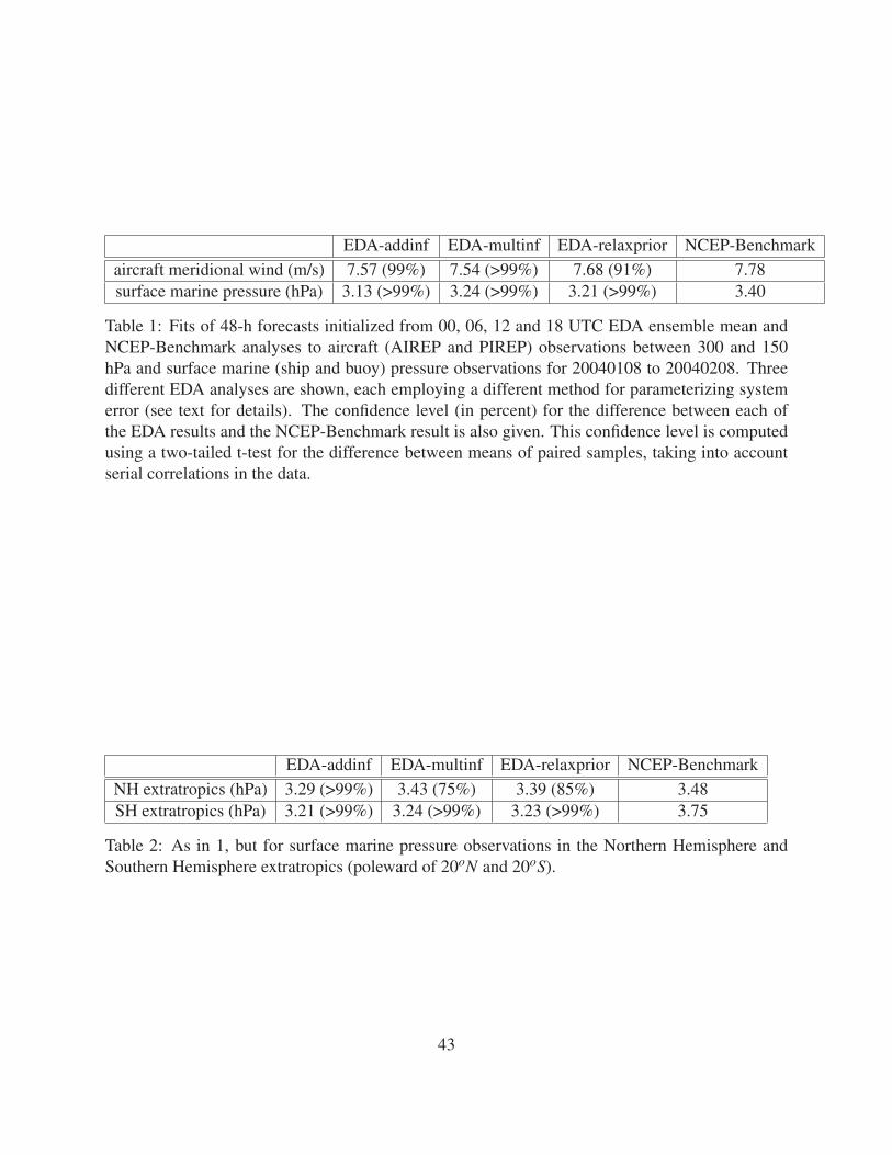
Table 1 shows the root-mean-square (RMS) fit of 48-h forecasts to marine surface pressure and

upper-tropospheric aircraft meridional wind observations. With the possible exception of the EDA-

relaxprior forecasts of meridional wind, the EDA-based forecasts fit the observations significantly

better than the NCEP-Benchmark forecasts. The significance level from a paired sample t-test

(Wilks 2006, p. 455) for the difference between the mean EDA forecast fits and the mean NCEP-

Benchmark forecast fits is also given in Table 1 for each of the EDA experiments. This significance

test takes into account serial correlations in the data by modeling the the sample differences as a

first-order autoregressive process. The significance level is then computed using an ’effective

sample size’ n′= n(1− r)/(1 + r) (Wilks 2006, p. 144), where n = 125 is the total sample size,

and r is the lag-1 autocorrelation of the forecast error differences. The EDA-addinf forecasts of

surface pressure appear to fit the observations better than the EDA-multinf and EDA-relaxprior

forecasts, although the differences between the EDA experiments are not significant at the 99%

confidence level.

Figure 2 shows the global RMS fit of 6 and 48-h forecasts to radiosonde profiles of meridional

wind and temperature for each of the experiments. With the exception of the EDA-relaxprior fore-

casts, the EDA-based forecasts fit the radiosonde observations at most levels better than the NCEP-

Benchmark forecasts. Aggregating all of the observations between σ = 0.9 and σ = 0.07, the dif-

20

ference between EDA-addinf and EDA-multinf and the NCEP-Benchmark forecasts is significant

at the 99% level. The EDA-relaxprior forecasts are not significantly closer to the radiosonde ob-

servations than the NCEP-Benchmark forecasts. The 48-h EDA-addinf forecasts generally have

the lowest error, although the differences between the EDA-addinf and EDA-multinf forecasts is

not statistically significant at the 99% level.

Table 2 shows the RMS fit of 48-h forecasts to marine surface pressure observations for the

Northern Hemisphere and the Southern Hemisphere separately. We have only stratified the results

by hemisphere for marine surface pressure because the other observation types are primarily con-

centrated in the Northern Hemisphere (Fig. 1). The difference between the fit of EDA forecasts

and NCEP-Benchmark forecasts to marine surface pressure observations is larger in the South-

ern Hemisphere extratropics than in the Northern Hemisphere extratropics (Table 2). This result

agrees with previous studies using EDA systems in a perfect-model context (Hamill and Snyder

2000) and using real observations characteristic of observing networks of the early 20th century

(Whitaker et al. 2004) which have shown that the flow-dependent background-error covariances

these systems provide have the largest impact when the observing network is sparse.

b. Verifications using analyses

When comparing forecasts and analyses from different centers, the standard practice in the

operational weather prediction community has been to verify each forecast against its own analysis,

that is, the analysis generated by the same center. The problem with this approach is that an analysis

can perform well in this metric if the assimilation completely ignores the observations. Here we

21

have the luxury of having an independent, higher quality analysis to verify against, the NCEP-

Operational analysis. Since this analysis was run at four times higher resolution and used a large

set of observations (including the satellite radiances), we expect it to be significantly better. We

have verified that this is indeed the case3, especially in the Southern Hemisphere where satellite

radiances have been found to have the largest impact on analysis quality (e.g. Derber and Wu 1998;

Simmons and Hollingsworth 2002).

Figure 3 shows vertical profiles of 48-hour geopotential height and meridional wind forecast

errors for both the Northern Hemisphere and Southern Hemisphere for forecasts initialized from

analyses produced by each of the EDA experiments and the NCEP-Benchmark experiment. Results

for zonal wind are very similar to meridional wind (not shown). For the most part, forecasts from

each of the EDA experiments track the NCEP-Operational analysis at 48 hours better than the

NCEP-Benchmark forecasts. The lone exception is the EDA-relaxprior forecasts of meridional

wind in the Northern Hemisphere. All the other EDA forecasts are more skillful than the NCEP-

Benchmark forecasts, and these differences are significant at the 99% level at 500 hPa, using the

paired-sample t-test for serially correlated data described previously. The EDA-addinf performs

better overall than the EDA-multinf and EDA-relaxprior experiments, although the differences are

only statistically significant at the 99% level in the Northern Hemisphere.

The improvement seen in the EDA experiments relative to the NCEP-Benchmark is especially

dramatic in the Southern Hemisphere, where Fig. 4 shows that it is equivalent to 24-hours of

lead time (in other words, 48-hour forecasts initialized from the EDA-addinf analyses are about

3by running forecasts run from the operational analysis with the same T62L28 version of the forecast model andcomparing those forecasts with radiosonde and marine surface pressure observations.

22

as accurate as 24-hour forecasts initialized from the NCEP-Benchmark 3D-Var analysis). In the

Northern Hemisphere, the advantage that the EDA-addinf based forecasts have over the NCEP-

Benchmark forecasts is closer to 6-h in lead time. This is further evidence that flow-dependent

covariances are most important in data sparse regions. This is illustrated for a specific case in Fig.

5, which shows the 500 hPa analyses produced by the NCEP-Benchmark, NCEP-Operational and

EDA-addinf analysis systems for 00 UTC February 3, 2004. The difference between the NCEP-

Benchmark and EDA-addinf analyses is especially large (greater than 100 m) in the trough off the

coast of Antarctica near 120oW , where the EDA-addinf is much closer to the NCEP-Operational

analysis. This region corresponds to the most data-sparse region of the Southern Hemisphere, as

can be seen from the distribution of marine surface pressure observations in Fig. 1. The EDA sys-

tem is clearly able to extract more information from the sparse Southern Hemisphere observational

network than the NCEP Benchmark system, and compares favorably with the higher-resolution

operational analysis which utilized more than an order of magnitude more observations in this

region (by assimilating satellite radiance measurements).

Since in-situ humidity measurements are quite sparse (in the NCEP GDAS system they are only

available from radiosondes), one might expect the ensemble-based data assimilation to show a clear

advantage over 3D-Var for the moisture field. Fig. 6 shows the RMS error of total precipitable wa-

ter forecasts for EDA-addinf and NCEP-Benchmark based forecasts. These forecasts are verified

against the higher-resolution NCEP operational analysis, which includes remotely sensed humidity

measurements. The EDA based forecasts have approximately 12-h advantage in lead time relative

to the 3D-Var based forecasts, in both the Northern and Southern Hemisphere extra-tropics. The

23

EDA systems can utilize non-moisture observations to make increments to the first-guess moisture

field through cross-covariances between the moisture field and the other state variables provided

by the ensemble. In the NCEP 3D-Var system, only observations of humidity can increment the

first-guess moisture field, since the static covariance model does not include cross-covariances be-

tween humidity and other state variables. Fig. 7 shows the increment of total precipitable water

implied by a single observation of surface pressure (show by the black dot) in the EDA-addinf

system for 00 UTC January 30, 2004. The EDA system is able to take into account the dynam-

ical relationship between the strength of the low center and the amplitude of the moisture plume

ahead of the cold front. An accurate, flow-dependent treatment of these dynamical relationships,

as represented by the cross-variable covariances in the ensemble, are particularly important in the

analysis of unobserved variables. Another example of this was given in the context of assimila-

tion of radar reflectivity into a cloud-resolving model by Snyder and Zhang (2003). In that study,

the cross-covariances between the predicted radar reflectivity and the other model state variables

(winds, temperature, moisture and condensate) provided by the ensemble were crucial in obtaining

an accurate analysis when only radar reflectivity was observed.

c. Ensemble Consistency

If the EDA system is performing optimally, the innovation covariances should satisfy

< (yo-Hxb)(yo-Hxb) >= HPbHT +R. (8)

24

(Houtekamer et al. 2005), where the angle brackets denote the expectation value. Here we com-

pare the diagonal elements of the matrices on the left and right hand sides of (8), computed for

radiosonde observations in the EDA experiments. If the magnitudes of those diagonal elements

are similar, the ensemble is said to be consistent, i.e., the innovation variances are consistent with

the background and observation error variances at the observation locations. This primarily re-

flects the degree to which parameterization of system error has been tuned, although with the small

number of parameters used here to represent system error it will be difficult if not impossible to

achieve a perfect match, unless the parameterization of system error itself is very accurate.

Figure 8 shows the square-root of the ensemble spread plus observation error variance (the

diagonal of the right-hand side of (8)) at radiosonde locations for the three EDA experiments.

This quantity can be regarded as the “predicted” innovation standard deviation, since if (8) is

satisfied, the two quantities will be the same. For the purposes of this discussion we will as-

sume that any disagreement between the left and right hand sides of (8) is due to deficiencies in

the background-error covariance, and not the observation-error covariance. The actual innova-

tion standard-deviation (or the root-mean-square fit) is shown in Fig. 8 only for the EDA-addinf

experiment, since the radiosonde fits for the other EDA experiments are quite similar. For both

temperature and meridional wind, the ensemble spread in the lower-troposphere is deficient for all

three EDA experiments. This means that all of the EDA systems are not making optimal use of the

radiosondes in the lower troposphere. In particular they are weighting the first guess too much.

Houtekamer et al. (2005) showed diagnostics similar to these for the MSC implementation of

the Ensemble Kalman Filter (their Fig. 5). The actual innovation standard deviations for their

25

implementation are quite similar to ours, but the predicted innovation standard deviations appear

to match the actual values more closely, particularly in the lower troposphere. In the MSC imple-

mentation, system error is additive and is derived from random samples drawn from a simplified

version of their operational background-error covariance model. The MSC operational covariance

itself has been tuned so that innovation statistics for the radiosonde network are consistent with

the observation and background error variance. Therefore, it is perhaps not surprising that the

vertical structure of the predicted innovation standard deviation more closely matches the actual

radiosonde innovations. In all three of our system error parameterizations, there is only one param-

eter that can be tuned (in the case of multiplicative inflation, this parameter can be tuned separately

in the Northern Hemisphere, Tropics and Southern Hemisphere). Therefore, the best that can be

done is to tune the parameterization so the global (or hemispheric) average predicted innovation

standard-deviation matches the actual. The fact that the vertical structure does not match means

that all of these system error parameterizations themselves are deficient, and do not correctly rep-

resent the vertical structure of the actual system error. In particular, the fact that the multiplicative

inflation system error parameterization cannot match the actual vertical structure of the innovation

variance suggests that the structure of the underlying system error covariance is quite different than

the background-error covariance represented by the dynamical ensemble, since the multiplicative

inflation parameterization can only represent the system error in the subspace of the existing en-

semble. One can either add more tunable parameters to the parameterizations to force the structures

to match, or try to develop new parameterizations that more accurately reflect the structure of the

underlying system error covariance.

26

Equation (8) is derived by assuming that the background forecast and observation errors are

uncorrelated, and the observations and background forecast are unbiased (i.e. the expected value

of the mean of the innovation yo-Hxb is zero). Figure 9 shows the innovation bias with respect

to radiosondes for the EDA-addinf and NCEP-Benchmark experiments (the other EDA experi-

ments (not shown) have similar innovation biases). There are significant temperature biases in

the lower troposphere, most likely due to systematic errors in the forecast model’s boundary-layer

parameterization. The temperature bias in the lower troposphere is a significant fraction of the

root-mean-square fit of the background forecast to the radiosonde observations (Fig. 2). Merid-

ional wind biases are also evident in the lower troposphere and near the tropopause, but are much

smaller relative to the root-mean-square fit. For the temperature field at least, the fact that the

ensemble spread appears deficient in the lower troposphere can be partially explained by the bias

component of the innovations, which is not accounted for in (8). However, the mismatch between

the predicted and actual meridional wind innovation standard deviation appears to primarily be a

result of deficiencies in the parameterization of the system error covariance.

d. Comparison with the LETKF

The Local Ensemble Transform Kalman Filter proposed by Hunt et al. (2006) is algorithmi-

cally very similar to the implementation used here, except that each state vector element is updated

using all the observations in the local region simultaneously using the Kalman Filter update equa-

tions expressed in the subspace of the ensemble. We have performed an experiment with LETKF

with observation error localization, using additive inflation as a parameterization of system er-

27

ror (LETKF-addinf). The parameter settings for the experiment are identical to those used in the

EDA-addinf experiment discussed previously. Figure 10 compares the 48-h geopotential height

and meridional wind forecast errors for forecasts initialized from the EDA-addinf, LETKF-addinf

and NCEP-Benchmark analyses. The skill of LETKF-addinf forecasts and EDA-addinf forecasts

are very similar. The small differences between the LETKF-addinf and EDA-addinf experiments

could be due to several factors. Firstly, the method used for localizing the impact of observations

is slightly different, the LETKF localizes the impact of observations by increasing the observa-

tion error with distance away from the analysis point, while our serial-processing implementation

localizes the background-error covariances directly. Further experimentation is needed to see if

these approaches are indeed equivalent in practice. Secondly, no adaptive observation thinning

was done in the LETKF experiment. The fact that the quality of the EDA-addinf and LETKF-

addinf forecasts are so similar in fact suggests that the adaptive observation thinning did not have

much of an impact, other than reducing the computational cost of the serial processing algorithm.

Regarding computational cost, we note that with the adaptive thinning algorithm, the cost of the

two algorithms are similar. If the adaptive thinning is turned off, the serial processing algorithm is

nearly an order of magnitude more expensive than the LETKF. Finally, we may not have tuned the

parameters to get the best performance from either the LETKF or the serial filter, and it is likely

that the optimal parameters are not the same. The differences between the the LETKF-addinf and

EDA-addinf experiments are so small that we believe differences in tuning, rather than fundamen-

tal differences in the algorithms, are more likely the primary factor.

28

4. Summary and Discussion

We have shown that ensemble data assimilation outperforms the NCEP operational 3D-Var

system, when satellite radiances are withheld and the forecast model is run at reduced resolution

(compared to NCEP operations). As expected from previous studies, the biggest improvement is

in data sparse regions. Since no satellite radiances were assimilated, the Southern Hemisphere is

indeed quite data sparse. The EDA analyses yielded a 24-hour improvement in geopotential height

forecast skill in the Southern Hemisphere extratropics relative to the NCEP 3D-Var system, so that

48-hour EDA-based forecasts are as accurate as 24-hour 3D-Var based forecasts. Improvements in

the data-rich Northern Hemisphere, while still statistically significant, were more modest (equiv-

alent to a 6-hour improvement in geopotential height forecast skill). For column integrated water

vapor, the EDA-based forecasts yielded at 12-h improvement in forecast skill in both the North-

ern and Southern Hemisphere extra-tropics. The fact that the improvement seen in the Northern

Hemisphere is larger for the moisture field than the temperature field is consistent with the fact that

in-situ measurements of humidity are sparse in both hemispheres. It remains to be seen whether

the magnitude of the improvements seen will be retained when satellite radiances are assimilated.

Three different parameterizations of system error (which is most likely dominated by model

error) were tested. All three performed similarly, but a parameterization based on additive inflation

using random samples of reanalysis 6-hour differences performed slightly better in our tests. All

the parameterizations tested failed to accurately predict the structure of the forecast innovation

variance, suggesting that further improvements in ensemble data assimilation may be achieved

when methods for better accounting for the covariance structure of system error are developed.

29

Significant innovation biases were found, primarily for lower tropospheric temperature, suggesting

that bias removal algorithms for EDA (such as those proposed by Baek et al. (2006) and Keppenne

et al. (2005)) could also significantly improve the performance of EDA systems.

We believe that these results warrant accelerated development of ensemble data assimilation

systems for operational weather prediction. The limiting factor in the performance of these systems

is almost certainly the parameterization of system error. Even without further improvements in

the parameterization of model error, ensemble data assimilation systems should become more

and more accurate relative to 3D-Var systems as forecast models improve and the amplitude of

the model-error part of the background-error covariance decreases. Current generation ensemble

data assimilation systems are computationally competitive with their primary alternative, 4D-Var.

However, they are considerably simpler to code and maintain, since an adjoint of the forecast

model is not needed.

Acknowledgments

Fruitful discussions with C. Bishop, E. Kalnay, J. Anderson, I. Szyunogh, P. Houtekamer, F.

Zhang, G. Compo, H. Mitchell and B. Hunt are gratefully acknowledged, as are the comments of

three anonymous reviewers. This project would not have been possible without the support of the

NOAA THORPEX program, which partially funded this research through a grant, and NOAA’s

Forecast Systems Laboratory, which provided access to their High Performance Computing Sys-

tem. One of us (Hamill) was partially supported through the National Science Foundation grants

ATM-0130154 and ATM-020561.

30

Appendix: Re-tuning the NCEP GDAS background error.

The background error covariances in the NCEP GDAS were originally obtained using the so-

called ’NMC method’ (Parrish and Derber 1992). This method assumes the statistics of back-

ground error can be estimated from the covariances of differences between 48 and 24 hour fore-

casts verifying at the same time. The background-error covariances used in the operational GDAS

were obtained using T254L64 forecasts, initialized from an analysis that included satellite radi-

ances. In order to retune the system for T62L28 resolution, we re-ran the ’NMC method’ using

the difference between 48- and 24-hour T62L28 forecasts, initialized from the operational anal-

yses for January and February 2004. Figure 11 shows the 48-hour forecast skill (relative to the

operational analysis) for forecasts initialized from a NCEP GDAS T62L28 assimilation without

satellite radiances. The solid curve denotes the skill of forecasts initialized from analyses gener-

ated with the operational background-error statistics, while the dashed curve denotes the skill of

forecasts initialized from analyses generated with the new background-error statistics. Re-tuning

the background-error statistics improves the forecasts in the Southern Hemisphere, but degrades

the forecasts in the Northern Hemisphere. Further iterations of the NMC method (using 48- minus

24-h forecasts initialized from analyses produced by the previous iteration) do not improve the

forecast skill.

Since our attempt to retune the background-error statistics using the ’NMC method’ did not

uniformly improve the analyses, we tried an alternative approach. In the Spectral Statistical Inter-

polation (SSI) system used in the NCEP GDAS, the structure of the background-error covariances

are the same everywhere over the globe. However, the amplitude of the background-error vari-

31

ances may vary with latitude. If we assume that the dominant effect of removing the satellite

radiances and reducing the resolution of the forecast model is to modify the amplitude of the back-

ground error in the Southern Hemisphere, without changing the structure of the background-error

covariance, then modifying the latitudinally varying background-error variances in the Southern

Hemisphere should improve the quality of the analyses there, without degrading the analyses in

the Northern Hemisphere. Following this logic, we multiply the operational background error

variances by the function

1 φ≥ 0

1+bsin2φ φ < 0(9)

where φ is latitude and b is an arbitrary constant factor that controls the amplitude in the Southern

Hemisphere extra-tropics. By numerical experimentation (running the assimilation for one month,

and examining the skill of 48-hour forecasts relative to the operational analysis) we have found

that b = −0.75 produces the best results4. Figure 12 shows the skill of 48-hour geopotential

height forecasts for the T62L28 ’no-sat’ experiments, using the operational (solid line) and retuned

(dashed line) background error variances. The ’no-sat’ forecast error is reduced by 13% at 500 hPa

in the Southern Hemisphere, and the forecast skill in Northern Hemisphere is changed little. We

have used these analyses, which we refer to as the ’NCEP-Benchmark’ analyses, throughout this

study as a yardstick to measure EDA performance.

4A negative value of the b parameter implies that the background error variance is reduced in the Southern Hemi-sphere relative to the operational value. This is a somewhat surprising result, since we expected the background errorvariance would need to be increased for the ’no-sat’ observation network. Independent calculations performed atNCEP by one of the coauthors (Y. Song) have confirmed that that analyses excluding satellite radiances are degradedwhen b > 0.

32

References

Anderson, J. L., 2001: An ensemble adjustment Kalman filter for data assimilation. Mon. Wea.

Rev., 129, 2884–2903.

Anderson, J. L. and S. L. Anderson, 1999: A Monte Carlo implementation of the nonlinear filtering

problem to produce ensemble assimilations and forecasts. Mon. Wea. Rev., 127, 2741–2758.

Baek, S.-J., B. R. Hunt, E. Kalnay, E. Ott, and I. Szunyogh, 2006: Local ensemble Kalman filtering

in the presence of model bias. Tellus A, 58, 293–306.

Bishop, C. H., B. Etherton, and S. J. Majumdar, 2001: Adaptive sampling with the ensemble

transform Kalman filter. Part I: Theoretical Aspects. Mon. Wea. Rev., 129, 420–436.

Bouttier, F., 1994: A dynamical estimation of forecast error covariances in an assimilation system.

Mon. Wea. Rev., 122, 2376–2390.

Burgers, G., P. J. van Leeuwen, and G. Evensen, 1998: Analysis scheme in the ensemble Kalman

filter. Mon. Wea. Rev., 126, 1719–1724.

Compo, G. P., J. S. Whitaker, and P. D. Sardeshmukh, 2006: Feasibility of a 100 year reanalysis

using only surface pressure data. Bull. Amer. Meteor. Soc., 87, 175–190.

Courtier, P., J.-N. Thépaut, and A. Hollingsworth, 1994: A strategy for operational implementation

of 4D-Var, using an incremental approach. Quart. J. Roy. Meteor. Soc., 120, 1367–1387.

Daley, R., 1991: Atmospheric Data Analysis. Cambridge University Press, 457 pp.

33

Derber, J. and W.-S. Wu, 1998: The use of TOVS cloud-cleared radiances in the NCEP SSI analysis

system. Mon. Wea. Rev., 2287–2299.

Evensen, G., 2003: The Ensemble Kalman Filter: Theoretical formulation and practical imple-

mentation. Ocean Dynamics, 53, 343–367.

Gaspari, G. and S. E. Cohn, 1999: Construction of correlation functions in two and three dimensio

ns. Quart. J. Roy. Meteor. Soc., 125, 723–757.

Gelb, A., J. F. Kasper, R. A. Nash, C. F. Price, and A. A. Sutherland, 1974: Applied Optimal

Estimation. M. I. T. Press, 374 pp.

Global Climate and Weather Modeling Branch, Environmental Modeling Center, 2003: The GFS

Atmospheric Model. Office Note 442, NCEP, NOAA/National Weather Service National Cen-

ters for Environmental Prediction, Environmental Modelling Center, 5200 Auth Road, Camp

Springs, MD 20746.

URL http://www.emc.ncep.noaa.gov/officenotes/FullTOC.html

Hamill, T. M., 2006: Ensemble-based data assimilation. Predicability of Weather and Climate,

Cambridge Press, chapter 6, 124–156.

Hamill, T. M. and C. Snyder, 2000: A hybrid ensemble Kalman filter-3d variational analysis

scheme. Mon. Wea. Rev., 128, 2905–2919.

Hamill, T. M. and J. S. Whitaker, 2005: Accounting for the error due to unresolved scales in

ensemble data assimilation: A comparison of different approaches. Mon. Wea. Rev., 133, 3132–

3147.

34

Hamill, T. M., J. S. Whitaker, and C. Snyder, 2001: Distance-dependent filtering of background

error covariance estimates in an ensemble Kalman filter. Mon. Wea. Rev., 129, 2776–2790.

Houtekamer, P., L. Lefaivre, J. Derome, H. Ritchie, and H. L. Mitchell, 1996: A system simulation

approach to ensemble prediction. Mon. Wea. Rev., 124, 1225–1242.

Houtekamer, P. L. and H. L. Mitchell, 1998: Data assimilation using an ensemble Kalman filter

technique. Mon. Wea. Rev., 126, 796–811.

— 2001: A sequential ensemble Kalman filter for atmospheric data assimilation. Mon. Wea. Rev.,

129, 123–137.

— 2005: Ensemble Kalman Filtering. Quart. J. Roy. Meteor. Soc., 131, 3269–3289.

Houtekamer, P. L., H. L. Mitchell, G. Pellerin, M. Buehner, M. Charron, L. Spacek, and B. Hansen,

2005: Atmospheric data assimilation with an Ensemble Kalman Filter: Results with real obser-

vations. Mon. Wea. Rev., 133, 604–620.

Hunt, B., E. Kostelich, and I. Syzunogh, 2006: Efficient data assimilation for spatio-temporal

chaos: A local ensemble transform Kalman filter. Physica D, submitted.

URL http://arxiv.org/abs/physics/0511236

Ide, K., P. Courtier, M. Ghil, and A. C. Lorenc, 1997: Unified notation for data assimilation:

operational, sequential, and variational. J. Met. Soc. Japan, 75 (1B), 181–189.

Kalnay, E., L. Hong, T. Miyoshi, S.-C. Yang, and J. Ballabrera, 2007: 4d-Var or Ensemble Kalman

Filter? Tellus, submitted.

35

Kaminski, P. G., J. A. E. Bryson, and S. F. Schmidt, 1971: Discrete square-root filtering: a survey

of current techniques. IEEE T. Automat. Control, AC-16, 727–736.

Keppenne, C. L., M. M. Rienecker, N. P. Kurkowski, and D. A. Adamec, 2005: Ensemble Kalman

filter assimilation of temperature and altimeter data with bias correction and application to sea-

sonal prediction. Nonlinear Processes in Geophysics, 12, 491–503.

Kistler, R., E. Kalnay, W. Collins, S. Saha, G. White, J. Woollen, M. Chelliah, W. Ebisuzaki,

M. Kanamitsu, V. Kousky, H. van den Dool, R. Jenne, and M. Fiorino, 2001: The NCEP-NCAR

50-Year Reanalysis: Monthly Means CD-ROM and Documentation. Bull. Amer. Meteor. Soc.,

82, 247–268.

Liu, Z.-Q. and F. Rabier, 2002: The interaction between model resolution, observation resolution

and observation density in data assimilation: A one-dimensional study. Quart. J. Roy. Meteor.

Soc., 128, 1367–1386.

Lorenc, A. C., 1986: Analysis methods for numerical weather prediction. Quart. J. Roy. Meteor.

Soc., 112, 1177–1194.

Lynch, P. and X.-Y. Huang, 1992: Initialization of the HIRLAM model using a digital filter. Mon.

Wea. Rev., 120, 1019–1034.

Meng, Z. and F. Zhang, 2007: Tests of an ensemble Kalman filter for mesoscale and regional-scale

data assimilation. Part II: Imperfect model experiments. Mon. Wea. Rev., in press.

Miyoshi, T. and S. Yamane, 2006: Local ensemble transform Kalman filtering with an AGCM at

T159/L60 resolution. Mon. Wea. Rev., submitted.

36

NCEP Environmental Modeling Center, 2004: SSI Analysis System 2004. Office Note 443, NCEP,

NOAA/National Weather Service National Centers for Environmental Prediction, Environmen-

tal Modelling Center, 5200 Auth Road, Camp Springs, MD 20746.

URL http://www.emc.ncep.noaa.gov/officenotes/FullTOC.html

Ochotta, T., C. Gebhardt, D. Saupe, and W. Wergen, 2005: Adaptive thinning of atmospheric

observations in data assimilation with vector quantization and filtering methods. Quart. J. Roy.

Meteor. Soc., 131, 3427–3437.

Oppenheim, A. and R. W. Schafer, 1989: Discrete-Time Signal Processing. Prentice-Hall, 879 pp.

Ott, E., B. R. Hunt, I. Szunyogh, A. Zimin, E. Kostelich, M. Corazza, E. Kalnay, D. Patil, and J. A.

Yorke, 2004: A local Ensemble Kalman Filter for atmospheric data assimilation. Tellus, 56A,

415–428.

Parrish, D. and J. Derber, 1992: The National Meteorological Center’s spectral statistical interpo-

lation analysis system. Mon. Wea. Rev., 120, 1747–1763.

Pires, C., R. Vautard, and O. Talagrand, 1996: On extending the limits of variational assimilation

in nonlinear chaotic systems. Tellus, 48A, 96–121.

Rabier, F., H. Järvinen, E. Klinker, J.-F. Mafouf, and A. Simmons, 2000: The ECMWF operational

implementation of four-dimensional variational assimilation. Quart. J. Roy. Meteor. Soc., 126,

1143–1170.

Simmons, A. J. and A. Hollingsworth, 2002: Some aspects of the improvement in skill of numeri-

cal weather prediction. Quart. J. Roy. Meteor. Soc., 128, 647–677.

37

Snyder, C. and F. Zhang, 2003: Assimilation of simulated doppler radar observations with an

ensemble Kalman filter. Mon. Wea. Rev., 131, 1663–1677.

Thépaut, J.-N. and . P. Courtier, 1991: Four-dimensional data assimilation using the adjoint of a

multilevel primitive equation model. Quart. J. Roy. Meteor. Soc., 117, 1225–1254.

Tippett, M. K., J. L. Anderson, C. H. Bishop, T. M. Hamill, and J. S. Whitaker, 2003: Ensemble

Square Root Filters. Mon. Wea. Rev., 131, 1485–1490.

Whitaker, J. S., G. P. Compo, and T. M. Hamill, 2004: Reanalysis without radiosondes using

ensemble data assimilation. Mon. Wea. Rev., 132, 1190–1200.

Whitaker, J. S. and T. M. Hamill, 2002: Ensemble data assimilation without perturbed observa-

tions. Mon. Wea. Rev., 130, 1913–1924.

Wilks, D. S., 2006: Statistical Methods in the Atmospheric Sciences. Academic Press, 467 pp.,

second edition.

Zhang, F., C. Snyder, and J. Sun, 2004: Impacts of initial estimate and observation availability

on convective-scale data assimilation with an Ensemble Kalman Filter. Mon. Wea. Rev., 132,

1238–1253.

38

Figure Captions

Figure 1: Locations of (A) radiosonde observations, (B) aircraft observations (AIREP

and PIREP observations between 300 and 150 hPa), and (C) surface marine (ship

and buoy) pressure observations for 00 UTC and 12 UTC January 10, 2004. 44

Figure 2: Root-mean-square fits of 6 and 48-h forecasts initialized from 00, 06, 12

and 18 UTC EDA ensemble mean and NCEP-Benchmark analyses to radiosonde

observations for 20040108 to 20040208. Three different EDA analyses are shown,

each employing a different method for parameterizing system error (see text for

details). Note that the ordinate is sigma layer, not pressure level, since the calcula-

tions were done in sigma coordinates. There is one data point for each interval of

width ∆σ = 0.1, beginning at σ = 0.9, representing all of the observations in each

layer. 45

Figure 3: Vertical profiles of 48-hour forecast error (measured relative to the NCEP-

Operational analysis). Values for the Northern Hemisphere (poleward of 20oN)

and the Southern Hemisphere (poleward of 20oS) are shown for geopotential height

and meridional wind, for each of the EDA experiments and the NCEP-Benchmark

experiment. 46

39

Figure 4: 500 hPa geopotential height forecast error (measured relative to the NCEP-

Operational analysis) as a function of forecast lead time, for the Northern and

Southern Hemisphere extra-tropics (the region poleward of 20o). The thinner curve

is for forecast initialized from the ensemble mean EDA-addinf analysis, and the

thicker curve is for forecasts initialized from the NCEP-Benchmark analysis. 47

Figure 5: February 3, 2004 00 UTC Southern Hemisphere 500 hPa geopotential height

analyses for the EDA-addinf (A), the NCEP-Benchmark (B), and the NCEP-Operational

(C) analysis systems. The difference between the EDA-addinf and NCEP-Benchmark

analyses is shown in (D). The contour interval is 75 m in (A)-(C) and 40 m in (D).

The 5125 and 5425 meter contours are emphasized in (A)-(C). All contours in (D)

are negative. 48

Figure 6: As in Figure 4, but for total precipitable water (in mm). 49

Figure 7: Precipitable water analysis increment (thick black contour lines, contour

interval 0.5 mm, dashed lines negative, zero contour suppressed) from the EDA-

addinf system at 00 UTC January 30, 2004 associated with a surface pressure

observation located at the black dot at the center of the map. The surface pressure

observation is 1 hPa lower than the ensemble mean first-guess forecast (thin black

contours, interval 5 hPa). The gray-shaded field is the ensemble mean first-guess

precipitable water (scale on right denotes contour levels). 50

40

Figure 8: Square-root of ensemble spread plus observation error variance at radiosonde

locations for 6-h forecasts initialized from 06 UTC and 18 UTC EDA for 20040108

to 20040208. Three different EDA ensembles are shown, each employing a dif-

ferent method for parameterizing system error (see text for details). The root-

mean-square fit of the 6-h EDA-addinf ensemble mean forecast to the radiosonde

observations is also shown (heavy solid curve). 51

Figure 9: Mean difference between 6-h forecast and radiosonde observations (bias)

for forecasts initialized from 06 UTC and 18 UTC EDA for 20040108 to 20040208.

Three different EDA ensembles are shown, each employing a different method for

parameterizing system error (see text for details). 52

Figure 10: Vertical profiles of 48-hour geopotential height and meridional wind fore-

cast error (measured relative to the NCEP-Operational analysis). Values for the

Northern Hemisphere (poleward of 20oN) and the Southern Hemisphere (poleward

of 20oS) are shown for the EDA-addinf, LETKF-addinf and the NCEP-Benchmark

experiments. 53

41

Figure 11: Vertical profiles of 48-hour forecast error, measured relative to the NCEP-

Operational analysis, in the Northern and Southern Hemisphere extratropics (pole-

ward of 20oS). Forecasts were initialized four times daily between 2004010800

and 2004020800 from analyses that did not include satellite radiances. The solid

line is for T62L28 forecasts initialized from a T62L28 run of the NCEP GDAS

system, but using the operational background-error covariances (which were tuned

for a T256L64 forecast model and an observing network that includes satellite radi-

ances). The dashed line is for T62L28 forecasts initialized from a run of the NCEP

GDAS at T62L28 resolution, using background-error covariances determined from

the difference between 48- and 24-hour T62L28 forecasts via the ’NMC method’. 54

Figure 12: As in Figure 11, except that the thick dashed line represents T62L28 fore-

casts initialized from a T26L28 run of the NCEP GDAS system with the background-

error variances modified only in the Southern Hemisphere, as described in the Ap-

pendix. 55

42

EDA-addinf EDA-multinf EDA-relaxprior NCEP-Benchmarkaircraft meridional wind (m/s) 7.57 (99%) 7.54 (>99%) 7.68 (91%) 7.78surface marine pressure (hPa) 3.13 (>99%) 3.24 (>99%) 3.21 (>99%) 3.40

Table 1: Fits of 48-h forecasts initialized from 00, 06, 12 and 18 UTC EDA ensemble mean andNCEP-Benchmark analyses to aircraft (AIREP and PIREP) observations between 300 and 150hPa and surface marine (ship and buoy) pressure observations for 20040108 to 20040208. Threedifferent EDA analyses are shown, each employing a different method for parameterizing systemerror (see text for details). The confidence level (in percent) for the difference between each ofthe EDA results and the NCEP-Benchmark result is also given. This confidence level is computedusing a two-tailed t-test for the difference between means of paired samples, taking into accountserial correlations in the data.

EDA-addinf EDA-multinf EDA-relaxprior NCEP-BenchmarkNH extratropics (hPa) 3.29 (>99%) 3.43 (75%) 3.39 (85%) 3.48SH extratropics (hPa) 3.21 (>99%) 3.24 (>99%) 3.23 (>99%) 3.75

Table 2: As in 1, but for surface marine pressure observations in the Northern Hemisphere andSouthern Hemisphere extratropics (poleward of 20oN and 20oS).

43

��������������������� �� � ��� � �� � ��

��������������������� ���� ��� � �� � ��

�������������������� ���� ����� ���� ����� ������� ����� ������ ������� � �� � ��

Figure 1: Locations of (A) radiosonde observations, (B) aircraft observations (AIREP and PIREPobservations between 300 and 150 hPa), and (C) surface marine (ship and buoy) pressure observa-tions for 00 UTC and 12 UTC January 10, 2004.

44

��� ��� ��� ��� ��� ��� ��������������������������������� ���� ����

���������� ����� �!" � #$%&��� �� �� � ��� �� �� �'()(*+ ,(* +(-./0

����������������������������� ���� �������������� 1� ������2 3��� #$%&

45678009/:4567';<)9/:4567*(<8=,*9.*>?4@7A(/-B'8*C��� ��� ��� ��� ��� ��� ��� ��� ����

����������������������������� ���� �������������� ����� �!" � D%&

��� �� ��� ��'()(*+ ,(* +(-./0����������������������������� ���� ����

���������� 1� ������2 3��� D%&

Figure 2: Root-mean-square fits of 6 and 48-h forecasts initialized from 00, 06, 12 and 18 UTCEDA ensemble mean and NCEP-Benchmark analyses to radiosonde observations for 20040108to 20040208. Three different EDA analyses are shown, each employing a different method forparameterizing system error (see text for details). Note that the ordinate is sigma layer, not pressurelevel, since the calculations were done in sigma coordinates. There is one data point for eachinterval of width ∆σ = 0.1, beginning at σ = 0.9, representing all of the observations in each layer.

45

�� �� �� �� ���

����������������������������� ���� � ���� � ���� ����������� ���!"�

#$%&'()*+,-./0%12'.334*5%12'-6784*5%12'/)7.9:/4;/ �� �� �� �� �� ���

����������������������������� ���� � ���<� ���� ����������� ���!"�

�=� �=� �=� �=� �=� �=� �=� �=� �=��>?>@A B>@ A>CDEF

����������������������������� ���� � ���� � ���� G�H�I���� J��I

� � � � � �>?>@A B>@ A>CDEF

����������������������������� ���� � ���<� ���� G�H�I���� J��I

Figure 3: Vertical profiles of 48-hour forecast error (measured relative to the NCEP-Operationalanalysis). Values for the Northern Hemisphere (poleward of 20oN) and the Southern Hemisphere(poleward of 20oS) are shown for geopotential height and meridional wind, for each of the EDAexperiments and the NCEP-Benchmark experiment.

46

�� �� �� �� �� ����� �� ���������������������� ����� ���� ���

� !"#$%#$&'()*�� �� �� �� �� ����� �� ������������

�������������� ����� ���� ���+ !"#$%#$&'()*

,-./01123456,7 893:;<0=>Figure 4: 500 hPa geopotential height forecast error (measured relative to the NCEP-Operationalanalysis) as a function of forecast lead time, for the Northern and Southern Hemisphere extra-tropics (the region poleward of 20o). The thinner curve is for forecast initialized from the ensem-ble mean EDA-addinf analysis, and the thicker curve is for forecasts initialized from the NCEP-Benchmark analysis.

47

�����������

��� ��� ��� ����������

������������������������� ��������

�����������

������������ �!��� ����������

���������"#$% &'()

�� ��� ��� ���*��������������

+,,-,+,.,,

Figure 5: February 3, 2004 00 UTC Southern Hemisphere 500 hPa geopotential height analyses forthe EDA-addinf (A), the NCEP-Benchmark (B), and the NCEP-Operational (C) analysis systems.The difference between the EDA-addinf and NCEP-Benchmark analyses is shown in (D). Thecontour interval is 75 m in (A)-(C) and 40 m in (D). The 5125 and 5425 meter contours areemphasized in (A)-(C). All contours in (D) are negative.

48

�� �� �� �� �� ����� �� ������������������������������ ����� ���

�� �� !" !#$%&'�� �� �� �� �� ����� �� �������(�����((��(�(���

���� ����� ���)� �� !" !#$%&'*+,-.//01234*5 67189:.;<

Figure 6: As in Figure 4, but for total precipitable water (in mm).

49

���� ������������� ���� ���

���������������� ����� ���� !�! "����#��� $%%&%'(%%%

)*)+),)-).)

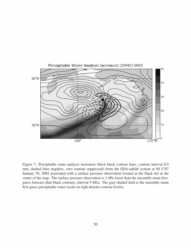
Figure 7: Precipitable water analysis increment (thick black contour lines, contour interval 0.5mm, dashed lines negative, zero contour suppressed) from the EDA-addinf system at 00 UTCJanuary 30, 2004 associated with a surface pressure observation located at the black dot at thecenter of the map. The surface pressure observation is 1 hPa lower than the ensemble mean first-guess forecast (thin black contours, interval 5 hPa). The gray-shaded field is the ensemble meanfirst-guess precipitable water (scale on right denotes contour levels).

50

��� ��� ��� ��� ��� ��� ��� ��� ��������������������������������� ���� �� ���

��� ���������� �!"�#�$%#�&'()*++,-.&'()/012,-.&'()341*563,738,2 9&'()*++,-.:

��� �� ��� �� ��� �� ��/4243; 643 ;4<7-+����������������������������� ���� �� ����=� ���������� >�#������?@���

Figure 8: Square-root of ensemble spread plus observation error variance at radiosonde locationsfor 6-h forecasts initialized from 06 UTC and 18 UTC EDA for 20040108 to 20040208. Threedifferent EDA ensembles are shown, each employing a different method for parameterizing systemerror (see text for details). The root-mean-square fit of the 6-h EDA-addinf ensemble mean forecastto the radiosonde observations is also shown (heavy solid curve).

51

���� ���� ��� ��� ������������������������� ��� ������� ���������� �� !�"�#$"�

%&'()**+,-%&'(./01+,-%&'(230)452+6278%9(:3,;<.)2=

���� ���� ��� ��� ���.3132> 532 >3;6,*��������������������� ��� ������� ���������� ?�"������@A���

Figure 9: Mean difference between 6-h forecast and radiosonde observations (bias) for forecastsinitialized from 06 UTC and 18 UTC EDA for 20040108 to 20040208. Three different EDAensembles are shown, each employing a different method for parameterizing system error (see textfor details).

52

�� �� �� �� ���

����������������������������� ���� � ���� � ���� ����������� ���!"�

�#$% &��'"��()$*+,�--��./$012,�--��. �� �� �� �� �� ���

����������������������������� ���� � ���3� ���� ����������� ���!"�

�4� �4� �4� �4� �4� �4� �4� �4� �4��56578 957 85:;<=

����������������������������� ���� � ���� � ���� >�(�-���� ?��-

� � � � � �56578 957 85:;<=

����������������������������� ���� � ���3� ���� >�(�-���� ?��-

Figure 10: Vertical profiles of 48-hour geopotential height and meridional wind forecast error(measured relative to the NCEP-Operational analysis). Values for the Northern Hemisphere (pole-ward of 20oN) and the Southern Hemisphere (poleward of 20oS) are shown for the EDA-addinf,LETKF-addinf and the NCEP-Benchmark experiments.

53

�� �� �� �� �� �� ���

����������������������������� ���� � ���� � ���� ����������� ���!"�

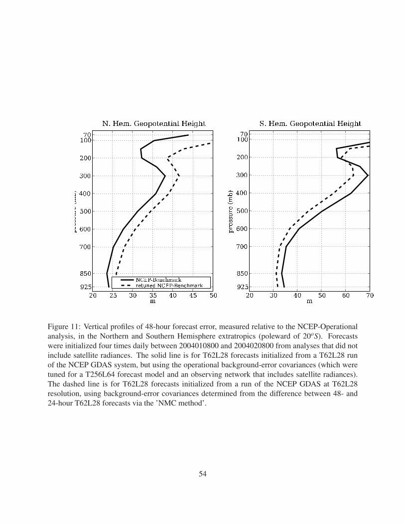
#$%&'()*+,-./0/)12*)3 #$%&'()*+,-./0 �� �� �� �� �� ���

����������������������������� ���� � ���4� ���� ����������� ���!"�

Figure 11: Vertical profiles of 48-hour forecast error, measured relative to the NCEP-Operationalanalysis, in the Northern and Southern Hemisphere extratropics (poleward of 20oS). Forecastswere initialized four times daily between 2004010800 and 2004020800 from analyses that did notinclude satellite radiances. The solid line is for T62L28 forecasts initialized from a T62L28 runof the NCEP GDAS system, but using the operational background-error covariances (which weretuned for a T256L64 forecast model and an observing network that includes satellite radiances).The dashed line is for T62L28 forecasts initialized from a run of the NCEP GDAS at T62L28resolution, using background-error covariances determined from the difference between 48- and24-hour T62L28 forecasts via the ’NMC method’.

54

�� �� �� �� �� �� ���

����������������������������� ���� � ���� � ���� ����������� ���!"�

#$%&'()*+,-./0/)12*)3 #$%&'()*+,-./0 �� �� �� �� �� ���

����������������������������� ���� � ���4� ���� ����������� ���!"�

Figure 12: As in Figure 11, except that the thick dashed line represents T62L28 forecasts initializedfrom a T26L28 run of the NCEP GDAS system with the background-error variances modified onlyin the Southern Hemisphere, as described in the Appendix.

55