Dense Structure From A Dense Optical FlowSequence

Yalin Xiong Steven A. Shafer

CMU-RI-TR-95-10

The Robotics InstituteCarnegie Mellon University

Pittsburgh, Pennsylvania 15213

April, 1995

c 1995 Carnegie Mellon University

Contents

1 Introduction 1

2 System Overview 2

2.1 Coordinates and Motion : : : : : : : : : : : : : : : : : : : : : : : : : 22.2 Block Diagram of the System : : : : : : : : : : : : : : : : : : : : : : 3

3 EKF-based Uncertainty Update 3

3.1 Decomposition of Independent and Correlated Uncertainty : : : : : : 63.2 Weighted Principal Component Analysis : : : : : : : : : : : : : : : : 8

4 Initial Motion Estimation 12

4.1 Dynamic Motion Parameterization : : : : : : : : : : : : : : : : : : : 12

5 Interpolation and Forward Transformation 13

6 Implementation Issues and Experiments 16

6.1 Implementation Issues : : : : : : : : : : : : : : : : : : : : : : : : : : 166.2 Experiments : : : : : : : : : : : : : : : : : : : : : : : : : : : : : : : : 17

6.2.1 Ambiguities : : : : : : : : : : : : : : : : : : : : : : : : : : : : 176.2.2 Experiments on Real Sequences : : : : : : : : : : : : : : : : : 23

7 Summary 29

A Sherman-Morrison-Woodbury Inversion 30

B Eigen Analysis of Symmetric Outer Products 31

I

List of Figures

1 The Camera Coordinate : : : : : : : : : : : : : : : : : : : : : : : : : 22 Block Diagram of The System : : : : : : : : : : : : : : : : : : : : : : 43 An Image Sequence of A Toy House : : : : : : : : : : : : : : : : : : : 104 Six Non-Weighted Principal Components : : : : : : : : : : : : : : : : 115 Six Weighted Principal Components : : : : : : : : : : : : : : : : : : : 116 Vector Field as Correlated Uncertainty : : : : : : : : : : : : : : : : : 147 One Frame in A Strawhat Sequence : : : : : : : : : : : : : : : : : : : 198 Three Eigenimages For the Strawhat Sequence : : : : : : : : : : : : : 199 Evolutions of Strawhat Uncertainties : : : : : : : : : : : : : : : : : : 2010 A Road Sequence : : : : : : : : : : : : : : : : : : : : : : : : : : : : : 2111 The First Three Eigenimages of the Road Sequence : : : : : : : : : : 2112 Evolutions of Road Uncertainties : : : : : : : : : : : : : : : : : : : : 2213 The Straw Hat Sequence : : : : : : : : : : : : : : : : : : : : : : : : : 2414 The Chair Sequence : : : : : : : : : : : : : : : : : : : : : : : : : : : : 2515 The Cube Sequence : : : : : : : : : : : : : : : : : : : : : : : : : : : : 2616 The Basket Sequence : : : : : : : : : : : : : : : : : : : : : : : : : : : 2717 The Sphere and Dog Sequence : : : : : : : : : : : : : : : : : : : : : : 28

II

Abstract

This paper presents a structure-from-motion system which delivers dense structureinformation from a sequence of dense optical ows. Most traditional feature-basedapproaches cannot be extended to compute dense structure due to impractical com-putational complexity. We demonstrate that by decomposing uncertainty informationinto independent and correlated parts we can decrease these complexities from O(N2)to O(N), where N is the number of pixels in the images. We also show that this densestructure-from-motion system requires only local optical ows, i.e. image matchingsbetween two adjacent frames, instead of the tracking of features over a long sequenceof frames.

III

1 Introduction

Structure from motion has been one of the most active areas in computer visionduring the past decade. The idea is to recover structure or shape information froma sequence of images taken under unknown relative motions between the camera andthe scene. Most approaches proposed in the literature can be classi�ed according towhether they are based upon features or optical ows.

Feature-based methods compute the relative structure information among featuresby analyzing their 2D motion in images. Examples of such systems are reported byTsai & Huang [19], Tomasi & Kanade [18], Broida et al [5] and Azarbayejani &Pentland [3] . Because the whole analysis is limited to features which usually numbernot more than hundreds, the results from those systems yield very sparse shapeinformation. While stripping a full-resolution image to a handful of features maygreatly simplify the algorithm and the computation, most of information containedin the image is lost. In many applications such as model acquisition, inspection andnavigation, dense structural information is more desirable.

Traditional ow-based methods, such as reported by Bruss & Horn [6], Weng et al[20], Heeger & Jepson [11], Adiv [1], have concentrated on either solving the problemof recovering motion and structure from a single optical ow �eld or using very lowresolution optical ows. As far as we know, little has been done to achieve a densestructure-from-motion system except Heel's work in [13]. Unfortunately, as pointedout in [18] that whether the proposed iterative algorithm in [18] converges is still anopen question. Overall, the di�culties of such a system arise from two main factors:

� Computation. While a feature-based method can easily a�ord an O(N2) orO(N 3) algorithm, whereN is the number of features, a ow-based method cannoteven a�ord an O(N2) algorithm, where N is the number of pixels.

� Accumulation. While a feature-based method can accumulate structural infor-mation for features because they are tracked across many frames, optical owsusually cannot be used to track pixels because their measurements are uncertain.In other words, while a feature-based approach quantify the image informationas either totally unreliable or very reliable, a ow-based approach has to usea spectrum of reliability. Therefore, it is impossible to accumulate structuralinformation by tracking all pixels across many frames in a ow-based method.

This paper shows our attempt at overcoming these di�culties. We demonstrate asystem which incrementally accumulates dense structural information from a sequenceof optical ows. The system has the following features:

� The system is based on EKF (extended Kalman �ltering) as proposed in [5]. Wewill show in our experiment that the nonlinearity problem is actually not veryserious even when the initial data are very crude.

� The formulation of the structure from motion uses separate independent andcorrelated structure uncertainty estimations. By employing the separation and

1

x

y

z

Image Plane O

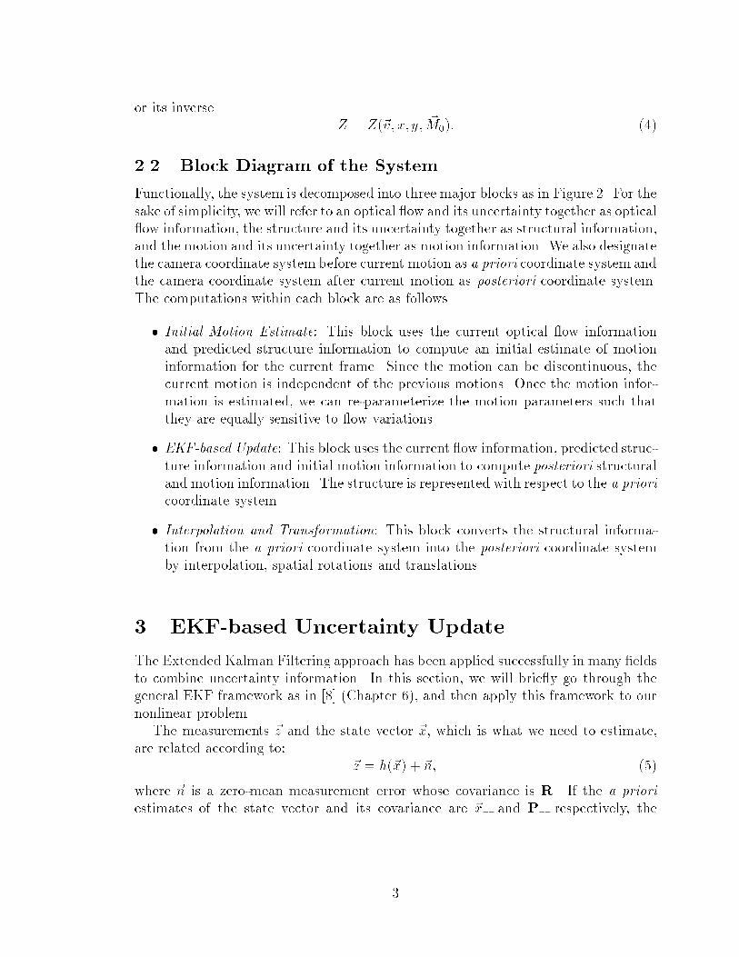
Figure 1: The Camera Coordinate

other mathematical techniques such as Sherman-Morrison-Woodbury inversionand principal component analysis, we can achieve an O(N) numerical algorithmto compute Kalman �ltering.

� The underlying motion of the camera can be discontinuous. Unlike many EKF-based approaches, ours computes the initial motion of every frame independently.

� We propose the concept of \Dynamic Motion Parameterization", which meansthat a di�erent parameterization of the six motion parameters is used at everyframe. Such a dynamic parameterization enables that the optical ow is equallysensitive to each of them, and therefore, stabilizes numerical computations.

2 System Overview

2.1 Coordinates and Motion

The system is based on the camera coordinate system OXY Z shown in Figure 1, inwhich the origin O is the center of projection, the Z axis coincides with the opticalaxis, and the image plane is located at Z = 1.

If the relative motion of the camera with respect to the scene is composed of atranslation velocity (U;V;W ) and a rotation velocity (A;B;C), we have the followingrelation between the ow velocity (vx; vy) and the depth Z of pixel location (x; y)from [14]:

vx =�U + xW

Z+Axy �B(x2 + 1) + Cy; (1)

vy =�V + yW

Z�Bxy +A(y2 + 1) � Cx: (2)

If we designate the camera motion parameterization as ~M0 = (U;V;W;A;B;C)T andthe ow velocity as ~v = (vx; vy)T , the above equation can be expressed as

~v = ~v(x; y; Z; ~M0); (3)

2

or its inverseZ = Z(~v; x; y; ~M0): (4)

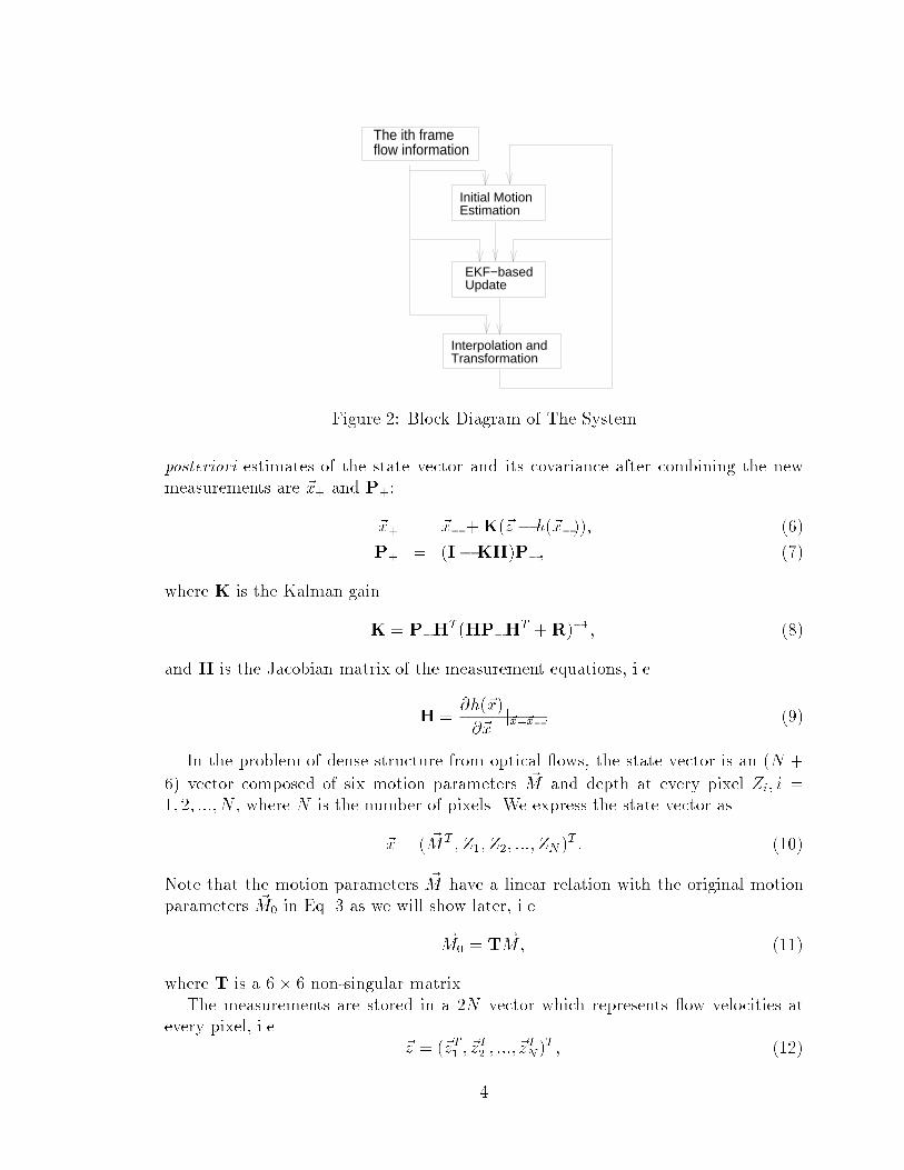
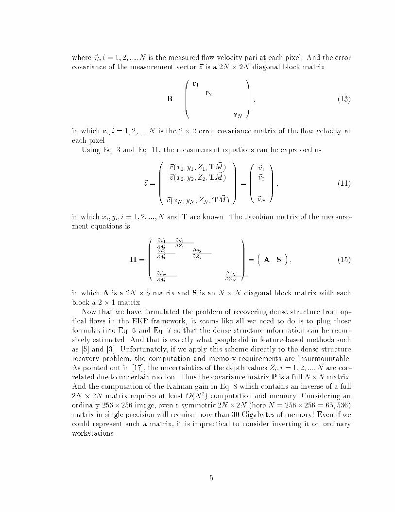
2.2 Block Diagram of the System

Functionally, the system is decomposed into three major blocks as in Figure 2. For thesake of simplicity, we will refer to an optical ow and its uncertainty together as optical ow information, the structure and its uncertainty together as structural information,and the motion and its uncertainty together as motion information. We also designatethe camera coordinate system before current motion as a priori coordinate system andthe camera coordinate system after current motion as posteriori coordinate system.The computations within each block are as follows.

� Initial Motion Estimate: This block uses the current optical ow informationand predicted structure information to compute an initial estimate of motioninformation for the current frame. Since the motion can be discontinuous, thecurrent motion is independent of the previous motions. Once the motion infor-mation is estimated, we can re-parameterize the motion parameters such thatthey are equally sensitive to ow variations.

� EKF-based Update: This block uses the current ow information, predicted struc-ture information and initial motion information to compute posteriori structuraland motion information. The structure is represented with respect to the a prioricoordinate system.

� Interpolation and Transformation: This block converts the structural informa-tion from the a priori coordinate system into the posteriori coordinate systemby interpolation, spatial rotations and translations.

3 EKF-based Uncertainty Update

The Extended Kalman Filtering approach has been applied successfully in many �eldsto combine uncertainty information. In this section, we will brie y go through thegeneral EKF framework as in [8] (Chapter 6), and then apply this framework to ournonlinear problem.

The measurements ~z and the state vector ~x, which is what we need to estimate,are related according to:

~z = h(~x) + ~n; (5)

where ~n is a zero-mean measurement error whose covariance is R. If the a priori

estimates of the state vector and its covariance are ~x� and P� respectively, the

3

Initial MotionEstimation

EKF−basedUpdate

Interpolation andTransformation

The ith frameflow information

Figure 2: Block Diagram of The System

posteriori estimates of the state vector and its covariance after combining the newmeasurements are ~x+ and P+:

~x+ = ~x� +K(~z � h(~x�)); (6)

P+ = (I�KH)P�; (7)

where K is the Kalman gain

K = P�HT (HP�H

T +R)�1; (8)

and H is the Jacobian matrix of the measurement equations, i.e.

H =@h(~x)

@~xj~x=~x

�

: (9)

In the problem of dense structure from optical ows, the state vector is an (N +

6) vector composed of six motion parameters ~M and depth at every pixel Zi; i =1; 2; :::;N , where N is the number of pixels. We express the state vector as

~x = ( ~MT ; Z1; Z2; :::;ZN )T : (10)

Note that the motion parameters ~M have a linear relation with the original motionparameters ~M0 in Eq. 3 as we will show later, i.e.

~M0 = T ~M; (11)

where T is a 6� 6 non-singular matrix.The measurements are stored in a 2N vector which represents ow velocities at

every pixel, i.e.~z = (~zT1 ; ~z

T2 ; :::; ~z

TN)

T ; (12)

4

where ~zi; i = 1; 2; :::;N is the measured ow velocity pari at each pixel. And the errorcovariance of the measurement vector ~z is a 2N � 2N diagonal block matrix

R =

0BBBB@r1

r2. . .

rN

1CCCCA ; (13)

in which ri; i = 1; 2; :::;N is the 2 � 2 error covariance matrix of the ow velocity ateach pixel.

Using Eq. 3 and Eq. 11, the measurement equations can be expressed as

~z =

0BBBBB@

~v(x1; y1;Z1;T ~M )

~v(x2; y2;Z2;T ~M )...

~v(xN ; yN ;ZN ;T ~M )

1CCCCCA =

0BBBB@

~v1~v2...~vN

1CCCCA ; (14)

in which xi; yi; i = 1; 2; :::;N and T are known. The Jacobian matrix of the measure-ment equations is

H =

0BBBBB@

@~v1@ ~M

@~v1@Z1

@~v2@ ~M

@~v2@Z2

.... . .

@~vN@ ~M

@~vN@ZN

1CCCCCA =

�A S

�; (15)

in which A is a 2N � 6 matrix and S is an N � N diagonal block matrix with eachblock a 2 � 1 matrix.

Now that we have formulated the problem of recovering dense structure from op-tical ows in the EKF framework, it seems like all we need to do is to plug thoseformulas into Eq. 6 and Eq. 7 so that the dense structure information can be recur-sively estimated. And that is exactly what people did in feature-based methods suchas [5] and [3]. Unfortunately, if we apply this scheme directly to the dense structurerecovery problem, the computation and memory requirements are insurmountable.As pointed out in [17], the uncertainties of the depth values Zi; i = 1; 2; :::;N are cor-related due to uncertain motion. Thus the covariance matrixP is a fullN�N matrix.And the computation of the Kalman gain in Eq. 8 which contains an inverse of a full2N � 2N matrix requires at least O(N2) computation and memory. Considering anordinary 256�256 image, even a symmetric 2N �2N (here N = 256�256 = 65; 536)matrix in single precision will require more than 30 Gigabytes of memory! Even if wecould represent such a matrix, it is impractical to consider inverting it on ordinaryworkstations.

5

3.1 Decomposition of Independent and Correlated Uncer-

tainty

Fortunately, we can take advantage of this speci�c problem to overcome these di�cul-ties. As we mentioned before, the uncertainties of the depth values are correlated dueto uncertain motion. Because there are only six motion parameters, the correlateduncertainty of the depth values caused by a single uncertain motion is an N � N

matrix with rank of only six!Because the rank of the correlated uncertainty is much smaller than N , the co-

variance matrix P can be decomposed into the following format:

P =

Cm CT

p

Cp (Cs +UVT )

!; (16)

where Cm is a 6�6 matrix representing the covariance of the motion parameters, Cp

is an N�6 matrix representing the correlation between the motion and the structure,Cs is an N�N diagonal matrix representing the independent uncertainty of the depthvalue of each pixel, and U and V are both N � k matrices whose outer product is arank k matrix representing the correlated uncertainty of the depth values. Therefore,storing the matrix P sparsely will only require O(N) memory if k is a constant.

Now that we can represent the covariance matrix P, we will show that in theEKF framework, once P� can be represented in the format of Eq. 16, P+ can alsobe represented in the same format. In fact, because R and H are special matrices,the covariance matrix P can always be represented sparsely as in Eq. 16 throughoutthe whole optical ow sequence. We never need to explicitly represent P as an(N + 6) � (N + 6) matrix!

In our system, we assume that the motion is discontinuous, i.e. the current motionis uncorrelated to previous motions. Under this assumption, a priori correlationbetween the structure and the current motion Cp in Eq. 16 is zero. For simplicity,we will assume Cp is zero in the following sections, though in situations where thisassumption is not true we also have similar results. If P� is represented as in Eq. 16,after some manipulation, we have

HP�HT +R = (SCsS

T +R) +

0B@ ACm SU

1CA

AT

VTST

!

= C1 +U1VT1 ; (17)

where C1 = (SCsST +R) is an N �N diagonal block matrix with each block a 2� 2

matrix, U1 and V1 are 2N � (k + 6) matrices as

U1 =

0B@ ACm SU

1CA ;V1 =

0B@ A SV

1CA : (18)

6

By applying the Sherman-Morrison-Woodbury formula as in [9] and Appendix A,we can invert the above matrix

(HP�HT +R)�1 = (C1 +U1V

T1 )

�1 = C2 +U2VT2 ; (19)

where C2 is also an N �N diagonal block matrix with each block a 2� 2 matrix, U2

and V1 are 2N � (k + 6) matrices.Substituting Eq. 19 back into Eq. 8, we obtain the Kalman gain

K =

Km

C3 +U3VT3

!; (20)

where Km is a 6� 2N matrix

Km = CmATC2 +CmA

TU2VT2 ; (21)

C3 is an N �N diagonal block matrix with each block a 1 � 2 matrix

C3 = CsSTC2; (22)

U3 is a (N + 6)� (3k + 6) matrix

U3 =

0B@ U CsS

TU2 U

1CA ; (23)

and V3 is a 2N � (3k + 6) matrix

V3 =

0B@ C2SV V2 V2(UT

2 SV)

1CA : (24)

Finally, the updated covariance P+ is

P+ =

Cmp CT

pp

Cpp (C4 +U4VT4)

!; (25)

where Cmp is a 6 � 6 posteriori covariance matrix of the motion parameters

Cmp = Cm �KmACm; (26)

Cpp is an N � 6 posteriori uncertainty correlation between the structure and currentmotion1

Cpp = �(Cs +UVT )STKTm; (27)

1Note that we assumed a priori correlation between structure and motion Cp is zero. But the

posteriori correlation Cpp is not zero.

7

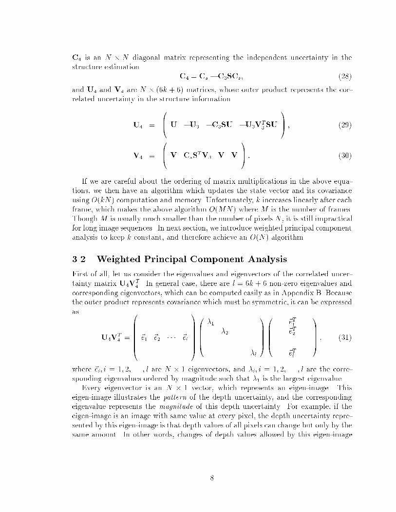
C4 is an N � N diagonal matrix representing the independent uncertainty in thestructure estimation

C4 = Cs �C3SCs; (28)

and U4 and V4 are N � (6k + 6) matrices, whose outer product represents the cor-related uncertainty in the structure information

U4 =

0B@ U �U3 �C3SU �U3V

T3SU

1CA ; (29)

V4 =

0B@ V CsS

TV3 V V

1CA : (30)

If we are careful about the ordering of matrix multiplications in the above equa-tions, we then have an algorithm which updates the state vector and its covarianceusing O(kN) computation and memory. Unfortunately, k increases linearly after eachframe, which makes the above algorithm O(MN) where M is the number of frames.Though M is usually much smaller than the number of pixels N , it is still impracticalfor long image sequences. In next section, we introduce weighted principal componentanalysis to keep k constant, and therefore achieve an O(N) algorithm.

3.2 Weighted Principal Component Analysis

First of all, let us consider the eigenvalues and eigenvectors of the correlated uncer-tainty matrix U4V

T4. In general case, there are l = 6k + 6 non-zero eigenvalues and

corresponding eigenvectors, which can be computed easily as in Appendix B. Becausethe outer product represents covariance which must be symmetric, it can be expressedas

U4VT4 =

0BBBBBB@~e1 ~e2 � � � ~el

1CCCCCCA

0BBBB@�1

�2. . .

�l

1CCCCA

0BBBB@

~eT1~eT2...~eTl

1CCCCA ; (31)

where ~ei; i = 1; 2; . . . ; l are N � 1 eigenvectors, and �i; i = 1; 2; . . . ; l are the corre-sponding eigenvalues ordered by magnitude such that �1 is the largest eigenvalue.

Every eigenvector is an N � 1 vector, which represents an eigen-image. Thiseigen-image illustrates the pattern of the depth uncertainty, and the correspondingeigenvalue represents the magnitude of this depth uncertainty. For example, if theeigen-image is an image with same value at every pixel, the depth uncertainty repre-sented by this eigen-image is that depth values of all pixels can change but only by thesame amount. In other words, changes of depth values allowed by this eigen-image

8

have to be in the pattern speci�ed by the eigen-image:

�

0BBBB@

Z1

Z2

...ZN

1CCCCA = c~e; (32)

where c is a scalar constant and ~e is the eigen-image. The meaning of the eigenvalueis similar to that of � in a Gaussian distribution, which represents the magnitude ofthe uncertainty.

Since the eigenvalues in Eq. 31 are in descending order, and we can truncate theeigenvalues after �rst k largest ones, i.e.

U4VT4 �

0BBBBBB@~e1 ~e2 � � � ~ek

1CCCCCCA

0BBBB@

�1�2

. . .

�k

1CCCCA

0BBBB@

~eT1

~eT2...~eTk

1CCCCA : (33)

Thus U4 and V4 can both be reduced to N � k matrices. The iterations of EKFupdating illustrated in the previous section can be carried out in O(N) for everyframe no matter how long the sequence is.

The underlying assumption of truncating small eigenvalues in Eq. 33 is that theuncertainty implied by those eigenvalues/eigen-images is negligible compared to theindependent uncertainty C4. And the reason for keeping large eigenvalues is that weassume the uncertainties implied by these large eigenvalues and their correspondingeigenvectors are at least comparable to the independent uncertainty C4. But sincethe independent uncertainties of pixels are not uniform, truncating by the magni-tudes of eigenvalues may not make much sense at all because even though a rela-tively large eigenvalue may imply a large uncertainty in a certain area in the eigen-image, if the independent uncertainty happens to be even larger in the same area,this eigenvalue/eigen-image becomes less signi�cant.

Based on the above speculation, we propose a weighted principal component anal-ysis, i.e. the correlated uncertainty is weighted by independent uncertainty beforedecomposition as in Eq. 31. Since the independent uncertainty C4 is a diagonalmatrix, and its diagonal elements have to be positive, we can decompose it as

C4 =

0BBBB@

c1c2

. . .

cN

1CCCCA

=

0BBBB@

pc1 p

c2. . . p

cN

1CCCCA

0BBBB@

pc1 p

c2. . . p

cN

1CCCCA = QQT : (34)

9

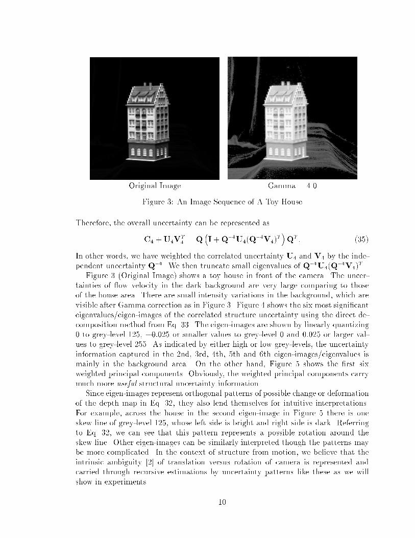
Original Image Gamma = 4.0

Figure 3: An Image Sequence of A Toy House

Therefore, the overall uncertainty can be represented as

C4 +U4VT4= Q

�I+Q�1U4(Q

�1V4)T�QT : (35)

In other words, we have weighted the correlated uncertainty U4 and V4 by the inde-pendent uncertainty Q�1. We then truncate small eigenvalues of Q�1U4(Q�1V4)T .

Figure 3 (Original Image) shows a toy house in front of the camera. The uncer-tainties of ow velocity in the dark background are very large comparing to thoseof the house area. There are small intensity variations in the background, which arevisible after Gamma correction as in Figure 3. Figure 4 shows the six most signi�canteigenvalues/eigen-images of the correlated structure uncertainty using the direct de-composition method from Eq. 33. The eigen-images are shown by linearly quantizing0 to grey-level 125, �0:025 or smaller values to grey-level 0 and 0:025 or larger val-ues to grey-level 255. As indicated by either high or low grey-levels, the uncertaintyinformation captured in the 2nd, 3rd, 4th, 5th and 6th eigen-images/eigenvalues ismainly in the background area. On the other hand, Figure 5 shows the �rst sixweighted principal components. Obviously, the weighted principal components carrymuch more useful structural uncertainty information.

Since eigen-images represent orthogonal patterns of possible change or deformationof the depth map in Eq. 32, they also lend themselves for intuitive interpretations.For example, across the house in the second eigen-image in Figure 5 there is oneskew line of grey-level 125, whose left side is bright and right side is dark. Referringto Eq. 32, we can see that this pattern represents a possible rotation around theskew line. Other eigen-images can be similarly interpreted though the patterns maybe more complicated. In the context of structure from motion, we believe that theintrinsic ambiguity [2] of translation versus rotation of camera is represented andcarried through recursive estimations by uncertainty patterns like these as we willshow in experiments.

10

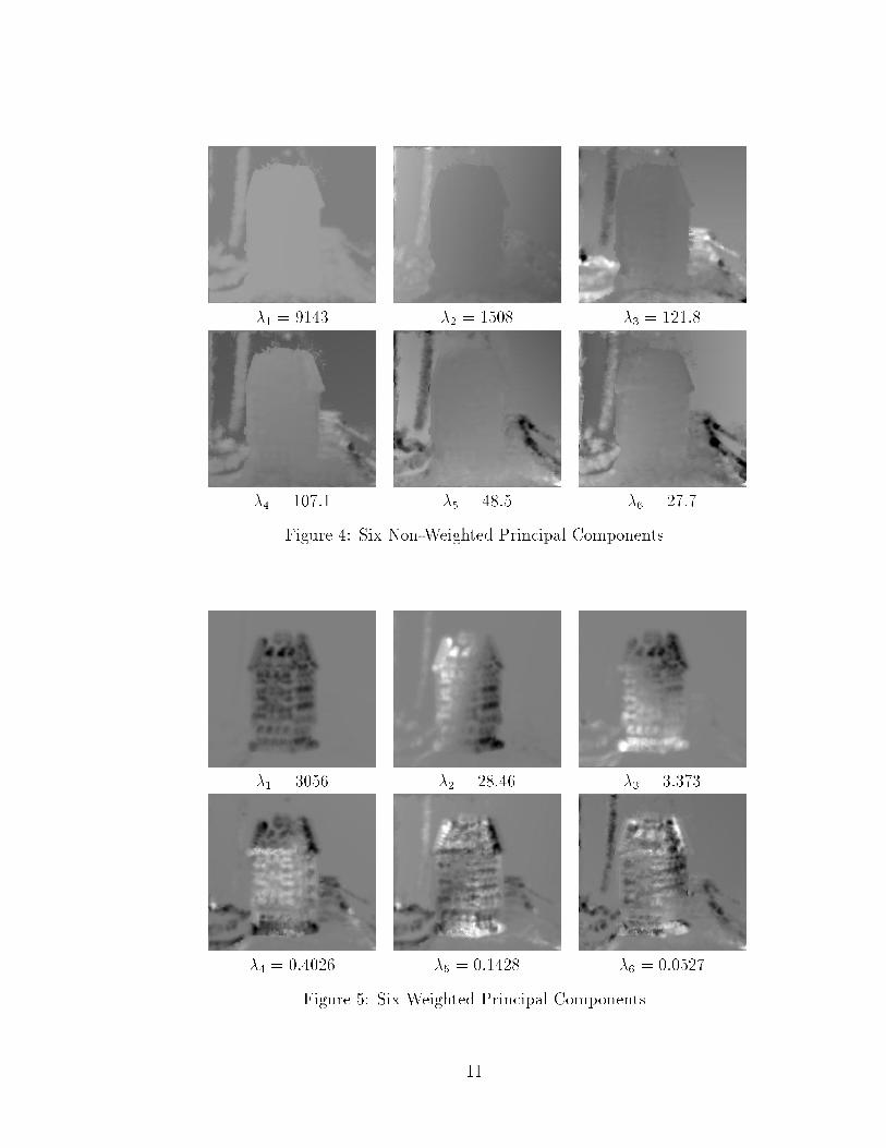
�1 = 9143 �2 = 1508 �3 = 121:8

�4 = 107:1 �5 = 48:5 �6 = 27:7

Figure 4: Six Non-Weighted Principal Components

�1 = 3056 �2 = 28:46 �3 = 3:373

�4 = 0:4026 �5 = 0:1428 �6 = 0:0527

Figure 5: Six Weighted Principal Components

11

4 Initial Motion Estimation

Unlike many other approaches such as [3], we do not assume continuous motion. Inother words, we assume that the motion at the current frame is totally unrelatedto the motion in the previous frame because we believe that the continuous motionassumption is unrealistic in many cases such as navigating on real roads, hand-heldvideo recording, and so on. Thus, in order to apply the EKF framework to our prob-lem, we need to estimate an initial motion and its a priori covariance for each frame.Theoretically we don't need a priori covariance because it should be in�nitely large.But in practice we need a �nite one for numerical stability and re-parameterization.

First of all, given a priori structure Z and ow velocity v, we can estimate theinitial motion ~M0 from Eq. 3 by a linear least squares �tting, e.g. minimizing

NXi=1

(~vi � ~v(xi; yi; Zi; ~M0))T r�1i (~vi � ~v(xi; yi; Zi; ~M0)); (36)

where ri is the covariance of the ow velocity ~vi.But we cannot use the above minimization to estimate the covariance of ~M0 because

we didn't consider the uncertainties of structure Z. Designating the a priori depthmap as ~Za and the depth computed from current motion M0 and ~v by Eq. 4 as ~Zc,we have the following objective function to be minimized

NXi=1

(~vi � ~v(xi; yi; Zi; ~M0))T r�1

i (~vi � ~v(xi; yi; Zi; ~M0)) +

(~Za � ~Zc)T (C+Cd +UVT )�1(~Za � ~Zc); (37)

where ~Za and ~Zc are N �1 vectors, C+UVT is the structural uncertainty of ~Za, andCd is the depth uncertainty caused by current ow uncertainty given ~M0. Becausethe ow uncertainties of di�erent pixels are independent, Cd is an N � N diagonalmatrix.

If we ignore the dependence of Cd on ~M0, the minimization of Eq. 37 can beachieved using Levenberg-Marquardt method [16]. In fact, this simpli�cation is jus-

ti�able because Cd is usually insensitive to ~M0. Once the objective function is mini-mized, the curvature at the minimal value can be used to compute the covariance of~M0.

4.1 Dynamic Motion Parameterization

Motion is traditionally parameterized using three translation parameters and threerotation parameters as in Eq. 1 and Eq. 2. As pointed out in [3], if the camera hasa long focal length, the optical ow is much more sensitive to translations in the XYplane to translations in the Z direction. Ideally we want the optical ow to be equallysensitive to all six motion parameters because otherwise the the covariance of motion

12

Cm in EQ. 16 could be numerically singular or near singular and therefore ruin thenumerical computation of EKF.

We introduce the concept of \dynamic motion parameterization" to equalize sen-sitivities of motion parameters. There are two sources of sensitivity di�erence:

1. Static Sensitivity Di�erence is caused by the camera con�guration. For example,if the camera has a narrow �eld of view, the optical ow is usually much moresensitive to rotation than translation.

2. Dynamic Sensitivity Di�erence is caused by current ow or depth estimate in-stead of the camera. For example, if the optical ow has uncertainty much largerin one direction than others, the optical ow is less sensitive to the motion whichcaused optical ow in that direction.

If we designate the covariance of ~M0 computed from minimizing the objectivefunction of Eq. 37 as Cmt, we can normalize sensitivities by using a new set of motionparameters

~M = T�1 ~M0; (38)

whereCmt = TTT : (39)

It can be easily veri�ed that the covariance of the new motion vector ~M is the unitmatrix I.

Note that we cannot use the unit matrix as Cm in Eq. 16. Theoretically the a

priorimotion covariance Cm should be in�nitely large due to uncorrelated motion. Inestimating covariance of the motion in this section, we have already used the optical ow information of the current frame. Therefore, it is actually posteriori motioncovariance! Ideally, we want the a priori covariances to be small enough to avoidnumerical problems, and yet large enough to not contain any information about thecurrent frame. In practice, we use 1000I as a priori motion covariance Cm because itavoids the numerical problem of an in�nitely large covariance and is also large enough(compared to posteriori covariance I) to be uninformative.

5 Interpolation and Forward Transformation

We represent the 3D shape by a depth map in the current camera coordinate systemas in Figure 1. Therefore, we need to transform the previous depth map into thecurrent camera coordinate system and resample the depth map according to thecurrent sensor grid. There are two new problems which were previously unsolved:

� Though the depth map and its independent uncertainty can be easily interpo-lated as in [15, 12], the interpolation of correlated uncertainty is a new problem.

� Most existing recursive structure-from-motion systems ignore the fact that mo-tion and structure are actually correlated as Cpp in Eq. 25 when they rotate or

13

Row

Colume

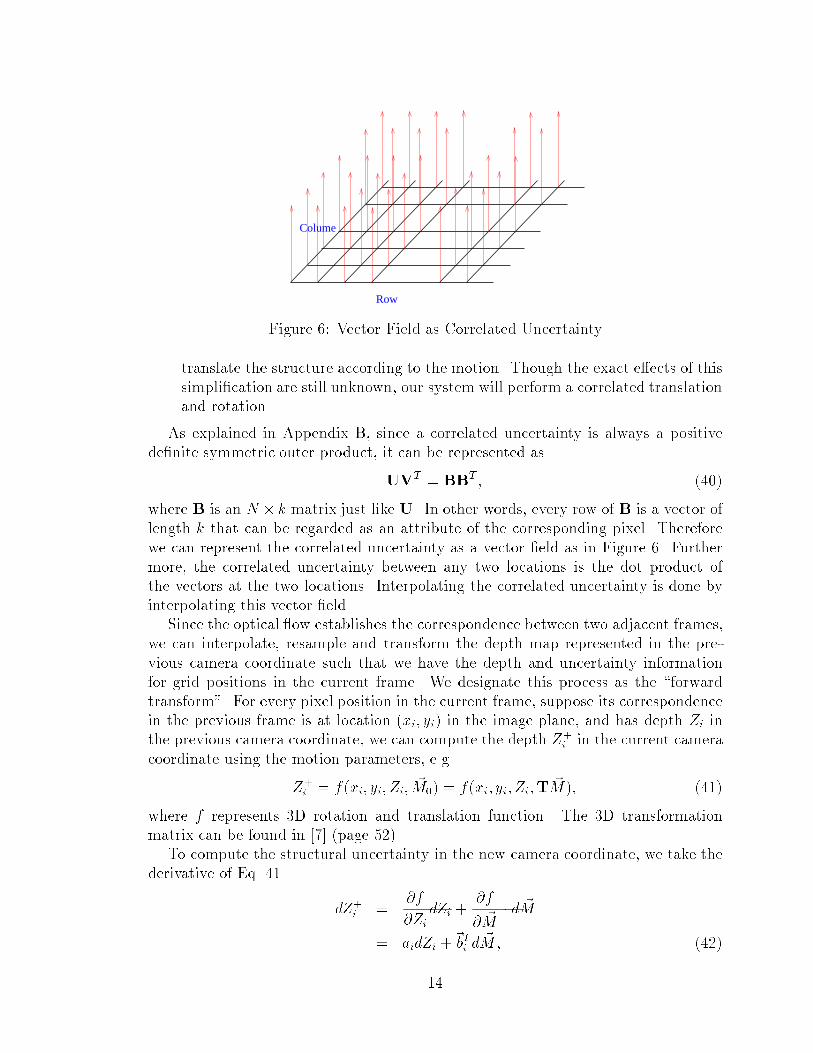
Figure 6: Vector Field as Correlated Uncertainty

translate the structure according to the motion. Though the exact e�ects of thissimpli�cation are still unknown, our system will perform a correlated translationand rotation.

As explained in Appendix B, since a correlated uncertainty is always a positivede�nite symmetric outer product, it can be represented as

UVT = BBT ; (40)

where B is an N � k matrix just like U. In other words, every row of B is a vector oflength k that can be regarded as an attribute of the corresponding pixel. Thereforewe can represent the correlated uncertainty as a vector �eld as in Figure 6. Furthermore, the correlated uncertainty between any two locations is the dot product ofthe vectors at the two locations. Interpolating the correlated uncertainty is done byinterpolating this vector �eld.

Since the optical ow establishes the correspondence between two adjacent frames,we can interpolate, resample and transform the depth map represented in the pre-vious camera coordinate such that we have the depth and uncertainty informationfor grid positions in the current frame. We designate this process as the \forwardtransform". For every pixel position in the current frame, suppose its correspondencein the previous frame is at location (xi; yi) in the image plane, and has depth Zi inthe previous camera coordinate, we can compute the depth Z+

i in the current cameracoordinate using the motion parameters, e.g.

Z+

i = f (xi; yi; Zi; ~M0) = f(xi; yi;Zi;T ~M); (41)

where f represents 3D rotation and translation function. The 3D transformationmatrix can be found in [7] (page 52).

To compute the structural uncertainty in the new camera coordinate, we take thederivative of Eq. 41

dZ+

i =@f

@Zi

dZi +@f

@ ~M� d ~M

= aidZi +~bTi d~M; (42)

14

where ~bi is a vector of length six. Thus we have the covariance between two arbitrarypoints as

E[dZ+

i dZ+

j ] = aiajE[dZidZj ] + ai~bTj E[dZid ~M ] +

aj~bTi E[dZjd ~M ] +~bTi E[d ~Md ~MT ]~bj: (43)

From Eq. 25, we know that

Cmp = E[d ~Md ~MT ]; (44)

Cpp =

0BBBBB@

E[dZ1d ~M ]T

E[dZ2d ~M ]T

...

E[dZNd ~M ]T

1CCCCCA : (45)

Therefore, we have the structural uncertainty after the forward transform as

E

2666664

0BBBB@dZ+

1

dZ+

2

...dZ+

N

1CCCCA

0BBBB@dZ+

1

dZ+

2

...dZ+

N

1CCCCA

T3777775 = C+ +U+(V+)T ; (46)

where

C+ =

0BBB@a21

a22

� � �a2N

1CCCAC4; (47)

U+ =

0BBBBB@

a1~uT1 a1~p

T1

~bT1 Cmp~bT1

a2~uT2 a2~p

T2

~bT2 Cmp~bT2

......

......

aN~uTN aN~p

TN

~bTN Cmp~bTN

1CCCCCA ; (48)

V+ =

0BBBBB@

a1~vT1

~bT1 a1~pT1

~bT1a2~v

T2

~bT2 a2~pT2

~bT2...

......

...

aN~vTN

~bTN aN~pTN

~bTN

1CCCCCA ; (49)

where

U4 =

0BBBB@

~uT1~uT2

...~uTN

1CCCCA ; (50)

15

V4 =

0BBBB@~vT1~vT2

...~vTN

1CCCCA ; (51)

Cpp =

0BBBB@

~pT1

~pT2...~pTN

1CCCCA ; (52)

in which ~ui's and ~vi's are vectors of length k and ~pk's are of length six. Since U+ andV+ are now N � (k + 18) matrices, they may also be reduced to N � k by weightedprincipal component analysis.

6 Implementation Issues and Experiments

6.1 Implementation Issues

We implemented our system using single precision matrices. As always in manipulat-ing large matrices, the numerical stability has to be carefully watched while carryingout those computations. Potentially there are following sources of unstable compu-tations:

1. Matrix Multiplication: When computing the inner product of two large matrixVTU, where both U and V are N � k (k << N ), we have to carry thoseadditions in double precision due to large N . For example, if the image is256�256, we can easily lose four signi�cant digits during multiplications, whichcould be devastating if they are carried out in only single precision.

2. Ill-conditioned Matrix: There is always a danger when one of the matrices inthe computation is singular or near singular. In the worst case, we may lose allsigni�cant digits. Thus it is extremely helpful to avoid any ill-conditioned matrixif possible. In our system, we pay special attention to the following matrices:

� Flow Uncertainty: The estimated optical ow uncertainty ri's in Eq. 13.

� Motion Uncertainty: We used dynamic motion parameterization to preventthe motion covariance matrix from being ill-conditioned.

� Kalman Gain: In computing the Kalman gain as in Eq. 8, it is numeri-cally devastating if HP�H

T +R is ill-conditioned. HP�HT represents the

projection of the uncertainty of motion and structure to the uncertainty ofoptical ow. In order for HP�H

T + R to be well conditioned, we need tomake sure that the projected uncertainty of optical ow is not signi�cantlylarger (> 105) than the estimated uncertainty R. That is the reason wechoose 1000I as the a priori motion uncertainty.

16

3. Sherman-Morrison-Woodbury Inversion: Though Sherman-Morrison-Woodburyinversion signi�cantly reduces the amount of computation and memory requiredcompared to the traditional Gaussian elimination ([16]), it has the disadvantageof being more fragile numerically ([10, 4], Appendix A). From our experience,the eigenvalues of UVT have to be at most 104 of the eigenvalues of C to allowa stable numerical inversion of C + UVT using Sherman-Morrison-Woodburyformula.

Another common problem of a structure from motion system is the handling ofthe disappearance and reappearance of parts of the scene due to relative movementbetween the camera and the scene. Our system had no problem dealing with newparts, which are simply assigned a preset large independent uncertainty and a zerocorrelated uncertainty. But the depth information of disappearing parts is discarded.In the future, we would like to maintain a global shape module such that the structureinformation of disappeared parts could be stored and retrieved.

6.2 Experiments

We tested our system on real image sequences taken by a Sony XC-75 video cam-era. The relative camera movements in all the sequences involve both rotation andtranslation. We digitized images in two ways. One is to digitize by matrox boardwhile shooting the sequence. In order to digitize while taking images, we mount thecamera on a computer-controlled 6 DOF platform in Calibrated Imaging Lab, andstop for every frame. Another way is to record the sequence on Umatic SP video tape,and digitize the tape frame by frame. Unfortunately, the digitizing device we havecan only digitize one of two �elds in every frame, and the videotape also introducesadditional noise in the images. We will demonstrate the performance of our systemon image sequences digitized both ways. All images in our experiments are 480�512.

6.2.1 Ambiguities

It is well known that there are intrinsic ambiguities in recovering structure frommotion. The �rst kind of ambiguity, i.e. the scale ambiguity, states that the scale ofthe object or the absolute depth of the object can never be recovered. Secondly, if thecamera has a small �eld of view, the optical ow caused by a small camera rotation isvery similar to that caused by a small camera translation. Therefore, given an optical ow, there is a rotation/translation ambiguity. Thirdly, since the optical ow has itsuncertainty, we will always have uncertainty in estimating other motion parameterssuch as rotation and translation around z axis though they are usually less signi�cant.We also like to point out that there is no fundamental di�erence in terms of originbetween the second and the third kinds of ambiguities other than their magnitudesfor an ordinary camera. Historically the second kind of ambiguity was frequentlysingled out in literature.

In our system, we assign an initial depth and uncertainty to the �rst frame. Prac-tically we assign a at depth map and uniform independent uncertainty as a priori

17

depth information. It serves two purposes, which are disambiguation of the scale am-biguity by providing absolute depth, and allowing deformation of the a priori depthmap to the true depth map by providing large independent uncertainty.

Our system keeps six principal eigenimages to represent the correlated uncertaintyas shown in Figure 5. Among these eigenimages, the �rst one usually represents the�rst kind of ambiguity, i.e. the scale ambiguity. The second and the third ones usuallyrepresent the second kind of ambiguity in two orthogonal directions. And the restones represent other minor ambiguities.

Conceptually the independent uncertainty represents a chaotic uncertainty pat-tern, while the correlated uncertainty represents an organized uncertainty pattern.For example, if the eigenimage of a correlated uncertainty is uniformly bright, it rep-resents that the corresponding depth map can move back and forth. In other words,the depth values of all pixels have to change uniformly while the shape doesn't changeat all. Since we set a priori depth uncertainty as totally chaotic, we will expect thatas more optical ow information is incorporated, the uncertainty will become less andless chaotic, more and more organized. In our framework, that means that magnitudeof the independent uncertainty will decrease while the magnitude of the correlateduncertainty could increase.

Optical ow information doesn't provide anything which we could use to eliminatethe scale ambiguity. Therefore we expect the eigenimage representing scale ambiguityin correlated uncertainty will have larger and larger eigenvalue. On the other hands,the second and third kinds of ambiguities are strong in some optical ows whileweak in other ones. Thus the eigenimages representing these ambiguities can haveincreasing or decreasing eigenvalues depending on the optical ow sequence.

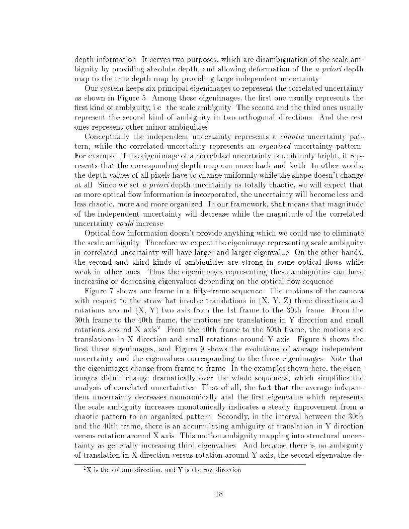
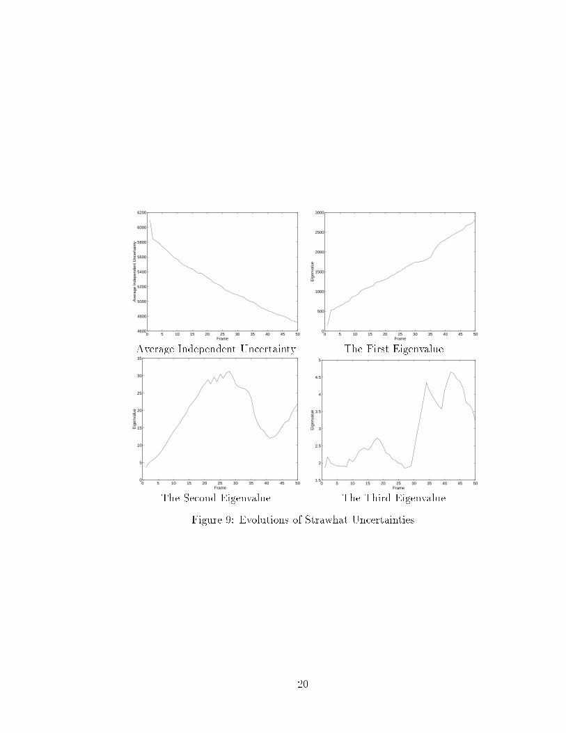
Figure 7 shows one frame in a �fty-frame sequence. The motions of the camerawith respect to the straw hat involve translations in (X, Y, Z) three directions androtations around (X, Y) two axis from the 1st frame to the 30th frame. From the30th frame to the 40th frame, the motions are translations in Y direction and smallrotations around X axis2. From the 40th frame to the 50th frame, the motions aretranslations in X direction and small rotations around Y axis. Figure 8 shows the�rst three eigenimages, and Figure 9 shows the evolutions of average independentuncertainty and the eigenvalues corresponding to the three eigenimages. Note thatthe eigenimages change from frame to frame. In the examples shown here, the eigen-images didn't change dramatically over the whole sequences, which simpli�es theanalysis of correlated uncertainties. First of all, the fact that the average indepen-dent uncertainty decreases monotonically and the �rst eigenvalue which representsthe scale ambiguity increases monotonically indicates a steady improvement from achaotic pattern to an organized pattern. Secondly, in the interval between the 30thand the 40th frame, there is an accumulating ambiguity of translation in Y directionversus rotation around X axis. This motion ambiguity mapping into structural uncer-tainty as generally increasing third eigenvalues. And because there is no ambiguityof translation in X direction versus rotation around Y axis, the second eigenvalue de-

2X is the column direction, and Y is the row direction

18

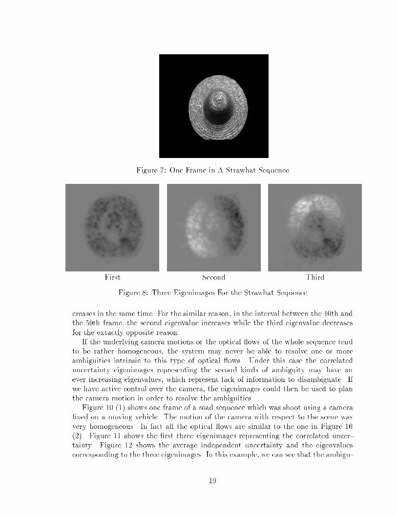
Figure 7: One Frame in A Strawhat Sequence

First Second Third

Figure 8: Three Eigenimages For the Strawhat Sequence

creases in the same time. For the similar reason, in the interval between the 40th andthe 50th frame, the second eigenvalue increases while the third eigenvalue decreasesfor the extactly opposite reason.

If the underlying camera motions or the optical ows of the whole sequence tendto be rather homogeneous, the system may never be able to resolve one or moreambiguities intrinsic to this type of optical ows. Under this case the correlateduncertainty eigenimages representing the second kinds of ambiguity may have anever increasing eigenvalues, which represent lack of information to disambiguate. Ifwe have active control over the camera, the eigenimages could then be used to planthe camera motion in order to resolve the ambiguities.

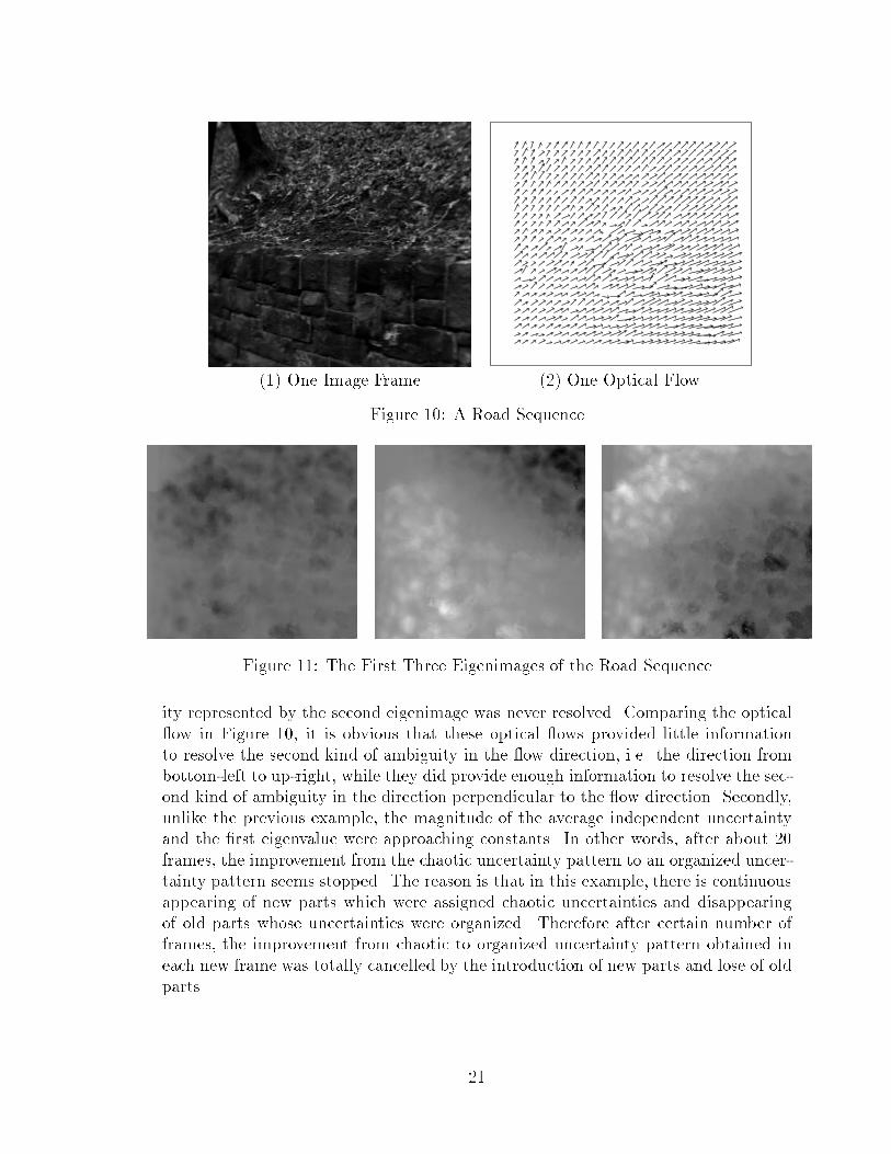
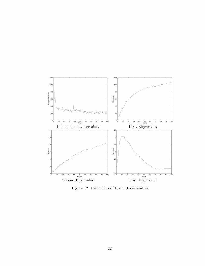
Figure 10 (1) shows one frame of a road sequence which was shoot using a camera�xed on a moving vehicle. The motion of the camera with respect to the scene wasvery homogeneous. In fact all the optical ows are similar to the one in Figure 10(2). Figure 11 shows the �rst three eigenimages representing the correlated uncer-tainty. Figure 12 shows the average independent uncertainty and the eigenvaluescorresponding to the three eigenimages. In this example, we can see that the ambigu-

19

0 5 10 15 20 25 30 35 40 45 504600

4800

5000

5200

5400

5600

5800

6000

6200

Frame

Ave

rage

Inde

pend

ent U

ncer

tain

ty

0 5 10 15 20 25 30 35 40 45 500

500

1000

1500

2000

2500

3000

Frame

Eig

enva

lue

Average Independent Uncertainty The First Eigenvalue

0 5 10 15 20 25 30 35 40 45 500

5

10

15

20

25

30

35

Frame

Eig

enva

lue

0 5 10 15 20 25 30 35 40 45 501.5

2

2.5

3

3.5

4

4.5

5

Frame

Eig

enva

lue

The Second Eigenvalue The Third Eigenvalue

Figure 9: Evolutions of Strawhat Uncertainties

20

(1) One Image Frame (2) One Optical Flow

Figure 10: A Road Sequence

Figure 11: The First Three Eigenimages of the Road Sequence

ity represented by the second eigenimage was never resolved. Comparing the optical ow in Figure 10, it is obvious that these optical ows provided little informationto resolve the second kind of ambiguity in the ow direction, i.e. the direction frombottom-left to up-right, while they did provide enough information to resolve the sec-ond kind of ambiguity in the direction perpendicular to the ow direction. Secondly,unlike the previous example, the magnitude of the average independent uncertaintyand the �rst eigenvalue were approaching constants. In other words, after about 20frames, the improvement from the chaotic uncertainty pattern to an organized uncer-tainty pattern seems stopped. The reason is that in this example, there is continuousappearing of new parts which were assigned chaotic uncertainties and disappearingof old parts whose uncertainties were organized. Therefore after certain number offrames, the improvement from chaotic to organized uncertainty pattern obtained ineach new frame was totally cancelled by the introduction of new parts and lose of oldparts.

21

0 10 20 30 40 50 60 70 80 90 1000

500

1000

1500

2000

2500

3000

Frame

Ave

rage

Unc

erta

inty

0 10 20 30 40 50 60 70 80 90 1000

200

400

600

800

1000

1200

Frame

Eig

enva

lue

Independent Uncertainty First Eigenvalue

0 10 20 30 40 50 60 70 80 90 1000

10

20

30

40

50

60

Frame

Eig

enva

lue

0 10 20 30 40 50 60 70 80 90 1000.5

1

1.5

2

2.5

3

3.5

Frame

Eig

enva

lue

Second Eigenvalue Third Eigenvalue

Figure 12: Evolutions of Road Uncertainties

22

6.2.2 Experiments on Real Sequences

We tested our system on many image sequences with di�erent signal noise ratio anddi�erent �eld of view. No pre-processing was done on image sequences. Once we ob-tained a depth map sequence as output from our system, we masked out baskgroundareas since the depth information in these areas is arbitrary. The separation of fore-ground and background was done by a simple thresholding and hole-�lling.

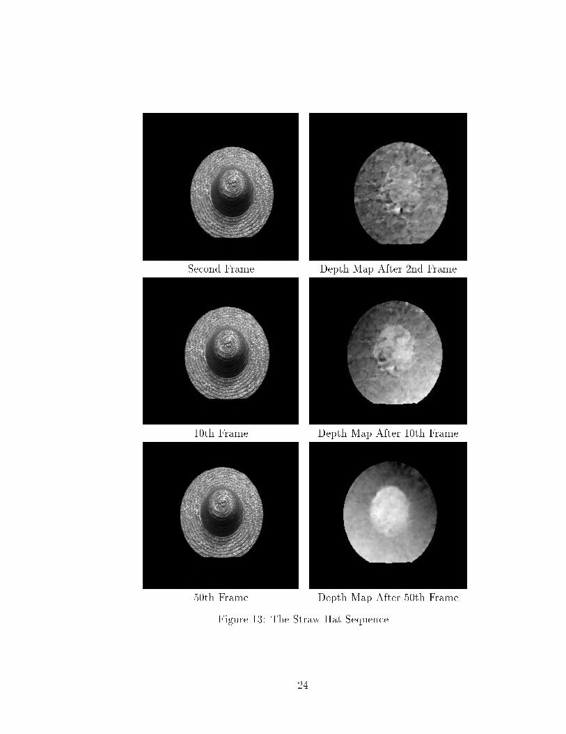
The �rst sequence includes �fty-one-frame images of a straw hat as we showed inthe previous section The images were digitized by a matrox board. The rotationsand translations of the camera with respect to the straw hat were discontinuous.The camera had about an 11� �eld of view. The optical ow and its uncertaintywere computed using hyper-geometric �lters [21, 22]. Figure 13 shows the intensityimages and depth maps computed after the corresponding frames. It clearly showsthe converging shape resulting from recursively combining information from multipleframes.

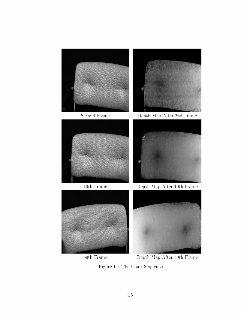
The Chair Sequence: The camera had an 22� �eld of view. The object was a realchair we used in our lab. The chair was rotating in front of the static camera as inFigure 14. Digitization was done by matrox board. The optical ow computationsometimes returned wrong results at some locations, which we believe were causedby texture aliasing. We can see that even in the tenth frame, the two buttons arevery clear in the depth map. Also noticeable is that part of the chair in the left sideis moving out and part of the chair in the right side is moving in. The move-in partis at �rst pretty noisy, and then gradually becomes smoother and smoother.

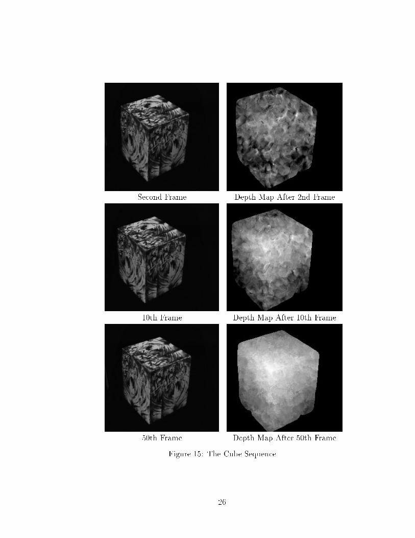
The Cube Sequence: The camera had about a 22� �eld of view. The sequence inFigure 15 was taken by a hand-held video camera connected to a Umatic recorder.It was recorded on a Umatic SP videotape and then digitized by a BVU digitizer,which could only capture one �eld in a frame. The digitized images have signi�cantlyhigher noise levels than those digitized by matrox board. We can see that the systemstill performs pretty well on those noisy images.

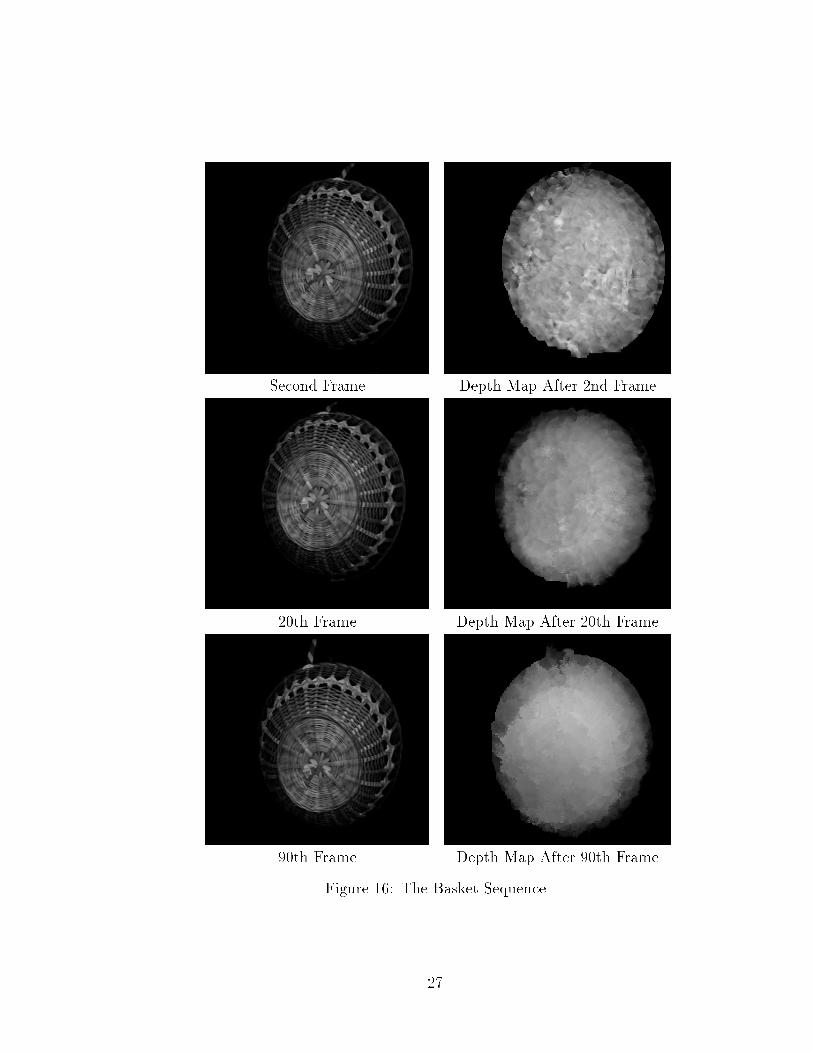
The Basket Sequence: The camera had a 22� �eld of view. The target was a basketwhich moving and rotating in front of the camera. The digitization was done the sameway as the cube sequence.

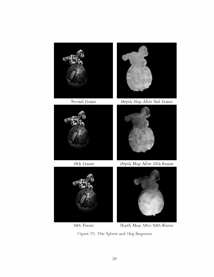
The Sphere and Dog Sequence: The camera had an 11� �eld of view. The targetwas a toy dog on top of a ball. The di�culties of this sequence are that (1) the ballhad a very low contrast near its boundaries; (2) it had obvious specular re ectionswhich will confuse the optical ow algorithm, and (3) the toy dog had a sparse texture.Despite these di�culties, our system still performs reasonably well as in Figure 17.The shape of the sphere and dog are both visible, and even the depth of the tail tipof the dog is correctly shown.

In all the experiments, the initial structure information was set as a at surfaceparallel to the image plane at depth 200 with independent uncertainty � = 100 atevery pixel. Despite such a crude initial estimation, there was no trouble caused bynonlinearity in our experiments.

From all these experiments, we conclude that our system of recursively recovering

23

Second Frame Depth Map After 2nd Frame

10th Frame Depth Map After 10th Frame

50th Frame Depth Map After 50th Frame

Figure 13: The Straw Hat Sequence

24

Second Frame Depth Map After 2nd Frame

10th Frame Depth Map After 10th Frame

50th Frame Depth Map After 50th Frame

Figure 14: The Chair Sequence

25

Second Frame Depth Map After 2nd Frame

10th Frame Depth Map After 10th Frame

50th Frame Depth Map After 50th Frame

Figure 15: The Cube Sequence

26

Second Frame Depth Map After 2nd Frame

20th Frame Depth Map After 20th Frame

90th Frame Depth Map After 90th Frame

Figure 16: The Basket Sequence

27

Second Frame Depth Map After 2nd Frame

10th Frame Depth Map After 10th Frame

50th Frame Depth Map After 50th Frame

Figure 17: The Sphere and Dog Sequence

28

dense structure from a dense optical ow sequence can converge to the true 3D shapeof the scene quickly and accurately. We have demonstrated its performance underadverse conditions such as noisy images, specularity, and texture aliasing. Even underthese conditions, the system performed robustly.

7 Summary

In summary, we presented an EKF-based system which recursively combine densestructural information from a sequence of optical ows. At current stage, our systemis able to deliver an evolving sequence of depth maps using optical ows. We alsoshowed that the system was very robust when the optical ows were noisy or containoutliers caused by texture aliasing and specularity.

Current representation of 3D dense information by depth maps and their uncer-tainty is very limiting in that complicated objects can not be represented. In thefuture, we would like to expand our system to deliver a �nal 3D model of the scenebased on the image sequence. In other words, we would like to maintain an indepen-dent module to store, retrieve and update 3D structural information. Therefore wecould extract a priori depth information from the module for every optical ow frame,and merge posteriori depth information into the module. The problem of representing3D dense structure and its uncertainty (independent and correlated) still remains tobe very challenging.

Acknowledgement

Thanks to Keith Gremban for pointing us to Sherman-Morrison-Woodbury formula.This research is sponsored by the Department of Army, Army Research O�ce undergrant number DAAH04-94-G-0006. The views and conclusions contained in this docu-ment are those of the authors and should not be interpreted as necessarily representingo�cial policies or endorsements, either expressed or implied, of the Department ofthe Army or the United States Government.

29

A Sherman-Morrison-Woodbury Inversion

Given a full-rank n�n matrix C, and its perturbed by a rank m matrix UVT , whereU and V are both n � m matrices, the Sherman-Morrison-Woodbury formula [9](page 225) states that

(C+UVT )�1 = C�1 �C�1U(Im +VTC�1U)�1VTC�1; (53)

where Im is the m�m unit matrix. The validity of this inverse can be easily veri�edby multiplying both sides by (C+UVT ).

In a more concise format, we can write the above equation as

(C+UVT )�1 = C1 +U1VT1 ; (54)

where

C1 = C�1; (55)

U1 = �C�1U(Im +VTC�1U)�1; (56)

V1 = C�TV: (57)

In our application, because C is a diagonal matrix, we can compute its inverse C1

accurately. Therefore the only source of numerical error is A = (Im +VTC�1U)�1.Suppose the error is

E = Im � (Im +VTC�1U)A; (58)

the �nal error is

(C+UVT )(C1 +U1VT1 )� I = UEVTC�1: (59)

Eq. 59 shows that there is a potential danger that the error E could be magni�edin the �nal error. That is the source of fragility of Sherman-Morrison-Woodburyformula. In our system, we reduce that risk by computing A is in double precisionand limiting the magni�cation factor (roughly the ratio between eigenvalues of UVT

and those of C) to be less than 104 as we did in Section 6.

30

B Eigen Analysis of Symmetric Outer Products

In this section, we consider eigen analysis and singular value decomposition of aspecial kind of matrices, i.e. symmetric outer products of two low-rank matrices.Because those matrices are symmetric, the problem of computing eigenvalues andeigenvectors is identical to the problem of singular value decomposition because

UVT =

0BBBBBB@~e1 ~e2 � � � ~em

1CCCCCCA

0BBBB@�1

�2. . .

�m

1CCCCA

0BBBB@

~eT1~eT2

...~eTm

1CCCCA ; (60)

whereU and V are both n�m (n >> m) matrices, �i; i = 1; 2; � � � ;m are eigenvalues,and ~ei; i = 1; 2; � � � ;m are normalized eigenvectors.

Theorem B.1 Suppose �0i ; i = 1; 2; � � � ;m and ~e0i ; i = 1; 2; � � � ;m are eigenvalues

and normalized eigenvectors of the m�m matrix VTU, we have the eigenvalues and

eigenvectors of n� n matrix UVT as

�i = �0i ; (61)

~ei =U~e0i

k U~e0i k; (62)

where k U~e0i k is the norm.

The proof of the above theorem is straightforward. Since �0i and ~e0i are an eigen-

value and eigenvector of VTU, we have

VTU~e0i = �0i~e0

i : (63)

Multiplying both sides by U, we obtain

(UVT )U~e0i = �0iU~e0

i : (64)

Thus we have the eigenvalue and eigenvector of UVT as �0i and U~e0i .

Additionally, if the outer product UVT is also positive semi-de�nite, which is trueif it represents covariance, we can rewrite it as

UVT = BBT ; (65)

where

B =

0BBBBBB@~e1 ~e2 � � � ~em

1CCCCCCA

0BBBB@

p�1 p

�2. . . p

�m

1CCCCA : (66)

31

References

[1] Golad Adiv. Determining three-dimensional motion and structure from optical ow generated by several moving objects. IEEE Transactions on Pattern Analysis

and Machine Intelligence, 7(4):384{401, July 1985.

[2] Golad Adiv. Inherent ambiguities in recovering 3-D motion and structure froma noisy ow �eld. IEEE Transactions on Pattern Analysis and Machine Intelli-

gence, 11(5):477{489, May 1989.

[3] A. Azarbayejani and Alex Pentland. Recursive estimation of motion, structure,and focal length. IEEE Transactions on Pattern Analysis and Machine Intelli-

gence, 1995. to appear.

[4] Edward J. Baranoski. Triangular factorization of inverse data covariance matri-ces. In International Conference on Acoustics, Speech, and Signal Processing,pages 2245{2248, Toronto, Canada, May 1991.

[5] Ted J. Broida, S. Chandrashekhar, and Rama Chellappa. Recursive estimationof 3D motion from a monocular image sequence. IEEE Transactions on Aerosp.

Electron. Syst., 26(4):639{656, July 1990.

[6] Anna R. Bruss and Berthold K. P. Horn. Passive navigation. Computer Vision,Graphics and Image Processing, 21:3{20, 1983.

[7] John J. Craig. Introduction to Robotics: Mechanics and Control. Addison-WesleyPublishing Company, Inc., second edition, 1989.

[8] Arthur Gelb, editor. Applied Optimal Estimation. The MIT Press, 1989.

[9] Gene Golub and James M. Ortega. Scienti�c Computing: An Introduction with

Parallel Computing. Academic Press, Boston, 1993.

[10] William W. Hager. Updating the inverse of a matrix. SIAM Review, 31(2):221{239, June 1989.

[11] David J. Heeger and Allan D. Jepson. Subspace methods for recovering rigidmotion I: Algorithm and implementation. International Journal of Computer

Vision, 7(2):95{117, 1992.

[12] Joachim Heel. Dynamic systems and motion vision. Technical Report AI Memo1037, MIT Arti�cial Intelligence Laboratory, 1988.

[13] Joachim Heel. Temporally integrated surface reconstruction. In Proceedings of

International Conference on Computer Vision, pages 292{295, 1990.

[14] H. C. Longuet-Higgins and K. Prazdny. The interpretation of a moving retinalimage. Proc. R. Soc. Lond. B, 208:385{397, 1980.

32

[15] Larry Matthies, Richard Szeliski, and Takeo Kanade. Kalman �lter-based al-gorithms for estimating depth from image sequences. International Journal of

Computer Vision, 3:209{236, 1989.

[16] William H. Press, Brian P. Flannery, Saul A. Teukolsky, and William T. Vetter-ling. Numerical Recipes in C. Cambridge University Press, 1988.

[17] J. Inigo Thomas and J. Oliensis. Incorporating motion error in multi-frame struc-ture frommotion. Technical Report COINS TR91-36, Computer and InformationScience, University of Massachusetts at Amherst, 1991.

[18] Carlo Tomasi. Shape and motion from image streams: A factorization method.Technical Report CMU-CS-91-172, The School of Computer Science, CarnegieMellon University, 1991.

[19] Roger Y. Tsai and Thomas S. Huang. Uniqueness and estimation of three-dimensional motion parameters of rigid objects with curved surfaces. IEEE

Transactions on Pattern Analysis and Machine Intelligence, 6(1), January 1984.

[20] Juyang Weng, Narendra Ahuja, and Thomas Huang. Closed-form solution +maximum likelihood: A robust approach to motion and structure estimation. InProceedings of Computer Vision and Pattern Recognition, pages 381{386, 1988.

[21] Yalin Xiong and Steven A. Shafer. Moment and hypergeometric �lters for highprecision computation of focus, stereo, and optical ow. Technical Report CMU-RI-TR-94-28, The Robotics Institute, Carnegie Mellon University, 1994.

[22] Yalin Xiong and Steven A. Shafer. Hypergeometric �lters for optical ow anda�ne matching. In International Conference on Computer Vision, 1995.

33