ENM 503 Block 2Lesson 8 Linear Models

The purpose of modeling is insight!

- famous old saying

Keep the roads

straight.

Narrator: Charles Ebeling 1

Today’s Models

Tracking inventory over time Linear programming The Leslie model

What a great choice of

examples of linear systems to

present to the class.

2

Tracking inventory over time

Let xi = inventory level at the end of month i (start of month i+1)

x0 = initial on-hand inventory

di = forecasted demands in month i

si = supply (due-in from supply or production) month i r = loss rate (damage, pilferage, deterioration, etc.)

applied to inventory at the start of the month onlyThen:xi = xi-1 – rxi-1 + si – di ; i = 0,1, 2, …

solve recursively!3

Tracking inventory

The N. Ven Tory Company maintains stock in its central warehouse on a popular appliance. They have 36 units currently in stock and have experienced no significant losses of these items. Other relevant data are:

xi+1 = xi-1 – rxi-1 + si – di

xjan = 36 + 10 -24 = 22 xFeb = 22 + 12 – 30 = 2xMar = 2 +12 – 18 = -4

Month demand due-in

Jan 24 10

Feb 30 12

Mar 18 12

4

Linear Programming

A Decision without optimization is like a arch

without a keystone or how to optimally allocate scarce

resources.

I have been wanting to optimally allocate scare resources for some time.

5

Our Very First Example

The Opti Mize Company manufactures two products that competefor the same (limited) resources. Relevant information is:

Product A B Available resources

Labor-hrs/unit 1 2 20 hrs/dayMachine hrs/unit 2 2 30 hrs/dayCost/unit $6 $20 $180/day

Profit/unit $5 $15

6

The ModelLet X = number of units of product A to manufacture Y = number of units of product B to manufacture

Max Profit = z = 5 X + 15 Y

subject to: X + 2 Y 20 (labor-hours)

2 X + 2 Y 30 (machine hours) 6 X + 20Y 180 ($ - budget)

X 0, Y 0

7

The Graphical Solution-1

X

Y

5 10 15 2520 30

5

10

20

15

X + 2 Y = 20

8

The Graphical Solution-2

X

Y

5 10 15 2520 30

5

10

20

15

X + 2 Y = 20

2X + 2Y = 30

9

The Graphical Solution-3

X

Y

5 10 15 2520 30

5

10

20

15

X + 2 Y = 20

2X + 2Y = 30

9

6X + 20Y = 180

The feasible region

10

The Graphical Solution-4(continued)

X

Y

5 10 15 2520 30

10

20

15

9 Z = 5X + 15Y = 30

2

6

4

Z = 5X + 15Y = 60

12

11

The Graphical Solution-5(continued)

X

Y

5 10 15 2520 30

10

20

15

9 Z = 5X + 15Y = 30

2

6

4

Z = 5X + 15Y = 60

12

(5, 7.5)

Z = 5 (5) + 15 (7.5) = 137.5

12

The Graphical Solution-6 Alternate Approach

X

Y

5 10 15 2520 30

5

10

20

15

9

Z = 5X + 15Y

(x = 15, y = 0; z = 75)(x = 0, y = 9; z = 135)

(x = 0, y = 0; z = 0)

13

The Graphical Solution-7 Alternate Approach

X

Y

5 10 15 2520 30

5

10

20

15

9(x = 10, y = 5; z = 125)

Z = 5X + 15Y

(x = 15, y = 0; z = 75)(x = 0, y = 9; z = 135)

(x = 0, y = 0; z = 0)

14

The Graphical Solution-8 Alternate Approach

X

Y

5 10 15 2520 30

5

10

20

15

9

(x = 5, y = 7.5; z = 137.5)

(x = 10, y = 5; z = 125)

Z = 5X + 15Y

(x = 15, y = 0; z = 75)(x = 0, y = 9; z = 135)

(x = 0, y = 0; z = 0)

15

This is powerful stuff!Can we see another example followed by adescription of the general model?

16

The Classical Diet Problem

Mr. U. R. Fatte has been placed on a diet by his Doctor (Dr. Ima Quack) consisting of two foods: beer and pizza. The doctor warned him to insure proper consumption of nutrients to sustain life. Relevant information is:

Nutrients Beer Pizza Weekly Requirement

I (Vit A) 2 mg/oz 3 mg/oz 3500 mgII 6 mg/oz 2 mg/oz 7000 mgIII 1 mg/oz 1 mg/oz 1000 mgcost/oz 10 cents 4.5 cents

17

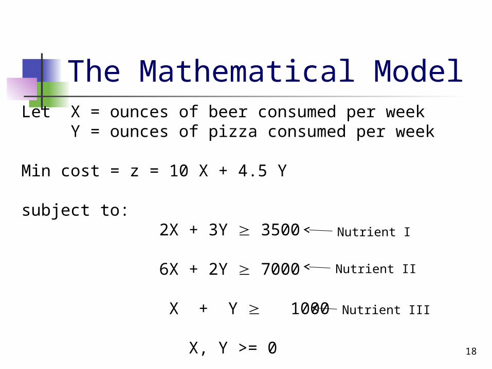
The Mathematical ModelLet X = ounces of beer consumed per week

Y = ounces of pizza consumed per week

Min cost = z = 10 X + 4.5 Y

subject to: 2X + 3Y 3500

6X + 2Y 7000

X + Y 1000

X, Y >= 0

Nutrient I

Nutrient II

Nutrient III

18

Graphical Solution to the Diet Problem-1

X

Y

1000

3000

2000

30002000

1000

40006x + 2y = 7000

2x + 3y = 3500

x + y =1000

Feasible Region

19

Graphical Solution to the Diet Problem-2

X

Y

1000

3000

2000

30002000

1000

40006x + 2y = 7000

2x + 3y = 3500

Z = 10x + 4.5y = 18000 cents

x + y =100020

Graphical Solution to the Diet Problem-3

X

Y

1000

3000

2000

30002000

1000

40006x + 2y = 7000

2x + 3y = 3500

Z = 10x + 4.5y = 18000 cents

(x = 1000, y = 500; z = 122.50)

x + y =100021

The General LP ModelMax or Min z = c1 x1 + c2x2 + . . . + cnxn

subject to: a11x1 + a12x2 + . . . + a1nxn b1

a21 x1 + a22x2 + . . . + a2nxn b2

.

. am1x1 + am2x2 + . . . + amnxn bm

x1, x2, . . . xn 0

Objective Function

Constraints

xj = decision variables or activity levelscj = profit or cost coefficientaij = technology coefficientbi = resource capacities (right hand side values)

22

The General LP Model in Matrix Form

11 12 1 1 1

21 22 2 2 2

1 2

...

..., ,

: : : : : :

...

n

n

m n n m

a a a x b

a a a x b

a a a x b

A x b

1 2 ... nc c c c

Max/Min

st :

z

cx

Ax b

x 023

Assumptions

Deterministic all input data (parameters) are known and constant no statistical uncertainty

Linear cost or profit is additive and proportional to the

activity levels output or resources consumed are additive and

proportional to the activity levels Non-integer

variables (activity levels) are real numbers

24

Solution Procedures Graphical

two or three variables only Algebraic

solve systems of equations for corner points Simplex algorithm

numerical, iterative approach Ellipsoid

theoretical importance more than applied

25

Can we seemore examplesof this LP thing?Please!!!!!

26

The Doit Wright Company – A Solver Solution

The Doit Wright Company manufactures three types of recreational vehicles within its five shops. Relevant data is provided in the following table.

Manufacturing times (hrs)

Shop Capacity (hrs/wk) Standard Fancy Luxury

Engine 120 3 2 1

Body 80 1 2 3

Standard finishing 96 2

Fancy finishing 102 3

Luxury finishing 40 2

Unit profit $840 $1120 $1200 27

FormulationS = number of standard’s made per weekF = number of Fancy’s made per weekL = number of Luxury’s made per weekMax profit = 840S + 1120F + 1200Lsubject to:

3S + 2F + L 120 S + 2F + 3L 802S 96

3F 103 2L 40

S, F, L 0

to a solver solution…

28

Engine

Body

Standard finishing

Fancy finishing

Luxury finishing

Solver Solution – check out the tutorial

Max profit = 840S + 1120F + 1200Lsubject to:

3S + 2F + L 120 S + 2F + 3L 802S 96

3F 103 2L 40

S, F, L 0

S F L840 1120 1200 profit

variables 20 30 0 50400 Obj Fcnconstraints sumprod RHS

3 2 1 120 120 1 2 3 80 80

2 40 963 90 103

2 0 40

29

The Leslie Model

Observe the population explosion!

30

About the Leslie Model

The Leslie Matrix is a discrete and age-structured model of population growth

It was invented by and named after P. H. Leslie. Describes the growth of populations (and their projected

age distribution) a population is closed to migration normally only one sex, usually the female, is considered

The population is divided into groups based either on age classes or life stage.

At each time step the population is represented by a vector where each element indicates the number of individuals currently in that class.

31

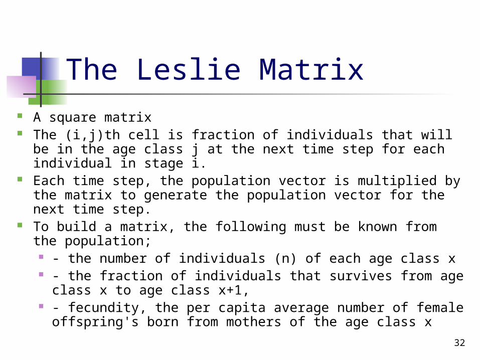
The Leslie Matrix A square matrix The (i,j)th cell is fraction of individuals that will be in the age

class j at the next time step for each individual in stage i. Each time step, the population vector is multiplied by the

matrix to generate the population vector for the next time step.

To build a matrix, the following must be known from the population;

- the number of individuals (n) of each age class x - the fraction of individuals that survives from age class x

to age class x+1, - fecundity, the per capita average number of female

offspring's born from mothers of the age class x32

The Math behind the Leslie Model

Let Δ = width of the age interval n = number of age groups n Δ = total number of yearsFi(t) = the number of females at time t in the ith age group

0

1

1

( )

( )

:

( )n

F t

F t

F t

F(t) t = 0, Δ, 2Δ, 3Δ, …

F(0) = current age distribution 33

More Math

di = death rate for the ith age group

pi = (1 – di) = fraction surviving

Fi+1(t + Δ) = pi Fi(t)

mi = maternity rate for the ith group

1

00

( ) ( )n

i it

F t m F t

newborns

Where is the matrix? I don’t see a matrix!

34

Now the Matrix

0 1 2 10 0

01 1

1

21 1

1

...( ) ( )

0 0 ... 0( ) ( )

0 0 ... 0: :

: 0 ... 0( ) ( )

0 0 ... 0

n

n nn

m m m mF t F t

pF t F t

p

pF t F t

p

, 0,1,2,

0k

t

k

F(t +Δ) MF(t)

F( Δ) M F( )

35

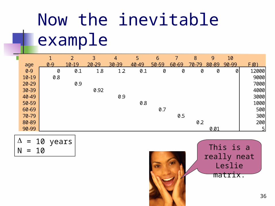
Now the inevitable example

= 10 yearsN = 10

1 2 3 4 5 6 7 8 9 10age 0-9 10-19 20-29 30-39 40-49 50-59 60-69 70-79 80-89 90-99 F(0)0-9 0 0.1 1.8 1.2 0.1 0 0 0 0 0 12000

10-19 0.8 900020-29 0.9 700030-39 0.92 400040-49 0.9 300050-59 0.8 100060-69 0.7 50070-79 0.5 30080-89 0.2 20090-99 0.01 5

This is a really neat

Leslie matrix.

36

The next 150 years…

1 2 3 4 5 6 7 8 9 10age 0-9 10-19 20-29 30-39 40-49 50-59 60-69 70-79 80-89 90-99 Total

F(0) 12,000 9,000 7,000 4,000 3,000 1,000 500 300 200 5 37,005F(1) 18,600 9,600 8,100 6,440 3,600 2,400 700 250 50 2 49,742F(2) 23,628 14,880 8,640 7,452 5,796 2,880 1,680 350 70 1 65,377F(3) 26,562 18,902 13,392 7,949 6,707 4,637 2,016 840 168 1 81,174F(4) 36,205 21,250 17,012 12,321 7,154 5,365 3,246 1,008 202 2 103,764F(5) 48,247 28,964 19,125 15,651 11,089 5,723 3,756 1,623 325 2 134,504F(6) 57,211 38,598 26,068 17,595 14,086 8,871 4,006 1,878 376 3 168,691F(7) 73,304 45,769 34,738 23,982 15,835 11,269 6,210 2,003 401 4 213,514F(8) 97,467 58,643 41,192 31,959 21,584 12,668 7,888 3,105 621 4 275,131F(9) 120,519 77,974 52,779 37,897 28,763 17,267 8,868 3,944 789 6 348,805F(10) 151,151 96,415 70,176 48,556 34,107 23,010 12,087 4,434 887 8 440,832F(11) 197,637 120,921 86,774 64,562 43,701 27,286 16,107 6,044 1,209 9 564,249F(12) 250,129 158,110 108,829 79,832 58,106 34,961 19,100 8,054 1,611 12 718,743F(13) 313,312 200,103 142,299 100,123 71,848 46,485 24,472 9,550 1,910 16 910,118F(14) 403,480 250,649 180,093 130,915 90,110 57,479 32,539 12,236 2,447 19 1,159,969F(15) 515,342 322,784 225,584 165,686 117,824 72,088 40,235 16,270 3,254 24 1,479,091

37

The Journey Ends

We have walked the straight (linear) and narrow path.

Next we will walk that same path however more

discretely.38