University of Calgary

PRISM: University of Calgary's Digital Repository

Graduate Studies The Vault: Electronic Theses and Dissertations

2017

Enhancing Hydrocarbon Recovery and Sensitivity

Studies in Tight Liquid-Rich Gas Resources

Wang, Min

Wang, M. (2017). Enhancing Hydrocarbon Recovery and Sensitivity Studies in Tight Liquid-Rich

Gas Resources (Unpublished master's thesis). University of Calgary, Calgary, AB.

doi:10.11575/PRISM/25905

http://hdl.handle.net/11023/3850

master thesis

University of Calgary graduate students retain copyright ownership and moral rights for their

thesis. You may use this material in any way that is permitted by the Copyright Act or through

licensing that has been assigned to the document. For uses that are not allowable under

copyright legislation or licensing, you are required to seek permission.

Downloaded from PRISM: https://prism.ucalgary.ca

UNIVERSITY OF CALGARY

Enhancing Hydrocarbon Recovery and Sensitivity Studies in Tight Liquid-Rich Gas Resources

by

Min Wang

A THESIS

SUBMITTED TO THE FACULTY OF GRADUATE STUDIES

IN PARTIAL FULFILMENT OF THE REQUIREMENTS FOR THE

DEGREE OF MASTER OF SCIENCE

GRADUATE PROGRAM IN CHEMICAL AND PETROLEUM ENGINEERING

CALGARY, ALBERTA

MAY, 2017

© Min Wang 2017

ii

Abstract

Unconventional tight reservoirs refer to the formations with a permeability ranges from 0.001 to

0.1 millidarcy. Horizontal drilling coupled with multistage hydraulic fracturing is required in these

formations to achieve economic production rates. Recovery factor in tight gas formations is

typically less than 25% of the original gas in-place. Such low recovery is a strong motivation to

investigate the application of enhancing hydrocarbon recovery methods in these reservoirs.

In this study, enhanced hydrocarbon recovery methods are investigated for a Montney liquid rich

gas reservoir, located in the Western Canadian Sedimentary Basin. Firstly, a heterogeneous

reservoir model is built and history-matched based on the production data collected from the field.

Production performance of three EHR methods including cycling gas injection, CO2 flooding and

water injection are then compared and their economic feasibility are evaluated. Sensitivity analysis

of operational and geological factors including primary production duration, bottom hole pressures

(BHP) during primary production and EHR process, pressure-dependent matrix permeability, non-

Darcy effects and hydraulic fracture conductivity is conducted and their effects on the well

production performance are studied. Experimental design is adopted to further study the

mechanism and optimize the enhancing recovery process by cyclic gas injection and CO2 injection.

Results show that both cumulative oil and gas production are increased with fluid injection

compared to primary depletion methods. In addition, cyclic gas and CO2 flooding is more feasible

for the ultra-low unconventional tight gas reservoir than water flooding due to the water injection

difficulty and low sweep efficiency in the reservoir. Cycling gas injection leads to both a higher

gas and oil recovery and lower injection cost due to the on-site available gas source and minimal

transport/purchase costs, gaining more economic benefits than that of CO2 flooding. Thus, it can

iii

be concluded that cyclic gas flooding in tight liquid rich gas reservoirs with hydraulically

stimulated fractures could be a good way to enhance oil and gas production. Optimization study

results indicate that two injection wells, short primary production time, high primary BHP and

injection BHP, short injection time and low later period BHP lead to an optimal scheme of cyclic

gas flooding and CO2 flooding methods.

iv

Acknowledgements

I would like to thank my nice supervisor Dr. Shengnan (Nancy) Chen, who keeps providing

guidance, support and encouragement during my master study at the University of Calgary.

I would also like to thank my respectable examination members: Dr. Zhangxing Chen and Dr. Brij

Maini for their encouragement, valuable suggestions and insightful comments.

I would like to deliver the gratitude to my colleagues and friends for their help during my master

study. I also appreciate the help from Reservoir Simulation Group and the support from the Seven

Generations Energy Ltd.

Last but not the least, I would like to express my appreciation to my family for their love, support

and encouragement.

ii

Table of Contents

Abstract ................................................................................................................................2 Acknowledgements ..............................................................................................................4

Table of Contents ................................................................................................................ ii List of Tables ..................................................................................................................... iv List of Figures and Illustrations ...........................................................................................v List of Symbols, Abbreviations and Nomenclature .......................................................... vii

CHAPTER ONE: INTRODUCTION ..................................................................................1

1.1 Overview ....................................................................................................................1 1.2 Problem Statement .....................................................................................................2 1.3 Objectives ..................................................................................................................4

1.4 Outline .......................................................................................................................5

CHAPTER TWO: LITERATURE REVIEW ......................................................................7 2.1 Unconventional Tight Reservoir ................................................................................7

2.2 Tight Oil .....................................................................................................................8 2.3 Tight Gas ....................................................................................................................9

2.4 Hydraulic Fracturing in Tight Reservoirs ................................................................16 2.5 Enhanced Recovery Method in Tight Reservoir ......................................................19 2.6 Gas Injection Method ...............................................................................................21

2.6.1 Lean Gas Injection Method .............................................................................22 2.6.2 Nitrogen Injection Method ..............................................................................24

2.6.3 CO2 Injection Method ......................................................................................26 2.6.4 Huff-n-puff Method .........................................................................................27

2.7 Water Injection Method ...........................................................................................29

CHAPTER THREE: ENHANCING HYDROCARBON RECOVERY IN TIGHT LIQUID-

RICH GAS RESOURCES ........................................................................................31 3.1 Geologic Model .......................................................................................................32 3.2 Reservoir Simulation Model ....................................................................................37

3.2.1 Model Description ...........................................................................................37 3.2.2 Hydraulic Fracture – Local Grid Refinement ..................................................41 3.2.3 PVT Model ......................................................................................................42 3.2.4 History Match ..................................................................................................44

3.3 Enhanced Hydrocarbon Recovery methods .............................................................45 3.3.1 Reservoir Performance ....................................................................................45 3.3.2 Phase Envelop Change ....................................................................................51

3.3.3 NPV Calculation ..............................................................................................53 3.4 Conclusions ..............................................................................................................54

CHAPTER FOUR: SENSITIVITY STUDIES ON CYCLIC GAS FLOODING

PERFORMANCE .....................................................................................................56

4.1 Effect of BHP ...........................................................................................................56 4.2 Effect of Different Primary Production Time ..........................................................59 4.3 Pressure-dependent Permeability .............................................................................63

iii

4.4 The Effect of Non-Darcy Flow in Hydraulic Fractures ...........................................66

4.5 Hydraulic Fracture Height .......................................................................................67 4.6 Hydraulic Fracture Conductivity .............................................................................69 4.7 Conclusion ...............................................................................................................72

CHAPTER FIVE: OPTIMIZATION OF GAS INJECTION IN TIGHT LIQUID RICH GAS

RESERVOIR ............................................................................................................74 5.1 Parameters Considered in the Simulation Model ....................................................74

5.1.1 Number of Injection Wells ..............................................................................76 5.1.2 Parameters of Primary Production ...................................................................77

5.1.3 Parameters of Injection ....................................................................................78 5.2 Experimental Design ................................................................................................78 5.3 Results and Discussion ............................................................................................87

5.4 Conclusion ...............................................................................................................94

CHAPTER SIX: CONCLUSIONS AND FUTURE WORK ............................................96 6.1 Conclusions ..............................................................................................................96

6.2 Future work ..............................................................................................................98

REFERENCES ..................................................................................................................99

iv

List of Tables

Table 2-1 Marketable natural gas production in Canada (NEB, 2014) ........................................ 10

Table 2-2 Ultimate potential for Montney unconventional petroleum in British Columbia and

Alberta ................................................................................................................................... 14

Table 3-1 Reservoir model properties........................................................................................... 39

Table 3-2 Gas and liquid components table .................................................................................. 43

Table 3-3 Cumulative production for different enhanced hydrocarbon methods ......................... 51

Table 3-4 NPV for different enhanced hydrocarbon methods ...................................................... 54

Table 4-1 Data of the Cumulative production under different well BHPs ................................... 59

Table 4-2 Production data of different primary production time .................................................. 63

Table 4-3 Pressure-dependent permeability table (Cho, 2013) .................................................... 65

Table 5-1 Simulation parameters combinations of cyclic gas flooding ........................................ 82

Table 5-2 Simulation parameters combinations of CO2 flooding ................................................. 85

Table 5-3 Calculated Revenue of cyclic gas flooding .................................................................. 91

Table 5-4 Calculated Revenue of CO2 flooding ........................................................................... 93

v

List of Figures and Illustrations

Figure 2-1 Geological view of the WCSB (Canadian Society of Western Exploration

Geophysicists) ......................................................................................................................... 8

Figure 2-2 Canadian tight oil production (NEB, 2015) .................................................................. 9

Figure 2-3 Tight and shale gas production from 2000 to 2013 (NEB, 2015) ............................... 11

Figure 2-4 Natural gas processing plant ....................................................................................... 12

Figure 2-5 Location of the Montney Formation in the subsurface of Alberta and British

Columbia. (Modified from the Geological Atlas of the Western Canada Sedimentary

Basin.) ................................................................................................................................... 13

Figure 2-6 Mixed hydrocarbon distribution (Momentum Oil & Gas LLC, 2011) ....................... 15

Figure 2-7 Schematic of hydraulic fractured wells (NEB, 2015) ................................................. 17

Figure 2-8 Two dimensional models (Gidley et al. 1989) ............................................................ 18

Figure 2-9 P-T diagram of a retrograde condensate (Larry, 2007) ............................................... 19

Figure 2-10 Huff-n-puff schematic (NETL) ................................................................................. 29

Figure 3-1 Kakwa area type log (Kuppe et al. 2012) .................................................................... 33

Figure 3-2 Four horizons and wells location ................................................................................ 34

Figure 3-3 Mixed hydrocarbon system (Kuppe et al., 2012 ) ....................................................... 34

Figure 3-4 3D View of geologic model ........................................................................................ 36

Figure 3-5 Properties of the geological model .............................................................................. 36

Figure 3-6 Accumap view of well pads ........................................................................................ 38

Figure 3-7 3D view of simulation model containing target wells ................................................ 39

Figure 3-8 Permeability and porosity variation of the simulation model ..................................... 40

Figure 3-9 Relative permeability curves for Montney formation ................................................. 41

Figure 3-10 Local refined grids near the hydraulic fracture ......................................................... 42

Figure 3-11 P-T diagram ............................................................................................................... 44

Figure 3-12 History matching result for well-3 ............................................................................ 45

vi

Figure 3-13 Cumulative oil and gas production of various injection fluids ................................. 48

Figure 3-14 The Impact of injection fluids on reservoir pressure during production time........... 50

Figure 3-15 P-T diagram of different gas oil ratios during cyclic gas injection ........................... 52

Figure 3-16 P-T diagram of different gas oil ratios during CO2 injection .................................... 52

Figure 4-1 Cumulative production under different well BHPs ..................................................... 58

Figure 4-2 Comparison of different primary production time ...................................................... 62

Figure 4-3 Average field pressure ................................................................................................. 62

Figure 4-4 Comparison of two cases with and without pressure compactions ............................. 65

Figure 4-5 Comparison of Darcy and non-Darcy flow ................................................................. 67

Figure 4-6 Cumulative oil production under two fracture heights ............................................... 69

Figure 4-7 Cumulative production of the two cases ..................................................................... 71

Figure 5-1 2D View of the Simulation Model .............................................................................. 75

Figure 5-2 3D View of simulation models ................................................................................... 77

Figure 5-3 Graphical example of Lk full factorial experimental designs ...................................... 80

Figure 5-4 CO2 fraction in the late injection period ..................................................................... 84

Figure 5-5 Gas saturation in the 2D simulation model of cyclic gas flooding ............................. 89

Figure 5-6 Pressure distribution in the 2D simulation model of cyclic gas flooding ................... 90

Figure 5-7 Revenue value distribution of the 32 tests of cyclic gas flooding ............................... 91

Figure 5-8 Revenue value distribution of the 32 tests of CO2 flooding ........................................ 93

vii

List of Symbols, Abbreviations and Nomenclature

Symbol Definition

𝐶𝑤𝑒𝑙𝑙 Cost of horizontal well

𝐶𝑓𝑟𝑎𝑐𝑡𝑢𝑟𝑒 Cost of hydraulic fracture

𝐶 Total cost

i Interest rate

n Number of periods

𝐹𝐶 Total fixed cost

N Number of horizontal wells

𝑉𝑔𝑎𝑠 Value of gas revenue

𝑉𝑜𝑖𝑙 Value of oil revenue

𝑉𝐹 Future value of gas and condensation liquid revenue

μ Viscosity

v Velocity

k Hydraulic fracture permeability

β Non-Darcy Beta factor

ρ Density of certain phase

𝐶𝑓𝑑 Dimensionless hydraulic fracture conductivity

𝑘𝑓 Fracture permeability

𝑤𝑓 Fracture width

𝑘𝑚 Matrix permeability

𝐿𝑓 Hydraulic feature half-length

𝑘𝑒𝑓𝑓 Effective permeability

𝑤𝑔𝑟𝑖𝑑 Grid width

1

Chapter One: Introduction

1.1 Overview

Canada, the fifth largest natural gas producer of the world, occupies 5% of the gross global gas

production. The country’s natural gas production is mainly supplied by the Western Canadian

Sedimentary Basin (WCSB), which contains substantial natural gas and oil reserves, such as oil

sands, heavy oils, conventional resources, and unconventional tight/shale resources. The

productivity of unconventional gas formations has grown rapidly due to further exploration and

development, while the production of conventional natural gas has decreased.

Except for small numbers of dry gas producers, heavy hydrocarbon components (e.g., ethane,

propane, butanes and pentanes plus) will separate from the gas state in the form of liquids when

raw natural gas comes from the wellhead. This wet gas, liquid rich gas or natural gas liquid (NGL),

composes an important part of Canada’s energy mix.

The deep part of the Western Canada Sedimentary Basin indicates significant potential for

unconventional gas resources. In this basin, the Montney Formation is considered one of Canada’s

most potential economic gas plays (NEB, 2010). The formation covers approximately 130,000

square kilometres and spans 700 kilometres north to south, traversing the provincial boundary

between northwest Alberta and northeast British Columbia (Seven Generation, 2017).

2

The average daily production in the Montney formation is around 3.5 billion cubic feet of natural

gas per day (Bcf/d), accounting for 25% of natural gas production in the WCSB. Even though the

area’s development is still in the preliminary stages, its estimated potential is noteworthy. The

formation contains 449 trillion cubic feet (tcf) of marketable gas, 14,521 million barrels of

marketable natural gas and 1,125 million barrels of marketable oil.

Hydraulic fracturing in horizontal wells is the main method for extracting products from liquid

rich tight reservoirs. The process is established and commercially successful. During hydraulic

fracturing, tons of fracturing fluid and proppants are pumped into the reservoir matrix to create

hydraulic fractures, significantly improving gas recovery.

1.2 Problem Statement

Pressure depletion is the main recovery method used for the primary production period of tight

liquid rich gas reservoirs. Liquid will drop out when the reservoir pressure decreases below the

dew point, resulting in condensate liquid accumulating in the formation and around the wellbore.

The accumulation blocks the gas flow path, decreasing the gas condensate production significantly

(Moses and Donohoe, 1965; Hichman and Barree, 1985; Vo et al. 1989; Pope et al., 2000; Li and

Abbas, 2000).

Low permeability and low porosity are characteristics of tight and shale reservoirs. The condensate

liquid blocking problem is exacerbated significantly by the ultra-low reservoir permeability and

3

gas production rate could be reduced by 50%-80% in a gas condensate sandstone reservoir within

the first two years (Ayyalasomayajula et al., 2005).

To solve this problem, lean gas injection (Smith and Yarborough, 1968; Abel et al., 1970; Sigmond

and Cameron, 1977; Abasov et al., 2000), CO2 injection (Chaback and Williams, 1994; Goricnik

et al., 1995) and N2 injection (Aziz, 1982) were investigated by several researchers. Their studies,

however, focused on the conventional reservoirs only.

The pressure depletion method by horizontal wells with multistage hydraulic fractures is the

current application for exploring gas condensate in tight reservoirs formations. IOR or EOR

methods have not been largely applied in shale and tight gas condensate reservoirs. Yu et al. (2014)

employed a numerical simulation method to study the efficiency of CO2 injection to enhance gas

recovery in the shale reservoir, considering the adsorption of CO2 in the shale with a high total

organic content. A sensitivity analysis of the CO2 injection lead to the optimal assessment of the

best scenario through the experimental design method. Sheng (2015) constructed a simulation

model of a gas condensate tight reservoir to study the efficiency of enhancing gas and oil recovery

by gas injection, CO2 injection and water flooding. The results indicate that the huff-n-puff gas

injection is a more practical and effective method to enhance gas and oil recovery than CO2 and

water injection. The study, however, used a simplified simulation model containing a single

fracture instead of a multistage fractured horizontal well. More literatures can be found in the

literature review chapter.

4

1.3 Objectives

This study focuses on enhancing hydrocarbon recovery by gas injection in the tight liquid rich gas

condensate reservoir, conducting a sensitivity study of the key parameters and optimizing a gas

injection scheme and controlling crucial factors. A geological model which contains 27 horizontal

wells are built through Petrel and three wells are cut out to build a simulation model, each well

containing about 30 stages of hydraulic fractures, in a tight liquid rich gas reservoir. The interactive

contact of nearby wells and pressure distribution/interaction are considered. The aim is to develop

a simulation study to enhance liquid rich gas and oil recovery at the late stage of the pressure

depletion process in a tight condensate reservoir and to determine a best scenario to maximize gas

and oil recovery.

The detailed objectives are:

(1) To build a comprehensive reservoir model based on field data collected from public domain

and validate such model by the production data.

(2) To investigate the performances of three scenarios of enhanced hydrocarbon recovery methods,

including cycling gas injection, CO2 injection and water injection and compare their economic

feasibility for the target reservoir.

5

(3) To conduct a sensitivity study on the key parameters, including fracture conductivity, stress

compaction, non-Darcy effect, primary production time and production BHP to investigate their

effects on the enhancing hydrocarbon process in the target tight gas reservoir.

(4) To perform an experimental design (DOE) to create a series of reservoir simulations combined

with variable parameters to maximize the NPV from the target reservoir.

1.4 Outline

A summary of the content of Chapters Two to Six follows:

(1) Chapter Two delivers a detailed literature review related to the topic of this thesis, including a

detailed forecast of unconventional tight reservoirs, hydraulic fractures and the EOR or IOR

methods of gas injection, CO2 injection and water injection.

(2) Chapter Three focuses on the construction of the heterogeneous simulation model and the use

of three EHR methods after primary production period to prevent reservoir pressure decline,

complement formation energy and enhance gas and oil recovery.

(3) Chapter Four investigates the sensitivity study of the operational and geological factors,

including primary production duration, bottom hole pressures (BHP) during primary production

and EHR process, matrix permeability and non-Darcy effects.

6

(4) Chapter Five employs an experimental design to calculate a series of combinations of

simulations to that optimize the gas injection method in tight liquid rich gas reservoir. This work

overrides the time-consuming shortcomings of the traditional “vary one parameter at a time”

strategy, significantly saving time and energy.

(5) Chapter Six lists the conclusions and future recommendations resulting from this study.

7

Chapter Two: Literature Review

2.1 Unconventional Tight Reservoir

The Western Canadian Sedimentary Basin (WCSB), situated in Western Canadian, spans the

southwest corner of the Northwest Territories, the northeast of British Columbia and Alberta

southern Saskatchewan and southwestern Manitoba, as shown in Figure 2-1. The basin contains

substantial natural gas and oil reserves, such as oil sands, conventional resources, and

unconventional resources. Different from conventional resources, unconventional resources,

including coalbed methane, tight gas, tight oil and shale gas, are stored in formation with low

porosity and permeability, leading to low recovery efficiency without special stimulation

treatments (e.g., horizontal drilling technique and hydraulic fracturing).

This thesis focuses on the study of tight reservoir, featured with low porosity and permeability,

small drainage radius and low productivity, which is composed with sandstone, siltstone, limestone

and carbonates. The development of tight reservoir requires significant well stimulation mainly

including hydraulic fracturing technique, horizontal wells treatment and multi-lateral wells to

improve the recovery to meet the economic value.

8

Figure 2-1 Geological view of the WCSB (Canadian Society of Western Exploration

Geophysicists)

2.2 Tight Oil

Tight oil is a kind of light crude oil contained in low permeability reservoirs which needing

horizontal drilling and multi-stage hydraulic fracturing technique. Tight oil in the WCSB started

to be developed in the Bakken Formation of southeast Saskatchewan and southwest Manitoba in

2005 and latterly had spread extensively to Alberta with the main formations like Cardium. In

2014, the production of tight oil accounted for over 10 percent of total Canadian crude oil

production. Figure 2-2 shows the growth trend of tight oil production in the past several years. The

production grew from near zero in 2005 to 350,000 barrels per day in 2013.

9

Figure 2-2 Canadian tight oil production (NEB, 2015)

2.3 Tight Gas

Natural gas production in Canada is mainly supplied by the WCSB in British Columbia, Alberta,

and Saskatchewan, and other smaller regions in offshore Nova Scotia, Ontario, New Brunswick,

and Nunavut. Table 2-1 shows the constituent parts of Canada’s total gas production in 2014.

Canada is the fifth largest natural gas producer of the world, occupying 5% of the gross global gas

production. With the further exploration and development of unconventional resources, the

productivity of unconventional natural gas has grown rapidly while the production of conventional

natural gas has decreased.

10

Table 2-1 Marketable natural gas production in Canada (NEB, 2014)

In 2014, tight and shale gas accounted for about 51 percent of total Canadian natural gas

production. Figure 2-3 shows Canadian shale and tight gas production from 2000 to 2013. Gas

production grew from three billion cubic feet per day in 2000 to seven billion cubic feet per day

by 2013. By 2035, tight and shale gas production together is expected to occupy 80 percent of

Canada’s natural gas production (NEB, 2015).

Marketable Production (MMcf/d)

Province NS NB ON SK AB BC YT Canada

Total

Mar. 354 10 7 427 9,781 3,897 13 14,488

Apr. 364 10 7 446 10,017 4,014 11 14,869

May 346 9 11 446 9,732 3,952 12 14,506

Jun. 436 10 11 423 9,469 3,689 11 14,049

Jul. 390 8 10 441 9,899 3,846 11 14,606

Aug. 281 9 12 436 9,994 4,022 11 14,765

Sep. 174 9 12 443 9,630 3,946 10 14,224

Oct. 161 9 12 443 10,249 4,163 9 15,046

Nov. 224 8 12 433 10,183 4,201 10 15,070

Dec. 301 9 12 432 10,423 4,320 12 15,509

11

Figure 2-3 Tight and shale gas production from 2000 to 2013 (NEB, 2015)

Dry gas is mostly composed of methane. According to the U.S. Energy Information Administration

(EIA), dry gas is defined as what remained after all the heavier hydrocarbons (hexane, octane, etc.)

and non-hydrocarbons (helium, nitrogen, etc.) are removed from the natural stream. Wet gas

contains heavier hydrocarbons such as ethane and butane and less than 85% methane. During the

production process, heavy hydrocarbon components (e.g., ethane, propane, butanes and pentanes

plus) will separate from the gas state in the form of liquids when raw natural gas comes from the

wellhead. If the liquid yield greater than 10 bbls from every MMcf sales gas when flowing through

a gas processing plant, the gas is considered “liquid-rich”.

12

This wet gas is called liquid rich gas or natural gas liquids (NGL), composing an important part of

Canada’s energy mix. Most NGLs are produced at the natural gas processing plants (Figure 2-4),

located primarily in the gas- producing areas of Alberta and several plants in British Columbia.

The Deep Basin part of the WCSB indicates that natural gas accounts for significant resource

potential in Canada’s energy mix.

Figure 2-4 Natural gas processing plant

This thesis focuses on producing low-cost, liquids-rich natural gas from the Montney geological

formation, an elongated oval-shaped, lower-Triassic sedimentary basin composed of sandstones,

siltstones and carbonates, which covers approximately 130,000 square kilometres and spans 700

kilometres north to south, traversing the provincial boundary between northwest Alberta and

northeast British Columbia (Seven Generation, 2017). The depth of the formation is very thin on

its eastern and northeastern sides, while very thick, usually ranging from 100 m to 300 m at its

13

western edge. Due to the increase of depth causing increasing pressure and decreasing natural gas

liquids (NGL) and oil content, the reservoir characteristics vary extensively over the formation.

Figure 2-5 Location of the Montney Formation in the subsurface of Alberta and British

Columbia. (NEB, 2013)

The Montney, containing one of the biggest marketable unconventional gas resources, is

considered one of Canada’s most potential economic gas plays. In 2012, its average daily

production rose to an average of 48.6 million m3/d (1.7 Bcf/d), while the total Canadian marketable

gas production was about 392.7 million m3/d (13.9 Bcf/d) (NEB, 2013). Even though Montney

14

development is still in the early stages, its forecast for increased gas production places it in a key

role in Canada’s overall production.

The ultimate potential for unconventional petroleum in the Montney total production is composed

of both the British Columbia and Alberta portions. As shown in Table 2-2 the ultimate expected

marketable volume of natural gas is 12,719 billion m³, while marketable NGLs is 2,308 million

m³ and marketable oil is 179 million m³ (1,125 million barrels).

Table 2-2 Ultimate potential for Montney unconventional petroleum in British Columbia

and Alberta (NEB, 2013)

Hydrocarbon

Type

In-Place

Low

In-Place

Expected

In-Place

High

Marketable

Low

Marketable

Expected

Marketable

High

Natural Gas

(billion m³)

90,559 121,080 153,103 8,952 12,719 18,257

NGLs

(million m³)

13,884 20,173 28,096 1,540 2,308 3,344

Oil

(million m³)

12,865 22,484 36,113 72 179 386

The content of NGLs out of natural gas varies widely from a liquid rich gas (50 bbl/MMcf

condensate) to a light crude system (3,350 scf/bbl), from west to east, with a coinciding rise of

every vertical depth of 100 m.

15

The unconventional Montney reservoir is characteristic of overpressure with a gradient range from

10.5 kPa/m to 13.5 kPa/m; the gradient difference exceeds 3 kPa/m, stretching over 20 kilometers.

The dynamic behind the large pressure difference is stems from the slow migration of gas, over

millions of years, from the original hydrocarbon generation, pushing oil to the upper structure with

lower pressure and accumulating into the upper trapped reservoirs. The hydrocarbon composition

of the Montney area is quite variable even within small areas, as discerned by numerous analyses

of gas/liquid ratios and liquid yields. The liquid and gas failed to be re-dispersed more uniformly

due to the low and less diverse combined matrix and natural fracture permeability. Thus, a mixed

hydrocarbon schematic forms (Frank el at., 2012). The transition of dry gas to oil is rough and

uneven; the wet gas areas in the transition region vary largely (Figure 2-6).

Figure 2-6 Mixed hydrocarbon distribution (Momentum Oil & Gas LLC, 2011)

16

2.4 Hydraulic Fracturing in Tight Reservoirs

Low reservoir permeability and porosity in tight formations impede the flow of oil and gas into

the wellbore without the application of stimulation methods. Hydraulic fracturing is the process of

pumping fluid into the wellbore at an injection rate which is high enough to force the formation to

crack. During the process of fluid injection, the resistance towards the flow increases

accumulatively, leading to the increase of pressure to reach an ultimate value called break-down

pressure, composed of the in-situ compressive stress and the strength of the formation. A hydraulic

fracture is created when fracturing liquid is pumped into the pay zone at a high enough rate to

reach the break-down pressure.

At the beginning, a neat fluid, called a ‘pad’, is pumped to initiate the fracture and to establish

propagation. Fluid, mixed with a propping agent (proppant), is injected. This ensures that, in the

event of the pumping operation ceasing, the fractures are kept separated; the pressure in the fracture

decreases below the compressive in-situ stress trying to close the fracture. The fracture is extended

continuously and then the proppant is carried by the slurry into the deeper part of the fracture. At

the late stage, when the injected fluid begins to flow back with a lower viscosity to the wellbore,

a propped fracture with much higher conductivity is created, allowing oil and gas to flow,

unimpeded, from the tight formation into the wellbore.

Hydraulic fracture propagation is influenced significantly by a series of factors, such as the

variation of in-situ rock stresses, variations of pore pressure, bonding of formations, relative bed

thickness of formations near the fractures, mechanical rock properties, and fluid pressure gradients.

17

Typically, horizontal fractures are easily generated at shallow depths while vertical fractures tend

to be created in deeper areas. The higher lateral stress above and below the target formation

constrains the growth of vertical fractures. Fracture height influences the halt length and fracture

configuration significantly. Figure 2-7 shows two forms of hydraulic fractures along horizontal

and vertical wells. With successful applications of multi-stage hydraulic fracturing treatments in

horizontal wells in tight formations, production has increased significantly in recent years.

Figure 2-7 Schematic of hydraulic fractured wells (NEB, 2015)

The hydraulic fracture properties, such as length, width and height, cannot be measured during the

field treatment. The only measurable parameters are the volume of the injected fracturing fluid and

the time to complete the process. Various models are created to predict fracture properties,

including two dimensional models, pseudo three dimensional models, and fully three dimensional

18

models. The most common two dimensional models are the Perkins-Kern-Nordgren (PKN) and

Kristonovich-Geertsma-de Klerk (KGD). The PKN model is used when the fracture length is much

greater than the fracture length. The KGD model is applied when the fracture height is more than

the fracture length, as shown in Figure 2-8.

(a) PKN geometry for a 2D fracture (b) KGD geometry for a 2D fracture

Figure 2-8 Two dimensional models (Gidley et al. 1989)

Tight reservoirs, however, are more complex. Horizontal wells are applied in tight reservoirs due

to their low permeability and porosity. Multiple staged hydraulic fractures are closely spaced along

the horizontal wellbores and the hydraulic fracture of the adjacent wells also tends to transmit

communication pressure. Consequently, in tight reservoirs, the hydraulic fractures are influenced

by many other stress changes from nearby fractures and the adjacent wells. The oversimplified

fracture model fails to describe the hydraulic fractures in tight reservoirs (Olson et at., 2012). In

Olson’s study, a non-planar fracture model simulates complex hydraulic fracture propagation.

19

2.5 Enhanced Recovery Method in Tight Reservoir

Under some special reservoir condition, gas will condensate as liquid when the reservoir pressure

drops below the dew point pressure, as shown in Figure 2-9. The reservoir pressure is point A, at

the initial gas state. When the pressure drops from A to B, liquid appears in the gas phase, opposite

to the regular discipline that the liquid phase will be vaporized as a gas phase when pressure

decreases. The phenomenon is known as retrograde condensate; reservoirs displaying this

condition are considered as retrograde condensate reservoirs.

Figure 2-9 P-T diagram of a retrograde condensate (Larry, 2007)

The development and operation of gas condensate reservoirs differ greatly from crude-oil and dry-

gas reservoirs. A wholly vapor phase always exists at the time of exploration with an initial

pressure above the dew point pressure and a temperature above the critical temperature. Pressure

depletion is the main recovery method during the previous production period. Liquid will drop out

20

when the reservoir pressure decreases below the dew point, resulting in condensate liquid

accumulation around the wellbore. The condensate liquid collects near the wellbore, largely

blocking the gas flow rate and decreasing the gas condensate well production significantly (Moses

P L and Donohoe, 1965; Hichman and Barree, 1985; Vo et al. (1989); Pope et al., 2000; Kewen

Li, and Abbas, 2000).

Tight and shale reservoirs are characteristic of low permeability and low porosity. The pressure

gradient is generally large during the pressure depletion process, which means the rate of growth

and expansion of the condensate bank around the wellbore will be relatively high. Consequently,

the condensate liquid blocking problem is exacerbated significantly by low reservoir permeability

and high production rate (Wheaton and Zhang, 2000). The condensate liquid blocking could reduce

the well recovery by 50%-80% in a gas condensate sandstone reservoir (Ayyalasomayajula et al.,

2005). The productivity factor could be reduced by a factor of 10 in the low permeability reservoir

with 0.15 md (Lin and Finley, 1985). As a result, many studies have been conducted to deal with

the problem of low recovery in gas condensate reservoirs, especially in low permeability reservoirs

(e.g., tight reservoirs and shale reservoirs). The main enhanced condensate recovery methods

explored include natural gas injection, CO2 injection, nitrogen injection and water injection.

As compared with conventional reservoirs, gas injection in tight and shale liquid rich reservoirs

has recently attracted attention. Gas and water injection are seen as the main stimulation methods.

Gas injection includes gas flooding and huff-n-puff modes. In tight and shale reservoirs,

permeability and porosity are extremely low and the pressure gradient is larger during the depletion

process. The condensate blocking problem, therefore, becomes more prominent. The current

technique to produce oil and gas in tight reservoirs is through multiple transverse fractured

21

horizontal wells relying on primary pressure depletion. The study of unconventional plays shows

that, although the reservoir characteristics vary greatly, in the primary production period,

production declines rapidly, leading to a low recovery factor, ranging from 3% to 5% of the total

original oil in place (Liu et al. 2014). The oil recovery factor in oil-saturated shale reservoirs is

very low; for instance, in the Bakken formation, the recovery is approximately 7% (Clark et al.,

2009). At the late production period, massive shale oil remains unproduced unless stimulated

methods are employed. In Lake’s study (Lake et al., 2014), enhanced oil recovery processes are

classified into the following methods: solvent, polymer, surfactant, foam-enhanced oil recovery

and thermal. Research has been conducted to explore ways to address gas condensate issues during

depletion production.

2.6 Gas Injection Method

The gas condensate reservoir is initially saturated with natural gas, with an initial pressure above

the dew point pressure. Once the reservoir pressure drops below the dew point pressure, liquids

will come out from the gas state. Compared with gas, oil is more difficult to flow to the surface.

Condensate oil collecting around the wellbore, blocking the gas flow significantly, adds to the

challenge (Hernandez et al., 1999; Thomas et al., 1995).

Juell and Whitson (Juell et al., 2013) found an optimal production strategy. In the initial stage, the

bottom hole pressure is equal to the saturation pressure, and eventually decreases. In the long term,

however, when the pressure drops below the dew point pressure, the liquid oil will condensate

during the gas phase and accumulate at the wellbore, blocking the gas flowing rate. Thus,

22

maintaining pressure higher than the dew point pressure is essential to prevent liquid condensate

from forming in the later period. The most widely used pressure maintenance method is

revaporization by lean gas flooding (Standing et al., 1948; Weinaug and Cordell, 1949; Smith and

Yarborough, 1968; Abel et al., 1970; Abasov et al., 2000). Nitrogen and CO2 flooding are also

used effectively.

2.6.1 Lean Gas Injection Method

Early in 1948, researchers began to investigate revaporization of liquid condensate. Standing et al.

(1948) performed laboratory tests of the revaporization of liquid condensate using the gas cap in

variable permeability systems and computed the butanes and heavier fraction condensate after

pressure decline. The results revealed that if the reservoir pressure drops down to the upper dew

point pressure followed by lean gas cycling, a lower cycling pressure contributes better to the

butanes’ recovery. Since then, further research has focused on the factors affecting the optimum

methods for exploring a gas condensate reservoir.

Weinaug and Cordell (1949) investigated the influence of revaporization through the use of two

systems of methane-n-butane and methane-n-pentane and one type of sand pack. Their results

indicated that with the presence of sand, the condensate liquids can be revaporized by a sufficient

injection gas.

Oxford & Huntington (1952) studied the influence of various factors including, the rate of gas

flow, original liquid saturation reservoir temperature. They also explored how desorption of

23

hydrocarbons from unconsolidated sand was affected by the presence of water and brine in both

pressure depletion and constant pressure flow methods.

Smith and Yarborough (1968) investigated revaporization in the retrograde condensate recovery

through dry gas injection into a long sand pack. Three rounds of methane revaporization from an

n-pentane-methane mixture with the presence of immobile water were performed in their two

water-wet experiments and one oil-wet test. The fourth-round experiment was conducted by a

methane-hydrogen sulfide mixture revaporized without the presence of water saturation. The

results show that all the heavier components could be recovered by sufficient dry gas injection.

Abel et al. (1970) investigated a two-dimensional, three-phase compositional model to analyze the

effect of revaporization of liquids in a retrograde condensate reservoir in the Carson Creek field,

cycled below the dew point pressure. Three schemes of gas injection included: normal cycling

with low rate gas sales, partial cycling with normal rate gas sales, and reservoir depletion without

gas injection. The results indicate that partial cycling scheme is optimal, resulting in higher

recovery of liquids with better economical assessment in the long run.

Sigmond and Cameron (1977) conducted experiments to investigate the influence of particle size,

initial liquid saturation, dry gas injection rate and immobile water saturation on the revaporization

process in gas condensate reservoirs. The reinjection of cyclic gas for the purpose of improving

formation pressure made it generally uneconomic.

24

More recently, Abasov et al. (2000) detailed the compositional behavior of a lean gas condensate

when depleted in a PVT cell at 1000 C (data for different temperatures are not given). The physical

properties of condensates were collected in the condenser at different pressure intervals during the

four isothermal depletion processes. Special attention was paid to the evaporation of the remaining

liquid condensate after depletion upon contact by lean natural gas. They concluded that more

elevated temperatures result in higher evaporation effectiveness, or recovery, of condensate by

lean gas.

2.6.2 Nitrogen Injection Method

The increasing value of sales gas reduces the commercial assessment to divert the gas from the

sale line (Aziz et al., 1982, Buchanan et al., 1981). Thus, researchers focused on nitrogen, with its

advantages of low price and stable properties, as a substitute for natural gas to maintain pressure

during the cycling operation.

Wilson and Moses (1981) conducted experiments to evaluate the ability of maintaining reservoir

pressure and displacement efficiency of nitrogen in a retrograde gas-condensate reservoir. The

reservoir fluid was studied through static equilibrium tests in a windowed equilibrium cell. The

injected natural gas or nitrogen was mixed with reservoir fluid and the mixture improved the dew

point. The test indicates that retrograde liquid loss will happen in the displacing front in the mixing

region; nitrogen gas injection shows greater mixture effectivity. To further study the mixture

influence on the phase behavior during the reservoir displacement operation, a packed-column

displacement apparatus was built using lean gas and nitrogen, respectively, as displaced injection

25

gases. Both injection methods showed over 98% recovery of fluid and infinite gas/liquid ratio in

the sand tube. The significant liquid recovery indicates that little mixing occurs during the lean

gas/ gas and nitrogen/ gas displacement during the packed-column displacement experiments.

Although the static equilibrium tests and packed-column experiments demonstrated different

liquid loss, nitrogen gas proved similar effectiveness with natural gas in displacing the retrograde

condensate fluid. The liquid flowing in porous media is dominated by the streamline effect of

Darcy's law. The extent of mixing is affected by reservoir heterogeneity, mobility ratio, flow

pattern, molecular diffusion and dispersion under the actual reservoir conditions. Thus, mixing

will be reduced by controlling the above factors. Compared with lean gas, the mobility ratio of

nitrogen injection is more stable and more easily maintained. If the injection and production rates

are controlled, flow pattern changes could be minimized.

Buchanan et al. (1981) investigated the economic feasibility of using nitrogen as an alternative to

natural gas during the cycling operation. Three nitrogen injection scenarios were created. Factors,

such as gas prices, stock-tank liquid content, and the degree of reservoir heterogeneity, were

considered. The study indicated that a gas reservoir containing liquid richer than 100 bbl/MMcf

should be considered for potential nitrogen injection.

In a study of Eckles et al. (1981) in the Fordoche Field, USA, injected natural gas was shown to

be more readily miscible with displaced liquids in the hot and high-pressured sands, when the

initial bottom hole pressure was about 11,018 psig and the bottom hole temperature was 278°F.

As the cost of natural gas increases rapidly, a mixture of natural gas and nitrogen is considered as

a more economic substitute. The mixture of 30% nitrogen and 70% natural gas was injected as

26

make-up gas after a previous injection of natural gas. The nitrogen is blocked against the reservoir

oil and gas by the previous injected natural gas. The previous injected gas can also be displaced

and recovered by the nitrogen mixture. In rich retrograde condensate-gas reservoirs, one problem

with nitrogen injection is that mixing it with condensate liquid will lead to significant in-situ

condensate drop-out. The experiment indicated that liquid drop-out takes place in the system, in

both the methane and nitrogen injection front. The methane creates less liquid drop-out than does

the nitrogen and shows better PVT static behaviour under the condition of mixing with the

condensate liquids.

If the Peclet number, a ratio of convective mass transfer to dispersive mass transfer, is high,

however, the dispersion scale is insignificant, which will cause less negative influence on recovery.

If the Peclet number is low, the nitrogen injection causes lower oil recovery than does the methane

injection. If the Peclet number is high enough, the nitrogen injection recovery approaches that of

the natural gas injection (Sigmund and Cameron, 1977). Gas injection will inevitably raise the dew

point pressure, leading to an incomplete recovery of liquid. Thus, recovery is partially influenced

by the pressure/composition (p-x) behavior of the injection gas and condensate fluid.

2.6.3 CO2 Injection Method

Chaback and Williams (1994) investigated the p-x behavior of a rich gas condensate reservoir with

CO2 and N2-CO2 mixture injections under two reservoir temperatures (2150 F and 316°F) and

high pressure. The PVT test indicated that the CO2 injection is more efficient than the N2-CO2

mixture in revaporizing retrograde liquid.

27

Goricnik et al. (1995) conducted experiments to compare the effect of CO2 and natural gas using

pressure-composition and pressure-retrograde liquid dropout diagrams. The results demonstrated

that CO2 achieved more efficiency than natural gas in revaporizing retrograde liquid in the gas

condensate reservoir.

A sensitivity analysis in a dry gas reservoir in Barnett reservoir was conducted by Yu et al, (2014)

to study CO2 injection in improving recovery. The result indicated that CO2 injection is an effective

way to enhance gas recovery.

2.6.4 Huff-n-puff Method

The huff-n-puff (Figure 2-10) injection scheme entails injecting a well with a recovery

enhancement fluid and, after a soaking period, returning the well to production. Huff-n-puff can

include either gas or CO2. In a gas condensate reservoir, pressure depletion is the main recovery

method. To improve production, large pressure differences and an optimal flowing are needed. In

the depletion mode, optimal operation conditions exist for liquid rich gas tight reservoirs.

Gamadi et al. (2013) are the first to launch studies on the performance of huff-n-puff gas injection

in shale oil reservoirs. A shale core plug, saturated with oil, was placed inside a large container

saturated with gas. The space between the core plug and container was regarded as fractures.

Initially, the gas pressure increased more than did the oil in the core plug; the gas was pushed into

the core plug, which imitates the injection period. After a gas soaking period, the pressure on the

28

gas declined below the core pressure. The oil in the core plug was displaced, which represents the

puff period. The analysis of the effects of the soaking pressure and soaking time on oil recovery

showed that soaking pressure had a more significant effect on oil recovery than did soaking time.

The study indicated that maintaining pressure in shale and tight reservoirs is the leading

mechanism to enhance oil and gas production.

Wan et Al, (2013) simulated the huff-n-puff method through a black oil model in a shale oil

reservoir. Their result shows that cycle time is a significant factor in incremental oil recovery. The

optimal huff-n-puff scheme is to use a shorter injection time and longer production time.

After the earlier study on the huff-n-puff method in shale oil reservoirs (Wan et al., 2013; Gamadi

et al., 2013, 2014; Wan et al., 2014), a series of simulations were conducted to investigate it in in

a shale gas condensate reservoir (Sheng, 2014; Sheng, 2015; Meng and Sheng 2015). In a

simplified simulation model containing one well with two half-length fractures as injector and

producer, huff-n-puff shows greater advantage than gas flooding in many aspects, such as early

response to gas injection, high drawdown pressure, effective evaporation to decrease oil saturation

near the wellbore, and averting pressure transport due to low reservoir permeability. They

concluded that the huff-n-puff method has the capacity to improve oil and gas recovery more

effectively than natural gas flooding and pressure depletion.

29

Figure 2-10 Huff-n-puff schematic (NETL)

According to Yu et al, (2014), the CO2 huff-n-puff method did not show significant efficiency

because, during the puff phase, a large amount of injected CO2 flows back to the surface in advance

of the natural gas. The separation of mixed CO2 and natural gas also increase costs.

2.7 Water Injection Method

Water flooding is another technique used to boost gas condensate reservoirs’ recovery (Hernandez

et al., 1999). Hernandez’s study investigated continuous and simultaneous gas cycling with water

injection (CSGW) and continuous gas cycling with alternating water injection (CGAW). They

concluded that water is not only a good reservoir void space filler, but also increases the mobility

ratio, improves the sweep efficiency and enhances recovery significantly.

30

Mattews et al. (1988) conducted experimental and theoretical studies focused on the feasibility of

water injection in gas condensate reservoirs. They concluded that water flooding was advantageous

in improving oil and gas recovery as compared with original pressure depletion methods.

Cullick et al. (1993) investigated simulation work on the water-alternating-gas process (WAG), in

which water and gas are combined in water flooding. A compositional reservoir simulation model

was set up to study the influence of different parameters. The results show that the WAG method

is more effective in improving condensate reservoir production than is pure gas injection.

In this study, cyclic gas flooding, CO2 flooding and water flooding are investigated in a

heterogeneous simulation model in a tight liquid rich gas condensate reservoir. The efficiency of

the three methods to enhance hydrocarbon recovery are compared. The optimization study is also

conducted to maximize the tight reservoir recovery.

31

Chapter Three: Enhancing Hydrocarbon Recovery in Tight Liquid-Rich Gas Resources

The development of the hydraulic fracturing technique in horizontal wells to produce natural gas

from tight liquid rich gas reservoirs has increased over the past few years in North America and is

playing a crucial role in the world’s energy supply. When field pressure drops below the reservoir

dew point pressure, however, oil will be condensate out of the gas phase during the pressure

depletion process. The oil remains unproduced in the reservoir, bringing profound changes from

single phase to two-phase flow, which can reduce well productivity. Thus, pressure maintenance

is critical in maximizing gas and oil recovery in the Montney Formation.

In this study, a simulation model for a liquid rich gas reservoir in Montney formation is established

and history-matched to optimize well performance and pressure maintenance through cycling gas

flooding, CO2 flooding and water flooding methods. More specifically, a heterogeneous geological

model containing 27 parallel horizontal wells is created based on the geologic data collected from

the Montney formation, while a section with 3 horizontal wells is cut out for the numerical

simulations. A PVT model is constructed based on sampling and experimental data, then the model

is validated by history match. Daily well bottom-hole pressure and gas-oil production data are used

to estimate and adjust the model parameters. After the primary production, three scenarios of EHR

methods, including cyclic gas flooding, CO2 flooding and water flooding, are employed to

maintain and increase oil and gas production. The EHR efficiency and economic estimation are

compared and optimized. The influence of injected cyclic gas on the PVT model is also

investigated.

32

3.1 Geologic Model

The Montney formation is a foremost example of unconventional gas plays in the Western

Canadian Sedimentary Basin, covering an area of 130,000 square kilometers from northeast British

Columbia to northwest Alberta. The formation consists of siltstone and dark grey shale, with fine

grained sandstone on the top and dolomitic siltstone in the base. It has unconformable contact

between the Doig formation (in the above layer) and the Belloy formation (in the lower layer).

The depth of the Montney ranges from 2800 m to 3500 m; the average formation thickness is 200

m. The two production zones - the upper Montney and the lower Montney - contain 449 trillion

cubic feet of marketable natural gas, 14,521 million barrels of marketable natural gas liquids and

1,125 million barrels of oil, as estimated by Canada’s National Energy Board. A middle Montney

wedge, which is not pervasive throughout the entire area, spreads between the upper and lower

Montney, separating the two main intervals, as shown in Figure 3-1. Multiple hydraulic fractures

placed along the horizontal wells is the main completion method in the Montney area to achieve

commercial production rates (Kuppe et al.2012).

The geological model (34,000 m × 18,000 m × 200 m), containing 27 horizontal wells in this study

is built by PETREL (Schlumberger), based on a block in a liquid-rich gas reservoir in the Great

Kakwa area of the Montney formation. Structural surfaces are built based on well tops where four

horizons - Doig, top Montney, middle Montney and low Montney are generated. The horizons

consist of three zones: the top Montney zone (Doig to top Montney), the middle Montney zone

(top Montney to middle Montney) and the low Montney zone (middle Montney to low Montney)

33

(Figure 3-1). Most of the horizontal wells underlie the upper Montney and overlie the low

Montney, spreading into the middle Montney zone. The same trend appears in the wells shown in

Figure 3-2 and Figure 3-3.

Figure 3-1 Kakwa area type log (Kuppe et al. 2012)

34

Figure 3-2 Four horizons and wells location

Figure 3-3 Mixed hydrocarbon system (Kuppe et al., 2012 )

35

The depth of the Montney top to the surface ranges from 2800 m to 3500 m and average formation

thickness is 200 m. The model consists of 4,896,000 grids, including 680 grids in the I direction,

360 grids in the J direction and 20 grids in the K direction. The geological model and collected

wells are shown in Figure 3-4.

The formation is characterized as being over-pressured, lacking aquifer and having variable

liquid/gas rations, which, combined, leads to the thermal cracking of the oil, forming gases over

geological time (Figure 3-3). Due to the higher temperature in the deeper part of the Montney,

thermal cracking is continuous and generates enormous gas, resulting in mixed hydrocarbons and

an over-pressured system. Thus, the gas is forced by the overly high pressure to migrate to the

upper dip, forming a regional pressure gradient (Kuppe et al.,2012).

Figure 3-5 depicts the permeability and porosity distribution of the geological model, where the

matrix permeability ranges from 0.004 to 0.009 md, porosity is between 2% and 9%, and connate

water saturation is 30%.

36

Figure 3-4 3D View of geologic model

(a) matrix permeability distribution (b) ) porosity distribution

Figure 3-5 Properties of the geological model

37

3.2 Reservoir Simulation Model

3.2.1 Model Description

The geological model is updated and imported into the CMG, creating an original simulation

model. The gas-liquids concentrations in Montney is determined by formation temperature,

pressure and facies. Pad 2, Pad 8 and Pad 19 (Figure 3-6) are the main research fields of this study.

Based on the geological model, the numerical simulation model is created. First, the geological

model constructed by Petrel is upscaled. Then, a target model, including three wells as shown in

Figure 3-7, is cut out as a sub-model and exported directly into CMG GEM to create the simulation

model.

The length of the multi-fractured well-1 is 2,500 meters with 28 stages, well-2 is 2,100 meters with

27 stages and well-3 is 3,000 meters with 31 stages. The average stage spacing is 80 m and the

perforation type is open-hole. The reservoir model has the dimensions of 1,050 m x 3,800 m x 60

m. There are 21 grids in the I direction, 76 grids in the J direction and 7 grids in the L direction,

which corresponds to the reservoir model’s width, length, width and thickness. Local refining grids

are generated to represent the hydraulic fractures in the reservoir model.

38

Figure 3-6 Accumap view of well pads

The properties of the heterogeneous simulation such as initial reservoir condition, permeability,

porosity and hydraulic properties, are listed in Table 3-1. Relative permeability curves of the

matrix are obtained from a reference paper (Lan, 2015) on experiments of sample studies from the

Montney tight gas play, as shown in Figure 3-9. In hydraulic fractures, the relative permeability

curves are applied as two straight lines.

39

Table 3-1 Reservoir model properties

Reservoir temperature (℃) 98

Reservoir Pressure (MPa) 30.5

Matrix permeability(md) 0.004~0.009

Matrix porosity 0.02~0.09

Matrix water saturation 0.3

Dew point pressure (MPa) 21.2

Hydraulic facture half-length (m) 125

Hydraulic facture height (m) 40

Primary facture width (m) 0.008

Intrinsic permeability (md) 8000

Figure 3-7 3D view of simulation model containing target wells

40

(a) Permeability distribution

(b) Porosity distribution

Figure 3-8 Permeability and porosity variation of the simulation model

41

(a) Oil and water relative permeability curve (b) Liquid and gas relative permeability curve

Figure 3-9 Relative permeability curves for Montney formation

3.2.2 Hydraulic Fracture – Local Grid Refinement

To make the hydraulic fracture model more explicit, local grid refinement is adopted to create

smaller and more accurate grids to simulate the hydraulic fracture. The local grid refinement of

the hydraulic fracture is shown in Figure 3-10.

42

Figure 3-10 Local refined grids near the hydraulic fracture

Assuming that the conductivity of the actual fracture is equal to the conductivity in the fracture

fairway blocks in the simulation model:

𝑘𝑒𝑓𝑓 ∙ 𝑤𝑔𝑟𝑖𝑑 = 𝑘𝑓 ∙ 𝑤𝑓

The minimum grid block width in the simulation cannot be smaller than the well radius. The

fracture grid is equals to the smallest grid width, which is set to 2 feet.

3.2.3 PVT Model

The area of interest is a liquid rich gas zone. Oil and gas samples are collected from the separator

and recombined with the production gas oil ratio of 1200m3/m3 to analyze the phase behavior of

the reservoir fluids. Table 3-2 shows the gas and liquid components. Accurate evaluations of gas-

oil ratios are crucial for the history matching and oil and gas production forecasts. Based on raw

data from sampling and laboratory PVT tests, the PVT models were developed and the reservoir

fluid system were estimated. Figure 3-11 depicts the calculated phase envelope of the recombined

fluid. The dew point temperature is 64℃ and the dew point pressure is 23.2 MPa. The reservoir

43

condition (98 ℃, 30.5 MPa) belongs to the retrograde condensation area of the generated phase

envelope, as shown in Figure 3-11.

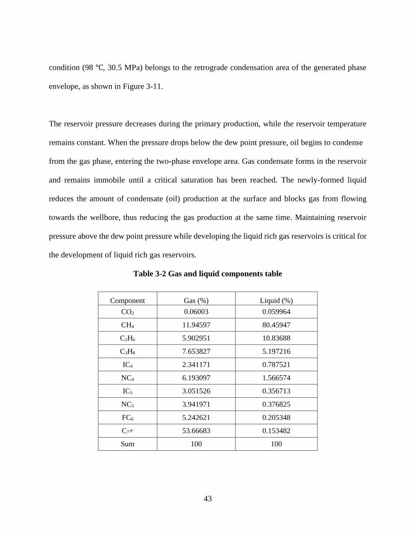
The reservoir pressure decreases during the primary production, while the reservoir temperature

remains constant. When the pressure drops below the dew point pressure, oil begins to condense

from the gas phase, entering the two-phase envelope area. Gas condensate forms in the reservoir

and remains immobile until a critical saturation has been reached. The newly-formed liquid

reduces the amount of condensate (oil) production at the surface and blocks gas from flowing

towards the wellbore, thus reducing the gas production at the same time. Maintaining reservoir

pressure above the dew point pressure while developing the liquid rich gas reservoirs is critical for

the development of liquid rich gas reservoirs.

Table 3-2 Gas and liquid components table

Component Gas (%) Liquid (%)

CO2 0.06003 0.059964

CH4 11.94597 80.45947

C2H6 5.902951 10.83688

C3H8 7.653827 5.197216

IC4 2.341171 0.787521

NC4 6.193097 1.566574

IC5 3.051526 0.356713

NC5 3.941971 0.376825

FC6 5.242621 0.205348

C7+ 53.66683 0.153482

Sum 100 100

44

Figure 3-11 P-T diagram

3.2.4 History Match

History matching was performed to tune the reservoir simulation model. The bottom-hole

pressures of the producers were applied as constraints while oil and gas rates were matched. Figure

3-12 shows the history matching result for well-3. It can be seen that, the gas rate and oil rate

match well with the production history. The production history has been honored and the model is

accurate and reliable enough for reservoir simulations and production predictions. The model can

also be used to evaluate the performance of enhanced recovery methods, which are reported in the

next section.

45

(a) Gas rate history match (b) Oil rate history match

Figure 3-12 History matching result for well-3

3.3 Enhanced Hydrocarbon Recovery methods

3.3.1 Reservoir Performance

As aforementioned, it is essential to keep the reservoir pressure above the dew point pressure for

a liquid rich gas reservoir, as indicated by the phase diagram. Primary production studies suggest

that the average reservoir pressure drops to 22.8 MPa after 6 years of depletion, as shown in the

base case in Figure 3-14. The base case represents the scenario where the primary production is

applied. The P-T diagram of the reservoir fluids (see Figure 3-11) has suggested that liquid would

be condensed out below such pressure and reservoir fluids enters the two-phase region. Pressure

maintenance technique needs to be applied by injecting fluids into the reservoir to keep a preferable

pressure in the formation. Thus, Well-2, which locates in the middle, is then converted into an

46

injection well while well-1 and well-3 are kept as producers. Water, CO2 and cyclic gas are injected

into the formation, respectively, for 10 years to increase reservoir pressure.

It should be noted that the cyclic gas flooding is different from the cyclic gas huff-n-puff method.

In the cyclic gas flooding, the separated gas produced from the production wells is injected into

the injection well continuously to maintain the reservoir pressure. While for the cyclic gas huff-n-

puff method, the produced gas from the puff period is separated and re-injected into the same well

during the huff period. The huff and puff operations are conducted via the same producer and no

particular injector is needed.

Figure 3-13 shows the cumulative gas and oil production of cyclic gas flooding, CO2 flooding, and

water flooding for the targeted formation. The injection pressure for all three scenarios are 45 MPa.

As aforementioned, the base case represents the scenario of primary production without any

injection. Cyclic gas flooding leads to the highest gas and oil cumulative production, as compared

with the CO2 and water injection cases. It should be noted that Figure 3-13a depicts the total

cumulative gas production, which contains produced CO2 for the CO2 flooding and a portion of

injected natural gas for the cyclic gas scenario. Take CO2 flooding for example, although the total

gas production rate is higher than that of the base case, the cumulative gas production of the CO2

injection scenario is lower than the base case after removing the CO2 from the produced mixture.

Table 3-2, which demonstrates that the cumulative natural gas production are close among

different scenarios while that of the base case is slight higher than the rests.

47

Cyclic gas flooding and CO2 flooding both enhance cumulative oil production significantly. The

cumulative oil production of the cyclic gas flooding is 52.7% higher than that of the base case and

CO2 flooding indicates a 40.0% improvement in cumulative oil production as shown in Figure 3-

13b. It indicates the applicability of cyclic gas flooding in the liquid rich gas reservoirs. In addition,

the water injection scenario results in a lower cumulative gas production but a higher cumulative

oil production than those of the base case scenario. This is because the injected water reduces the

relative permeability of the gas phase, decreasing its ability to flow to the wellbore. Meanwhile

the higher reservoir pressure due to water injection helped preventing oil from condensing in the

reservoir.

There is a high gas saturation near well-2 for the cyclic gas flooding and needs to be re-produced

at the end of the enhanced hydrocarbon recovery process. After 10 years’ injection, well-2 is

converted back into a producer and put on production. A large amount of gas and oil are produced

during such process, significantly increasing both the cumulative gas and oil production. It should

be noted that the volume of the injected gas needs to be subtracted to achieve the net cumulative

gas production for cyclic gas flooding. Table 3-2 shows the calculated net natural gas production

of the four scenarios.

48

(a) Cumulative gas production

(b) Cumulative oil production

Figure 3-13 Cumulative oil and gas production of various injection fluids

49

Figure 3-14 compares the reservoir pressure of the base case with that of the cyclic gas, CO2 and

water injection scenarios during the production period. The primary production period is from the

beginning to 2190 days. At that point, the production well-2 is converted into an injection well and

different injection scenarios are conducted.

The figure shows that the reservoir pressure increases for all the injection scenarios, while the

cyclic gas flooding scenario indicates the highest rise in reservoir pressure, followed by the CO2

and water scenarios. All injection scenarios share the same injection pressure of 45 MPa at the

injector. Well-2 of the cyclic gas flooding scenario, is opened to production again at 5475 days;

the average reservoir pressure starts to drop fast since this process starts. An intense pressure

drawdown exists between the reservoir formation and well bottom hole, which leads to a

significant enhancement of oil and gas production. Overall, cyclic gas flooding is the most

effective for improving the average pressure. CO2 flooding has the secondary ability to improve

reservoir pressure, while water flooding sits at third place, due to the low porosity and permeability

of shale reservoirs and weak liquid injection capacity.

50

Figure 3-14 The Impact of injection fluids on reservoir pressure during production time

The barrel of oil equivalent (BOE) is adopted to assess the gas and oil productivity. BOE is

industrial unit of energy equivalent to the amount of energy released by burning one barrel of crude

oil. The calculated BOE results are shown in Table 3-2. Cyclic gas flooding displays the largest

BOE calculation, followed by CO2 flooding, base case and water flooding. In addition, the BOE

of the water flooding is lower than that of the base case. This is because the injected water has

decreased the effective gas permeability in the formation, leading to a lower gas production rate.

In other words, the increase of oil production due to a higher reservoir pressure during water

flooding cannot compensate for the loss of gas production, as compared with the base case. The

51

cumulative oil production of the base case is the lowest among all scenarios, as the low reservoir

pressure of the base case promotes oil to be condensed and left unproduced in the reservoir.

Table 3-3 Cumulative production for different enhanced hydrocarbon methods

Cyclic gas CO2 Water Base case

Cumulative injected volume (m3) 1.00×109 1.71×109 1.51×106 0

Cumulative natural gas production (m3) 2.60×109 1.60×109 1.52×109 1.74×109

Net cumulative gas production (m3) 1.60×109 1.60×109 1.52×109 1.74×109

Cumulative oil production (m3) 576,924 528,924 421,922 377,781

BOE 1.43×107 1.39×107 1.25×107 1.34×107

NPV ($) 3.11×108 2.50×108 2.40×108 2.69×108

3.3.2 Phase Envelop Change

The phase diagram will change during the cyclic gas flooding and CO2 flooding process due to the

compositional change of the reservoir fluids. Figure 3-15 and Figure 3-16 show the new phase

diagram with the production GOR equaling 1500 and with CO2 injection. It can be seen that both

the critical pressure and temperature decrease and the two-phase region shifts to the left, compared

52

to Figure 3-11. Such changes will help prevent the oil condensation in the formation under

reservoir condition and further increase the oil production at the surface.

(a) Original P-T diagram without gas injection (b) P-T diagram with cyclic gas injection

Figure 3-15 P-T diagram of different gas oil ratios during cyclic gas injection

(a) Original P-T diagram without gas injection (b) P-T diagram with CO2 injection

Figure 3-16 P-T diagram of different gas oil ratios during CO2 injection

53

3.3.3 NPV Calculation

The net present value of the enhanced hydrocarbon recovery processes has been briefly estimated

via the following equation (Yu and Sepehrnoori, 2014):

𝑁𝑃𝑉 = ∑(𝑉𝑜𝑖𝑙+𝑉𝑔𝑎𝑠−𝐶𝐹)𝑗

(1+𝑖)𝑗 − [∑ (𝐶𝑤𝑒𝑙𝑙 + 𝐶𝑓𝑟𝑎𝑐𝑡𝑢𝑟𝑒) + 𝐹𝐶𝑁𝑘=1 ]𝑛

𝑗=1 (3-1)

Where 𝑉𝑜𝑖𝑙 and 𝑉𝑔𝑎𝑠 are annual gas and oil revenue, 𝐶𝐹 is all the related cost due to injection,

𝐶𝑤𝑒𝑙𝑙 and 𝐶𝑓𝑟𝑎𝑐𝑡𝑢𝑟𝑒 are the costs of the horizontal wells and hydraulic fractures, N is the number

of horizontal wells, n is number of periods and i is the discount rate or interest rate, FC is other

cost, such as cost related to well type conversion and operations. There is no well type conversion

cost for base case.

For the comparison of the four scenarios, 𝐶𝑤𝑒𝑙𝑙, 𝐶𝑓𝑟𝑎𝑐𝑡𝑢𝑟𝑒, N, n and i are the same. The equation is

simplified as:

𝑁𝑃𝑉 = ∑(𝑉𝑜𝑖𝑙+𝑉𝑔𝑎𝑠−𝐶𝐹)𝑗

(1+𝑖)𝑗𝑛𝑗=1 − 𝐶 (3-2)

In this study, the gas price of $3.0/Mcf, the oil price of $50/Barrel, and the interest rate of 10% are

used to calculate the revenue. Cyclic gas uses the produced gas from the producers, so no

transportation costs occur. The CO2 cost is $1.0/Mcf plus a $0.50/Mcf transportation charge (Cook,

2012), while water cost is $6/ Barrel. The NPV for each scenario appears in Table 3-3. Cyclic gas

flooding presents the best economical result, increasing the NPV by 16% compared with that of

the base case. CO2 flooding does not show advantages in the NPV calculation due to the high cost.

Water flooding shows obvious negative BOE effects in this tight liquid rich gas reservoirs.

54

In summary, cyclic gas flooding has considerable influence in pressure maintenance and

hydrocarbon production improvement, while CO2 flooding also leads to favorable production

enhancement. Water injection is not feasible in the target reservoir. The availability of the

produced gas on the well site and little transportation cost proves cyclic gas as the best choice to

enhance production in the Montney liquid rich gas play.

Table 3-4 NPV for different enhanced hydrocarbon methods

Cyclic gas CO2 Water Base case

Cumulative natural gas production (m3) 1.60×109 1.60×109

1.52×109 1.74×109

Cumulative oil production (m3) 576,924 528,924 421,922 377,781

NPV ($) 3.11×108 2.50×108

2.40×108 2.69×108

3.4 Conclusions

The simulation approach is applied to study the characters of liquid rich gas tight reservoir. Three

injection methods, including cyclic gas flooding, CO2 flooding and water flooding are conducted

to compare the enhanced hydrocarbon recovery. We arrived at the following conclusions:

(1) Cyclic gas and CO2 flooding are more feasible in the targeted tight liquid rich gas reservoirs

than water flooding. After 6 years of primary production and 10 years of gas flooding in the

hydraulic fractured tight gas reservoir, cumulative oil and gas production are increased

significantly as compared to the production from keeping the depletion process.

55

(2) Cyclic gas flooding brings better results in increasing cumulative gas and oil production. The

cumulative oil productions is 52.7% higher than that of the base case. The NPV calculation also

indicates that cyclic gas is the most economical method, considering the easy access of the

injection gas resource and no gas separation charge.

(3) CO2 flooding displays a secondary outcome, being 40.0% higher than that of the base case, but

it costs more to acquire a CO2 gas source. Transportation charges and separation fees should be

considered.

(4) Water flooding is the worst option to enhance production or improve field pressure due to poor

injection ability in low permeability reservoirs.

(5) The PVT models’ study shows that cyclic gas and CO2 flooding will change the critical

temperature and pressure and increase the gas phase area in the PVT diagram, resulting in more

gas production and less oil condensation. This result supports the EHR capacity of cyclic gas and

CO2 flooding from the phase state theory.

56

Chapter Four: Sensitivity Studies on Cyclic Gas Flooding Performance

The performance of cyclic gas flooding in the tight reservoir is dependent on numerous parameters

including the fracture properties, such as fracture half-length, fracture conductivity and height,

operational parameters, such as production bottom hole pressure and injection time, and geologic

parameters, such as reservoir permeability and porosity. This complex and interactive effects of

the above factors have not been sufficiently studied in the tight liquid rich gas reservoirs. Thus, in

this study, several simulation models are constructed to conduct the sensitivity analysis. The

operational and geological factors, including primary production duration, bottom hole pressures

(BHP) during primary production and EHR process, matrix permeability and non-Darcy effects,

are conducted and their effects on well production performance are studied.

4.1 Effect of BHP

A base simulation model was constructed based on the tight liquid rich gas reservoir model

investigated in the former chapter. The sensitivities of the geological reservoir and hydraulic

fracture parameters for a horizontal well with multiple hydraulic fractures in the tight gas reservoir

are analyzed. The model dimensions are 1,050 meters in length, 3,800 meters in width, and 60

meters in height. Only one horizontal well is included when investigating the effect of BHP on

well performance and the well is 2,100 meters in length, with 27 stages of fractures.

The volume of the liquid condensed from the gas phase is determined by the in-situ pressure. A

lower BHP leads to a higher gas production rate at the well bottom hole but more condensate

57

formed in the reservoir. Such condensate liquids are typically immobile and cannot be produced.

Two scenarios are created to study the influence of BHP on gas and oil recovery:

Scenario 1: Pressure depletion production is conducted under a BHP of 15 MPa during a

production period of 20 years.

Scenario 2: Pressure depletion production is conducted under a BHP of 5 MPa during a production

period of 20 years.

Figure 4-1 depicts the cumulative oil and gas production under a high BHP of 15 MPa and a low

BHP of 5 MPa. The results show that in the first couple of months, the oil and gas production

under the low BHP are higher than those under the high BHP, which is in accordance with the fact

that a larger pressure drawdown yields a higher production rate. The low BHP at the well has not

penetrated deep in the formation, during such a short timeframe. The high in-situ pressure in the

deep section of the formation has kept the heavy components (i.e., condensate) in the gas phase.

Under such circumstances, a higher gas production rate brings more heavy components to the

wellhead simultaneously, resulting in high gas and oil production.

As production proceeds, oil starts to condense from the gas phase and is left behind in the

formation. The cumulative gas production of the 5 MPa scenario remains high, yet the oil

production rate is much lower than that of the 15 MPa scenario.

58

(a) Cumulative gas production

(b) Cumulative oil production

Figure 4-1 Cumulative production under different well BHPs

59

The BOE (Table 4-1) of the two scenarios after 20 years is 4,881,367.18 in the 15 MPa scenario

and 7,501,329.30 in 5 MPa scenario. The BOE of the 5 MPa scenario is 54% higher than that of

the 5 MPa.

Table 4-1 Data of the Cumulative production under different well BHPs

BHP (MPa) Gas production

(106m3)

Oil Production

(103m3)

BOE

15000 580 175 4881367.18

5000 1132 100 7501329.30

4.2 Effect of Different Primary Production Time

At the end of the primary production stage, gas injection is used to supplement the reservoir energy.

The primary production duration is a critical parameter to optimize the entire production process.

A simulation model containing three wells, similar to Figure 3-7, is created. Three scenarios of

different primary production times of 5 years, 10 years and 15 years are examined to determine an

appropriate primary production period.

Scenario 1: The pressure depletion method is conducted in the primary production for 5 years, then

cyclic gas flooding is adopted for the following10 years. Afterwards, the injection well is re-altered

as a production well. The three wells operate as production wells for 20 years. The total production

duration is 35 years.

60

Scenario 2: The pressure depletion method is conducted in the primary production for 10 years,

then cyclic gas flooding is adopted for 10 years following. Afterwards, the injection well

reconfigured as a production well. The three wells operate as production wells for 15 years. The

total production duration is 35 years.

Scenario 3: The pressure depletion method is conducted in the primary production for 15 years,

then cyclic gas flooding is adopted for 10 years following. The injection well is re-altered as the

production well. The three wells operate as production wells for 10 years. The total production

duration is 35 years.

Scenario 4: The pressure depletion method is conducted for 35 years; no injection method is

conducted.

The cumulative productions for oil and gas at the end of the production process are shown in Figure

4-2. As can be seen in Figure 4-2b, the cumulative oil productions of the cyclic gas flooding

scenarios are 37% to 50% higher than that of the no injection scenario. The injected gas improves

the reservoir pressure significantly and prevents the oil from being condensed out. As shown in

Figure 4-3, the reservoir pressure of the cyclic gas flooding is much higher than that of the no

injection scenario. Also, the scenario which implements cyclic gas flooding in year 5 yields the

highest oil production, followed by the 10-year scenario and 15-year scenario. Thus, the sooner

the cyclic gas is injected, the higher the cumulative oil production.

61

The cumulative gas productions of the three cyclic gas flooding scenarios are almost the same at

the end of the production period. The sudden increase of gas production in Figure 4-2 and decrease

in pressure in Figure 4-3 are due to the start of reservoir depletion. It should be noted that for the

cyclic gas flooding scenarios, part of the produced gas will be injected and re-produced from the

reservoir; the net gas cumulative production, as shown in Table 4-2, is even a little less than that

of the no injection scenario. Cumulative oil production, however, has increased significantly.

Overall, the 5-year scenario shows the largest BOE result.

(a) Cumulative gas production

62

(b) Cumulative oil production

Figure 4-2 Comparison of different primary production time

Figure 4-3 Average field pressure

63

Table 4-2 Production data of different primary production time

Scenario 15-year 10-year 5-year No injection

Cumulative gas (106m3) 2891.91 2885.97 2870.81 1961.08

Injected gas (106m3) 1118.90 1061.64 1006.68 0

Net cumulative gas(106m3) 1773.01 1824.33 1864.14 1961.08

Cumulative oil(103m3) 566.02 580.39 596.91 398.11

BOE 1.54107

1.54107

1.56107

1.57107

1.49107

4.3 Pressure-dependent Permeability

Natural fractures may present and be activated during the hydraulic fracturing in tight liquid rich

gas reservoirs. These natural fractures are usually not propped or are poorly propped, compared

with hydraulic fractures, which are well propped by the proppant during the fracturing process.

The reservoir pressure will decrease significantly during the initial production period. The

conductivity of the natural fractures is sensitive to the pore pressure (Palmer et al. 2007; Navarro,

2012). Compared with the matrix, natural fractures are more deformable and their conductivity is

the dominate factor influencing the liquid and gas flow within. (Tao et al. 2009). Researchers have

conducted experiments and constructed theoretical equations to illustrate the relationship between

natural gas permeability and changes of stress. In this study, the changing permeability with

pressure is considered in the simulation model.

64

The following relationship between natural fracture permeability and pressure as shown in Table

4-3. It is applied in the reservoir simulation to investigate the effect of pressure-dependent

permeability on well production. Two scenarios are generated to study the sensitivity:

Scenario 1: A pressure dependent permeability is considered in the simulation model, with a

production time of 4 years.

Scenario 2: A constant permeability is set up in the simulation model, with a production time of 4

years.

Cumulative oil and gas productions of the pressure-dependent permeability scenario and constant

permeability scenario are shown in Figure 4-4. As expected, scenario 1 considering pressure

dependence produces less gas and oil than those of scenario 2, the constant permeability. In

addition, the change in permeability of the hydraulic fracture has insignificant influence on the

well during after stimulation production in this study. This is a consequence of the hydraulic

fractures being well propped and the ultralow matrix permeability (0.001mD), making the

hydraulic fractures ‘infinite’ conductivity across the changing range.

65

Table 4-3 Pressure-dependent permeability table (Cho, 2013)

Pressure(MPa) Porosity Current Permeability/Initial

Permeability

21.5 99.7% 10%

25.5 99.8% 50%

27.5 99.9% 70%

29.5 99.9% 90%

30.5 100% 100%

(a) Cumulative gas production (b) Cumulative oil production

Figure 4-4 Comparison of two cases with and without pressure compactions

66

4.4 The Effect of Non-Darcy Flow in Hydraulic Fractures

In tight liquid rich gas reservoirs, non-Darcy flow behavior appears, resulting in additional

pressure loss in hydraulic fractures when the gas flow rate exceeds the limit for Darcy’s Equation

application scope. The Reynolds number and the Forchheimer number are key criteria to identify

the non-Darcy flow. The Forchheimer equation (Equation 4-1) is used to study the non-Darcy

effect in gas condensate reservoirs (Rubin, 2010, Yu. 2014).

−∇𝑝 =𝜇

𝑘𝑣 + 𝛽𝜌𝑣2 (4-1)

Where μ is viscosity, v is velocity, k is hydraulic fracture permeability, β is the non-Darcy Beta

factor, ρ is the density of certain phase.

Two scenarios are created to study the impact of the non-Darcy effect on the gas and oil flow rates:

Scenario 1: The non-Darcy effect is considered in the simulation model with the pressure depletion

production method.

Scenario 2: The non-Darcy effect is not considered in the simulation model with the pressure

depletion production method.

Figure 4-5 depicts the well production performance while considering and ignoring the non-Darcy

flow effects. As shown in the figure 4-5a, considerable differences exist between the gas

production rates with the two scenarios. Ignoring the non-Darcy flow effects can over-estimate the

gas flow rate by 40% after rate curve stables in the first 3 month. Figure 4-5b demonstrates that

67

the oil rates are almost unchanged due to a low oil flow rate in the fractures compared to the gas

rate.

(a) Gas rate of Darcy and non-Darcy flow (b) Oil rate of Darcy and non-Darcy flow

Figure 4-5 Comparison of Darcy and non-Darcy flow

4.5 Hydraulic Fracture Height

The Montney formation is composed of different rock types, such as limestone, shale stone,

siltstone and so on. Siltstone is a clastic sedimentary rock composed of silt-sized particles. Shale

are rocks that contain mud, with a variable range of silt and clay. Siltstone is differentiated in being

predominately silt, not clay. Shale is harder than siltstone. Hydraulic fracture height growth is

easily influenced by several factors, as fracture azimuth is strongly determined by in situ stress but

hardly changed by other factors. During the hydraulic fracturing process, fractures will grow in

68

one direction in the same rock layer. Once they meet different sediment rock, the vertical height

will interfere, thereby stopping growth in height while promoting growth in length.

Except for the observed permeability and porosity, several factors are uncertain, especially the

hydraulic fracture parameters, such as half-length and facture height. As observed from the

geology reports, the grand layer is mainly composed of siltstone, mixed with bits from the shale

stone layer at about 3107 meters’ depth, which will inhibit the growth of fracture height. In this

study, the possible influence of the mixed shales on fracture height is investigated. Two scenarios

with different fracture heights are created:

Scenario1: The fracture fails to grow through the nearby shale stone, with a fracture height of 40

meters. History match is conducted first in the primary 400 days, then the well is set to produce

with BHP of 10000 kPa for 5 years.

Scenario2: The fracture grows through the nearby shale stone, with a fracture height of 60 meters.

History match is conducted first in the primary 400 days, then the well is set to produce with BHP

of 10000 kPa for 5 years.

It should be noted that, the two scenarios share the same fracture volume, which can be estimated

by the tonnage of the injected proppants. Results of the cumulative oil are shown in Figure 4-6. As

can be seen that with the same production history, scenario 1 shows higher oil production potential

than Scenario 2 in the long-term production. During hydraulic fracturing, if the fractures do not go

through the barrier shale (vertical direction), it will grow in horizontal directions, promoting

69

production from the formation. This is in accordance with the knowledge that the mix of shale

stone disturbs the vertical growth of the fracture height.

Figure 4-6 Cumulative oil production under two fracture heights

4.6 Hydraulic Fracture Conductivity

Dimensionless fracture conductivity is an important design parameter in hydraulic fracturing

design, and include reservoir permeability, fracture length, fracture width, and proppant

permeability. Dimensionless fracture conductivity is a useful method to evaluate the adequacy of

fracture conductivity. It compares the ability of the hydraulic fracture to deliver the fluids and gas

into the wellbore with the capacity of the formation to transmit the fluid into the fracture (Pearson,

2001).

The equation of dimensionless hydraulic fracture conductivity:

70

𝑐𝑓𝑑 =𝑘𝑓∙𝑤𝑓

𝑘𝑚∙𝐿𝑓 (4-1)

Where 𝑐𝑓𝑑 is the dimensionless hydraulic fracture conductivity, 𝑘𝑓 is the fracture permeability, 𝑤𝑓

is the fracture width, 𝑘𝑚 is the matrix permeability, and 𝐿𝑓 is the hydraulic feature half-length.

In the study’s simulation model, three scenarios, with a dimensionless conductivity of 10, 50,100,

are adopted. As shown in Figure 4-7, the cumulative gas of dimensionless conductivity of 100 is

the highest, followed by that of 50 and the dimensionless conductivity of 10 scenario displays the

lowest cumulative gas production. The higher dimensionless fracture conductivity indicates larger

cumulative gas production, which corresponds to the definition of fracture conductivity in

representing the fracture’s capacity to transmit fluid.

The cumulative oil production curves, however, demonstrate different behavior. At the primary

production period of the first 500 days, the dimensionless conductivity of 100 and 50 are close in

showing a larger oil production while the dimensionless conductivity of 10 has the lowest oil

production. During 500 to 1000 days, the oil production rate of dimensionless conductivity of 100

and 50 tends to grow more slowly than that of the dimensionless conductivity of 10. During 1000

to 1600 days, the cumulative oil production of the dimensionless conductivity of 10 catches up

with the two higher scenarios. At the end of 1600 days, the oil production of the conductivity of

10 exceeds the other two scenarios.

71

(a) Cumulative gas production

(b) Cumulative oil production

Figure 4-7 Cumulative production of the two cases

72

In the two higher dimensionless conductivities, the fracture transmit ability is much higher, which

means that the reservoir pressure drops faster. The reservoir pressure declines quickly down to the

dew point pressure; liquids begin to condensate near the wellbore and block the gas from flowing

to the wellbore. The condensate liquid remains unrecovered in the reservoir, decreasing the oil

production rate significantly. Thus, in the scenario of the dimensionless conductivity of 10, the

pressure drops more slowly, resulting in higher oil production.

4.7 Conclusion

The study shows that production behaviors are very sensitive to primary bottom hole pressure

(BHP), primary production time and hydraulic fracture conductivity, while non-Darcy can affect

the gas flow rate but has no significant effect on oil production rate.

(1) A lower BHP leads to a higher pressure difference and, thus, higher gas production. In the long

term, pressure rapidly drops below the dew point pressure, leading to a large amount of liquid

condensation, which significantly decreases oil production.

(2) Gas injection methods are adopted to maintain the field pressure, while primary pressure

depletion time becomes a key factor to optimize the pressure maintenance performance. Through

the comparison of the three scenarios, 5 years of primary production time outperforms the other

two scenarios.

73

(3) Non-Darcy flow behavior exists with a high gas rate doesn’t have a noticeable difference in

the oil production. This is because that the oil flow rate in the fractures is much lower compared

to that of the gas.

(4) Different fracture heights are applied in the history matching process and the long production

performance of the wells are investigated. The results show that the shorter fracture height and

longer fracture length leads to a higher oil production.

(5) A higher hydraulic fracture conductivity is beneficial to both cumulative gas and cumulative

oil production during the initial production period. As the reservoir pressure drops below the dew

point pressure, however, significant quantities of condensate oil will emerge from the gas phase,

blocking the gas flow to the wellbore and reducing oil production.

74

Chapter Five: Optimization of gas injection in tight liquid rich gas reservoir

Three EHR methods, including cycling gas injection, CO2 flooding and water injection are

investigated for the Montney liquid rich gas reservoir in Chapter 3. Results show that cyclic gas

and CO2 flooding are more feasible in this ultra-low unconventional reservoir than water flooding

due to the injection difficulty and low water sweep efficiency in the reservoir. This chapter further

studies the mechanisms and optimization of the performances of cyclic gas and CO2 flooding. The

experimental design technique is adopted to maximize the cumulative production and the net

present value of the targeted section. Results indicate that more injection wells, shorter primary

production time, higher BHP for primary production and injection BHP, shorter injection time and

lower later period BHP lead to an optimal scheme of cyclic gas flooding and CO2 flooding

methods. Details are presented in this Chapter.

5.1 Parameters Considered in the Simulation Model

Based on the previous investigation of pressure maintenance methods, cyclic gas flooding and CO2

flooding are both feasible to enhance the recovery factor from the targeted tight liquid rich gas

reservoir. The well operational parameters, such as the number of injection wells, primary

production time, BHP during the primary production, injection pressure, injection time are studied

and their effects on the well production are analyzed.

75

The reservoir simulation model (Figure 5-1) contains 21 grids in the I direction, 76 grids in the J

direction and 7 grids in the K direction, with dimensions of 1050 m x 3800 m x 60 m. It includes

five hydraulic fractured horizontal wells. The development of the reservoir involves three periods:

the primary production period, the injection period, and the late production period. In the primary

production period, all wells are production wells using pressure depletion mode. In the injection

period, the reservoir pressure drops below the dew point pressure, a significant amount of liquids

condensate, cumulating around the wellbore, blocking the gas flow path and significantly

decreasing the production rates. Thus, several production wells are selected to be converted as

injection wells for cyclic gas flooding or CO2 flooding. At the end of the injection period, the

injection wells are converted back to production wells to make the best use of reservoir energy for

the cyclic gas flooding.

Figure 5-1 2D View of the Simulation Model

76

5.1.1 Number of Injection Wells

Based on the previous chapter, two injection scenarios, including one injection well (well-3) and

two injection wells (well-2 and well-4) are designed, as shown in Figure 5-2. In the tight reservoir,

it is harder for the low pressure at the producers to spread far away as the low reservoir

permeability limits the flow of the reservoir fluids. Consequently, injection wells located at the

axial and central part are more efficient to improve the sweep efficiency and enhance gas and oil

recovery.

(a) Simulation model with one injection well

77

(b) Simulation model with two injection wells

Figure 5-2 3D View of simulation models

5.1.2 Parameters of Primary Production

In the primary period, a low pressure at the producers creates a pressure difference, forcing

reservoir fluids flow to the producer while reservoir pressure keeps reducing. In this stage, all the

five wells are production wells. With further exploration and development of the reservoir,

formation energy decreases continuously and reservoir pressure drops, approaching the dew point

pressure. Fluid injection should be conducted to complement formation energy to prevent the form

of liquids condensate once this happens.

78

The primary period production duration is an important parameter in sensitivity analysis and

optimization of the reservoir performance. In this study, the four primary production times of 4, 6,

11 and 16 years are investigated, respectively. Another vital parameter in the primary period is

bottom hole pressure (BHP). Four BHP of 6 MPa, 9 MPa, 12 MPa and 15 MPa are considered in

the optimization process.

5.1.3 Parameters of Injection

According to Shahin and Gautam et.al. (1990), when the reservoir pressure drops to a certain

extent, the revaporization ability of the reservoir fluids will be influenced by the dry gas. Thus, the

injection method should consider many factors, such as injection time, injection pressure,

economic assessment and so on. Cyclic gas and CO2 are both feasible recovery methods based on

the previous study discussed in Chapter 3, and will be analyzed here.

Injection pressure candidates include 35 MPa, 40 MPa, 45 MPa, and 50 MPa while the durations

of the injection time are 5 years, 10 years, 15 years and 20 years. During the injection period and

last production stage, the BHP of production wells also affect the ultimate recovery significantly.

The production BHP includes 3 MPa, 6 MPa, 9 MPa and 12 MPa.

5.2 Experimental Design

The simulation of the reservoir performance in an unconventional tight liquid rich gas formation

is time-consuming, especially in the case of many parameters and variables. In this study,

parameters include the number of injection wells (with 2 variables), the primary period production

79

time (with 4 variables), the producer BHP during primary production (with 4 variables), the

injection pressure at injectors (with 4 variables), the injection duration (with 4 variables) and the

producer BHP during the injection period (with 4 variables). If all the combinations, which is to

vary one parameter at a time while keeping all other parameters unchanged, are traversal, there

will be 2,048 groups (2×4×4×4×4×4). This require lots of time and energy as one simulation run

takes over one day to finish. Thus, it is important to achieve maximum optimized results using

relatively less reservoir simulation runs.

Experimental design (DOE, DOX, or the design of experiments) is a design of any task that targets

the variation of parameters under certain conditions. It conducts a new selection method instead

of the rule of “vary one at a time” strategy. In experimental design, two or more parameters can

be varied simultaneously by a predefined rule and pattern. It explains the different choice of

variables and parameters according to certain standards and outputs a series of simulation

combinations. This strategy acquires the same results as that of the “vary one parameter at a time”,

with relatively fewer simulation runs, significantly saving time and energy.

The theory of experimental design was initially developed for agricultural use in the 1920’s. The

theory shifted into computer applications in the 1980’s (Sacks et al., 1989; Welch et al., 1992;

Morris et al., 1993). More and more scientific problems are investigated by the complex computer

models or codes. Chu (1990), Elvind et al. (1992) and Egeland et al. (1992) followed up and

applied experimental design in reservoir simulation. More recently, White et al. (2003), Yeten et

al. (2005) and Peng (2004) adopted experimental design to perform uncertainty analyses,

parameter estimation, forecasting, and optimization in reservoir simulations.

80

The full factorial design is the most common and widely applied strategy of experimental design.

For instance, if there are k factors with L levels per factor, the full factorial design will list every

combination of the factor, which are the Lk combinations. The full factorial design is orthogonal,

as shown in the graphic examples (Figure 5-3).

Figure 5-3 Graphical example of Lk full factorial experimental designs

As the number of factors increase, the full factorial design can be onerous and time-consuming.

The idea of the fractional factorial design only considers the subset of the full factorial design,

greatly reducing the number of combinations but guaranteed to provide enough information for

the main effects. Full factorial design and fractional factorial experimental designs are all

orthogonal.

81

The orthogonal design aims to test the comparative effectiveness of multiple intervention

components. The parameters include allocating two or more levels by using an orthogonal array.

Orthogonal arrays are intended to describe the combinations in the statistical design of

experiments. The orthogonal array is represented as Ln (tc), with L for the orthogonal table code,

n for the number of tests, t for the number of levels, c for the number of columns. For example,

L9(34) means nine tests with a maximum of 4 factors with 3 levels for each factor are run. The

orthogonal array also involves variable factors with a different number of levels; the mixed-level

orthogonal array. For instance, L8 (41×24) represents 8 combinations (tests) with 5 factors, among

which one factor has 4 levels and 4 factors have 2 levels.

In this study, six variables present during cyclic gas flooding. The factors involve the number of

injection wells, primary period production time, BHP during the primary period, injection

pressure, injection time and producer BHP during the injection period. The distribution of levels

are as follows:

Factor 1: Number of injection wells contains two levels (one injection well and two injection

wells).

Factor 2: Primary period production time contains four levels (4 years, 6 years, 11 years and 16

years).

Factor 3: Primary period BHP contains four levels (6 MPa, 9 MPa, 12 MPa and 15 MPa).

82

Factor 4: Injection pressure contains four levels (35 MPa, 40 MPa, 45 MPa and 50 MPa).

Factor 5: Injection time contains four levels (5 years, 10 years, 15 years and 20 years).

Factor 6: Injection period BHP contains four levels (3 MPa, 6 MPa, 9 MPa and 12 MPa).

Factor 1 has 2 levels; the other 5 parameters have 4 levels. A mixed-level orthogonal array of L32

(21×45) is constructed by MINITAB. One factor contains two levels and five factors contain four

levels. 32 combinations of simulation cases are created. By applying the above reservoir

parameters into the orthogonal table, Table 5-1 is constructed.

Table 5-1 Simulation parameters combinations of cyclic gas flooding

Test

Injection Primary Primary Injection Injection Production

wells time(year) BHP(MPa) time(year) pressure(MPa) BHP(MPa)

1 1 4 6 5 35 3

2 1 4 9 10 40 6

3 1 4 12 15 45 9

4 1 4 15 20 50 12

5 1 6 6 5 40 6

6 1 6 9 10 35 3

83

7 1 6 12 15 50 12

8 1 6 15 20 45 9

9 1 11 6 10 45 12

10 1 11 9 5 50 9

11 1 11 12 20 35 6

12 1 11 15 15 40 3

13 1 16 6 10 50 9

14 1 16 9 5 45 12

15 1 16 12 20 40 3

16 1 16 15 15 35 6

17 2 4 6 20 35 12

18 2 4 9 15 40 9

19 2 4 12 10 45 6

20 2 4 15 5 50 3

21 2 6 6 20 40 9

22 2 6 9 15 35 12

23 2 6 12 10 50 3

24 2 6 15 5 45 6

25 2 11 6 15 45 3

26 2 11 9 20 50 6

84

27 2 11 12 5 35 9

28 2 11 15 10 40 12

29 2 16 6 15 50 6

30 2 16 9 20 45 3

31 2 16 12 5 40 12

32 2 16 15 10 35 9

Optimization of the CO2 flooding is almost the same as that of the cyclic gas flooding. The only

difference is that in the late stage of production, the injected wells do not need to be transferred

back to production wells because the CO2 fraction is extremely high around the injection well

(Figure 5-4).

Figure 5-4 CO2 fraction in the late injection period

85

In the orthogonal experimental design of CO2 flooding, injection time will not be considered as a

variable. The five variables involve the number of injection wells, primary period production time,

primary period BHP, injection pressure, and producer BHP of the injection period, almost the same

as the cyclic gas flooding. The orthogonal array and simulation parameters combinations are

shown in Table 5-2.

Table 5-2 Simulation parameters combinations of CO2 flooding

Test

Injection Primary Primary Injection Production

wells time(year) BHP(MPa) pressure(MPa) BHP(MPa)

1 1 4 6 35 3

2 1 4 9 40 6

3 1 4 12 45 9

4 1 4 15 50 12

5 1 6 6 35 6

6 1 6 9 40 3

7 1 6 12 45 12

8 1 6 15 50 9

9 1 11 6 40 9

10 1 11 9 35 12

11 1 11 12 50 3

86

12 1 11 15 45 6

13 1 16 6 40 12

14 1 16 9 35 9

15 1 16 12 50 6

16 1 16 15 45 3

17 2 4 6 50 3

18 2 4 9 45 6

19 2 4 12 40 9

20 2 4 15 35 12

21 2 6 6 50 6

22 2 6 9 45 3

23 2 6 12 40 12

24 2 6 15 35 9

25 2 11 6 45 9

26 2 11 9 50 12

27 2 11 12 35 3

28 2 11 15 40 6

29 2 16 6 45 12

30 2 16 9 50 9

31 2 16 12 35 6

32 2 16 15 40 3

87

5.3 Results and Discussion

After the 32 reservoir simulation combinations created by experimental design are conducted,

cumulative oil and gas are collected by years and evaluated by NPV model. Based on the study in

Chapter Three, the NPV equation is simplified as:

𝑁𝑃𝑉 = ∑(𝑉𝑔𝑎𝑠+𝑉𝑜𝑖𝑙)𝑗−𝐶𝑗

(1+𝑖)𝑗𝑛𝑗=1 (5-1)

In this study, the natural gas price of $3/Mcf, the oil price of $50/Barrel, and the interest rate of

10% are used to calculate the revenue.

The estimated revenue of the 32 cyclic gas flooding scenarios are shown in Table 5-3. The scatter

diagram of Figure 5-7 intuitively reflects the value distribution of the 32 tests. Test 20 shows the

largest revenue calculation result at 158.99 million dollars. Test 23, with a revenue of 151.36

million, and Test 19, with a revenue of 150.82 million, are comparable, ranking in second place.

Test 32, with a revenue of 123.36 million dollars, and Test 16, with a revenue of 124.44 million

dollars, show the worst results.

In Test 20, the injection wells are two, the primary production time is 4 years, the primary BHP is

15 MPa, the injection time is 5 years, injection pressure is 50 MPa and late period production BHP

is 3 MPa. The values of parameters in Tests 19 and 23 reveal the same trend. To demonstrate the

88

mechanism of this phenomenon, the injected gas sweep efficiency is greatly improved with two

injection wells and high injection pressure of 50 MPa.

Figure 5-5 and Figure 5-6 compare the gas saturation and pressure distribution of Test 20, 23, 19

and Test 32 (the worst one). The two figures respectively show the injected cyclic gas saturation

and reservoir pressure at the end of injection time. The average gas saturation of Test 20 is 0.62,

Test 23 is 0.59, and Test 19 is 0.58 while Test 32 is 0.55. The reservoir pressure of Test 20 is about

45,200 kPa, while that of Test 23 is 37,230 kPa, and Test 19 is 37,040 kPa. The reservoir pressure

of the three scenarios is much higher than the 16,900 kPa in Test 32. The design scheme of Test

20 displays greater efficiency than that of Test 32.

(a) Gas saturation of Test 20 (b) Gas saturation of Test 32

89

(c) Gas saturation of Test 23 (d) Gas saturation of Test 19

Figure 5-5 Gas saturation in the 2D simulation model of cyclic gas flooding

(a) Pressure distribution of Test 20 (b) Pressure distribution of Test 32

90

(c) Pressure distribution of Test 23 (d) Pressure distribution of Test 19

Figure 5-6 Pressure distribution in the 2D simulation model of cyclic gas flooding

It is difficult to inject gas and fluid into tight reservoirs due to their low matrix permeability and

porosity. The effect of sweep efficiency is particularly vital. In the primary production stage,

pressure depletion is the development method. Once the reservoir pressure drops below the dew

point pressure, gas and oil recovery will decline significantly. A short primary production time

and high bottom hole pressure tend to postpone the rapid decline of reservoir pressure. The cost of

injected cyclic gas also warrants consideration. The annual interest rate factors greatly, as the

longer the recovery time cost, the lower the income yielded. Thus, a short injection time (cycle

time) with a high injection pressure provides a rapid gas injection method, saving time and gas

injection expense. A low production bottom hole pressure, after cyclic gas flooding, will maximize

gas liquid production and recover the injected cyclic gas significantly.

91

Table 5-3 Calculated Revenue of cyclic gas flooding

Test 1 2 3 4 5 6 7 8

Revenue 148.09 141.83 138.72 136.14 140.48 145.01 132.89 134.37

(106USD)

Test 9 10 11 12 13 14 15 16

Revenue 135.35 134.76 132.61 133.75 138.77 131.36 131.92 124.44

(106USD)

Test 17 18 19 20 21 22 23 24

Revenue 131.75 142.23 150.82 158.99 136.03 131.76 151.36 144.83

(106USD)

Test 25 26 27 28 29 30 31 32

Revenue 142.92 140.24 131.12 129.37 142.01 136.39 127.94 123.36

(106USD)

Figure 5-7 Revenue value distribution of the 32 tests of cyclic gas flooding

92

CO2 flooding is also investigated in this study. The factors considered in the NPV model are more

complex than those in natural gas injection. The cost of injected CO2 is related to oil price.

According to Cook (2012), the cost of injected CO2 is divided into two parts: a delivery charge of

$0.50/Mcf and 2% of the oil price. Table 5-4 and Figure 5-8 reveal that the optimized revenue of

Test 1 is 149.27 million dollars, followed by Test 6 with 147.64 million dollars. Test 32, with a

revenue of 127.37 million dollars is the worst one; approximately 17% less than Test 1.

The parameters in Test 1 involve four primary production years, one injection well, a primary

bottom hole pressure of 6 MPa, an injection pressure of 35 MPa and late stage production BHP of

3 MPa. The factors in Test 6 are comparable. An early injection time and low production BHP are

beneficial to increase oil and gas productivity

The difference with cyclic gas flooding is that one injection well behaves better revenue potential

in the CO2 flooding. Different with taking situ produced natural gas as injected gas source in cyclic

gas flooding, the gas source of CO2 flooding is a significant cost factor influencing the final

economic evaluation. Although more injection wells are beneficial for improving reservoir

pressure, the cost of injected CO2 will double. Thus, Test 1 and 6, with one injection well, display

greater economic advantage.

93

Table 5-4 Calculated Revenue of CO2 flooding

Test 1 2 3 4 5 6 7 8

Revenue 149.27 143.72 139.5 135.61 143.47 147.64 133.15 136.49

(106USD)

Test 9 10 11 12 13 14 15 16

Revenue 141.44 134.56 140.12 133.13 142.14 138.34 133.94 129.57

(106USD)

Test 17 18 19 20 21 22 23 24

Revenue 144.34 143.88 142.94 140.16 142.49 142.87 138.96 137.89

(106USD)

Test 25 26 27 28 29 30 31 32

Revenue 141.46 136.91 137.11 131.99 141.48 138.23 133.22 127.37

(106USD)

Figure 5-8 Revenue value distribution of the 32 tests of CO2 flooding

94

5.4 Conclusion

In this study, the optimization of cyclic gas flooding and CO2 flooding considering the main

operational parameters are investigated. Due to the series of parameters that need to be

investigated, the orthogonal experimental design is adopted to reduce the simulation runs, time

and costs. The NPV model is used as the evaluation criterion of the 32 combinations created by

the orthogonal experimental design. We can conclude that:

(1) The optimal combination of cyclic gas flooding is with two injection wells, a short primary

production time (starts injection early), a high well bottom hole pressure during primary

production, a short injection time, a high injection pressure and a low late period well bottom hole

pressure.

(2) More injection wells help to improve the cyclic gas swipe efficiency, greatly enhancing the

reservoir pressure and preventing liquid condensate from the gas phase. A short production time

and high bottom hole pressure during the primary period help to prohibit the rapid drop of reservoir

pressure. High injection pressure, combined with a short injection time, bring about quick gas

injection and guarantee the injection efficiency.

(3) The optimal combination of CO2 flooding resembles cyclic gas in some respects, specifically

with the early injection time and low production pressure in the late period. One injection well and

a low injection pressure, however, are more economical for CO2 flooding due to the high cost of

95

CO2 gas sources and transportation charges. The NPV analysis for CO2 flooding is much more

complicated than cyclic gas flooding.

(4) Compared with CO2 flooding, cyclic gas displays a better NPV assessment, requires lower

operation charges and involves a simplified process.

96

Chapter Six: Conclusions and Future work

6.1 Conclusions

The major conclusions and findings of this thesis are summarized.

(1) Production performances of the cycling gas injection, CO2 flooding and water injection are

investigated in this study. Results show that cumulative oil productions of cyclic gas flooding and

CO2 flooding are 52.7% and 40.0% higher, respectively, than that of the base case (no injection).

As for NPV, cyclic gas flooding offers a better economical assessment than CO2 flooding due to

the low cost of cyclic gas resource, no transportation fee and no separation charge.

(2) Water flooding leads to a slightly higher oil production, which is 11.7 % higher than that of the

no injection case, but its gas production is reduced by 15.4%. Water flooding is the worst option

to enhance the production or improve field pressure due to the poor injection ability in the studied

tight liquid rich gas reservoirs.

(3) The PVT models’ study shows that cyclic gas and CO2 flooding will change the critical

temperature and pressure and, thus, increase the gas phase area, resulting in more gas production

and less oil condensation.

(4) A sensitivity study shows that production behaviors are very sensitive to well bottom hole

pressure during primary production, fracture conductivity and primary production time. In the

97

short term, a lower bottom hole pressure and a higher hydraulic fracture conductivity are beneficial

for production; over the long term, the rapid pressure drop below the dew point pressure leads to

liquid condensation. Five years of primary production time performs the best, as compared to the

other scenarios. Non-Darcy flow behavior exists with a high gas rate and affects the gas flow rate

to a considerable extent. The non-Darcy flow has no obvious difference on oil production. The

fracture height study shows that a 40 meters’ fracture height leads to a higher oil production.

(5) The experimental study of the optimization of gas injection indicates that the optimal

combination of the parameters in cyclic gas flooding is with two injection wells, a short primary

production time (early injection time), a high primary bottom hole pressure, a short injection time,

a higher injection pressure and a low well bottom hole pressure during late period. More injection

wells will improve the cyclic gas swipe efficiency and enhance the reservoir pressure. A short

production time and high bottom hole pressure during the primary period minimize the rapid drop

of reservoir pressure. A high injection pressure, combined with a short injection time, brings about

quick gas injection and guarantees the injection efficiency.

(6) The CO2 flooding optimization results resemble cyclic gas flooding in some respects, such as

early injection time and low production pressure in the late period. Considering the high cost of

the CO2 gas source and transportation charge, one injection well and low injection pressure are

more economical for CO2 flooding.

98

6.2 Future work

(1) More enhancing hydrocarbon recovery methods can be tried in tight liquid rich gas resources,

such as an alternative injection of cyclic gas and water flooding, a mixture injection of lean gas

and nitrogen, and so on.

(2) The sensitivity study can be verified by CMOST, which can test the interactive influence

among different parameters, resulting in a more accurate estimation.

(3) In the experimental design, more parameters and variation levels can be considered for a more

comprehensive factor analysis of the optimization study.

99

References

Abasov M T, Abbasov Z Y, Abasov S D, et al. Studies related to the hydrocarbon condensate

evaporation[J]. Journal of Petroleum Science and Engineering, 2000, 26(1): 151-156.

Abel W, Jackson R F, Wattenbarger R A. Simulation of a partial pressure maintenance gas cycling

project with a compositional model, Carson Creek Field, Alberta [J]. Journal of Petroleum

Technology, 1970, 22(01): 38-46.

Ayyalasomayajula P S, Silpngarmlers N, Kamath J. Well deliverability predictions for a low

permeability gas condensate reservoir[C]//SPE Annual Technical Conference and Exhibition.

Society of Petroleum Engineers, 2005.

Aziz R M A. Critique on gas cycling operations on gas-condensate reservoirs[C]//SPE11477,

presented at the Middle East Oil Technical Conference of the Society of Petroleum Engineers held

in Manama, Bahrain. 1983.

Chaback J J, Williams M L. px Behavior of a Rich-Gas Condensate in Admixture with CO2 and

(N2+ CO2) [J]. SPE Reservoir Engineering, 1994, 9(01): 44-50.

Cho Y, Ozkan E, Apaydin O G. Pressure-dependent natural-fracture permeability in shale and its

effect on shale-gas well production [J]. SPE Reservoir Evaluation & Engineering, 2013, 16(02):

216-228.

Chu C. Prediction of steamflood performance in heavy oil reservoirs using correlations developed

by factorial design method[C]//SPE California Regional Meeting. Society of Petroleum Engineers,

1990.

100

Clark A J. Determination of recovery factor in the bakken formation, mountrail county,

ND[C]//SPE Annual Technical Conference and Exhibition. Society of Petroleum Engineers, 2009.

Cook B. The Economic Contribution of CO2 Enhanced Oil Recovery in Wyoming 2010-2012[J].

2013.

Donohoe C W, Buchanan Jr R D. Economic evaluation of cycling gas-condensate reservoirs with

nitrogen [J]. Journal of Petroleum Technology, 1981, 33(02): 263-270.

Eckles Jr W W, Prihoda C, Holden W W. Unique enhanced oil and gas recovery for very high-

pressure Wilcox sands uses cryogenic nitrogen and methane mixture [J]. Journal of Petroleum

Technology, 1981, 33(06): 971-984.

Egeland T, Holden L, Larsen E A. Designing better decisions[C]//European Petroleum Computer

Conference. Society of Petroleum Engineers, 1992.

Elvind D, Asmund H, Rolf V. Maximum information at minimum cost: a North Sea field

development study with an experimental design [J]. Journal of Petroleum Technology, 1992,

44(12): 1,350-1,356.

Gamadi, T, Elldakli F, Sheng J J. Compositional simulation evaluation of EOR potential in shale

oil reservoirs by cyclic natural gas injection[C]//Unconventional Resources Technology

Conference, Denver, Colorado, 25-27 August 2014. Society of Exploration Geophysicists,

American Association of Petroleum Geologists, Society of Petroleum Engineers, 2014: 1625-

1639.

101

Gamadi T D, Sheng J J, Soliman M Y. An experimental study of cyclic gas injection to improve

shale oil recovery[C]//SPE Annual Technical Conference and Exhibition. Society of Petroleum

Engineers, 2013.

Gamadi T D, Sheng J J, Soliman M Y, et al. An experimental study of cyclic CO2 injection to

improve shale oil recovery[C]//SPE Improved Oil Recovery Symposium. Society of Petroleum

Engineers, 2014.

Ghanizadeh A, Aquino S, Clarkson C R, et al. Petrophysical and geomechanical characteristics of

Canadian tight oil and liquid-rich gas reservoirs[C]//SPE/CSUR Unconventional Resources

Conference–Canada. Society of Petroleum Engineers, 2014.

Gidley, J.L., Holditch, S.A., Nierode, D.E. et al. Two-Dimensional Fracture-Propagation Models.

In Recent Advances in Hydraulic Fracturing, 12. Chap. 4, 81. Richardson, Texas: Monograph

Series, SPE.

Goricnik B, Sarapa M, Csisko M. Phase equilibria in a rich-gas condensate: CO2 and natural gas

mixtures [J]. Nafta, 1995, 46(9): 371-377.

Hernandez I, Ali S M, Bentsen R G. First steps for developing an improved recovery method for

a gas condensate reservoir[C]//Annual Technical Meeting. Petroleum Society of Canada, 1999.

Herzog R A. Retrograde vaporization of residual condensation in storage field development [J].

Am. Gas Assoc., Oper. Sect., Proc.;(United States), 1980.

Hinchman S B, Barree R D. Productivity loss in gas condensate reservoirs[C]//SPE Annual

Technical Conference and Exhibition. Society of Petroleum Engineers, 1985.

102

Juell A O, Whitson C H. Optimized well modeling of liquid-rich shale reservoirs[C]//SPE Annual

Technical Conference and Exhibition. Society of Petroleum Engineers, 2013.

Kuppe F C, Nevokshonoff G, Haysom S. Liquids rich unconventional Montney reservoir: the

geology and the forecast[C]//SPE Canadian Unconventional Resources Conference. Society of

Petroleum Engineers, 2012.

Lake L W, Johns R T, Rossen W R, et al. Fundamentals of enhanced oil recovery [M]. Society of

Petroleum Engineers, 1986.

Lan Q, Yassin M R, Habibi A, et al. Relative permeability of unconventional rocks with dual-

wettability pore-network[C]//Unconventional Resources Technology Conference, San Antonio,

Texas, 20-22 July 2015. Society of Exploration Geophysicists, American Association of Petroleum

Geologists, Society of Petroleum Engineers, 2015: 2260-2272.

Larry L. Lilly, Why do I care about phase diagrams, 2007. Retrieved from

http://www.jmcampbell.com/tip-of-the-month/2007/06/why-do-i-care-about-phase-diagrams.

Li K, Firoozabadi A. Phenomenological modeling of critical condensate saturation and relative

permeabilities in gas/condensate systems [J]. SPE Journal, 2000, 5(02): 138-147.

Lin Z S, Finley R J. Reservoir Engineering Properties and Production Characteristics of Selected

Tight Gas Fields, Travis Peak Formation, East Texas Basin[C]//SPE/DOE Low Permeability Gas

Reservoirs Symposium. Society of Petroleum Engineers, 1985.

103

Liu G, Sorensen J A, Braunberger J R, et al. CO2-based enhanced oil recovery from unconventional

reservoirs: A case study of the Bakken formation[C]//SPE Unconventional Resources Conference.

Society of Petroleum Engineers, 2014.

Meng, X., and Sheng, J. J. Simulation Study on Huff-n-Puff Gas Injection to Enhance Condensate

Recovery in Fractured Shale Gas Reservoir//2015 AIChE Annual Meeting, Salt Lake City, Utah,

USA, 3-13 November, 2015.

Miller R S, Conway M, Salter G. Pressure-dependant permeability in shale reservoirs implications

for estimated ultimate recovery[C]//Paper AAPG Search and Discovery 90122VC 2011 presented

at the AAPG Hedberg Conference, Austin, Texas. 2010: 5-10.

Momentum Oil & Gas LLC (2011) South Texas Eagle Ford Shale Geology – Regional Trends,

Recent Leanings, Future Challenges. Developing Unconventional Gas Conference San Antonio,

Texas October 10-12, 2011.

Morris M D, Mitchell T J, Ylvisaker D. Bayesian design and analysis of computer experiments:

use of derivatives in surface prediction[J]. Technometrics, 1993, 35(3): 243-255.

Moses P L, Donohoe C W. Gas condensate reservoirs [J]. Petroleum Engineering handbook, 1962,

39: 1-28.

NETL. EOR process drawings - Cyclic steam stimulation. National Energy Technology

Laboratory. Retrieved from https://www.netl.doe.gov/research/oil-and-gas/enhanced-oil-

recovery/eor-process-drawings.

104

Navarro V, Gonzalo O. Closure of natural fractures caused by increased effective stress, a case

study: Reservoir Robore III, Bulo Bulo Field, Bolivia[C]//SPE Latin America and Caribbean

Petroleum Engineering Conference. Society of Petroleum Engineers, 2012.

NEB. The Ultimate Potential for Unconventional Petroleum from the Montney Formation of

British Columbia and Alberta. National Energy Board, 2013. Retrieved from https://www.neb-

one.gc.ca/nrg/sttstc/ntrlgs/rprt/ltmtptntlmntnyfrmtn2013/ltmtptntlmntnyfrmtn2013-eng.html

NEB. Marketable Natural Gas Production in Canada. National Energy Board, 2014. Retrieved

from https://www.neb-one.gc.ca/nrg/sttstc/ntrlgs/stt/archive/mrktblntrlgsprdctnrchv-eng.html

NEB. Natural Gas Supply Costs in Western Canada in 2009 - Energy Briefing Note. National

Energy Board, 2010. Retrieved from https://www.neb-

one.gc.ca/nrg/sttstc/ntrlgs/rprt/archive/ntrlgsspplcstwstrncnd2009_2010/ntrlgsspplcstwstrncnd20

09-eng.html.

NEB. Short-term Canadian Natural Gas Deliverability 2013-2015 - Energy Market Assessment.

National Energy Board, 2016. Retrieved from https://www.neb-

one.gc.ca/nrg/sttstc/ntrlgs/rprt/ntrlgsdlvrblty20132015/ntrlgsdlvrblty20132015-eng.html.

NEB. Explotation and Production of Shale and Tight Resources. National Energy Board, 2015.

Retrieved from http://www.nrcan.gc.ca/energy/sources/shale-tight-resources/17677

Olson J E, Wu K. Sequential vs. simultaneous multizone fracturing in horizontal wells: insights

from a non-planar, multifrac numerical model[C]//SPE Hydraulic Fracturing Technology

Conference. Society of Petroleum Engineers, 2012.

105

Oxford C W, Huntington R L. Desorption of Hydrocarbons from an Unconsolidated Sand[C]//Fall

Meeting of the Petroleum Branch of AIME. Society of Petroleum Engineers, 1952.

Oxford C W, Huntington R L. Vaporization of hydrocarbons from an unconsolidated sand. J Pet.

Tech., May 1953.

Palmer I D, Moschovidis Z A, Cameron J R. Modeling shear failure and stimulation of the Barnett

Shale after hydraulic fracturing[C]//SPE Hydraulic Fracturing Technology Conference. Society of

Petroleum Engineers, 2007.

Pearson C M. Dimensionless fracture conductivity: Better input values make better wells [J].

Journal of petroleum technology, 2001, 53(01): 59-63.

Peng C Y, Gupta R. Experimental design and analysis methods in multiple deterministic modelling

for quantifying hydrocarbon in-place probability distribution curve[C]//SPE Asia Pacific

Conference on Integrated Modelling for Asset Management. Society of Petroleum Engineers,

2004.

Pope G A, Wu W, Narayanaswamy G, et al. Modeling relative permeability effects in gas-

condensate reservoirs with a new trapping model[J]. SPE Reservoir Evaluation & Engineering,

2000, 3(02): 171-178.

Rubin B. Accurate simulation of non-Darcy flow in stimulated fractured shale reservoirs[C]//SPE

Western regional meeting. Society of Petroleum Engineers, 2010.

Sawyer D N, Cobb W M, Stalkup F I, et al. Factorial design analysis of wet-combustion drive [J].

Society of Petroleum Engineers Journal, 1974, 14(01): 25-34.

106

Seven Generation. Montney. 2017 Retrieved from

https://www.7genergy.com/operations/montney.

Sheng J J. Increase liquid oil production by huff-n-puff of produced gas in shale gas condensate

reservoirs [J]. Journal of Unconventional Oil and Gas Resources, 2015, 11: 19-26.

Sheng J J. Enhanced oil recovery in shale reservoirs by gas injection [J]. Journal of Natural Gas

Science and Engineering, 2015, 22: 252-259.

Sigmund P, Cameron A M. Recovery of retrograde condensed liquids by revaporization during

dry gas injection [J]. Journal of Canadian Petroleum Technology, 1977, 16(01).

Sigmund P M. Prediction of molecular diffusion at reservoir conditions. Part 1-Measurement and

prediction of binary dense gas diffusion coefficients [J]. Journal of Canadian Petroleum

Technology, 1976, 15(02).

Smith L R, Yarborough L. Equilibrium revaporization of retrograde condensate by dry gas

injection [J]. Society of Petroleum Engineers Journal, 1968, 8(01): 87-94.

Standing M B, Lindblad E N, Parsons R L. Calculated recoveries by cycling from a retrograde

reservoir of variable permeability [J]. Transactions of the AIME, 1948, 174(01): 165-190.

Tao Q, Ghassemi A, Ehlig-Economides C A. Pressure transient behavior for stress-dependent

fracture permeability in naturally fractured reservoirs[C]//International Oil and Gas Conference

and Exhibition in China. Society of Petroleum Engineers, 2010.

107

Thomas F B, Zhou X, Bennion D B, et al. Towards optimizing Gas condensate

reservoirs[C]//Annual Technical Meeting. Petroleum Society of Canada, 1995.

Navarro V, Gonzalo O. Closure of natural fractures caused by increased effective stress, a case

study: Reservoir Robore III, Bulo Bulo Field, Bolivia[C]//SPE Latin America and Caribbean

Petroleum Engineering Conference. Society of Petroleum Engineers, 2012.

Vo D T, Jones J R, Raghavan R. Performance predictions for gas-condensate reservoirs [J]. SPE

formation evaluation, 1989, 4(04): 576-584.

Yu W, Al-Shalabi E W, Sepehrnoori K. A sensitivity study of potential CO2 injection for enhanced

gas recovery in Barnett shale reservoirs[C]//SPE Unconventional Resources Conference. Society

of Petroleum Engineers, 2014.

Wan T, Yu Y, Sheng J J. Experimental and numerical study of the EOR potential in liquid-rich

shales by cyclic gas injection [J]. Journal of Unconventional Oil and Gas Resources, 2015, 12: 56-

67.

Wan T, Meng X, Sheng J J, et al. Compositional modeling of EOR process in stimulated shale oil

reservoirs by cyclic gas injection[C]//SPE Improved Oil Recovery Symposium. Society of

Petroleum Engineers, 2014.

Wan T. Evaluation of the EOR potential in shale oil reservoirs by cyclic gas injection [D]. Texas

Tech University, 2013.

Wan T, Sheng J J, Watson M. Compositional modeling of the diffusion effect on EOR process in

fractured shale oil reservoirs by gas flooding[C]//Unconventional Resources Technology

108

Conference, Denver, Colorado, 25-27 August 2014. Society of Exploration Geophysicists,

American Association of Petroleum Geologists, Society of Petroleum Engineers, 2014: 2248-

2264.

Wattenbarger R A. Practical aspects of compositional simulation[C]//SPE Symposium on

Numerical Simulation. Society of Petroleum Engineers, 1970.

Welch W J, Buck R J, Sacks J, et al. Screening, predicting, and computer experiments [J].

Technometrics, 1992, 34(1): 15-25.

White C D, Royer S A. Experimental design as a framework for reservoir studies[C]//SPE

Reservoir Simulation Symposium. Society of Petroleum Engineers, 2003.

Moses P L, Wilson K. Phase equilibrium considerations in using nitrogen for improved recovery

from retrograde condensate reservoirs [J]. Journal of Petroleum Technology, 1981, 33(02): 256-

262.

Yeten B, Castellini A, Guyaguler B, et al. A comparison study on experimental design and

response surface methodologies[C]//SPE Reservoir Simulation Symposium. Society of Petroleum

Engineers, 2005.

Yu W, Sepehrnoori K. Sensitivity study and history matching and economic optimization for

Marcellus Shale[C]//Unconventional Resources Technology Conference, Denver, Colorado, 25-

27 August 2014. Society of Exploration Geophysicists, American Association of Petroleum

Geologists, Society of Petroleum Engineers, 2014: 2476-2490.