Eurographics/ ACM SIGGRAPH Symposium on Computer Animation (2010)M. Otaduy and Z. Popovic (Editors)

Enhancing Fluid Animation with Adaptive, Controllable and

Intermittent Turbulence

Ye Zhao and Zhi Yuan and Fan Chen†

Dept. of Computer Science, Kent State University, Ohio, USA

Abstract

This paper proposes a new scheme for enhancing fluid animation with controllable turbulence. An existing fluid

simulation from ordinary fluid solvers is fluctuated by turbulent variation modeled as a random process of forcing.

The variation is precomputed as a sequence of solenoidal noise vector fields directly in the spectral domain, which

is fast and easy to implement. The spectral generation enables flexible vortex scale and spectrum control follow-

ing a user prescribed energy spectrum, e.g. Kolmogorov’s cascade theory, so that the fields provide fluctuations in

subgrid scales and/or in preferred large octaves. The vector fields are employed as turbulence forces to agitate the

existing flow, where they act as a stimulus of turbulence inside the framework of the Navier-Stokes equations, lead-

ing to natural integration and temporal consistency. The scheme also facilitates adaptive turbulent enhancement

steered by various physical or user-defined properties, such as strain rate, vorticity, distance to objects and scalar

density, in critical local regions. Furthermore, an important feature of turbulent fluid, intermittency, is created by

applying turbulence control during randomly selected temporal periods.

Categories and Subject Descriptors (according to ACM CCS): Computer Graphics [I.3.5]: Computational Geometryand Object Modeling —Physically Based Modeling; Computer Graphics [I.3.7]: Three-Dimensional Graphics andRealism —Animation

Keywords: Turbulence, Fluid Simulation, Animation Control, Random Forcing, Intermittency, Kolmogorov

1. Introduction

Fluid simulation, mostly based on numerically solving thegoverning Navier-Stokes (NS) equations, has achieved greatsuccess in computer graphics, which has led to astoundingappearances in movies and games of streaming water, flam-ing fire, propagating smoke, and more. Recently, many re-searchers have endeavored to introduce turbulence for en-hancing fluid animations. As stated by Taylor and von Kár-mán in 1937 (at Royal Aeronautical Society): “Turbulenceis an irregular motion which in general makes its appearancein fluids, gaseous or liquid”. However, turbulence could alsomean “very hard to predict” due to the very large degree offreedom with high Reynolds number (Re). Turbulent fluidsexhibit intrinsic fluctuations in a wide range of length andtime scales, featuring stochastic and intermittent dynamics.

Strategy and Related Work Direct numerical simulation

† zhao,zyuan,fchen@cs.kent.edu

(DNS) cannot directly model turbulent behavior with a verylarge Re due to limited computational resources. Further-more, fast simulation and interaction are very important foranimation design and control in computer graphics. There-fore, graphical animations of turbulent fluids typically in-volve coupling synthetic small-scale (subgrid) noise, mod-eling chaotic dynamics, to a coarse-grid NS simulator. Thisstrategy relies on the Reynolds decomposition that breaksthe instantaneous velocity field u into a mean (DNS re-solved) field U and a rapidly fluctuating component u′.Based on this, the methodology can be described as

u ⇐ NS(U)⊕ST(u′). (1)

Follow this strategy, several successful approaches [SF93,RNGF03, KTJG08, NSCL08, SB08, PTSG09] provide vari-ous implementations for: a fluid solver NS() simulating themean flow U, a noise-based procedure ST() synthesizingand evolving the synthetic fluctuation u′, and an integration

c© The Eurographics Association 2010.

Y. Zhao et al. / Enhancing Fluid Animation

model ⊕ coupling them together. Here, NS() is usually im-plemented as a stable solver on a coarse grid.

In noise synthesis ST(), these methods generate turbu-lence u′ with random functions at various spatial scales andfrequencies, sometimes referred to as octaves. A chaoticfield was modeled in the frequency domain directly [SF93,Sta97, RNGF03]. Recently, the curl operation, followingBridson et al. [BHN07], is used on Perlin noise [NSCL08,SB08] and wavelet vector noise [KTJG08], or alterna-tively, vortex particles belonging to different wave num-bers are randomly seeded according to probabilities pre-computed by artificial boundary layers [PTSG09]. Duringthe dynamic noise generation, the energy transport amongoctaves is modeled by a simple linear model [SB08], anadvection-reaction-diffusion PDE [NSCL08], locally assem-bled wavelets [KTJG08] or decay of particles [PTSG09]. Asa common recipe, the celebrated Kolmogorov 1941 theory(K41) of energy cascade is applied [Fri95]. These methodsare built upon two graphical assumptions: A. The K41 in-spired energy transport is modeled within the limited gridresolution in NS() and ST(). In fact, the simulation scale ismuch larger than that of the inertial subrange described inK41 for very high Re flows; B. The energy cascade hap-pens locally, where the energy is carried by local scalars orparticles. However, the theory actually postulates the spec-tral statistics of global energy distribution that may not bespatially localized. Nevertheless, the assumptions, which wewill follow, enable turbulence creation and feedback to themean flow in a graphical way, leading to great success inimproving fluid animation techniques.

In integration operation ⊕, there exist two challenges:one is the magnitude relation between u′ and U, and theother is the temporal evolution of u′ with respect to U. Earlywork [SF93, Sta97, RNGF03] advected gas by u′ and U to-gether. The velocity magnitude matching is achieved easilywith the graphical assumption B: at a location the kinetic en-ergy of the smallest resolved scale of U can be used to derivethe kinetic energy of u′ from K41 so that the velocity rela-tion is determined. In different implementations, Schechteret al. [SB08] seeded the resolved energy artificially, Kim etal. [KTJG08] used a locally computed kinetic energy, Narainet al. [NSCL08] adopted a strain rate related viscosity hy-pothesis, and Pfaff et al. [PTSG09] created the confined vor-ticity also following the hypothesis. The strain rate basedmethod is physically meaningful but not always suitable fora graphical animator, who for example wants to introduceboundary effects for a small obstacle not solved by the ex-isting coarse simulation. In this case, sufficient strain infor-mation from U cannot be provided. For this reason, Pfaff etal. [PTSG09] sought solution in a high resolution precom-putation.

However, it is not very pleasant to address the secondchallenge, where the generated fields should temporallyevolve with the large-scale flow. To handle this, small-scale

u′ fields are deliberately managed with texture distortion de-tection [KTJG08], through an empirical rotation scalar field[SB08] or by special noise particles [NSCL08]. These ap-proaches achieve good results while introducing complexityoriginating from implementing ⊕ as a simple vector com-bination outside of the governing NS equations. Pfaff etal. [PTSG09] instead coupled a stable solver with a vortexparticle system, in which ⊕ is realized as particle forces.It requires careful management of particles and the wall-introduced turbulence is the focus.

In this paper, we propose a framework to integrating tur-bulence to an existing/ongoing flow suitable for graphicalcontrols. In comparison with direct field addition, our frame-work avoids the artificial and complex coupling by solvingintegration inside the NS solvers.

Our Solution We model fluid fluctuation by a random pro-cess of adaptive turbulence forcing from a sequence of pre-computed force fields with scale and spectrum control:

• ST(): In retrospect of K41, Kolmogorov assumed that atsmall scales the flow will be statistically homogeneousand isotropic. Inspired by this, we spectrally synthesizesmall-scale homogeneous fields with respect to an energyspectrum distribution, which follows K41’s − 5

3 law oruser-prescribed ones. A sequence of synthetic fields arepre-generated and play a role as random forces.

• ⊕: Instead of being combined with U directly, the syn-thesized fields represent chaotic forcing f perturbing theresolved mean flow. Thus, ⊕ is realized in a forced NSsimulator (FNS()), inherently leading to smooth feedbackand temporal evolution. Eqn. 1 can be rewritten as

u ⇐ FNS(NS(U),ST(f)). (2)

Moreover, this scheme handles boundaries inside FNS()

where many successful methods exist, releasing ST() fromspecial operations of previous endeavors.

• NS(): As an independent process from original simulation,our framework can be combined with a large body of workon NS solvers (e.g. [Sta99, MCP∗09, FSJ01, MCG03]).

Using random forcing is a standard method in physicsto study and evaluate liberally-developed homogeneous and

isotropic turbulence [CD96, LDM03]. Here we contributeto explore it in integrating synthetic turbulence with exter-nal large-scale flows. This approach is different from sim-ply using a high-resolution fluid simulation. First, the ran-domness is critical in modeling turbulent dynamics. Second,the random forcing can represent higher frequency effectsnot limited by a given high-resolution grid. Furthermore,the method receives input from large-scale flows and con-trols their effect on resultant fields. More important, as agraphical tool, we practically apply this turbulent forcingonly in necessary local areas and/or in appropriate tempo-ral periods, which are defined by user-interests, boundaries,strain and vorticity etc. Furthermore, we can apply random

c© The Eurographics Association 2010.

Y. Zhao et al. / Enhancing Fluid Animation

forces with large rotational scales, modeling chaotic fluctu-ation overlapped with the resolved flow. We therefore notonly model small-scale turbulence but also inject manipula-tive turbulence in large octaves. To make more realistic fluidanimation, we further model the temporal intermittency byrandomly controlling the turbulence forcing in a heuristicway. Our effort, to the best of our knowledge, is the firstattempt in graphics to include this important feature of tur-bulent fluids.

In summary, we implement an adaptive fluid animationscheme with controllable turbulent behavior, which meetsthe demand in many interactive applications. Our contribu-tions can be summarized as:

• Random turbulence forcing integrates synthetic turbulentfluctuation with large-scale simulation, with respect tospatial and temporal consistency;

• Controllable turbulence amplitude includes unresolvedsubgrid fluctuation, and/or overlapped large scale chaos;

• Spectral synthesis of turbulence forces enables easy im-plementation and direct spectral control, following arbi-trary energy spectrum descriptions. A sequence of small-scale force fields is independently pre-computed withoutextra simulation overhead and can be reused for differentanimations;

• Adaptive turbulence takes effect in local areas and/or inparticular time ranges, conditioned by physical or user-defined features;

• Intermittent turbulence provides more realistic turbulentfluid animation.

2. Background

A variety of approaches have been published for physically-based modeling of fluid phenomena. A stable fluid solver isdevised [Sta99] using semi-Lagrangian advection schemeswithout time step restrictions, which contributes to the en-hanced visual impact of fluid animations [Bri08]. Many ap-proaches are proposed to address the energy loss due tonumerical solution of stable fluids, including feeding ro-tational forces [FSJ01], coupling Lagrangian vortex par-ticles [SRF05], substituting of advection with the La-grangian fluid-implicit-particles (FLIP) [ZB05]. Further-more, different numerical schemes are introduced includ-ing higher order advection scheme (BFECC) [KLLR07], en-forced circulation preservation [ETK∗07] and energy pre-serving scheme [MCP∗09]. Alternative paths include adap-tive high-resolution simulation (e.g. [LGF04]), particle flu-ids (e.g. [MCG03]) and precomputation (e.g. [WST09]).

On the other hand, fluid turbulence described as statisti-cal fluctuation of velocities has been modeled in a noise-based way. Flow noise is proposed [PN01] to create fluid-like textures. Turbulent divergence-free fields are gener-ated [BHN07] by applying the curl of a potential field.Divergence-free fields for artistic simulation are calculated

by a fast simulation noise [PT05]. Beyond fluids, fractalmountains were created in the frequency domain accordingto fractal spectrum [Vos85], which can be applied to fluidturbulence. Forces have also been used in animated fluidcontrol [FL04, SY05, TKPR06, BP08]. We also refer inter-ested readers to a good textbook of fluid turbulence [Pop00].

3. Random Forcing

Turbulent flows, which are unrepeatable in details and ir-

regular in both time and space, confound simple attemptsto solve them in the ordinary NS equations. It leads to anextension of the understanding of fluid velocity as a ran-dom variable. Based on the Reynolds decomposition , theReynolds-Average NS (RANS) equations for incompress-ible fluid are introduced [Pop00]: ∂U

∂t+ div(UU) = −∇P +

ν∇2U− div(u′u′), where the divergence (div()) of an ad-ditional Reynolds stress tensor, u′u′, describes the underly-ing stochastic turbulent agitation. As an unknown tensor con-taining the information about the effect of the subgrid scaleson the mean flow, it is typically approximated by heuristicmodels (e.g. under Boussinesq’s reasonable hypothesis treat-ing turbulent stress like viscous stress). Although the mod-els capture some of the chaotic nature of real turbulence insmall-amplitude disturbances at resolved scales, the modelsare essentially deterministic. Hence, they miss the stochasticeffect of random fluctuations at subgrid scales. More gen-eral attempts model the Reynolds stress effects by a randomprocess that manifests as random forcing:

∂U

∂t+div(UU) = −∇P+ν∇2

U+ f. (3)

The turbulence forcing term f is different and does not con-flict with typical external forces (e.g. buoyancy). It nonethe-less is a stochastic instrument to inject turbulent energy.Typically, it is considered as Gaussian random noises thatare white in time [CD96], whose Fourier transform has theproperty: f(w, t)f(w,τ) = E(w)δ(t −τ), where w is the wavenumber, t and τ are time steps. The overline denotes en-semble averaging, δ() is the Dirac function, and E(w) rep-resents input energy. Using Eqn. 3, a sequence of randomf will naturally satisfy temporal coherence of the resultantturbulence. In this paper we apply synthetic force fields todrive the velocity fluctuation integrated with the mean flowin FNS(). However, we do not fully provide a physical so-lution of RANS. To make the turbulent animation follow-ing the large-scale flow, we control the mean flow input andforce agitation with a special feedback scheme, which willbe discussed in Sec. 5. Next, we first describe the generationof solenoidal f fields with spectral modeling.

4. Turbulence Synthesis

We create a divergence-free vector field, v, completely in theFourier domain by constructing random functions following

c© The Eurographics Association 2010.

Y. Zhao et al. / Enhancing Fluid Animation

(a) µ = 2√

2, σ = 0.2 (b) µ = 2√

2, σ = 0.5

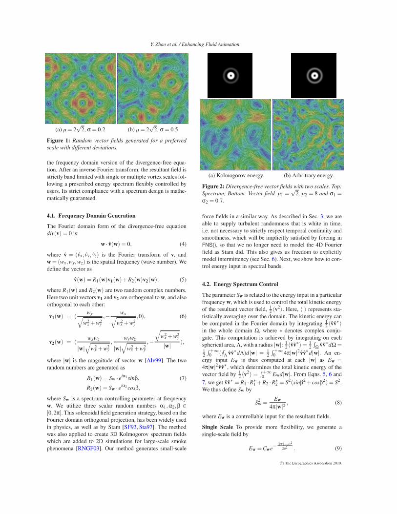
Figure 1: Random vector fields generated for a preferred

scale with different deviations.

the frequency domain version of the divergence-free equa-tion. After an inverse Fourier transform, the resultant field isstrictly band limited with single or multiple vortex scales fol-lowing a prescribed energy spectrum flexibly controlled byusers. Its strict compliance with a spectrum design is mathe-matically guaranteed.

4.1. Frequency Domain Generation

The Fourier domain form of the divergence-free equationdiv(v) = 0 is:

w · v(w) = 0, (4)

where v = (vx, vy, vz) is the Fourier transform of v, andw = (wx,wy,wz) is the spatial frequency (wave number). Wedefine the vector as

v(w) = R1(w)v1(w)+R2(w)v2(w), (5)

where R1(w) and R2(w) are two random complex numbers.Here two unit vectors v1 and v2 are orthogonal to w, and alsoorthogonal to each other:

v1(w) = (wy

√

w2x +w2

y

,− wx√

w2x +w2

y

,0), (6)

v2(w) = (wxwz

|w|√

w2x +w2

y

,wywz

|w|√

w2x +w2

y

,−

√

w2x +w2

y

|w| ),

where |w| is the magnitude of vector w [Alv99]. The tworandom numbers are generated as

R1(w) = Sw · eiα1 sinβ, (7)

R2(w) = Sw · eiα2 cosβ,

where Sw is a spectrum controlling parameter at frequencyw. We utilize three scalar random numbers α1,α2,β ∈[0,2π]. This solenoidal field generation strategy, based on theFourier domain orthogonal projection, has been widely usedin physics, as well as by Stam [SF93, Sta97]. The methodwas also applied to create 3D Kolmogorov spectrum fieldswhich are added to 2D simulations for large-scale smokephenomena [RNGF03]. Our method generates small-scale

(a) Kolmogorov energy. (b) Arbritrary energy.

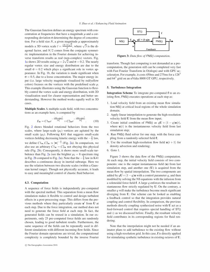
Figure 2: Divergence-free vector fields with two scales. Top:

Spectrum; Bottom: Vector field. µ1 =√

2, µ2 = 8 and σ1 =σ2 = 0.7.

force fields in a similar way. As described in Sec. 3, we areable to supply turbulent randomness that is white in time,i.e. not necessary to strictly respect temporal continuity andsmoothness, which will be implicitly satisfied by forcing inFNS(), so that we no longer need to model the 4D Fourierfield as Stam did. This also gives us freedom to explicitlymodel intermittency (see Sec. 6). Next, we show how to con-trol energy input in spectral bands.

4.2. Energy Spectrum Control

The parameter Sw is related to the energy input in a particularfrequency w, which is used to control the total kinetic energyof the resultant vector field, 1

2 〈v2〉. Here, 〈 〉 represents sta-

tistically averaging over the domain. The kinetic energy canbe computed in the Fourier domain by integrating 1

2 〈vv∗〉in the whole domain Ω, where ∗ denotes complex conju-gate. This computation is achieved by integrating on eachspherical area, Λ, with a radius |w|: 1

2 〈vv∗〉= 12

∫

Ω vv∗dΩ =12

∫ +∞0 (

∮

Λ vv∗dΛ)d|w| = 12

∫ +∞0 4π|w|2vv∗d|w|. An en-

ergy input Ew is thus computed at each |w| as Ew =4π|w|2vv∗, which determines the total kinetic energy of thevector field by 1

2 〈v2〉 =

∫ +∞0 Ewd|w|. From Eqns. 5, 6 and

7, we get vv∗ = R1 ·R∗1 +R2 ·R∗

2 = S2(sinβ2 +cosβ2) = S2.We thus define Sw by

S2w =

Ew

4π|w|2 , (8)

where Ew is a controllable input for the resultant fields.

Single Scale To provide more flexibility, we generate asingle-scale field by

Ew = Cwe− (|w|−µ)2

2σ2 . (9)

c© The Eurographics Association 2010.

Y. Zhao et al. / Enhancing Fluid Animation

The Gaussian function defines an energy spectrum with con-centration at frequencies that have a magnitude µ and a cor-responding deviation σ determining the degree of concentra-tion. For a field size N, a given magnitude µ approximately

models a 3D vortex scale l =(N/2)

√3

µ , where√

3 is the di-

agonal factor, and N/2 comes from the conjugate symmet-ric implementation in the Fourier domain for achieving in-verse transform results as real (non-complex) vectors. Fig.1a shows 2D results using µ = 2

√2 and σ = 0.2. The nearly

regular vortex size and energy distribution are due to thesmall σ = 0.2 which plays a significant role in vortex ap-pearance. In Fig. 1b, the variation is made significant whenσ = 0.5, due to a loose concentration. The major energy in-put (i.e. large velocity magnitude visualized by red/yellowcolors) focuses on the vortices with the predefined scale µ.This example illustrates using the Gaussian function to flexi-bly control the vortex scale and energy distribution, with 2Dvisualization used for clearer representation and better un-derstanding. However the method works equally well in 3Dcases.

Multiple Scales A multiple-scale field, with two concentra-tions as an example here, is computed by

Ew = C1we− (|w|−µ1)2

2σ21 +C2we

− (|w|−µ2)2

2σ22 . (10)

Fig. 2 shows blended rotational behaviors from the twoscales, where large-scale (µ1) vortices are agitated by thesmall scale (µ2). Following K41 that suggests small-scalevortices holding decreasing kinetic energy with the − 5

3 law,

we define C1w,C2w ∝ |w|− 53 (Fig. 2a). In comparison, we

also use an arbitrary C1w = C2w not obeying this physicalrule (Fig. 2b). Consequently, it shows more small-scale tur-bulence than Fig. 2a (see the brighter µ2 = 8 spectrum ringin Fig. 2b compared to Fig. 2a). Note that the − 5

3 law in K41describes a continuous decay in inertial subrange. Here weuse the relation between two discrete scales (within a Gaus-sian kernel range). Though not physically accurate, it leadsto easy and meaningful control of chaotic fluid behavior.

4.3. Computation

A sequence of force fields is independently pre-computedwith the spectral method. This separation from a mean flowsimulation makes it flexible to control and design turbulenteffects in a post-processing stage. This differs from the pre-vious methods where they particularly create u′ from U ateach step. Due to the force integration, our method does notneed to generate the force field at each step. In fact, thegenerated fields can be reused in a simulation. In our ex-periments, only 25 pre-computed force fields are randomlychosen, leading to good turbulent results. Furthermore, thesame sequence of the fields can be repeatedly used in dif-ferent simulations with different incoming flow fields. Sincethe Fourier domain operations are trivial, the computationalcomplexity is completely bounded by the inverse Fourier

NS() FNS()

ST()

U

f

u

u

qU + (1-q)u

Feedback

Figure 3: Data flow of FNS() computation.

transform. Though fast computing is not demanded as a pre-computation, the generation still can be completed very fastwith Fast Fourier Transform in O(nlogn) and with GPU ac-celeration. For example, it costs 450ms and 275ms for a 1283

and 643 grid on an nVidia 8800 GT GPU, respectively.

5. Turbulence Integration

Integration Scheme To integrate pre-computed f to an ex-isting flow, FNS() executes operations at each step as:

1. Load velocity field from an existing mean flow simula-tion NS() at critical local regions of the whole simulationdomain;

2. Apply linear interpolation to generate the high-resolutionvelocity field U from the mean flow input;

3. Create initial condition of FNS() as qU + (1 − q)u(t),where u(t) is the instantaneous velocity field from lastsimulation step;

4. Run FNS() fluid solver for one step, with the force cou-pling from a randomly-selected field f;

5. Use the resultant high-resolution flow field u(t + 1) fordensity advection and rendering;

6. Goto 1.

Figure 3 shows the data flow of the FNS() computation.At each step, the initial velocity field consists of two com-ponents: one is the output instantaneous field (u) from lastsimulation step, and another one (U) is acquired from themean flow by spatial interpolation. The two components areadded by qU+(1−q)u with a control parameter q, and thenmodified by solving the NS equations with the infusion froma solenoidal force field f. A large q enforces the resultant in-stantaneous flow strictly regulated by U. On the contrary, asmaller q will make the turbulence become much significantdiverging from U. Our scheme can be looked as enablinga feedback control so that the integration provides naturalcoupling and control flexibility. In comparison, the previousmethods directly coupling synthesized noise with U act as afeed-forward control that requires special handling of ST()

and ⊕ as we discussed before. Finally, the resultant velocityfield contributes in its corresponding regions for fluid ren-dering.

Note that the interpolation might not be needed if an an-imator plans to add turbulence to the existing flow withoutusing a high-resolution grid. In this case, f is directly appliedfor stimulating synthetic turbulence in existing octaves of U.

c© The Eurographics Association 2010.

Y. Zhao et al. / Enhancing Fluid Animation

Besides the Eulerian solver, our method can also be di-rectly applied to Lagrangian fluid solvers. We conduct an ex-periment with the state-of-the-art SPH methods (SmoothedParticle Hydrodynamics), which have been widely exploredin computer graphics due to its programming simplic-ity, various simulation scales and easy boundary handling[MCG03]. Together with the typical pressure and viscos-ity forces, we impose f to each particle, manifesting theunsolved turbulent behavior. The force coupling strategyhas no difference from Eulerian approaches, which is de-scribed below. To the best of our knowledge, this is the firsttime in graphics applying turbulence enhancement to a pureLagrangian solver (Note that though with introduced vor-tex particles, [PTSG09] still relies mainly on an Euleriansolver).

Force Coupling A stochastic force f should perform in theturbulence simulator with respect to the mean flow proper-ties. We match the force f with U at each location, usingthe graphical assumption B as in previous works (see Sec.1). At first, we make f ·U ≤ 0 by reversing the direction off if needed. This guarantees the randomly created turbulentfluctuation will not reverse U dramatically that leads to un-natural flow variation effects. Second, we follow the magni-tude relation |f| ∝ |uf|/δt [OP98], where δt is the turbulencesimulation time step length and uf is the introduced velocityvariation by f. Finally an amplitude relation between uf andU should be determined: |uf|= pc|U|, where pc is a couplingparameter. Then we achieve

|f| = |uf|/δt = pc|U|/δt. (11)

pc can be found by applying the velocity cascade relationamong octaves of uf and U [KTJG08]. This approach is fea-sible but increases complexity. It indeed may not be nec-essary due to the approximation already produced by thegraphical assumptions. pc can be more conveniently definedas an empirical control parameter. In general, if a function isdefined as |f|= Ψ(U), Ψ provides a very good tool to controlthe turbulence integration, and hence the final fluid effects.Besides Eqn. 11, we describe flexible approaches of Ψ inSec. 6.

6. Conditional and Intermittent Turbulence

Forcing acts as a stimulus for inducing chaotic effects ratherthan adding a resultant turbulent field to global flow, leadingto easy implementation of (1) adaptive turbulence only innecessary spatial areas and temporal periods; and (2) con-ditional turbulent effects with physical or artificial condi-tions. We apply turbulence forcing within critical areas ina large domain running global simulation. The turbulent ef-fects will propagate out of the selected local regions throughthe motion of scalar densities. This approach is very usefulfor many applications such as interactive games and emer-gency training.

Conditional Coupling As discussed in Sec. 5, a function Ψ

is to determine the integration conditions of turbulence. Wehave defined Eqn. 11, which couples turbulence in the wholeeffective region based on velocity magnitude. Here we pro-vide several other choices for different animation purposes:

• Strain rate: At each location r, the local strain rateS(U)2 = ∑∑((∂Ui/∂r j +∂U j/∂ri)/2)2. We define

|f| = Ψ(U) = pc|w1|−1S(U)/δt, (12)

so that turbulence is initiated at locations with a large rateof change in U.

• Distance: Obstacles are prone to introduce high strain ratethus causing boundary-induced turbulence. While smallobstacles may not be fully accounted for in a coarse gridsimulation of U, a fluid animation can define

|f| = Ψ(U) = pcRamp(D(r)

D0)|U|/δt, (13)

where D(r) is the shortest distance from r to the obstaclesand D0 is a cutting length. Ramp() defines a smoothly de-creasing function from one to zero for D(r) < D0, andotherwise it equals zero. Here we link D(r) to boundarylayer effects, based on an observation that the profile ofshear stress, which leads to turbulence, is a decreasingcurve of the distance to the boundary surface [Pop00].

• Vorticity: Similar to strain rate, turbulence is related tothe vorticity by

|f| = Ψ(U) = pc|ω|

max(|ω|) H(|ω|− |ω|0)/δt, (14)

where the vorticity ω = ∇×U, H() is the Heaviside stepfunction, and |ω|0 is a threshold used to control the effectstogether with pc.

• Density: Turbulence can be triggered by a function of thescalar density m of fluid. A simple formula is

|f| = Ψ(U) = pcm

max(m)H(m−m0)|U|/δt, (15)

where H() is the Heaviside function and m0 is a threshold.

These examples illustrate that our solution supplies a frame-work incorporating a variety of turbulence starters, fromphysical features to an animator’s discretion, which can befurther improved and extended for controllable and interac-tive animations.

Intermittency Turbulent fluids show alternations in timebetween nearly non-turbulent and chaotic behavior, whichchallenges K41’s hypothesis of universality. Many attempts,including by Kolmogorov himself, have been proposed toexplain and solve the problem. It is extremely hard to presentintermittency physically by DNS. We instead introduce tem-poral control in forcing integration to animate intermit-tent fluids. The fluid behaves in non-turbulent or turbulentdynamics alternately with randomly varied time intervals,∆tturb and ∆tnon, respectively. We initiate turbulence cou-pling in intervals of ∆tturb, and otherwise use the large-scale flow only. The two intervals are computed, when each

c© The Eurographics Association 2010.

Y. Zhao et al. / Enhancing Fluid Animation

(a) (b) (c) (d)

(e) (f) (g) (h)

Figure 4: Snapshots of turbulence enhancement simulations: (a) Original coarse simulation; (b) Wavelet subgrid turbulence;

(c) Our subgrid turbulence; (d) Add vorticity confinement to (a); (e) Wavelet turbulence to (d); (f) Our turbulence to (d) with

q = 0.8; (g) Our turbulence to (d) with q = 0.2; (h) Our turbulence to (d) with q = 0.1.

time needed, as scalar random values by ∆tturb ∈ [0,Lturb]and ∆tnon ∈ [0,Lnon], where Lturb and Lnon are used to con-trol the maximum interval length in time steps. However,when sometimes ∆tnon = 0, two turbulent periods are con-catenated. For the whole animation period, the intermittencyfactor is γ = Σ(∆tturb)/Σ(∆tturb +∆tnon).

7. Experiments

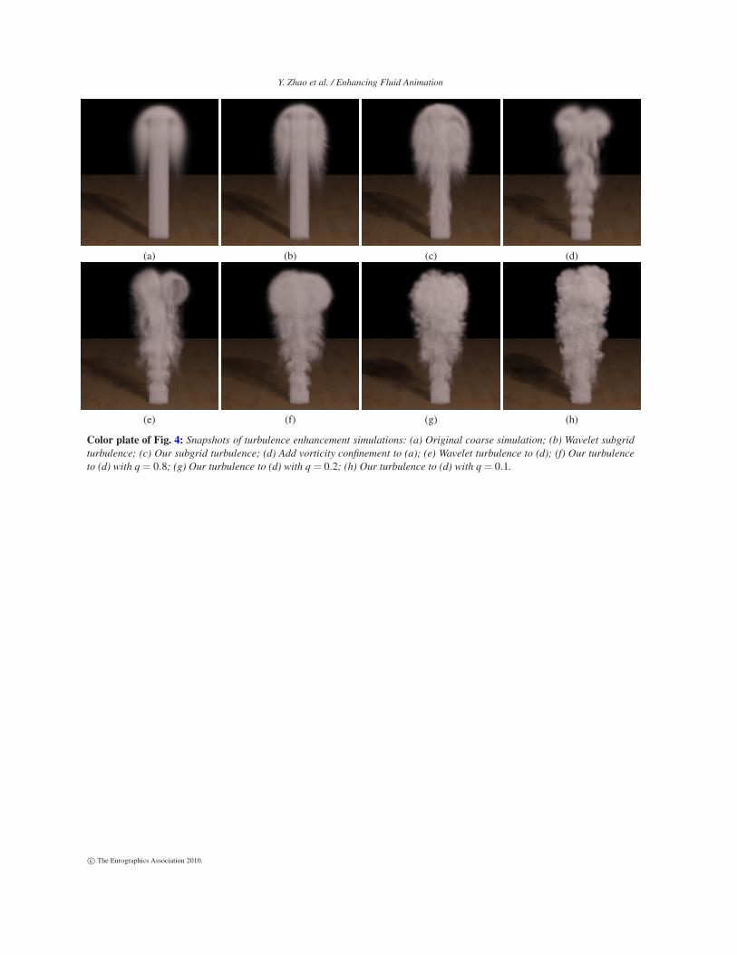
Exp. 1 First, we describe our method in Fig. 4 in com-parison to the successful wavelet turbulence enhancementmethod [KTJG08]. A basic stable solver [Sta99] generatesvery static smoke effects with a coarse 48× 64× 48 simu-lation (Fig. 4a). Wavelet turbulence adds subgrid turbulencewith a 2x finer grid (Fig. 4b). Our method creates similarsubgrid turbulence in Fig. 4c with µ = 32

√3 and pc = 0.5.

Our solution looks relatively more realistic since the forc-ing can impose chaotic behavior even for this very regularmean flow, while the wavelet approach’s effect is contin-gent on the original U. We then add the vorticity confine-ment [FSJ01] to Fig. 4a producing large-scale rotational be-havior (Fig. 4d). In this case, the wavelet turbulence pro-vides good small-scale turbulence (Fig. 4e). In comparison,our method can introduce small-scale turbulence in differentlevels with the control parameter q (see Fig. 3). In Fig. 4f,with q = 0.8 mainly supplying the mean flow component to

FNS(), the enhanced smoke propagates close to the originshape of Fig. 4d which is similar to the wavelet result. Whilewe decrease q = 0.2, turbulence becomes significant in Fig.4g since more enhanced component feedbacks to FNS() in-ducing amplification effects. In Fig. 4h, q = 0.1 leads to evenstronger turbulent effects. On a PC CPU (Intel Core2 63001.86GHz 4GB), our turbulent enhancement runs in 12982ms per step, and the wavelet method uses 4048 ms per step,respectively. We compare these animations side by side inthe supplemental movie to illustrate the dynamic difference.

Exp. 2 Next, we execute our animation using q = 0.2 basedon a simulated laminar smoke past a sphere with a verycoarse grid at 16×32×16. To better illustrate our approach,no enhancing techniques (e.g. vorticity confinement) are em-ployed. We use a smoke evolving grid with a resolution4x denser at 64 × 128 × 64. Turbulence integration is im-plemented on a local region surrounding the sphere witha resolution 38 × 76 × 38. Fig. 5 shows snapshots of theintegrated turbulence at different scales: (a) original lami-nar result; (b) small turbulent variation with a subgrid scale(µsub = 16

√3) that approximates the grid scaling factor 4

(pc = 0.3); (c) strong turbulent dynamics with a larger scale(µl = 1

3 µsub, pc = 0.5); (d) turbulent behavior accommodat-ing finer details than (c), with two coalesced scales (µl andµsub) following − 5

3 law (pc = 0.5); (e) reproducing dynam-ics of (d) with an arbitrary spectrum law where two octaves

c© The Eurographics Association 2010.

Y. Zhao et al. / Enhancing Fluid Animation

(a) Original fluid (b) Subgrid scale turbulence (c) Large scale turbulence

(d) Multiple scale turbulence (K41) (e) Multiple scale turbulence (Arbitrary) (f) Density based turbulence

Figure 5: Snapshots of integrating turbulence to a laminar smoke.

(µl and µsub) having an equalized energy spectrum (non-Kolmogorov), which further reduces the effects of the largescale one. Fig. 5b-e use Eqn. 11 for force integration. Finallyin Fig. 5f smoke density (Eqn. 15) is used to trigger turbu-lence. We use σ = 0.5 for the simulations. In the supple-mental movie, we compare the smoke effects in the differentconfigurations. We also include multiscale animations usingthe vorticity (Eqn. 14) and strain rate (Eqn. 12) based turbu-lence integration, where chaotic variations appear around thesphere. On the PC CPU, the experiment uses 48 ms per stepfor the global simulation and 956 ms per step for the inter-polation, integration and forced simulation. The density ad-vection costs 342 ms. In comparison, a direct 64× 128× 64simulation consumes 8715 ms that is 6.5 times slower, whichcannot generate the various turbulent results.

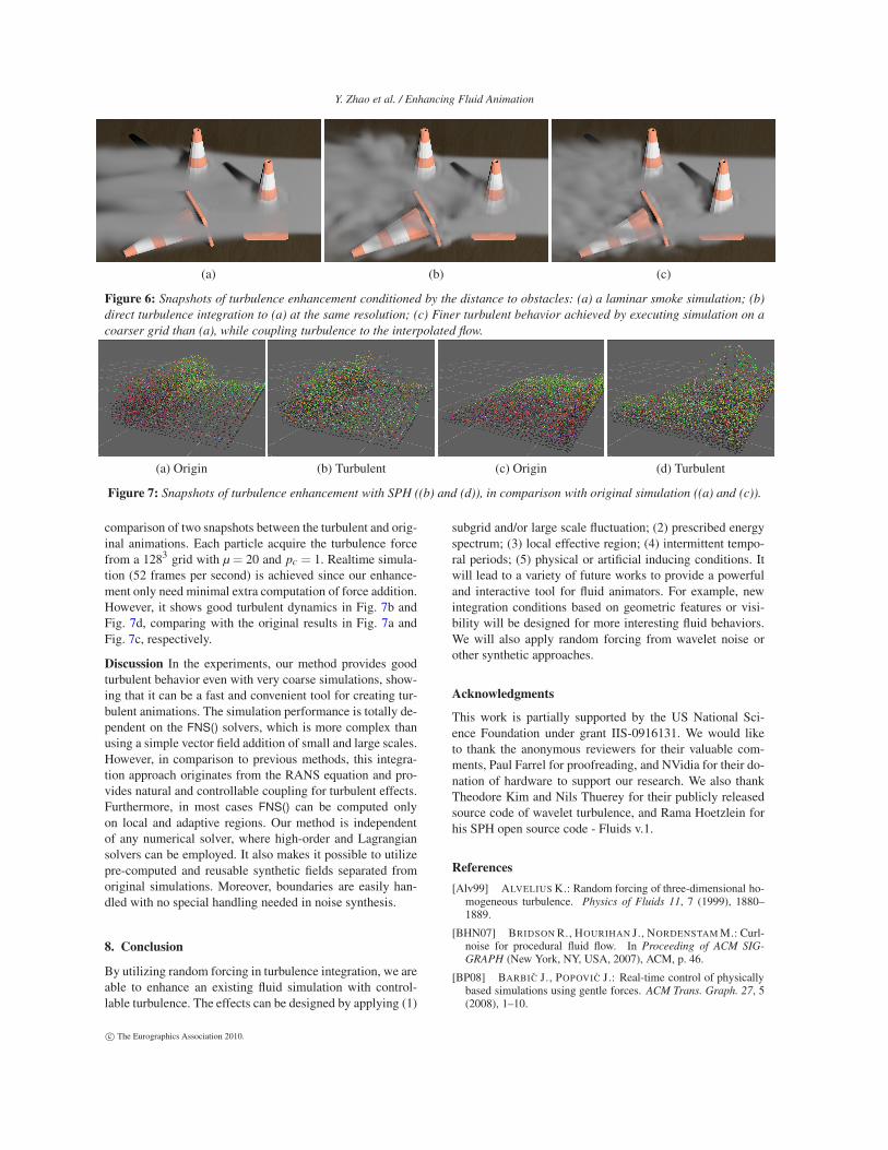
Exp. 3 Another experiment is applied with three obstaclesusing q = 0.2, as shown in Fig. 6. Here we utilize the dis-tance based turbulence enhancement condition (Eqn. 13) to

approximate boundary induced chaos. Fig. 6a is the origi-nal simulation result with a resolution 64× 32× 50. Fig. 6bpresents a turbulent flow by adding turbulence forces to Fig.6a without any interpolation or subgrid time steps. We useµ = 12

√3, σ = 0.7 and pc = 0.5. The 64× 32× 50 simula-

tion (with or without turbulence) runs in 628 ms per frameon the PC CPU and the added force does not increase no-ticeable computing overload. In Fig. 6c, we instead run theglobal simulation on a 2x coarser grid at 32×16×25 (51 msper frame), and apply turbulence integration on an interpo-lated grid at 64× 32× 50. It shows finer turbulent featurescompared with Fig. 6b using a larger µ = 16

√3. With this

configuration, we also include intermittent turbulent effectsin the supplemental movie using Lturb = 20 and Lnon = 40steps.

Exp. 4 We also perform SPH based turbulence enhancement.We use 4096 particles to perform a wave simulation. We fol-low [MCG03] for implementation details. Fig. 7 shows the

c© The Eurographics Association 2010.

Y. Zhao et al. / Enhancing Fluid Animation

(a) (b) (c)

Figure 6: Snapshots of turbulence enhancement conditioned by the distance to obstacles: (a) a laminar smoke simulation; (b)

direct turbulence integration to (a) at the same resolution; (c) Finer turbulent behavior achieved by executing simulation on a

coarser grid than (a), while coupling turbulence to the interpolated flow.

(a) Origin (b) Turbulent (c) Origin (d) Turbulent

Figure 7: Snapshots of turbulence enhancement with SPH ((b) and (d)), in comparison with original simulation ((a) and (c)).

comparison of two snapshots between the turbulent and orig-inal animations. Each particle acquire the turbulence forcefrom a 1283 grid with µ = 20 and pc = 1. Realtime simula-tion (52 frames per second) is achieved since our enhance-ment only need minimal extra computation of force addition.However, it shows good turbulent dynamics in Fig. 7b andFig. 7d, comparing with the original results in Fig. 7a andFig. 7c, respectively.

Discussion In the experiments, our method provides goodturbulent behavior even with very coarse simulations, show-ing that it can be a fast and convenient tool for creating tur-bulent animations. The simulation performance is totally de-pendent on the FNS() solvers, which is more complex thanusing a simple vector field addition of small and large scales.However, in comparison to previous methods, this integra-tion approach originates from the RANS equation and pro-vides natural and controllable coupling for turbulent effects.Furthermore, in most cases FNS() can be computed onlyon local and adaptive regions. Our method is independentof any numerical solver, where high-order and Lagrangiansolvers can be employed. It also makes it possible to utilizepre-computed and reusable synthetic fields separated fromoriginal simulations. Moreover, boundaries are easily han-dled with no special handling needed in noise synthesis.

8. Conclusion

By utilizing random forcing in turbulence integration, we areable to enhance an existing fluid simulation with control-lable turbulence. The effects can be designed by applying (1)

subgrid and/or large scale fluctuation; (2) prescribed energyspectrum; (3) local effective region; (4) intermittent tempo-ral periods; (5) physical or artificial inducing conditions. Itwill lead to a variety of future works to provide a powerfuland interactive tool for fluid animators. For example, newintegration conditions based on geometric features or visi-bility will be designed for more interesting fluid behaviors.We will also apply random forcing from wavelet noise orother synthetic approaches.

Acknowledgments

This work is partially supported by the US National Sci-ence Foundation under grant IIS-0916131. We would liketo thank the anonymous reviewers for their valuable com-ments, Paul Farrel for proofreading, and NVidia for their do-nation of hardware to support our research. We also thankTheodore Kim and Nils Thuerey for their publicly releasedsource code of wavelet turbulence, and Rama Hoetzlein forhis SPH open source code - Fluids v.1.

References

[Alv99] ALVELIUS K.: Random forcing of three-dimensional ho-mogeneous turbulence. Physics of Fluids 11, 7 (1999), 1880–1889.

[BHN07] BRIDSON R., HOURIHAN J., NORDENSTAM M.: Curl-noise for procedural fluid flow. In Proceeding of ACM SIG-

GRAPH (New York, NY, USA, 2007), ACM, p. 46.

[BP08] BARBIC J., POPOVIC J.: Real-time control of physicallybased simulations using gentle forces. ACM Trans. Graph. 27, 5(2008), 1–10.

c© The Eurographics Association 2010.

Y. Zhao et al. / Enhancing Fluid Animation

[Bri08] BRIDSON R.: Fluid Simulation for Computer Graphics.A. K. Peters, Ltd., Natick, MA, USA, 2008.

[CD96] CANUTO V., DUBOVIKOV M.: A dynamical model forturbulence. i. general formalism. Physics of Fluids 8, 2 (1996).

[ETK∗07] ELCOTT S., TONG Y., KANSO E., SCHRÖDER P.,DESBRUN M.: Stable, circulation-preserving, simplicial fluids.ACM Trans. Graph. 26, 1 (2007), 4.

[FL04] FATTAL R., LISCHINSKI D.: Target-driven smoke anima-tion. In SIGGRAPH ’04: ACM SIGGRAPH 2004 Papers (NewYork, NY, USA, 2004), ACM, pp. 441–448.

[Fri95] FRISCH U.: Turbulence: The legacy of A.N. Kolmogorov.Cambridge University Press, 1995.

[FSJ01] FEDKIW R., STAM J., JENSEN H.: Visual simulation ofsmoke. Proceedings of SIGGRAPH (2001), 15–22.

[KLLR07] KIM B., LIU Y., LLAMAS I., ROSSIGNAC J.: Ad-vections with significantly reduced dissipation and diffusion.IEEE Transactions on Visualization and Computer Graphics 13,1 (2007), 135–144.

[KTJG08] KIM T., THÜREY N., JAMES D., GROSS M.: Waveletturbulence for fluid simulation. In Proceeding of ACM SIG-GRAPH (New York, NY, USA, 2008), ACM, pp. 1–6.

[LDM03] LAVAL J., DUBRULLE B., MCWILLIAMS J. C.:Langevin models of turbulence: Renormalization group, distantinteraction algorithms or rapid distortion theory? Physics Of Flu-

ids 15, 5 (2003).

[LGF04] LOSASSO F., GIBOU F., FEDKIW R.: Simulating waterand smoke with an octree data structure. ACM Trans. Graph. 23,3 (2004), 457–462.

[MCG03] MÜLLER M., CHARYPAR D., GROSS M.: Particle-based fluid simulation for interactive applications. In Proceed-

ings of the ACM SIGGRAPH/Eurographics symposium on Com-puter animation (Aire-la-Ville, Switzerland, Switzerland, 2003),Eurographics Association, pp. 154–159.

[MCP∗09] MULLEN P., CRANE K., PAVLOV D., TONG Y.,DESBRUN M.: Energy-preserving integrators for fluid anima-tion. ACM Trans. Graph. 28, 3 (2009).

[NSCL08] NARAIN R., SEWALL J., CARLSON M., LIN M. C.:Fast animation of turbulence using energy transport and proce-dural synthesis. In Proceeding of ACM SIGGRAPH Asia (NewYork, NY, USA, 2008), ACM, pp. 1–8.

[OP98] OVERHOLT M. R., POPE S. B.: A deterministic forcingscheme for direct numerical simulations of turbulence. Comput.Fluids 27, 1 (1998), 11–28.

[PN01] PERLIN K., NEYRET F.: Flow noise. ACM SIGGRAPH

Technical Sketches and Applications (2001), 187.

[Pop00] POPE S. B.: Turbulent Flows. Cambridge UniversityPress, 2000.

[PT05] PATEL M., TAYLOR N.: Simple divergence-free fields forartistic simulation. Journal of Graphics Tools 10, 4 (2005), 49–60.

[PTSG09] PFAFF T., THUEREY N., SELLE A., GROSS M.: Syn-thetic turbulence using artificial boundary layers. In SIGGRAPH

Asia ’09: ACM SIGGRAPH Asia 2009 papers (New York, NY,USA, 2009), ACM, pp. 1–10.

[RNGF03] RASMUSSEN N., NGUYEN D. Q., GEIGER W., FED-KIW R.: Smoke simulation for large scale phenomena. ACM

Trans. Graph. 22, 3 (2003), 703–707.

[SB08] SCHECHTER H., BRIDSON R.: Evolving sub-grid turbu-lence for smoke animation. In Eurographics/ACM SIGGRAPH

Symposium on Computer Animation (2008), pp. 1–8.

[SF93] STAM J., FIUME E.: Turbulent wind fields for gaseousphenomena. In Proceeding of ACM SIGGRAPH (New York, NY,USA, 1993), ACM, pp. 369–376.

[SRF05] SELLE A., RASMUSSEN N., FEDKIW R.: A vortex par-ticle method for smoke, water and explosions. Proceedings of

SIGGRAPH (2005), 910–914.

[Sta97] STAM J.: A general animation framework for gaseousphenomena. ERCIM Research Report R047 (1997).

[Sta99] STAM J.: Stable fluids. In Proceeding of ACM SIG-

GRAPH (New York, NY, USA, 1999), ACM Press, pp. 121–128.

[SY05] SHI L., YU Y.: Controllable smoke animation with guid-ing objects. ACM Trans. Graph. 24, 1 (2005), 140–164.

[TKPR06] THÜREY N., KEISER R., PAULY M., RÜDE U.:Detail-preserving fluid control. In Proceedings of the 2006 ACM

SIGGRAPH/Eurographics symposium on Computer animation

(Aire-la-Ville, Switzerland, Switzerland, 2006), pp. 7–12.

[Vos85] VOSS R. F.: Random fractal forgeries. In FundamentalAlgorithms in Computer Graphics, Earnshaw R., (Ed.). Springer,1985, pp. 805–883.

[WST09] WICKE M., STANTON M., TREUILLE A.: Modularbases for fluid dynamics. ACM Trans. Graph. 28, 3 (2009), 1–8.

[ZB05] ZHU Y., BRIDSON R.: Animating sand as a fluid. InProceedings of ACM SIGGRAPH (New York, NY, USA, 2005),ACM, pp. 965–972.

c© The Eurographics Association 2010.

Y. Zhao et al. / Enhancing Fluid Animation

(a) (b) (c) (d)

(e) (f) (g) (h)

Color plate of Fig. 4: Snapshots of turbulence enhancement simulations: (a) Original coarse simulation; (b) Wavelet subgrid

turbulence; (c) Our subgrid turbulence; (d) Add vorticity confinement to (a); (e) Wavelet turbulence to (d); (f) Our turbulence

to (d) with q = 0.8; (g) Our turbulence to (d) with q = 0.2; (h) Our turbulence to (d) with q = 0.1.

c© The Eurographics Association 2010.