Enhancing Associative Memory Recall and Storage Capacity ...

Enhancing Associative Memory Recall and Storage Capacity Using Confocal Cavity QED

Brendan P. Marsh ,1,2 Yudan Guo,2,3 Ronen M. Kroeze,2,3 Sarang Gopalakrishnan,4

Surya Ganguli,1 Jonathan Keeling ,5 and Benjamin L. Lev1,2,31Department of Applied Physics, Stanford University, Stanford, California 94305, USA

2E. L. Ginzton Laboratory, Stanford University, Stanford, California 94305, USA3Department of Physics, Stanford University, Stanford, California 94305, USA

4Department of Engineering Science and Physics, CUNY College of Staten Island,Staten Island, New York 10314, USA

5SUPA, School of Physics and Astronomy, University of St. Andrews,St. Andrews KY16 9SS, United Kingdom

(Received 4 September 2020; revised 3 April 2021; accepted 28 April 2021; published 2 June 2021)

We introduce a near-term experimental platform for realizing an associative memory. It cansimultaneously store many memories by using spinful bosons coupled to a degenerate multimode opticalcavity. The associative memory is realized by a confocal cavity QED neural network, with the modesserving as the synapses, connecting a network of superradiant atomic spin ensembles,which serve as theneurons. Memories are encoded in the connectivity matrix between the spins and can be accessed throughthe input and output of patterns of light. Each aspect of the scheme is based on recently demonstratedtechnology using a confocal cavity and Bose-condensed atoms. Our scheme has two conceptually novelelements. First, it introduces a new form of random spin system that interpolates between a ferromagneticand a spin glass regime as a physical parameter is tuned—the positions of ensembles within the cavity.Second, and more importantly, the spins relax via deterministic steepest-descent dynamics rather thanGlauber dynamics. We show that this nonequilibrium quantum-optical scheme has significant advantagesfor associative memory over Glauber dynamics: These dynamics can enhance the network’s ability to storeand recall memories beyond that of the standard Hopfield model. Surprisingly, the cavity QED dynamicscan retrieve memories even when the system is in the spin glass phase. Thus, the experimental platformprovides a novel physical instantiation of associative memories and spin glasses as well as provides anunusual form of relaxational dynamics that is conducive to memory recall even in regimes where it wasthought to be impossible.

DOI: 10.1103/PhysRevX.11.021048 Subject Areas: Atomic and Molecular Physics,Quantum Physics, Statistical Physics

I. INTRODUCTION

Five hundred million years of vertebrate brain evolutionhave produced biological information-processing architec-tures so powerful that simply emulating them, in the formof artificial neural networks, has led to breakthroughs inclassical computing [1,2]. Indeed, neuromorphic compu-tation currently achieves state-of-the-art performance inimage and speech recognition and machine translation andeven outperforms the best humans in complex games likeGo [3]. Meanwhile, a revolution in our ability to controland harness the quantum world is promising technological

breakthroughs for quantum information processing [4,5]and sensing [6]. Thus, combining the algorithmic principlesof robust parallel neural computation, discovered bybiological evolution, with the nontrivial quantum dynamicsof interacting light and matter naturally offered to us by thephysical world may open up a new design space ofquantum-optics-based neural networks. Such networkscould potentially achieve computational feats beyond any-thing biological or silicon-based machines could do alone.We present an initial step along this path by theoretically

showing how a network composed of atomic spins coupledby photons in a multimode cavity can naturally realizeassociative memory, which is a prototypical brainlikefunction of neural networks. Moreover, we find that,including the effects of drive and dissipation, the naturallyarising nonequilibrium dynamics of the cavity QED systemenhances its ability to store and recall multiple memorypatterns, even in a spin glass phase.

Published by the American Physical Society under the terms ofthe Creative Commons Attribution 4.0 International license.Further distribution of this work must maintain attribution tothe author(s) and the published article’s title, journal citation,and DOI.

PHYSICAL REVIEW X 11, 021048 (2021)Featured in Physics

2160-3308=21=11(2)=021048(39) 021048-1 Published by the American Physical Society

https://orcid.org/0000-0002-8451-4425

https://orcid.org/0000-0002-4283-552X

https://crossmark.crossref.org/dialog/?doi=10.1103/PhysRevX.11.021048&domain=pdf&date_stamp=2021-06-02

https://doi.org/10.1103/PhysRevX.11.021048




https://creativecommons.org/licenses/by/4.0/

https://creativecommons.org/licenses/by/4.0/

Despite the biologically inspired name, artificial neuralnetworks can refer to any network of nonlinear elements(e.g., spins) whose state depends on signals (e.g., magneticfields) received from other elements [7–9]. They provide adistributed computational architecture alternative to thesequential gate-based von Neumann model of computingwidely used in everyday devices [10] and employed intraditional quantum computing schemes [4]. Rather thanbeing programmed as a sequence of operations, the neural-network connectivity encodes the problem to be solved as acost function, and the solution corresponds to the finalsteady-state configuration obtained by minimizing this costfunction through a nonlinear dynamical evolution of theindividual elements. Specifically, the random, frustratedIsing spin glass is an archetypal mathematical setting forexploring neural networks [7]. Finding the ground state ofan Ising spin glass is known to be an NP-hard problem[11,12], and so different choices of the spin connectivitymay, therefore, encode many different combinatorial opti-mization problems of broad technological relevance[13,14]. Much of the excitement in modern technologicaland scientific computing revolves around developing faster,more efficient “heuristic” optimization solvers that provide“good-enough” solutions. Physical systems capable ofrealizing an Ising spin glass may play such a role. In thisspirit, we present a thorough theoretical investigation of aquantum-optics-based heuristic neural-network optimiza-tion solver in the context of the associative memoryproblem.Using notions from statistical mechanics, Hopfield

showed how a spin glass of randomly connected Isingspins can be capable of associative memory [15].Associative memory is able to store multiple patterns(memories) as local minima of an energy landscape.Moreover, recall of any individual memory is possibleeven if mistakes are made when addressing the memory tobe recalled: If the network is initialized by an externalstimulus in a state that is not too different from the storedmemory, then the network dynamics will flow toward aninternal representation of the original stored memory, usingan energy-minimizing process called pattern completionthat corrects errors in the initial state. Such networks exhibita trade-off between capacity (number of memories stored)and robustness (the size of the basins of attraction of eachmemory under pattern completion). Once too many memo-ries are stored, the basins of attraction cease to be extensive,and the model transitions to a spin glass regime withexponentially many spurious memories (with subextensivebasins of attraction) that are nowhere near the desiredmemories [16]. Intriguingly, Hopfield-like associativememories have resurfaced recently at the frontiers ofpractical machine learning and are shown to be closelyrelated [17] to transformer networks underlying manyadvances in natural language processing, machine vision,and protein folding.

From a hardware perspective, most modern neural net-works are implemented in complementary metal oxidesemiconductor devices based on electronic von Neumannarchitectures. In contrast, early work aiming to useclassical, optics-based spin representations sought to takeadvantage of the natural parallelism of light propagation[18–20]; such work continues in the context of siliconphotonic integrated circuits and other coupled classicaloscillator systems [21,22]. The use of atomic spins coupledvia light promises additional advantages: Atom-photoninteractions can be strong even on the single-photon level[23], providing the ability to process small signals andexploit manifestly quantum effects and dynamics.Previous theoretical work sketched how a spin glass and

neural network may be realized using ultracold atomsstrongly coupled via photons confined within a multimodeoptical cavity [24,25]. The cavity modes serve as thesynaptic connections of the network, mediating Isingcouplings between atomic spins. The arrangement of atomswithin the cavity determines the specific connectionstrengths of the network, which, in turn, determine thestored patterns. The atoms may be reproducibly trapped ina given connectivity configuration using optical tweezerarrays [26,27]. Subsequent studies provide additionaltheory support to the notion that related quantum-opticalsystems can implement neural networks [28–33]. However,all these works, including Refs. [24,25], leave significantaspects of implementation and capability unexplored.In the present theoretical study, we introduce the first

practicable scheme for a quantum-optical associativememory by explicitly treating photonic dissipation andensuring that the physical system does indeed behavesimilarly to a Hopfield neural network. All physicalresources invoked in this treatment are demonstrated inrecent experiments [34–40]. Specifically, we show thatsuitable network connectivity is provided by optical pho-tons in the confocal cavity, a type of degenerate multimoderesonator [41]. The photons are scattered into the cavityfrom atoms pumped by a coherent field oriented transverseto the cavity axis, as illustrated in Fig. 1. The atomsundergo a transition to a superradiant state above a thresh-old in pump strength. In this state, the spins effectivelyrealize a system of rigid (easy-axis) Ising spins with rapidspin evolution, ensuring that memory retrieval can takeplace before heating by spontaneous emission can play adetrimental role. We, moreover, find the cavity QEDsystem naturally leads to a discrete analog of “steepestdescent” dynamics, which we show provides an enhancedmemory capacity compared to standard Glauber dynamics[42]. Finally, the spin configuration can be read out byholographic imaging of the emitted cavity light, as recentlydemonstrated [38]. That is, the degenerate cavity provideshigh-numerical-aperture spatial resolving capability andmay be construed as an active quantum gas microscope, in

BRENDAN P. MARSH et al. PHYS. REV. X 11, 021048 (2021)

021048-2

analogy to apparatuses employing high-numerical-aperturelenses near optically trapped atoms [43].Our main results are as follows.(1) Superradiant scattering of photons by sufficiently

large ensembles of atomic spins plus cavity dissipa-tion naturally realizes a form of zero-temperaturedynamics in a physical setting: discrete steepestdescent (SD) dynamics. This dynamics occursbecause the bath structure dictates that largeenergy-lowering spin flips occur most rapidly. Thisenergy-lowering dynamics arises because, for largeensembles, the low-energy effective temperature issignificantly smaller than the typical ensemble spin-flip energy. This dynamics is distinct from the typicalzero-temperature limit of Glauber [42] or zero-temperature Metropolis-Hastings (0TMH) [44,45]dynamics typically considered in Hopfield neuralnetworks [46].

(2) The confocal cavity can naturally provide a dense(all-to-all) spin-spin connectivity that is tunablebetween (i) a ferromagnetic regime, (ii) a regimewith many large basins of attraction suitable forassociative memory, and (iii) a regime in which theconnectivity describes a Sherrington-Kirkpatrick(SK) spin glass. This sequence of regimes is char-acteristic of Hopfield model behavior.

(3) Surprisingly, standard limits on memory capacityand robustness are exceeded under SD dynamics.This enhancement is because SD dynamics enlargethe basins of attraction—i.e., 0TMH can lead toerrant fixed points in regimes where SD always leadsto the correct one. This result is true not just of thecavity QED system, but also for the basic Hopfieldmodel with Hebbian and other learning rules. More-over, the enhancement persists into the SK spin glass

regime, wherein basins of metastable states expandfrom zero size under 0TMH dynamics to an exten-sively scaling size under SD.

(4) While simulating the SD dynamics requires OðN2Þnumerical operations to determine the optimalenergy-lowering spin flip, the physical cavityQED system naturally flips the optimal spin dueto the different rates experienced by different spins.Thus, the real dynamics drives the spins to convergeto a fixed point configuration (memory) moreefficiently than numerical SD or 0TMH dynamics,assuming similar spin-flip rates.

(5) We introduce a pattern storage method that allowsone to program associative memories in the cavityQED system. The memory capacity of the cavityunder this scheme can be as large as N patterns.Encoding states requires only a linear transformationand a threshold operation on the input and outputfields, which can be implemented in an opticalsetting via spatial light modulators. While thestandard Hopfield model does not require encoding,it cannot naturally be realized in a multimode cavityQED system. Thus, the physical cavity QED systemenjoys roughly an order-of-magnitude greatermemory capacity at the expense of an encoder.

(6) Overall, our storage and recall scheme points to anovel paradigm for memory systems in which newstimuli are remembered by translating them intoalready intrinsically stable emergent patterns of thenative network dynamics.

The remainder of this paper is organized as follows. Wefirst describe the physical confocal cavity QED (CCQED)system in Sec. II before introducing the Hopfield model inSec. III. Next, we analyze the regimes of spin-spinconnectivity provided by the confocal cavity in Sec. IV.We then discuss in Sec. V the SD dynamics manifest in atransversely pumped confocal cavity above the superra-diant transition threshold. Section VI discusses how SDdynamics enhances associative memory capacity androbustness. A learning rule that maps free-space lightpatterns into stored memory is presented in Sec. VII.Last, in Sec. VIII, we conclude and frame our work in a

wider context. In this discussion, we speculate about howthe quantum dynamics of the superradiant transition mightenhance solution finding. All elsewhere in this paper, weconsider only the semiclassical regime well above thetransition itself. Embedding neural networks in systemsemploying ion traps, optical lattices, and optical-parametricoscillators has been explored [47–50], and comparisons ofthe latter to our scheme is discussed here also. This sectionalso provides concluding remarks regarding how thestudy of this physical system may provide new perspectiveson the problem of how memory arises in biologicalsystems [51].

FIG. 1. Sketch of the confocal cavity QED system with atomicspin ensembles confined by optical tweezers. Shown are thecavity mirrors (gray), superpositions of the cavity modes (blue),Bose-Einstein condensates (BECs) (red), optical tweezer beams(green), transverse pump beam (red), and interference on acharge-coupled device (CCD) camera for holographic imagingof spin states.

ENHANCING ASSOCIATIVE MEMORY RECALL AND STORAGE … PHYS. REV. X 11, 021048 (2021)

021048-3

Appendixes A–F present the following: Appendix A, theRaman coupling scheme and effective Hamiltonian;Appendix B, the derivation of the confocal connectivity;Appendix C, the derivation of the confocal connectivityprobability distribution; Appendix D, the spin-flip dynam-ics in the presence of a classical bath with an Ohmic noisespectrum; Appendix E, the derivation of the spin-flip rateand dynamics in the presence of a quantum bath; andAppendix F, the derivation of the mean-field ensembledynamics.

II. CONFOCAL CAVITY QED

As illustrated in Fig. 1, we consider a configuration of Nspatially separated Bose-Einstein condensates (BECs)placed in a confocal cavity. In a confocal cavity, the cavitylength L is equal to the radius of the curvature of themirrors R, which leads to degenerate optical modes [41].More specifically, modes form degenerate families, whereeach family consists of a complete set of transverseelectromagnetic TEMlm modes with lþm either of evenor odd parity. Recent experiments demonstrate couplingbetween compactly confined BECs of ultracold 87Rb atomsand a high-finesse, multimode (confocal) optical cavitywith L ¼ R ¼ 1 cm [34–39].The coupling between the BECs and the cavity occurs

via a double Raman pumping scheme illustrated in Fig. 2.The jF;mFi ¼ j1;−1i and j2;−2i states are coupled viatwo-photon processes, involving pump lasers orientedtransverse to the cavity axis and the cavity fields [52].The motion of atoms may be suppressed by introducing adeep 3D optical lattice into the cavity [53]. When atoms arethus trapped, each BEC can be described as an ensemble ofpseudospin-1=2 particles—corresponding to the two statesdiscussed above—with no motional degrees of freedom.The system then realizes a nonequilibrium Hepp-Lieb-Dicke model [56], exhibiting a superradiant phase

transition [35,36] when the pump laser intensity is suffi-ciently large. As a driven-dissipative system, the criticalexponents of this transition differ from the ground-statetransition and are discussed in Refs. [57–60].In the following, we assume parameter values similar to

those realized in the CCQED experiments of Refs. [34–39]:Specifically, we take a single-atom–to–cavity coupling rateof g0 ¼ 2π × 1.5 MHz [61], a cavity field decay rate ofκ ¼ 2π × 150 kHz, a pump-cavity detuning of ΔC ¼−2π × 3 MHz, and a detuning from the atomic transitionofΔA ¼ −2π × 100 GHz. The spontaneous emission rate isapproximately 2ΓΩ2=Δ2

A, where the factor of 2 accounts forthe polarizationof the pumpbeam,Γ ¼ 2π × 6.065ð9Þ MHzis the linewidth of the D2 transition in 87Rb, and Ω2 isproportional to the intensity of the transverse pump laser.A large ΔA ensures that the spontaneous emission rate is farslower than the inverse lifetime Γ of the Rb excited state.A typical value ofΩ2 is set by the pump strength required toenter the superradiant regime;with 107 atoms [62],Ω2 can below enough to achieve a spontaneous decay timescale on theorder of 10 ms. Hereafter, we do not explicitly includespontaneous emission but consider that this timescale sets themomentwhenheatingprocesses begin to limit the durationofexperiments.To control the position of the BECs, one may use optical

tweezer arrays [26,27]. Experiments have already demon-strated the simultaneous trapping of several ensembles in theconfocal cavity using such an approach [36]. Extending tohundreds of ensembles is within the capabilities of tweezerarray technology [27]. As we discuss in Sec. V C, collectiveenhancement of the dynamical spin-flip rate occurs, depend-ing on the number of atoms in each ensemble. This enhance-ment is needed so that the pseudospin dynamics is faster thanthe spontaneous emission timescale. Only a few thousandatoms per ensemble are needed to reach this limit, while themaximum number of ultracold atoms in the cavity can reach107. Thus, current laser cooling and cavity QED technologyprovides the ability to support roughly 103 network nodesand have them evolve for a few decades in timescale. Thisnumber of nodes is similar to state-of-the-art classical spinglass numerical simulation [63].Improvements to cavity technology can allow the size of

the spin ensembles to shrink further, ultimately reaching thesingle-atom level. Moreover, Raman cooling [64] withinthe tight tweezer traps can help mitigate heating effects,allowing atoms to be confined for up to 10 s, limited onlyby the background gas collisions in the vacuum chamber.By shrinking the size of the ensembles, it may be possiblefor quantum entanglement among the nodes to then persistdeep into the superradiant regime—we return to thispossibility in our concluding discussion in Sec. VIII.The confocal cavity realizes a photon-mediated inter-

action among the spin ensembles. As described in detail inSec. V, the Hamiltonian describing this interaction has theform of an all-to-all, longitudinal-field Ising model:

FIG. 2. Double Raman atomic coupling. The scheme provides atwo-level system, corresponding to the two hyperfine states of87Rb. Two transversely oriented pump beams are used to generatecavity-assisted two-photon processes coupling the statesjF;mFi ¼ j2;−2i≡ j↑i and jF;mFi ¼ j1;−1i≡ j↓i.


021048-4

HHopfield ¼ −XNi;j¼1

JijSxi Sxj −XNi¼1

hiSxi ; ð1Þ

where Sxi are collective spin operators describing the atomicspin ensembles. The coefficients hi describe an externalfield, while the cavity-mediated interaction is described bythe matrix Jij, denoting the coupling between ensembles iand j. This interaction is derived via a unitary trans-formation described in Sec. V that involves a sum overall relevant cavity modes m. The sum takes the formJij ¼ −

Pm Δmgimgjm=ðΔ2

m þ κ2Þ. This resembles theconnectivity of the Hopfield model of associative memory,as described in Sec. III; however, the patterns in our modeldo not correspond to the photon modes m. Here, gim is thecoupling between cavity mode m and ensemble i—whichdepends on the positions of atoms and spatial profiles ofmodes—while Δm is the detuning of the pump laser fromcavity modem. For simplicity in writing the interaction, werestrict the BEC positions ri to lie within the transverseplane at the center of the cavity. The interaction then takesthe following form in the confocal limit Δm ¼ ΔC, asderived in Refs. [36,38,39] and in Appendix B:

Jij ¼−g20ΔC

2πðΔ2C þ κ2Þ

�βδij þ cos

�2ri · rjw20

��: ð2Þ

Here, g0 ¼ Ωg0=ΔA denotes an effective coupling strengthin terms of the transverse pump strength Ω, single-atom–to–cavity coupling g0, and atomic detuning ΔA. The lengthscale w0 is the width (radius) of the Gaussian TEM00 mode.The term β is a geometric factor determined by the shape ofthe BEC. For a Gaussian atomic profile of width σA in thetransverse plane, β ¼ w2

0=8σ2A, which is typically about 10.

The first term βδij is a local interaction that is presentonly for spins within the same ensemble. This term arisesfrom the light in a confocal cavity being perfectly refocusedafter two round-trips. The effect of this term is to align spinswithin the same ensemble or, in other words, to induce thesuperradiant phase transition of that ensemble. In practice,imperfect mode degeneracy broadens the refocusing into alocal interaction of finite range; Refs. [36,38,39] discussthis effect. The range of this interaction is controlled by theratio between the pump-cavity detuning ΔC and the spreadof the cavity mode frequencies. At sufficiently largeΔC, theinteraction range can become much smaller than thespacing between BECs. Because a confocal cavity reso-nance contains only odd or even modes, there is alsorefocusing at the mirror image position; we can ignore themirror image term by assuming all BECs are in the samehalf-plane [36,38,39].The nonlocal second term arises from the propagation of

light in between the refocusing points. Intuitively, thisinteraction arises from the fact that each confocal cavityimages the Fourier transform of objects in the central plane

back onto the objects in that same plane. Thus, photonsscattered by atoms in local wave packets are reflected backonto the atoms as delocalized wave packets with cosinemodulation—the Fourier transform of a spot. Formally, itarises due to Gouy phase shifts between the differentdegenerate modes; see Refs. [36,38,39] for a derivationand experimental demonstrations. We note that a similarinteraction functional form has been studied, though with-out physical motivation, in the context of spin glasses withregularly placed spins, i.e., without quenched disorder [65].This interaction is both nonlocal and nontranslation

invariant and can generate frustration between spin ensem-bles due to its sign-changing nature, as discussed in Sec. IVbelow. The structure of the matrix Jij is quite different fromthose appearing traditionally in Hopfield models, undereither Hebbian or pseudoinverse coupling rules, as dis-cussed in Sec. IV. We note that, while the finite spatialextent of the BEC is important for rendering the localinteraction finite, we show in Appendix B that it does notsignificantly modify the nonlocal interaction in the exper-imental regime discussed here. However, these interactionsare modified by the fact that only a finite number of modesparticipate in an imperfectly degenerate, “near” confocalcavity (as all such resonators are, in practice). The effect onthe local part of the interaction is to broaden it by a width ξthat depends on the effective number of modes and the ratioof detuning ΔC versus the bandwidth of the near-degen-erate modes [36]. This effect is of no consequence to thepresent scheme as long as the ensemble spacing is largerthan ξ, which is typically approximately 3 μm [36]. Theeffect on the nonlocal interaction is to suppress theoscillations at long range. The suppression is greater forsmaller ΔC and larger bandwidths. Nevertheless, thestrength remains sufficient to observe associative memoryand spin glass in the cavity of Ref. [36]. Stronger nonlocalinteractions arise in cavities with less astigmatic aberration.

III. HOPFIELD MODEL OFASSOCIATIVE MEMORY

The Hopfield associative memory is a model neuralnetwork that can store memories in the form of distributedpatterns of neural activity [46,66,67]. In the simplest instan-tiation of this class of networks, each neuron i has an activitylevel si that can take one of two values:þ1, corresponding toan active neuron, or −1, corresponding to an inactive one.The entire state of a network ofN neurons is then specified byone of 2N possible distributed activity patterns. This stateevolves according to the discrete time dynamics

siðtþ 1Þ ¼ sgn

�Xj≠i

JijsjðtÞ − hi

�; ð3Þ

where Jij is a real valued number that can be thought of as thestrength of a synaptic connection from neuron j to neuron i.


021048-5

Intuitively, this dynamics computes a total input heffi ¼Pj≠i JijsjðtÞ to each neuron i and compares it to a threshold

hi. If the total input is greater (less) than this threshold, thenneuron i at the next time step is active (inactive). One couldimplement this dynamics in parallel, in which case Eq. (3) isapplied to all N neurons simultaneously. Alternatively, forreasons discussed below, it is common to implement a serialversion of this dynamics in which a neuron i is selected atrandom, and then Eq. (3) is applied to that neuron alone,before another neuron is chosen at random to update.The nature of the dynamics in Eq. (3) depends crucially

on the structure of the synaptic connectivity matrix Jij. Forarbitrary Jij, and large system sizes N, the long-timeasymptotic behavior of siðtÞ could exhibit three possibil-ities: (i) flow to a fixed point; (ii) flow to a limit cycle; or(iii) exhibit chaotic evolution. On the other hand, with asymmetry constraint in which Jij ¼ Jji, the serial versionof the dynamics in Eq. (3) monotonically decreases anenergy function

H ¼ −XNi;j¼1

Jijsisj þXNi¼1

hisi: ð4Þ

In particular, under the update in Eq. (3) for a single spin, itis straightforward to see thatHðtþ 1Þ ≤ HðtÞwith equalityif and only if siðtþ 1Þ ¼ siðtÞ. Indeed, the serial version ofthe update in Eq. (3) corresponds exactly to 0TMH [44,45]or Glauber dynamics [42] applied to the energy function inEq. (4). The existence of a monotonically decreasing

energy function rules out the possibility of limit cycles,and every neural activity pattern, thus, flows to a fixedpoint, which corresponds to a local minimum of the energyfunction. A local minimum is by definition a neural activitypattern in which flipping any neuron’s activity state wouldincrease the energy.One of Hopfield’s key insights is that we could think of

neural memories as fixed points or local minima in anenergy landscape over the space of neural activity patterns;these are also sometimes known as metastable states orattractors of the dynamics. Each such fixed point has abasin of attraction, corresponding to the set of neuralactivity patterns that flow under Eq. (3) to that fixed point.The process of successful memory retrieval can then bethought of in terms of a pattern-completion process. Inparticular, an external stimulus may initialize the neuralnetwork with a neural activity pattern corresponding to acorrupted or partial version of the fixed point memory.Then, as long as this corrupted version still lies within thebasin of attraction of the fixed point, the flow toward thefixed point completes or cleans up the initial corruptedpattern, triggering full memory recall. This process is anexample of content addressable associative memory, wherepartial content of the desired memory can trigger recall ofall facts associated with that partial content. A classicexample might be recalling a friend who has gotten ahaircut. Figure 3 illustrates this pattern-completion-basedmemory retrieval process.In this framework, the set of stored memories, or fixed

points, is encoded entirely in the connectivity matrix Jij;

FIG. 3. (a) All-to-all, sign-changing connectivity between spin ensembles is achieved via photons propagating in superpositions ofcavity modes. Blue and red indicate ferromagnetic versus antiferromagnetic Jij links. Only four nodes are depicted. Individual spinsalign within an ensemble due to superradiance, while ensembles organize with respect to each other due to Jij coupling. Cavity emissionallows for holographic reconstruction of the spin state: Red and blue fields are π out of phase, allowing discrimination between up anddown spin ensembles. (b) The spin ensembles realize a Hopfield neural network: a single-layer network of binary neurons si ¼ �1 thatare recurrently fed back and then subjected to a linear transform J and threshold operation at each neuron. (c) The Hopfield modelexhibits an energy landscape with many metastable states. Each local minimum encodes a memory spin configuration (pattern)surrounded by a larger basin of attraction of similar spin states. Energy minimizing dynamics drive sufficiently similar spinconfigurations to the stored local minimum. There is a phase transition from an associative memory to a spin glass once there are toomany memories, i.e., when so many minima exist that basins of attraction vanish. (This transition might be a crossover in the CCQEDsystem; see the text.) (d) Schematic of the associative memory problem. Multiple stored patterns (e.g., images of element symbols) maybe recalled by pattern completion of distorted input images.


021048-6

for simplicity, we set the thresholds hi ¼ 0. Therefore, ifwe wish to store a prescribed set of P memory patternsξμ ¼ ðξμ1;…; ξμNÞ for μ ¼ 1;…; P, where each ξμi ¼ �1, weneed a learning rule for converting a set of given memoriesfξμgPμ¼1 into a connectivity matrix J. Ideally, this con-nectivity matrix should instantiate fixed points under thedynamics in Eq. (3) that are close to the desired memoriesξμ, with large basins of attraction, enabling robust patterncompletion of partial, corrupted inputs. Of course, in anylearning rule, one should expect a trade-off betweencapacity (the number of memories that can be stored)and robustness (the size of the basin of attraction of eachmemory, which is related to the fraction of errors that canbe reliability corrected in a pattern-completion process).When the desired memories ξμ are unstructured and

random, a common choice is the Hopfield connectivity,which corresponds to a Hebbian learning rule [46,67]:

JHebbian ¼1

N

XPμ¼1

ξμðξμÞT: ð5Þ

Wemay note that, in the magnetism literature, such a modelis known as the multicomponent Mattis model [68]. Theproperties of the energy landscape associated with thedynamics in Eq. (3) under this connectivity have beenanalyzed extensively in the thermodynamic limit N → ∞[69,70]. When P≲ 0.05N, the lowest energy minima are inone-to-one correspondence with the P desired memories.For 0.05≲ P=N ≲ 0.138, the P memories correspond tometastable local minima. However, pattern completion isstill possible; an initial pattern corresponding to a corruptedmemory, with a small but extensive number of errorsproportional to N, still flows toward the desired memory.The memories cease to be local minima of the energy forP=N ≳ 0.138. Rather, a highly irregular glassy energylandscape emerges that hosts an exponentially large num-ber of spurious energy minima. Thus, pattern completion isnot possible: An initial pattern corresponding to a corruptedmemory, with even a small but extensive number of errorsproportional to N, is not guaranteed to flow toward thedesired memory. This transition occurs because the largenumber of memories start to interfere with each other. Inessence, the addition of each new memory modifies theexisting local minima associated with previous memories.When too many memories are stored, it is not possible,under the Hebbian rule in Eq. (5) and the dynamics ofEq. (3), to ensure the existence of local minima, with largebasins, close to any desired memory.In the limit P=N ≫ 1, the Hopfield model approaches

the prototypical example of a spin glass, the SKmodel [71].In the SK model, the matrix elements of the symmetricmatrix JSK are chosen independent and identically distrib-uted from a zero mean Gaussian distribution with varianceσ2=N. At low temperature, such a model also has a spin

glass phase with exponentially many energy minima. Aswe see below, our CCQED system also exhibits a phasetransition to a memory retrieval phase and a transition orcrossover from the memory retrieval phase to an SK-likespin glass phase as the positions of spin ensembles spreadout within the cavity.Numerous improvements to the Hebbian learning rule

have been introduced [72,73] that sacrifice the simple outerproduct structure of the Hebbian connectivity in Eq. (5) forimproved capacity. Notable among them is the pseudoin-verse rule, in which P may be as large as N. This largecapacity comes at the cost of being a nonlocal learning rule:Updating any of the weights requires full knowledge of allexisting Jij weights, unlike the Hebbian learning rule. TheJij matrix for the pseudoinverse learning rule is given by

Jpseudo ¼1

N

XPμ; ν¼1

ξμC−1ðξνÞT; ð6Þ

where the matrix Cμν ¼ ð1=NÞξμ · ξν stores the innerproducts of the patterns. This learning rule ensures thatthe desired memories ξν become eigenvectors of the learnedconnectivity matrix Jpseudo with eigenvalue 1, therebyensuring that each desired memory corresponds to a fixedpoint, or, equivalently, a local energy minimum, under thedynamics in Eq. (3). While the pseudoinverse rule doesguarantee each desired memory will be a local energyminimum, further analysis is required to check whethersuch minima have large basins. The basin size genericallydepends on the structure of Cμν, with potentially smallbasins arising for pairs of memories that are very similar toeach other. Finally, we note that the Hebbian learning rulein Eq. (5) is, in fact, a special case of the pseudoinverselearning rule in Eq. (6) when the patterns ξμ are all mutuallyorthogonal, with Cμν ¼ δμν. We include the pseudoinverserule in our comparisons below to demonstrate the general-ity of results we present and to apply them to somethingknown to surpass the original Hebbian scheme.While the simple Hebbian rule and the more powerful

pseudoinverse rule are hard to directly realize in a confocalcavity, we show in Sec. IV that the connectivity naturallyprovided by the confocal cavity is sufficiently high rank tosupport a multitude of local minima. We further analyze thedynamics of the cavity in Sec. V and demonstrate that thisdynamics endows this multitude of local minima with largebasins of attraction in Sec. VI. Thus, the confocal cavityprovides a physical substrate for high-capacity, robustmemory retrieval. Of course, the desired memories wewish to store may not coincide with the naturally occurringemergent local minima of the confocal cavity. However,any such mismatch can be solved by mapping the desiredmemories we wish to store into the patterns that arenaturally stored by the cavity (and vice versa). We show


021048-7

in Sec. VII that such a mapping is possible and, further-more, that it is practicable using optical devices.Taken together, the next few sections demonstrate that

the CCQED system possesses three critical desiderata of anassociative memory: (i) high memory capacity due to thepresence of many local energy minima (Sec. IV); (ii) robustmemory retrieval with pattern completion of an extensivenumber of initial errors (Secs. V and VI); and (iii) pro-grammability or content addressability of any desiredmemory patterns (Sec. VII).

IV. CONNECTIVITY REGIMESIN A CONFOCAL CAVITY

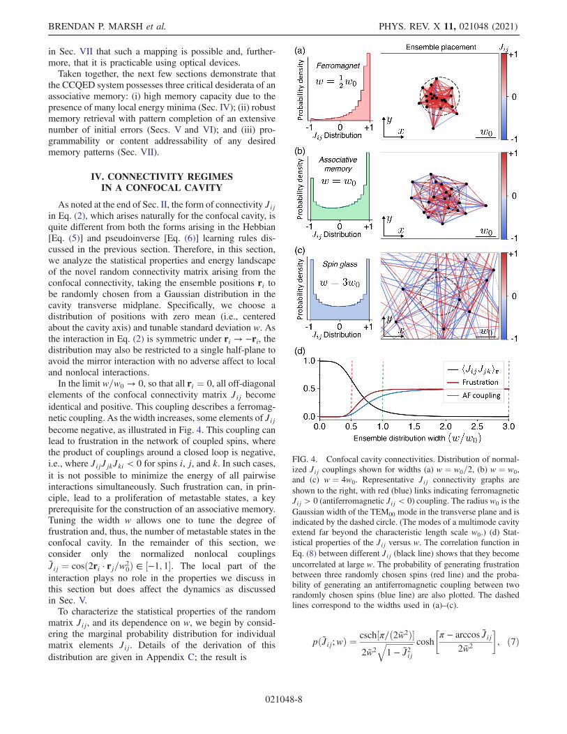
As noted at the end of Sec. II, the form of connectivity Jijin Eq. (2), which arises naturally for the confocal cavity, isquite different from both the forms arising in the Hebbian[Eq. (5)] and pseudoinverse [Eq. (6)] learning rules dis-cussed in the previous section. Therefore, in this section,we analyze the statistical properties and energy landscapeof the novel random connectivity matrix arising from theconfocal connectivity, taking the ensemble positions ri tobe randomly chosen from a Gaussian distribution in thecavity transverse midplane. Specifically, we choose adistribution of positions with zero mean (i.e., centeredabout the cavity axis) and tunable standard deviation w. Asthe interaction in Eq. (2) is symmetric under ri → −ri, thedistribution may also be restricted to a single half-plane toavoid the mirror interaction with no adverse affect to localand nonlocal interactions.In the limit w=w0 → 0, so that all ri ¼ 0, all off-diagonal

elements of the confocal connectivity matrix Jij becomeidentical and positive. This coupling describes a ferromag-netic coupling. As the width increases, some elements of Jijbecome negative, as illustrated in Fig. 4. This coupling canlead to frustration in the network of coupled spins, wherethe product of couplings around a closed loop is negative,i.e., where JijJjkJki < 0 for spins i, j, and k. In such cases,it is not possible to minimize the energy of all pairwiseinteractions simultaneously. Such frustration can, in prin-ciple, lead to a proliferation of metastable states, a keyprerequisite for the construction of an associative memory.Tuning the width w allows one to tune the degree offrustration and, thus, the number of metastable states in theconfocal cavity. In the remainder of this section, weconsider only the normalized nonlocal couplingsJij ¼ cosð2ri · rj=w2

0Þ ∈ ½−1; 1�. The local part of theinteraction plays no role in the properties we discuss inthis section but does affect the dynamics as discussedin Sec. V.To characterize the statistical properties of the random

matrix Jij, and its dependence on w, we begin by consid-ering the marginal probability distribution for individualmatrix elements Jij. Details of the derivation of thisdistribution are given in Appendix C; the result is

pðJij;wÞ ¼csch½π=ð2w2Þ�2w2

ffiffiffiffiffiffiffiffiffiffiffiffiffiffi1 − J2ij

q cosh

�π − arccos Jij

2w2

�; ð7Þ

FIG. 4. Confocal cavity connectivities. Distribution of normal-ized Jij couplings shown for widths (a) w ¼ w0=2, (b) w ¼ w0,and (c) w ¼ 4w0. Representative Jij connectivity graphs areshown to the right, with red (blue) links indicating ferromagneticJij > 0 (antiferromagnetic Jij < 0) coupling. The radius w0 is theGaussian width of the TEM00 mode in the transverse plane and isindicated by the dashed circle. (The modes of a multimode cavityextend far beyond the characteristic length scale w0.) (d) Stat-istical properties of the Jij versus w. The correlation function inEq. (8) between different Jij (black line) shows that they becomeuncorrelated at large w. The probability of generating frustrationbetween three randomly chosen spins (red line) and the proba-bility of generating an antiferromagnetic coupling between tworandomly chosen spins (blue line) are also plotted. The dashedlines correspond to the widths used in (a)–(c).


021048-8

where w≡ w=w0. Figures 4(a)–4(c) illustrate the evolutionof this marginal distribution for increasing width. For smallw, the distribution is tightly peaked around Jij ¼ þ1,corresponding to an unfrustrated all-to-all ferromagneticmodel, with only a single global minimum (up to Z2

symmetry). As w increases, negative (antiferromagnet)elements of Jij become increasingly probable. Also plottedin Fig. 4(d) are the fractions of Jij links that are anti-ferromagnetic as well as the fraction that realize frustratedtriples of spin connectivity, JijJjkJki < 0. The probabilityof antiferromagnetic coupling is analytically calculated inAppendix C, while the probability of frustrated triples isevaluated numerically.If the different matrix elements Jij were uncorrelated,

then one could anticipate that, as in the SK model,frustration would occur once the probability of negativeJij becomes sufficiently large. However, when correlationsexist, the presence of many negative elements is notsufficient to guarantee significant levels of frustrationand the consequent proliferation of metastable local energyminima. For example, the rank 1 connectivity Jij ¼ ξiξj,for a random vector ξ, can have an equal fraction of positiveand negative elements while remaining unfrustrated [68]. Ingeneral, we expect the couplings Jij and Jjk should becorrelated, as they both depend on the common position rj.As discussed in Appendix C, this correlation can becomputed analytically as a function of the width:

hJijJjkir ¼1

1þ 8w4; ð8Þ

where h·ir denotes an average over realizations of therandom placement of spin ensembles. Although correla-tions exist, we see from this expression that they decay like1=w4, so that, at large w, the correlations are weak; seeFig. 4(d). Of course, even weak correlations in a largenumber of OðN2Þ off-diagonal elements can, in principle,dramatically modify important emergent properties of therandom matrix, such as the induced multiplicity of meta-stable states and the statistical structure of the eigenvaluespectrum. Thus, we examine the properties of the actualcorrelated random matrix ensemble arising from the con-focal cavity rather than adopt known results.Figure 5 shows a numerical estimation of the number of

metastable states as a function of the width w. This numberis estimated by initializing a large number of random initialstates and allowing those states to relax via 0TMHdynamics until a metastable local energy minimum isfound. This routine is performed for many realizationsof the connectivity Jij and then averaged over realizationsto produce the number plotted in Fig. 5. We regardconfigurations which are related by an overall spin flipas equivalent. A single global minimum state exists at smallw with all spins aligned. This state defines the

ferromagnetic phase of the confocal connectivity. A phasetransition to an associative memory regime with multiplemetastable states occurs as w increases; this transitionbecomes increasingly sharp at larger system sizes. Finitesize scaling analysis of the transition yields a critical pointof wAM ≈ 0.67w0. Only the ferromagnetic global minimumexists below this value, while multiple minima emergeabove. The width wAM also marks the threshold at whichthe ferromagnetic state is no longer the global minimum ofthe energy. The number of metastable states, shown inFig. 5(b), increases rapidly for w > wAM. In particular, inthe range of w and N that we explore, we find that thefollowing fits the simulations:N ¼

ffiffiffiffiffiffiffiffiffiffiffiffiffiffiffiffiffiffi1þ AeBx

p, where x ¼

N1=νðw − wAMÞ=w0 is the rescaled width and A ¼ 0.33,B ¼ 3.4, and ν ¼ 2.4 are the fit parameters. Thus, thenumber of metastable states scales with N and w asOðewN0.4Þ just above wAM. At still larger w, the numericalestimation of this number becomes less reliable due to theincreasing prevalence of metastable states with small basinsof attraction under 0TMH dynamics [74].

FIG. 5. (a) Number of metastable states versus distributionwidthfor various system sizes N, as indicated. The average number ofmetastable states increases with N above the ferromagnetic-to-associative memory transition at wAM ¼ 0.67ð1Þw0. (b) Scalingcollapse of the above in the region 0.5w0 < w < 0.8w0, withdenser sampling. The x axis is rescaled as N1=νðw − wAMÞ=w0,while the y axis is unchanged. The parameters ν and wAM aredetermined by fitting the collapsed data to an exponential formffiffiffiffiffiffiffiffiffiffiffiffiffiffiffiffiffiffi1þ AeBx

p, where x ¼ N1=νðw − wAMÞ=w0. The uncertainties are

one standard error.


021048-9

The existence of multiple (metastable) local energyminima is a critical prerequisite for associative memorystorage. An additional requirement, as discussed in Sec. III,is that these local energy minima should possess largeenough basins of attraction to enable robust patterncompletion of partial or corrupted initial states, throughthe intrinsic dynamics of the CCQED system. As of yet, wehave made no statement about the basins of attraction of themetastable states we have found; we examine this issue inthe next two sections, which focus on the CCQEDdynamics. For now, we simply note that, at a fixed widthof w an Oð1Þ amount above the transition, the number ofmetastable states N grows with system size N as OðeN0.4Þ,while the total configuration space grows with exponentialscaling 2N . Given that every configuration must flow to oneof these energy minima, it seems reasonable to expect thatany energy-minimizing dynamics should endow theseminima with sufficiently large basins of attraction to enablerobust pattern completion, assuming these basins are allapproximately similar in size.At fixed N, the growth in the number of energy minima

as a function of w, depicted in Fig. 5, suggests thepossibility of a spin glass phase wherein exponentiallymany metastable local energy minima emerge. Based onthe analysis of the marginal Eq. (7) and pairwise Eq. (8)statistics of the matrix elements, we expect that the spinglass phase should be like that of an SK model at large w.To determine if such a state exists, we further analyze theconnectivity in this large w regime by comparing propertiesof the CCQED connectivity to those of the SK spin glassconnectivity. In the limit of large w, the probability densityfor the Jij given in Eq. (7) takes the limiting formpðJijÞ ¼ ð1 − J2ijÞ−1=2=π. This functional form differs fromthe SK spin glass model in which the probability density ofthe couplings is Gaussian, with only the first two momentsnonzero. However, it is known [75] that the SK model freeenergy depends on only the first two moments of themarginal distribution in the thermodynamic limit, as longas the third-order cumulant of the distribution is bounded.This fact is also true for the CCQED connectivity. Moreover,these first two moments in the CCQED connectivity can becomputed analytically. The mean μJ and standard deviationσJ as a function of width are, respectively,

μJ ¼1

1þ 4w4; σJ ¼

4w4

1þ 4w4

ffiffiffiffiffiffiffiffiffiffiffiffiffiffiffiffiffiffiffi5þ 8w4

1þ 16w4

s: ð9Þ

Thus, at large width, the mean is negligible compared to thestandard deviation, which is required for a spin glass (asopposed to ferromagnetic state).However, a key difference between the CCQED con-

nectivity and the SK connectivity is the presence ofcorrelations between different matrix elements. The form-er’s correlation strength decreases with width; see Eq. (8)

and Fig. 4(d). We can obtain insights into how large thewidth must be in order to suppress these correlations,thereby crossing into an SK-like spin glass phase, bycomparing the statistical structure of the CCQED connec-tivity eigenvalue distribution to that of the SK modelconnectivity. In particular, the eigenvalue distributionobeys the same Wigner’s semicircular law fWignerðxÞ ¼ffiffiffiffiffiffiffiffiffiffiffiffiffi4 − x2

p=2π as does the SK connectivity with zero mean

independent and identically distributed Gaussian elementsof variance 1=N [76,77]. Moreover, the distribution ofspacings s between adjacent eigenvalues (normalizedby the mean distance) in both obey Wigner’s surmisepWignerðsÞ ¼ ðπs=2Þe−πs2=4, reflecting repulsion betweenadjacent eigenvalues [78]. Figures 6(a) and 6(b) plot theeigenvalue distribution fwðxÞ and level-spacing distributionpwðsÞ for several widths w for the CCQED connectivity.Both distributions approach those of the SK model forwidths beyond a few w0. As we discuss next, the requiredratio w=w0 to reach the SK regime depends on the systemsize N.Figure 6(c) plots the difference between the confocal

eigenvalue distribution, denoted by fw, and the Wignersemicircular law fWigner in terms of the Hellinger distance,which is defined for arbitrary probability distributions pðxÞand qðxÞ as H2ðp; qÞ ¼ R dx½ ffiffiffiffiffiffiffiffiffiffi

pðxÞp−

ffiffiffiffiffiffiffiffiffiqðxÞp �2=2. The

distance metric equals 1 for completely nonoverlappingdistributions and 0 for identical distributions. We find thatthe Hellinger distance follows a universal (N-independent)curve as a function of wN−1=4. The structure of this curvedemonstrates that as long as w > wSK ¼ αN1=4w0, where αis a constant of the order of unity, then the spectrum of theconfocal cavity connectivity assumes Wigner’s semicircu-lar law, just like that of the SK model connectivity. At thislarge value of w, the strength of correlations betweendifferent matrix elements in the confocal cavity, given byEq. (8), isOð1=NÞ. Such weak correlations, combined withan Oð1Þ variance and a negligible mean of the matrixelements, endow the CCQED connectivity with similarspectral properties to that of the SK connectivity. Giventhese similarities, we thus expect that the CCQED modelpossesses an SK-like spin glass phase at widths w > wSK.While the Hellinger distance in Fig. 6(c) falls to zero, it

does so smoothly as N1=4. This result is suggestive of asmooth crossover between the associative memory andspin glass regimes; however, further investigation into spinglass order parameters and replica symmetry breaking iswarranted to clarify the nature of the transition. Moreover,at intermediate widths w < wSK, in which correlationsbetween the matrix elements of Jij arising from the spatialstructure of the cosð2ri · rj=w2

0Þ interaction are not sup-pressed as strongly as Oð1=NÞ, the low-lying energyconfigurations may exhibit interesting spatial structurecharacteristic of Euclidean disorder in other settings[79–81]. An analysis of this potential structure remainsfor future work.


021048-10

Figure 7 summarizes the three regimes of the CCQEDconnectivity matrix. The system is in a ferromagnetic phaseat small w=w0 with a phase transition to an associativememory regime at wAM ≈ 0.67w0. The associative memoryregime is marked by the proliferation of a large number ofmetastable states whose number scales as OðeN0.4Þ close towAM. These states possess large basins of attraction that aresuitable for associative memory. At still larger widths, theconnectivity closely resembles that of an SK spin glass.Further investigation is required to clarify whether thetransition between the associative memory and spin glassregime is sharp or simply a crossover. The evolution fromferromagnetic, to associative memory, to spin glass versusw is analogous to the behavior exhibited by the Hopfieldmodel as the ratio P=N of the number of memory patternsto neurons increases in the Hebbian connectivity. Havingdemonstrated that a significant number of metastable statesexist in the cavity QED system, Sec. V now discusses thenatural dynamics of the cavity. We show that these differfrom standard 0TMH or Glauber dynamics. As mentioned,changing the dynamics changes the basins of attractionassociated with each metastable state. Remarkably, as weshow in Sec. VI, the CCQED dynamics leads to a dramaticincrease in the robustness of the associative memory byensuring that many metastable states with sufficiently largebasins for robust pattern completion exist. These metastablestates persist even at large w, enabling recall of memories inboth the associative memory and spin glass regimes of theCCQED connectivity.

FIG. 6. Eigenvalue spectrum of the CCQED connectivity,demonstrating random matrix statistics. (a) The eigenvaluedistribution fw and (b) level-spacing spectrum for the nonlocalinteraction matrix Jij ¼ cosð2ri · rj=w2

0Þ. N ¼ 1000 spins areaveraged over 50 realizations of Jij matrices. The distributionsare shown for w ¼ 2w0 (red), w ¼ 3w0 (green), and w ¼ 12w0

(blue). Each distribution is normalized to have unit variance. Thesolid black lines show the Wigner semicircle eigenvalue distri-bution (a) and the Wigner surmise for the level-spacing distri-bution of Gaussian orthogonal ensemble random matrices (b).(c) shows the Hellinger distance between the averaged CCQEDconnectivity eigenvalue distribution fw [shown in (a)] and theWigner semicircle distribution fWigner. The distance is plotted as afunction of the rescaled width N1=νw=w0 for different power lawsν ¼ −3;−4;−5 corresponding to different colors, as indicated.Lines of varying intensity correspond to different N ranging fromN ¼ 100 (faintest) to N ¼ 1000 (darkest). The traces overlapwell for the ν ¼ −4 scaling.

FIG. 7. Regimes of CCQED connectivity behavior versuswidth w and system size N. The three shaded regions correspondto ferromagnetic (F), associative memory, and SK-like spin glass(SG) regimes, as discussed in the text. Note that associativememories can still be encoded even in the spin glass regime dueto SD dynamics; see Secs. V and VII.


021048-11

V. SPIN DYNAMICS OF THE SUPERRADIANTCAVITY QED SYSTEM

We now discuss the spin dynamics arising intrinsicallyfor atoms pumped within an optical cavity. To do so, westart from a full model of coupled photons and spins andshow how both the connectivity matrix discussed aboveand the natural dynamics emerge. Aspects of these arepresented in earlier work; e.g., the idea of deriving anassociative memory model from coupled spins and photonsis discussed in Refs. [24,25], with spin dynamics discussedin Ref. [32]. Because—as we discuss in Sec. VI—theprecise form of the open-system dynamics is crucial to thepossibility of memory recovery, we include a full discus-sion of those dynamics here to make this paper self-contained.Our discussion of the spin dynamics proceeds in several

steps. Here, we start from a model of atomic spins coupledto cavity photon modes; this model is derived inAppendix A. We then discuss how to adiabatically elimi-nate the cavity modes in the regime of strong pumping andin the presence of dephasing, leading to a master equationfor only the atomic spins. This equation describes rates ofprocesses in which a single atomic spin flips, and theserates include a superradiant enhancement, dependent on thestate of other spins in the same ensemble. Such dynamicscan be simulated stochastically. Finally, we show how, forlarge enough ensembles, a deterministic equation for theaverage magnetization of the ensemble can be derived. Thisequation is shown to describe a discrete form of steepestdescent dynamics.The system dynamics is given by the master equation

_ρ ¼ −i½H; ρ� þ κXm

L½am�; ð10Þ

wheream is the annihilation operator for themth cavitymodeand the Lindblad superoperator is L½X� ¼ 2XρX†−fX†X; ρg. The dissipative terms describe cavity loss at arate κ [82]. This process is the only dissipative process weconsider. Other processes, such as spontaneous emission,which could cause dephasing of individual spins are stronglysuppressed, because the pump laser frequency is sufficientlyfar detuned from the atomic excited state [56,60].Nevertheless,we address the effects of spontaneous emissionbelow.As derived in Appendix A, the Hamiltonian takes the

form of a multimode generalization of the Hepp-Lieb-Dicke model [60,83–85]:

H ¼Xm

½−Δma†mam þ φmða†m þ amÞ�

þ ωz

XNi¼1

Szi þXNi¼1

Xm

gimSxi ða†m þ amÞ þ χðtÞXNi¼1

Sxi :

ð11Þ

The first two terms describe the cavity alone. We work inthe rotating frame of the transverse pump: Δm denotes thedetuning of the transverse pump from themth cavity mode.We assume that the transverse pump is red detuned, and soΔm < 0. We also include a longitudinal pumping term,written in the transverse mode basis as φm. Such a pumpallows one to input memory patterns (possibly corrupted)into the cavity QED system.To describe the atomic ensembles, we introduce collec-

tive spin operators Sαi ¼ 1=2P

Mj¼1 σ

αj , where σαj are the

Pauli operators for the individual spins within the ithlocalized ensemble, which contains M spins. We assumeeach ensemble is sufficiently confined that we can approxi-mate all atoms in the ensemble as having the same spatialcoordinate and, thus, the same coupling to the cavity light.With this assumption, our model contains no terms thatchange the modulus of the spin in a given ensemble; i.e.,P

αðSαi Þ2 is conserved. As noted above, spontaneousemission terms, which can change this spin modulus, arestrongly suppressed. The term ωzS

zi describes the bare

level splitting between the atomic spin states. The coup-ling between photons and spins is denoted gim ¼ΞmðriÞΩg0 cosðϕmÞ=ΔA. This expression involves thetransverse profile ΞmðrÞ of the mth cavity mode and theeffect from the Gouy phase cosðϕmÞ; see Appendix A. For aconfocal cavity, these are Hermite-Gaussian modes; theirproperties are extensively discussed elsewhere [36,38,39,41].The final term in Eq. (11) introduces a classical noise

source χðtÞ. In Appendix D, we show this couplinggenerates dephasing in the Sx subspace so as to restrictthe dynamics to classical states, simplifying the dynamics.Such noise may arise naturally from noise in the Ramanlasers. In addition, such a term can also be deliberatelyenhanced either through increasing such noise or byintroducing a microwave noise source oscillating aroundωz. We choose to consider the dynamics with such a noiseterm to enable us to draw comparisons to other classicalassociative memories. We again assume this noise couplesequally to all atoms in a given ensemble. Without such aterm, understanding the spin-flip dynamics would be farmore complicated, as it would require a much larger statespace, with arbitrary quantum states of the spins. Exploringthis quantum dynamics, when this noise is suppressed, is atopic for future work, as we discuss in Sec. VIII.We note that spontaneous emission does lead to two effects

detrimental to the preservation of associative memory:motional heating and population escape from the computa-tional basis of atomic states. (A third effect, dephasing, onlysupplements the dephasing purposefully added to the schemeto suppress unwanted coherence.) The random momentumkicks from spontaneous emission eventually lead to theheating of atoms out of the trapping potential. Heating mightbe suppressible through, e.g., intermittent Raman-sidebandcooling [86] in the tightly confined optical trapping potentials.The shelving of population outside the j1;−1i and j2;−2i


021048-12

states can be repumped back into this computational basis bythe addition of two repumping lasers. That is, effectingresonant σ− transitions on the F¼F0 ¼ 1 and F¼F0 ¼ 2lines can halt magnetization decay. Thus, there exist effectivemitigation strategies to reduce the detrimental effects ofspontaneous emission.This multimode, multiensemble generalization of the

open Dicke model exhibits a normal-to-superradiant phasetransition, similar to that known for the single-mode Dickemodel. The effects of multiple cavity modes have beenconsidered for a smooth distribution of atoms [87,88], whereit is shown that beyond-mean-field physics can change thenature of the transition. In contrast, in Eq. (11), we considerensembles that are small compared to the length scaleassociated with the cavity field resolving power [89], soall atoms in an ensemble act identically. As such, in theabsence of interensemble coupling, the normal-to-super-radiant phase transition occurs independently for eachensemble of M atoms at the mean-field point gi;eff ¼ gc,where 4Mg2c ¼ ωzðΔ2

C þ κ2Þ=ΔC and gi;eff is the effectivecoupling for ensemble i to a cavity supermode (a super-position of modes coupled by the dielectric response of thelocalized atomic ensemble) [35]. The normal phase ischaracterized by hSxi ¼ 0 and a rate ∝ M of coherentscattering of pump photons into the cavity modes. In thesuperradiant phase, hSxi ≠ 0, and the atoms coherentlyscatter the pump field at an enhanced rate ∝ M2. Thisscattering is experimentally observable via a macroscopicemission of photons from the cavity and a Z2 symmetrybreaking reflected in thephaseof the light (0orπ) [34,40,90].In the absence of coupling, each ensemble independently

chooses how to break the Z2 symmetry, i.e., whether topoint up or down. Photon exchange among the ensemblescouples their relative spin orientation and modifies thethreshold. When all N ensembles are phase locked in thisway, the coherent photon scattering into the cavity in thesuperradiant phase becomes ∝ ðNMÞ2, in contrast to ∝ NMin the normal phase. Throughout this paper, our focus is onunderstanding the effects of photon exchange, when thesystem is pumped with sufficient strength that all theensembles are already deep into the superradiant regime.The behavior near threshold and shifts to the threshold dueto interensemble interactions are discussed again inSec. VIII. We now describe how to consider the collectivespin ensemble dynamics deep in the superradiant regime.To obtain an atom-only description deep in the super-

radiant regime, it is useful to displace the photon operatorsby their mean-field expectations for a given spin state:am → am þ ðφm þPi gimS

xi Þ=ðΔm þ iκÞ. This displace-

ment can be done via a Lang-Firsov polaron transformation[91,92], as defined by the unitary operator:

U ¼ exp

�XNi¼1

Xm

ðφm þ gimSxi Þ�

a†mΔm þ iκ

− H:c:

��: ð12Þ

Note that this transformation remains unitary even with theinclusion of cavity loss κ. The polaron transform changesboth the Hamiltonian and the Lindblad parts of the masterequation, redistributing terms between them. The trans-formed dissipation term remains κ

Pm L½am�, while the

transformed Hamiltonian is

H ¼ −Xm

Δma†mam þHHopfield

þ ωz

2

XNi¼1

ðiDF;iS−i þ H:c:Þ þ χðtÞXNi¼1

Sxi : ð13Þ

We define polaron displacement operators as

DF;i ¼ exp

�Xm

gim

�a†m

Δm þ iκ− H:c:

��; ð14Þ

and S�i ¼ Syi � iSzi are the (ensemble) raising and loweringoperators in the Sx basis. The Hopfield Hamiltonianemerges naturally from this transform:

HHopfield ¼ −XNi; j¼1


hiSxi ; ð15Þ

with the connectivity and longitudinal field given, respec-tively, by

Jij ¼ −Xm

ΔmgimgjmΔ2

m þ κ2; hi ¼ −2

Xm

φmΔmgimΔ2

m þ κ2: ð16Þ

With the Hamiltonian in the form of Eq. (13), we cannow adiabatically eliminate the cavity modes by treatingthe term proportional to ωz perturbatively via the Bloch-Redfield procedure. As derived in Appendix D, thisprocedure yields the atomic spin-only master equation

_ρ ¼ −i½Heff ; ρ� þXNi¼1

fKiðδϵþi ÞL½Sþi � þ Kiðδϵ−i ÞL½S−i �g:

ð17Þ

In the above expression, Heff ¼ HHopfield þHLamb is aneffective Hamiltonian including a Lamb shift contribution[93] that is written explicitly in Eq. (E19). Moreover,KiðδϵÞ is a rate function discussed below, and δϵþi (δϵ−i ) arethe changes in energy of HHopfield after increasing (decreas-ing) the x component of collective spin in the ith ensemble.Note that, although this expression involves ensemble-raising and -lowering operations, the master equationdescribes processes where the spin increases or decreasesby one unit at a time. For brevity, we refer to theseprocesses as spin flips below. Because these are collective


021048-13

spin operators, there is a “superradiant enhancement” ofthese rates, as we discuss below in Sec. V B.As mentioned above, classical noise dephases the quan-

tum state into the Sx subspace in which each ensembleexists in an Sxi eigenstate. By doing so, the state may bedescribed by the vector ðsx1; sx2;…; sx3Þ, where sxi is the Sxieigenvalue of the ith spin ensemble. Since Heff commuteswith Sx, it generates no dynamics in this subspace. Thedynamics thus arises solely through the dissipativeLindblad terms, corresponding to incoherent Sx spin-flipevents.The energy difference, upon changing the spin of the ith

ensemble by one unit �1, can be explicitly written as

δϵ�i ¼ −Jii ∓ 2XNj¼1

Jijsxj : ð18Þ

For the terms with j ≠ i, these represent the usual spin-flipenergy in a Hopfield model. An additional self-interactionterm Jiið∓ 2sxi þ 1Þ arises from the energy cost of chang-ing the overall spin of the ith ensemble. The self-interactionJii thus provides a cost for the ith spin to deviate fromsxi ¼ �Si, where Si ¼ M=2 is the modulus of spin ofensemble i. As written in Eq. (2), Jii is enhanced by a termβ, dependent on the size of the atomic ensembles. Ifsufficiently large, this enhancement could freeze all ensem-bles in place, by making any configuration with all sxi ¼�Si a local minimum. However, the strength of Jii can bereduced by tuning slightly away from confocality, whichsmears out the local interaction [36]. We see below that, forthe realistic parameters employed in Sec. II, no suchfreezing is observed. It is important to note that the largestself-interaction energy cost occurs at the first spin flip of agiven ensemble—i.e., subsequent spin flips become easier,not harder. One may also note that, as the size of ensembleM increases, the interaction strength ratio of the self-interaction to the interaction from other ensembles is notaffected; Eq. (18) shows all terms increase linearly withensemble size.As derived in Appendix D, the functions that then

determine the rates of spin transitions take the form

KiðδϵÞ ¼ω2z

8ReZ

∞

0

dτ exp

�−iδϵτ − CðτÞ

−Xm

g2imðΔ2

m þ κ2Þ ð1 − e−ðκ−iΔmÞτÞ�; ð19Þ

where the function CðτÞ depends on the correlations of theclassical noise source χðtÞ. It does so via JcðωÞ, the Fouriertransform of hχðtÞχð0Þi, using

CðτÞ ¼Z

∞

0

dω2π

JcðωÞω2

sin2�ωτ

2

�: ð20Þ

Details of the derivation of this expression are given inAppendix D, along with explicit calculations for an Ohmicnoise source.

A. Spin-flip rates in a far-detuned confocal cavity

We now show how the expressions for the spin-flip rateKðδϵÞ simplify for a degenerate, far-detuned confocalcavity. In an ideal confocal cavity, degenerate families ofmodes exist with all modes in a given family having thesame parity. Considering a pump near to resonance withone such family, we may restrict the mode summation tothat family and take Δm ¼ ΔC for all modesm. In this case,the sum over modes in Eq. (19) simplifies and becomesproportional to Jii. If we further assumeΔC ≫ Jii—the far-detuned regime—we can Taylor expand the exponential inEq. (19) to obtain the simpler spin-flip rate function

KiðδϵÞ ¼ hðδϵÞ þ e−Jii=jΔCjJiiω2zκ

8jΔCj½ðδϵ − ΔCÞ2 þ κ2� ; ð21Þ

where hðδϵÞ is a sharply peaked function centered onδϵ ¼ 0. Its precise form depends on the spectral density ofthe noise source and is given explicitly in Appendix D.Classical noise broadens hðδϵÞ into a finite-width peak.Considering experimentally realistic parameters, this widthis at least an order of magnitude narrower than the range oftypical spin-flip energies. As a result, its presence does notsignificantly affect the dynamics. The main contribution tothe spin-flip rate, thus, comes from the second term, aLorentzian centered at δϵ ¼ ΔC.Figure 8(a) plots the spin-flip rate of Eq. (21). By choosing

negative ΔC—i.e., red detuning—the negative offset of theLorentzian peak from δϵ ¼ 0 ensures that energy-loweringspin flips occur at a higher rate than energy-raising spin flips,thereby generating cooling dynamics. We can further definean effective temperature for the dynamics for spin-flipenergies sufficiently small in magnitude. To show this result,we inspect the ratio of energy-lowering to energy-raisingspin-flip ratesKðδϵÞ=Kð−δϵÞ. To obey detailed balance—asoccurs if coupling to a thermal bath—this ratiomust be of theformexpð−δϵ=TÞ, whereT is the temperature of the bath. Forsmall jδϵj, this constraint means one should compare the rateratio to a linear fit:

KiðδϵÞKið−δϵÞ

≈ 1 −δϵ

Teff; Teff ¼

Δ2C þ κ2

4jΔCj: ð22Þ

To determine whether this temperature is large or small, itshould be compared to a typical spin-flip energy δϵ: Thesystem is hot (cold) when the ratio Teff=δϵ is much greater(less) than unity. The ratio of spin-flip rates is shown inFig. 8(b), along with the Boltzmann factor using Teff definedinEq. (22). The rate ratio shows a small kink close to jδϵj ¼ 0arising from the noise term but otherwise closelymatches theexponential decay up until jδϵj ≃ jΔCj. We may ensure the


021048-14

spin-flip energies are ≤ jΔCj by choosing a pump strengthΩ ∝ ΔC=

ffiffiffiffiffiM

p. The spin dynamics drive the system toward a

thermal-like state in this regime.Despite the presence of an effective thermal bath, the

dynamics arising from the confocal cavity are ratherdifferent from those of the standard finite-temperatureGlauber or Metropolis-Hastings dynamics. This differencecan be seen by comparing the functions KðδϵÞ that wouldcorrespond to these dynamics. Glauber dynamics imple-ments a rate function of the form

KGlauberðδϵÞ ∝expð−δϵ=TÞ

1þ expð−δϵ=TÞ ; ð23Þ

while for Metropolis-Hastings

KMHðδϵÞ ∝�1 δϵ ≤ 0;

expð−δϵ=TÞ δϵ > 0:ð24Þ

The zero-temperature limits of both these functions are stepfunctions; e.g., K0TMH ∝ Θð−δϵÞ. These functions areplotted in Fig. 8(a), taking T ¼ Teff with an arbitraryoverall rescaling to match the low-energy rate of the cavityQED dynamics. The cavity QED dynamics exhibits anenhancement in the energy-lowering spin-flip rates peakedat ΔC. By contrast, the rate function for Metropolis-Hastings dynamics is constant for all energy-lowering spinflips. It is nearly constant at low temperatures for Glauberdynamics. In comparison, the cavity QED dynamicsspecifically favors those spin flips that dissipate moreenergy—the cavity allows these spins to flip at a higherrate. As we see in Sec. VI, this “greedy” approach to steadystate significantly changes the basins of attraction of thefixed points.Whether the cavity dynamics drive the spin ensembles to

a high-temperature or low-temperature state depends on theratio of the effective temperature and the typical energychange upon flipping a spin ensemble from one polarizedstate to the other. Employing a single atom per ensemblewith a small coupling strength leads to hot dynamics. Thisresult is because the pump strength Ω must be set such thatthe single spin-flip energy jδϵij < ΔC, which ensures thatthe spin-flip rate KðδϵÞ favors energy-lowering spin flipsover energy-raising ones, as shown in Fig. 8. This con-straint restricts Teff=jδϵij > 1=4, even though one wouldwant this ratio to be much less than unity to achieve a low-energy state.In contrast, low-temperature states may be reached by

employing many spins per ensemble. The superradiantenhancement ensures that all individual spins within anensemble align with each other, punctuated only by rapidevents during which the ensemble flips from one polari-zation to the other. The energy scale associated with thiscollective spin flip is δϵ�i ≡Mδϵi, given M atoms perensemble. The ratio of Teff=δϵ�i ∝ 1=M can then be madesmall by increasing M, effectively yielding a very lowtemperature. In the case of large M, therefore, the cavitydynamics is almost identical to that at zero temperature.The large values of M obtainable in our CCQED systemprovide access to the low-temperature regime. Moreover,we note that finite-temperature dynamics of the Hopfieldmodel have been thoroughly studied [16], and the model isknown to exhibit a robust recall phase even at a finitetemperature. As such, a lower-M regime would also exhibita similarly robust recall phase.The assumption that all ensembles are fully polarized is

well founded: As noted earlier, the on-site interactions Jiidrive the spins within an ensemble to align as if the systemwere composed of rigid (easy-axis) Ising spins. Moreover,the spin ensemble spin-flip rates are superradiantlyenhanced, meaning that the time duration of any ensembleflip is short and ∝ 1=M. As described below, the super-radiant enhancement also reduces the timescale required toreach equilibrium. As we discuss in Sec. VIII, to reach the

FIG. 8. (a) The spin-flip rate function KðδϵÞ in the confocallimit (solid line) versus spin-flip energy δϵ. Units are in terms ofthe pump-cavity detuning jΔCj. Rates for Metropolis-Hastings(dashed line) and Glauber (dotted line) dynamics are also shown.(b) Ratio of energy-decreasing to energy-increasing spin-fliprates Kð�δϵÞ versus spin-flip energy (solid line). Comparingfinite-temperature Metropolis Hastings dynamics (dashed line) tothe actual cavity dynamics allows one to identify a low-energyeffective temperature Teff ¼ ðΔ2

C þ κ2Þ=4jΔCj [59,60,95].


021048-15

quantum regime would require us to consider M ≃ 1,which, in turn, requires enhancements of the single-atomcooperativity so that the low-temperature regime may bereached at the level of single atoms per node.

B. Stochastic unraveling of the master equation

To directly simulate Eq. (17), we make use of a standardmethod for studying the time evolution of a masterequation: stochastic unraveling into quantum trajectories[96,97]. In this method, the unitary Hamiltonian dynamicsare punctuated by stochastic jumps due to the Lindbladoperators. For our time-local master equation, the dynamicsrealizes a Markov chain. That is, the evolution of the statedepends solely on the current spin configuration and thetransition probabilities described by the spin-flip rates.Moreover, the transition probabilities are the same for allspins within a given ensemble.A stochastic unraveling proceeds as follows. An initial

state is provided as a vector s ¼ ðsx1; sx2;…; sxNÞ. TheLindblad terms in the master equation (17) describe thetotal rates at which spin flips occur. However, the totalspin-flip rates additionally experience a superradiantenhancement from the matrix elements of S�i . The collec-tive spin-flip rates within an ensemble are, thus,

½SiðSi þ 1Þ − sxi ðsxi � 1Þ�Kiðδϵ�i Þ; ð25Þ

where the upper (lower) sign indicates the up (down) fliprate. As such, the rate of transitions within a givenensemble increases as that ensemble begins to flip, reachinga maximum when sxi ¼ 0, and then decreases as theensemble completes its orientation switch. The ensemblespin-flip rates are computed for each ensemble at everytime step. To determine which spin is flipped, waiting timesare sampled from an exponential distribution using thetotal spin-flip up and down rate for each ensemble. Theensemble with the shortest sampled waiting time is chosento undergo a single spin flip. The time in the simulationthen advances by the waiting time for that spin flip. Theprocess then repeats. This process requires the total rates tobe recomputed at every time step for the duration of thesimulation. Results of such an approach are shown inFig. 9(a).

C. Deterministic dynamics for large spin ensembles

A full microscopic description of the atomic spin statesbecomes unwieldy when considering large numbers ofatoms per ensemble. Fortunately, the large number of atomsalso means the full microscopic dynamics becomes unnec-essary for describing the experimentally observable quan-tities. The relevant quantity describing an ensemble is notthe multitude of microscopic spin states for each atom butthe net macroscopic spin state of the ensemble. We cantherefore build upon the above treatment to produce adeterministic macroscopic description of the dynamics:

Our approach is to construct a mean-field description that isindividually applied to each ensemble. This descriptionbecomes exact in the thermodynamic limit Si → ∞ andfaithfully captures the physics of ensembles with ≥103

atoms under realistic experimental parameters.We begin by defining the macroscopic variables we use

to describe the system. These are the normalized magne-tizations of the spin ensembles mi ≡ hSxi i=Si ∈ ½−1; 1� thatdepend on the constituent atoms via only their sum. Themiremain ofOð1Þ independent of Si, while fluctuations due to

FIG. 9. (a) Simulation of a system of N ¼ 100 ensembles. Allare initialized in a local minimum state except five ensembles thatare flipped in the wrong orientation. Each ensemble is composedof M ¼ 2S ¼ 105 spins. For this (realistic) number of spins, thestatistical fluctuations, which are present, are not resolvable.A comparison is made between dynamics derived from theequations of motion in the thermodynamic limit (dashed lines)and a full stochastic unraveling of the master equation (solidlines). The five traces show relaxation of those five spinensembles to the local minimum state. The other N − 3 spinensembles remain magnetized at �1 and are plotted in black.Data from the stochastic master equation simulation lie close tothat of the equation of motion. The timescale associated withspontaneous decay is marked by a dotted vertical line; the systemreaches steady state beforehand. Spontaneous emission caninduce motional heating and demagnetization of the ensemblesif mitigating actions are not taken, such as repumping andsideband cooling; see the text. All parameters are as listed inSec. II and ωz ¼ 1 MHz. (b) The total energy versus time, inunits of SjΔCj. As expected of discrete steepest descent dynam-ics, steps are clearly visible, and they occur in order of the energyremoved per spin flip.


021048-16

the random flipping of spins within the ensemble scale∝ 1=

ffiffiffiffiSi

p. The fluctuations about the mean-field value,

thus, become negligible at large Si, and the mi followdeterministic equations of motion. Following the derivationin Appendix F (see also Ref. [32]), we find that the mifollow the coupled differential equations

ddt

mi ¼ sgnðliÞSijKiðδϵþi Þ − Kiðδϵ−i Þjð1 −m2i Þ

þ Kiðδϵþi Þð1 −miÞ − Kiðδϵ−i Þð1þmiÞ; ð26Þ

where li ¼P

j JijSjmj is the local field experienced by theith ensemble, given the configuration of the other ensem-bles. The equations are coupled, because, as defined above,each δϵ�i ¼ −Jii ∓ 2

Pj JijSjmj. That is, the change of

the spin configuration energy as defined by HHopfield

[Eq. (15)] depends on all the other mj. Note that theself-interaction cost to flipping an atomic spin is largest forthe first spin that flips within a given ensemble.The term proportional to Si in Eq. (26) describes the

superradiant enhancement in the spin-flip rate. This termwould be zero if Si ¼ 1=2, since mi ¼ sxi =Si ¼ �1 in thatcase. For large ensembles, this term acts to rapidly align theensemble with the local field when jmij < 1. The otherterms act to provide the initial kick away from themagnetized jmij ¼ 1 states but receive no superradiantenhancement in the spin-flip rate. A separation of time-scales emerges between the rapid rate at which an ensembleflips itself to align with the local field, described by thesuperradiant term, and the slower rate at which an ensemblecan initiate a flip driven by the other terms. The dynamicsthat emerge correspond to periods of nearly constantmagnetizations jmij ¼ 1, punctuated by rapid ensemble-flipping events mi → −mi.To gain analytical insight into the equations of motion,

we make use of the separation of timescales that emerges inthe large Si limit. When the ensembles are not undergoinga spin-flip event, they are in nearly magnetized statesjmij ≈ 1 and can be approximated as constants. The spin-flip energies δϵ�i and rates KiðδϵÞ then become constant aswell. This result enables one to decouple the equations ofmotion Eq. (26) to consider the flip process of a singleensemble. This decoupling, in turn, provides a simpleanalytical solution for the time evolution of the flippingmagnetization:

miðtÞ¼ sgnðliÞ tanh ½SijKiðδϵþi Þ−Kiðδϵ−i Þjðt− ti0Þ�; ð27Þ

where the constants ti0 are determined from the initialconditions to be

ti0 ¼ −sgnðlimiÞ logð8SiÞ

8SijKiðδϵþi Þ − Kiðδϵ−i Þj: ð28Þ

These approximate solutions to the equations of motionaccurately predict that ensembles will flip to align withtheir local field, and the ordering of the ti0 predicts the orderin which the ensembles will flip. Ensembles that are alreadyaligned with the local field have a ti0 < 0 and will not flip inthe future unless the local field changes. On the other hand,ensembles not aligned with the local field have a ti0 > 0 andwill flip. The ensemble with the smallest ti0 > 0 will flipfirst. This result leads to a discrete version of steepestdescent dynamics, minimizing HHopfield from Eq. (15),since Eq. (28) implies that the smallest ti0 corresponds tothe largest energy change jδϵij. One may approximate allmi as constant up until the vicinity of the first ti0, at whichpoint the ith spin flips and alters the local fields. Theapproximation then holds again for the new local fieldsuntil the next spin-flip event occurs. This process continuesuntil convergence is achieved once all ensembles align withtheir local field. Overall, the mean-field dynamics takes asimple form: At every step, the system determines whichensemble would lower the energy the most by realigningitself and then realigns that ensemble in a collective spinflip, continuing until all δϵi > 0. The final configuration isa (meta)stable state corresponding to the minimum (or localminimum) of the energy landscape described by HHopfield.Figure 9(a) shows a typical instance of the dynamics

described by the equations of motion in Eqs. (26) andcompares it to a stochastic unraveling of the masterequation in Eq. (17). The 107 spins are divided into 100ensembles, each representing an S ¼ 105=2 collective spin.We use a Jij matrix constructed from the CCQED con-nectivity with spin distribution width w ¼ 1.5w0. Theensemble magnetizations are initialized close to a localminimum configuration. Specifically, five ensembles arechosen at random and misaligned with their local field,while the rest are aligned with their local field to specify theinitial condition. We see that the five initially misalignedensembles realign themselves to their local fields. Theirconvergence to the local minimum state described by theJij matrix occurs before the timescale set by spontaneousemission. We also see that the mean-field equations ofmotion closely match the stochastic unraveling.We confirm that these dynamics are consistent with SD

by considering the evolution of energy, as shown inFig. 9(b). The total energy of the spin ensembles mono-tonically decreases, with clearly visible steps correspond-ing to spin-flip events. These steps occur in order of largestdecrease in energy. The effect of SD dynamics on therobustness of stored memories, and, more generally, on thenature of basins of attraction in associative memorynetworks, remains unexplored to date. We address thisquestion in the next section.


021048-17

VI. IMPLICATIONS OF STEEPEST DECENTDYNAMICS FOR ASSOCIATIVE MEMORY

In the previous section, we find that, for large-spinensembles, the cavity-induced dynamics is of a discretesteepest descent form; i.e., at each time step, the next spin-flip event of an ensemble is that which lowers the energythe most. (This result is in contrast to 0TMH dynamics,where spins are flipped randomly provided that the spin fliplowers the energy.) We now explore how changing from0TMH to SD dynamics affects associative memories. Tounderstand the specific effects of the dynamics, in thissection, we consider both “standard” Hopfield neuralnetworks with connectivity matrices Jij drawn fromHebbian and pseudoinverse learning rules and SK spinglasses. We find that SD not only improves the robustnessand memory capacity of Hopfield networks, but also givesrise to extensive basins of attraction even in the spin glassregime. We note that the Hopfield model has a robustassociative memory phase even in the presence of a smallbut nonzero temperature [16]. Our results presented hereare not expected to change significantly when comparing tofinite-temperature Metropolis-Hastings dynamics or whenconsidering the effective temperature of the cavity dynam-ics for smaller spin ensembles. An introduction to Hopfieldneural networks is given in Sec. III.We compare 0TMH dynamics, where any spin flip that

lowers the energy of the current spin configuration isequally probable, versus SD dynamics, where the spin flipthat lowers the energy the most always occurs. Steepestdescent is a deterministic form of dynamics, while 0TMH isprobabilistic, and so fixed points can be expected to bemore robust under SD. We also note that natural SDdynamics, such as that exhibited by the pumped cavityQED system, is more efficient than simulated SD dynamics(given an equal effective time step duration). This result isbecause numerically checking all possible spin flips todetermine which provides the greatest descent is an OðN2Þoperation. Thus, interestingly, the natural steepest descentdynamics effectively yields an OðN2Þ speed-up oversimulations, by effectively computing a maximum oper-ation over N local fields (each of which is computed via asum over N spins) in Oð1Þ time.

A. Enhancing the robustness of classical associativememories through steepest descent

While the locations in configuration space of the localenergy minima of Eq. (4), or, equivalently, the fixed pointattractor states of Eq. (3), are entirely determined by theconnectivity Jij, the basins of attraction that flow to theseminima depend on the specific form of the energy-minimizing dynamics. To quantify the size of these basins,we require a measure of distance between states. A naturaldistance measure is the Hamming distance, defined asfollows. Consider two spin states s and s0 corresponding to

N-dimensional binary vectors with elements si ¼ �1. TheHamming distance between s and s0 is defined asd ¼PN

i¼1 jsi − s0ij=2. Thus, the Hamming distancebetween an attractor memory state and another initial statesimply counts the number of spin-flip errors in the initialstate relative to the attractor. This notion of Hammingdistance enables us to determine a memory recall curve forany given attractor state under any particular energy-minimizing dynamics. We first pick a random initial stateat a given Hamming distance d from the attractor state, byrandomly flipping d spins. We then check whether it flowsback to the original attractor state under the given dynami-cal scheme. If so, a successful pattern completion, ormemory recall event, has occurred. We compute theprobability of recall by computing the fraction of timeswe recover the original attractor state over random choicesof d spin flips from the initial state. This computation yieldsa memory recall probability curve as a function of d. Wedefine the size of the basin of attraction under the dynamicsto be the maximal d at which this recall curve remainsabove 0.95.Figure 10(a) shows memory recall curves, basin sizes,

and their dependence on the form of the energy-minimizingdynamics for a Hopfield network trained using the pseu-doinverse learning rule; see Eq. (6). Three different formsof dynamics are shown: 0TMH, SD, and the CCQEDdynamics of Eq. (26). As expected, the CCQED dynamicsclosely match the SD dynamics. The basin size depends ondynamics: SD and CCQED dynamics lead to a larger basinof attraction than 0TMH. Indeed, the entire memory recallcurve is higher for SD than 0TMH.This increase in the robustness of the memory, at least for

small d, leads directly to an increase in basin size. Tounderstand this result, consider the following argument.Imagine the Hamming surface of 2ðNdÞ configurations adistance d from a fixed point at the center of the surface.The recall curve pðdÞ is the probability the dynamicsreturns to the fixed point at the center of the surface whenstarting from a random point on the surface. Under 0TMH,due to the stochasticity of the random choice of spin flipthat lowers the energy, many individual configurations onthe Hamming ball could flow to multiple different fixedpoints, thereby lowering the probability pðdÞ for returningto the specific fixed point at the center of the Hammingsurface. However, under the deterministic SD dynamics,each point on the Hamming surface must flow to one andonly one fixed point. Of course, many points on theHamming surface could, in principle, flow under SD toa different fixed point other than the fixed point at thecenter. But, as verified in simulations (not shown), for smallenough d, more points on the Hamming surface flow underSD to the central fixed point than under 0TMH. As such,recall probability increases for small d, as indeed shown inFig. 10(a). This deterministic capture of many of the stateson the Hamming surface by the central fixed pointeffectively enhances the robustness of the memory.


021048-18

We can study how the SD and 0TMH dynamics affect thedependence of basin size on the number of patterns storedand, hence, the memory capacity. We separately considerthe two traditional learning rules, Hebbian and pseudoin-verse. In both cases, we expect a trade-off between thenumber of patterns P stored and the basin size, with thelatter shrinking as the former increases. Figures 10(b) and10(c) demonstrate this trade-off for both learning rules.However, in both cases, switching from 0TMH to SDameliorates this trade-off; at any level of memory load, theaverage basin size increases under SD versus 0TMH.To calculate each point, we generate P random desired

memory patterns ξμ in order to construct the Jij matrixaccording to the learning rule under consideration. For eachpattern, we determine its associated attractor state sμ. In thecase of the pseudoinverse learning rule, the attractor stateassociated with a desired memory ξμ is simply identical tothe desired memory. However, in the Hebbian rule, theassociated attractor state sμ is merely close to the desiredmemory ξμ. We find this attractor state sμ by initializing thenetwork at the desired memory ξμ and flowing to the firstfixed point under 0TMH. The inset in Fig. 10(b) plots theoverlap N−1P

i ξμi s

μi as a function of the pattern loading

α ¼ P=N of the Hebbian model. This overlap is close to 1for α < αc ≈ 0.138 and drops beyond that, indicating that,beyond capacity, the Hebbian rule cannot program fixedpoints close to the desired memories.We focus specifically on the fixed points sμ to dissociate

the issue of programming the locations of fixed points sμ

close to the desired memories ξμ from those of examiningthe basin size of existing fixed points and the dependence ofthis basin size on the dynamics. To determine the basin sizefor these fixed points, we compute the maximal input errorfor which the recall probability remains above 95%. Thiscomputation is performed for both learning rules underboth 0TMH and SD dynamics. We then average therecovered basin size over the P patterns.Figure 10(b) presents the results for Hebbian learning,

and SD dynamics appears to increase the basin size forpattern-loading ratios P=N > 0.1. Note that the basin sizeunder 0TMH is not extensive in the system size N beyondthe capacity limit P=N ¼ αc ≈ 0.138N. However, remark-ably, under SD the basin size of the fixed points sμ isextensive in N, despite the fact that the Hopfield model is ina spin glass phase at this point. Thus, the SD dynamics candramatically enlarge basin sizes compared to 0TMH, evenin a glassy phase. However, this enlargement of basin sizedoes not by itself constitute a solution to the problem oflimited associative memory capacity, because it does notaddress the programmability issue; above capacity, thefixed points sμ are not close to the desired memories ξμ; seeFig. 10(b), inset. Steepest descent can only enlarge basins,not change their locations. As such, for Hebbian learning,

FIG. 10. (a) Recall probability as a function of the inputerror applied, quantified by the Hamming distance between theinput and pattern state. This probability is plotted for threeforms of dynamics: 0TMH (red), SD (blue), and CCQED(orange). The latter is given by Eq. (26). This plot illustrateshow the dynamics affects recall probability and, thus, basin size(defined by the point where the recall curve drops below 95%).We use a connectivity matrix Jij corresponding to a pseudoin-verse Hopfield model with N ¼ 100 spins and P ¼ 0.6Npatterns stored. We choose this learning rule because itillustrates a large difference between the two dynamics.(b) Average basin size of attractors for connectivity of a Hebbianlearning rule. The intensity of the trace increases with systemsize, N ¼ 200, 400, 800, while color indicates the form ofdynamics. The critical ratio αc ≈ 0.138marks the known patternloading threshold where Hebbian learning fails in the thermo-dynamic limit [16]. Inset: overlap between the attractor of thedynamics sμ and the bare memory ξμ, as discussed in the text.(c) Average basin size for the pseudoinverse learning rule versusthe ratio of patterns stored to number of nodes, P=N. Steepestdescent dynamics outperforms 0TMH in all cases, yieldinglarger basin sizes for P=N ≳ 0.1 and, thus, greater memorycapacity.


021048-19

the memory capacity C ≈ 0.138N cannot be enhancedunder any choice of energy-minimizing dynamics unlessan additional programming step is implemented.In contrast to Hebbian learning, the pseudoinverse

learning rule does not have a programmability problemby construction. The connectivity possesses a fixed point sμ

identical to each desired memory ξμ. Figure 10(c) showsthat SD confers a significant increase in basin size forpseudoinverse learning as well. At large P=N, the basinsizes under SD are more than twice as large as under 0TMHdynamics.

B. Endowing conventional spin glasseswith associative-memory-like properties

Basin sizes do not typically scale extensively with Nunder 0TMH dynamics, because the number of metastablestates grows exponentially (in the system size N) in boththe Hopfield model (with Hebbian connectivity forP=N ≫ 0.138) and in the SK spin glass model [98].However, we now present numerical evidence that SDdynamics endows these same energy minima with basinsizes that exhibit extensive scaling with N, even in a pureSK spin glass model. Thus, we find that the SK spin glass,under the SD dynamics, behaves like an associativememory with an exponentially large number of memorystates with extensive basins. (A programming step isrequired; see Sec. VII B.)More quantitatively, we numerically compute the size of

basins present in an SK spin glass using both kinds ofdynamics; see Fig. 11. Connectivity matrices Jij areinitialized with each element drawn, independent andidentically distributed, as Gaussian random variables ofmean zero and variance 1; normalization of the variance isarbitrary at zero temperature. Rather than compute auniform average over all metastable states of the Jijmatrix—a task that is numerically intractable for largesystem sizes—we instead sample metastable states byinitializing random initial states and letting those statesevolve under 0TMH dynamics. Once a metastable state isreached, the basin of attraction is measured under both0TMH and SD dynamics as discussed above.Figure 11(a) plots the average basin size as a function of

the system size N, averaging both over realizations of Jijmatrices and over the random initial states. Under 0TMHdynamics, the mean basin size decreases with increasingN,approaching zero at large N. This result shows that, for0TMH dynamics, metastable states of the spin glassbecome very fragile, as expected from a traditional under-standing of metastable states in a spin glass. In contrast, forSD dynamics, the average basin size scales extensivelywith system size in a roughly linear fashion. A phenom-enological fit results in scaling of 0.0135ð1ÞN þ 0.91ð7Þ.These results help reveal the structure of the energy

landscape. Vanishing basin size under 0TMH implies that asingle spin-flip perturbation is sufficient to open new

pathways of energy descent to different local minima.As soon as such pathways exist, 0TMH will find them,leading to vanishing basin size. For SD, we, however, seethat the steepest path of energy descent is almost always theone leading back to the original local minimum that isperturbed, as long as the number of spin flips is less thanabout 0.0135N. This picture explains how metastable statesare stable against small perturbations under SD but unstableunder 0TMH.The extensive scaling of basin sizes found for SD

dynamics not only means that metastable states with afinite basin of attraction exist, but, in fact, suggests thenumber of such states is exponential in system size, fargreater than the capacity of any typical associative memory.While sampling metastable states via relaxation of randominitial states under the standard 0TMH dynamics does notyield a uniform sampling, Fig. 11(b) shows that nearly allsuch discovered metastable states have a finite basin ofattraction under SD dynamics. The distribution is peakedaway from zero basin size, whereas with 0TMH thedistribution is strongly peaked around zero. This resultsuggests that extensive basin sizes under SD dynamics may

FIG. 11. (a) Average basin size of randomly found localminima for the SK model using 0TMH (red) or SD (blue).The shaded region corresponds to �1 standard deviation in thebasin sizes. For each N, the basin size is averaged over 50realizations of Jij matrices, with 500 random initial states per Jijrealization. (b) Histogram of basin sizes using 0TMH (red) andSD (blue) for the N ¼ 1000 data plotted in (a). The mean basinsize for SD is marked by the vertical dashed line.


021048-20

be a property of almost all metastable states in the SKspin glass.We conclude that the SK spin glass enhanced with

SD dynamics operates, remarkably, like an associativememory, with exponentially many spurious memories.These memories are random and nonprogrammable viaany existing learning rule but have extensive basins ofattraction, tolerating up to 0.0135N input errors on averagewhile maintaining a 95% probability of recall. While thisbasin size is small compared to that of stored patterns instandard associative memories—cf. Fig. 10—it is never-theless extensive, and there are exponentially more suchmemories than in standard Hopfield networks.

VII. ASSOCIATIVE MEMORY IN PUMPEDCONFOCAL CAVITIES

We show in Sec. IV that CCQED supports a largenumber of metastable states and in Sec. V that the naturalcavity QED dynamics produces a discrete SD dynamics inenergy. In Sec. VI, we show that SD dynamics can enhancethe robustness of memory when applied to traditionalHopfield models and, moreover, can endow the SK spinglass with associative-memory-like properties.In this section, we pull these key elements together to

demonstrate how robust associative memory can be createdin a transversely pumped confocal cavity. We begin byshowing that metastable states in such systems indeedpossess large basins of attraction. We then develop amethod to solve the addressing or programmability prob-lem, which involves converting the patterns we wish tostore into the patterns that naturally arise as local energyminima with large basins of attraction. Our pattern storagescheme is applicable to any connectivity matrix Jij. Weverify its performance for the CCQED connectivity matrixboth in the associative memory regime and in the SK spinglass regime.

A. Basins of attraction with confocal cavityQED connectivity

We now examine the basin size of the metastable statesfound in Sec. IV by tuning the width w of the distribution ofensemble positions. We measure the basin size of meta-stable states just as we did in Fig. 10 for Hopfield modelsand Fig. 11 for the SK model—by the relaxation of randomperturbations. In particular, a random CCQED connectivitymatrix J is realized by sampling the spin ensemblepositions from a 2D Gaussian distribution of fixed widthw. A large number of random initial states are then preparedand allowed to relax via the native SD dynamics to ametastable state. The basin size of that metastable state isthen found by initializing nearby random states andestimating the probability that these perturbed states evolveback to the metastable state as a function of the Hammingdistance of the perturbation.

Figure 12 shows how the basin size evolves with w forthe CCQED connectivity. For each width w, the measuredbasin sizes are averaged over many realizations of theCCQED matrices J, with 200 random initial states permatrix. The number of realizations of J required forconvergence varies with N, ranging from 1600 realizationsfor N ¼ 3 spins to 32 realizations for N ¼ 800 spins. Thisvariation is due to self-averaging at large system size.Figure 12(a) presents the average basin size as a function ofw, using both the native SD dynamics and 0TMH forcomparison. A sharp decrease in basin size occurs near theferromagnetic-to-associative memory transition atwAM ≈ 0.67w0. For 0TMH dynamics, the mean basin sizeper spin quickly falls to zero after crossing wAM.Remarkably, however, steepest descent dynamics yieldslarger basins beyond wAM. These are extensive in size.Thus, just as in the case of the Hopfield model beyondcapacity and in the SK spin glass, switching from0TMH to SD dramatically expands the size of basinsfrom nonextensive to extensive. Moreover, there exist

FIG. 12. (a) The average basin size in the CCQED systemversus width of the spin ensemble distribution w. Metastablestates are found by relaxing random initial seeds. Basin sizes forboth 0TMH dynamics (red) and the (native) SD dynamics (blue)are shown. System sizes ranging from N ¼ 3 to N ¼ 800 areconsidered, with darker traces corresponding to larger sizes. Weextrapolate to the limit N → ∞ by fitting a linear function of1=N to the finite N data. The intercept at 1=N ¼ 0 yields thethermodynamic limit (dashed lines). The ferromagnetic-to-associative memory phase transition, indicating the onset ofmultiple metastable states, is marked by a vertical black dashedline at wAM. The green line shows the typical basin size under SDdynamics for the SK connectivity, 0.0135ð1ÞN, as extractedfrom Fig. 11. (b) Histogram of the basin sizes found for widthsw ¼ 1.5w0 and w ¼ 4w0.


021048-21

OðeN0.4Þ metastable states in this regime, which is less thanthe OðeNÞ expected of a spin glass; see Fig. 5. Overall, thisresult demonstrates that a confocal cavity in this inter-mediate width regime functions as a high-capacity, robustassociative memory with many metastable states withextensive basin sizes, albeit with random nonprogram-mable memories. For larger widths, the average basin sizeasymptotically reduces to that exhibited in the SK model.This observation, when combined with the analysis ofSec. IV, provides further evidence that the confocal cavityconnectivity yields an SK spin glass at large width.Figure 12(b) shows examples of the distribution of basin

sizes under SD dynamics for widths 1.5w0 and 4w0. Forw ¼ 1.5w0, the variance in basin sizes is large despite asmall mean size of approximately 0.05N. Pattern comple-tion is robust in this regime for a large percentage of basins,since many exceed 0.1N in size. For w ¼ 4w0, the basinsize distribution is narrower but still peaked away fromzero. However, nearly all basins sizes are less than 0.1N, asexpected in the spin glass regime; see Fig. 4(c).

B. Solving the programmability problem:A scheme for memory storage

We demonstrate in the previous subsection the presenceof many metastable states with large basins of attraction (ofextensive size) in the transversely pumped CCQED system.Such a system evidently manifests a robust recall phasewith a large number of random memories. However, thesememories are not directly programmable, in the sense thatwe cannot place the local energy minima wherever we wishin configuration space by tuning the connectivity. Thislimitation is in contrast to both the Hopfield model withHebbian connectivity, in which one can place up to 0.138Nenergy minima corresponding to ξμ in configuration spaceas long as these points are random and uncorrelated, and thepseudoinverse rule, which enables one to place localenergy minima at N arbitrary points. However, neitherschemes are readily realizable in physical systems withnatural dynamics.To store memories in the CCQED system, one might first

consider a simple method by which desired patterns areassociated with the local energy minimum that they flow tounder steepest descent dynamics. A slightly corruptedpattern state could then flow to the same local minimumand also be associated with the pattern. However, theprobability that nearby states flow to the same localminimum is high only when those states are themselvesnear to that local minimum. Numerical steepest descentsimulations show that random pattern states typically arenot near enough to any local energy minimum for thisprocess to occur, even in a glassy energy landscape. Assuch, this simple approach is not reliable, and an encodingstep that maps patterns to local energy minima is requiredso that the memories can enjoy the basin of attractionprovided by the local energy minima.

We now show how to effectively program the CCQEDsystem using an encoder. The scheme stores any desiredpattern using an encoder that assumes the form of a single-layer neural network. This network translates the desiredpatterns to be stored into the nonprogrammable metastablestates that are naturally stabilized by the intrinsic cavitydynamics. This translation is important, because the desiredpatterns, in general, have no correlation with the basins ofattraction naturally present in the cavity and cannot makeuse of those basins for pattern completion. The encodingscheme involves a linear transformation to the input patternfollowed by thresholding to ensure binary outputs. Thepattern storage scheme we present here is designed with thephysics of CCQED in mind and may be implemented in afully optical setting with spatial light modulators to imple-ment linear transformations of light fields [100]. Moreover,the thresholding is naturally provided by the cavity-spinsystem, because steepest descent dynamics drive the spinsinto a state of saturated magnetization. We describe thedetails of the experimental implementation below. Themethod is also applicable to any Hopfield or spin-glass-likenetwork connectivity with nonprogrammable energyminima possessing extensive basin sizes. We note thatthe problem of finding a mapping between two sets ofbinary states using a single-layer neural network is wellknown [101,102] and can be solved using a variety ofperceptron training methods. However, we find that thegreater nonlinearity of these maps causes the basins ofattraction realized by these schemes to become effectivelysmaller than those of the simpler scheme we present. Wechoose to not employ those methods.The basic idea behind the encoder is to find a linear

transformation that maps any set of desired patterns, asrepresented by light fields, into metastable spin configu-rations of the cavity. Once found, this transformation isthen applied to any input state (i.e., light field) beforeallowing the confocal cavity network to dynamicallyevolve to a metastable state. The (optical) output can thenundergo an inverse transform, back into the original basis.In this way, we harness the dynamics of the CCQED spinnetwork to store general patterns and recall them throughpattern completion, without ever needing to change theCCQED connectivity matrix.To formally define the properties required of the trans-

formation M, we consider a set of patterns that we wish tostore, fΞpg for p ¼ 1 to P. We require that there are at leastPmetastable states of the Hopfield energy landscape fΦpgthat need to be found and cataloged. These may be foundby, e.g., allowing random initial states to relax—note thatthere may be more than P such states. For an arbitrary inputstate x, the network operates as follows.(1) The input state x is transformed to an encoded state

x ¼ MðxÞ. The transformation should smoothlymap the desired pattern states onto metastable statesof the Hopfield network: We thus require MðΞpÞ ¼Φp for all p.


021048-22

(2) The Hopfield network is initialized in the encodedstate x and allowed to evolve to a metastablestate y.

(3) The evolved state y is then subject to an inversetransformation M−1. The final output is y ¼M−1ðyÞ. The transformation M−1 should map themetastable states of the energy landscape back ontothe pattern states so that M−1ðΦpÞ ¼ Ξp. Note thatM−1½MðΞpÞ� ¼ Ξp, so that M and M−1 act asinverse transformations when acting on pattern states.

We now discuss how to find the smooth transformationsM and M−1 obeying the properties above. The simplestoption is a linear transformation, for which we shoulddefine MðxÞ ¼ M · x, where M is the matrix that mini-mizes the error function

E ¼XPp¼1

jM · Ξp − Φpj2 þ λjjMjj2: ð29Þ

Here, jj · jj is the Hilbert-Schmidt norm. The terms in thesum ensure that the patterns are mapped to the metastablestates of the cavity QED system. However, this requirementunderconstrainsM for P < N. To remedy this shortcoming,we add the term λjjMjj2 to penalize large elements of M;λ is a regularization hyperparameter. This least-squaresproblem can be solved analytically, yielding

M ¼�XP

p¼1

ΦpΞpT

��λ1þ

XPp¼1

ΞpΞpT

�−1: ð30Þ

In addition, a thresholding operation is required to ensureeach binary input state is encoded to another binary state.Spin configurations x should correspond to vectors whoseelements are�1, corresponding to the magnetization of theSx components of the spin ensembles. Thus, we modify theencoding so that the full transformation for an arbitraryinput state is MðxÞ ¼ sgnðM · xÞ, where the sign functionis understood to be applied elementwise. This transforma-tion plays the role of the threshold operation when viewingthe encoding scheme as a neural network.The encoder matrix defined in Eq. (30) is not invertible,

in general. However, by simply reversing the roles of thepatterns and cavity minima in constructing the encodermatrix, we can construct a corresponding decoder matrixthat maps the metastable states back to the desired patterns:

M−1 ¼�XP

p¼1

ΞpΦpT

��λ1þ

XPp¼1

ΦpΦpT

�−1: ð31Þ

The memory capacity of an associative memory istypically defined as the maximum number of patterns thatcan be stored as metastable states of the energy landscape.Under this standard definition, at most N total patterns can

be mapped exactly onto attractor states of the CCQEDconnectivity, because the transformation map is linear. Thisconstraint means that the maximummemory capacity of theencoded confocal cavity is N, which is the same as that ofthe pseudoinverse learning method but significantly out-performs Hebbian learning with its capacity of approx-imately 0.138N. However, a more practical definition ofcapacity would depend also on the size of the basins ofattraction and, hence, the robustness of the stored patterns.We now verify the memory capacity of N accounting forbasin size.We numerically benchmark the encoded pattern storage

methodwith the CCQED connectivity and SDdynamics thatare present in the cavity. Fixing the system size N, wegenerateP randompatterns to store in the cavity. Because theCCQED connectivity hosts a large number of metastablestateswith large basins in the regimewAM ≤ w ≤ 2w0, we setthe width w to 1.5w0 to construct a connectivity matrix.Metastable states are cataloged by relaxing P random initialseeds using SD. (Note that this procedure is biased towardselecting metastable states with the largest basins of attrac-tion; these are preferable for our scheme.) This procedure isthen followed by construction of the encoder and decoderusing Eqs. (30) and (31). The basin sizes of the pattern statesare determined by applying increasing amounts of inputerror to the patterns until the probability of recall dropsbelow 95%.Figure 13 compares the performance of encoding

memories onto the metastable states of the CCQEDconnectivity against the results of Hebbian and pseudoin-verse learning. The average basin size of our CCQEDscheme is larger than Hebbian learning. The results do not

FIG. 13. Average basin size of patterns stored in a CCQEDsystem as a function of P=N using the linear transformationencoding scheme (yellow line). Results are shown for N ¼ 800;however, similar results are found for system sizes ofN ¼ 50–800.For comparison, the average basin sizes are plotted for theHebbian(red line) and pseudoinverse (blue line) learning methods. In eachcase, we show the results of both SD (more intense lines) and0TMH (less intense lines) dynamics; w ¼ 1.5w0.


021048-23

depend strongly on system size. For the CCQED scheme,extensive basin sizes are indeed observed up to themaximum P ¼ N stored patterns. This memory capacityrepresents roughly an order-of-magnitude improvementover the standard Hebbian learning model (0.138N) andcoincides with the pseudoinverse learning rule. The basinsizes in CCQED are not as large as pseudoinverse learning,though they are more physically realizable. Note that, forthe Hebbian learning, we measure recall as the probabilityof recovering the desired memory. As such, the drift oflocal minima from the desired patterns contributes to thecollapse of basin size at P=N ¼ 0.138.Remarkably, we find that, for memory loading ratios

P=N ≤ 0.4, the average basin size with the encoding anddecoding transformation significantly exceeds 0.1N. Thisresult is notable, because earlier we found that the averagebasin sizes are less than 0.1N at this width, w ¼ 1.5w0; seeFig. 12. It seems that the encoding and decoding trans-formations significantly enhance the robustness of theassociative memory. Inspection of the form of the lineartransformation reveals that it focuses the P < N input statesonto a subset of the metastable states and vice versa for thedecoder matrix. This focus effectively gives it a head startby reducing the Hamming distance between perturbedinput states and the nearest metastable state.The pattern storage scheme also works in the SK spin

glass regime, as applied either to the CCQED connectivityat large w or to the actual SK model. In both cases, Nmemories may be stored. The linear transformation schemeis thus quite flexible: It is applicable to any model withextensively scaling basins of attraction. An interestingchallenge for future work would be to see if it is possibleto extend the current scheme to nonlinear mappingsbetween pattern states and attractors in order to achievea superextensive scaling of the memory capacity withsystem size N. This scaling would provide a physicallyrealizable fully programmable associative memory withcapacity well beyond the P ¼ N pattern limit. In this case,the fact that the SK spin glass possesses an exponentialnumber of metastable states with extensive basin sizesunder SD dynamics could become particularly relevant forassociative memory applications.

C.Weight chaos and the robustness of memory patterns

Considering the practical implementation of the asso-ciative memory, an important question is that of “weightchaos” [103–106]. More specifically, for standard Hopfieldlearning rules, flipping the sign of a few (or even one) Jijmatrix elements can result in a model with a completelydifferent set of metastable states. This problem arisesdue to the chaotic nature of glassy systems. In our case,weight chaos can arise from two sources. Imprecisionin the placement of spin ensembles leads to fluctuationsin the positions ri and, thus, in the nonlocal inter-action Jij ∼ cosð2ri · rj=w2

0Þ. Additionally, atom number

fluctuations per spin ensemble can occur between exper-imental realizations, leading to fluctuations in Jij propor-tional to 1=

ffiffiffiffiffiM

p. Neither of these can change the sign of

large Jij elements, thereby avoiding the most severe,randomizing repercussions of weight chaos.The effect of weight chaos is numerically explored in

Fig. 14 under experimentally realistic parameters. Weconsider an uncertainty of 1 μm in the placement of spinensembles and fix the total number of atoms in the cavity atP

Ni¼1M ¼ 106 independent of the number of ensembles

considered. We then present two different measures ofweight chaos and its effect, as a function of the ensembledistribution width w. First, we quantify how metastablestates drift between realizations. To do so, we take aparticular Jmatrix and find a metastable state s by allowinga random initial state to relax via SD. We then realize aweight matrix J0 that is nominally the same as J but hasadded to it a particular realization of position and atomnumber noise. The state s is then allowed to again relax viaSD to a potentially new state s0 to see if it has drifted.The overlap s · s0=N quantifies this drift and is shown inFig. 14(a) for many realizations. In the second measure, wedirectly quantify the change in the weights as a percentage

FIG. 14. The effect of weight chaos in experimental parameterregimes, using an ensemble placement uncertainty of 1 μm and1=

ffiffiffiffiffiM

pfluctuations in atom number. The drift of metastable states

between different realizations of noise weights is plotted in (a) asa function of the width w of the ensemble distribution and fordifferent system sizes N [see the legend in (b)]. The states s and s0refer to metastable states of two realizations J and J0, respectively,as described in the text. (b) The direct change in the Jconnectivity matrix is plotted as a function of the width.


021048-24

of their original values via the quantity kJ − J0k=kJk,where k · k denotes the Hilbert-Schmidt norm of the matrix.Figure 14 demonstrates that metastable states are robust

against drift for widths less than approximately w0, whichincludes the ferromagnetic and associative memoryregimes of the confocal connectivity. Greater than 98%overlap between experimental realizations is expected. Theoverlap begins to drop for widths beyond w0 as theconnectivity transitions to a spin glass, because the non-local connectivity becomes increasingly sensitive to posi-tion at larger radii. The overlap decreases with increasingsystem sizes in this regime up to the maximum N ¼ 400ensembles probed in simulations. Atom number fluctua-tions set a floor on weight chaos that is independent of w.This floor is visible in Fig. 14(b) for small w. The noisefloor rises with increasing N, since M must decrease inorder to fix the total atom number. A few percent deviationin Jij is acceptable for heuristic solvers, replacing one“good-enough” solution with another. Position uncertaintyis likely smaller than 1 μm, so these results present aconservative picture.

D. Experimental implementation

We now present practical details of how the CCQEDassociative memory can be initialized in a particular (dis-torted) memory state. One may initialize the spin ensemblesvia longitudinal pumping to an arbitrary (encoded) x, wherexi ¼ �1 is the magnetization of the ith ensemble. As seen inEq. (15), the spins can be subjected to a field hi created bylongitudinally pumping the cavity. Physically, this pumpingscheme is possible because in a confocal cavity, resonantlight with any transverse profile (up to the resolvingcapability of the cavity mirrors) is supported due to thedegeneracy of all TEMlm modes of good parity. If thelongitudinal pumping is sufficiently strong, i.e., φi > Jij,then the energy of spin flips δϵi is dominated by this field. Bychoosing sgnðφiÞ ¼ xi, SDdynamics evolve the spin ensem-bles into statex. The fact that only thepatternof signsmattersfor large fields presents a natural implementation of thethreshold operation employed in the encoding MðxÞ. Thelongitudinal pump is turned off once the state is initialized,thereby allowing the system to evolve to the nearby meta-stable state determined by the connectivity Jij alone.Many schemes would suffice for implementing the

encoding and decoding transformations mentioned above.The transformation can be accomplished most simplyelectronically. In this scheme, a new longitudinal field isoptically constructed based on the electronically trans-formed state. Similarly, after imaging the cavity light, thedecoder matrix is applied electronically to yield the finaloutput state from the experiment. Alternatively, an all-optical implementation can be achieved using spatial lightmodulators or other methods [100] if coherence in the fieldmust be preserved.

VIII. DISCUSSION

We presented a practicable quantum-optical system thatcan serve as a neural network for associativememory. It doesso by exploiting the natural spin coupling and superradiantdynamics provided by a CCQED system. The physicalsystem lacks the direct correspondence between memoriesand the connectivitymatrix thatmakes simple the learning ofpatterns in the idealized Hopfield model. Nevertheless, wefind a straightforward pattern storage scheme for encod-ing memories in this physical system that allows N memo-ries to be stored with a robust pattern-completion processthat tolerates an extensive number of initial errors.Remarkably, the emergent SD dynamics of the physicalsystem extend the effective basins of attraction to enablerobust recall. In terms of memory capacity, the systemsignificantly outperforms Hebbian learning.The multimode cavity QED platform is distinctive among

annealing-based optimization schemes for its nonequili-brium dynamics. In “traditional” annealing approaches,the system undergoes either classical equilibrium dynamicsin a potential landscape [107] or unitary quantum dynamicsremaining close to the ground state [108]. In the CCQEDsystem, the optimization occurs by the intrinsic dynamics ofa driven-dissipative system. By contrast, in equilibriumcontexts, any coupling to the outside world disrupts thesystem: Dissipation must be overcome in these approaches,not embraced as in the present scheme.Confocal cavity QED can be compared to other gain-

based optimization schemes. These include weak-coupling,optics-based “coherent Ising machines.” These explore thenotion that optimization problems can be heuristicallysolved using the dissipative coupling between multipleoptical parametric oscillators (OPOs) [48,49,109,110]. Thesteady-state pattern of the oscillator phases that develops atthreshold manifests the solution to this problem. Thissolution occurs because the coupling of OPOs is chosenso that the pattern of oscillation with lowest thresholdcorresponds to the solution of the optimization problem. Assuch, as one increases the pumping, this lowest thresholdsolution appears first. Similar ideas have also been exploredin coupled polariton condensates [50] and lasers [111].There are, however, crucial limitations to these weakly

coupled optical gain-based optimizers: The output spinstates correspond to coherent photon states, which emergeonly as one crosses the threshold. This limitation meansthat, near threshold, the spins are “soft,” allowing defects toform [112]. In addition, because the photon number is notconserved, photon intensity in each node can change,leading to dynamic changes in the Jij weights definingthe problem [113]. This limitation requires the addition ofclassical feedback to control these populations [114–116].By contrast, the multimode cavity QED system has anearly constant number of atoms per ensemble, so theconnectivity matrix Jij remains stable. The spin variablesare well defined far above the superradiant threshold: The


021048-25

superradiant enhancement of the dynamics forces ensem-bles to flip as one collective spin. We also point out that,while the fully quantum limit of the CCQED systemconsists of a single strongly coupled atom at each positionand so the state space becomes that of spin 1=2 particles, incontrast, the photonic or polaritonic coherent Isingmachines possess (continuous) bosonic Hilbert spaces.An important challenge for future work is to extend the

present treatment into the fully quantum realm. Thisextension could be done by suppressing the dephasingwe use to favor classical states, tuning pump strength nearto the superradiant phase transition, and considering fewspins per ensemble. As noted earlier, currently we require alarge number of atoms per ensemble to overcome heating;an alternative would be to design a configuration withenhanced single-atom cooperativity. While the cooperativ-ity of a single 87Rb atom coupled to TEM00 mode is C ¼2g20=κΓ ¼ 5.2 in our system [34,40], the system shouldadditionally benefit from an enhanced cooperativity for anatom coupled to many degenerate modes with nonzero fieldamplitude at its location. That is, the single-atom cooper-ativity is enhanced by the number of degenerate modes, dueto the formation of a “supermode” with a larger electricfield at the atom’s position [35,36]. The confocal cooper-ativity is, therefore, far greater than unity; preliminarymeasurements suggest it is approximately 50 [36]. Ifachieved, this cooperativity would allow quantum entan-glement to play a role in the dynamics [118], enabling theexploration of the behavior of a fully quantum nonequili-brium neural network. Whether and how entanglement andquantum critical dynamics at the superradiant phase tran-sition provide superior heuristic solution-finding capabilityremains unclear. When the number of cavity modes is muchsmaller than the number of atoms, exact solutions areknown in both thermal equilibrium [28] and dissipativesystems [33]. Such exact solutions, however, rely on asemiclassical limit becoming valid for large numbers ofatoms, which is a regime where quantum effects thereforevanish. Specific questions of interest include how entan-glement might affect memory capacity or retrieval fidelity.We leave these questions for future exploration. Beyondquantum neuromorphic computing, such systems might beable to address quantum many-body problems [119].Finally, we note that our pattern storage and recall

scheme provides a novel shift in paradigm from thetraditional Hopfield framework of memory storage.Indeed, in this traditional framework, desired memories,as determined by network states driven by external stimuli(i.e., the patterns ξμ in Sec. III), are assumed to be directlystabilized by a particular choice of connectivity matrix J.For example, the Hebbian rule [Eq. (5)] and the pseudoin-verse rule [Eq. (6)] are two traditional prescriptions fortranslating desired memories ξμ into connection patterns Jthat engineer energy minima at or near the desiredmemories. In contrast, the steepest descent dynamics in

our system reveals that random choices of connectivity J,whether originating from the CCQED system, a glassyHopfield model beyond capacity, or remarkably, even thecanonical SK spin glass, yield Ising systems possessingexponentially many local energy minima with extensivebasin size. Indeed, our storage scheme exploits this intrinsi-cally occurring multiplicity of robust minima simply bymapping external stimuli ξμ to them rather than creatingnew minima close to the external stimuli. To date, thiscomputational exploitation of the exponential multiplicityof local energy minima in glassy systems has not beenpossible because of their subextensive basin size undertraditional 0TMH or Glauber dynamics. By contrast, theintrinsic physical dynamics we discover in the CCQEDsystem directly enables us to computationally harness theexponential multistability of glassy phases, by using anencoder to translate external stimuli to natively occurringinternally generated patterns. Further exploitation of theseglassy states through nonlinear encoders remains anintriguing direction for future work.Interestingly, in biological neural systems, multiple brain

regions, like the hippocampus and the cerebellum, that arethought to implement associative memories, are synapti-cally downstream of other brain regions that are thought torecode sensory representations before memory storage; see,e.g., Ref. [120] for a review. Such brain regions could playthe role of an encoder that learns to translate sensory stimuliinto natively occurring memory patterns, in analogy to ourstorage framework. Moreover, there is some neurobiolog-ical evidence that natively occurring neural activity patternsobserved before an experience are themselves used toencode that new experience [121,122], though there isdebate about the prevalence of this observation [123]. Ofcourse, if neurobiological memory encoding does indeedselect one of a large number of latent, preexisting stableactivity patterns in order to encode a novel stimulus, it maybe very difficult to experimentally observe such a stableactivity pattern before presentation of the stimulus, due tolimited availability of recording time. Thus, our worksuggests it may be worth explorations beyond theHopfield framework for memory storage, in which theinternal representations of memories are determined notonly by the nature of sensory stimuli themselves, but alsoby the very nature of natively occurring potential stablememory states that exist, but are not necessarily expressed,before the onset of the stimulus.Thus, overall, by combining the biological principles of

neural computation with the intrinsic physical dynamics ofa CCQED system, our work leads to enhanced associativememories with higher capacity and robustness, opens up anovel design space for exploring the computational capa-bilities of quantum-optical neural networks, and empowersthe exploration of a novel paradigm for memory storageand recall, with implications for how we might bothcomputationally harness the energy landscapes of glassy


021048-26

systems as well as explore novel theoretical frameworks forthe neurobiological underpinnings of memory formation.

The research data supporting this publication can beaccessed at [124].

ACKNOWLEDGMENTS

We thank Daniel Fisher and Hideo Mabuchi for stimu-lating conversations and acknowledge the Army ResearchOffice for funding support. The authors thank NTTResearch for their financial support. We also thank theStanford Research Computing Center for providing com-putational resources, especially access to the Sherlockcluster. Y. G. and B. P. M. acknowledge funding from theStanford Q-FARM Graduate Student Fellowship and theNational Science Foundation (NSF) Graduate ResearchFellowship, respectively. J. K. acknowledges support fromthe Leverhulme Trust (IAF-2014-025), and Surya Ganguliacknowledges funding from the James S. McDonnell andSimons Foundations and an NSF Career Award.

APPENDIX A: RAMAN COUPLING SCHEMEAND EFFECTIVE HAMILTONIAN

The effective multimode Dicke model in Eq. (11) may beengineered by coupling two internal states of 87Rb to the cavityfields as proposed in Ref. [56]; see Fig. 2. The scheme isdemonstrated in the dispersive limit (yielding an effective Isingmodel) using a cavity capable of multimode (confocal)operation [37]. The states jF¼2;mF¼−2i≡j↑i andjF ¼ 1; mF ¼ −1i≡ j↓i are coupled through two cavity-assisted two-photon Raman processes depicted in Fig. 2. Thetwo states j↑i and j↓i are separated in energy by ωHF due tohyperfine splitting and Zeeman shifts in the presence of atransversely oriented magnetic field. Typical experimentsemploy a magnetic field of approximately 2.8 G. The hyper-fine level splitting is ωHF ≈ 6.8 GHz. The cavity resonancefrequency ωC is detuned from the atomic excited state 52P3=2

by Δþ and Δ−, respectively, for states j↑i and j↓i. Twostanding-wave transverse pump beams with Rabi frequenciesΩ� realize the two cavity-assisted Raman processes. Theoptical frequencies of the pump beams ω� are given by

1

2ðωþ − ω−Þ ¼ ωHF − ωz;

1

2ðωþ þ ω−Þ ¼ ωC þ ΔC; ðA1Þ

where ωz is the two-photon Raman detuning and ΔC is thedetuning of the mean frequency of the pumps from the cavityresonance.To derive the model in Eq. (11), we extend the results

and experimental setup in Ref. [37] to the present case of amultimode cavity of confocal configuration. The fieldprofile of a single transverse mode with mode index m ¼ðl;mÞ in a cavity of length L is given by

Φm ¼ ΞmðrÞ cos�k

�zþ r2

2RðzÞ�− θmðzÞ

�; ðA2Þ

where ΞmðrÞ are the Hermite-Gauss mode functions and

θmðzÞ ¼ ψðzÞ þ nm½ψðL=2Þ þ ψðzÞ� − ξ; ðA3Þ

ψðzÞ ¼ arctan

�zzR

�; ðA4Þ

RðzÞ ¼ zþ z2Rz: ðA5Þ

Here, ξ is a phase offset fixed by the boundary conditionthat the light field vanishes at the two mirrors z ¼ L=2,nm ≡ lþm is the sum of the two transverse indices, k ¼2π=λ780 is the wave vector of the pump and cavity light, andzR ¼ L=2 is the Rayleigh range of a confocal cavity. Underthe Raman coupling scheme, the light-matter interactionHamiltonian for a multimode cavity can be obtained bysumming up the contributions from the transverse modes.In the appropriate rotating frame [37], the total HamiltonianH ¼ H↑ þH↓ þHcavity þHRaman is given by

H↑ ¼Z

d3xψ†↑ðxÞ

�p2

2mþ V trapðxÞ þ ωz

�ψ↑ðxÞ;

H↓ ¼Z

d3xψ†↓ðxÞ

�p2

2mþ V trapðxÞ

�ψ↓ðxÞ;

Hcavity ¼ −Xm

Δma†mam;

HRaman ¼Xm

Zd3x½η−mðxÞψ†

↑ðxÞψ↓ðxÞa†m

þ ηþmðxÞψ†↓ðxÞψ↑ðxÞa†m þ H:c:�; ðA6Þ

where ψ†↑;↓ are the spinor wave functions for the atomic

states, V trap is the trapping potential, and the cavity-assistedRaman coupling strength has spatial dependence given bythe cavity mode profile Φm and the standing-wave pumpalong the x direction:

η�mðxÞ ¼ffiffiffi3

pg0Ω�

12Δ�Φmðr; zÞ cosðkxÞ: ðA7Þ

The two Raman processes can be balanced by controllingthe pump beam power such that

ffiffiffi3

pg0Ωþ

12Δþ¼

ffiffiffi3

pg0Ω−

12Δ−≡ η: ðA8Þ

To remove the kinetic energy dependence and the spatialoscillation of the Raman coupling strength, we propose thefollowing trapping scheme for V trapðxÞ: First, introduce


021048-27

optical tweezers to tightly confine atoms in separate ensem-bles in different locations ri in the cavity transverse planebut at the midpoint of the cavity axis z ¼ 0; then, super-impose on the optical tweezers a deep 2D optical latticewith a periodicity of 780 nm along both the pump andcavity direction to add a potential V lattice ∝ cos2ðkx=2Þþcos2ðkz=2Þ. Under the combined trapping potential, thespinor wave function can be expanded as a sum of individualensembles

ψ↑↓ðxÞ ¼Xi;νi

ZðzÞffiffiffiffiffiffiffiffiffiffiffiffiffiffiffiffiffiffiρðr − riÞ

p×

ffiffiffiffiffiffiffiffiffiffiffiffiffiffiffiffiffiffiffiffiffiffiffiffiffiffiffiffiffiffiffiffiffiffiffiffiffiffiffiffiffiffiffiffiffiffiffiffiffiffiffi½1þ cosðkxÞ�½1þ cosðkzÞ�

pψ↑↓;νi ; ðA9Þ

where ZðzÞ and ρðrÞ describe the spatial confinement of anensemble by the optical tweezers trap, νi indexes individualspins inside an ensemble indexedwith i, and ψ↑↓;νi is the spinoperator for a single atom νi.For each ensemble with M atoms, we define collective

spin operators

Szi ¼XMνi¼1

ðψ†↑;νi

ψ↑;νi − ψ†↓;νi

ψ↓;νiÞ=2;

Sxi ¼XMνi¼1

ðψ†↑;νi

ψ↓;νi þ ψ†↓;νi

ψ↑;νiÞ=2: ðA10Þ

Taking the assumption that the width σA of the atom profileZðzÞ and ρðrÞ satisfies the condition λ780 ≪ σA ≪ zR, wecan perform the spatial integral along z and drop theoscillatory terms along x. The Raman coupling termbecomes

HRaman ¼Xm

XNi¼1

gimSxi ða†m þ amÞ; ðA11Þ

where the coupling strength between the ith ensemble andmth cavity mode gim is given by

gim ¼ η

2

Zd2rΞmðrÞρðr − riÞ cosðnmπ=4Þ ðA12Þ

and we assume that different ensembles are separated inspace with negligible overlap.Putting this together, the CCQED system can be

modeled by a master equation:

∂tρ ¼ −i½HCCQED; ρ� þXm

κL½amρ�: ðA13Þ

Here, we account for cavity field loss at rate κ by Lindbladsuperoperators L½X� ¼ XρX† − fX†X; ρg=2, where am isthe annihilation operator for the mth cavity mode. TheHamiltonian of the CCQED system HCCQED is given by

HCCQED ¼Xm

½−Δma†mam þφmða†m þ amÞ�

þωz

XNi¼1

Szi þXNi¼1

Xm

gimSxi ða†m þ amÞ: ðA14Þ

We always choose the transverse pump to be red detunedfrom the cavity modes so that Δm < 0. The mode-spacerepresentation of a longitudinal pump term is φm.We discuss the effects of additional classical and quantum

noise terms in the Hamiltonian in Appendixes D and E.

APPENDIX B: DERIVATION OF THECONFOCAL CONNECTIVITY

We now derive the form of the confocal connectivitypresented in Eq. (2). The starting point is the interactionbetween spin ensembles Eq. (16) that arises from thepolaron transformation presented in Sec. V. We considerthe limit of a confocal cavity, in which all even (or odd)Hermite-Gauss modes become degenerate so thatΔm ¼ ΔCfor all modes of the same parity. In this limit, the interactionin an even confocal cavity takes the form

Jij ¼−g20ΔC

Δ2C þ κ2

Xevenm

ΞmðriÞΞmðrjÞO2m; ðB1Þ

where ΞmðrÞ is the Hermite-Gauss mode function and thesum is taken over modes with indicesm ¼ ðl;mÞ for whichnm ≡ lþm is even. The term Om describes the overlap ofthe atoms with the longitudinal part of the cavity modes andis given by cosðnmπ=4Þ for even confocal cavities with spinensembles located at the cavity midplane [36]. The sumover of Hermite-Gauss mode functions is calculated usingthe known Green’s function of the harmonic oscillatorderived from the Mehler kernel:

Gðri; rj;φÞ ¼Xm

ΞmðriÞΞmðrjÞe−nmφ

¼ 1

πð1 − e−2φÞ exp�

2ri · rjw20 sinhðφÞ

−r2i þ r2j

w20 tanhðφÞ

�;

ðB2Þ

where φ ∈ C and the sum is taken over all Hermite-Gaussmodes. We make use of symmetry to restrict the sum toeven modes, noting that Ξmð−rÞ ¼ ð−1ÞnmΞmðrÞ. Thus, bysymmetrizing the above Green’s function, we may cancelthe odd terms while leaving the even terms. The Green’sfunction for an even confocal cavity is then given byGþðri; rj;φÞ ¼ ½Gðri; rj;φÞ þGðri;−rj;φÞ�=2. The inter-action (B1) is similar to the Green’s function but includesthe phase factors O2

m. These can be expanded in terms ofexponential functions to write the confocal interaction as


021048-28

Jij ¼−g20ΔC

2ðΔ2C þ κ2Þ ½G

þðri; rj; 0Þ þ Gþðri; rj; iπ=2Þ�: ðB3Þ

Evaluating the symmetrized Green’s functions yields

Jij ¼−g20ΔC

2ðΔ2C þ κ2Þ

�1

2δ

�ri − rjw0

�þ 1

2δ

�ri þ rjw0

�

þ 1

πcos

�2ri · rjw20

��: ðB4Þ

The delta functions represent local and mirror imageinteractions arising from the complete basis provided bythe Hermite-Gauss modes. The mirror image interaction∝ δ½ðri þ rjÞ=w0� may be avoided by placing all atomicensembles in the same half-plane of the cavity; we drop thisterm going forward. The nonlocal cosine interaction arisesdue to Gouy phase shifts of the Hermite-Gauss modes andprovides the connectivity between spin ensembles consid-ered throughout the paper.We now consider the effect of finite spatial extent of the

spin ensembles on the form of the interaction Jij. Theeffective interaction between ensembles is given by theconvolution of the interaction (B4) with the atomic ensem-ble density profiles ρiðxÞ:

Jij ¼−g20ΔC

2ðΔ2C þ κ2Þ

ZdxdyρiðxÞρjðyÞ

×�1

2δ

�x − yw0

�þ 1

πcos�2x · yw20

��: ðB5Þ

The ensemble densities may be approximated by Gaussianprofiles centered at positions ri of width σA. Performing theintegrals results in the effective interaction

Jij ¼−g20ΔC

2πðΔ2C þ κ2Þ

×

�βδij þ

expð−2σ2Aðjrij2þjrjj2Þw40þ4σ4A

Þ1þ 4σ4A=w

40

cos

�2w20ri · rj

w40 þ 4σ4A

��;

where β ¼ w20=ð8σ2AÞ is as presented in the text. The local

term ∝ β represents the strength of the local interactionwithin a spin ensemble and drives the superradiantenhancement of the spin dynamics. Above, we assumethat the distance between any two ensembles is muchgreater than σA so that different ensembles interact via onlythe nonlocal interaction. The effect of finite σA for thenonlocal interaction is to rescale the term inside the cosineand reduce its amplitude for ensembles located far from thecavity center. While a nonzero σA is necessary for the localinteraction to remain finite, the effect on the nonlocalinteraction is minimal for typical experiments in which

σA=w0 ≪ 1. We, therefore, take the limit σA=w0 ¼ 0 for thenonlocal term in the Jij interaction (2) presented in the text.

APPENDIX C: DERIVATION OFCONFOCAL CAVITY QED CONNECTIVITY

PROBABILITY DISTRIBUTION

Wenowderive the probability distribution and correlationsof the Jij matrices for the CCQED system with a Gaussiandistribution of atomic positions. We recall that the photon-mediated interaction takes the form Jij ∝ cosð2ri · rj=w2

0Þ,where w0 is the width of the TEM00 mode. We consider spinensemble positions ri to be randomlydistributed according toa 2D isotropic Gaussian distribution, centered at the origin ofthe cavity transverse plane and with a standard deviation w.Explicitly, ri ¼ ðri;x; ri;yÞT , where ri;k is a Gaussian randomvariablewithmean 0 and variancew2. To find the probabilitydistribution of Jij, we proceed by first finding the probabilitydistribution for ri · rj ¼ ri;xrj;x þ ri;yrj;y, the dot product of2DGaussian random variables. We start by writing the termsin the dot product as

ri;xrj;x ¼�ri;x þ rj;x

2

�2

−�ri;x − rj;x

2

�2

: ðC1Þ

The variances of ri;x and rj;x are equal, and their sum anddifference are independent random variables, each withvariance 2w2. This result implies that

ri;xrj;x ∼�N ð0; 2w2Þ

2

�2

−�N ð0; 2w2Þ

2

�2

∼w2

2½N ð0; 1Þ2 −N ð0; 1Þ2�; ðC2Þ

where∼ indicates equality in distribution and eachN ðμ; σ2Þdenotes an independentGaussian randomvariablewithmeanμ and variance σ2. Thus, the full dot product ri · rj isdistributed as

ri · rj ∼w2

2½N ð0; 1Þ2 −N ð0; 1Þ2 þN ð0; 1Þ2 −N ð0; 1Þ2�

∼w2

2½χ22 − χ22�; ðC3Þ

where χ2ν is a chi-square random variable with ν degrees offreedom. Themoment-generating function for this differenceof χ22 distributions is given by

Mχ22−χ2

2ðtÞ ¼ Mχ2

2ðtÞMχ2

2ð−tÞ ¼ 1=4

1=4 − t2: ðC4Þ

This moment-generating function corresponds to a knownprobability density for ri · rj which we denote pri·rjðxÞ;specifically,


021048-29

pri·rjðxÞ ¼1

2w2exp

�−jxjw2

�: ðC5Þ

We now wish to find the probability density pcosðxÞ forthe cosine of the random variable 2ri · rj=w2

0. Applying thegeneral formula [125] for taking functions of randomvariables allows us to write

pcosðxÞ ¼Xk;�

pri·rj

�w20

2cos−1k;�ðxÞ

�� ddxw20

2cos−1k ðxÞ

��; ðC6Þ

where by cos−1k;�ðxÞ we denote the infinite number ofpossible inverses of cosine; more precisely,

cos−1k;�ðxÞ ¼ � arccosðxÞ þ 2πk; k ∈ Z; ðC7Þ

where arccosðxÞ ∈ ½0; π� is the principal inverse of cosine.The derivative of cos−1k;�ðxÞ with respect to x appearingabove is independent of k:

ddx

cos−1k;�ðxÞ ¼∓ 1ffiffiffiffiffiffiffiffiffiffiffiffiffi1 − x2

p : ðC8Þ

Substituting in the derivative, we find

pcosðxÞ¼w20

2w2ffiffiffiffiffiffiffiffiffiffiffi1−x2

pX∞k¼−∞

exp

�−

w20

2w2jarccosðxÞþ2πkj

�:

ðC9Þ

Using the fact that j arccosðxÞj ≤ π, the infinite sum can berearranged as a geometric series:

pcosðxÞ ¼w20

2w2ffiffiffiffiffiffiffiffiffiffiffiffi1− x2

p�exp

�−w20 arccosðxÞ

2w2

�

þ 2 cosh

�w20 arccosðxÞ

2w2

�X∞k¼1

e−πkw20=w2

�: ðC10Þ

Evaluating the geometric series and rewriting in terms ofhyperbolic functions finally results in

pcosðxÞ ¼w20cschðπw

20

2w2Þ2w2

ffiffiffiffiffiffiffiffiffiffiffiffiffi1 − x2

p cosh

�w20

2w2ðπ − arccos xÞ

�: ðC11Þ

This probability density is the main result of this Appendix.We now present a number of quantities related to the

distribution of couplings. First, the mean of the probabilitydistribution can be computed in the usual way:

μJ ¼Z

1

−1xpcosðxÞdx ¼ 1

1þ 4ð ww0Þ4 ; ðC12Þ

as well as the variance

σ2J ¼Z

1

−1dxðx − μJÞ2pcosðxÞ

¼16ð ww0

Þ8½5þ 8ð ww0Þ4�

½1þ 4ð ww0Þ4�2½1þ 16ð ww0

Þ4� : ðC13Þ

We may also find the correlation between couplings as afunction of w. This correlation is important, for instance, incomparing the connectivity to that of an SK spin glass inwhich the couplings are uncorrelated. We first use atrigonometric identity to write

JijJjk¼ cos

�2ri ·rjw20

�cos

�2rj ·rkw20

�

¼1

2

�cos

�2

w20

rj ·ðriþrkÞ�þcos

�2

w20

rj ·ðri−rkÞ��

:

ðC14Þ

Since ri and rk are both Gaussian random variables withequal variances, their sum and difference are uncorrelatedGaussian random variables with twice the original variance.Thus, the two terms have the same expected value, and wefind

hJijJjki ¼cos

�2

w20

rj · ðri þ rkÞ�

¼cos

�2

w20

N 2ð0; w2Þ ·N 2ð0; 2w2Þ�

; ðC15Þ

where h·i denotes an expectation over the random variablesand N 2ðμ; σ2Þ denotes an isotropic two-dimensionalGaussian random variable with mean μ and variance σ2.We can rewrite this result in the symmetric form

hJijJjki ¼cos

�2

w20

N 2ð0;ffiffiffi2

pw2Þ ·N 2ð0;

ffiffiffi2

pw2Þ�

:

ðC16Þ

This expression now matches the expression for theexpected value of the original pcosðxÞ distribution but withw2 rescaled by

ffiffiffi2

p. Thus, we have already computed this

quantity and can extract

hJijJjki ¼1

1þ 8ðw=w0Þ4; ðC17Þ

exhibiting full correlation atw ¼ 0 and vanishing correlationat w → ∞.Finally, to determine the probability of generating

negative couplings as a function of w, we integrate theprobability density to yield the cumulative distributionfunction


021048-30

pcos<X ¼ csch

�πw2

0

2w2

�sinh

�w20

2w2ðπ − arccosXÞ

�: ðC18Þ

Evaluating the cumulative distribution at x ¼ 0, the prob-ability of finding a negative coupling term is

pcos<0 ¼1

2 coshðw20π=4w

2Þ ; ðC19Þ

which approaches 0 for small w and 1=2 for large w. Thus,in the limit of large w, we see that the two-point correlationsdecay and that negative couplings become equally likely.These are characteristics typical of a spin glass.

APPENDIX D: SPIN-FLIP RATES ANDDECOHERENCE

A classical noise term inserted into the Hamiltonianinduces decoherence, which allows us to restrict ouranalysis to the classical subspace with definite Sx. Wenow derive the form of the spin-flip rate equations in thepresence of classical noise. We start from the HamiltonianH ¼ HCCQED þHN withHCCQED defined in Eq. (A14) andthe noise termHN ¼ χðtÞPi S

xi . We may note that the only

term in H which takes one outside the classical subspace isthe transverse field term ωz

Pi S

zi . For the classical limit to

hold, the effects of this term should be small compared tothe decoherence rate. As discussed in Sec. V, the noise termarises naturally from the Raman pumping lasers and canalso be deliberately enhanced to ensure one remains in theclassical limit.

1. Decay of coherences

To pinpoint the effect of the noise on coherences, werotate into the interaction picture with respect to HN . Thetime evolution in the interaction picture is

ρðtÞ ¼ e−iR

t

0dtχðtÞ

PiSxi ρ0ðtÞei

Rt

0dtχðtÞ

PiSxi ; ðD1Þ

where ρ0ðtÞ ¼ e−iHCCQEDtρ0eiHCCQEDt. To analyze the timedependence of specific elements in the density matrix, wedenote total Sx states of the full system by vectorss ¼ ðsx1; sx2;…; sxNÞ, where sxi denotes the Sx eigenvalueof the ith spin ensemble. The density matrix elements maythen be indexed as ρss0 for two Sx states s and s0. As anotational tool, we denote the total difference in Sx

eigenvalues between s and s0 as Δs ¼Piðsxi − s0xi Þ. Ifthe noise correlations are faster than the spin dynamics dueto the transverse field ωz, then the time evolution for ageneral matrix element ρss0 is found by averaging overrealizations of the stochastic noise source:

ρss0 ðtÞ ¼exp

�Zt

0

dtiΔsχðtÞ�

χðtÞ½ρ0ðtÞ�ss0 : ðD2Þ

The average may be performed using the cumulant expan-sion of the noise source. We assume that χðtÞ is a zero-mean, Gaussian signal such that only the second cumulantis nonzero. The noise-averaged term appearing in Eq. (D2)is then given by

h� � �i ¼ exp�ðiΔsÞ2

2

ZZt

0

dt0dt00hχðt0Þ; χðt00Þi�: ðD3Þ

We further take the noise field to be stationary so thatthe correlation function is time translation invariant:hχðt0Þ; χðt00Þi ¼ hχð0Þ; χðt00 − t0Þi. In this case, the noisecorrelations are defined by the spectral density JcðωÞ usingthe expression

hχð0Þ; χðtÞi ¼Z

∞

−∞

dω2π

e−iωtJcðωÞ: ðD4Þ

Inserting this result into Eq. (D3), we find that

h� � �i ¼ exp

�−ðΔsÞ2π

Z∞

−∞dω

JcðωÞω2

sin2�ωt2

��: ðD5Þ

This expression allows us to evaluate the decoherenceinduced by classical noise sources with different spectraldensities JcðωÞ.We now consider the analytically tractable case of a

noise source with an Ohmic spectral density JcðωÞ ¼2αωe−ω=ωc for ω ≥ 0, where α is a dimensionless constantand ωc is an exponential cutoff frequency for the bath.Evaluating Eq. (D5) using this spectral density, we find thatcoherences decay with a functional form

∂∂t�� ρss0 ðtÞρss0 ð0Þ

�� ¼ ð1þ t2ω2cÞ−αðΔsÞ2=2π: ðD6Þ

This expression is close to a power law in form. We cannow extract the timescale over which the coherences decay.The above function is unity at t ¼ 0 and decays to half of itsinitial value at time

t1=2 ¼1

ωc

ffiffiffiffiffiffiffiffiffiffiffiffiffiffiffiffiffiffiffiffiffiffiffiffiffiffi22π=αðΔsÞ2 − 1

p: ðD7Þ

Thus, if one considers a coherent superposition of twostates that have a difference Δs between their eigenvaluesof Sx, the rate at which that coherence decays increaseswith Δs. As such, coherence decays faster for ensembleswith larger numbers of atoms. The classical limit is valid ifωzt1=2 ≪ 1. This result is readily attainable in an exper-imentally relevant parameter regime, in which ΔC is on theorder of megahertz, ωc is on the order of kilohertz, and α ison the order of 10.


021048-31

2. Spin-flip rate in presence of an Ohmic bath

We now examine the form of the spin-flip rate functionthat arises when coupled to an Ohmic noise source. InEq. (19), we give the general expression for the spin-fliprate in terms of the noise correlation function. Using anOhmic spectral density, this expression becomes

KiðδϵÞ ¼ hðδϵÞ þ ω2z

8e−Jii=jΔCj

×X∞n¼1

ðJii=jΔCjÞnn!

nκðδϵ − nΔCÞ2 þ n2κ2

; ðD8Þ

where hðδϵÞ is a symmetric peaked function. In the absenceof noise, hðδϵÞ ¼ δðδϵÞ, reflecting the fact that perfectlydegenerate spin flips occur at a fast rate, because they donot need to trade energy with cavity modes. Realistically,this delta function is broadened to a finite peak in thepresence of even a small amount of noise. As the peak issymmetric, it induces heating, since it encourages energy-lowering and -raising spin flips at equal rates: We shouldtune the noise strength to keep the width of this functionsmaller than ΔC. We now compute the form of this functionin the presence of Ohmic noise to leading order in αω2

c=Δ2C.

This form is well justified in the parameter regime statedabove. The expression is

hðδϵÞ ¼ffiffiffiffiffiffi2π

pω2ze−Jii=jΔCj

8ΓðαÞ2α ffiffiffiffiffiffiffiffiffiffiffiffiffiωcjδϵj

p �jδϵjωc

�α

Kα−1=2

�jδϵjωc

�; ðD9Þ

where Kα−1=2ðxÞ is the modified Bessel function of thesecond kind, which has exponentially decaying tails.Figure 15 plots the spin-flip rate function both for the zero

noise case and for noise strong enough to fully suppresssuperpositions in ensembles of up to M ¼ 104 spins. In thelatter case, we use α ¼ 20 and ωc ¼ 2π × 4 kHz. Thesymmetric peak broadens but remains significantly smallerthan the typical spin-flip energy scale ΔC. In Sec. V B, weverify that such a peak is sufficiently narrow so as not tointerfere with the SD dynamics that arise naturally in thecavity. Thus, Ohmic noise can be employed to fully suppresscoherence while preserving cavity dynamics.

APPENDIX E: SPIN-FLIP RATESWITH A QUANTUM BATH

This section provides an alternative derivation of spin-flip rates, where we consider dephasing to arise from aquantum bath instead of the classical bath discussed inAppendix D; see also Ref. [32]. We start from a modelH ¼ HCCQED þHγ , where Hγ is a quantum noise source:

Hγ ¼Xi;k

½σxi ξkðB†ik þ BikÞ þ νkB

†ikBik�: ðE1Þ

Here, Bik is a bosonic annihilation operator for the kth bathmode coupled to the ensemble at site i. We assumeindependent but identical baths for each site i, so thebehavior of this source is fully determined by its spectralfunction JQðωÞ ¼

Pk ξ

2kδðω − νkÞ. We discuss below how

the result of this model connects to that of classical noise byconsidering a high-temperature limit.As before, we consider the transverse field term pertur-

batively. It is useful to define longitudinal and transverseparts of the Hamiltonian:

HT ¼ ωz

XNi¼1

Szi ; HL ¼ HCCQED −HT: ðE2Þ

We derive a spin-only master equation containing the spin-flip rates by treating the term HT perturbatively using theBloch-Redfield approach [94]. Crucial to this procedure isthe observation thatH0 ¼ HL þHγ can be diagonalized bya unitary transformation that we write in two parts asU ¼ UFUγ , where UF and Uγ are chosen to diagonalizeHL and Hγ , respectively. The former is written

UF ¼ exp

�Xm

Fm

�a†m

Δm þ iκ− H:c:

��; ðE3Þ

where we define Fm ¼ φm þPi gimSxi . This transforma-

tion commutes with Sxi and, thus, with Hγ . As discussed in

FIG. 15. The spin-flip rate function for an Ohmic noise source.The Lorentzian peak centered at ΔC ¼ −2 MHz has a width setby κ ¼ 150 kHz and provides cooling, while the peak at zerocauses heating if the noise source broadens it too much. Plotted isthe spin-flip rate function with no noise source (solid line), inwhich the central peak is a zero-width delta function, and with aclassical Ohmic noise sufficient to completely suppress super-positions of Sx states of up to M ¼ 104 spins per ensemble(dashed line). The rate functions overlap away from the point ofzero spin-flip energy. The central peak is broadened but stillremains small compared to the typical spin-flip energy ≲ΔC; assuch, it does not interfere with the cooling dynamics.


021048-32

Sec. V, this transform leads to the replacement am →am þ Fm=ðΔm þ iκÞ, which also modifies the Lindbladdissipation term describing cavity loss. Generically,

κL½am þ α� ¼ κL½am� þ κ½α�am − αa†m; ρ�; ðE4Þ

with the second term shifting theHamiltonian. Incorporatingthis contribution of the Lindblad term into the transformedHL, we find

HL ¼ −Xm

�Δma

†mam −

ΔmF2m

Δ2m þ κ2

�: ðE5Þ

This expression is now diagonal, with eigenstates defined byclassical states of Sxi and photon number states. We note thatthe second term—which is the only part to affect the spindynamics—is similar to theHopfieldmodel in a longitudinalfield:

HHopfield ¼Xm

ΔmF2m

Δ2m þ κ2

¼ −XNi;j¼1


hiSxi ; ðE6Þ

with connectivity and longitudinal fields:

Jij ¼ −Xm

ΔmgimgjmΔ2

m þ κ2; hi ¼ −2

Xm

φmgimΔm

Δ2m þ κ2

: ðE7Þ

The term Hγ may be similarly diagonalized by the trans-formation

Uγ ¼ exp

�−Xik

Sxiξkνk

ðB†ik − BikÞ

�: ðE8Þ

This transformation commuteswithHL and transformsHγ to

Hγ ¼Xi;k

νkB†ikBik: ðE9Þ

Now that H0 ¼ HL þ Hγ is diagonal in the transformedframe, we may implement the standard Bloch-Redfieldprocedure in which the (transformed) term HT is treatedperturbatively. We first determine the form of HT ¼U†HTU. Working in the interaction picture of H0, we find

HTðtÞ ¼ωz

2

Xi

½iS−i ðtÞDF;iðtÞDγ;iðtÞ þ H:c:�: ðE10Þ

We now examine the factors that appear in this expression.First, note the raising and lowering operators take the unusualform S� ¼ Sy � iSz, because the Sx spin states are theeigenstates ofH0. Because the only part of HL which affects

the spin dynamics is HHopfield, the interaction picture timedependence of these operators is

S�i ðtÞ ¼ e−iHHopfieldtS�i e−iHHopfieldt: ðE11Þ

This operator takes a simple form in the Sx subspace,because HHopfield is diagonal in this subspace. Specifically,consider Sx states denoted jsi ¼ jsx1; sx2;…; sxNi, where sxidenotes the Sxi eigenvalue for the ith spin ensemble. The timedependence of the matrix elements is then

hs0jS�i ðtÞjsi ¼ eiðEs0−EsÞths0jS�i jsi; ðE12Þ

whereEs is the energy eigenvalue of the state jsi ofHHopfield.The difference in energy appearing in the exponential,which results from flipping a single spin in the ith ensemble,can be written

δϵ�i ¼ Es0 − Es ¼ −Jii ∓ 2XNi¼1

Jijsxj : ðE13Þ

The time dependence of the raising and lowering operators,therefore, takes the simple form S�i ðtÞ ¼ eiδϵ

�i tS�i . The other

factors in Eq. (E10) are polaronic operators describing howthe spins are dressed by the photons:

DF;i ¼ exp

�Xm

gim

�a†m

Δm þ iκ−

amΔm − iκ

��; ðE14Þ

Dγ;i ¼ exp

�−Xk

ξkνk

ðB†ik − BikÞ

�: ðE15Þ

Their time-dependent forms involve the interaction-picturetime dependence of am and Bik.With the full forms of H0 and HTðtÞ now specified, the

standard Bloch-Redfield procedure (in the Markovianapproximation) begins by writing

∂tρ ¼ −Z

tdt0Trbath½HTðtÞ; ½HTðt0Þ; ρðtÞ��: ðE16Þ

We include both the cavity modes and noise operators Bikin tracing over the “bath” degrees of freedom above,yielding a master equation for the spin degrees of freedomonly. Note that tracing out the cavity modes at this stagepreserves the vital physics describing the spin-flip dynam-ics, as the diagonalized Hamiltonian H0 includes the fullcavity-mediated interaction between spins. From this pointon, we assume the confocal limit Δm ¼ ΔC. We note that,in eliminating the cavity modes, we may account for theeffects of cavity loss κ by ensuring that such dissipation isincluded in finding the two-time correlations of the polar-onic operators such as Trbath½DF;iðtÞDF;iðt0Þρ�.The Bloch-Redfield procedure eventually yields an

expression that may be written in the interaction picture as


021048-33

∂tρ¼−i½HLamb;ρ�þXi

fKiðδϵ−i ÞL½S−i �þKiðδϵþi ÞL½Sþi �g;

ðE17Þ

where the spin-flip rates are KiðδϵÞ ¼ Re½ΓiðδϵÞ� and

ΓiðδϵÞ ¼ω2z

8

Z∞

0

dτ exp

�−iδϵτ − CðτÞ

−JiiΔC

ð1 − e−ðκ−iΔCÞτÞ�: ðE18Þ

The Lamb shift HLamb term is

HLamb ¼ 2Xi

½LiðδϵiÞ þ Lið−δϵiÞ�Sþi S−i ; ðE19Þ

where LiðδϵÞ ¼ Im½ΓiðδϵÞ�.Since Sþi S

−i is diagonal in the Sx basis, HLamb generates

no spin-flip dynamics. For the quantum bath,CðτÞ takes theform

CQðτÞ ¼Z

dωJQðωÞω2

× fcoth ðβω=2Þ½1− cosðωτÞ� þ i sinðωτÞg; ðE20Þwhere JQðωÞ is the spectral density of the quantum bath.We can recover the results of Appendix D for a classical bath

by taking the limit β → 0 while rescaling the spectraldensity to keep the integrand finite. This process correspondsto suppressing quantum noise while maintaining a finitelevel of thermal (classical) noise. Formally, we keepJCðωÞ¼ JQðωÞcothðβω=2Þ≃JQðωÞð2kBT=ωÞ finite whileJQðωÞ → 0, which effectively removes the imaginary termfrom CðτÞ, giving

CCðτÞ ¼Z

dω2π

JCðωÞω2

sin2�ωτ

2

�: ðE21Þ

We conclude this section by presenting the case in whichJQðωÞ describes an Ohmic quantum bath:

JQðωÞ ¼αQ4ωe−ω=ωc : ðE22Þ

We use a slightly different normalization than in theclassical case for algebraic convenience. Note also, follow-ing the previous paragraph, that the high-temperatureclassical limit of this bath would be classical white noiserather than classical Ohmic noise. The function CQðτÞ canbe calculated exactly in the zero-temperature bath limit:

CQðτÞ ¼αQ4lnð1þ iωcτÞ: ðE23Þ

The integrals in the spin-flip rate can then be evaluated to give the exact expression

KiðδϵÞ ¼ω2z

8e−Jii=jΔCj

�θð−δϵÞπΓðαQÞωc

exp�−jδϵjωc

��jδϵjωc

�αQ−1 þ

X∞n¼1

ðJii=jΔCjÞnn!

Im�ϕ

�αQ;

1

ωcðδϵ − nΔC − inκÞ

��; ðE24Þ

where we introduce the function ϕðs; zÞ ¼ zs−1ezΓð1 − s; zÞ. Here, Γðs; zÞ is the upper incomplete gamma function, andθðxÞ denotes the Heaviside step function. The function ϕðs; zÞ asymptotically approaches 1=z for large jzj. Thus, we canexplicitly calculate the rate to be

KiðδϵÞ ¼ω2z

8e−Jii=jΔCj

�hQðδϵÞ þ

X∞n¼1

ðJii=jΔCjÞnn!

nκðδϵ − nΔCÞ2 þ n2κ2

�ðE25Þ

in the large detuning limit defined by jΔCj ≫ δϵ;ωc. Thebath-dependent term hQðδϵÞ is given by

hQðδϵÞ ¼θð−δϵÞπΓðαQÞωc

exp

�−jδϵjωc

��jδϵjωc

�αQ−1

: ðE26Þ

The function hQðδϵÞ dominates the rate function for δϵ < 0

but vanishes for δϵ > 0. The cavity parameters ΔC and κdrop out of the bath term, showing that the dynamics arepredominantly determined by the bath structure.Figure 16 plots KiðδϵÞ for several values of the bath

coupling strength αQ. The expression has the property that,for αQ > 1 and negative δϵ, hQðδϵÞ approaches zero at

jδϵj ¼ 0, attains a maximum at jδϵj ¼ ðαQ − 1Þωc, and thenfalls off exponentially for larger jδϵj. This result means that,for energy-lowering processes with jδϵj < ðαQ − 1Þωc, spinflips that lower the energy by a greater amount have a higherspin-flip rate; this result is like SD. For αQ ≈ 1, the spin-fliprate function is nearly flat while δϵ < 0 and yields 0TMH-like dynamics. Last, hQðδϵÞ diverges at δϵ ¼ 0 for αQ < 1.This divergence results in the spins preferring to performtrivial spin flips that lower the energy by only small amountsrather than making substantial energy-lowering flips. Suchdynamics allow the spins to fluctuate as much as possiblebefore settling to a local minimum in the long-time limit andare undesirable for associative memory.


021048-34

APPENDIX F: DERIVATION OF MEAN-FIELDDYNAMICS

The deterministic ensemble dynamics of Sec. V C are nowderived from the stochastic spin dynamics of Sec. V B. Thisderivation is a specific example of deriving mean-fieldequations from a continuous time Markov chain [126]. Assuch, we first formalize the structure of the Markov chain.Each individual spin can be in either the up or down state, andso we define the occupancy vector xi;j to denote the currentstate of the ith spin in ensemble j, where xi;j ¼ ð1; 0Þ for theup state andxi;j ¼ ð0; 1Þ for the down state. These define themicroscopic degrees of freedom in the Markov chain.We average over the microscopic degrees of freedom toproduce a macroscopic description: xj ¼

PMi¼1 xi;j=M. The

ensemble occupancy vectors can bewritten asxj ¼ ðxþj ; x−j Þ,where xþj ðx−j Þ is the fraction of spins in the jth ensemble thatare up (down).To obtain the mean-field equations of motion, we con-

struct the generator matrix describing the transition ratesbetween different occupancy states. We must specify thespin-flip rate experienced per spin rather than the totalensemble rate. We thus normalize by the number of spinsthat are available to flip in the given direction,Mx�i ¼ 2Sx�i ,in terms of the ensemble populations. After normalization,the generator matrix is

Qi ¼1

2S

0B@− SðSþ1Þ−sxi ðsxi−1Þ

xþiKiðδϵ−i Þ SðSþ1Þ−sxi ðsxi−1Þ

xþiKiðδϵ−i Þ

SðSþ1Þ−sxi ðsxiþ1Þx−i

Kiðδϵþi Þ − SðSþ1Þ−sxi ðsxiþ1Þx−i

Kiðδϵþi Þ

1CA; ðF1Þ

whereS ¼ M=2 and thevariable sxi ¼ Sðxþi − x−i Þ is the average spin state of ensemble i. The entries of the generatormatrix aredefined such that the off-diagonal elements give the transition rates for theup→ downanddown→ up transitions,while the twodiagonal elements give the total rate at which the spins exit the up or down state.The mean-field limit, exact for S → ∞, describes the time evolution of the ensemble occupancy vectors in terms of a

differential equation involving the generator matrix. Explicitly, under the only constraint that the rate functions be Lipschitzcontinuous, the limit differential equation for the ensemble occupancy vectors is

limS→∞

ddt

xi ¼ xi ·Qi ¼1

2S

−Kiðδϵ−i Þ½SðSþ 1Þ − sxi ðsxi − 1Þ� þ Kiðδϵþi Þ½SðSþ 1Þ − sxi ðsxi þ 1Þ�Kiðδϵ−i Þ½SðSþ 1Þ − sxi ðsxi − 1Þ� − Kiðδϵþi Þ½SðSþ 1Þ − sxi ðsxi þ 1Þ�

!T

: ðF2Þ

We may rewrite this equation as an ordinary differential equation in terms of the ensemble magnetizationsmi ¼ xþi − x−i ¼ sxi =S. This equation is

limS→∞

ddt

mi ¼ S½Kiðδϵþi Þ − Kiðδϵ−i Þ�ð1 −m2i Þ þ ð1 −miÞKiðδϵþi Þ − ð1þmiÞKiðδϵ−i Þ: ðF3Þ

Noting that the sign of Kiðδϵþi Þ − Kiðδϵ−i Þ depends onwhether the ensemble is aligned with its local fieldli ¼

Pj Jijs

xj , we arrive at the expression for the large

ensemble equation of motion Eq. (26) presented in the maintext. Referring back to Fig. 9, the mean-field equations

match the full stochastic unraveling quite well for thechosen parameters.Away from the large M limit, the cavity dynamics show

fluctuations around the mean-field solution. In Fig. 17, wedemonstrate a stochastic unraveling of the master equation

FIG. 16. The spin-flip rate versus energy for an Ohmic quantumbath for various bath coupling strengths αQ. Three regimes ofdynamics are apparent. The spin-flip rate diverges for αQ < 1

near δϵ ¼ 0, giving rise to dynamics that perform the smallestenergy-lowering spin flips possible. For αQ ≃ 1, the spin-flip rateis roughly flat for negative δϵ, matching 0TMH dynamics.Finally, for αQ > 1, the spin-flip rate rises sharply as δϵapproaches zero. This spin-flip rate describes dynamics akin toSD, in which the most energy-lowering spin flip has the highestspin-flip rate.


021048-35

with the same parameters as in Fig. 9, with N ¼ 100 spinensembles, except with M ¼ 103 atoms per ensemblerather than 105. The system is initialized in a state withfour of the ensembles polarized against their local field,and, as in Fig. 9, the cavity dynamics drive these mis-aligned ensembles to a local minimum energy configura-tion. Fluctuations due to the finite effective temperatureyield small but visible discrepancies between the stochasticunraveling and the mean-field solutions that are notresolvable for larger M. Finally, we note that the sponta-neous emission timescale for the system with M ¼ 103 is0.06 ms, highlighting the need to use larger M to suppressthe rate of heating by spontaneous emission or use coolingmethods to mitigate its effects.

[1] Y. LeCun, Y. Bengio, and G. Hinton, Deep Learning,Nature (London) 521, 436 (2015).

[2] Y. Bahri, J. Kadmon, J. Pennington, S. S. Schoenholz, J.Sohl-Dickstein, and S. Ganguli, Statistical Mechanics ofDeep Learning, Annu. Rev. Condens. Matter Phys. 11, 501(2020).

[3] D. Silver et al., Mastering the Game of Go with DeepNeural Networks and Tree Search, Nature (London) 529,484 (2016).

[4] M. A. Nielsen and I. Chuang, Quantum Computationand Quantum Information (Cambridge University Press,Cambridge, England, 2002).

[5] F. Arute, K. Arya, R. Babbush, D. Bacon, J. C. Bardin, R.Barends, R. Biswas, S. Boixo, F. G. Brandao, D. A. Buellet al., Quantum Supremacy Using a Programmable Super-conducting Processor, Nature (London) 574, 505 (2019).

[6] C. L. Degen, F. Reinhard, and P. Cappellaro, QuantumSensing, Rev. Mod. Phys. 89, 035002 (2017).

[7] D. L. Stein and C. M. Newman, Spin Glasses andComplexity (Princeton University Press, Princeton,2013), Vol. 4.

[8] J. A. Hertz, A. S. Krogh, and R. G. Palmer, Introduction tothe Theory of Neural Computation, Addison-WesleyComputation and Neural Systems Series (Avalon,New York, 1991).

[9] K. H. Fischer and J. A. Hertz, Spin Glasses (CambridgeUniversity Press, Cambridge, England, 1991).

[10] H. Sompolinsky, Statistical Mechanics of NeuralNetworks, Phys. Today 41, No. 12, 70 (1988).

[11] F. Barahona, On the Computational Complexity of IsingSpin Glass Models, J. Phys. A 15, 3241 (1982).

[12] A. Lucas, Ising Formulations of Many NP Problems,Front. Phys. 2, 1 (2014).

[13] C. Moore and S. Mertens, The Nature of Computation(Oxford University Press, New York, 2011).

[14] P. Mehta, M. Bukov, C.-H. Wang, A. G. Day, C.Richardson, C. K. Fisher, and D. J. Schwab, A High-Bias,Low-Variance Introduction to Machine Learning forPhysicists, Phys. Rep. 810, 1 (2019).

[15] J. J. Hopfield and D.W. Tank, Computing with NeuralCircuits: A Model, Science 233, 625 (1986).

[16] D. J. Amit, H. Gutfreund, and H. Sompolinsky, StoringInfinite Numbers of Patterns in a Spin-Glass Model ofNeural Networks, Phys. Rev. Lett. 55, 1530 (1985).

[17] H. Ramsauer et al., Hopfield Networks Is All You Need,arXiv:2008.02217.

[18] D. Psaltis, D. Brady, X. G. Gu, and S. Lin, Holography inArtificial Neural Networks, Nature (London) 343, 325(1990).

[19] D. Z. Anderson, G. Zhou, and G. Montemezzani, Self-Organized Learning of Purely Temporal Information in aPhotorefractive Optical Resonator, Opt. Lett. 19, 981(1994).

[20] D. Psaltis, K. Buse, and A. Adibi, Non-volatileHolographic Storage in Doubly Doped Lithium NiobateCrystals, Nature (London) 393, 665 (1998).

[21] Y. Shen, N. C. Harris, S. Skirlo, M. Prabhu, T. Baehr-Jones, M. Hochberg, X. Sun, S. Zhao, H. Larochelle, D.Englund, and M. Soljačić, Deep Learning with CoherentNanophotonic Circuits, Nat. Photonics 11, 441 (2017).

[22] G. Csaba and W. Porod, Coupled Oscillators for Comput-ing: A Review and Perspective, Appl. Phys. Rev. 7, 011302(2020).

[23] H. J. Kimble, Strong Interactions of Single Atoms andPhotons in Cavity QED, Phys. Scr. T76, 127 (1998).

[24] S. Gopalakrishnan, B. L. Lev, and P.M. Goldbart, Frus-tration and Glassiness in SpinModels with Cavity-MediatedInteractions, Phys. Rev. Lett. 107, 277201 (2011).

[25] S. Gopalakrishnan, B. L. Lev, and P. M. Goldbart, Explor-ing Models of Associative Memory via Cavity QuantumElectrodynamics, Philos. Mag. 92, 353 (2012).

[26] M. Endres, H. Bernien, A. Keesling, H. Levine, E. R.Anschuetz, A. Krajenbrink, C. Senko, V. Vuletić, M.Greiner, and M. D. Lukin, Atom-by-Atom Assembly ofDefect-Free One-Dimensional Cold Atom Arrays, Science354, 1024 (2016).

[27] D. O. de Mello, D. Schäffner, J. Werkmann, T. Preuschoff,L. Kohfahl, M. Schlosser, and G. Birkl, Defect-Free

FIG. 17. Comparison between the mean-field equations ofmotion (dashed lines) in Eq. (F3) and a full stochastic unravelingof the cavity master equation (solid lines) for a system withN ¼ 100 spin ensembles each with M ¼ 103 atoms. Fourensembles are initially misaligned from a local minimum spinconfiguration of the Hopfield energy landscape and are correctedby the cavity dynamics.


021048-36

https://doi.org/10.1038/nature14539

https://doi.org/10.1146/annurev-conmatphys-031119-050745

https://doi.org/10.1146/annurev-conmatphys-031119-050745



https://doi.org/10.1038/s41586-019-1666-5

https://doi.org/10.1103/RevModPhys.89.035002

https://doi.org/10.1063/1.881142

https://doi.org/10.1088/0305-4470/15/10/028

https://doi.org/10.1016/j.physrep.2019.03.001

https://doi.org/10.1126/science.3755256

https://doi.org/10.1103/PhysRevLett.55.1530

https://arXiv.org/abs/2008.02217

https://doi.org/10.1038/343325a0

https://doi.org/10.1038/343325a0

https://doi.org/10.1364/OL.19.000981

https://doi.org/10.1364/OL.19.000981

https://doi.org/10.1038/31429

https://doi.org/10.1038/nphoton.2017.93

https://doi.org/10.1063/1.5120412

https://doi.org/10.1063/1.5120412

https://doi.org/10.1238/Physica.Topical.076a00127


https://doi.org/10.1080/14786435.2011.637980

https://doi.org/10.1126/science.aah3752


Assembly of 2D Clusters of More Than 100 Single-AtomQuantum Systems, Phys. Rev. Lett. 122, 203601 (2019).

[28] P. Rotondo, M. C. Lagomarsino, and G. Viola, DickeSimulators with Emergent Collective Quantum Computa-tional Abilities, Phys. Rev. Lett. 114, 143601 (2015).

[29] P. Rotondo, E. Tesio, and S. Caracciolo, Replica SymmetryBreaking in Cold Atoms and Spin Glasses, Phys. Rev. B91, 014415 (2015).

[30] P. Rotondo, M. Marcuzzi, J. P. Garrahan, I. Lesanovsky,and M. Müller, Open Quantum Generalisation of HopfieldNeural Networks, J. Phys. A 51, 115301 (2018).

[31] V. Torggler, S. Krämer, and H. Ritsch, Quantum Annealingwith Ultracold Atoms in a Multimode Optical Resonator,Phys. Rev. A 95, 032310 (2017).

[32] E. Fiorelli, M. Marcuzzi, P. Rotondo, F. Carollo, and I.Lesanovsky, Signatures of Associative Memory Behaviorin a Multimode Dicke Model, Phys. Rev. Lett. 125, 070604(2020).

[33] F. Carollo and I. Lesanovsky, Proof of a NonequilibriumPattern-Recognition Phase Transition in Open QuantumMultimode Dicke Models, arXiv:2009.13932.

[34] A. J. Kollár, A. T. Papageorge, K. Baumann, M. A. Armen,and B. L. Lev, An Adjustable-Length Cavity and Bose-Einstein Condensate Apparatus for Multimode CavityQED, New J. Phys. 17, 043012 (2015).

[35] A. J. Kollár, A. T. Papageorge, V. D. Vaidya, Y. Guo,J. Keeling, and B. L. Lev, Supermode-Density-Wave-Polariton Condensation with a Bose-Einstein Condensatein a Multimode Cavity, Nat. Commun. 8, 14386 (2017).

[36] V. D. Vaidya, Y. Guo, R. M. Kroeze, K. E. Ballantine, A. J.Kollár, J. Keeling, and B. L. Lev, Tunable-Range, Photon-Mediated Atomic Interactions in Multimode Cavity QED,Phys. Rev. X 8, 011002 (2018).

[37] R. M. Kroeze, Y. Guo, V. D. Vaidya, J. Keeling, and B. L.Lev, Spinor Self-Ordering of a Quantum Gas in a Cavity,Phys. Rev. Lett. 121, 163601 (2018).

[38] Y. Guo, R. M. Kroeze, V. D. Vaidya, J. Keeling, and B. L.Lev, Sign-Changing Photon-Mediated Atom Interactionsin Multimode Cavity Quantum Electrodynamics, Phys.Rev. Lett. 122, 193601 (2019).

[39] Y. Guo, V. D. Vaidya, R. M. Kroeze, R. A. Lunney, B. L.Lev, and J. Keeling, Emergent and Broken Symmetries ofAtomic Self-Organization Arising from Gouy Phase Shiftsin Multimode Cavity QED, Phys. Rev. A 99, 053818(2019).

[40] R. M. Kroeze, Y. Guo, and B. L. Lev, Dynamical Spin-Orbit Coupling of a Quantum Gas, Phys. Rev. Lett. 123,160404 (2019).

[41] A. E. Siegman, Lasers (University Science Books,Herndon, VA, 1986).

[42] R. J. Glauber, Time-Dependent Statistics of the IsingModel, J. Math. Phys. (N.Y.) 4, 294 (1963).

[43] W. S. Bakr, J. I. Gillen, A. Peng, S. Fölling, and M.Greiner, A Quantum Gas Microscope for Detecting SingleAtoms in a Hubbard-Regime Optical Lattice, Nature(London) 462, 74 (2009).

[44] N. Metropolis, A.W. Rosenbluth, M. N. Rosenbluth, A. H.Teller, and E. Teller, Equation of State Calculations byFast Computing Machines, J. Chem. Phys. 21, 1087(1953).

[45] W. K. Hastings, Monte Carlo Sampling Methods UsingMarkov Chains and Their Applications, Biometrika 57, 97(1970).

[46] J. J. Hopfield, Neural Networks and Physical Systems withEmergent Collective Computational Abilities, Proc. Natl.Acad. Sci. U.S.A. 79, 2554 (1982).

[47] M. Nixon, E. Ronen, A. A. Friesem, and N. Davidson,Observing Geometric Frustration with Thousands ofCoupled Lasers, Phys. Rev. Lett. 110, 184102 (2013).

[48] T. Inagaki, Y. Haribara, K. Igarashi, T. Sonobe, S. Tamate,T. Honjo, A. Marandi, P. L. McMahon, T. Umeki, K.Enbutsu, O. Tadanaga, H. Takenouchi, K. Aihara, K.-I.Kawarabayashi, K. Inoue, S. Utsunomiya, and H. Takesue,A Coherent Ising Machine for 2000-Node OptimizationProblems, Science 354, 603 (2016).

[49] P. L. McMahon, A. Marandi, Y. Haribara, R. Hamerly, C.Langrock, S. Tamate, T. Inagaki, H. Takesue, S.Utsunomiya, K. Aihara, R. L. Byer, M. M. Fejer, H.Mabuchi, and Y. Yamamoto, A Fully-Programmable100-Spin Coherent Ising Machine with All-to-All Con-nections, Science 354, 614 (2016).

[50] N. G. Berloff, M. Silva, K. Kalinin, A. Askitopoulos, J. D.Töpfer, P. Cilibrizzi, W. Langbein, and P. G. Lagoudakis,Realizing the Classical XY Hamiltonian in PolaritonSimulators, Nat. Mater. 16, 1120 (2017).

[51] D. Krotov and J. Hopfield, Large Associative MemoryProblem in Neurobiology and Machine Learning, arXiv:2008.06996.

[52] Spin-changing collisions in 87Rb are negligible on thetimescale of the experiment, and so contact interactionsplay little role within each spin ensemble.

[53] Three-dimensional (static) optical lattices inside single-mode cavities have been demonstrated [54,55]. Ultracoldthermal atoms may serve as well, provided their temper-ature is far below the lattice trap depth.

[54] J. Klinder, H. Keßler, M. R. Bakhtiari, M. Thorwart, and A.Hemmerich, Observation of a Superradiant Mott Insulatorin the Dicke-Hubbard Model, Phys. Rev. Lett. 115, 230403(2015).

[55] R. Landig, L. Hruby, N. Dogra, M. Landini, R. Mottl, T.Donner, and T. Esslinger, Quantum Phases from Compet-ing Short- and Long-Range Interactions in an OpticalLattice, Nature (London) 532, 476 (2016).

[56] F. Dimer, B. Estienne, A. S. Parkins, and H. J. Carmichael,Proposed Realization of the Dicke-Model Quantum PhaseTransition in an Optical Cavity QED System, Phys. Rev. A75, 013804 (2007).

[57] D. Nagy, G. Szirmai, and P. Domokos, Critical Exponentof a Quantum-Noise-Driven Phase Transition: The Open-System Dicke Model, Phys. Rev. A 84, 043637 (2011).

[58] B. Öztop, M. Bordyuh, Ö. E. Müstecaplıoğlu, and H. E.Türeci, Excitations of Optically Driven Atomic Condensatein a Cavity: Theory of Photodetection Measurements,New J. Phys. 14, 085011 (2012).

[59] E. G. D. Torre, S. Diehl, M. D. Lukin, S. Sachdev, and P.Strack, Keldysh Approach for Nonequilibrium PhaseTransitions in Quantum Optics: Beyond the Dicke Modelin Optical Cavities, Phys. Rev. A 87, 023831 (2013).

[60] P. Kirton, M. M. Roses, J. Keeling, and E. G. Dalla Torre,Introduction to the Dicke Model: From Equilibrium to


021048-37



https://doi.org/10.1103/PhysRevB.91.014415


https://doi.org/10.1088/1751-8121/aaabcb

https://doi.org/10.1103/PhysRevA.95.032310




https://doi.org/10.1088/1367-2630/17/4/043012

https://doi.org/10.1038/ncomms14386









https://doi.org/10.1063/1.1703954



https://doi.org/10.1063/1.1699114

https://doi.org/10.1063/1.1699114

https://doi.org/10.1093/biomet/57.1.97

https://doi.org/10.1093/biomet/57.1.97

https://doi.org/10.1073/pnas.79.8.2554

https://doi.org/10.1073/pnas.79.8.2554




https://doi.org/10.1038/nmat4971









https://doi.org/10.1088/1367-2630/14/8/085011


Nonequilibrium, and Vice Versa, Adv. Quantum Technol.2, 1800043 (2019).

[61] This value is the coupling rate to the maximum field of theTEM00 mode.

[62] While BECs in the CCQED system are more on the order of106 atoms in population, ultracold, but thermal, gases of 107

atoms may be used, since atomic coherence plays little role.[63] A. Barzegar, C. Pattison, W. Wang, and H. G. Katzgraber,

Optimization of Population Annealing Monte Carlo forLarge-Scale Spin-Glass Simulations, Phys. Rev. E 98,053308 (2018).

[64] A. M. Kaufman, B. J. Lester, and C. A. Regal, Cooling aSingle Atom in an Optical Tweezer to Its Quantum GroundState, Phys. Rev. X 2, 041014 (2012).

[65] E. Marinari, G. Parisi, and F. Ritort, Replica Field Theoryfor Deterministic Models. II. A Non-random Spin Glasswith Glassy Behaviour, J. Phys. A 27, 7647 (1994).

[66] W. A. Little, The Existence of Persistent States in theBrain, Math. Biosci. 19, 101 (1974).

[67] H. Nishimori, Statistical Physics of Spin Glasses andInformation Processing: An Introduction (Clarendon,Oxford, 2001).

[68] D. C. Mattis, Solvable Spin Systems with Random Inter-actions, Phys. Lett. A 56, 421 (1976).

[69] D. J. Amit, H. Gutfreund, and H. Sompolinsky, StatisticalMechanics of Neural Networks near Saturation, Ann.Phys. (N.Y.) 173, 30 (1987).

[70] D. J. Amit, Modeling Brain Function: The World ofAttractor Neural Networks (Cambridge University Press,Cambridge, England, 1992).

[71] D. Sherrington and S. Kirkpatrick, Solvable Model of aSpin-Glass, Phys. Rev. Lett. 35, 1792 (1975).

[72] A. Storkey, in Artificial Neural Networks—ICANN’97,Lecture Notes in Computer Science (Springer-Verlag,Berlin, 1997), Vol. 1327, pp. 451–456.

[73] A. J. Storkey and R. Valabregue, The Basins of Attractionof a New Hopfield Learning Rule, Neural Netw. 12, 869(1999).

[74] One might expect this issue could be overcome by a“capture-recapture” approach to estimate the true numberof metastable states by determining how often each state isfound. However, as the distribution of basin sizes isnonuniform, a naive application of this approach wouldbe biased toward underestimating the true number ofmetastable states.

[75] D. Panchenko, The Sherrington-Kirkpatrick Model(Springer, New York, 2013).

[76] E. P. Wigner, Characteristic Vectors of Bordered Matriceswith Infinite Dimensions, Ann. Math. 62, 548 (1955).

[77] E. P. Wigner, On the Distribution of the Roots of CertainSymmetric Matrices, Ann. Math. 67, 325 (1958).

[78] E. P. Wigner, in Proceedings of the Conference onNeutron Physics by Time of Flight, Gatlinburg, Tennessee(Oak Ridge National Laboratory, 1956).

[79] M. Mezard, G. Parisi, and A. Zee, Spectra of EuclideanRandom Matrices, Nucl. Phys. B559, 689 (1999).

[80] M. Mezard and G. Parisi, The Euclidean MatchingProblem, J. Phys. (Paris) 49, 2019 (1988).

[81] D. S. Fisher and D. A. Huse, Equilibrium Behavior of theSpin-Glass Ordered Phase, Phys. Rev. B 38, 386 (1988).

[82] We assume that all modes considered decay at the samerate κ, which seems consistent with experimental obser-vations up to at least mode indices of 50 [34,36].

[83] R. H. Dicke, Coherence in Spontaneous Radiation Proc-esses, Phys. Rev. 93, 99 (1954).

[84] K. Hepp and E. H. Lieb, On the Superradiant PhaseTransition for Molecules in a Quantized Radiation Field:The Dicke Maser Model, Ann. Phys. (N.Y.) 76, 360 (1973).

[85] B. M. Garraway, The Dicke Model in Quantum Optics:Dicke Model Revisited, Phil. Trans. R. Soc. A 369, 1137(2011).

[86] V. Vuletić, C. Chin, A. J. Kerman, and S. Chu, DegenerateRaman Sideband Cooling of Trapped Cesium Atoms atVery High Atomic Densities, Phys. Rev. Lett. 81, 5768(1998).

[87] S. Gopalakrishnan, B. L. Lev, and P. M. Goldbart,EmergentCrystallinity and Frustration with Bose-Einstein Conden-sates in Multimode Cavities, Nat. Phys. 5, 845 (2009).

[88] S. Gopalakrishnan, B. L. Lev, and P. M. Goldbart, Atom-Light Crystallization of Bose-Einstein Condensates inMultimode Cavities: Nonequilibrium Classical and Quan-tum Phase Transitions, Emergent Lattices, Supersolidity,and Frustration, Phys. Rev. A 82, 043612 (2010).

[89] In other words, small with respect to the local interactionlength scale, around a micron [36].

[90] K. Baumann, R. Mottl, F. Brennecke, and T. Esslinger,Exploring Symmetry Breaking at the Dicke QuantumPhase Transition, Phys. Rev. Lett. 107, 140402 (2011).

[91] I. G. Lang and Y. A. Firsov, Kinetic Theory of Semi-conductors with Low Mobility, Sov. Phys. JETP 16,1301 (1963).

[92] I. G. Lang and Y. A. Firsov, Mobility of Small-RadiusPolarons at Low Temperatures, Sov. Phys. JETP 18, 262(1964).

[93] By which we mean the energy shifts due to the coupling ofthe spins to the continuum of modes in the bath [94].

[94] H.-P. Breuer and F. Petruccione, The Theory of OpenQuantum Systems (Oxford University Press, New York,2002).

[95] M. F. Maghrebi and A. V. Gorshkov, NonequilibriumMany-Body Steady States via Keldysh Formalism, Phys.Rev. B 93, 014307 (2016).

[96] C. Gardiner, P. Zoller, and P. Zoller, Quantum Noise: AHandbook of Markovian and Non-Markovian QuantumStochastic Methods with Applications to Quantum Optics(Springer, Berlin, 2004).

[97] A. J. Daley, Quantum Trajectories and Open Many-BodyQuantum Systems, Adv. Phys. 63, 77 (2014).

[98] For example, the total number of local minima in the SKmodel is estimated to be OðeαNÞ, where α ¼ 0.201ð2Þ[99].

[99] K. Nemoto,Metastable States of the SK Spin Glass Model,J. Phys. A 21, L287 (1988).

[100] D. A. B. Miller, Sorting out Light, Science 347, 1423(2015).

[101] T. M. Cover, Geometrical and Statistical Properties ofSystems of Linear Inequalities with Applications in PatternRecognition, IEEE Trans. Comput. EC-14, 326 (1965).

[102] E. Gardner, The Space of Interactions in Neural NetworkModels, J. Phys. A 21, 257 (1988).


021048-38

https://doi.org/10.1002/qute.201800043

https://doi.org/10.1002/qute.201800043

https://doi.org/10.1103/PhysRevE.98.053308

https://doi.org/10.1103/PhysRevE.98.053308


https://doi.org/10.1088/0305-4470/27/23/011

https://doi.org/10.1016/0025-5564(74)90031-5

https://doi.org/10.1016/0375-9601(76)90396-0

https://doi.org/10.1016/0003-4916(87)90092-3

https://doi.org/10.1016/0003-4916(87)90092-3


https://doi.org/10.1016/S0893-6080(99)00038-6

https://doi.org/10.1016/S0893-6080(99)00038-6

https://doi.org/10.2307/1970079

https://doi.org/10.2307/1970008

https://doi.org/10.1016/S0550-3213(99)00428-9

https://doi.org/10.1051/jphys:0198800490120201900


https://doi.org/10.1103/PhysRev.93.99

https://doi.org/10.1016/0003-4916(73)90039-0

https://doi.org/10.1098/rsta.2010.0333

https://doi.org/10.1098/rsta.2010.0333



https://doi.org/10.1038/nphys1403





https://doi.org/10.1080/00018732.2014.933502

https://doi.org/10.1088/0305-4470/21/5/004

https://doi.org/10.1126/science.aaa6801

https://doi.org/10.1126/science.aaa6801

https://doi.org/10.1088/0305-4470/21/1/030

[103] A. J. Bray and M. A. Moore, Chaotic Nature of the Spin-Glass Phase, Phys. Rev. Lett. 58, 57 (1987).

[104] Z. Zhu, A. J. Ochoa, S. Schnabel, F. Hamze, and H. G.Katzgraber, Best-Case Performance of QuantumAnnealers on Native Spin-Glass Benchmarks: How ChaosCan Affect Success Probabilities, Phys. Rev. A 93, 012317(2016).

[105] T. Albash, V. Martin-Mayor, and I. Hen, Analog Errors inIsing Machines, Quantum Sci. Technol. 4, 02LT03 (2019).

[106] A. Pearson, A. Mishra, I. Hen, and D. A. Lidar, AnalogErrors in Quantum Annealing: Doom and Hope, npjQuantum Inf. 5, 107 (2019).

[107] E. Aarts and J. Korst, Simulated Annealing and BoltzmannMachines (Wiley, New York, 1988).

[108] P. Hauke, H. G. Katzgraber, W. Lechner, H. Nishimori,and W. D. Oliver, Perspectives of Quantum Annealing:Methods and Implementations, Rep. Prog. Phys. 83,054401 (2020).

[109] Y. Yamamoto, K. Aihara, T. Leleu, K.-i. Kawarabayashi, S.Kako, M. Fejer, K. Inoue, and H. Takesue, Coherent IsingMachines—Optical Neural Networks Operating at theQuantum Limit, npj Quantum Inf. 3, 49 (2017).

[110] R. Hamerly, T. Inagaki, P. L. McMahon, D. Venturelli, A.Marandi, T. Onodera, E. Ng, C. Langrock, K. Inaba, T.Honjo et al., Experimental Investigation of PerformanceDifferences between Coherent Ising Machines and aQuantum Annealer, Sci. Adv. 5, eaau0823 (2019).

[111] V. Pal, C. Tradonsky, R. Chriki, A. A. Friesem, and N.Davidson,Observing Dissipative Topological Defects withCoupled Lasers, Phys. Rev. Lett. 119, 013902 (2017).

[112] R.Hamerly, K. Inaba, T. Inagaki, H. Takesue, Y. Yamamoto,and H. Mabuchi, Topological Defect Formation in 1D and2D Spin Chains Realized by Network of Optical ParametricOscillators, Int. J. Mod. Phys. B 30, 1630014 (2016).

[113] K. P.Kalinin andN. G.Berloff, Simulating Ising andn-StatePlanar Potts Models and External Fields with Nonequili-brium Condensates, Phys. Rev. Lett. 121, 235302 (2018).

[114] K. P. Kalinin and N. G. Berloff, Networks of Non-equilibrium Condensates for Global Optimization, NewJ. Phys. 20, 113023 (2018).

[115] T. Leleu, Y. Yamamoto, P. L. McMahon, and K. Aihara,Destabilization of Local Minima in Analog Spin Systemsby Correction of Amplitude Heterogeneity, Phys. Rev. Lett.122, 040607 (2019).

[116] Other, more complicated entanglement-preservingfeedback schemes have been proposed [117].

[117] R. Yanagimoto, P. L. McMahon, E. Ng, T. Onodera, and H.Mabuchi, Embedding Entanglement Generation within aMeasurement-Feedback Coherent Ising Machine arXiv:1906.04902.

[118] M. J. Kastoryano, F. Reiter, and A. S. Sørensen, Dissipa-tive Preparation of Entanglement in Optical Cavities,Phys. Rev. Lett. 106, 090502 (2011).

[119] G. Carleo andM. Troyer, Solving the QuantumMany-BodyProblem with Artificial Neural Networks, Science 355, 602(2017).

[120] S. Ganguli and H. Sompolinsky, Compressed Sensing,Sparsity, and Dimensionality in Neuronal InformationProcessing and Data Analysis, Annu. Rev. Neurosci.35, 485 (2012).

[121] G. Dragoi and S. Tonegawa, Preplay of Future Place CellSequences by Hippocampal Cellular Assemblies, Nature(London) 469, 397 (2011).

[122] G. Dragoi and S. Tonegawa, Distinct Preplay of MultipleNovel Spatial Experiences in the Rat, Proc. Natl. Acad.Sci. U.S.A. 110, 9100 (2013).

[123] D. Silva, T. Feng, and D. J. Foster, Trajectory Eventsacross Hippocampal Place Cells Require Previous Expe-rience, Nat. Neurosci. 18, 1772 (2015).

[124] B. Marsh, Y. Guo, R. M. Kroeze, S. Gopalakrishnan, S.Ganguli, J. Keeling, B. L. Lev, Enhancing AssociativeMemory Recall and Storage Capacity Using ConfocalCavity QED (dataset). Dataset. University of St AndrewsResearch Portal (2021), https://doi.org/10.17630/c75b973a-4397-47f0-9a39-dd460c77b527.

[125] K. F. Riley, M. P. Hobson, S. J. Bence, and M. Hobson,Mathematical Methods for Physics and Engineering: AComprehensive Guide (Cambridge University Press, Cam-bridge, England, 2002).

[126] A. Kolesnichenko, V. Senni, A. Pourranjabar, and A.Remke, Applying Mean-Field Approximation toContinuous Time Markov Chains, in Stochastic ModelChecking. Rigorous Dependability Analysis Using ModelChecking Techniques for Stochastic Systems, edited by A.Remke and M. Stoelinga (Springer, Berlin, 2014),pp. 242–280.


021048-39




https://doi.org/10.1038/s41534-019-0210-7

https://doi.org/10.1038/s41534-019-0210-7

https://doi.org/10.1038/s41534-019-0210-7

https://doi.org/10.1088/1361-6633/ab85b8

https://doi.org/10.1088/1361-6633/ab85b8

https://doi.org/10.1038/s41534-017-0048-9

https://doi.org/10.1126/sciadv.aau0823


https://doi.org/10.1142/S0217979216300140


https://doi.org/10.1088/1367-2630/aae8ae

https://doi.org/10.1088/1367-2630/aae8ae






https://doi.org/10.1126/science.aag2302

https://doi.org/10.1126/science.aag2302

https://doi.org/10.1146/annurev-neuro-062111-150410

https://doi.org/10.1146/annurev-neuro-062111-150410



https://doi.org/10.1073/pnas.1306031110

https://doi.org/10.1073/pnas.1306031110

https://doi.org/10.1038/nn.4151

https://doi.org/10.17630/c75b973a-4397-47f0-9a39-dd460c77b527

https://doi.org/10.17630/c75b973a-4397-47f0-9a39-dd460c77b527

Enhancing Associative Memory Recall and Storage Capacity ...

Documents

Transcript of Enhancing Associative Memory Recall and Storage Capacity ...