HAL Id: hal-01924604https://hal.archives-ouvertes.fr/hal-01924604

Submitted on 16 Nov 2018

HAL is a multi-disciplinary open accessarchive for the deposit and dissemination of sci-entific research documents, whether they are pub-lished or not. The documents may come fromteaching and research institutions in France orabroad, or from public or private research centers.

L’archive ouverte pluridisciplinaire HAL, estdestinée au dépôt et à la diffusion de documentsscientifiques de niveau recherche, publiés ou non,émanant des établissements d’enseignement et derecherche français ou étrangers, des laboratoirespublics ou privés.

Enhanced measurements of leaf area density withT-LiDAR: evaluating and calibrating the effects of

vegetation heterogeneity and scanner propertiesMaxime Soma, François Pimont, Sylvie Durrieu, Jean-Luc Dupuy

To cite this version:Maxime Soma, François Pimont, Sylvie Durrieu, Jean-Luc Dupuy. Enhanced measurements of leafarea density with T-LiDAR: evaluating and calibrating the effects of vegetation heterogeneity andscanner properties. Reviews on Advanced Materials Science, Institute of Problems of MechanicalEngineering, 2018, 10 (10), pp.1580. �10.3390/rs10101580�. �hal-01924604�

remote sensing

Article

Enhanced Measurements of Leaf Area Density withT-LiDAR: Evaluating and Calibrating the Effects ofVegetation Heterogeneity and Scanner Properties

Maxime Soma 1,*, François Pimont 1 , Sylvie Durrieu 2 and Jean-Luc Dupuy 1

1 UR 629 Ecologies des Forêts Méditerranéennes (URFM), INRA, 84000 Avignon, France;francois.pimont@inra.fr (F.P.); jean-luc.dupuy@inra.fr (J.-L.D.)

2 UMR Territoires, Environnement, Télédétection et Information Spatiale (TETIS), IRSTEA, 34196 Montpellier,France; sylvie.durrieu@teledetection.fr

* Correspondence: maxime_soma@hotmail.fr; Tel.: +33-432-722-947

Received: 12 July 2018; Accepted: 27 September 2018; Published: 1 October 2018�����������������

Abstract: Reliable measurements of the 3D distribution of Leaf Area Density (LAD) in forest canopyare crucial for describing and modelling microclimatic and eco-physiological processes involved inforest ecosystems functioning. To overcome the obvious limitations of direct measurements, severalindirect methods have been developed, including methods based on Terrestrial LiDAR scanning (TLS).This work focused on various LAD estimators used in voxel-based approaches. LAD estimates werecompared to reference measurements at branch scale in laboratory, which offered the opportunity toinvestigate in controlled conditions the sensitivity of estimations to various factors such as voxel size,distance to scanner, leaf morphology (species), type of scanner and type of estimator. We found thatall approaches to retrieve LAD estimates were highly sensitive to voxel size whatever the species orscanner and to distance to the FARO scanner. We provided evidence that these biases were causedby vegetation heterogeneity and variations in the effective footprint of the scanner. We were able toidentify calibration functions that could be readily applied when vegetation and scanner are similarto those of the present study. For different vegetation and scanner, we recommend replicating ourmethod, which can be applied at reasonable cost. While acknowledging that the test conditions inthe laboratory were very different from those of the measurements taken in the forest (especially interms of occlusion), this study revealed existence of strong biases, including spatial biases. Becausethe distance between scanner and vegetation varies in field scanning, these biases should occurin a similar manner in the field and should be accounted for in voxel-based methods but also ingap-fraction methods.

Keywords: Terrestrial LiDAR Scanning (TLS); Leaf Area Density (LAD); Leaf Area Index (LAI);LiDAR scanner; vegetation heterogeneity; gap fraction; voxel size; spatial bias; FARO Focus 130X;RIEGL VZ 400

1. Introduction

Capturing the three-dimensional (3D) structure and the spatial heterogeneity of vegetationcanopies is crucial for characterizing ecosystems mass and energy fluxes. 3D leaf distribution hasbecome a critical parameter for modelling radiative transfers [1] and for eco-physiological modelsincorporating photosynthesis and transpiration processes [2,3]. Moreover, the vegetative elementdistribution is an important characteristic of forest stand conditions, which affects carbon cycling,wildlife habitat [4], or disturbances and stresses such as wildfire [5]. It is hence a key parameterto monitor.

Remote Sens. 2018, 10, 1580; doi:10.3390/rs10101580 www.mdpi.com/journal/remotesensing

Remote Sens. 2018, 10, 1580 2 of 30

Foliage density or Leaf Area Density (LAD, m2/m3), defined as the one-sided area of leaves perunit volume [6], can theoretically be retrieved from direct measurement of the surface area of leafyelements in reference volumes of interest. However, such an approach is not practical and remainsvolume limited, as it is extremely time consuming and has obvious destructive consequences onvegetation. As a result, foliage area density is often quantified through a vertical integration, namelythe Leaf Area Index (LAI), which can be indirectly measured using ground-based methods [6–8].However, these methods do not provide the 3D foliage distribution and require empirical correctionsto account for clumping [9].

With a dense and regular laser sampling, Terrestrial LiDAR (Light Detection and Ranging)scanning, hereafter referred to as TLS, has a great potential to characterize vegetation 3D structure.TLS technology relies on a high frequency emission/reception of low divergent laser beams withregistration of the 3D coordinates associated to each laser hit. As a result, TLS acquires dense 3D pointclouds, providing a high-resolution representation of forest canopies. Several attempts to retrievefoliage attributes from TLS have led to encouraging results, based either on the measurement of gapfractions [10,11] or on the estimation of LAD in voxels [12–15]. Gap fraction approaches generallyassume homogeneous layers to estimate effective LAD profile and use a factor to correct for clumpingeffect [11,15]. In contrast to gap fraction approaches, the voxel-based methods, which are studied inthe present paper, explicitly account for vegetation heterogeneity (i.e., clumping effect) at scales largerthan voxel size.

These voxel methods use various metrics to estimate the LAD, based on different estimatorsof the attenuation coefficient, which is the rate at which vegetation attenuates beam transmission.The Relative Density Index (RDI) is the ratio of number of hits inside a voxel to the number ofbeams entering the voxel [16] and is an empirical measurement of vegetation absorbance [15].Voxel-based methods rely on different functional forms of the RDI or other statistics such as themean path length (mean distance potentially explored by beams within a voxel assuming no elementintercepted them) and the mean free path length (mean distance actually explored by beams withina voxel) [15]. These indices can be readily applied or combined with field measurements through acalibration phase [14]. The voxel-based canopy profiling method [17] was developed for very smallvoxel sizes (below 10 cm) and uses ratios of full versus empty voxels to compute RDI. For larger voxelsizes, intra-voxel LAD estimators can be computed, using the relative density index [14,16], the contactfrequency [18], the modified contact frequency [12] and the Beer-Lambert law [13,19,20]. Intra-voxelestimators were recently compared using a theoretical framework and numerical experiments [15].

A key characteristic of vegetation when retrieving LAD in these formulations is the leaf orientation.Indeed, the estimated attenuation coefficient is the projected leaf area density of the voxel in the planeperpendicular to the direction of emission of the laser beam. This projection ratio depends on leaforientation and is accounted for with the G factor [12]. The value attributed to G for random leaforientation is 0.5 (i.e., the projected area is half the one-sided leaf area). Determining the exact Gvalue in voxels with TLS is challenging [13] but is now possible for large leaves [20]. Regarding smallelements, no method has gained a consensus yet but it has been shown that branches (and by extensionleaves) orientation has a limited impact on the quality of results, even for planophile and erectophiledistributions [13,14,21], supporting the validity of an assumption of G = 0.5. Another critical aspect isthe differentiation between leaf and wood return, as the final objective of these methods is to determinethe LAD and not the PAD (Plant Area Density, which includes both leaf and wood surface areas).

The theoretical bases supporting these methods generally assume that vegetation elementsare small and randomly distributed within a voxel [12,15]. As leaf clumps are surrounded byempty volumes, voxels should be small enough to discretize large gaps between branches [22].Indeed, aggregating empty spaces and leaf clumps in a single large voxel leads to a systematicunderestimation of predicted leaf area, as a consequence of Jensen’s inequality [23,24], as suggested inReference [15]. However, smaller voxels do not necessarily increase the accuracy of the estimation.Indeed, the voxels should be large enough with respect to the size of vegetation elements, otherwise

Remote Sens. 2018, 10, 1580 3 of 30

leading to an overestimation of the LAD [22]. Also, smaller voxels cause a sharp rise in the variabilityof LAD estimates, as it decreases the number of beams and the number of vegetation elements invoxels [15]. It should be noted, however, that theoretical corrections can be implemented to accountfor element size and number of beams [15].

In addition to biases inherent to vegetation structure, the instrument can introduce deviations fromactual LAD values, mostly as a consequence of the finite cross-sectional diameter of the scanner beam,in particular with single return phase shift scanners. A laser beam can indeed partly hit a leaf, while aremaining—not intercepted—fraction of laser energy continues its path before possibly interactingwith another object located in the background. In this case, a single return phase-shift scanner registersa unique point which can be anywhere between the two objects, leading to a hit misplacement (mixedpoints, [25]). As a result, different backgrounds (vegetated vs. open) may affect any partial hit ofvegetation elements and in turn, LAD predictions. In addition, as the footprint (cross-sectional area)of a laser beam increases with distance to scanner (because of beam divergence), the probability tohit vegetation elements increases, which induces an increase in the LAD estimation with distance toscanner. Such bias can be corrected by weighting estimated RDI, with distance-dependent calibratedfunction of return intensity [12] but to date, this approach was only applied at fixed distance only(scanning individual plants at constant distance to the scanner). Finally, the limited number of beamseffectively reaching a voxel is a last source of bias and uncertainty in TLS measurement [15]. Lowbeam number arises from both increasing distance to scanner and vegetation occlusion.

Hence, the three sources of bias –theoretical, vegetation and instrument- of LAD estimates aresensitive to both voxel size and distance to scanner. Indeed, variations in voxel size affect the numberof beams, the relative size of vegetation element (compared to voxel size) and the discretization ofvegetation structure (i.e., how clumps and gaps are discretized). Also, increased distance to scannerdecreases the number of beams, increases the probability of hit and decreases returned energy (sodetection ability). Among the different sources of bias, some of them can be theoretically corrected,as suggested in Reference [15].

This study aims to (i) disentangle the different sources of bias and to evaluate their magnitude,(ii) focus on the specific biases associated with voxel size and distance to scanner and (ii) proposegeneric calibration models to retrieve correct LAD estimates from TLS measurements. To achieve theseobjectives, we worked on tree branches in a controlled environment with negligible occlusion. Accuratedestructive LAD reference values were available for 46 branches. We first investigated the performancesof five different voxel-based methods for estimating the LAD of vegetation samples. In particular,these estimators were tested on three species with distinct foliage shapes, sizes and clumping patterns.Secondly, we investigated the sensitivity of the predictions to discretization (voxel-size effect) anddistance to scanner (distance effect). These analyses were carried out with two scanners (one phaseshift and one time of flight scanner), which expands the scope of our results.

2. Materials and Methods

2.1. Vegetation Sampling and Set-Up

Three Mediterranean tree species, Quercus pubescens, Quercus ilex and Pinus halepensis, withdifferent foliar morphologies were sampled. For each species, a set of branches were collected inthe Luberon regional Natural Park, in South-eastern France. Q. pubescens branches were collected inpure stands located near Lioux (5◦20′55.5497”E–44◦0′16.6309”N, 750 m elevation) on medium-sizedtrees, up to 10 m height. This species is deciduous with lobed leaves, usually 4–8 cm long and 3–5 cmwide, mostly located at the end of the twigs. Q. ilex and P. halepensis branches were collected in mixedstands (that include both species) located near Cheval-Blanc (5◦7′25.1998”E–43◦47′14.1000”N, 350 melevation). Q. ilex is an evergreen species with dense and leafy branches. Trees used for collectionof branches were smaller than 6 m height. Leaves are narrowly oval, most often 3–5 cm long and1.5–2 cm wide. P. halepensis is a medium-sized conifer, up to 12 m at the study site. Its thin needles,

Remote Sens. 2018, 10, 1580 4 of 30

about 1–2 mm wide and 6–10 cm long, are grouped in dense shoots. Needles and leaves are laterreferred to as vegetation elements.

We sampled 10 branches for Q. pubescens, 20 for Q. ilex and 16 for P. halepensis (Table 1), withina wide range of local vegetation densities, at various heights and light exposures. To avoid leafdesiccation, branches were collected at dawn and immediately brought back to the laboratory, wateredand stored in a refrigerated room and were scanned within 24 h. Each collected branch was horizontallyfixed to a tripod by its woody extremity. A 10-cm diameter spherical polystyrene target was fixed inthe middle of the branch foliage as a reference target in the scanner point cloud (Figure 1). In order tocontrol the spatial extent of the vegetation, branches were pruned so that all twigs and leaves locatedbeyond 35 cm from the centre of the sphere were manually removed, using a 30-cm stick touchingthe sphere (5 cm radius) in all directions to decide whether vegetation elements should be pruned.The only exception was the thick woody material supporting vegetation.

Table 1. Characteristics of branch samples for the three species and three foliage conditions.

Species Scanner Number ofBranches 1 SLA (m2·kg−1) Projected Area A1 (cm2)

FoliageCondition

LADref(m2/m3) Leaf Fraction L

P. halepensis FARO,RIEGL

10 Veg. B.(FARO)+6 Open B.

(FARO/RIEGL)

3.12 +/− 0.15 0.43 +/− 0.08

Leaf on 3.14 +/− 1.55 0.77 +/− 0.12

Half defoliated 1.43 +/− 0.65 0.52 +/− 0.14

Leaf off 0 0

Q. ilex FARO,RIEGL

14 Veg. B.(FARO)+6 Open B.

(FARO/RIEGL)

6.08 +/− 0.64 4.03 +/− 1.53

Leaf on 3.09 +/− 0.99 0.85 +/− 0.04

Half defoliated 1.43 +/− 0.45 0.7 +/− 0.07

Leaf off 0 0

Q. pubescens

FARO

10 Veg. B. (FARO)

11.65 +/− 2.80

17.0 +/− 3.6

Leaf on 2.45 +/− 0.75 0.89+/− 0.06

Half defoliated 1.21 +/− 0.39 0.76 +/− 0.08

Leaf off 0 0

1 Veg. B. corresponds to “vegetated background,” whereas Open B. corresponds to “open background.”

Remote Sens. 2018, 10, x FOR PEER REVIEW 4 of 30

We sampled 10 branches for Q. pubescens, 20 for Q. ilex and 16 for P. halepensis (Table 1), within a wide range of local vegetation densities, at various heights and light exposures. To avoid leaf desiccation, branches were collected at dawn and immediately brought back to the laboratory, watered and stored in a refrigerated room and were scanned within 24 h. Each collected branch was horizontally fixed to a tripod by its woody extremity. A 10-cm diameter spherical polystyrene target was fixed in the middle of the branch foliage as a reference target in the scanner point cloud (Figure 1). In order to control the spatial extent of the vegetation, branches were pruned so that all twigs and leaves located beyond 35 cm from the centre of the sphere were manually removed, using a 30-cm stick touching the sphere (5 cm radius) in all directions to decide whether vegetation elements should be pruned. The only exception was the thick woody material supporting vegetation.

Figure 1. Example branches set-up in laboratory: (a) Leaf-on Q. pubescens branch; (b) Half-foliated Q. pubescens branch; (c) Scanning leaf-on Q. ilex branch; (d) Leaf-off Q. ilex branch.

In order to extend the range of both the foliar densities and ratios of element mixture (leaf/wood ratio) of scanned branches, each pruned branch was scanned under three foliage conditions. They were first scanned with all their leaves (leaf-on condition, e.g., Figure 1a,c). Then, approximately half of the initial number of leaves/needles was manually removed and stored separately and the branch was scanned again (half-foliated condition, e.g., Figure 1b). Finally, the remaining leaves were removed and stored, then a final scan was performed (leaf-off condition, e.g., Figure 1d).

The measurements were carried out at two different locations: in a greenhouse at INRA in Avignon and in a facility at IRSTEA in Montpellier. This choice was dictated by the usage of the RIEGL scanner, which was not owned by our research team. Both experimental locations were well-sheltered from wind and experimental conditions were similar. Yet, one noticeable difference between the two experimental sites was the background when the branches were scanned. This background was vegetated at short distance (at about 15 m) at the INRA site (see Figure 1), later referred to as “Veg. Back.,” whereas the outside of the IRSTEA facility was characterized by an obstacle-free distance of at least 100 m in the scan direction. This background was later referred to as

Figure 1. Example branches set-up in laboratory: (a) Leaf-on Q. pubescens branch; (b) Half-foliatedQ. pubescens branch; (c) Scanning leaf-on Q. ilex branch; (d) Leaf-off Q. ilex branch.

Remote Sens. 2018, 10, 1580 5 of 30

In order to extend the range of both the foliar densities and ratios of element mixture (leaf/woodratio) of scanned branches, each pruned branch was scanned under three foliage conditions. They werefirst scanned with all their leaves (leaf-on condition, e.g., Figure 1a,c). Then, approximately half of theinitial number of leaves/needles was manually removed and stored separately and the branch wasscanned again (half-foliated condition, e.g., Figure 1b). Finally, the remaining leaves were removedand stored, then a final scan was performed (leaf-off condition, e.g., Figure 1d).

The measurements were carried out at two different locations: in a greenhouse at INRA inAvignon and in a facility at IRSTEA in Montpellier. This choice was dictated by the usage of the RIEGLscanner, which was not owned by our research team. Both experimental locations were well-shelteredfrom wind and experimental conditions were similar. Yet, one noticeable difference between thetwo experimental sites was the background when the branches were scanned. This background wasvegetated at short distance (at about 15 m) at the INRA site (see Figure 1), later referred to as “Veg.Back.,” whereas the outside of the IRSTEA facility was characterized by an obstacle-free distance of atleast 100 m in the scan direction. This background was later referred to as “Open Back.”. As stated inthe introduction, these differences in backgrounds are likely to affect the distribution of mixed pixelsand thus the LAD predictions.

2.2. Vegetation Reference Measurements

For each collected branch, we determined the reference leaf area density LADre f (in m2/m3 orequivalently, in m−1), defined as the half total area of leaves per unit volume, for both half-defoliatedand leaf-on conditions. For that purpose, leaf samples were collected just after the branch was scannedand were oven-dried and weighed to determine the dry mass of leaves/needles (Mre f , in kg). LADre fwas derived as follows:

LADre f =

Mre f SLA

V , for Q. ilex and pubescens

π2

Mre f SLAV , for P. halepensis

(1)

with Mre f the dry mass of leaves/needles, SLA the Specific Leaf Area (in m2·kg−1) and V the volumeof vegetation of interest, that is, the virtual 0.35-m-radius sphere containing vegetation. In Equation (1),the π

2 factor for P. halepensis needles arises from the definition of the SLA, usually defined as theprojected Specific Leaf Area (see Appendix A for details). The (projected) SLA was estimated for eachbranch, by sampling ns leaves/needles within the pruned elements, with ns equal to 15, 30 and 50 forQ. pubescens, Q. ilex and P. halepensis, respectively. Each group of leaves/needles was scanned with astandard A4 flatbed Epson scanner at 600 dpi. Vegetation pixels were identified in scanned imageswith GRASS software (GRASS Development Team, 2017) based on a colour threshold (green channel)and the projected leaf area of the sample (As, in m2) was retrieved by summing these pixels. Vegetationelements were oven-dried at 60 ◦C and weighed (Ms, in kg). The (projected) SLA was computed as:

SLA =As

Ms(2)

The mean and range of LADre f are reported in Table 1. The reference volume used for densitycomputation was the 0.35-m-radius sphere in which vegetation was located.

We also estimated λ1, the attenuation coefficient associated with a single vegetation element,which is used to correct LAD estimates when element size is large, compared to voxel size ([15],see Table 2 for the formulation of the correction). It is defined as the ratio between the elementcross-sectional area S1 (m2) and the volume v (m3) of the voxels used for the voxelization of TLS

Remote Sens. 2018, 10, 1580 6 of 30

data (see Section 2.5). λ1 is computed as a function of the projected area of a single element A1 = Asns

(see Appendix A for details):

λ1 =S1

vwith S1 =

A12 , for Q. ilex and pubescens

πA14 , for P. halepensis

(3)

Table 2. Formulation and characteristics of the attenuation coefficient estimators (see [15] for details).

Symbol Name Bias Correction Formulation

Unequal PathLength

ElementSize

BeamNumber

CF Contact frequency[18] No No No RDI

δ

λ̃Modified Contact

frequency [12] Not required No No RDIz

Λ̃Theoretical

Bias-corrected (TBC)MLE [15]

Not required Yes 4 Yes 5 RDIze− 1z<δze

Nze2

λ̂ Beer-Lambert [19] No No No − log(1−RDI)δ

Λ̂2

TheoreticalBias-corrected (TBC)

Beer-Lambert [15]Yes 1 Yes 2 Yes 3

Λ̂2 = 1ae

(1−

√1− 2aeΛ̂

)with Λ̂ =

− 1δe

(log(1− RDI) + RDI

2N(1−RDI)

)when RDI < 1

log(2N+2)δe

when RDI = 1

1Λ̂2 is a square root function of Λ̂ to account for unequal path length. 2 The mean path length δ is replaced by

the “effective” mean path length δe = mean(− log(1−λ1δj)

λ1

). 3 With the term in 1/N, with N the beam number.

4 The mean free path z is replaced by the “effective” mean free path ze = mean(− log(1−λ1zj)

λ1

). 5 With the term in

1/N, with N the beam number.

The mean and range of A1 are reported in Table 1.Finally, we determined the leaf fraction L, defined as the leaf contribution to the attenuation

coefficient in a vegetation sample. Indeed, vegetation samples were mixtures of twigs andleaves/needles, hence the attenuation coefficient of the mixture λm depends on the areas of bothcomponents. Let λl be the attenuation coefficients for respectively “leaf only” or “half defoliated” andλw be the attenuation coefficient corresponding to “leaf off” conditions. Assuming that leaves andtwigs were randomly distributed, the leaf fraction is:

L =λlλm

=λm − λw

λm(4)

In Equation (4), we used the theoretical bias-corrected (TBC) Maximum Likelihood Estimation(MLE) approach (see next subsection and Table 2) to estimate λm (leaf on or half defoliated, dependingon the corresponding sample) and λw (leaf off) from TLS point clouds at short distance (i.e., 2.5 m).Indeed, MLE estimator is theoretically unbiased and is supposed to exhibit the lowest residual variance.In addition, estimates are expected to be the most accurate at short distance, where the number ofbeams is the highest and the beam divergence is the smallest.

Means and standard deviations of leaf fractions are presented in Table 1.

2.3. TLS Scanners and Scan Design

Two scanners instruments were used in this study: the FARO Focus3D X 130 (FARO TechnologiesInc., Lake Mary, FL, USA) and the RIEGL VZ-400 (RIEGL Laser Measurements Systems GmbH, Horn,Austria). The FARO instrument is a phase-shift laser scanner (Amplitude Modulated ContinuousWave) operating at 1550 nm wavelength. Its maximal angular resolution is 0.009◦. Laser beams areemitted with a diameter of 2.25 mm at exit and diverge by 0.19 mrad (diameter increases by 19 mmper 100 m). The RIEGL scanner is a time-of-flight scanner (short laser pulses are emitted and distance

Remote Sens. 2018, 10, 1580 7 of 30

measurements are based on elapsed time between the emission of a pulse and the reception of thebackscattered signal) using near infrared wavelength. Its angular resolution can be set between 0.0024◦

and 0.288◦. Laser beams are emitted with a diameter of 6.5 mm at exit with a divergence of 0.35 mrad.Measurement errors are 0.3 mm at 25 m and 5 mm at 100 m for the FARO and the RIEGL scanners,respectively. The RIEGL VZ-400 is a multi-echo scanner. However, multiple echoes cannot be registeredat distances shorter than 80 cm, so that the RIEGL was expected to behave as a single echo scanner inour experiment, since vegetation elements were located in a 70 cm diameter sphere.

In this study, the FARO and RIEGL scanners were both set to a resolution of 0.036◦, a goodcompromise to collect dense point clouds while successfully addressing practical issues such asoperational time and data storage management during field campaigns. The acquisitions with theFARO system were performed without “clear contour” and “clear sky” FARO filters, which respectivelyremove mixed pixels and sky returns [14,26], as all beams should be tracked by the traversal algorithm,in order not to bias the estimated quantities. Such filters are not available when acquiring data withthe RIEGL system.

To evaluate the influence of the distance to the scanner on LAD estimations, scans were performedat five distances from the vegetation sample (d = 2.5 m, 5 m, 10 m, 15 m and 20 m) for each foliagecondition (leaf on, half defoliated, leaf off), hence providing a total of 15 scans per branch. Among othereffects, the number of beams reaching a voxel decreases with the distance to the scanner (Figure 2).As shown in Figure 2, from 2.5 to 20 m, this number is roughly divided by 100.

Remote Sens. 2018, 10, x FOR PEER REVIEW 7 of 30

Figure 2. Mean number of beams reaching a single voxel as a function of its size, for FARO scans. Coloured series correspond to the different distances between scanner and vegetated volumes, from 2.5 to 20 m.

2.4. Processing TLS Point Clouds

2.4.1. Pre-Processing

This step consisted in (i) registering raw scans, (ii) determining the coordinates of the polystyrene sphere (centre of the sample) and (iii) exporting point clouds in a format adapted to retrieving beam trajectory even when no return was registered. This last point is crucial for the computation of Relative Density Index (RDI) with a traversal algorithm (see below), as beams with no return should not be ignored but counted as beams with no interception with vegetation.

We used SCENE 5.3 (FARO Technologies Inc.) and RiSCAN PRO software for FARO and RIEGL scans, respectively, to retrieve the coordinates of the polystyrene spheres and to export point clouds in the gridded .”ptx” format, which enables trajectory retrieving when no returns were registered ([27]).

2.4.2. Traversal Ray-Tracing Algorithm

We used a traversal algorithm developed in Matlab software (The MathWorks, Inc., Natick, MA, USA) that computes the intersections of each individual beam (defined as the line passing through scan centre and return position) and a given computational grid. Here, the computational grid was a 3D regular grid centred on the spherical target. Grid spacing was referred to as “voxel size” and sets the level of discretization of the vegetation. Tested voxel sizes were 0.04 m, 0.09 m, 0.12 m, 0.18 m, 0.35 m and 0.70 m. The algorithm determines if a beam was intercepted before, inside or passed through a given voxel. It thus computes, for each voxel, the number of hits and number of beams passing through, the RDI (which is the ratio of the number of hits inside a voxel to the total number of beams entering the voxel), the mean free path ̅ (mean distance actually travelled by the beams through the voxel) and the mean path length ̅ (mean distance theoretically travelled by the beams through the voxel if no hit would have occurred). These different metrics were required to compute LAD with the different attenuation coefficient estimators [15], which relates to leaf area, briefly described in the next section.

The mean number of beams reaching a voxel was strongly affected by voxel size. It ranged between 4 and 20,000 and was in general in the order of a thousand.

Figure 2. Mean number of beams reaching a single voxel as a function of its size, for FARO scans. Colouredseries correspond to the different distances between scanner and vegetated volumes, from 2.5 to 20 m.

2.4. Processing TLS Point Clouds

2.4.1. Pre-Processing

This step consisted in (i) registering raw scans, (ii) determining the coordinates of the polystyrenesphere (centre of the sample) and (iii) exporting point clouds in a format adapted to retrieving beamtrajectory even when no return was registered. This last point is crucial for the computation of RelativeDensity Index (RDI) with a traversal algorithm (see below), as beams with no return should not beignored but counted as beams with no interception with vegetation.

Remote Sens. 2018, 10, 1580 8 of 30

We used SCENE 5.3 (FARO Technologies Inc.) and RiSCAN PRO software for FARO and RIEGLscans, respectively, to retrieve the coordinates of the polystyrene spheres and to export point clouds inthe gridded. ”ptx” format, which enables trajectory retrieving when no returns were registered ([27]).

2.4.2. Traversal Ray-Tracing Algorithm

We used a traversal algorithm developed in Matlab software (The MathWorks, Inc., Natick, MA,USA) that computes the intersections of each individual beam (defined as the line passing throughscan centre and return position) and a given computational grid. Here, the computational grid wasa 3D regular grid centred on the spherical target. Grid spacing was referred to as “voxel size” andsets the level of discretization of the vegetation. Tested voxel sizes were 0.04 m, 0.09 m, 0.12 m, 0.18m, 0.35 m and 0.70 m. The algorithm determines if a beam was intercepted before, inside or passedthrough a given voxel. It thus computes, for each voxel, the number of hits and number of beamspassing through, the RDI (which is the ratio of the number of hits inside a voxel to the total number ofbeams entering the voxel), the mean free path z (mean distance actually travelled by the beams throughthe voxel) and the mean path length δ (mean distance theoretically travelled by the beams throughthe voxel if no hit would have occurred). These different metrics were required to compute LAD withthe different attenuation coefficient estimators [15], which relates to leaf area, briefly described in thenext section.

The mean number of beams reaching a voxel was strongly affected by voxel size. It rangedbetween 4 and 20,000 and was in general in the order of a thousand.

2.4.3. Raw Leaf Area Density Estimates (LADraw)

Raw estimates refer to LAD estimates computed for various theoretical equations, prior to anycalibration for voxel size, species and distance effects. According to the definition of the leaf fraction L(Equation (4)), a raw estimation of the LAD within the vegetation volume V with a scanner was givenby the summation of the contribution of all voxels:

LADraw =1V ∑

iL

λim

Gv (5)

with G the projection function, V the vegetation volume (0.35-m-radius sphere, in m3), v the volume ofa voxel (m3) and λi

m the estimated attenuation coefficient in voxel i (m−1). As no general method isyet available to determine the projection function of small elements, such as needle shoots and smallleaves, we simply assumed that G was equal to 0.5. The potential biases arising from leaf orientationare thus not accounted for in this raw estimator. It is important to notice that the volume, by which theleaf area sum is divided in Equation (5), is the vegetation volume (V), rather than the sum of voxelvolumes (∑i v). The same constant was used to divide leaf area reference measurements (Equation (1)),which authorizes a direct comparison of raw values and reference measurements.

We evaluated several estimators of the attenuation coefficient λm, which were reported inliterature [12,13,15,18]. These estimators are listed in Table 2 using the same notations as inReference [15]. The different estimators are based on the RDI and on either the mean free pathlength z or on the mean path length δ. They are briefly described below.

The most basic estimator is derived from the Contact Frequency (CF) method, initially developedfor actual probe (inclined point quadrat method [28]). The CF attenuation coefficient is estimated asthe RDI divided by the mean path length δ. When applied to TLS data, this estimator is expectedto be negatively biased, since the volume occluded by vegetation elements in the voxel remainsunexplored [12]. It results in an overestimation of the sampled volume, leading to an underestimationof LAD, which was confirmed in Reference [18]. As a consequence, it has been suggested to modifythis method (Modified Contact Frequency, MCF [12]). The MCF attenuation coefficient λ̃ is estimatedby dividing the RDI by the mean free path length z, instead of by the mean path length. The relevance

Remote Sens. 2018, 10, 1580 9 of 30

of such a modification has been theoretically established by Reference [15], who demonstrated that themodified contact frequency was indeed the Maximum Likelihood Estimator (MLE) of the attenuationcoefficient, provided that vegetation elements were small and randomly distributed. The authors alsodemonstrated that no specific correction of the MCF was required when path lengths were unequal,which is the case in cubic voxels [13,21]. When element size is small and/or beam number is low,the MCF is biased and can be corrected in the so called theoretical bias corrected “TBC MLE estimator”Λ̃. It is important to note, that this TBC estimator implements corrections for theoretical biases butnot those arising from vegetation distribution and instrument specifications. The TBC MLE is thuspotentially biased in regard to actual TLS and field data, which is the subject of the present comparison.

A second class of estimators computed from RDI is based on the inversion of the usualtransmission equation, known as the Beer-Lambert law. [22] successfully applied this theoreticalfunction to assess plant-scale and voxel-scale estimations of LAD, respectively. To avoid infinitevalues when RDI = 1, we bounded λ̂ by log(2N+2)

δ, with N the number of beams, as suggested in

Reference [15]. As for the MCF, this estimator is biased when elements are large compared to voxelsize [15,22] and when the number of beams is low (lower than 100, [15]) but also when the path lengthis unequal [13,15,19]. Following [15], we implemented bias corrections in the “TBC” Beer-Lambertestimator Λ̂2, tested below. The “2” subscript expresses that the estimators account for unequal pathlength, as in Reference [15].

2.5. Bias Analysis and Calibration of the Raw Leaf Area Density Estimates

2.5.1. Analysis Overview

All above raw estimators (uncorrected and TBC) theoretically assume a homogenous samplingwith infinitely thin scanner beams and a random distribution of vegetation elements [15]. Since theseassumptions are not fully met due to vegetation structure and optical processes involved in LiDARbeam sampling, comparisons between LADraw (from TLS) and LADre f (from laboratory measurements)were expected to exhibit several biases. However, some of the theoretical biases in raw estimators arecorrected and it was thus important to compare the different estimates. The corresponding analysisare described in Section 2.5.2.

Raw estimates were expected to be less biased at short distance, because laser beams had thesmaller footprint and to exhibit the smallest variability, because the number of beams reaching voxelswas the highest. However, even short-distance raw estimates (at 2.5 m from the scanner, labelledLADd=2.5m

raw ) were potentially influenced by (i) 2.5-m beam size and echo detection, (ii) discrepanciesbetween the actual G value and 0.5, (iii) heterogeneity in vegetation element distribution, from shootto branch scale. To identify the sources of variation in LADd=2.5m

raw with respect to LADre f , we firstperformed an analysis of covariance (Appendix C.2). For all estimators, the main significant effectwas found to be the voxel size, on which the focus is made in Section 2.5.3 and which was accountedfor through a calibration coefficient. Because voxel size used for field measurements are determinedby scan design, type of vegetation, applications or even computational constraints, we attempted toprovide correction over a wide range of sub-meter voxel size.

When increasing the distance to the scanner, the number of beams per voxel decreased, which wastheoretically accounted in TBC estimators. However, other source of bias might exist such as variationsin beam size and echo detection, associated with beam divergence. Another analysis of covariance(Appendix C.3) showed that the distance to scanner—at least for the FARO scanner—was the mainsource of variation in raw estimations, with respect to short distance measurements. The correspondinganalysis is described in Section 2.5.4., where we developed a calibration for this “distance effect.”

The overall calibration resulting from these two calibration steps (voxel size + distance effect) isdescribed in Section 2.5.5.

Remote Sens. 2018, 10, 1580 10 of 30

2.5.2. Estimator Comparison and Analysis of Bias Corrections Included in Estimators

The TBC MLE was used as the reference to compare LADraw values computed using variousattenuation coefficient estimators. This comparison aimed at better understanding the differences andsimilarities between Contact Frequency, Beer-Lambert and MLE-based predictions, with and withoutbias corrections for unequal path length and element size. In this study, the bias corrections for unequalpath lengths in the TBC Beer-Lambert estimator (Λ̂2), as well as those for small numbers of beams (inboth Λ̂2 and the bias-corrected MLE estimator Λ̃) were expected to have limited effects. Indeed, pathlengths were close to equality as the beams were almost aligned with grid axes. Also, the number ofbeams was generally greater than 30, with the exception of very small voxels when the distance to thescanner exceeded 15 m (Figure 2).

Λ̂2 and Λ̃ were also theoretically corrected for the statistical bias associated with element sizes,which exhibited variations among branches and species. For both the MLE Λ̃ and the Beer-LambertΛ̂2 estimators, the bias correction for element size involved parameter λ1, defined in Equation (3)through the calculation of an effective (free) path length (Table 2). The corresponding corrections weresignificant only when the product of λ1 by the voxel size (optical depth of a single element in the voxel)was significantly smaller than one [15]. Appendix B shows the values of this product for the differentelements and voxel size. This figure suggests that the corrections were significant only when voxelsizes were strictly smaller than 0.1 m for Q. pubescens and smaller than 0.05 m for Q. ilex.

2.5.3. Influence of the Voxel Size

We performed an analysis of covariance using type III sums of squares with several covariates(voxel size, species, type of scanner and background) on the LADd=2.5m

raw , which established that thevoxel-size effect was the most important source of bias at a short distance. This effect of voxel sizewas already reported in Reference [12]. Tree species were only found to be of secondary importance.No statistical effect of the type of scanner nor of the background was detected. Additional detailsregarding this statistical analysis can be found in Appendix C.2.

A linear model was used in order to quantify bias magnitude and to estimate a calibrationcoefficient α for each discretization level:

LADre f = αLADd=2.5mraw (6)

We used adjusted R2 and root mean square errors (RMSE) to evaluate the performance of thedifferent calibrated raw estimators.

2.5.4. Influence of the Distance to Scanner (Distance Effect)

Raw estimates were expected to vary with the distance to scanner d (m), as both beam size anddetection threshold affect the computation of RDI [12,13]. Other processes can be involved such as theinstrument measurement accuracy but also the number of beams entering the voxel, which decreasedwith distance and zenithal angle.

To confirm these hypotheses, we performed statistical analyses with an analysis of covariance oftype III. We found that the distance to scanner has indeed a strong significant effect on estimations.This effect differed among the two scanners, the distance effect being much stronger with the FAROinstrument than with the RIEGL scanner. To a lesser extent, the distance effect was found to varywith discretization levels. We also found minor differences between the distance effects observed withPinus halepensis and the other studied species. No effect of the background was detected. The detailsregarding this statistical analysis can be found in Appendix C.3.

The distance effect at a distance d (m) was quantified by the ratio of LAD raw value at 2.5 mto the LAD raw value at d. Hence, the calibration factor f (d) used to correct the distance effect wasdefined as:

LADd=2.5mraw = f (d)LADd

raw (7)

Remote Sens. 2018, 10, 1580 11 of 30

As the bias associated with distance was significant, we fitted a model to account for suchdeviation on the FARO instrument. Several nonlinear regressions were tested. Best results wereobtained with:

f (d) = β1 + β2eβ3.d (8)

Equation (8) accounted for an increase in LADdraw which saturated at long distance (β3 < 0).

2.5.5. Calibrated LAD

The calibrated LAD, corrected for both discretization and distance effects, was defined as:

LADcal = α f (d)LADdraw (9)

Each calibrated model was evaluated according to the mean absolute percentage errors (MAPE)to reference measurements for the different species.

3. Results

Results are organized in four subsections, as described in Section 2.5. First, we compare the rawpredictions arising from the different estimators. Second, we compare the raw LAD to the actual(reference) LAD and investigate how the relationship was affected by the voxel size, for short distancemeasurements (distance to scanner of 2.5 m). Third, we analyse the sensitivity of predictions to thedistance to scanner. Finally, we present some calibration functions correcting for both voxel size anddistance biases, as well as metrics to evaluate the performance of the corresponding models.

3.1. Comparison between Predictions of the Different LADraw Estimates

First, both TBC estimators (from Beer-Lambert law or MLE) led to very similar predictions.This is illustrated in Figure 3a,b which show both predictions for Quercus pubescens, at a distanceto scanner of 5 m and for respectively Beer-Lambert law or MLE at 9 cm and 70 cm voxel sizes,revealing that they were in close agreement (green circles close to the 1:1 line). Second, Figure 3c,dshow that predictions arising from the Contact Frequency were significantly lower than those from thebias-corrected MLE (red crosses). This difference can be explained by the systematic underestimationarising from the Contact Frequency method that was previously mentioned. Third, we found that theremay be significant differences between predictions arising from TBC and corresponding uncorrectedestimators when the vegetation is far from the scanner (Figure 3e,f). TBC estimators were systematicallylower, especially for small voxel sizes. For example, the LADraw computed with the TBC Beer-Lambertlaw were roughly 40% lower than the LADraw computed with the uncorrected Beer-Lambert law for a4 cm voxel size, whereas the estimates based on the TBC MLE were up to 100% lower than those basedon the Modified Contact Frequency, even for a 9 cm voxel size. These differences arose from shifts indistributions of free path lengths and effective free path lengths (Appendix D).

More generally, for distances lower than 10 m and voxel sizes larger than 9 cm, we found thatbias corrections were negligible, as predictions of the corrected and uncorrected estimators weresimilar. One noticeable exception was the estimator derived from the Contact Frequency approach,which systematically led to lower estimates than the other estimators.

Hence, when implemented, the theoretical bias corrections induced a systematic decrease inpredictions of LADraw. The differences arising from the corrections were significant in the mostextreme cases (voxels smaller than 5 cm and distances larger than 15 m), especially for the TBC MLE,for which the range of predictions was close to the range of reference values (between 0 and 4 m2/m3),whereas the Modified Contact Frequency led to value as high as 30 m2/m3.

Remote Sens. 2018, 10, 1580 12 of 30

Remote Sens. 2018, 10, x FOR PEER REVIEW 12 of 30

for small voxel sizes exhibited significantly lower correlation coefficients than the others, which was explained by the overestimations observed in Figure 3f (the range of reference measurement is 0–4 m2/m3), highlighting the importance of bias correction for this estimator.

Figure 3. Comparison between predictions of the corresponding to the different estimators of the attenuation coefficients (Table 2 for details) for Q. pubescens: (a) From Contact Frequency as a function of TBC MLE, with a distance to scanner of 5 m and a voxel size of 9 cm; (b) From TBC Beer-Lambert as a function of TBC MLE, with a distance to scanner of 5 m and a voxel size of 9 cm; (c) Same as (a) but for a voxel size of 70 cm; (d) Same as (b) but for a voxel size of 70 cm; (e) From usual Beer-Lambert, as a function of TBC Beer-Lambert, with a distance to scanner of 20 m and two voxel size (4 and 9 cm); (f) From Modified Contact Frequency (MCF), as a function of TBC MLE, with a distance to scanner of 20 m and two voxel size (4 and 9 cm). Blue line is 1:1 line. This figure illustrates some of the similarities and differences between the predictions arising from the different raw estimators.

Figure 3. Comparison between predictions of the LADraw corresponding to the different estimatorsof the attenuation coefficients (Table 2 for details) for Q. pubescens: (a) From Contact Frequency asa function of TBC MLE, with a distance to scanner of 5 m and a voxel size of 9 cm; (b) From TBCBeer-Lambert as a function of TBC MLE, with a distance to scanner of 5 m and a voxel size of 9 cm;(c) Same as (a) but for a voxel size of 70 cm; (d) Same as (b) but for a voxel size of 70 cm; (e) From usualBeer-Lambert, as a function of TBC Beer-Lambert, with a distance to scanner of 20 m and two voxel size(4 and 9 cm); (f) From Modified Contact Frequency (MCF), as a function of TBC MLE, with a distanceto scanner of 20 m and two voxel size (4 and 9 cm). Blue line is 1:1 line. This figure illustrates some ofthe similarities and differences between the predictions arising from the different raw estimators.

For brevity, most results in the following sections are limited to predictions arising frombias-corrected MLE and the contact frequency, which exhibited the most significant differences.

When computing the correlations between raw estimates and reference measurements of LAD,we found similar correlation coefficients for most raw estimators, as they were almost linearly related.Performances will be analysed in detail in the next subsections. We found, however, that the MCF forsmall voxel sizes exhibited significantly lower correlation coefficients than the others, which was

Remote Sens. 2018, 10, 1580 13 of 30

explained by the overestimations observed in Figure 3f (the range of reference measurement is0–4 m2/m3), highlighting the importance of bias correction for this estimator.

3.2. Influence of the Voxel Size on Short Distance Measurements and Subsequent Calibration

Figure 4 shows some example correlations between raw leaf area densities derived from the FAROdata using the TBC MLE estimator at d = 2.5 m and reference leaf area densities for Q. ilex. Subplots (a)and (b) correspond to 9 cm and 70 cm voxel sizes, respectively. A linear fit with a null intercept isreasonable for both voxel sizes, showing that reference and raw LAD were proportional. A regressioncoefficient α smaller or larger than 1 respectively corresponds to over and underestimation, whereas α

equal to 1 corresponds to an unbiased estimator. We found that the 0.09 m voxel size exhibited a smallpositive bias, whereas the 0.7 m voxel size exhibited a strong negative bias.

Remote Sens. 2018, 10, x FOR PEER REVIEW 13 of 30

3.2. Influence of the Voxel Size on Short Distance Measurements and Subsequent Calibration

Figure 4 shows some example correlations between raw leaf area densities derived from the FARO data using the TBC MLE estimator at d = 2.5 m and reference leaf area densities for Q. ilex. Subplots (a) and (b) correspond to 9 cm and 70 cm voxel sizes, respectively. A linear fit with a null intercept is reasonable for both voxel sizes, showing that reference and raw LAD were proportional. A regression coefficient α smaller or larger than 1 respectively corresponds to over and underestimation, whereas α equal to 1 corresponds to an unbiased estimator. We found that the 0.09 m voxel size exhibited a small positive bias, whereas the 0.7 m voxel size exhibited a strong negative bias.

Figure 4. Comparison between (derived from ) and reference measurements , when the FARO scanner was at short distance of Q. ilex (d = 2.5 m), for two voxel sizes (a) 0.09 m; (b) 0.7 m. Red dots represent each individual leaf samples (leaf on and half defoliated). The blue lines represent the no bias line. The black lines represent the linear fit (with slope α, which is the calibration coefficient defined in Equation (6)). Black dotted lines represent the 95% confidence interval of the prediction. This figure illustrates that a change in voxel size induces a shift in the slope of the relationship between raw estimations and reference measurements.

Similar models were fitted for all studied voxel sizes and species, which were the only factors significantly affecting the relationship between raw and reference LAD (Appendix C2). As the coefficient α often significantly differed from 1, it is later referred to as “calibration coefficient.” The calibration coefficients are shown in Figure 5 for raw estimators deriving from both Contact Frequency (in red) and TBC MLE (in green). In all cases, the predicted calibration coefficient increased with voxel size until a saturation was reached for voxels larger than 0.35 m, corresponding to a decrease in raw predictions compared to references as voxel size increases. Figure 5a–c shows the calibration coefficients for the three species, whereas all species were combined in Figure 5d. Although statistically significant (Appendix C2), the differences between species were quantitatively marginal, as the different species exhibited very similar sensitivity to voxel size.

The voxel size was hence clearly the main effect, with a strong increase in calibration coefficient with voxel size for both Contact frequency and TBC MLE.

Figure 4. Comparison between LADraw (derived from Λ̃) and reference measurements LADre f ,when the FARO scanner was at short distance of Q. ilex (d = 2.5 m), for two voxel sizes (a) 0.09 m;(b) 0.7 m. Red dots represent each individual leaf samples (leaf on and half defoliated). The bluelines represent the no bias line. The black lines represent the linear fit (with slope α, which is thecalibration coefficient defined in Equation (6)). Black dotted lines represent the 95% confidence intervalof the prediction. This figure illustrates that a change in voxel size induces a shift in the slope of therelationship between raw estimations and reference measurements.

Similar models were fitted for all studied voxel sizes and species, which were the only factorssignificantly affecting the relationship between raw and reference LAD (Appendix C.2). As thecoefficient α often significantly differed from 1, it is later referred to as “calibration coefficient.”The calibration coefficients α are shown in Figure 5 for raw estimators deriving from both ContactFrequency (in red) and TBC MLE (in green). In all cases, the predicted calibration coefficient increasedwith voxel size until a saturation was reached for voxels larger than 0.35 m, corresponding to a decreasein raw predictions compared to references as voxel size increases. Figure 5a–c shows the calibrationcoefficients for the three species, whereas all species were combined in Figure 5d. Although statisticallysignificant (Appendix C.2), the differences between species were quantitatively marginal, as thedifferent species exhibited very similar sensitivity to voxel size.

Remote Sens. 2018, 10, 1580 14 of 30

Remote Sens. 2018, 10, x FOR PEER REVIEW 14 of 30

Figure 5. Calibration factors for (Equation (6)) as a function of voxel size for (a) P. halepensis, (b) Q. ilex, (c) Q. pubescens and (d) for all species mixed. = 1 (blue line) corresponds to the no-bias line, whereas correction factors < 1 and 1 correspond to respectively over and under estimation. The Contact Frequency estimators are in red. The TBC MLE estimators are in green. Vertical bars are 95% confidence intervals for each regression coefficient α. This figure illustrates that a change in voxel size) induces a shift in the slope of the relationship between raw estimations and reference measurements.

3.3. Influence of the Distance to Scanner and Subsequent Calibration

Figure 6 illustrates the influence of the distance to scanner on the raw LAD, for the same case as Figure 4a (i.e., Q. ilex -0.09 m voxel size), the differently coloured dots corresponding to the different distances to scanner. The coloured lines show the slopes of the relationship obtained at the different distances. Obviously, a strong effect of the distance of measurement is observed with the FARO scanner (up to +100% of 2.5 m value for some of the branches), leading to a strong overestimation of the LAD at greater distances.

Figure 5. Calibration factors α for LADraw (Equation (6)) as a function of voxel size for (a) P. halepensis,(b) Q. ilex, (c) Q. pubescens and (d) for all species mixed. α = 1 (blue line) corresponds to the no-biasline, whereas correction factors α < 1 and α > 1 correspond to respectively over and under estimation.The Contact Frequency estimators are in red. The TBC MLE estimators are in green. Vertical bars are 95%confidence intervals for each regression coefficient α. This figure illustrates that a change in voxel size)induces a shift in the slope of the relationship between raw estimations and reference measurements.

The voxel size was hence clearly the main effect, with a strong increase in calibration coefficientwith voxel size for both Contact frequency and TBC MLE.

3.3. Influence of the Distance to Scanner and Subsequent Calibration

Figure 6 illustrates the influence of the distance to scanner on the raw LAD, for the same case asFigure 4a (i.e., Q. ilex -0.09 m voxel size), the differently coloured dots corresponding to the differentdistances to scanner. The coloured lines show the slopes of the relationship obtained at the differentdistances. Obviously, a strong effect of the distance of measurement is observed with the FARO scanner(up to +100% of 2.5 m value for some of the branches), leading to a strong overestimation of the LADat greater distances.

Remote Sens. 2018, 10, 1580 15 of 30

Remote Sens. 2018, 10, x FOR PEER REVIEW 15 of 30

Figure 6. Comparison between , derived from the TBC MLE ( Λ ) and reference measurements for Q. ilex with the 0.09 voxel size. The different coloured dots correspond to various distances d to scanner. The black line represents the no bias line. Other coloured lines correspond to regression between estimates and reference. This figure illustrates that the prediction of the FARO scanner was highly sensitive to distance to the scanner, as raw LAD increased with this distance. MAPE is the Mean Absolute Percentage Error.

The statistical analysis (Appendix C3) suggested that this effect of distance to scanner was much lower for the RIEGL than for the FARO scanner and that it was affected by factors such as voxel size and species. Figure 7 shows the “distance effect” ratio, which was defined as the ratio between 2.5 m predictions and the predictions at a given distance d. This ratio was also the calibration factor by which predictions should be multiplied to correct the distance bias (Equation (7)). Subplots (a) and (c) correspond to FARO scanner for two voxel sizes (0.09 and 0.7m), whereas subplots (b) and (d) correspond to the RIEGL scanner for the same voxel sizes. The comparison between the two scanners confirmed that the distance effect was much weaker with the RIEGL than with the FARO system, as suggested in the statistical analysis. However, Figure 7b,d suggest that even the RIEGL system exhibited a small positive bias beyond 10 m, especially for small voxel sizes. For the FARO scanner, the increasing positive bias suggested from Figure 6 was confirmed for all species and the two resolutions. The distance effect thus followed an exponential attenuation for larger voxel sizes. We can observe that Q. pubescens and P. halepensis were the less and the most sensitive species, respectively. The differences between species, although significant (Appendix C3), were of limited magnitude. The differences induced by voxel size were, much more important, as suggested by the comparison between distance effects in subplot (a) and (c).

Similar trends were observed with the other estimators, with the exception of the estimator derived from the Contact Frequency for which the magnitude of distance effect was slightly smaller.

Figure 6. Comparison between LADraw, derived from the TBC MLE (Λ̃) and reference measurementsLADre f for Q. ilex with the 0.09 voxel size. The different coloured dots correspond to various distancesd to scanner. The black line represents the no bias line. Other coloured lines correspond to regressionbetween estimates and reference. This figure illustrates that the prediction of the FARO scanner washighly sensitive to distance to the scanner, as raw LAD increased with this distance. MAPE is the MeanAbsolute Percentage Error.

The statistical analysis (Appendix C.3) suggested that this effect of distance to scanner was muchlower for the RIEGL than for the FARO scanner and that it was affected by factors such as voxelsize and species. Figure 7 shows the “distance effect” ratio, which was defined as the ratio between2.5 m predictions and the predictions at a given distance d. This ratio was also the calibration factorby which predictions should be multiplied to correct the distance bias (Equation (7)). Subplots (a)and (c) correspond to FARO scanner for two voxel sizes (0.09 and 0.7m), whereas subplots (b) and(d) correspond to the RIEGL scanner for the same voxel sizes. The comparison between the twoscanners confirmed that the distance effect was much weaker with the RIEGL than with the FAROsystem, as suggested in the statistical analysis. However, Figure 7b,d suggest that even the RIEGLsystem exhibited a small positive bias beyond 10 m, especially for small voxel sizes. For the FAROscanner, the increasing positive bias suggested from Figure 6 was confirmed for all species and the tworesolutions. The distance effect thus followed an exponential attenuation for larger voxel sizes. We canobserve that Q. pubescens and P. halepensis were the less and the most sensitive species, respectively.The differences between species, although significant (Appendix C.3), were of limited magnitude.The differences induced by voxel size were, much more important, as suggested by the comparisonbetween distance effects in subplot (a) and (c).

Similar trends were observed with the other estimators, with the exception of the estimatorderived from the Contact Frequency for which the magnitude of distance effect was slightly smaller.

An in-depth analysis, reported in Appendix E, shows that the bias associated with distancedecreased when the vegetation density increased at voxel scale, since the distance effect on estimatedLAD was stronger when elements were sparse in a voxel. Such an effect could have been accounted forin the distance model but it would have induced a complex formulation, as the bias correction wouldhave been a function of the overall prediction. This effect was thus neglected in the overall calibrationpresented in the next subsection.

Remote Sens. 2018, 10, 1580 16 of 30

Remote Sens. 2018, 10, x FOR PEER REVIEW 16 of 30

Figure 7. Sensitivity to distance to scanner of derived from the TBC MLE ( ), expressed by the “distance effect ratio” (Equation (7)), which was the ratio between value at 2.5 m to

values at a distance d (m). Distance effect ratios are shown for the different scanners and two voxel sizes: (a) FARO scanner, voxel size = 9 cm; (b) RIEGL scanner, voxel size = 9 cm; (c) FARO scanner, voxel size = 70 cm; (d) RIEGL scanner, voxel size = 70 cm. This figure shows that the distance effects were much smaller with the RIEGL than with the FARO scanners. The distance effects are sensitive to voxel size and, in a lower extent, to the species.

An in-depth analysis, reported in Appendix E, shows that the bias associated with distance decreased when the vegetation density increased at voxel scale, since the distance effect on estimated LAD was stronger when elements were sparse in a voxel. Such an effect could have been accounted for in the distance model but it would have induced a complex formulation, as the bias correction would have been a function of the overall prediction. This effect was thus neglected in the overall calibration presented in the next subsection.

3.4. Example Calibrated Estimators

In this subsection, we present a selection of calibrated models developed to correct the raw estimators according to Equations (7)–(9). The models presented in Table 3 were developed for both scanners and two voxel sizes (9 and 70 cm) to correct raw estimates obtained using contact

Figure 7. Sensitivity to distance to scanner of LADraw derived from the TBC MLE (Λ̃), expressed by the“distance effect ratio” (Equation (7)), which was the ratio between LADraw value at 2.5 m to LADraw

values at a distance d (m). Distance effect ratios are shown for the different scanners and two voxelsizes: (a) FARO scanner, voxel size = 9 cm; (b) RIEGL scanner, voxel size = 9 cm; (c) FARO scanner,voxel size = 70 cm; (d) RIEGL scanner, voxel size = 70 cm. This figure shows that the distance effectswere much smaller with the RIEGL than with the FARO scanners. The distance effects are sensitive tovoxel size and, in a lower extent, to the species.

3.4. Example Calibrated Estimators

In this subsection, we present a selection of calibrated models LADcal developed to correct the rawestimators according to Equations (7)–(9). The models presented in Table 3 were developed for bothscanners and two voxel sizes (9 and 70 cm) to correct raw estimates obtained using contact frequencymethod, TBC Beer’s law and TBC MLE approach. The resulting calibrated LAD values, referred toas LADcal , included a correction for distance effect when computed for the FARO scanner, whereasthis effect was neglected when processing data acquired with the RIEGL scanner (i.e., f (d) = 1).The mean absolute percentage errors (MAPE) of the models were systematically smaller with theRIEGL instrument than with the FARO scanner. For the RIEGL scanner, the errors were found to begenerally higher for P. halepensis than for Q. ilex.

Remote Sens. 2018, 10, 1580 17 of 30

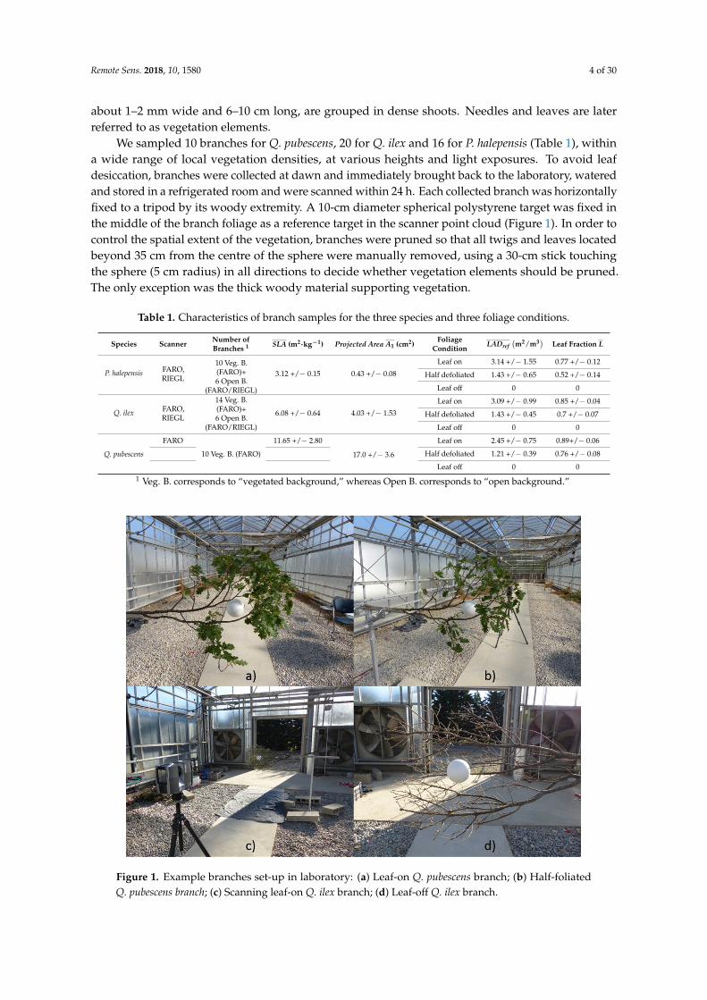
Table 3. Calibration coefficients for LADraw (Equation (9)) and mean absolute percentage error (MAPE)of the corresponding models.

AttenuationCoefficient Voxel Size (m) α (FARO and

RIEGL)[β1; β2; β3](Equation (8))

(FARO Only) MAPE FARO (%) MAPE RIEGL(%)

CF

0.09 1.15 +/− 0.04 [0.6090; 0.8746;−0.3122]P. halepensis: 22.5Q. ilex: 19.7Q. pubescens: 19.1

21.116.7

-

0.7 2.25 +/− 0.09 [0.7311; 0.5314;−0.2614]P. halepensis: 20.4Q. ilex: 25.1Q. pubescens: 21.8

17.119.4

-

Λ̂2

0.09 0.81 +/− 0.04 [0.5141;1.1216;−0.3362]P. halepensis: 24.6Q. ilex: 21.9Q. pubescens: 27.9

25.117.9

-

0.7 1.85 +/− 0.07 [0.6614;0.6765;−0.2623]P. halepensis: 20.6Q. ilex: 22.8Q. pubescens: 19.4

16.815.1

-

Λ̃

0.09 0.76 +/− 0.05 [0.5040;1.0268;−0.3140]P. halepensis: 27.1Q. ilex: 24.2Q. pubescens: 30.8

21.013.9

-

0.7 1.75 +/− 0.07 [0.6873;0.6093;−0.2535]P. halepensis: 20.6Q. ilex: 22.1Q. pubescens: 18.7

16.315.9

-

NB. The (small) distance effect of the RIEGL scanner was neglected (i.e., β1 = 1 and β2 = 0 in Equation (8)).

The calibrated models arising from the most sophisticated attenuation coefficient estimators(Λ̂2 and Λ̃ ) exhibited slightly lower errors than the model deriving from the basic contact frequencyfor the largest voxel size (70 cm) but differences were generally small. When shifting to the smallvoxel size (9 cm), the errors of the FARO scanner increased for estimators derived from Λ̂2 and Λ̃ andremained stable for the contact frequency (CF). Results were more contrasted with the RIEGL scanner,since errors were stable for Q. ilex but increased with P. halepensis when decreasing voxel size.

Overall, the most sophisticated estimators did not perform better than the basic contact frequency(with the exception of the Q. ilex with the RIEGL scanner and the small voxel). This result, which mayseem counterintuitive, could be explained by the fact that unbiased estimators often exhibit a largervariability than simpler biased estimators [15], resulting in some cases to a lower residual error atthe scale of individual measurements (bias-variance trade-off). This crucial point is discussed in thenext section.

Fitting the models on subsets corresponding to species and/or scanners enabled to reduce MAPEvalues by around 5%. However, corresponding models required a much higher number of coefficientsand were thus not considered for further analysis.

Figure 8 shows LAD predictions after calibration (LADcal) for some of the models presented inTable 3. Residual biases of calibrated estimates were low for the FARO instrument, whatever the speciesor the resolution, with the exception of the branches with highest densities, which were generallyunderestimated. This underestimation was explained by the fact that the correction for the distanceeffect was too high in dense branches, because the sensitivity to voxel density of the distance effectwas neglected in the calibration model, as explained in Section 3.3. The RIEGL instrument appeared tobe more prone to overestimations. This is consistent with the fact that no correction was applied forthe positive bias associated with distance in the case of the RIEGL instrument.

Remote Sens. 2018, 10, 1580 18 of 30

Remote Sens. 2018, 10, x FOR PEER REVIEW 18 of 30

appeared to be more prone to overestimations. This is consistent with the fact that no correction was applied for the positive bias associated with distance in the case of the RIEGL instrument.

Figure 8. Reference measurements against calibrated estimators derived from for the three species for (a) P. halepensis with 0.09 cm voxel and FARO scanner; (b) Pinus halepensis with 0.09 m voxel and RIEGL scanner; (c) Q. ilex with 0.09 m voxel and FARO scanner; (d) Q. ilex with 0.09 m voxel and RIEGL scanner; (e) Q. pubescens with 0.09m voxel and FARO scanner; (f) Q. pubescens with 0.09 m voxel and FARO scanner. This figure shows how some of calibration models presented in Table 3 performed against reference measurements.

Figure 8. Reference measurements against calibrated estimators LADcal derived from λCF for the threespecies for (a) P. halepensis with 0.09 cm voxel and FARO scanner; (b) Pinus halepensis with 0.09 m voxeland RIEGL scanner; (c) Q. ilex with 0.09 m voxel and FARO scanner; (d) Q. ilex with 0.09 m voxel andRIEGL scanner; (e) Q. pubescens with 0.09m voxel and FARO scanner; (f) Q. pubescens with 0.09 m voxeland FARO scanner. This figure shows how some of calibration models presented in Table 3 performedagainst reference measurements.

4. Discussion

The present work aimed at providing new insights regarding the measurement of leaf area withTLS, from a comparison with destructive laboratory measurements. Our experimental set-up wasdesigned to investigate the impact of several factors affecting LAD estimations through voxel-basedmethods, which are still poorly understood.

Remote Sens. 2018, 10, 1580 19 of 30

Overall, we observed a strong correlation between the different estimates for LAD and referencemeasurements. However, these relations were found to be dependent on the type of theoreticalestimator (“raw” estimator), the voxel size, the distance to scanner, the scanner type and in alesser extent, the species. The predictions of the LAD raw estimators were corrected thanks toempirical calibrations.

4.1. Raw Estimations of the LAD

Our results showed that the predictions were sensitive to the type of estimator of the attenuationcoefficient. First, we confirmed that the Contact Frequency estimator was negatively biased, at least forshort distance to the scanner, as already reported by [20] from measurements, suggested by [12]and theoretically demonstrated by [15]. However, we point out that such bias can be largelyoverwhelmed by the negative bias associated with large voxels, which might explain the resultsobtained in Reference [20], who used large voxels (2 m). Second, we found that most bias correctionssuggested by [15] were only significant for very small voxels (<9 cm) and long distances (d > 10 m).In these cases, estimators implementing bias corrections exhibited smaller overestimations and highercorrelations with reference measurements than the uncorrected estimators, especially the ModifiedContact Frequency. This result was promising for further applications of these corrections in the field,where occlusion—which was very limited in our laboratory experiment—leads to numerous voxelswhich are sampled by a small number of beams, even at short distance to the scanner, especially whenfine grids are used for scene discretization (i.e., small voxels).

With the exception of these extreme cases, all raw estimators performed similarly once calibrated,including the Contact Frequency. In particular, our analysis showed a linear relationship betweenthe reference measurements and the Contact Frequency and thus the RDI (because the mean freepath is expected to be constant with vegetation density). Such a finding, already reported by [14]in forestry plots, was somehow counterintuitive, as the response function of the LAD to the RDI isexpected to follow the Beer-Lambert law (≈ − log(1− RDI)), which is not linear. This departurefrom the Beer-Lambert law—which assumes a random distribution of vegetation elements within avoxel—could indicate that the organization of plant elements at small scale would not be random butwould rather exhibit some regularity. Indeed, the fact that the absorption (i.e., RDI) was proportionalto the leaf area suggests that element clumps tend to be regularly distributed and that self-shadingis limited. Hence, this result suggests that TLS voxel-based methods can provide critical data toimprove our understanding of plant organization at small scale, which is critical in the context of lightinterception and transpiration modelling [1–3]. It should be recognized, however, that branches werenot scanned under a specific orientation (i.e., from above), meaning that scanner beams do not meetthe actual direct sun exposure pattern inside vegetation, which limits the interpretation in terms oflight interception.

4.2. A Strong Sensitivity of LAD Prediction to Voxel Size, Which Could Mostly Arise from VegetationElement Distribution

The first calibration step (on short-distance measurements) accounted for remaining sourcesof biases and uncertainties, once the distance to scanner and voxel sizes were fixed, namely leaforientation, species, detection capacity of TLS instruments with regards to vegetation structure (beamdiameter, element reflectance, sensor sensitivity, partial hit and mixed points). The resulting calibrationcoefficient was mostly affected by the voxel size. The other factors, such as the species, the instrumentor the type of background, were of secondary importance and often not significant. Such a sensitivityto voxel size was already reported in References [19,20,22].

The bias corrections for element size described in Reference [15] slightly reduced this sensitivitywhen voxel were very small (5–9 cm), when compared to uncorrected estimators. Such findingwas in agreement with [22] who described similar element-size effects in small voxels (<10 cm).However, this sensitivity remained strong for both scanners, all species and all estimators, even when

Remote Sens. 2018, 10, 1580 20 of 30

theoretical bias corrections were included. This hence supports the assumption that the effect of thevoxel size and the subsequent underestimation of LAD observed in largest voxels arose most likelyfrom vegetation heterogeneity, as it was the last remaining source of (negative) bias identified atfixed distance to scanner. It should be noted that [29] found, on the contrary, that LAD predictionsincreased with voxel size, with variations from 1 to 10 in integrated LAD predictions using thevoxel-based canopy profiling method (VCP). This finding can largely be explained by the fact that theVCP method assimilates voxels containing at least one hit to “fully-vegetated” voxels, neglecting theactual vegetation densities in these voxels. As a consequence, the increase in predictions with voxelsize observed in Reference [29] may simply arise from a coarser discretization of vegetated volumes. Itthus cannot be compared to the voxel-based approaches used in the present paper, as they explicitlyaccounted for the vegetation density inside voxels.

Noteworthy, it appeared that the short-distance calibration factors reported in the present studywere remarkably stable among scanners and backgrounds. Also, this stability holds among species,even for the coniferous species, once a rigorous projection of the pine needles was applied (Appendix A).This suggests that these calibration factors could be used in other studies, provided that the leafmorphology and the TLS instrument did not exhibit large differences with those of the present study.

Finally, this potentially critical influence of vegetation distribution on LAD prediction highlightsthe problem of methods based on gap fraction, which generally assume that the vegetation distributionis homogeneous in a horizontal layer, to inverse the transmission equation [10,11,30]. Hence, suchan approach is theoretically equivalent to the application of a voxel-based method to thin “pancake”voxels with a horizontal extent which encompasses the forest plot, thus potentially leading toLAD underestimations.

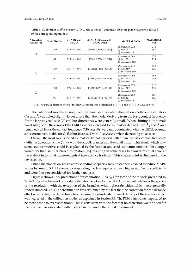
4.3. The Sensitivity to Distance to Scanner Led to the Notion of Effective Footprint and Revealed the Existenceof Spatial Bias in LiDAR Plot-Scale Estimations

In addition to these variations at 2.5 m, a strong effect of distance was revealed for the FAROinstrument and in a smaller extent for the RIEGL instrument. The farther the scanner was from thevegetation, the higher the estimated LAD was. We would like to highlight the importance of thisfinding, which reveals the presence of equally large spatial biases in measurements at the scale of avegetation scene (e.g., forest plot) when raw estimates are not corrected for the distance effect, which isthe case of most studies. Indeed, plot-scale or tree-scale measurements combine various estimationsdone at several distances to scanner, especially when the canopy is high. As a result, an estimated LAIof 2 in a 5-m or in a 20-m high canopy might correspond to considerably different actual LAI. As for thevoxel-size effect, such a distance effect also leads to bias in gap fraction estimates, as their computationrely on the same theoretical basis. Hence, they should also be corrected for distance effect.

As explained in the introduction, this distance effect could be explained by an increase in thehit probability resulting from the increase of laser footprint with distance to scanner, induced bybeam divergence ([12]). Indeed, when beam diameters increase with distance to scanner, beams losetheir ability to pass through vegetation elements without triggering a hit, leading to higher RDI andhence, LAD estimates (Figure 9). In other word, vegetation elements are “seen” by the scanner biggerthan they actually are, as returns can be registered even when the beam centre lines do not interceptany elements. Another explanation to the sensitivity to distance might have been the decay of beamnumber in voxels, which causes a positive theoretical bias in uncorrected estimates [15]. However, weobserved similar increases with distance when this theoretical bias was corrected, suggesting that thebeam divergence was the main cause of observed sensitivity to distance. The distance effect was foundto slightly vary among species (Figure 7), the effect being stronger for species with smaller vegetationelements (pine needles) than with larger leaves. This was consistent with the above explanation,as the relative increase in probability of interception was found to be bigger for fine than for largeelements. The specifications provided by the instrument manufacturers entail to estimate a theoreticalfootprint at the exit (beam diameters equal to 6.5 mm and 2.25 mm for the RIEGL and the FARO,

Remote Sens. 2018, 10, 1580 21 of 30

respectively) and at further distances (beam divergence equal to 0.35 mrad and 0.19 mrad for theRIEGL and the FARO, respectively). From these theoretical specifications, the footprint of the RIEGL at2.5 m (42.7 mm2) should be much larger than the one of the FARO (5.8 mm2), so that the raw estimatesof the FARO should have been much lower than those of the RIEGL. This contradicts the resultsobserved at 2.5 m (calibration coefficient not being sensitive to the instrument) and suggests that theraw estimates do not only reflect the size of the theoretical footprint but also other characteristics ofthe scanner and how beams interact with vegetation elements (element reflectance, sensor sensitivity,partial hit management).

Remote Sens. 2018, 10, x FOR PEER REVIEW 21 of 30

explanation, as the relative increase in probability of interception was found to be bigger for fine than for large elements. The specifications provided by the instrument manufacturers entail to estimate a theoretical footprint at the exit (beam diameters equal to 6.5 mm and 2.25 mm for the RIEGL and the FARO, respectively) and at further distances (beam divergence equal to 0.35 mrad and 0.19 mrad for the RIEGL and the FARO, respectively). From these theoretical specifications, the footprint of the RIEGL at 2.5 m (42.7 mm2) should be much larger than the one of the FARO (5.8 mm2), so that the raw estimates of the FARO should have been much lower than those of the RIEGL. This contradicts the results observed at 2.5 m (calibration coefficient not being sensitive to the instrument) and suggests that the raw estimates do not only reflect the size of the theoretical footprint but also other characteristics of the scanner and how beams interact with vegetation elements (element reflectance, sensor sensitivity, partial hit management).

In practice, a beam diameter of a given size does not mean that a scanner can detect vegetation within this whole footprint. Indeed, a hit is registered only when the intensity of the return is higher than a given threshold [11], so that not all partial hits are detected. To facilitate data interpretation, we suggest the notion of effective footprint (or equivalently effective beam size), which would be the mean footprint area within which vegetation elements are actually detected in a given voxel. This effective footprint would depend of the beam diameter but also of the sensor detection threshold, the return intensity and vegetation element properties and is expected to be smaller than the actual footprint of the scanner. Our short-distance analyses suggest that both the FARO and the RIEGL exhibited similar effective footprints at d = 2.5 m, since the calibration coefficient obtained with both instruments were similar, despite of the differences in theoretical footprints (possibly because of a lower detection threshold of the RIEGL, which might have offset its larger footprint). The distance effect pattern suggested that the effective footprint of the RIEGL was more or less constant with distance up to 10 m, before slightly increasing at further distances. Conversely, the effective footprint of the FARO strongly increased before 10 m and was constant at further distances. A physical modelling of such an effective footprint is not straightforward, even if some physical bases were provided in Reference [11]. However, the physical approach is limited with scanner such as the FARO, as several factors affect the registered value of phase-shift scanner intensity, such as temperature [31] and shooting direction in the different phases. The methodology presented here provided a promising alternative to calibrate the sensitivity to distance.

Figure 9. Impact of the size of the effective footprint on RDI estimates. The increase in effective footprint (blue circles) associated with longer distance to scanner (RDI increasing from 2/9 to 4/9).

The magnitude of the distance effect decreases with voxel size (Figure 7), which was somehow counterintuitive. This observation could arise from the heterogeneous structure of the vegetation, as suggested by the following mechanism. Smaller voxels lead to more frequent “empty” voxels, as their size approaches the size of gaps between shoots in a branch. Hence, the raw LAD distribution is wider on a finer grid. As shown in Appendix E, the distance effect was much stronger in voxels with low density, whereas it was smaller and fairly constant at medium and high densities. As a result, the changes in raw LAD distribution due to smaller voxels (in particular the increase in frequency of low

Figure 9. Impact of the size of the effective footprint on RDI estimates. The increase in effectivefootprint (blue circles) associated with longer distance to scanner (RDI increasing from 2/9 to 4/9).

In practice, a beam diameter of a given size does not mean that a scanner can detect vegetationwithin this whole footprint. Indeed, a hit is registered only when the intensity of the return is higherthan a given threshold [11], so that not all partial hits are detected. To facilitate data interpretation, wesuggest the notion of effective footprint (or equivalently effective beam size), which would be the meanfootprint area within which vegetation elements are actually detected in a given voxel. This effectivefootprint would depend of the beam diameter but also of the sensor detection threshold, the returnintensity and vegetation element properties and is expected to be smaller than the actual footprintof the scanner. Our short-distance analyses suggest that both the FARO and the RIEGL exhibitedsimilar effective footprints at d = 2.5 m, since the calibration coefficient obtained with both instrumentswere similar, despite of the differences in theoretical footprints (possibly because of a lower detectionthreshold of the RIEGL, which might have offset its larger footprint). The distance effect patternsuggested that the effective footprint of the RIEGL was more or less constant with distance up to10 m, before slightly increasing at further distances. Conversely, the effective footprint of the FAROstrongly increased before 10 m and was constant at further distances. A physical modelling of such aneffective footprint is not straightforward, even if some physical bases were provided in Reference [11].However, the physical approach is limited with scanner such as the FARO, as several factors affect theregistered value of phase-shift scanner intensity, such as temperature [31] and shooting direction in thedifferent phases. The methodology presented here provided a promising alternative to calibrate thesensitivity to distance.

The magnitude of the distance effect decreases with voxel size (Figure 7), which was somehowcounterintuitive. This observation could arise from the heterogeneous structure of the vegetation,as suggested by the following mechanism. Smaller voxels lead to more frequent “empty” voxels,as their size approaches the size of gaps between shoots in a branch. Hence, the raw LAD distributionis wider on a finer grid. As shown in Appendix E, the distance effect was much stronger in voxelswith low density, whereas it was smaller and fairly constant at medium and high densities. As a result,the changes in raw LAD distribution due to smaller voxels (in particular the increase in frequencyof low density voxels) induce a higher frequency of voxels with stronger distance effect and hence aslightly stronger overall distance effect (at branch scale) with small voxels.

Remote Sens. 2018, 10, 1580 22 of 30

4.4. Calibrated Estimator Performance

Overall, calibrated raw LAD estimates exhibited lower error with the RIEGL than with the FAROscanner. Hence, the RIEGL obtained the lowest errors with Q. ilex for all voxel sizes (about 15%).The better performance of the RIEGL instrument (despite no correction for distance was applied) mightbe explained by a better management of mixed pixels and a lower level of noise with time-of-flightthan with phase-shift scanners. Indeed, the RIEGL scanner registers the 3D coordinates of the locationwhere the return intensity was the highest, whereas the FARO scanner combines the informationarising from multiple phase shifts (3 wavelengths for the FARO), leading to the registration of a hitposition located within the shortest and longest distances at which intensity was returned, which doesnot necessarily correspond to the location where the actual vegetation element is. Hence, the FAROmight be more subject to hit misplacement. However, the performance of the RIEGL scanner wasgenerally lower with P. halepensis compared to the FARO scanner, especially for the smallest voxelsizes (<15 cm).

Overall, with the exception of Q. ilex, a decrease in voxel size led to higher errors in LADpredictions with both scanners, even with theoretically TBC estimators (Table 3). It has beendemonstrated [15] that the variability in raw estimates sharply increased with decreasing numberof beams and number of vegetation elements within a voxel, leading to large measurements errors.The increase in errors observed below 10 cm suggests that the overall measurement accuracy at branchscale was affected by the measurement errors resulting from random effects occurring at small scale.Indeed, 10 cm appeared as a good compromise between limited error arising from uncertainties ofmeasurements in small voxels and an adequate representation of spatial heterogeneity. It is importantto notice, however, that similar measurement error can be achieved in larger voxels, provided that arelevant calibration was applied.

The lower performance of the more sophisticated (TBC) estimators when applied to the FAROscanner at small voxel size suggests that these estimators were more sensitive to measurement errorand noise than simple estimators (i.e., CF). This could be interpreted as an example of the bias-variancetrade-off. Indeed, sophisticated estimators were theoretically unbiased, meaning that their expectationover a large number of trials was closer to the actual value. [15] showed that their variance was thesmallest that could be expected from any unbiased estimators (since they reached the Cramer-Raobound, see [15]) but also that this variance was high (leading to 95% confident interval as large as100% of the expectation when beam number was low and vegetation elements were large). Moreover,the TBC estimators do not account for vegetation heterogeneity, a major source of bias as suggested inthe present paper. As a result, it is not surprising that once calibrated at the scale of interest (here thebranch), more basic estimators with smaller variance (such as the basic contact frequency approach)were more robust to noise and led to smaller errors than the TBC estimator. Another potential cause oflimited performance of the bias-corrected estimator, might be the fact that the spatial arrangement ofvegetation would not be random at small scale, as suggested in Section 4.1.

These findings, based on detailed laboratory data, highlight the critical need for detailed fielddata and actual TLS data to validate or invalidate finding arising from theory and simulations.

4.5. Recommendations and Further Work

Our study confirmed a strong sensitivity of the LAD estimation to discretization arising fromvegetation heterogeneity and revealed a strong distance effect which, if not corrected, can lead tolarge spatial biases in LiDAR plot-scale estimates. The observed variations among tested scannersshowed that emission pattern and properties of beams from LiDAR instruments play an importantrole in results and in spatial robustness of estimators. We thus recommend that these mechanisms areaccounted for in further studies addressing the estimation of LAD with TLS. These recommendationsapply not only to voxel-based methods but also to gap fraction approaches.

The method presented in the present study (calibration based on experimental tests on branches)could be applied to other species, estimators and instruments as a first step to improve LAD estimations

Remote Sens. 2018, 10, 1580 23 of 30

by the use of calibration functions. The evaluation/calibration procedure developed in this study canbe replicated because it is easily reproducible and reasonably time-consuming (1 week per species).In addition, the same calibration could be applied to species exhibiting close vegetation structure. Thismethod can be seen as a fast approach to characterize bias occurring in LAD estimations.

It is however important to recognize that such laboratory studies do not replace experimentalapproaches at plant [12] or stand scales [14], as additional issues, such as determining the leaf fractionor accounting for occlusion should be tackled to assess reliable LAD [19]. Occlusion was avoided onpurpose in this study to ensure detection of vegetation elements and achieve corrections of biasesrelated to vegetation heterogeneity and scanner properties only. The occurrence of occlusion on fieldmight hence limit reliability of our estimations, even though this work deals with some occlusionissues. Indeed, tested TBC estimators theoretically account for decrease in number of beams usedfor voxel sampling, which is a major drawback of occlusion. In addition, small voxel sizes used inthis study (e.g., 0.09 m) enable an accurate pinpointing of potentially occluded areas. Nevertheless,other biases (i.e., heterogeneous sampling of voxel or totally occluded areas inside tree crowns) are notaddressed as it was not the purpose of this work. Large scale specific experiments at tree or stand scaleare also required to evaluate the calibration derived from laboratory experiments.

Finally, the RIEGL scanner was used in this experiment similarly as a single return instrument,that is, neglecting further impacts (second, third and fourth returns) which only represent 4% oftotal registered returns. This low percentage of multiple returns was mainly due to the backgroundcharacterized by an obstacle-free distance of at least 100 m in the scan direction when the RIEGLscanner was used (see Section 2.1). However, in field measurements, a significant increase in thenumber of multiple returns is expected due to the surrounding vegetation. Considering first returnsonly results in an underestimation of voxel transmittance, that is, an overestimation of RDI and LAD.Indeed, in that case, for each return, the vegetation is implicitly assumed to fully intercept the laserbeam or, in other words, to cover the whole beam area. Most of the time, part of the beam energy is notintercepted and the leaf area responsible for an echo detection is smaller than the whole footprint area.It has been demonstrated that using multiple returns information enhanced LAD estimates and that thesmaller the leaves, the more significant the improvement is [13]. To take into account this informationseveral strategies have been proposed to weight echoes when computing the RDI. Weighting can bebased either on echo intensities [19] or on the number [13] or on the number and rank [32], of theechoes belonging to the same laser beam. However, taking into account partial interceptions remainschallenging due to the numerous factors that influence echo intensity and also because informationabout the amount of energy remaining in the laser beam after the last echo, if any, is always missing.

When dealing with partial interceptions by using multiple returns information, raw LAD estimatesand, consequently, appropriate calibration coefficients can thus depend on voxel environment.For these reasons, it should be more effective and accurate to assess and use the calibrationcoefficients obtained with the proposed approach, considering first returns only when working withfield measurements.

5. Conclusions

This work consolidates and extends previous knowledge regarding the use of TLS to retrievereliable LAD (and LAI) estimates. From our laboratory experiments, we tested recent theoreticaldevelopments regarding the estimation of LAD through voxel-based approaches and identified someimportant sources of bias in measurements. Our analyses permitted to disentangle the biases arisingfrom sampling, vegetation arrangement and scanner specifications. We provided evidences that themost significant biases arose from both the distribution of vegetation element at small scale (voxel-sizeeffect) and some variations in the effective footprint of scanners (distance effect). This “effectivefootprint” is the footprint of a beam in which specific vegetation elements can effectively be detectedat a given distance to scanner. Even for theoretically unbiased estimators, the correction of these

Remote Sens. 2018, 10, 1580 24 of 30

effects was shown to be mandatory and provided LAD estimates within 20% error to the destructivereferences of the present experiment.

Regarding the appropriate voxel size, our study showed that the voxels smaller than 10 cm ledto increasing measurement errors (because of random processes occurring below this scale) and thatthese measurements errors were fairly constant for larger voxel size, provided that an appropriatecalibration coefficient was applied.

We provided a method for the calibration of theoretical estimators. Because tested TLS are widelyused on field campaign on similar vegetation and because measurements at tree scale encompassvoxels at various distances from scanner, this method provides LAD estimates that are less biased whenapplied at plant or plot scale in the field. Calibration functions can be readily applied when vegetationand TLS are similar to those of the present study but should be used with caution in other cases.

Author Contributions: M.S., F.P. and J.-L.D. conceived and designed the experiments; M.S. performed theexperiments, with the help of INRA technical staff, as well as the analyses, with useful guidelines of F.P., J.-L.D.and S.D.; M.S. wrote the paper, with critical contributions of the other co-authors.

Funding: This research was funded by Institut National de la Recherche Agronomique (INRA) and byConseil Régional Provence-Alpes-Côte d’Azur (LiDARForFuel, grant n◦ APR-EX 2014_04163 and PhD grant n◦2015_07468). The APC was funded by INRA.

Acknowledgments: The authors would like to thanks Maxence Carra, Frederic Jean, Philippe Petit and DenisPortier for support in defoliating process, and measurements of destructive references, such as total leaf areaand SLA. The authors are also grateful to Christian Pichot who provided GRASS routine for identification of leafpixels in 2D flat scans. The authors also thank Jean-Paul Douzals for providing an appropriate facility for TLSmeasurements in IRSTEA Montpellier. The authors thank Office national des forêts and Chateau de Javon for allowingto collect branches in stands.

Conflicts of Interest: The authors declare no conflict of interest. The founding sponsors had no role in the designof the study; in the collection, analyses, or interpretation of data; in the writing of the manuscript and in thedecision to publish the results.

Appendix A

For a mass M of flat leaves (with individual mass M1, projected area A1 and radius r),the corresponding one-sided leaf area LA (half total area of foliage) is the following function ofthe (projected) SLA:

LA(m2) =12

MM1

2πr2 = Mπr2

M1= M

A1

M1= M

As

Ms= M SLA (A1)

For a mass M of cylindrical needles (with individual mass M1, projected area A1, radius r andlength l), the corresponding one-sided leaf area LA (half total area of foliage) is the following functionof the (projected) SLA:

LA(m2) =12

MM1

2πrl =π

2M

2rlM1

=π

2M

A1

M1=

π

2M

As

Ms=

π

2M SLA (A2)

Following the definition of λ1, it leads for a flat leaf of radius r to:

λ1 =S1

V=

Stot

4V=

2πr2

4V=

2A1

4V=

A1

2V=

As

2Vns. (A3)

For a needle of radius r and length l, this leads to:

λ1 =S1

V=

Stot

4V=

2πrl4V

=πA1

4V=

πAs

4Vns(A4)

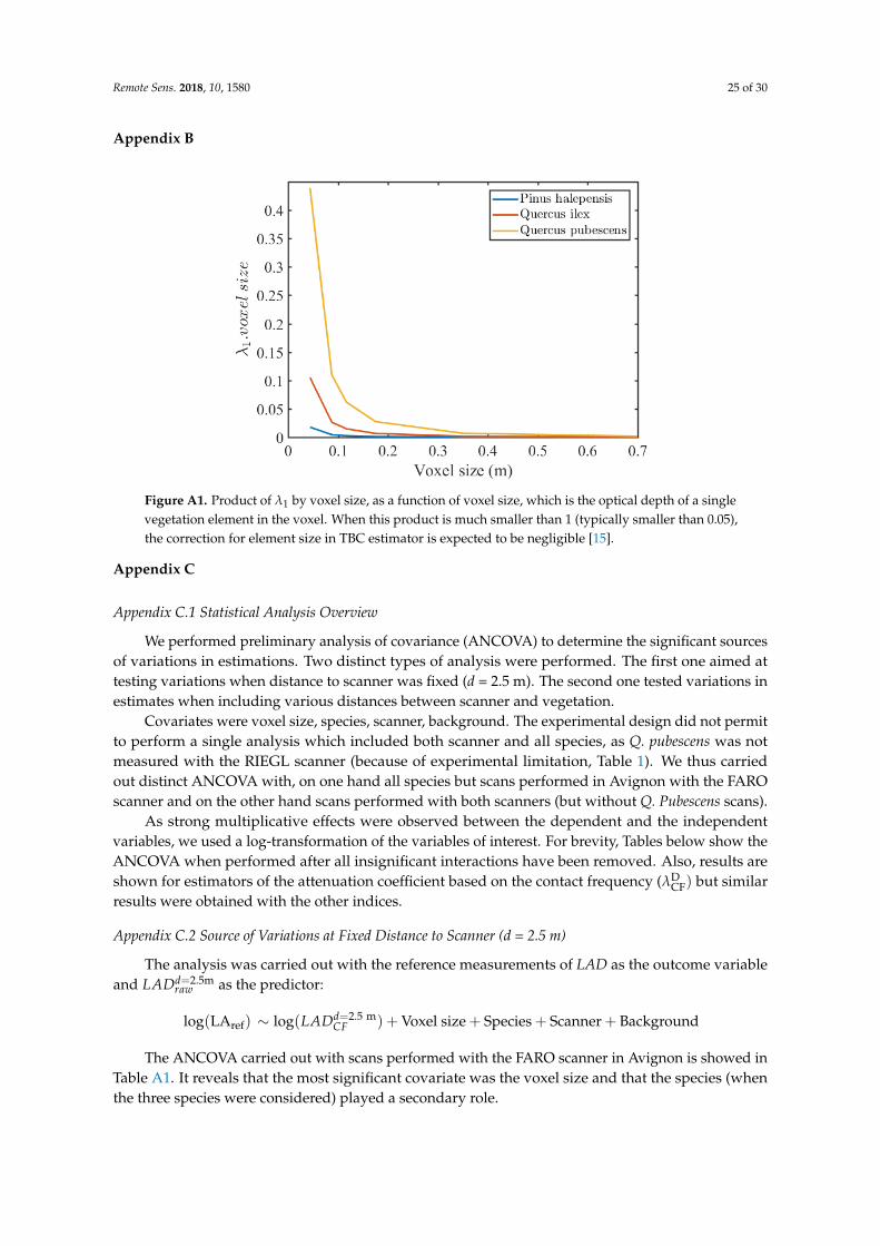
Remote Sens. 2018, 10, 1580 25 of 30

Appendix BRemote Sens. 2018, 10, x FOR PEER REVIEW 25 of 30

Appendix B

Figure A1. Product of by voxel size, as a function of voxel size, which is the optical depth of a single vegetation element in the voxel. When this product is much smaller than 1 (typically smaller than 0.05), the correction for element size in TBC estimator is expected to be negligible [15].

Appendix C

Appendix C1. Statistical Analysis Overview

We performed preliminary analysis of covariance (ANCOVA) to determine the significant sources of variations in estimations. Two distinct types of analysis were performed. The first one aimed at testing variations when distance to scanner was fixed (d = 2.5 m). The second one tested variations in estimates when including various distances between scanner and vegetation.

Covariates were voxel size, species, scanner, background. The experimental design did not permit to perform a single analysis which included both scanner and all species, as Q. pubescens was not measured with the RIEGL scanner (because of experimental limitation, Table 1). We thus carried out distinct ANCOVA with, on one hand all species but scans performed in Avignon with the FARO scanner and on the other hand scans performed with both scanners (but without Q. Pubescens scans).

As strong multiplicative effects were observed between the dependent and the independent variables, we used a log-transformation of the variables of interest. For brevity, Tables below show the ANCOVA when performed after all insignificant interactions have been removed. Also, results are shown for estimators of the attenuation coefficient based on the contact frequency (λ ) but similar results were obtained with the other indices.

Appendix C2. Source of Variations at Fixed Distance to Scanner (d = 2.5 m)

The analysis was carried out with the reference measurements of LAD as the outcome variable and . as the predictor: log(LA )~ log =2.5m + Voxelsize + Species + Scanner + Background

The ANCOVA carried out with scans performed with the FARO scanner in Avignon is showed in Table A1. It reveals that the most significant covariate was the voxel size and that the species (when the three species were considered) played a secondary role.

Figure A1. Product of λ1 by voxel size, as a function of voxel size, which is the optical depth of a singlevegetation element in the voxel. When this product is much smaller than 1 (typically smaller than 0.05),the correction for element size in TBC estimator is expected to be negligible [15].

Appendix C

Appendix C.1 Statistical Analysis Overview

We performed preliminary analysis of covariance (ANCOVA) to determine the significant sourcesof variations in estimations. Two distinct types of analysis were performed. The first one aimed attesting variations when distance to scanner was fixed (d = 2.5 m). The second one tested variations inestimates when including various distances between scanner and vegetation.

Covariates were voxel size, species, scanner, background. The experimental design did not permitto perform a single analysis which included both scanner and all species, as Q. pubescens was notmeasured with the RIEGL scanner (because of experimental limitation, Table 1). We thus carriedout distinct ANCOVA with, on one hand all species but scans performed in Avignon with the FAROscanner and on the other hand scans performed with both scanners (but without Q. Pubescens scans).

As strong multiplicative effects were observed between the dependent and the independentvariables, we used a log-transformation of the variables of interest. For brevity, Tables below show theANCOVA when performed after all insignificant interactions have been removed. Also, results areshown for estimators of the attenuation coefficient based on the contact frequency (λD

CF) but similarresults were obtained with the other indices.

Appendix C.2 Source of Variations at Fixed Distance to Scanner (d = 2.5 m)

The analysis was carried out with the reference measurements of LAD as the outcome variableand LADd=2.5m

raw as the predictor:

log(LAref) ∼ log(LADd=2.5 mCF ) + Voxel size + Species + Scanner + Background

The ANCOVA carried out with scans performed with the FARO scanner in Avignon is showed inTable A1. It reveals that the most significant covariate was the voxel size and that the species (whenthe three species were considered) played a secondary role.

Remote Sens. 2018, 10, 1580 26 of 30

Table A1. ANCOVA of log (LADre f ) for scans carried out with the FARO scanner in Avignon (all species).

Effects D.F. F-Value p-Value

Intercept 1 272 2.2× 10−16

Log (LADd=2.5mCF ) 1 349.0 2.2× 10−16

log (LADd=2.5mCF ):voxel size 5 17.1 2.6× 10−15

log (LADd=2.5mCF ):species 2 4.37 0.01

Only the significant factors are presented.

When a similar ANCOVA was carried out with both scanners (but without Q. Pubescens), the speciesdid not show up as significant, which confirms that the species was of secondary importance (Table A2).

Table A2. ANCOVA of log(

LADre f

)for all scans except those of Q. Pubescens.

Effects D.F. F-Value p-Value

Intercept 1 756.6 2.2× 10−16

Log (LADd=2.5mCF ) 1 155.1 2.2× 10−16

log (LADd=2.5mCF ):voxel size 5 10.5 1.7× 10−9

Only the significant factors are presented.

In both analyses, the raw estimates of LAD were the main variable explaining the LADre f .The interaction with voxel size was found significant. The interaction with species was of secondaryimportance. The type of scanner and background were never found significant, which establishes themain contribution of voxel size, at a given distance.

Appendix C.3 Source of Variations in Predictions When Distance to Scanner Varies

The analysis was carried out with the raw LAD estimates at d = 2.5 m as the outcome variable andLADd

raw as the predictor:

log(LADd=2.5mCF ) ∼ log(LADd

CF) + Voxel size + Species + Scanner + Background

The ANCOVA carried out with scans performed with the FARO scanner in Avignon is showed inTable A3. It reveals that the most significant covariate was the distance to scanner, which exhibitedsignificant interactions with both voxel size and species. In particular, the distance effect for Q. pubescensdiffered from the one of two other species. These interactions, however, explained much less of thetotal variance, than the main factors (i.e., F-Values are much smaller than for Log(LADd

CF) and distanceto scanner).

Table A3. ANCOVA of log(LADd=2.5mCF ) for scans carried out with the FARO scanner in Avignon (all

species).

Effects D.F. F-Value p-Value

Intercept 1 44.0 4.5× 10−11

Log (LADdCF) 1 12990.9 2× 10−16

Distance 1 2317.5 2× 10−16

Distance:voxel size 4 127.6 2× 10−16

Distance:Species 2 358.1 2× 10−16

Only the significant factors are presented.

When a similar ANCOVA was carried out with both scanners (but without Q. Pubescens),the species did not show up as significant, which confirms that the species was of secondary importance(Table A4). The distance was found to be in interaction with the scanner type at a relatively largeF-Value, suggesting that the sensitivity to distance to scanner differed for the two scanners. Such

Remote Sens. 2018, 10, 1580 27 of 30

distance effect analysed separately on RIEGL was found to be statistically minor, suggesting a muchsmaller distance effect on the RIEGL than on the FARO scanner (not shown).

Table A4. ANCOVA of log(LADd=2.5mCF ) for all scans except those of Q. Pubescens.

Effects D.F. F-Value p-Value

Intercept 1 44.3 3.75× 10−11

Log (LADdCF) 1 9663.8 2.2× 10−16

Distance 1 1587.4 2.2× 10−16

Distance:scanner 1 719.6 2.2× 10−16

Distance:voxel size 4 91.2 2.2× 10−16

Only the significant factors are presented.

In both analysis, the raw estimates of LAD at other distances was the main variable explainingthe raw estimates at short distance. We found however, that the distance to scanner was highlysignificant, especially with the FARO scanner. The interaction with species or voxel size was ofsecondary importance. No effect of background was detected.

Appendix D Impact of Bias Correction for Element Size though the “Effective” Mean Free Path

Remote Sens. 2018, 10, x FOR PEER REVIEW 27 of 30

distance effect analysed separately on RIEGL was found to be statistically minor, suggesting a much smaller distance effect on the RIEGL than on the FARO scanner (not shown).

Table A4. ANCOVA of log =2.5m for all scans except those of Q. Pubescens.

Effects D.F. F-Value p-Value Intercept 1 44.3 3.75 × 10

Log( ) 1 9663.8 2.2 × 10 Distance 1 1587.4 2.2 × 10 Distance:scanner 1 719.6 2.2 × 10

Distance:voxel size 4 91.2 2.2 × 10 Only the significant factors are presented.

In both analysis, the raw estimates of LAD at other distances was the main variable explaining the raw estimates at short distance. We found however, that the distance to scanner was highly significant, especially with the FARO scanner. The interaction with species or voxel size was of secondary importance. No effect of background was detected.

Appendix D. Impact of Bias Correction for Element Size though the “Effective” Mean Free Path

Figure A2. Distributions of mean free path and mean effective free path in voxels with two sizes (0.04 m and 0.12 m) of Q. pubescens. (a) Distribution of mean free path lengths ̅ in a 0.04 m voxel; (b) Distribution of mean free path lengths ̅ in a 0.12 m voxel; (c) Distribution of mean “effective” free path lengths in a 0.04 m voxel; (d) Distribution of mean “effective” free path lengths in a 0.12 m voxel. A shift in distribution between (a,c) was observed: values were significantly larger than ̅ values, leading to smaller estimates when the correction for element size is included ( replaced ̅ at the denominator of the corrected estimator, see Table 2). When voxel size was larger (0.12 m), the distributions of ̅ and were almost identical, as shown in (b,d), leading to negligible bias correction.

Figure A2. Distributions of mean free path and mean effective free path in voxels with two sizes(0.04 m and 0.12 m) of Q. pubescens. (a) Distribution of mean free path lengths z in a 0.04 m voxel;(b) Distribution of mean free path lengths z in a 0.12 m voxel; (c) Distribution of mean “effective”free path lengths ze in a 0.04 m voxel; (d) Distribution of mean “effective” free path lengths ze ina 0.12 m voxel. A shift in distribution between (a,c) was observed: ze values were significantlylarger than z values, leading to smaller estimates when the correction for element size is included(ze replaced z at the denominator of the corrected estimator, see Table 2). When voxel size was larger(0.12 m), the distributions of z and ze were almost identical, as shown in (b,d), leading to negligiblebias correction.

Remote Sens. 2018, 10, 1580 28 of 30

Appendix E Impact of the Density of Vegetation on the Distance Effect Observed in IndividualVoxels

Remote Sens. 2018, 10, x FOR PEER REVIEW 28 of 30

Appendix E. Impact of the Density of Vegetation on the Distance Effect Observed in Individual Voxels

Figure A3. Sensitivity to distance to scanner of raw estimates in individual voxels, grouped by classes of estimated densities, expressed by the mean “distance effect ratio” of each class (Equation (7)): (a) Density class 1 (low raw estimates); (b) Density class 2 (low to medium raw estimates); (c)) Density class 3 (medium to high raw estimates); (d)) Density class 4 (high raw estimates). This figure illustrates that the distance effects were much stronger in voxels with low vegetation density that in those of medium to high densities.

References

1. Norman, J.M.; Campbell, G.S. Canopy structure. In Plant Physiological Ecology: Field Methods and Instrumentation; Pearcy, R.W., Ehleringer, J.R., Mooney, H.A., Rundel, P.W., Eds.; Springer: Dordrecht, The Netherlands, 1989; pp. 301–325, ISBN 978-94-009-2221-1.

2. Simioni, G.; Marie, G.; Huc, R. Influence of vegetation spatial structure on growth and water fluxes of a mixed forest: Results from the NOTG 3D model. Ecol. Model. 2016, 328, 119–135, doi:10.1016/j.ecolmodel.2016.02.004.

Figure A3. Sensitivity to distance to scanner of raw estimates in individual voxels, grouped by classesof estimated densities, expressed by the mean “distance effect ratio” of each class (Equation (7)):(a) Density class 1 (low raw estimates); (b) Density class 2 (low to medium raw estimates); (c)) Densityclass 3 (medium to high raw estimates); (d)) Density class 4 (high raw estimates). This figure illustratesthat the distance effects were much stronger in voxels with low vegetation density that in those ofmedium to high densities.

References

1. Norman, J.M.; Campbell, G.S. Canopy structure. In Plant Physiological Ecology: Field Methods andInstrumentation; Pearcy, R.W., Ehleringer, J.R., Mooney, H.A., Rundel, P.W., Eds.; Springer: Dordrecht,The Netherlands, 1989; pp. 301–325. ISBN 978-94-009-2221-1.

2. Simioni, G.; Marie, G.; Huc, R. Influence of vegetation spatial structure on growth and water fluxes of amixed forest: Results from the NOTG 3D model. Ecol. Model. 2016, 328, 119–135. [CrossRef]

3. Vezy, R.; Christina, M.; Roupsard, O.; Nouvellon, Y.; Duursma, R.; Medlyn, B.; Soma, M.; Charbonnier, F.;Blitz-Frayret, C.; Stape, J.L.; et al. Measuring and modelling energy partitioning in canopies of varyingcomplexity using MAESPA model. Agric. For. Meteorol. 2018, 253–254, 203–217. [CrossRef]

4. Vierling, K.T.; Vierling, L.A.; Gould, W.A.; Martinuzzi, S.; Clawges, R.M. Lidar: Shedding new light onhabitat characterization and modeling. Front. Ecol. Environ. 2008, 6, 90–98. [CrossRef]

Remote Sens. 2018, 10, 1580 29 of 30

5. Keane, R. Wildland Fuel Fundamentals and Applications; Springer International Publishing: Cham, Switzerland,2015.

6. Jonckheere, I.; Fleck, S.; Nackaerts, K.; Muys, B.; Coppin, P.; Weiss, M.; Baret, F. Review of methods for in situleaf area index determination Part I. Theories, sensors and hemispherical photography. Agric. For. Meteorol.2004, 121, 19–35. [CrossRef]

7. Bréda, N.J.J. Ground-based measurements of leaf area index: A review of methods, instruments and currentcontroversies. J. Exp. Bot. 2003, 54, 2403–2417. [CrossRef] [PubMed]

8. Weiss, M.; Baret, F.; Smith, G.J.; Jonckheere, I.; Coppin, P. Review of methods for in situ leaf area index(LAI) determination Part II. Estimation of LAI, errors and sampling. Agric. For. Meteorol. 2004, 121, 37–53.[CrossRef]

9. Chen, J.M.; Cihlar, J. Plant canopy gap-size analysis theory for improving optical measurements of leaf-areaindex. Appl. Opt. 1995, 34, 6211–6222. [CrossRef] [PubMed]

10. Jupp, D.L.B.; Culvenor, D.S.; Lovell, J.L.; Newnham, G.J.; Strahler, A.H.; Woodcock, C.E. Estimating forestLAI profiles and structural parameters using a ground-based laser called ’Echidna? Tree Physiol. 2009,29, 171–181. [CrossRef] [PubMed]

11. Zhao, K.; García, M.; Liu, S.; Guo, Q.; Chen, G.; Zhang, X.; Zhou, Y.; Meng, X. Terrestrial lidar remote sensingof forests: Maximum likelihood estimates of canopy profile, leaf area index, and leaf angle distribution.Agric. For. Meteorol. 2015, 209–210, 100–113. [CrossRef]

12. Béland, M.; Widlowski, J.L.; Fournier, R.A.; Cote, J.F.; Verstraete, M.M. Estimating leaf area distribution insavanna trees from terrestrial LiDAR measurements. Agric. For. Meteorol. 2011, 151, 1252–1266. [CrossRef]

13. Grau, E.; Durrieu, S.; Fournier, R.; Gastellu-etchegorry, J.; Yin, T. Estimation of 3D vegetation densitywith Terrestrial Laser Scanning data using voxels. A sensitivity analysis of influencing parameters.Remote Sens. Environ. 2017, 191, 373–388. [CrossRef]

14. Pimont, F.; Dupuy, J.L.; Rigolot, E.; Prat, V.; Piboule, A. Estimating leaf bulk density distribution in a treecanopy using terrestrial LiDAR and a straightforward calibration procedure. Remote Sens. 2015, 7, 7995–8018.[CrossRef]

15. Pimont, F.; Allard, D.; Soma, M.; Dupuy, J.L. Estimators and confidence intervals for plant area density atvoxel scale with T-LiDAR. Remote Sens. Environ. 2018, 215, 343–370. [CrossRef]

16. Durrieu, S.; Allouis, T.; Fournier, R.; Véga, C.; Albrech, L. Spatial quantification of vegetation density fromterrestrial laser scanner data for characterization of 3D forest structure at plot level. In Proceedings of theSilviLaser 2008, Edinburgh, UK, 17–19 September 2008; pp. 325–334.

17. Hosoi, F.; Omasa, K. Factors contributing to accuracy in the estimation of the woody canopy leaf area densityprofile using 3D portable lidar imaging. J. Exp. Bot. 2007, 58, 3463–3473. [CrossRef] [PubMed]

18. Bailey, B.; Mahaffee, W. Rapid, high-resolution measurement of leaf area and leaf orientation using terrestrialLiDAR scanning data. Meas. Sci. Technol. 2017, 28, 6. [CrossRef]

19. Béland, M.; Widlowski, J.L.; Fournier, R.A. A model for deriving voxel-level tree leaf area density estimatesfrom ground-based LiDAR. Environ. Model. Softw. 2014, 51, 184–189. [CrossRef]

20. Bailey, B.N.; Mahaffee, W.F. Rapid measurement of the three-dimensional distribution of leaf orientationand the leaf angle probability density function using terrestrial LiDAR scanning. Remote Sens. Environ. 2017,194, 63–76. [CrossRef]

21. Seielstad, C.; Stonesifer, C.; Rowell, E.; Queen, L. Deriving fuel mass by size class in Douglas-fir (Pseudotsugamenziesii) using terrestrial laser scanning. Remote Sens. 2011, 3, 1691–1709. [CrossRef]

22. Béland, M.; Baldocchi, D.D.; Widlowski, J.L.; Fournier, R.A.; Verstraete, M.M. On seeing the wood fromthe leaves and the role of voxel size in determining leaf area distribution of forests with terrestrial LiDAR.Agric. For. Meteorol. 2014, 184, 82–97. [CrossRef]

23. Ruel, J.J.; Ayres, M.P. Jensen’s inequality predicts effects of environmental variation. Tree 1999, 5347, 361–366.[CrossRef]

24. Pimont, F.; Dupuy, J.L.; Caraglio, Y.; Morvan, D. Effect of vegetation heterogeneity on radiative transfer inforest fires. Int. J. Wildland Fire 2009, 18, 536–553. [CrossRef]

25. Hebert, M.; Krotkov, E. 3D measurements from imaging laser radars: How good are they? Image Vis. Comput.1992, 10, 170–178. [CrossRef]

Remote Sens. 2018, 10, 1580 30 of 30

26. Newnham, G.; Armston, J.; Muir, J.; Goodwin, N.; Tindall, D.; Culvenor, D.; Püschel, P.; Nyström, M.;Johansen, K. Evaluation of Terrestrial Laser Scanners for Measuring Vegetation Structure; CSIRO SustainableAgriculture Flagship; CSIRO: Canberra, Australia, 2012; pp. 1–32. [CrossRef]

27. Leica Geosystems Cyclone Pointcloud Export Format—Description of ASCII. Ptx Format. Availableonline: http://w3.leica-geosystems.com/kb/?guid=5532D590-114C-43CD-A55F-FE79E5937CB2 (accessedon 22 June 2018).

28. Wilson, J.W. Inclined point quadrats. New Phytol. 1960, 59, 1–7. [CrossRef]29. Li, S.; Dai, L.; Wang, H.; Wang, Y.; He, Z.; Lin, S. Estimating leaf area density of individual trees using the

point cloud segmentation of terrestrial LiDAR data and a voxel-based model. Remote Sens. 2017, 9, 1202.[CrossRef]

30. Zhao, F.; Yang, X.; Schull, M.A.; Román-Colón, M.O.; Yao, T.; Wang, Z.; Zhang, Q.; Jupp, D.L.B.; Lovell, J.L.;Culvenor, D.S.; et al. Measuring effective leaf area index, foliage profile, and stand height in New Englandforest stands using a full-waveform ground-based lidar. Remote Sens. Environ. 2011, 115, 2954–2964.[CrossRef]

31. Errington, A.F.C.; Daku, B.L.F. Temperature compensation for radiometric correction of terrestrial LiDARintensity data. Remote Sens. 2017, 9, 356. [CrossRef]

32. Vincent, G.; Antin, C.; Laurans, M.; Heurtebize, J.; Durrieu, S.; Lavalley, C.; Dauzat, J. Mapping plant areaindex of tropical evergreen forest by airborne laser scanning. A cross-validation study using LAI2200 opticalsensor. Remote Sens. Environ. 2017, 198, 254–266. [CrossRef]

© 2018 by the authors. Licensee MDPI, Basel, Switzerland. This article is an open accessarticle distributed under the terms and conditions of the Creative Commons Attribution(CC BY) license (http://creativecommons.org/licenses/by/4.0/).