
Enhanced Bilateral Teleoperation using Generalized...
159
Enhanced Bilateral Teleoperation using Generalized Force/Position Mapping
-
Upload
nguyenliem -
Category
Documents
-
view
220 -
download
2
Transcript of Enhanced Bilateral Teleoperation using Generalized...

Enhanced Bilateral Teleoperation using
Generalized Force/Position Mapping

ENHANCED BILATERAL TELEOPERATION USING
GENERALIZED FORCE/POSITION MAPPING
BY
PAWEL MALYSZ, B.Eng.
A THESIS
SUBMITTED TO THE DEPARTMENT OF ELECTRICAL & COMPUTER ENGINEERING
AND THE SCHOOL OF GRADUATE STUDIES
OF MCMASTER UNIVERSITY
IN PARTIAL FULFILMENT OF THE REQUIREMENTS
FOR THE DEGREE OF
MASTER OF APPLIED SCIENCE
c© Copyright by Pawel Malysz, September 2007
All Rights Reserved

Master of Applied Science (2007) McMaster University
(Electrical & Computer Engineering) Hamilton, Ontario, Canada
TITLE: Enhanced Bilateral Teleoperation using Generalized
Force/Position Mapping
AUTHOR: Pawel Malysz
B.Eng., (Engineering Physics)
McMaster University, Hamilton, Ontario, Canada
SUPERVISOR: Dr. Shahin Sirouspour
NUMBER OF PAGES: xiv, 144
ii

To my family and Araksi

Abstract
The performance index in teleoperation, transparency, is often defined as linear
scaling of force and position between the master/operator and slave/environment.
Motivated by applications involving soft tissue manipulation such as robotic sur-
gery, the transparency objective is generalized in this thesis to include static non-
linear and linear-time-invariant filter mappings between the master/slave posi-
tion and force signals. Lyapunov-based adaptive motion/force controllers are pro-
posed to achieve the generalized transparency objectives. Using Lyapunov stabil-
ity theory the mapped position and force tracking errors are shown to converge in
the presence of dynamic uncertainty in the master/slave robots and user/environ-
ment dynamics. Given a priori known bounds on unknown dynamic parameters,
a framework for robust stability analysis is proposed that uses stability of Lur’e-
Postinkov systems and Nyquist/Bode envelopes of interval plant systems. Meth-
ods for finding the required Nyquist/Bode envelopes are presented in this thesis.
A comprehensive stability analysis is performed under different sets of general-
ized mappings. For nonlinear mapping of either position or force, robust stability
depends on stability of an equivalent Lur’e-Postinikov system. Stability results
of such systems are discussed in this thesis. In particular, the on and off-axis cir-
cle theorems are utilized. Using these theorems, sufficient teleoperation stability
iv
regions are obtained that are far less conservative than those obtained from passiv-
ity. In the special case of LTI filtered force and position mappings the exact robust
stability regions are obtained by showing stability of the relevant closed-loop char-
acteristic polynomial. The proposed robust stability test uses the phase values of a
limited set of extremal polynomials.
To demonstrate the utility of the generalized performance measures, a stiffness
discrimination tele-manipulation task is considered in which the user compares
and contrasts the stiffness of soft environments via haptic exploration in the pres-
ence and absence of visual feedback. Using adaptive psychophysical perception
experiments a nonlinear force mapping is shown to enhance stiffness discrimina-
tion thresholds. The design guidelines for this enhanced nonlinear force mapping
are reported in this thesis. Generalized nonlinear and linear filtered mappings are
achieved in experiments with a two-axis teleoperation system where the details of
implementation are given.
v

Acknowledgements
My thanks and appreciation to my supervisor, Dr. Shahin Sirouspour, for his guid-
ance, support and encouragement throughout my graduate program here at Mc-
Master.
Sincere gratitude to my fellow colleagues in the Haptics, Telerobotics and Com-
putational Vision Lab, Ali Shahdi, Mahyar Fotoohi, Mike Kinsner, Ivy Zhong, Insu
Park, Brian Moody, Sina Niakosari, Bassma Ghali, Saba Moghimi, Ramin Mafi and
Amin Abdossalami for making this a fun and enjoyable place to study as well as
for their help in my research.
Special thanks to my family since they have made it possible for me to excel in
my academic studies with their endless love and support throughout my life. My
deepest love to Araksi, for her unwavering love, patience and support makes me
feel anything is possible.
vi
Contents
Abstract iv
Acknowledgements vi
1 Introduction 1
1.1 Motivation . . . . . . . . . . . . . . . . . . . . . . . . . . . . . . . . . . 1
1.2 Problem Statement and Thesis Contributions . . . . . . . . . . . . . . 4
1.3 Organization of the Thesis . . . . . . . . . . . . . . . . . . . . . . . . . 7
1.4 Related Publications . . . . . . . . . . . . . . . . . . . . . . . . . . . . 7
2 Literature Review 8
2.1 Teleoperation . . . . . . . . . . . . . . . . . . . . . . . . . . . . . . . . 9
2.1.1 Two-port Network Model . . . . . . . . . . . . . . . . . . . . . 9
2.1.2 Teleoperation Control Approaches . . . . . . . . . . . . . . . . 12
2.2 Telesurgery and Soft-tissue Telemanipulation . . . . . . . . . . . . . . 15
2.3 Haptic Perception . . . . . . . . . . . . . . . . . . . . . . . . . . . . . . 18
3 Lyapunov Based Adaptive Controllers 20
3.1 Dynamics of Master/Slave Systems . . . . . . . . . . . . . . . . . . . 21
vii
3.2 Control Design . . . . . . . . . . . . . . . . . . . . . . . . . . . . . . . 24
3.2.1 Local Adaptive Controllers . . . . . . . . . . . . . . . . . . . . 24
3.2.2 Teleoperation . . . . . . . . . . . . . . . . . . . . . . . . . . . . 28
4 Interval Plant Systems 34
4.1 Interval Polynomials . . . . . . . . . . . . . . . . . . . . . . . . . . . . 35
4.1.1 Kharitonov Polynomials . . . . . . . . . . . . . . . . . . . . . . 35
4.1.2 Polytopic Polynomials . . . . . . . . . . . . . . . . . . . . . . . 38
4.2 Kharitonov Plants . . . . . . . . . . . . . . . . . . . . . . . . . . . . . . 44
4.2.1 Bode Envelope . . . . . . . . . . . . . . . . . . . . . . . . . . . 44
4.2.2 Nyquist Envelope . . . . . . . . . . . . . . . . . . . . . . . . . . 46
4.3 Polytopic Plants . . . . . . . . . . . . . . . . . . . . . . . . . . . . . . . 49
4.3.1 Bode Envelope . . . . . . . . . . . . . . . . . . . . . . . . . . . 49
4.3.2 Nyquist Envelope . . . . . . . . . . . . . . . . . . . . . . . . . . 53
5 Stability of Lur’e-Postnikov Systems 56
5.1 Input-Output Passivity . . . . . . . . . . . . . . . . . . . . . . . . . . . 58
5.1.1 Passive and Strictly Passive Systems . . . . . . . . . . . . . . . 58
5.1.2 Passivity Stability Theorem . . . . . . . . . . . . . . . . . . . . 59
5.1.3 Passivity of Linear Systems . . . . . . . . . . . . . . . . . . . . 61
5.2 On-Axis Circle Theorem . . . . . . . . . . . . . . . . . . . . . . . . . . 62
5.2.1 Small Gain Approach . . . . . . . . . . . . . . . . . . . . . . . 62
5.2.2 Loop transformation . . . . . . . . . . . . . . . . . . . . . . . . 63
5.3 Off-Axis Circle Theorem . . . . . . . . . . . . . . . . . . . . . . . . . . 65
5.3.1 Passivity with Multipliers . . . . . . . . . . . . . . . . . . . . . 66
viii

5.3.2 Loop Transformations . . . . . . . . . . . . . . . . . . . . . . . 69
5.4 Other Methods . . . . . . . . . . . . . . . . . . . . . . . . . . . . . . . 72
6 Teleoperation Stability Analysis 74
6.1 Static Nonlinear Feedback . . . . . . . . . . . . . . . . . . . . . . . . . 75
6.1.1 Passivity approach . . . . . . . . . . . . . . . . . . . . . . . . . 75
6.1.2 Circle criterions with Nyquist envelope . . . . . . . . . . . . . 77
6.2 LTI Filtered Mappings . . . . . . . . . . . . . . . . . . . . . . . . . . . 81
6.2.1 Additional force filtering . . . . . . . . . . . . . . . . . . . . . 83
6.2.2 Force compensator mapping . . . . . . . . . . . . . . . . . . . 85
6.2.3 Hand tremor position filter . . . . . . . . . . . . . . . . . . . . 86
6.3 Mixed Non-Linear/LTI Filtered Mappings . . . . . . . . . . . . . . . 88
6.4 Conservatism of using Bode envelopes . . . . . . . . . . . . . . . . . . 90
7 Psychophysics 93
7.1 Psychophysics Theory and Methods . . . . . . . . . . . . . . . . . . . 94
7.1.1 Theory . . . . . . . . . . . . . . . . . . . . . . . . . . . . . . . . 94
7.1.2 Methods . . . . . . . . . . . . . . . . . . . . . . . . . . . . . . . 97
7.2 Enhanced Mapping Design . . . . . . . . . . . . . . . . . . . . . . . . 103
7.2.1 Nonlinear force mapping . . . . . . . . . . . . . . . . . . . . . 103
7.2.2 Nonlinear Spatial and Filtered Mappings . . . . . . . . . . . . 105
7.3 Experiments . . . . . . . . . . . . . . . . . . . . . . . . . . . . . . . . . 107
8 Teleoperation Experiments 113
8.1 Experimental Setup . . . . . . . . . . . . . . . . . . . . . . . . . . . . . 114
8.2 Controller Implementation . . . . . . . . . . . . . . . . . . . . . . . . . 115
ix

8.3 Experimental Results . . . . . . . . . . . . . . . . . . . . . . . . . . . . 120
8.3.1 Nonlinear force scaling with filtered position mapping . . . . 121
8.3.2 Nonlinear position scaling with filtered force mapping . . . . 124
9 Conclusions and Future Work 127
A Appendix 130
A.1 Strict positive realness of G(s) = Ze/(Zh + Zt) . . . . . . . . . . . . . 130
A.2 Repeated Measures ANOVA . . . . . . . . . . . . . . . . . . . . . . . . 132
x

List of Figures
1.1 Teleoperation systems. a) Example system at McMaster University
b) Basic system elements. . . . . . . . . . . . . . . . . . . . . . . . . . 3
2.1 Teleoperation two port network model. Figure from [1]. . . . . . . . . 9
2.2 Teleoperation block diagram. Figure from [1]. . . . . . . . . . . . . . . 11
2.3 System for robust controller synthesis . . . . . . . . . . . . . . . . . . 14
3.1 Teleoperation block diagrams. . . . . . . . . . . . . . . . . . . . . . . 32
4.1 Image sets of Ze = δ2s2 + δ1s + δ0 from ω = 63 rad/s to 251 rad/s.
Interval ranges: δ2 ∈ [0.01, 0.2], δ1 ∈ [5, 50] and δ2 ∈ [10, 1000] . . . . . 37
4.2 Image sets of example polytopic polynomial C(s) = (s2 + 19.87s +
3948)(δ4s2 + δ2s + δ0) + (s2 + 62.83s + 3948)(δ5s
2 + δ3s + δ1). . . . . . 39
4.3 Number of exposed edges as a function of object dimension a) point
Nee(0) = 0 b) line Nee(1) = 1 c) square Nee(2) = 4 d) cube Nee(3) = 12
e) tasseract (4-D hypercube) Nee(4) = 32 . . . . . . . . . . . . . . . . . 40
4.4 Image sets with uncertainty dimension n = 3 a) image of mapped
exposed edges b) 2-n convex polygon. Figure modified from [2]. . . 41
4.5 Minimum/maximum gain/phase of recangular image set a) strictly
in one quadrant b) intersecting real or imaginary axis. . . . . . . . . 45
xi

4.6 Figures from [3] a) Nyquist plots of Kharitonov plants b) Nyquist
envelope . . . . . . . . . . . . . . . . . . . . . . . . . . . . . . . . . . . 48
4.7 Minimum/maximum gain/phase of convex polygon image set . . . 50
4.8 Minimum gain of convex polygon image set. . . . . . . . . . . . . . . 51
4.9 Example where the closest vertex is farther than its two adjacent
edges. . . . . . . . . . . . . . . . . . . . . . . . . . . . . . . . . . . . . 52
4.10 Nyquist template of G(jω) at ω = 30 rad/s . . . . . . . . . . . . . . . 54
4.11 Nyquist envelope of of G(jω) and Nyquists of Gi,kV (jω) a) entire en-
velope b) zoom-in. Note: the dark lines are the extremal plants. . . . 55
5.1 Lur’e-Postnikov block diagram . . . . . . . . . . . . . . . . . . . . . . 56
5.2 Passivity theorem block diagram. . . . . . . . . . . . . . . . . . . . . . 60
5.3 On-axis circle theorem loop transformation. . . . . . . . . . . . . . . . 63
5.4 On-axis circle theorem test a) graphical interpretation of equation
(5.20) b) transformed through z 7→ 1/z. Here G(s) = s2+6s+1000.35s2+8s+200
,
a = 0.5 and b = 1.5. . . . . . . . . . . . . . . . . . . . . . . . . . . . . . 65
5.5 Lur’e-Postnikov problem with multipliers . . . . . . . . . . . . . . . 66
5.6 Incremental sector [0, k2] loop transformation. . . . . . . . . . . . . . 70
5.7 Incremental sector [k1, k2] loop transformation. . . . . . . . . . . . . . 71
6.1 The off-axis vs. on-axis circle criterion test for a family of transfer
functions. . . . . . . . . . . . . . . . . . . . . . . . . . . . . . . . . . . . 78
6.2 Off-axis vs. on-axis circle criterion: the stable region is between the
straight and curved lines. . . . . . . . . . . . . . . . . . . . . . . . . . 80
6.3 Stability regions obtained from the off-axis circle criterion for differ-
ent values of virtual tool damping bt. . . . . . . . . . . . . . . . . . . . 80
xii

6.4 Additional second-order force filtering stability regions at different
levels of virtual tool damping bt. . . . . . . . . . . . . . . . . . . . . . 84
6.5 Force compensator filter stability regions at different levels of virtual
tool damping bt. . . . . . . . . . . . . . . . . . . . . . . . . . . . . . . . 85
6.6 Position filter H ′xs = (s2 + ωn
Q1s + ω2
n)/(s2 + ωn
Q2s + ω2
n) with ωn = 20π
rad/s, Q2 = 2Q1 at different values of Q1. . . . . . . . . . . . . . . . . 87
6.7 Notch position filter stability regions with ωn = 20π rad/s at differ-
ent levels of virtual tool damping bt. . . . . . . . . . . . . . . . . . . . 87
6.8 Stability regions from off-axis circle criterion with notch position fil-
tering at ωn = 18π rad/s with gain Q2
Q1= 5 and varying bandwidth.
a) 0.2 ≤ Q1 ≤ 0.6 b) 0.6 ≤ Q1 ≤ 2.4. . . . . . . . . . . . . . . . . . . . . 90
6.9 Nyquist overbounding a) Nyquist template at ω = 30 rad/s b) Nyquist
envelopes. The overbounded Bode envelope approach is in lighter
(green) colour whereas the true Nyquist envelope is in darker (red)
colour. . . . . . . . . . . . . . . . . . . . . . . . . . . . . . . . . . . . . 92
7.1 Assumed two-stage sensory theory showing how the psychophysi-
cal and sensory response laws intervene, figure from [4]. . . . . . . . 95
7.2 Psychometric function from classical threshold theory, figure from [4]. 96
7.3 Hypothetical psychometric function obtained from method of con-
stants for a discrimination task with a known standard, figure from [4]. 98
7.4 Hypothetical psychometric function for a 2AFC discrimination task.
Two thresholds (at 75% and 90%) for ∆X can be defined as shown. . 99
7.5 Hypothetical data from WUDM with Sup/Sdown = 3. The dark circles
are threshold measurements and the dotted line their average. . . . 103
xiii
7.6 Haptic tactile and kinesthetic receptors. Figure modified from [5]. . . 106
7.7 Mappings used for psychophysics experiments. . . . . . . . . . . . . 109
7.8 Setup for psychophysics experiments. Note: The dashed box repre-
sents the location of the selection dialog box under the haptics only
experiments where visual feedback is removed. . . . . . . . . . . . . 110
7.9 Subject comparison stiffness for 75% performance versus mapping
a) Haptics with Vision (HV) scenario b) Haptics Only (HO) scenario . 112
8.1 The two-axis experimental setup. . . . . . . . . . . . . . . . . . . . . . 114
8.2 Dynamic model used for workspace controllers. . . . . . . . . . . . . 115
8.3 Control block diagram for teleoperation experiments. . . . . . . . . . 116
8.4 Adaptive controllers a) master controller b) slave controller . . . . . 118
8.5 Teleoperation experimental results: nonlinear force scaling with fil-
tered position mapping (a) position tracking (b) force tracking (c)
nonlinear force scaling; d) filtered position mapping, estimate of
|H ′xs(jω)| obtained using 1024-pt FFT. Note: Position tracking graph
a) actually contains four signals. . . . . . . . . . . . . . . . . . . . . . 123
8.6 Teleoperation experimental results: nonlinear position scaling with
filtered force mapping (a) position tracking (b) force tracking (c)
nonlinear position scaling; d) filtered force mapping, estimate of
κf |Hfe(jω)/Hfh(jω)| obtained using 2048-pt FFT. Note: Position track-
ing graph a) actually contains four signals. . . . . . . . . . . . . . . . 125
xiv

Chapter 1
Introduction
1.1 Motivation
Teleoperation allows one to extend his/her manipulation skills and intelligence
to different environments through coordinated control of two robotic arms. With
the aid of a master robotic arm, the user can control a slave manipulator to re-
motely perform a task. Fidelity of a teleoperation control system is often measured
by its transparency, i.e. how closely it resembles direct interaction with the envi-
ronment [6]. Applications of teleoperation systems are numerous ranging from
space and deep-water explorations, handling of nuclear and hazardous materials,
to robot-assisted surgery/telesurgery [7].
Increased interest in teleoperation-based robotic-assisted surgery has emerged
since it can grant the surgeon super-human capabilities such as increased pre-
cision and/or enhanced sensitivity through haptic feedback and force/position
mapping. Through the use of a surgical robot teleoperation gives the surgeon
the possibility of overcoming some the physical limitations that are present in
1

M.A.Sc. Thesis - P. Malysz McMaster - Electrical Engineering
conventional surgeries. For example it can grant the surgeon access to hard to
reach locations and the use of robotics offers a degree of repeatability and pre-
cision that is far superior to direct hand manipulation. Among its other bene-
fits are reduced patient trauma due to minimal invasiveness, and the possibility
of performing remote surgery [8]. Current commercial robotic surgical systems
lack haptic feedback hence surgeons using such systems rely heavily upon vi-
sual feedback [8]. This causes surgeon fatigue due to overloading of the visual
sensory system and can also lead to unwanted tissue damage caused by applica-
tion of excessive forces. Incorporating haptics into such robotic surgerical systems
seeks to remedy such problems. Furthermore, the ability to reshape the surgeon’s
perception of the tissue in robotic surgery, gained through the introduction of a
controllable interface between the surgeon and patient, has spurred increased re-
search into soft-environment teleoperation [9, 10]. In particular, methods of dis-
torting haptic feedback to increase human sensitivity and perceptual ability are
being sought to improve the outcome of surgical procedures. This requires new
task-specific design performance criteria to replace the conventional transparency
measures. Also, new teleoperation controllers must be developed to achieve these
performance objectives.
A teleoperation system consists of five basic elements which are shown in Fig. 1.1.
The operator is typically a human being who uses his/her hands to manipulate a
master device to control a slave robot which interacts with a remote environment.
The master and slave elements include the controllers for each device. For a hap-
tic enabled teleoperation system both visual and haptic feedback are presented
to the human operator. Therefore flow of positions/velocities and forces occurs
2

M.A.Sc. Thesis - P. Malysz McMaster - Electrical Engineering
Figure 1.1: Teleoperation systems. a) Example system at McMaster Universityb) Basic system elements.
throughout the teleoperation system. This bidirectional flow results in a bilateral
teleoperation system as opposed to a unilateral teleoperation system where com-
munication between master and slave robots occurs in only one direction. The
communication between the two robotic devices can be through optical/electrical
cabling or even electromagnetic waves. The traditional goal in teleoperation is to
give the human operator a sense of telepresence by making the system transparent.
Conventionally this means that the master robot position and slave robot position
track each other and that the forces the operator experiences are the same as the
interaction forces with the remote environment. This transparency goal often con-
flicts with the robust stability constraint imposed on the controllers of the system.
This is caused by dynamic uncertainty in the master/slave robots, uncertainty in
operator/environement dynamics and time delay in the communication channel.
3

M.A.Sc. Thesis - P. Malysz McMaster - Electrical Engineering
1.2 Problem Statement and Thesis Contributions
• Problem 1
The traditional goal in teleoperation is to enforce linear mappings of force
and position such that the master positions (xm) and hand forces (Fh) corre-
spond linearly to the slave positions (xs) and environment forces (Fe), i.e.
xm ↔ kpxs
Fh ↔ kfFe
where kf and kp are constant gains. Such an approach does not utilize the
full potential of a teleoperation system since the controllers can be designed
to enforce more general transparency objectives. Furthermore the benefits of
general transparency objectives must also be discussed and demonstrated.
• Problem 2
Teleoperation controllers to solve Problem 1 must be designed to enforce
more general transparency objectives. This design must also be robustly sta-
ble in the presence of unknown model parameters of the robots as well as
unknown operator and environment dynamics.
The following solutions are proposed in this thesis to solve the stated problems.
• Solution to Problem 1
A new more flexible transparency objective is proposed that has the potential
to enhance perception/performance in a teleoperation task. This generalized
4

M.A.Sc. Thesis - P. Malysz McMaster - Electrical Engineering
transparency objective would have ideal position and force mapping taking
the following form.
H ′xmxm = H ′
xskp(xs)
HfhFh − kf (HfeFe) = HZtxm
where kf (·), kp(·) are static non-linear functions, H ′xm, H ′
xs, Hfe and Hfh are
filters that can be represented as LTI transfer functions and HZt a virtual tool
represented as a LTI transfer function that can be chosen to satisfy the perfor-
mance/stability trade-off in the control design.
Assuming Weber’s Law for force and stiffness discrimination, a non-linear
force mapping can be used to enhance stiffness discrimination thresholds.
The enhanced nonlinear force mapping design seeks to transmit greater rel-
ative differences in force toward the operator on the master side than are
present at the environment on the slave side. Psychophysics experiments
that find the discrimination threshold at a chosen performance level are per-
formed to validate the effectiveness of the non-linear force mapping design.
The proposed generalized transparency objective, non-linear enhanced force
mapping design and corresponding psychophysics experiments are all con-
tributions of this thesis.
• Solution to Problem 2
Lyapunov-based adaptive controllers to enforce the generalized transparency
objectives are proposed. These controllers are based on ones found in liter-
ature where they have been substantially modified to enforce the proposed
5
M.A.Sc. Thesis - P. Malysz McMaster - Electrical Engineering
generalized transparency objectives. Utilizing adaptive controllers can miti-
gate the transparency/stability trade-off by adapting for unknown dynamic
parameters and linearizing the system dynamics. To deal with unwanted
parameter drift that comes with adaptation the adaptive parameters can be
bounded to ranges that can be chosen using a priori knowledge of the tele-
operation robots and application. Lyapunov stability theory is used to show
convergence of local position, velocity and force tracking errors. The con-
trollers are developed in two stages, the first stage contains the local adap-
tive controllers and the second stage designs bilateral coordinating terms to
facilitate teleoperation. The proposed teleoperation controllers are discussed
in detail in Chapter 3.
The environment and operator dynamics can be assumed to be modeled as
mass-spring-damper systems with parametric uncertainty. In this context a
comprehensive teleoperation robust stability analysis is performed using dif-
ferent sets of generalized mappings. Assuming interval ranges on the para-
metric uncertainty sufficient robust stability regions are obtained using inter-
val plant systems and stability of Lur’e-Postinikov problems. This is done by
using Nyquist/Bode envelopes of interval plant systems in combination with
passivity and the on/off axis circle theorems. For the special case of LTI filter
mappings of position and force the exact robust stability regions are obtained.
The necessary and sufficient stability test for this special case is obtained by
analyzing the roots of the relevant closed-loop characteristic equation. The
proposed controller and the robust teleoperation stability proof and analysis
are all contributions of this thesis.
6

M.A.Sc. Thesis - P. Malysz McMaster - Electrical Engineering
1.3 Organization of the Thesis
The rest of this thesis is organized as follows. Relevant literature pertaining to
teleoperation, soft-tissue telemanipulation and haptic perception is presented in
Chapter 2. The adaptive controllers that enforce the new generalized transparency
objectives are shown in Chapter 3. Chapters 4 and 5 discuss Interval plant sys-
tems and stability of Lur’e-Postnikov systems where the theories presented are
used in Chapter 6 to analyze teleoperation stability. Psychophysics perception ex-
periments and enhanced mapping design are covered in Chapter 7. The results of
teleoperation experiments using the proposed adaptive controllers on a two-axis
system are provided in Chapter 8. The thesis is concluded in Chapter 9.
1.4 Related Publications
• P. Malysz and S. Sirouspour, ”Stable Non-linear Force/Position Mapping for
Enhanced Telemanipulation of Soft-Environments,” in Proc. IEEE Int. Conf.
on Robotics and Automation, April 2007, Roma, Italy, pp. 4307-4312.
• P. Malysz and S. Sirouspour, ”Control Design and Experiments for Enhanced
Detection of Stiffness Variation in Soft Tissue Telemanipulation,” Accepted:
IEEE Int. Conf. on Intelligent Robots and Systems , Oct 2007, San Diego, CA,
USA.
• P. Malysz and S. Sirouspour, ”Generalized Force/Position Mappings in Bilat-
eral Teleoperation with Application to Enhanced Stiffness Discrimination,”
Submitted to: The IEEE Transactions on Robotics.
7

Chapter 2
Literature Review
This chapter is divided into three sections. The first section introduces the popu-
lar two-port network model of teleoperation and some of the various teleoperation
control approaches that can be employed. These range from simple two-channel or
four-channel fixed controllers to adaptive controllers that handle parametric uncer-
tainty. The second section of this chapter deals with one application of teleopera-
tion, that being telerobotic-surgery. Specifically relevant work related to soft-tissue
telemanipulation is presented. The final section focuses on haptic pecerption that
is applicable to force-feedback devices used in haptic-enabled teleoperation sys-
tems.
8

M.A.Sc. Thesis - P. Malysz McMaster - Electrical Engineering
2.1 Teleoperation
2.1.1 Two-port Network Model
Early analysis approaches to teleoperation used two-port network models like the
one shown in Fig. 2.1, where the environment/human operator are modeled as
Thevenin equivalent loads that have a mechanical impedance and exogenous force
source. The two-port network would represent the master/slave devices, the com-
munication channel and the controllers. In such a representation forces and ve-
locities could be chosen to be analogous to voltage and current in the circuit-like
representation. Early works such as those by Hannaford used such a scheme and
assuming linearity proposed that a hybrid matrix representation in (2.1) is suited
for teleoperation analysis [11]. The transmitted impedance given in (2.2) is repre-
sented in terms of the hybrid matrix parameters [1, 12]. Admittance, impedance
and inverse hybrid matrices are also possible [1].
Figure 2.1: Teleoperation two port network model. Figure from [1].
Fh
−Ve
=
h11 h12
h21 h22
Vh
Fe
(2.1)
Zto =h11 + (h11h22 − h12h21)Ze
1 + h22Ze
(2.2)
9
M.A.Sc. Thesis - P. Malysz McMaster - Electrical Engineering
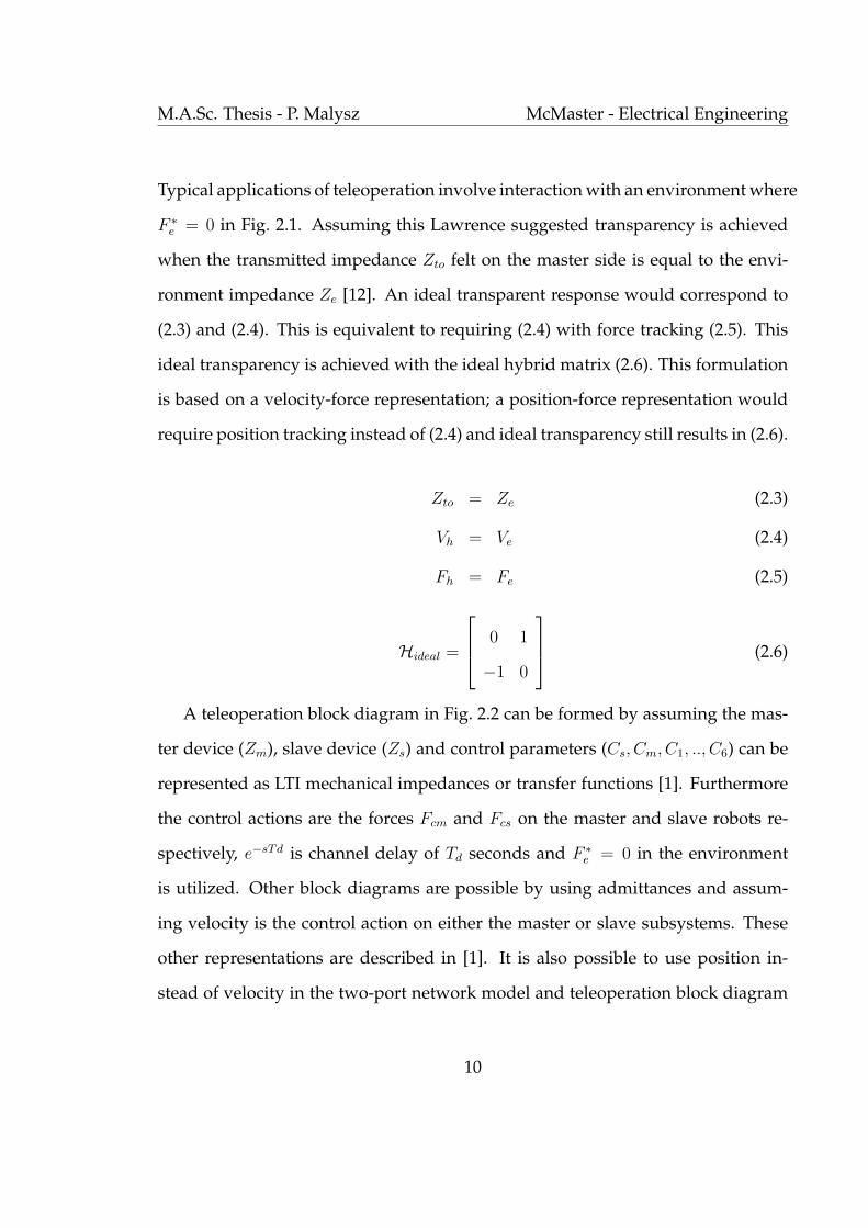
Typical applications of teleoperation involve interaction with an environment where
F ∗e = 0 in Fig. 2.1. Assuming this Lawrence suggested transparency is achieved
when the transmitted impedance Zto felt on the master side is equal to the envi-
ronment impedance Ze [12]. An ideal transparent response would correspond to
(2.3) and (2.4). This is equivalent to requiring (2.4) with force tracking (2.5). This
ideal transparency is achieved with the ideal hybrid matrix (2.6). This formulation
is based on a velocity-force representation; a position-force representation would
require position tracking instead of (2.4) and ideal transparency still results in (2.6).
Zto = Ze (2.3)
Vh = Ve (2.4)
Fh = Fe (2.5)
Hideal =
0 1
−1 0
(2.6)
A teleoperation block diagram in Fig. 2.2 can be formed by assuming the mas-
ter device (Zm), slave device (Zs) and control parameters (Cs, Cm, C1, .., C6) can be
represented as LTI mechanical impedances or transfer functions [1]. Furthermore
the control actions are the forces Fcm and Fcs on the master and slave robots re-
spectively, e−sTd is channel delay of Td seconds and F ∗e = 0 in the environment
is utilized. Other block diagrams are possible by using admittances and assum-
ing velocity is the control action on either the master or slave subsystems. These
other representations are described in [1]. It is also possible to use position in-
stead of velocity in the two-port network model and teleoperation block diagram
10

M.A.Sc. Thesis - P. Malysz McMaster - Electrical Engineering
by appropriately modifying the LTI impedances and transfer functions. An ad-
vantage of using velocity is that for mass-spring-damper mechanical systems a
velocity representation transforms directly to a capacitor-resistor-inductor electric
network. The linear systems discussed here can be realized through the applica-
tion of an appropriate linearizing controller on the non-linear robot dynamics.
Figure 2.2: Teleoperation block diagram. Figure from [1].
By choosing which channels to use for the control forces, the hybrid matrix
(2.1) can be found in terms of the control and dynamic parameters of the system.
The performance measures would be based on (2.1) and (2.2) where (2.3)-(2.6) is
desired. Teleoperation stability would reduce to closed-loop stability of Fig. 2.2
11

M.A.Sc. Thesis - P. Malysz McMaster - Electrical Engineering
2.1.2 Teleoperation Control Approaches
A literature search reveals many possible control architectures to facilitate teleop-
eration. Two-channel approaches can be obtained by only using two of the four
communication channels (C1, .., C4) shown in Fig. 2.2. A simple architecture that
requires no force sensing is position-position control [13], where in reference to
Fig. 2.2 C2 = C3 = C5 = C6 = 0 and position replaces velocity. Such an approach
can in effect couple the end-effectors of the master and slave robots with a vir-
tual spring-damper by using PD control where the master and slave controllers
have the same gains. Fidelity and transparency is poor especially in contact with
stiff environments and in the presence of communication time delays, however it is
simple to apply and has good robust stability. A velocity-velocity approach, where
master/slave velocities are matched, has an additional drawback of position drift
errors. To improve fidelity the use of force sensors can better reflect the mechanical
impedances in teleoperation. A force-force [14] architecture would only utilize the
two force measurements however it also suffers from position drift errors. When
only one force sensor is present a position-force [15] architecture can be used where
the force sensor should be placed on the slave robot. For superior transparency and
haptic fidelity all four communication channels should be utilized [12, 16]. Even
when using a multi-channel approach, ideal transparency still relies on accurate
acceleration measurement and good master/slave model knowledge to cancel out
the dynamics of the master/slave robots. Acceleration type measurements can be
obtained from force sensors and good model knowledge. However, sensitivity to
modeling errors can easily result in negative mass/damping and instability as a
result of eliminating the robot dynamics. Also, small zero-order-hold delays in
12

M.A.Sc. Thesis - P. Malysz McMaster - Electrical Engineering
discrete-time implementation can lead to instability.
Yokokohjii and Yoshikawa discuss transparency in terms of the teleoperation
system being able to act as a virtual tool between the operator and environment,
where an ideal tool would have no mass, stiffness or damping [16]. Even with ac-
celeration measurements a small amount of modeling error could give the virtual
tool negative mass [16], hence Yokokohjii and Yoshikawa propose the virtual tool
have some mechanical impedance to stabilize the system. Their transparency ob-
jectives are then generalized to (2.7) and position tracking (2.8) where mt, bt and kt
are the tool parameters.
Fh − Fe = mtx + btx + ktx (2.7)
xs = xm = x (2.8)
To achieve robust stability in the presence of dynamic uncertainty and com-
munication time delay, passivity based approaches can be utilized [17, 18]. These
approaches design controllers such that the two port network in Fig. 2.1 is a pas-
sive system. That is, the change in stored energy in the system over a given time
is less than the input energy to the system. A critical assumption to the approach
is passivity of the environment and user dynamics is required. This is because it
utilizes the fact that the interconnection of a passive 2-port network with passive
environment and user dynamics remain stable. One approach to show passivity of
the two-port network is to look at power rates and ensure the network stores en-
ergy at a rate equal to or less than the energy supply rate. The power input/output
rates can be obtained through the product of master/slave forces and velocities. A
drawback of these approaches is that the fidelity of haptic feedback can be greatly
13
M.A.Sc. Thesis - P. Malysz McMaster - Electrical Engineering
degraded.
For applications where the master and slave robots may be far apart, the issue
of time delay may be problematic since the time lags introduced can cause insta-
bility [19]. There exists extensive works on the time-delay problem, some of which
can be found in [18–20]. For more recent works one can refer to papers by Sirous-
pour and Shahdi [20–23]. In this thesis, time delay is assumed negligible since the
immediate applications in mind are ones where the entire teleoperation system is
in the same room.
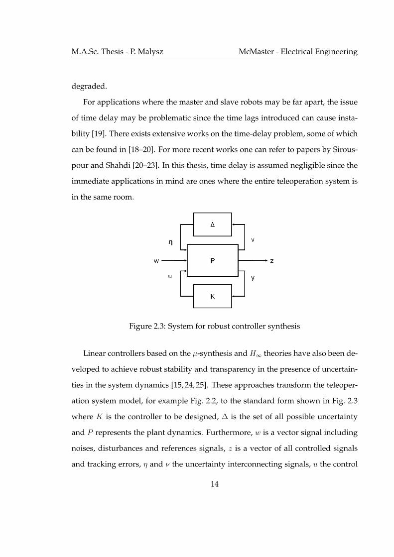
Figure 2.3: System for robust controller synthesis
Linear controllers based on the µ-synthesis and H∞ theories have also been de-
veloped to achieve robust stability and transparency in the presence of uncertain-
ties in the system dynamics [15, 24, 25]. These approaches transform the teleoper-
ation system model, for example Fig. 2.2, to the standard form shown in Fig. 2.3
where K is the controller to be designed, ∆ is the set of all possible uncertainty
and P represents the plant dynamics. Furthermore, w is a vector signal including
noises, disturbances and references signals, z is a vector of all controlled signals
and tracking errors, η and ν the uncertainty interconnecting signals, u the control
14
M.A.Sc. Thesis - P. Malysz McMaster - Electrical Engineering
signal and y the measurement. A fixed linear controller K is optimized such that
gain from w to z is small with the constraint of system stability. For stability the
small gain theorem is applied about the loop containing the uncertainty element
where it is assumed the H∞ norm of ∆ is bounded.
An adaptive/nonlinear controller is proposed in [26] which employs nonlinear
models of the master and slave robots to guarantee stability and transparency in
the presence of dynamic uncertainty. This adaptive approach is a teleoperation
extension of robotic adaptive control discussed by Slotine [27] and Sciavicco and
Siciliano [28] and can be used to linearize the teleoperation system. The method
is model-based since it requires models of both the master and slave systems to
be utilized in a feed-forward term in the control signal. The unknown parameters
of the master and slave systems are handled by adaptation. Convergence of the
tracking errors and adaptation errors is shown using Lyapunov stability theory.
This framework is used for the proposed controller in this thesis hence a detailed
explaination on this adaptive controller is given in the next chapter.
2.2 Telesurgery and Soft-tissue Telemanipulation
Increased interest in telerobotic-robotic surgery is being driven by applications in
minimally-invasive-robotic-surgery (MIRS) and robot assisted neurosurgery. MIRS
is intended to replace conventional minimally-invasive surgery (MIS), where hap-
tic fidelity is corrupted by surgical tool friction and non-intuitive motions pose
challenges in training and performing the surgery. For example, Perrault et al.
15
M.A.Sc. Thesis - P. Malysz McMaster - Electrical Engineering
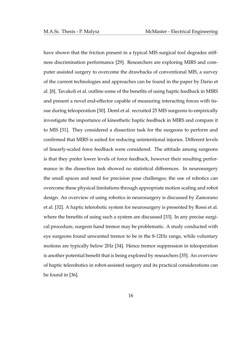
have shown that the friction present in a typical MIS surgical tool degrades stiff-
ness discrimination performance [29]. Researchers are exploring MIRS and com-
puter assisted surgery to overcome the drawbacks of conventional MIS, a survey
of the current technologies and approaches can be found in the paper by Dario et
al. [8]. Tavakoli et al. outline some of the benefits of using haptic feedback in MIRS
and present a novel end-effector capable of measuring interacting forces with tis-
sue during teleoperation [30]. Deml et al. recruited 25 MIS surgeons to empirically
investigate the importance of kinesthetic haptic feedback in MIRS and compare it
to MIS [31]. They considered a dissection task for the surgeons to perform and
confirmed that MIRS is suited for reducing unintentional injuries. Different levels
of linearly-scaled force feedback were considered. The attitude among surgeons
is that they prefer lower levels of force feedback, however their resulting perfor-
mance in the dissection task showed no statistical differences. In neurosurgery
the small spaces and need for precision pose challenges; the use of robotics can
overcome these physical limitations through appropriate motion scaling and robot
design. An overview of using robotics in neurosurgery is discussed by Zamorano
et al. [32]. A haptic telerobotic system for neurosurgery is presented by Rossi et al.
where the benefits of using such a system are discussed [33]. In any precise surgi-
cal procedure, surgeon hand tremor may be problematic. A study conducted with
eye surgeons found unwanted tremor to be in the 8-12Hz range, while voluntary
motions are typically below 2Hz [34]. Hence tremor suppression in teleoperation
is another potential benefit that is being explored by researchers [35]. An overview
of haptic telerobotics in robot-assisted surgery and its practical considerations can
be found in [36].
16

M.A.Sc. Thesis - P. Malysz McMaster - Electrical Engineering
In soft-tissue telemanipulation the design objectives must focus on the fidelity
of the system. Traditional measures of transparency involve position and force
tracking between master and slave such that the user would perceive the mechan-
ical impedance of the task environment without distortion [12]. Such an approach
could be restrictive particularly in fine tissue manipulation where human percep-
tion capabilities are limited. The work of Colgate in [24] is one of the early attempts
at altering the operator’s feel of the task through robust linear impedance shaping
using a hybrid two-port network framework. In his work the impedance is shaped
in the frequency domain where realistic shaping occurs only over a finite frequency
range.
More recently, optimization of task-based fidelity measures have been pro-
posed for soft-tissue telemanipulation assuming two-port hybrid network mod-
els [9, 10]. Cavusoglu et al. have proposed a fidelity measure that optimizes dif-
ferential environment impedance transmittance by explicitly formulating the goal
of optimization to maximize worst case differential fidelity [10]. In their work the
constraints of optimization were position tracking and stability where intervals
of expected hand and environment impedance were assumed. The environments
considered were those composed of spring and damper models where environ-
ment mass is neglected. De Gersem and Tendrick have also used an optimization
based approach to improve teleoperation fidelity [9]. Their goal in optimization is
to match transmitted impedance to scaled and mapped environment stiffness. The
environments considered are those only of soft spring models. The same tracking
and robust stability constraints were used in the optimization routine. The desired
17
M.A.Sc. Thesis - P. Malysz McMaster - Electrical Engineering
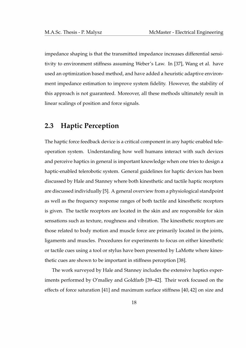
impedance shaping is that the transmitted impedance increases differential sensi-
tivity to environment stiffness assuming Weber’s Law. In [37], Wang et al. have
used an optimization based method, and have added a heuristic adaptive environ-
ment impedance estimation to improve system fidelity. However, the stability of
this approach is not guaranteed. Moreover, all these methods ultimately result in
linear scalings of position and force signals.
2.3 Haptic Perception
The haptic force feedback device is a critical component in any haptic enabled tele-
operation system. Understanding how well humans interact with such devices
and perceive haptics in general is important knowledge when one tries to design a
haptic-enabled telerobotic system. General guidelines for haptic devices has been
discussed by Hale and Stanney where both kinesthetic and tactile haptic receptors
are discussed individually [5]. A general overview from a physiological standpoint
as well as the frequency response ranges of both tactile and kinesthetic receptors
is given. The tactile receptors are located in the skin and are responsible for skin
sensations such as texture, roughness and vibration. The kinesthetic receptors are
those related to body motion and muscle force are primarily located in the joints,
ligaments and muscles. Procedures for experiments to focus on either kinesthetic
or tactile cues using a tool or stylus have been presented by LaMotte where kines-
thetic cues are shown to be important in stiffness perception [38].
The work surveyed by Hale and Stanney includes the extensive haptics exper-
iments performed by O’malley and Goldfarb [39–42]. Their work focused on the
effects of force saturation [41] and maximum surface stiffness [40, 42] on size and
18
M.A.Sc. Thesis - P. Malysz McMaster - Electrical Engineering
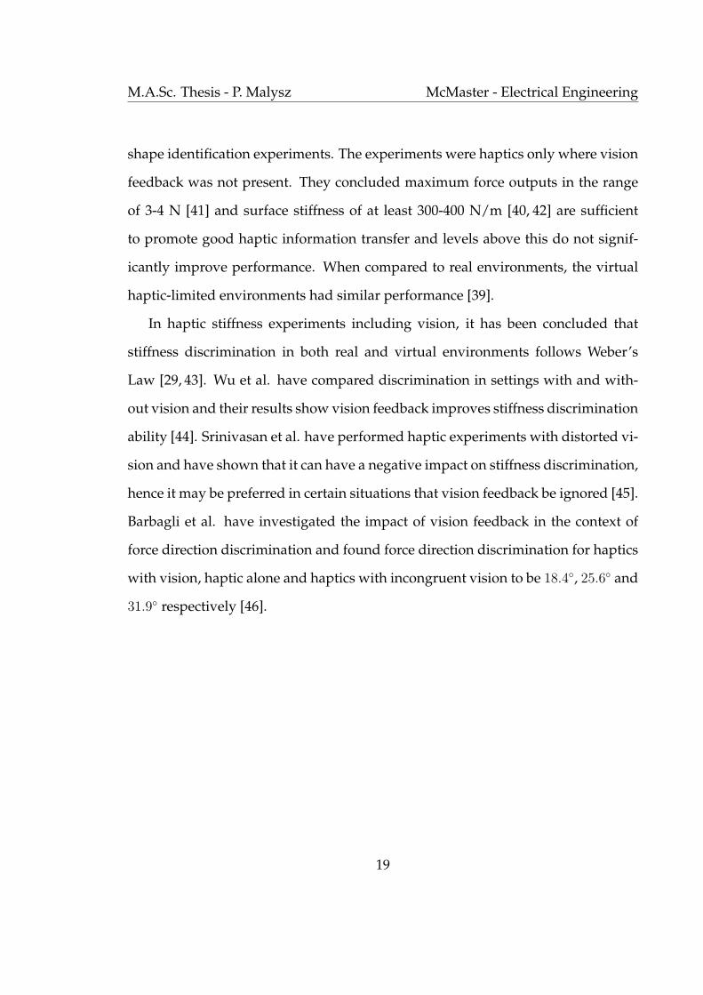
shape identification experiments. The experiments were haptics only where vision
feedback was not present. They concluded maximum force outputs in the range
of 3-4 N [41] and surface stiffness of at least 300-400 N/m [40, 42] are sufficient
to promote good haptic information transfer and levels above this do not signif-
icantly improve performance. When compared to real environments, the virtual
haptic-limited environments had similar performance [39].
In haptic stiffness experiments including vision, it has been concluded that
stiffness discrimination in both real and virtual environments follows Weber’s
Law [29, 43]. Wu et al. have compared discrimination in settings with and with-
out vision and their results show vision feedback improves stiffness discrimination
ability [44]. Srinivasan et al. have performed haptic experiments with distorted vi-
sion and have shown that it can have a negative impact on stiffness discrimination,
hence it may be preferred in certain situations that vision feedback be ignored [45].
Barbagli et al. have investigated the impact of vision feedback in the context of
force direction discrimination and found force direction discrimination for haptics
with vision, haptic alone and haptics with incongruent vision to be 18.4◦, 25.6◦ and
31.9◦ respectively [46].
19

Chapter 3
Lyapunov Based Adaptive Controllers
The dynamic models of the master and slave systems and their adaptive con-
trollers are presented in this chapter. These include models of the master/slave
robots as well as those of the hand and environment. A bilateral teleoperation
control scheme is proposed where position and force feedback measurements are
used locally and to facilitate teleoperation. Master/slave coordination is achieved
through bilateral communication of position and force information. The control
architecture is decentralized and the master and slave controllers employ an adap-
tive model-based component to allow convergence of tracking errors. Local stabil-
ity is proved using Lyapunov stability theory. The adaptive controllers are based
on those presented in [26] where they have been modified to accommodate the
desired generalized non-linear and filtered force/position mappings.
20
M.A.Sc. Thesis - P. Malysz McMaster - Electrical Engineering
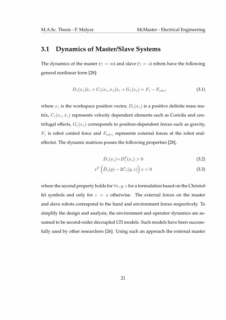
3.1 Dynamics of Master/Slave Systems
The dynamics of the master (γ = m) and slave (γ = s) robots have the following
general nonlinear form [28]:
Dγ(xγ)xγ + Cγ(xγ, xγ)xγ + Gγ(xγ) = Fγ − Fext,γ (3.1)
where xγ is the workspace position vector, Dγ(xγ) is a positive definite mass ma-
trix, Cγ(xγ, xγ) represents velocity dependent elements such as Coriolis and cen-
trifugal effects, Gγ(xγ) corresponds to position-dependent forces such as gravity,
Fγ is robot control force and Fext,γ represents external forces at the robot end-
effector. The dynamic matrices posses the following properties [28],
Dγ(xγ)=DTγ (xγ) > 0 (3.2)
xT(Dγ(y)− 2Cγ(y, z)
)x = 0 (3.3)
where the second property holds for ∀x, y, z for a formulation based on the Christof-
fel symbols and only for z = x otherwise. The external forces on the master
and slave robots correspond to the hand and environment forces respectively. To
simplify the design and analysis, the environment and operator dynamics are as-
sumed to be second-order decoupled LTI models. Such models have been success-
fully used by other researchers [26]. Using such an approach the external master
21

M.A.Sc. Thesis - P. Malysz McMaster - Electrical Engineering
robot forces are shown in (3.4) and for the slave robot in (3.5).
Fext,m = −Fh = − (F ∗h −Mhxm −Bhxm −Kh[xm − xm0]) (3.4)
Fext,s = Fe = Mexs + Bexs + Ke[xs − xs0] (3.5)
where Me, Mh, Be, Bh, Ke and Kh are positive diagonal matrices corresponding
to mass, damping and stiffness, xs0 and xm0 represent the contact points of the
environment and hand respectively, and F ∗h is the human exogenous input force
subject to (3.6) where ‖ · ‖∞ denotes the L∞ norm.
‖F ∗h‖∞ ≤ αh < +∞, αh > 0 (3.6)
Using (3.1), (3.5) and (3.4), the dynamics of the master and slave systems can
be represented by (3.7) and (3.8) respectively.
Mmxm + Cmxm + Gm = Fm + F ∗h (3.7)
Mm = Dm(xm) + Mh
Cm = Cm(xm, xm) + Bh
Gm = Gm(xm) + Kh[xm − xm0]
Msxs + Csxs + Gs = Fs (3.8)
Ms = Ds(xs) + Me
Cs = Cs(xs, xs) + Be
Gs = Gs(xs) + Ke[xs − xs0]
22

M.A.Sc. Thesis - P. Malysz McMaster - Electrical Engineering
To facilitate the teleoperation control design, the slave dynamics are rewritten in
mapped coordinates. By combining memoryless nonlinear monotonic mapping
κp(xs) and its derivative (3.10) with the slave dynamics in (3.8), one obtains (3.12)
qs = κp(xs) (3.9)
qs = κp(xs) = Jxs (3.10)
qs = κp(xs) = J xs + Jxs (3.11)
where J = ∂κ(.)∂xs
is a configuration-dependent Jacobian matrix.
MsJ−1Jxs + CsJ
−1qs + Gs = Fs (3.12)
By multiplying (3.12) by J−T and employing (3.11) the new slave dynamics shown
in (3.13) can be obtained.
M′sqs + C ′sqs + G ′s = J−T Fs (3.13)
M′s = J−TMsJ
−1
C ′s = J−T [Cs −MsJ−1J ]J−1
G ′s = J−TGs
The skew-symmetry property of Ms − 2Cs is preserved under the above nonlin-
ear coordinate transformation, i.e. M′s − 2C ′s is also skew-symmetric, as long as
J is nonsingular. This is seen by observing JTM′J − JTM′J in (3.14) is skew-
symmetric.
Ms − 2C = JTM′J − JTM′J + JT (M′s − 2C ′s)J (3.14)
23

M.A.Sc. Thesis - P. Malysz McMaster - Electrical Engineering
3.2 Control Design
The control design is divided into two subsections. The first subsection intro-
duces the local adaptive controllers assuming some desired command vectors. It
is shown that each local adaptive controller is stable via a suitable Lyapunov func-
tion. The second subsection gives the explicit form of the command vectors that
facilitate the generalized force/position mappings.
3.2.1 Local Adaptive Controllers
The combined dynamics of operator/master and slave/environment are nonlin-
ear and subject to uncertainty. Following a similar strategy to that in [26], local
adaptive control laws are introduced for the master and slave robots in (3.15) and
(3.16).
Fm = YmΘm +Kmρm − αhsign(ρm) (3.15)
Fs = JT [YsΘs +Ksρs] (3.16)
ρm = vmd −H ′xmvm + AHfhFh (3.17)
ρs = vsd −H ′xsκp(xs)− Aκf (HfeFe) (3.18)
H ′xm = 1 + Hxm, H ′
xs = 1 + Hxs (3.19)
where Hxm, Hxs, Hfe and Hfh are strictly proper stable LTI transfer functions, vmd
and vsd are master and slave command vectors to be introduced later, Km, Ks > 0,
24
M.A.Sc. Thesis - P. Malysz McMaster - Electrical Engineering
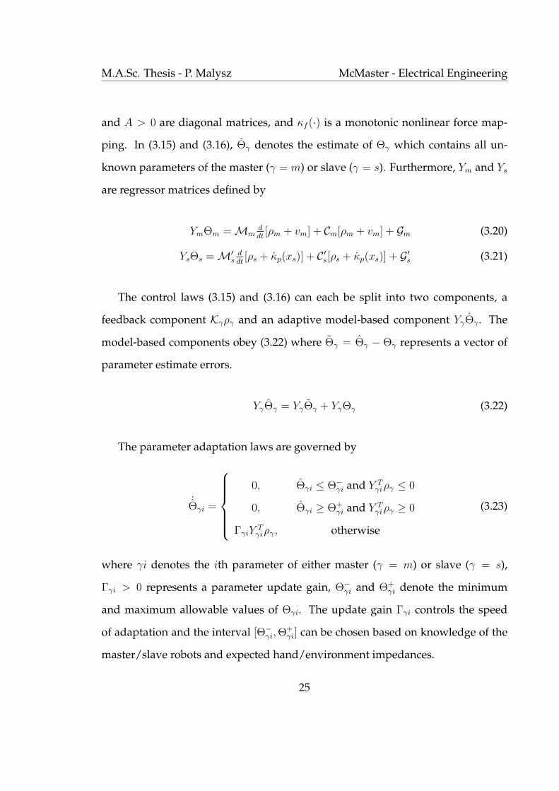
and A > 0 are diagonal matrices, and κf (·) is a monotonic nonlinear force map-
ping. In (3.15) and (3.16), Θγ denotes the estimate of Θγ which contains all un-
known parameters of the master (γ = m) or slave (γ = s). Furthermore, Ym and Ys
are regressor matrices defined by
YmΘm = Mmddt
[ρm + vm] + Cm[ρm + vm] + Gm (3.20)
YsΘs = M′s
ddt
[ρs + κp(xs)] + C ′s[ρs + κp(xs)] + G ′s (3.21)
The control laws (3.15) and (3.16) can each be split into two components, a
feedback component Kγργ and an adaptive model-based component YγΘγ . The
model-based components obey (3.22) where Θγ = Θγ − Θγ represents a vector of
parameter estimate errors.
YγΘγ = YγΘγ + YγΘγ (3.22)
The parameter adaptation laws are governed by
˙Θγi =
0, Θγi ≤ Θ−γi and Y T
γiργ ≤ 0
0, Θγi ≥ Θ+γi and Y T
γiργ ≥ 0
ΓγiYTγiργ, otherwise
(3.23)
where γi denotes the ith parameter of either master (γ = m) or slave (γ = s),
Γγi > 0 represents a parameter update gain, Θ−γi and Θ+
γi denote the minimum
and maximum allowable values of Θγi. The update gain Γγi controls the speed
of adaptation and the interval [Θ−γi, Θ
+γi] can be chosen based on knowledge of the
master/slave robots and expected hand/environment impedances.
25

M.A.Sc. Thesis - P. Malysz McMaster - Electrical Engineering
Combining master dynamics (3.7) with master control law (3.15) along with
(3.20) and (3.22) yields system dynamics (3.24) for the master subsystem.
−YmΘm = Mmρm + Cmρm +Kmρm + F ∗h − αhsign(ρm) (3.24)
The Lyapunov function (3.25) is chosen for master system dynamics (3.24).
Vm = 12ρT
mMmρm + 12ΘT
mΓ−1m Θm ≥ 0 (3.25)
where Γm is a constant diagonal matrix with diagonal elements equal to Γmi. Tak-
ing the derivative of Vm and using (3.24) yields
Vm = 12ρT
mMmρm + ρTm[−Cmρm−Kmρm−F ∗
h+αhsign(ρm)−YmΘm] + ˙ΘTmΓ−1
m Θm (3.26)
= 12ρT
m(Mm − 2Cm)ρm + ( ˙ΘTmΓ−1
m − ρTmYm)Θm − ρT
mKmρm + ρTmF ∗
h − ρTmαhsign(ρm)
Given the skew symmetry of Mm−2Cm, one finds 12ρT
m(Mm−2Cm)ρm = 0. Assum-
ing the true parameters Θm are constant, then ˙Θm =˙Θm and using (3.23) results in
( ˙ΘTmΓ−1
m − ρTmYm)Θm ≤ 0. Using (3.6) yields ρT
mF ∗h ≤ ρT
mαhsign(ρm). Therefore one
obtains
Vm ≤ −ρTmKmρm (3.27)
Since Vm ≤ 0, then Vm and ρm must have bounded maximum values meaning
ρm ∈ L∞. Taking the integral of (3.27) one can show∫∞0
ρTmKmρm dt < ∞, hence
ρm ∈ L2. Hence the signal belongs to L2 and L∞, i.e.
ρm ∈ L2 ∩ L∞ (3.28)
26

M.A.Sc. Thesis - P. Malysz McMaster - Electrical Engineering
Combining the mapped slave dynamics (3.13) with slave control law (3.16)
along with (3.21) and (3.22) yields the following slave system dynamics
−YsΘs = M′sρs + C ′sρs +Ksρs (3.29)
The following Lyapunov function is then defined
Vs = 12ρT
sM′sρs + 1
2ΘT
s Γ−1s Θs ≥ 0 (3.30)
where Γs is a constant diagonal matrix with diagonal elements equal to Γsi. Taking
the derivative of Vs and using (3.29) one can obtain
Vs = 12ρT
s (M′s − 2C ′s)ρs + ( ˙ΘT
s Γ−1s − ρT
s Ys)Θs − ρTsKsρs (3.31)
Since M′s − 2C ′s is also skew symmetric, assuming ˙Θs =
˙Θs and employing (3.23)
one obtains (3.32) and furthermore concludes (3.33).
Vs ≤ −ρTsKsρs (3.32)
ρs ∈ L2 ∩ L∞ (3.33)
27

M.A.Sc. Thesis - P. Malysz McMaster - Electrical Engineering
It should be noted that (3.20) and (3.21) contain the following
ρm + vm = vmd −Hxmvm + AHfhFh (3.34)
ρs + κp(xs) = vsd −Hxsκp(xs)− Aκf (HfeFe) (3.35)
Given the assumption on the strict properness of Hxm, Hfh, Hxs and Hfe , the terms
xm, Fh, κp(xs) and Fe would not be required when taking the derivatives of (3.34)
and (3.35). As will be seen in the next section, vmd and vsd would also be free of
these terms and therefore, acceleration and derivative of force are avoided in the
implementation of the master controller (3.15) and slave controller (3.16).
3.2.2 Teleoperation
The new master and slave control commands vmd and vsd in (3.17) and (3.18) must
be designed to achieve the stated objectives of teleoperation, i.e. establishing non-
linear and filtered force/position mappings between the operator and the environ-
ment. To this end let
vmd = H ′xs
˙κp(xs)− Aκf (HfeFe) + Λ[H ′xsκp(xs)−H ′
xmxm] (3.36)
vsd = H ′xmvm + AHfhFh + Λ[H ′
xmxm −H ′xsκp(xs)] (3.37)
where Λ > 0 is diagonal. If Q = xm, vm, κp(xs), κp(xs), then Q can be computed
from the following filter˙Q + CQ = CQ (3.38)
28

M.A.Sc. Thesis - P. Malysz McMaster - Electrical Engineering
It is worth noticing that the choice of the coordinating controllers in (3.36) and
(3.37) avoids acceleration and derivative of force measurements in vmd and vsd
which are needed in the local adaptive controllers.
Substituting (3.37) and (3.36) into (3.18) and (3.17) yield
ρm = [H ′xs
˙κp(xs)−H ′xmvm] + Λ[H ′
xsκp(xs)−H ′xmxm] + A[HfhFh−κf (HfeFe)] (3.39)
ρs = [H ′xmvm−H ′
xsκp(xs)] + Λ[H ′xmxm−H ′
xsκp(xs)] + A[HfhFh−κf (HfeFe)] (3.40)
Subtracting (3.40) and (3.39) gives
ρs − ρm = H ′xmvm −H ′
xs˙κp(xs) + Λ[H ′
xmxm −H ′xsκp(xs)] +
H ′xmvm −H ′
xsκp(xs) + Λ[H ′xmxm −H ′
xsκp(xs)] (3.41)
which can be rewritten as
X + X = ρs − ρm ∈ L2
⋂L∞ (3.42)
where
X = H ′xmvm −H ′
xsκp(xs) + Λ[H ′xmxm −H ′
xsκp(xs)] (3.43)
˙X + CX = CX (3.44)
The following result, Lemma 1 from [26], proves useful: Consider an equation
x + cx = u, where c > 0 is a positive constant and x is a differentiable function. If
u ∈ L∞, then x ∈ L∞ and x ∈ L∞; if u ∈ L2, then x ∈ L2 and x ∈ L2.
29
M.A.Sc. Thesis - P. Malysz McMaster - Electrical Engineering
Substituting (3.44) into (3.42) and using Lemma 1 from [26] yields ˙X ∈ L2
⋂L∞,
X ∈ L2
⋂L∞, and further
X ∈ L2
⋂L∞ (3.45)
Applying Lemma 1 from [26] again with (3.43) and (3.45) it follows that
ρe = H ′xmxm −H ′
xsκp(xs) ∈ L2 ∩ L∞ (3.46)
ρp = H ′xmvm −H ′
xsκp(xs) ∈ L2 ∩ L∞ (3.47)
This guarantees L2 and L∞ stability for both position and velocity tracking errors.
Adding (3.39) and (3.40) and exploiting−C−1 ˙Q = Q−Q from (3.38) one obtains
ρs+ρm = 2A[HfhFh−κf (HfeFe)]−C−1[H ′xm
˙vm+H ′xs
¨κp(xs)+ΛH ′xm
˙xm+ΛH ′xs
˙κp(xs)]
(3.48)
Using (3.46) and (3.47), Eq. (3.48) can be rewritten as
HfhFh − κf (HfeFe)− ρ = HZtxm (3.49)
with
ρ = 12A
[ρs + ρm − C−1(s + Λ)ρp] ∈ L2 ∩ L∞ (3.50)
HZt = H ′xm( C
s+C)Zt (3.51)
Zt = (AC)−1s2 + (AC)−1Λs (3.52)
The proposed generalized transparency objectives are expressed in (3.46) and
30
M.A.Sc. Thesis - P. Malysz McMaster - Electrical Engineering
(3.49). Nonlinear/filtered position tracking between master and slave is estab-
lished in (3.46) where the nonlinear mapping κp(·) and the LTI filters H ′xm and H ′
xs
can be chosen arbitrarily, subject to stability constraints that will be discussed in
later chapters. In the case of H ′xm = H ′
xs = 1 and κp(·) = κp, this would reduce to a
standard linear position scaling between master and slave. The nonlinear/filtered
force tracking between the user and environment, with an intervening virtual tool
dynamics, is demonstrated in (3.49). Again, the strictly proper LTI filters Hfh and
Hfe and the nonlinear mapping κf (·) can be arbitrarily selected subject to system
stability. The dynamics of the virtual tool perceived by the operator are given
by HZt/Hfh in (3.51) which are also adjustable by the control parameters. Un-
der quasi-static conditions, the user’s filtered hand force and nonlinearly mapped
filtered environment force would track each other. In the case of H ′xm = 1 and
Hfh ≈ 1, the tool behaves as a mass-damper link for frequencies below C rad/s.
If in addition κf (·) = κf and Hfe ≈ 1, a conventional scaled force tracking with
intervening mass-damper tool dynamics would result.
It must be noted that the stability of the local adaptive controllers, and the es-
tablishment of the generalized transparency objectives in (3.46) and (3.49) do not
guarantee the stability of the overall system and this must be analyzed separately.
The stability analysis can be simplified if the linear and nonlinear mappings are
decoupled along the different axes of motion and if the user and environment dy-
namics are also assumed decoupled in these axes. Under such circumstances, us-
ing the proposed local adaptive and teleoperation control laws, the overall closed-
loop dynamics are decoupled along the axes of motion. Therefore, without loss of
generality, only motion in one axis is considered.
31
M.A.Sc. Thesis - P. Malysz McMaster - Electrical Engineering
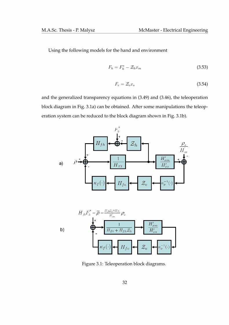
Using the following models for the hand and environment
Fh = F ∗h −Zhxm (3.53)
Fe = Zexs (3.54)
and the generalized transparency equations in (3.49) and (3.46), the teleoperation
block diagram in Fig. 3.1a) can be obtained. After some manipulations the teleop-
eration system can be reduced to the block diagram shown in Fig. 3.1b).
Figure 3.1: Teleoperation block diagrams.
32
M.A.Sc. Thesis - P. Malysz McMaster - Electrical Engineering
It should be noted that the user and environment impedances Zh and Ze in
Fig. 3.1 are usually unknown and subject to parametric uncertainty. Assuming
κp(·), κf (·) are linear, H ′xm = H ′
xs = 1 and Hfe = Hfh = Cs+C
leads to the guaranteed
stability result obtained in [26], i.e.
ρm, ρs, ρe, ρp, ρ → 0 (3.55)
vm, vs ∈ L∞ (3.56)
This stability result is valid for all mass-damper-spring type user and environ-
ment dynamics. In the general case of nonlinear and filtered force/position map-
pings, new conditions for robust stability must be derived. This will be discussed
in later chapters. Specifically, interval plant systems theory presented in Chap-
ter 4 and non-linear stability of Lur’e-Postnikov systems discussed in Chapter 5
are utilized and a stability analysis is shown in Chapter 6.
33

Chapter 4
Interval Plant Systems
Interval plant systems are families of plants that are parameterized by a set of in-
tervals. Such systems are useful since a standard approach to show robust stability
of a control system is to assume the plant transfer function is an interval plant sys-
tem. Typically the coefficients of the transfer function polynomials are assumed
to be some function of the interval parameters. In this chapter two special classes
of interval plant systems are considered, Kharitonov plants and polytopic plants.
In both cases it is assumed that the transfer functions for these plants have nu-
merator and denominator polynomials whose parameters are independent of each
other. The rest of this chapter will discuss some properties of these polynomials
and present methods for finding the Bode and Nyquist envelopes of both plant
systems. These methods are useful since they are used to show robust stability of
the teleoperation block diagram in Fig. 3.1.
34

M.A.Sc. Thesis - P. Malysz McMaster - Electrical Engineering
4.1 Interval Polynomials
Two special classes of interval polynomials are presented in this section. The first
being polynomials with real independent interval coefficients, they are best ana-
lyzed using Kharitonov polynomials. The second are polynomials with real lin-
early dependent coefficients, referred to as polytopic polynomials.
4.1.1 Kharitonov Polynomials
Kharitonov polynomials are typically used to describe parametric polynomials of
the following form
F(s) = δ0 + δ1s + δ2s2 + δ3s
3 + .... (4.1)
δ−i ≤ δi ≤ δ+i
where δi are real, independent of each other and lie in the interval [δ−i , δ+i ]. Sub-
stituting s = jω into (4.1) and splitting it into its odd (imaginary) and even (real)
parts yield
Feven(ω) = δ0 − δ2ω2 + δ4ω
6 − δ6ω8 + .... (4.2)
Fodd(ω)
jω= δ1 − δ3ω
2 + δ5ω6 − δ7ω
8 + .... (4.3)
35
M.A.Sc. Thesis - P. Malysz McMaster - Electrical Engineering
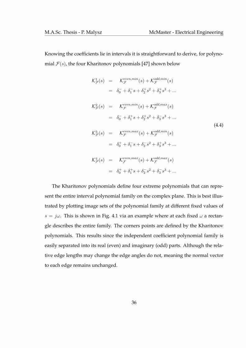
Knowing the coefficients lie in intervals it is straightforward to derive, for polyno-
mial F(s), the four Kharitonov polynomials [47] shown below
K1F(s) = Keven,min
F (s) +Kodd,minF (s)
= δ−0 + δ−1 s + δ+2 s2 + δ+
3 s3 + ...
K2F(s) = Keven,min
F (s) +Kodd,maxF (s)
= δ−0 + δ+1 s + δ+
2 s2 + δ−3 s3 + ...
K3F(s) = Keven,max
F (s) +Kodd,minF (s)
= δ+0 + δ−1 s + δ−2 s2 + δ+
3 s3 + ...
K4F(s) = Keven,max
F (s) +Kodd,maxF (s)
= δ+0 + δ+
1 s + δ−2 s2 + δ−3 s3 + ...
(4.4)
The Kharitonov polynomials define four extreme polynomials that can repre-
sent the entire interval polynomial family on the complex plane. This is best illus-
trated by plotting image sets of the polynomial family at different fixed values of
s = jω. This is shown in Fig. 4.1 via an example where at each fixed ω a rectan-
gle describes the entire family. The corners points are defined by the Kharitonov
polynomials. This results since the independent coefficient polynomial family is
easily separated into its real (even) and imaginary (odd) parts. Although the rela-
tive edge lengths may change the edge angles do not, meaning the normal vector
to each edge remains unchanged.
36

M.A.Sc. Thesis - P. Malysz McMaster - Electrical Engineering
−14000 −12000 −10000 −8000 −6000 −4000 −2000 0 20000
2000
4000
6000
8000
10000
12000
14000
Real
Imag
inar
y
Figure 4.1: Image sets of Ze = δ2s2 + δ1s + δ0 from ω = 63 rad/s to 251 rad/s.
Interval ranges: δ2 ∈ [0.01, 0.2], δ1 ∈ [5, 50] and δ2 ∈ [10, 1000]
Given the mentioned properties of Kharitonov polynomials, it is simple to de-
rive a Hurwitz stability condition for real independent coefficient polynomial fam-
ily. Assuming at least one member of the interval polynomial family is Hurwitz
stable, i.e. one of the Kharitonov polynomials is Hurwitz, then the entire polyno-
mial family is Hurwitz stable if and only if all four Kharitonov polynomials are
Hurwitz [48].
Using the rectangular image set interpretation of the interval polynomial fam-
ily, Hurwitz stability results if the origin is excluded from every rectangular image
set at all frequencies of ω. Given that the roots of the polynomials change con-
tinuously and there exists at least one stable member, origin exclusion implies no
37

M.A.Sc. Thesis - P. Malysz McMaster - Electrical Engineering
marginally stable roots on the jω axis for the entire polynomial family. Origin
exclusion of the image set can be shown to be equivalent to the four Kharitonov
polynomials being Hurwitz stable [48]. One approach to show this is to use the
contradiction argument given in section 5.4.2 of [48], where it is shown that in the
limiting case the origin is on an edge entering the rectangle the monotonic phase
property of one of the Hurwitz Kharitonov polynomials would be violated.
4.1.2 Polytopic Polynomials
Polynomials with real linearly dependent interval coefficients of the form (6.15)
are considered to be polytopic polynomials.
C(s) = a0(q) + a1(q)s + ... + an(q)sn (4.5)
q = [δ0, δ1, ..., δn]T (4.6)
δ−i ≤ δi ≤ δ+i
The multidimensional variable q represents a (convex) hyper-rectangular uncer-
tainty space and ai(q) a real polynomial coefficient that depends linearly/affinely
on the elements of q. Linearly dependent interval coefficient polynomials have
the polytopic property such that the image sets of C(s) at fixed s = jw define a
bounded polytope or convex polygon [49] [2]. This is illustrated via an example
in Fig. 4.2, where it is seen each image set is a convex polygon which can change
shape and rotate and represents a different frequency ranging from 5 rad/s to 70
rad/s. Interval ranges: δ5 ∈ [0.4, 0.7], δ4 ∈ [0.01, 0.2], δ3 ∈ [15, 115], δ2 ∈ [5, 50],
δ1 ∈ [20, 1000], and δ0 ∈ [10, 1000]. A convex polygon is expected since linear/affine
38
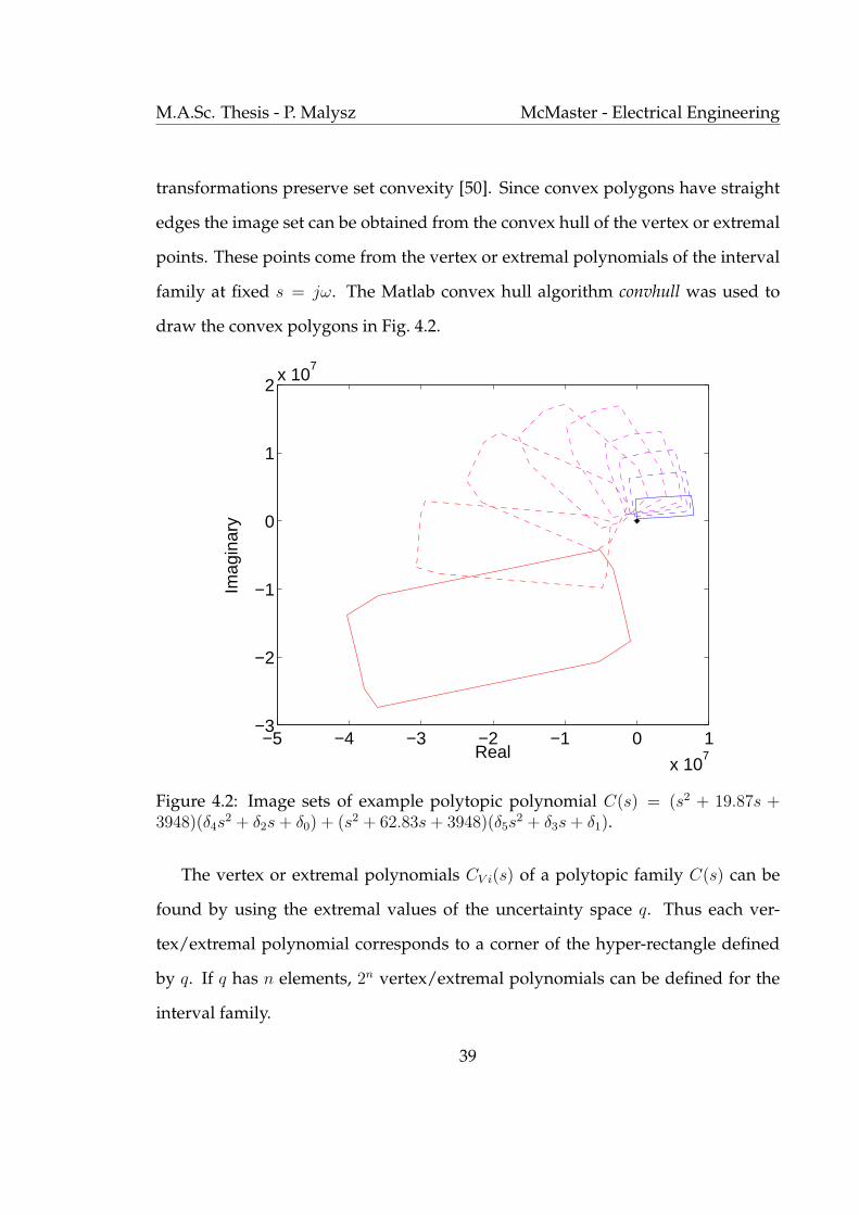
M.A.Sc. Thesis - P. Malysz McMaster - Electrical Engineering
transformations preserve set convexity [50]. Since convex polygons have straight
edges the image set can be obtained from the convex hull of the vertex or extremal
points. These points come from the vertex or extremal polynomials of the interval
family at fixed s = jω. The Matlab convex hull algorithm convhull was used to
draw the convex polygons in Fig. 4.2.
−5 −4 −3 −2 −1 0 1
x 107
−3
−2
−1
0
1
2x 10
7
Real
Imag
inar
y
Figure 4.2: Image sets of example polytopic polynomial C(s) = (s2 + 19.87s +3948)(δ4s
2 + δ2s + δ0) + (s2 + 62.83s + 3948)(δ5s2 + δ3s + δ1).
The vertex or extremal polynomials CV i(s) of a polytopic family C(s) can be
found by using the extremal values of the uncertainty space q. Thus each ver-
tex/extremal polynomial corresponds to a corner of the hyper-rectangle defined
by q. If q has n elements, 2n vertex/extremal polynomials can be defined for the
interval family.
39

M.A.Sc. Thesis - P. Malysz McMaster - Electrical Engineering
When dealing with polytopic polynomials one is typically interested in apply-
ing the Edge theorem [51] [48], where the edges of the hyper-rectangular param-
eter space q are checked. In particular a subset of these edges define the convex
polygon image sets previously discussed. For a q of dimension n with 2n ver-
tices, 2n−1(2n − 1) interconnecting edges can be defined. These interconnecting
edges connect all vertices to each other. The number of edges to be checked can
be reduced to 2n−1n by using only the outer exposed edges of the hyper-rectangle
q [48]. An exposed edge is defined as being able to move from one vertex to an-
other by only varying one dimension. This concept of varying along a dimen-
sion can be utilized to derive the exposed edge formula with the aid of Fig. 4.3
where Nee(n) denotes the number of exposed edges of an object with dimension
n. It is seen the number of exposed edges follows a recursive pattern given by
Nee(n) = 2Nee(n− 1) + 2n−1, solving this yields Nee(n) = 2n−1n.
Figure 4.3: Number of exposed edges as a function of object dimension a) pointNee(0) = 0 b) line Nee(1) = 1 c) square Nee(2) = 4 d) cube Nee(3) = 12 e) tasseract(4-D hypercube) Nee(4) = 32
40

M.A.Sc. Thesis - P. Malysz McMaster - Electrical Engineering
The edges of the convex polygon image set at fixed s = jω come from a subset
of the outer exposed edges. In particular the polygon is composed of at most 2n
edges and 2n vertices assuming q has dimension n [2]. The explanation of this is
given as follows. The 2n−1n exposed edges can be divided into n groups where
in each group 2n−1 edges are parallel to each other when mapped to the complex
plane image set. The mapped exposed edges in each group that, when extended,
have the minimum and maximum intersections with the imaginary (or real) axis
are the ones that compose two edges of the convex polygon. This is shown in
Fig. 4.4 where the uncertainty space has dimension three.
Figure 4.4: Image sets with uncertainty dimension n = 3 a) image of mappedexposed edges b) 2-n convex polygon. Figure modified from [2].
This reduction in the number of vertices and edges can greatly improve the
computation efficiency of algorithms that utilize vertex and edge checking. It
should be noted that this reduced set of vertices/edges may change as the variable
s = jω is varied, hence identifying the 2n edges/vertices is a non-trival matter.
One approach is to use a convex hull finding algorithm, such as Matlab convhull,
at each s = jω to find this reduced set of vertices/edges.
41

M.A.Sc. Thesis - P. Malysz McMaster - Electrical Engineering
Vertex and edge checking is desired when one would like to show an inter-
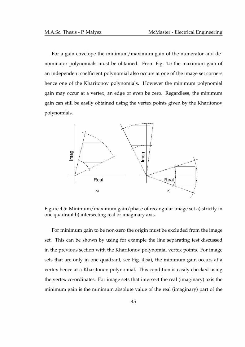
val polytopic polynomial family of the form (6.15) is Hurwitz stable. As with the
Kharitonov polynomial image sets, Hurwitz stability of the polytopic polynomial
family is assured if and only if the origin is excluded from the 2n convex poly-
gon image sets at every frequency ω. In contrast with Kharitonov polynomials
Hurwitz stability of the vertex/extremal polynomials does not guarantee stability
of the whole interval family [48]. Fortunately the polytopic property of the im-
age sets still allows for a vertex only stability check that avoids computationally
expensive edge checking [49].
A convex polygon can be shown to exclude the origin if and only if a line can
be found that separates the vertices of the polygon from the origin. If such a line
can be found at every frequency Hurwitz stablity follows since no marginally sta-
ble roots exist. The implementation of such a test may require an extra sweeping
variable to find such a separating line, an idea central to the approach outlined
in [49]. Since only Hurwitz stability is being considering the need for this line
slope sweeping variable is avoided by utilizing the phase of the vertex/extremal
polynomials of the polytopic polynomial family. For ease in implementation an
offset phase value for each vertex polynomial has been developed as follows
φCV i(ω) = Arg(CV i(jω))−Arg(CV ∗(jω)) + 2πk (4.7)
where CV i(s) is a vertex polynomial, CV ∗ an arbitrary vertex polynomial, Arg(·)returns the principal argument of a complex number and an integer value of k is
42

M.A.Sc. Thesis - P. Malysz McMaster - Electrical Engineering
chosen as
k =
−1, Arg(CV i(jω))−Arg(CV ∗(jω)) > π
1, Arg(CV i(jω))−Arg(CV ∗(jω)) < −π
0, otherwise
(4.8)
so that (4.9) is satisfied.
−π ≤ φCV i(ω) ≤ π (4.9)
Note the arbitrary vertex polynomial CV ∗ need not be the same for all frequencies
but must be the same for all φCV i(ω) for a given fixed ω.
This phase offset transformation has the effect of rotating the convex hulls at
each frequency so that they all intersect the positive real axis. The origin is ex-
cluded from the image sets of C(jω) if and only if the maximum phase difference
among φCV i(ω) at every frequency ω is less than π. The proof of this is obvious
using plane geometry. The stability condition can thus be written as (4.10).
supω∈<+
[maxi
φCV i(ω)−min
iφCV i
(ω)] < π (4.10)
The implementation of (4.10) in a stability analysis is simple since it only requires
phase values between −π and π of a limited set of known vertex polynomials.
43

M.A.Sc. Thesis - P. Malysz McMaster - Electrical Engineering
4.2 Kharitonov Plants
Interval plant systems where the numerator and denominator polynomials are
real independent coefficient polynomials are suited to be analyzed by Kharitonov
plants. For a transfer function T (s) = N (s)D(s)
with independent interval coefficients,
sixteen Kharitonov plants can be defined as follows
TK(s) =
{KiN (s)
KkD(s)
: i, k ∈ {1, 2, 3, 4}}
(4.11)
where the Kharitonov polynomials have been defined in (4.4). The rest of this
section will describe methods of constructing Bode and Nyquist envelopes of in-
dependent coefficient interval plant systems.
4.2.1 Bode Envelope
A Bode envelope for an independent coefficient interval plant tranfer function
T (s) = N (s)D(s)
can be constructed with the aid of Kharitonov plants (4.11) and Khari-
tonov polynomials (4.4). The minimum/maximum phase of T (jω) can be found
from the minimum/maximum phase of the sixteen Kharitonov plants TK(jω) [48].
This follows since at a given frequency ω the extreme phase values of both numer-
ator and denominator polynomials of T (jω) occur at one of its Kharitonov polyno-
mials via the rectangular image set argument. This is illustrated is Fig. 4.5. For the
case where the origin may potentially go through the image set phase continuity of
the Kharitonov polynomials is used to show the phase envelope still results from
the Kharitonov polynomials.
44
M.A.Sc. Thesis - P. Malysz McMaster - Electrical Engineering
For a gain envelope the minimum/maximum gain of the numerator and de-
nominator polynomials must be obtained. From Fig. 4.5 the maximum gain of
an independent coefficient polynomial also occurs at one of the image set corners
hence one of the Kharitonov polynomials. However the minimum polynomial
gain may occur at a vertex, an edge or even be zero. Regardless, the minimum
gain can still be easily obtained using the vertex points given by the Kharitonov
polynomials.
Figure 4.5: Minimum/maximum gain/phase of recangular image set a) strictly inone quadrant b) intersecting real or imaginary axis.
For minimum gain to be non-zero the origin must be excluded from the image
set. This can be shown by using for example the line separating test discussed
in the previous section with the Kharitonov polynomial vertex points. For image
sets that are only in one quadrant, see Fig. 4.5a), the minimum gain occurs at a
vertex hence at a Kharitonov polynomial. This condition is easily checked using
the vertex co-ordinates. For image sets that intersect the real (imaginary) axis the
minimum gain is the minimum absolute value of the real (imaginary) part of the
45
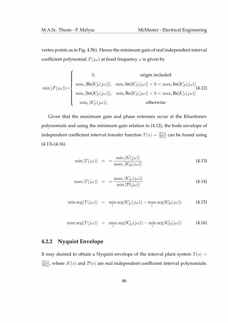
M.A.Sc. Thesis - P. Malysz McMaster - Electrical Engineering
vertex points as in Fig. 4.5b). Hence the minimum gain of real independent interval
coefficient polynomial F(jω) at fixed frequency ω is given by
min |F(jω)|=
0, origin included
mini |Re[KiF(jω)]|, mini Im[Ki
F(jω)] < 0 < maxi Im[KiF(jω)]
mini |Im[KiF(jω)]|, mini Re[Ki
F(jω)] < 0 < maxi Re[KiF(jω)]
mini |KiF(jω)|, otherwise
(4.12)
Given that the maximum gain and phase extremes occur at the Kharitonov
polynomials and using the minimum gain relation in (4.12), the bode envelope of
independent coefficient interval transfer function T (s) = N (s)D(s)
can be found using
(4.13)-(4.16).
min |T (jω)| = =min |N (jω)|
maxi |KiD(jω)| (4.13)
max |T (jω)| = =maxi |Ki
N (jω)|min |D(jω)| (4.14)
min arg(T (jω)) = mini
arg(KiN (jω))−max
iarg(Ki
D(jω)) (4.15)
max arg(T (jω)) = maxi
arg(KiN (jω))−min
iarg(Ki
D(jω)) (4.16)
4.2.2 Nyquist Envelope
It may desired to obtain a Nyquist envelope of the interval plant system T (s) =
N (s)D(s)
, where N (s) and D(s) are real independent coefficient interval polynomials.
46
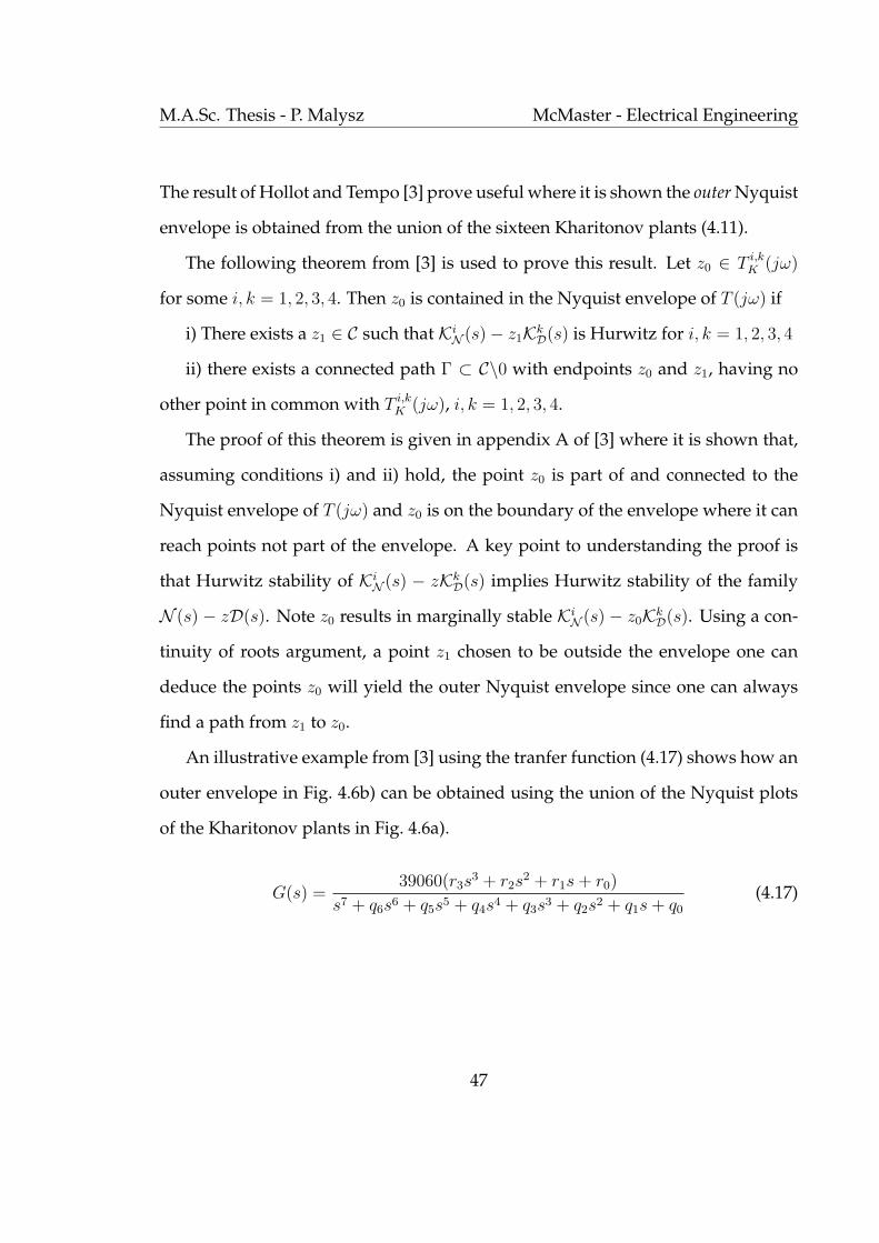
M.A.Sc. Thesis - P. Malysz McMaster - Electrical Engineering
The result of Hollot and Tempo [3] prove useful where it is shown the outer Nyquist
envelope is obtained from the union of the sixteen Kharitonov plants (4.11).
The following theorem from [3] is used to prove this result. Let z0 ∈ T i,kK (jω)
for some i, k = 1, 2, 3, 4. Then z0 is contained in the Nyquist envelope of T (jω) if
i) There exists a z1 ∈ C such that KiN (s)− z1Kk
D(s) is Hurwitz for i, k = 1, 2, 3, 4
ii) there exists a connected path Γ ⊂ C\0 with endpoints z0 and z1, having no
other point in common with T i,kK (jω), i, k = 1, 2, 3, 4.
The proof of this theorem is given in appendix A of [3] where it is shown that,
assuming conditions i) and ii) hold, the point z0 is part of and connected to the
Nyquist envelope of T (jω) and z0 is on the boundary of the envelope where it can
reach points not part of the envelope. A key point to understanding the proof is
that Hurwitz stability of KiN (s) − zKk
D(s) implies Hurwitz stability of the family
N (s) − zD(s). Note z0 results in marginally stable KiN (s) − z0Kk
D(s). Using a con-
tinuity of roots argument, a point z1 chosen to be outside the envelope one can
deduce the points z0 will yield the outer Nyquist envelope since one can always
find a path from z1 to z0.
An illustrative example from [3] using the tranfer function (4.17) shows how an
outer envelope in Fig. 4.6b) can be obtained using the union of the Nyquist plots
of the Kharitonov plants in Fig. 4.6a).
G(s) =39060(r3s
3 + r2s2 + r1s + r0)
s7 + q6s6 + q5s5 + q4s4 + q3s3 + q2s2 + q1s + q0
(4.17)
47
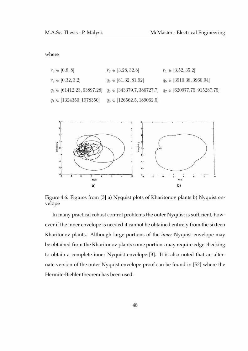
M.A.Sc. Thesis - P. Malysz McMaster - Electrical Engineering
where
r3 ∈ [0.8, 8] r2 ∈ [3.28, 32.8] r1 ∈ [3.52, 35.2]
r2 ∈ [0.32, 3.2] q6 ∈ [81.32, 81.92] q5 ∈ [3910.38, 3960.94]
q4 ∈ [61412.23, 63897.28] q3 ∈ [343379.7, 386727.7] q2 ∈ [620977.75, 915287.75]
q1 ∈ [1324350, 1978350] q0 ∈ [126562.5, 189062.5]
Figure 4.6: Figures from [3] a) Nyquist plots of Kharitonov plants b) Nyquist en-velope
In many practical robust control problems the outer Nyquist is sufficient, how-
ever if the inner envelope is needed it cannot be obtained entirely from the sixteen
Kharitonov plants. Although large portions of the inner Nyquist envelope may
be obtained from the Kharitonov plants some portions may require edge checking
to obtain a complete inner Nyquist envelope [3]. It is also noted that an alter-
nate version of the outer Nyquist envelope proof can be found in [52] where the
Hermite-Biehler theorem has been used.
48
M.A.Sc. Thesis - P. Malysz McMaster - Electrical Engineering
4.3 Polytopic Plants
Assuming an interval plant transfer function contains polynomials with linearly
dependent coefficients is far less restrictive than an independent coefficient ap-
proach suited for Kharitonov polynomials. This section presents methods for ob-
taining Bode and Nyquist envelopes for polytopic plants of the form (4.18) whose
numerator and denominator polynomials are polytopic polynomials whose inter-
val parameters are independent of each other. The methods described here are
those that are found in [2].
P (s) =N(s)
D(s)=
a0(q) + a1(q)s + ... + an(q)sn
b0(r) + b1(r)s + ... + bm(r)sm(4.18)
q = [δ0, δ1, ..., δn]T , r = [ϑ0, ϑ1, ..., ϑm]T
δ−i ≤ δi ≤ δ+i , ϑ−i ≤ ϑi ≤ ϑ+
i
4.3.1 Bode Envelope
Since it is assumed the numerator and denominator polynomials are independent
of each other, the Bode envelope of polytopic plant P (s) is found by finding the
phase and gain envelopes of N(jω) and D(jω).
As was stated before, polytopic polynomials have image sets that are convex
polygons whose vertices from a subset of the vertex polynomials. Like rectangular
image sets, convex polygon image sets have their extreme phase values and maxi-
mum gain at the vertices, e.g. see Fig. 4.7. Minimum gain can potentially occur at
49

M.A.Sc. Thesis - P. Malysz McMaster - Electrical Engineering
an edge or be zero. To test for zero gain the origin exclusion ideas discussed be-
fore can be applied. To handle minimum gain potentially occurring on an edge the
methods described in [2] are utilized to find minimum gain using only the vertices.
Figure 4.7: Minimum/maximum gain/phase of convex polygon image set
The minimum gain of polytopic polynomials C(s) at fixed s = jω assuming
non-zero minimum gain is given by (4.19) [2]
min |C(jω)| =
|vi|, |vi| < |k1| and |vi| < |k2|l1 |k1| < |vi| and |k2| >= |vi|l2 |k2| < |vi| and |k1| >= |vi|
min(l1, l2) |k1| < |vi| and |k2| < |vi|
(4.19)
where vi is the vertex closest to the origin and v1 and v2 are edge adjacent vertices
as shown in Fig. 4.8. Points k1 and k2 are close to vi specified by equation (4.20)
where λ is a small number typically about 10−6. Scalars l1 and l2 are distances from
50

M.A.Sc. Thesis - P. Malysz McMaster - Electrical Engineering
the line equations defined by the edges adjacent to vi whose exact values are given
by (4.21) and (4.22).
k1,2 = vi(1− λ) + λv1,2 (4.20)
l1,2 =
√(2|vi|ρ1,2)2 − (|vi|2 − |v1,2|2 + ρ2
1,2)2
2ρ1,2
(4.21)
ρ1,2 =√
(Re[v1,2]− Re[vi])2 + (Im[v1,2]− Im[vi])2 (4.22)
Figure 4.8: Minimum gain of convex polygon image set.
51
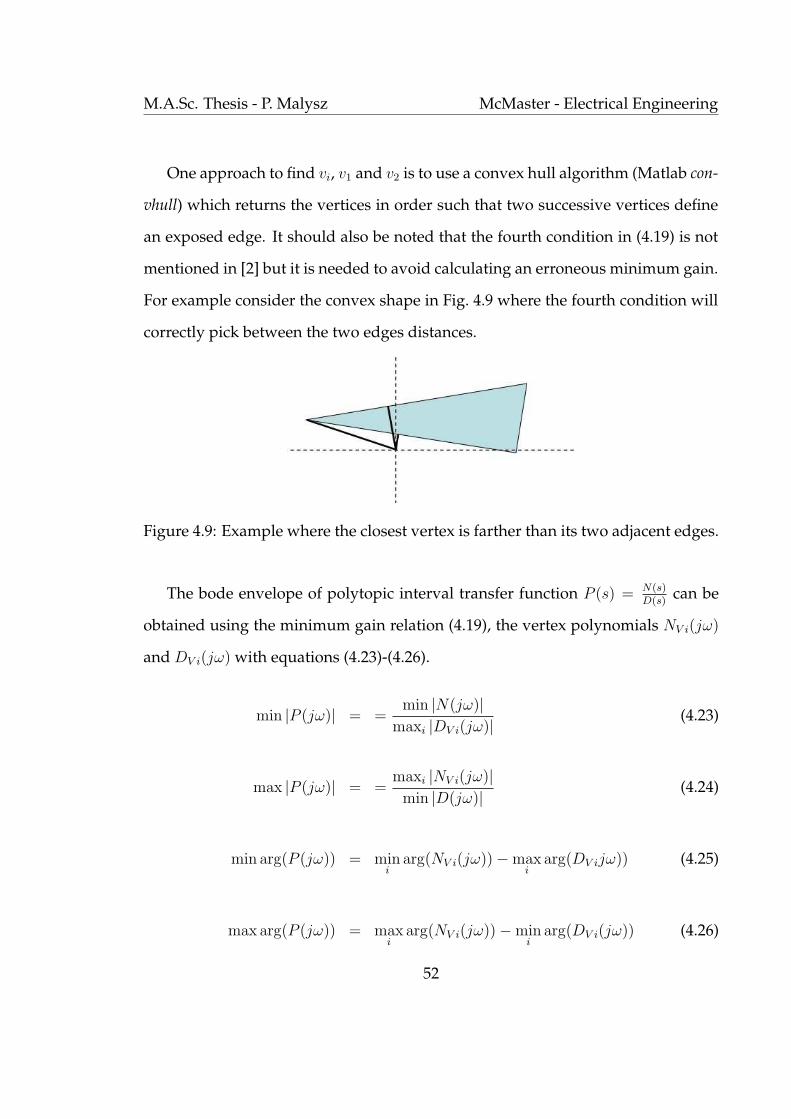
M.A.Sc. Thesis - P. Malysz McMaster - Electrical Engineering
One approach to find vi, v1 and v2 is to use a convex hull algorithm (Matlab con-
vhull) which returns the vertices in order such that two successive vertices define
an exposed edge. It should also be noted that the fourth condition in (4.19) is not
mentioned in [2] but it is needed to avoid calculating an erroneous minimum gain.
For example consider the convex shape in Fig. 4.9 where the fourth condition will
correctly pick between the two edges distances.
Figure 4.9: Example where the closest vertex is farther than its two adjacent edges.
The bode envelope of polytopic interval transfer function P (s) = N(s)D(s)
can be
obtained using the minimum gain relation (4.19), the vertex polynomials NV i(jω)
and DV i(jω) with equations (4.23)-(4.26).
min |P (jω)| = =min |N(jω)|
maxi |DV i(jω)| (4.23)
max |P (jω)| = =maxi |NV i(jω)|min |D(jω)| (4.24)
min arg(P (jω)) = mini
arg(NV i(jω))−maxi
arg(DV ijω)) (4.25)
max arg(P (jω)) = maxi
arg(NV i(jω))−mini
arg(DV i(jω)) (4.26)
52
M.A.Sc. Thesis - P. Malysz McMaster - Electrical Engineering
4.3.2 Nyquist Envelope
The Nyquist envelope of polytopic plants of the form (4.18) cannot, in general,
be formed from the union of special extremal plants [2] [48]. An application of
the Edge theorem [51] is necessary to determine the Nyquist envelope of (4.18).
Specifically the method described in [2] is used where the exposed edges/vertices
of the convex polygon image sets of N(jω) and D(jω) are utilized as minimal sets
of vertices and edges to be used in forming the required Nyquist envelope. This
approach reduces the number of edges from 2n−1n uncertainty box outer exposed
edges to 2n and reduces the number of vertices from 2n to 2n; here n represents the
number of unknown interval parameters in polynomial N(s) or D(s) [2].
To identify the reduced set of vertices and edges a convex hull algorithm, such
as Matlab convhull, can be utilized with the vertex points given by vertex polyno-
mials NV i(jω) and DV i(jω) at fixed frequency ω. The convex hull algorithm should
return the convex hull vertices in an order such that two successive vertices define
an exposed edge of the convex polygon image set of N(jω) or D(jω). Once this re-
duced set of vertices and edges have been identified the boundary of the Nyquist
envelope of P (jω) at fixed ω is given by [2]
δP (jω) ⊂ SNV
SDE
∪ SNE
SDV
(4.27)
SNV= {vN
1 , vN2 , ..., vN
p } (4.28)
SNE= {(1− λ)vN
1 + λvN2 , (1− λ)vN
2 + λvN3 ,
..., (1− λ)vNp + λvN
1 }, λ ∈ [0, 1] (4.29)
53

M.A.Sc. Thesis - P. Malysz McMaster - Electrical Engineering
SDV= {vD
1 , vD2 , ..., vD
r } (4.30)
SDE= {(1− λ)vD
1 + λvD2 , (1− λ)vD
2 + λvD3 ,
..., (1− λ)vDr + λvD
1 }, λ ∈ [0, 1] (4.31)
where δ denotes the boundary. Sets SNE, SNV
define the edge and vertex sets of
complex convex polygon N(jω) with p number of exposed vertices/edges; SDE,
SDVdefine the edge and vertex sets of complex convex polygon D(jω) with r num-
ber of exposed vertices/edges. Both edge sets utilize an edge sweeping variable λ.
An example application of (4.27) is shown in Fig. 4.10 where a Nyquist template is
plotted using the interval plant (4.32). The curved arcs in this example are due to
SNV/SDE
and the straight lines come from SNE/SDV
.
G(s) =(s2 + 19.87s + 3948)(δ2s
2 + δ1s + δ0)
(s2 + 62.83s + 3948)(ϑ2s2 + ϑ1s + ϑ0)(4.32)
where δ2 ∈ [0.01, 0.2], δ1 ∈ [5, 50], δ0 ∈ [10, 1000], ϑ2 ∈ [0.4, 0.7], ϑ1 ∈ [15, 115], and
ϑ0 ∈ [20, 1000].
−2 −1 0 1 2 3 4−3.5
−3
−2.5
−2
−1.5
−1
−0.5
0
0.5
1
1.5
Real
Imag
inar
y
Figure 4.10: Nyquist template of G(jω) at ω = 30 rad/s
54
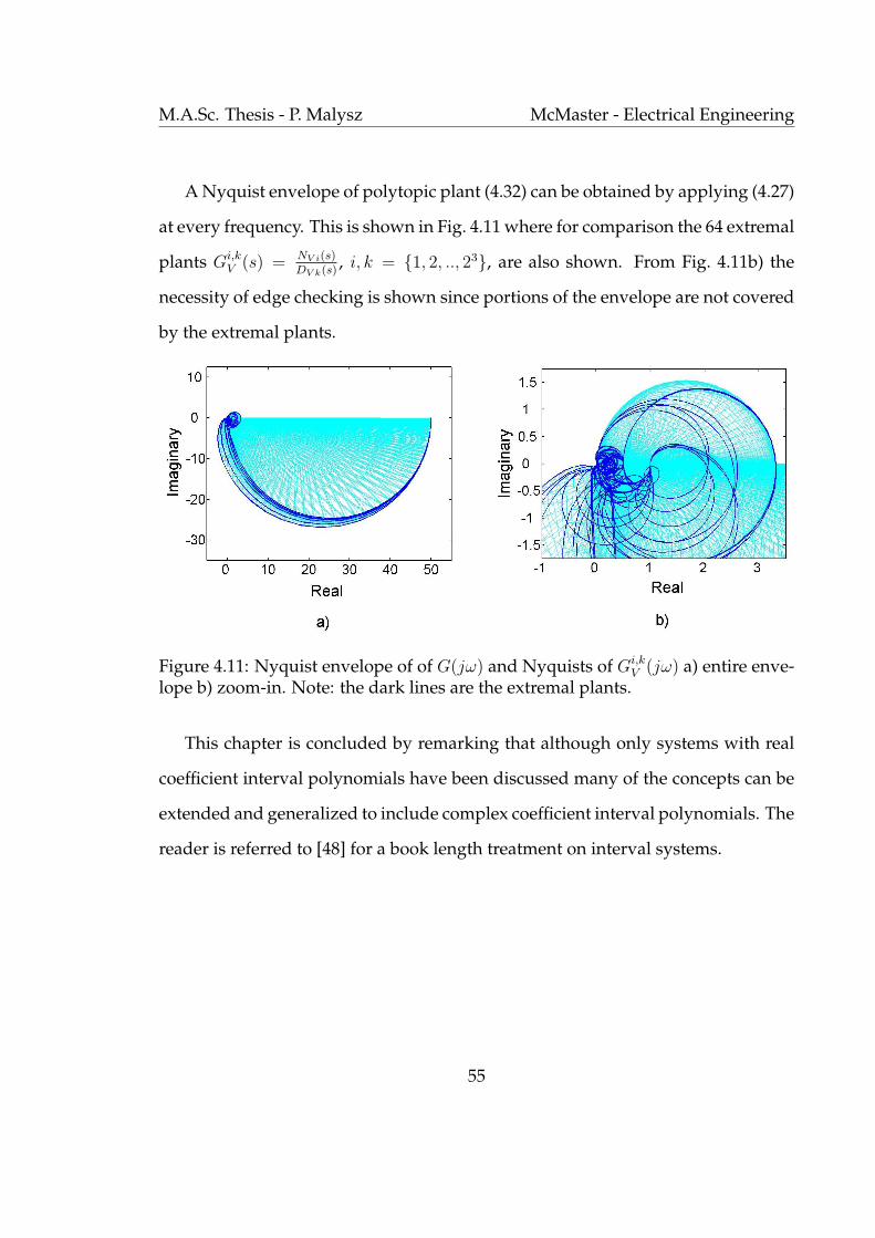
M.A.Sc. Thesis - P. Malysz McMaster - Electrical Engineering
A Nyquist envelope of polytopic plant (4.32) can be obtained by applying (4.27)
at every frequency. This is shown in Fig. 4.11 where for comparison the 64 extremal
plants Gi,kV (s) = NV i(s)
DV k(s), i, k = {1, 2, .., 23}, are also shown. From Fig. 4.11b) the
necessity of edge checking is shown since portions of the envelope are not covered
by the extremal plants.
Figure 4.11: Nyquist envelope of of G(jω) and Nyquists of Gi,kV (jω) a) entire enve-
lope b) zoom-in. Note: the dark lines are the extremal plants.
This chapter is concluded by remarking that although only systems with real
coefficient interval polynomials have been discussed many of the concepts can be
extended and generalized to include complex coefficient interval polynomials. The
reader is referred to [48] for a book length treatment on interval systems.
55

Chapter 5
Stability of Lur’e-Postnikov Systems
The Lur’e-Postnikov problem, known more simply as the Lur’e problem, is a clas-
sical control problem first formulated in 1944 [53]. It is concerned with the stability
of closed-loop systems composed of a linear plant following by a non-linear feed-
back element. A Single-Input-Single-Output (SISO) example of such a system is
shown in Fig. 5.1 where G(s) is a LTI plant and Φ(·) a nonlinear feedback element.
An attractive approach to deduce stability of such closed-loop systems is to make
assumptions on the non-linear element and then analyze the linear part G(s) using
classical linear system methods.
Figure 5.1: Lur’e-Postnikov block diagram
56

M.A.Sc. Thesis - P. Malysz McMaster - Electrical Engineering
One of the early attempts to deduce stability of Lur’e systems was Aizerman’s
conjecture in 1949. It is first noted that a non-linear element Φ(·) belongs to sector
[a, b], if the following holds:
a ≤ Φ(x, t)
x≤ b (5.1)
Aizerman’s conjecture was that if the feedback system is globally asymptoti-
cally stable for all constant linear feedback gains of the form Φ(x, t) = kx with
k ∈ [a, b], then the non-linear Lur’e-Postnikov system is stable for all time invari-
ant nonlinear elements Φ(·) in sector [a, b]. Unfortunately this conjecture is false in
general.
In 1957 another conjecture was made by Kalman. Suppose Φ(·) is a memory-
less time-invariant and continuously differentiable nonlinearly that belongs to an
incremental sector [a, b], i.e.
(i) Φ(0) = 0
(ii) a ≤ Φ(x1)− Φ(x2)
x1 − x2
≤ b (5.2)
Kalman’s conjecture is similiar to Aizerman’s conjecture with the exception that
the non-linear element Φ(·) is memoryless and belongs to an incremental sector
[a, b]. However, this conjecture is also false in general.
Although both conjectures are false, the notion of assuming sector or incremen-
tal sector restrictions on the nonlinear element are still useful for deriving stability
conditions for Lur’e-Postnikov systems. The rest of the chapter will focus on var-
ious sufficient stability conditions assuming different restrictions on the non-linear
feedback element.
57

M.A.Sc. Thesis - P. Malysz McMaster - Electrical Engineering
5.1 Input-Output Passivity
Assuming the nonlinear feedback element Φ(x, t) is a first-third quadrant non-
linearity, i.e. belonging to sector [0,∞], input-output passivity theory can be used
to show stability of the closed-loop system in Fig. 5.1. Before the relevant stability
condition is stated some preliminaries on passivity theory will be discussed.
5.1.1 Passive and Strictly Passive Systems
The general idea behind input-output passivity is concerned with showing that
the increase in stored energy in a system is less than or equal to the input energy,
where the input energy can be defined by the input and output signals.
Consider a system with input u, output y, internal states x and non-negative
energy function V that satisfies (5.3), where y∗u denotes external power. Such a
system can only store, release or consume energy, it cannot produce it.
V (x(T ))− V (x(0)) ≤∫ T
0
y∗u dt (5.3)
Assuming V (x(0)) = 0 in (5.3) the following definitions can be realized for a
system S with input u and output y [54] [55]:
The system S is passive from u to y if for all u and all T > 0:
〈y, u〉T ≥ 0 (5.4)
where
〈y, u〉T =
∫ T
0
y∗u dt (5.5)
58

M.A.Sc. Thesis - P. Malysz McMaster - Electrical Engineering
The system S is strictly passive from u to y if there exists ε > 0 such that for all
u and all T > 0:
〈y, u〉T ≥ ε(〈y, y〉T + 〈u, u〉T ) (5.6)
A resistor is an example of a strictly passive component since it only consumes
energy. Capacitors and inductors are examples of passive components since they
only store and release energy.
A strictly passive system also has the property that it has finite L2-gain, i.e. for
a system with input u and output y, supu∈L2‖y‖2/‖u‖2 is finite [54].
Proof: Using (5.6), the Cauchy-Schwartz inequality 〈y, u〉2T ≤ 〈y, y〉T 〈u, u〉T and
‖y‖2 = limT→∞√〈y, y〉T the following can be obtained
ε(〈y, y〉T + 〈u, u〉T ) ≤ 〈y, u〉T ≤√〈y, y〉T
√〈u, u〉T ≤ ‖y‖2‖u‖2 (5.7)
Hence ε〈y, y〉T ≤ ‖y‖2‖u‖2, letting T →∞ gives
‖y‖2 ≤ 1
ε‖u‖2 (5.8)
5.1.2 Passivity Stability Theorem
A feedback system, like the one illustrated in Fig. 5.2, that can be decomposed into
two elements is closed-loop BIBO stable from u = [u1 u2]T to y = [y1 y2]
T provided
one element (eg. S1) is strictly passive and the other (eg. S2) is passive [56].
59

M.A.Sc. Thesis - P. Malysz McMaster - Electrical Engineering
Figure 5.2: Passivity theorem block diagram.
Proof:S1 strictly passive and S2 passive give:
ε(〈y1, y1〉T + 〈e1, e1〉T ) ≤ 〈y, u〉T (5.9)
where
〈y, u〉T = 〈y1, u1〉T + 〈y2, u2〉T= 〈y1, u1 − y2〉T + 〈y2, u2 + y1〉T (5.10)
= 〈y1, e1〉T + 〈y2, e2〉T
Substituting e1 = u1 − y2 in (5.9) yields
〈y1, y1〉T + 〈y2, y2〉T + 〈u1, u1〉T ≤ 2〈y2, u2〉T +1
ε〈y, u〉T (5.11)
Using Cauchy Schwartz inequality and 〈y2, y2〉〈u2, u2〉 ≤ 〈y, y〉〈u, u〉 leads to
〈y, y〉T ≤ 2〈y2, u2〉T +1
ε〈y, u〉T ≤
(2 +
1
ε
) √〈y, y〉T
√〈u, u〉T (5.12)
Finally letting T →∞ gives ‖y‖2 ≤(2 + 1
ε
) ‖u‖2 and the theorem is proven.
60

M.A.Sc. Thesis - P. Malysz McMaster - Electrical Engineering
Returning to the Lur’e-Postnikov problem in Fig. 5.1, a first-third quadrant
non-linear feedback element in sector [0,∞] is passive since xΦ(x, t) ≥ 0. Stability
is thus achieved provided the linear part G(s) is a strictly passive system. Note
this is only a sufficient stability condition.
5.1.3 Passivity of Linear Systems
A stable linear transfer function G(s) is passive if and only if it is positive real
(PR) [27] i.e.
Re[G(jω)] ≥ 0, ∀ω > 0 (5.13)
This is equivalent to stating that phase of G(s) is in the range of −π/2 and π/2.
Proof: Assuming G(s) is passive its output is y , its input is u where u(t) = 0
when t /∈ [0, T ] the following is obtained using Parseval’s Theorem.
0 ≤∫ T
0
y(t)u(t) dt =
∫ ∞
∞y(t)u(t) dt =
1
2π
∫ ∞
∞Y (jω)U∗(jω) dω (5.14)
Since Y (jω) = G(jω)U(jω) and G(s) is a transfer function of a real system it follows
that
0 ≤ 1
π
∫ ∞
0
Re[G(jω)]|U(jω)|2 dω (5.15)
This equality holds provided that Re[G(jω)] ≥ 0, which is both a necessary and
sufficient condition.
A stable linear transfer function G(s) is strictly passive or dissipative if and
only if it is strictly positive real (SPR) [27] i.e.
Re[G(jω)] > 0, ∀ω > 0 (5.16)
61

M.A.Sc. Thesis - P. Malysz McMaster - Electrical Engineering
The proof is similar to the previous case where the strict passivity property of
ε∫ T
0u(t)u(t) dt ≤ ∫ T
0y(t)u(t) dt with ε > 0 replaces the leftmost inequality in (5.14).
Using the theorem stated in the previous section with stable linear systems
leads to a small phase condition. That is a combination of a passive linear sys-
tem with a strictly passive one have combined phase that is always between ±π,
hence stability is assured.
5.2 On-Axis Circle Theorem
By placing finite sector restrictions on the nonlinear feedback element Φ(x, t) an
application of the small gain theorem can lead to stability conditions on G(s) that
are more relaxed than strict passivity of G(s).
5.2.1 Small Gain Approach
Consider Φ(x, t) to be in sector [−r, r] and G(s) a stable transfer function, then
stability of Fig. 5.1 via the small gain theorem is assured if [55]
supω∈<
|G(jω)| < 1r
(5.17)
The condition in (5.17) is satisfies if the Nyquist plot of G(s) is inside a circle
with centre at the origin that has radius 1r. More useful conditions can be obtained
by allowing arbitrary sectors on Φ(x, t). Using a loop transformation discussed in
the next section leads to the well known on-axis circle criterion [55] [57].
62

M.A.Sc. Thesis - P. Malysz McMaster - Electrical Engineering
5.2.2 Loop transformation
Assume Φ(x, t) lies in an arbitrary sector [a, b], where b > a and define
K =a + b
2, R =
b− a
2(5.18)
The loop transformation shown in Fig. 5.3a) allows the small gain theorem to be
used on the system shown in Fig. 5.3b) where the inputs retain their boundedness
and the feedback element [Φ(x, t)−K] is in sector [−R, R].
Figure 5.3: On-axis circle theorem loop transformation.
63

M.A.Sc. Thesis - P. Malysz McMaster - Electrical Engineering
Applying the small gain theorem to Fig. 5.3b) stability is assured if G(s)1+KG(s)
is
stable and
supω∈<
| G(jω)1+KG(jω)
| < 1
R(5.19)
Expression (5.19) is equivalent to
R < infω∈<
| 1G(jω)
+ K| (5.20)
Which is geometrically equivalent to the Nyquist plot of 1G(jω)
being bound away
from a circle defined by {z ∈ C : |z+K| ≤ R}. Transforming (5.20) through z 7→ 1/z
yields that the Nyquist plot of G(jω), for ab > 0 , must be bounded away from the
circle {z ∈ C : |z + b+a2ab| ≤ b−a
2ab}which intersects the real axis at−1/a and−1/b. This
transformation is illustrated in Fig. 5.4. For a < 0 < b the Nyquist plot of G(jω)
must be contained in the circle {z ∈ C : |z+ b+a2ab| ≤ b−a
2ab}. Assuming 0 = a < b yields
infω∈< Re[G(jω)] > −1b
as the stability condition which is less restrictive than (5.16).
In all cases−1/K is also bounded away from G(jω) thus G(ω)1+KG(jω)
is stable if G(s) is
stable. Although it has been stated that G(s) is open-loop stable the circle theorem
can be extended to handle unstable plants, e.g. the reader is referred to [55].
Using the results of this section the on-axis circle theorem can be stated as fol-
lows. For open-loop stable G(s) with non-linear dynamic feedback Φ(x, t) in sec-
tor [a, b], b > a > 0, closed loop stability is assured if the Nyquist plot of G(jω) is
bounded away and does not encircle a disk that is centered on the real axis and
intersects it at −1/a and −1/b [55].
64

M.A.Sc. Thesis - P. Malysz McMaster - Electrical Engineering
−3 −2 −1 0 1 2 3−3
−2
−1
0
1
2
3
Real
Imag
inar
y
−3 −2 −1 0 1 2 3−3
−2
−1
0
1
2
3
Real
Imag
inar
y
−a −b
___G(s)
G(s)
__ b
__ a
1
−1 −1 −K
a) b)
R
Figure 5.4: On-axis circle theorem test a) graphical interpretation of equation (5.20)b) transformed through z 7→ 1/z. Here G(s) = s2+6s+100
0.35s2+8s+200, a = 0.5 and b = 1.5.
5.3 Off-Axis Circle Theorem
The stability conditions on G(s) can be further relaxed if the non-linear feedback el-
ement Φ(·) is assumed to be memoryless, continuous and in an incremental sector
[k1, k2], meaning it is a static non-linearity with a bounded derivative. By revisiting
passivity theory with the aid of a multiplier concept, the off-axis circle theorem [58]
can be derived. This theorem applies to static non-linear elements that lie in an ar-
bitrary incremental sector [k1, k2], where k2 > k1. If k2 > k1 > 0 the non-linear
element becomes monotonic.
65

M.A.Sc. Thesis - P. Malysz McMaster - Electrical Engineering
5.3.1 Passivity with Multipliers
The multiplier approach transforms the Lur’e-Postnikov problem to the form shown
in either Fig. 5.5a) or b). Stability is then shown, via passivity stability theorem, by
ensuring G(s)Z(s) is strictly passive and either ΦZ−1 or Z−1Φ is passive. Since the
inverse of a passive operator is passive, Z−1Φ and Φ−1Z are equivalently passive.
To ensure boundedness of inputs Zu2 and Z−1u1 the multiplier Z(s) is typically
chosen to be a transfer function where the order of the numerator is the same as
the denominator.
Figure 5.5: Lur’e-Postnikov problem with multipliers
In deriving the off-axis circle theorem the multiplier Z(s) is chosen to have the
following form [58]
Z(s) =N∏
n=0
s + αn
s + βb
(5.21)
where
0 < α0 < β0 < α1 < β1 < ... (5.22)
or
0 < β0 < α0 < β1 < α1 < ... (5.23)
66

M.A.Sc. Thesis - P. Malysz McMaster - Electrical Engineering
The multiplier given in (5.21) is composed of alternating poles and zeros on the
negative real axis. If (5.22) holds then Z(s) is said to be in RL, that is it can be made
up of a network of resistors and inductors [59]. An RC network results for Z(s)
if (5.23) holds [59]. Note if Z(s) in RC then Z−1(s) in RL and vice versa [59]. The
notation ZRL and ZRC will be utilized to denote whether Z(s) is in RL or RC.
Consider a memoryless non-linearity Φ(·) that belongs to the incremental sec-
tor [0,∞], i.e. a monotonic static incrementally positive function. If G(s)Z(s) is
SPR, where Z(s) is defined in (5.21) and assuming either (5.22) or (5.23) then the
feedback system is stable.
Proof:
Note the following proof has been developed by the thesis author since it is not
explicitly given in [58].
Case a) 0 < α0 < β0 < α1 < β1 < ...
Here Z ∈ ZRL and Z−1 ∈ ZRC and using Fig. 5.5a) passivity of ΦZ−1 assures
stability. To show passivity of ΦZ−1, the multiplier Z−1 must first be rewritten in
its RC Foster expansion form [59]. This is done by performing a partial fractions
expansion on the inverse of (5.21)
Z−1(s) = 1 +N∑
n=0
λn
s + σn
, λn ≥ 0, σn > 0 (5.24)
It can be shown that (5.24) followed by an incrementally positive Φ(·) yields
passive ΦZ−1. The proof is lengthy and technical thus the reader is referred to
Lemma 3a of [57].
Case b) 0 < β0 < α0 < β1 < α1 < ...
Here Z ∈ ZRC and Z−1 ∈ ZRL and using Fig. 5.5b) passivity of Z−1Φ assures
67
M.A.Sc. Thesis - P. Malysz McMaster - Electrical Engineering
stability. Since Z−1Φ and Φ−1Z are equivalently passive, Φ(·)−1 also incrementally
positive, and Z(s) able to take the form shown in (5.24), Lemma 3a of [57] is again
utilized to show passivity of Φ−1Z and futhermore system stability.
Alternatively using Fig. 5.5a) it can also be shown that a combination of a ZRL
operator followed by an incrementally positive operator Φ(·) is also passive [60].
The previously stated theorem is useful if it is easy to show that for a given
G(s), a multiplier Z(s) of the form (5.21) exists such that G(s)Z(s) is SPR. Such a
multiplier of the form (5.21) has been proven to exist provided the Nyquist plot
of G(jω) is to the right of a line that passes through the origin [58]. For a detailed
explanation of the proof see [58]. A heuristic explanation is given as follows.
Assume the Nyquist plot of G(jω) is to the right of a line that passes through
the origin making an angle θ with the imaginary axis, therefore the following in-
equality is obtained.
−π
2− θ < arg(G(jω)) <
π
2− θ (5.25)
For a given frequency range ω ∈ [ωa, ωb], positive constants ε1 and ε2 exist such that
−π
2+ ε1 < arg(G(jω)) + θ <
π
2− ε2 (5.26)
Using Lemma 1 of [58] yields a Z ∈ ZRL, for 0 < θ < π2, or a Z ∈ ZRC , for
−π2
< θ < 0, such that
| arg(Z(jω))− θ| ≤ ε, ω ∈ [ωa, ωb] (5.27)
where 0 < ε < min(ε1, ε2). Combining (5.26) and (5.27) yields (5.28) and futhermore
68

M.A.Sc. Thesis - P. Malysz McMaster - Electrical Engineering
strict-passivity of G(s)Z(s).
−π
2< −π
2+ ε1 − ε ≤ arg(G(jω)Z(jω)) ≤ π
2− ε2 + ε <
π
2. (5.28)
The multiplier acts by providing the necessary phase lead (Z ∈ ZRL) or lag (Z ∈ZRL) in the frequency range ω ∈ [ωa, ωb] to ensure G(s)Z(s) is SPR.
Using the results of this section one is able to conclude the following about
a Lur’e-Postinikov problem. If Φ(·) is a memoryless monotonic non-linearity in
incremental sector [0,∞] and the Nyquist plot of G(s) is to the right of a line that
passes through the origin, then the closed loop feedback system is stable.
The theorem can be extended to arbitrary incremental sectors by performing
the loop transformations shown in the next section.
5.3.2 Loop Transformations
Assume the feedback element Φ(·) lies in incremental sector [0, k2], k2 > 0, and the
Nyquist plot of G(s) is to the right of a line that passes through the point − 1k2
. The
loop transformation in Fig. 5.6a) yields a new feedback system in Fig. 5.6b) with
bounded inputs, plant Gb(s) = G(s)+ 1k2
and feedback Φb(·) denoted by the dashed
box. Looking at the output-to-input relationship of Φb(·), Φ−1(·) is in incremental
sector [− 1k2
,∞], thus Φ−1b (·) and Φb(·) are both in incremental sectors [0,∞]. Since
the Nyquist plot of Gb(jω) is to the right of a line that passes through the origin the
results of the previous section show stability.
69

M.A.Sc. Thesis - P. Malysz McMaster - Electrical Engineering
Figure 5.6: Incremental sector [0, k2] loop transformation.
For an arbitrary incremental sector [k1, k2], k2 > k1, an additional loop trans-
formation shown in Fig. 5.7a) is performed to yield the bounded input system in
Fig. 5.7b). Here Φb(·) is denoted by the dashed box in Fig. 5.7a), in Fig. 5.7b) Φc(·)represents the lower dashed box and Gc(s) represents the upper dashed box. Since
Φ−1(·) is in incremental sector [ 1k2
, 1k1
], Φb(·) can be shown to be in incremental sec-
tor [ k1k2
k2−k1,∞] and furthermore Φc(·) in incremental sector [0,∞].
70
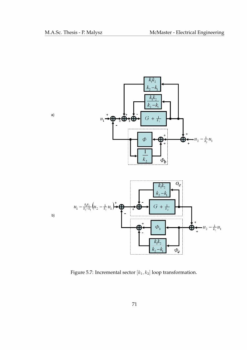
M.A.Sc. Thesis - P. Malysz McMaster - Electrical Engineering
Figure 5.7: Incremental sector [k1, k2] loop transformation.
71

M.A.Sc. Thesis - P. Malysz McMaster - Electrical Engineering
Note that Gc(s) can be represented as
Gc(s) =k2 − k1
k22
· k2G(s) + 1
k1G(s) + 1=
k2
1 + k2G(s)+
k1k2
k2 − k1
(5.29)
The transformation defined in (5.29) operates such that, for k1 < 0 < k2, a Nyquist
plot of G(jω) that is contained in an off-axis circle touching the real axis at − 1k1
and − 1k1
results in the Nyquist plot of Gc(s) to be to the right of a line intersecting
the origin [58]. For 0 < k1 < k2, the Nyquist plot of G(s) must be bounded away
from the off-axis circle. Like before, stability is proven using the arguments of the
previous section. Since the centre of the off-axis circle is not restricted, infinitely
many different off-axis circles can be formed given a specific k1 and k2.
Finally one can conclude the needed off-axis circle theorem for the nonlinear
Lur’e-Postinikov problem. For open-loop stable G(s) with memoryless non-linear
feedback Φ(·) belonging to incremental sector [k1, k2], closed-loop stability is as-
sured provided, for 0 < k1 < k2, the Nyquist plot of G(jω) is bounded away and
does not encircle an off-axis circle that intersects the real axis at − 1k1
and − 1k1
[58].
A graphical example is shown in Fig. 6.1
5.4 Other Methods
Researching Lur’e-Postinikov problems one finds the scientific literature is rich in
content. Therefore this chapter is concluded by briefly mentioning other poten-
tially useful methods.
72

M.A.Sc. Thesis - P. Malysz McMaster - Electrical Engineering
The well known Popov criterion [55] is suited for showing stability with mem-
oryless time-invariant nonlinearities belonging to sector [0, b]. It is based on a pas-
sivity with multipliers approach and has a corresponding graphical test to show
stability for a given G(s). The graphical test is based on the Popov plot, a graph
of Re(G(jω)) versus ωIm(G(jω)). Stability is shown when the Popov plot is to the
right of a line intersecting −1b. The nonlinearity Φ(·) need not be monotonic, how-
ever it must has lower sector equal to zero. Another limitation is that the Popov
criterion is limited to strictly proper plants for G(s) and also requires the derivative
of the input to be bounded.
Another result obtained by Narendra and Cho applies to static odd-monotonic
nonlinearities [61]. It is also a passivity with multipliers approach where it is
shown that a specific multiplier Zodd(s) preserves passivity when combined with
a static odd-monotonic function in incremental sector [0,∞]. However there is no
graphical test or systematic way to show that for a specific plant G(s), there ex-
ists a Zodd(s) such that G(s)Zodd(s) is SPR hence the theorem is difficult to apply in
practice.
More recently Materassi et al. have proposed that the on-axis circle criterion
can be relaxed to include static hyperbolic type sector non-linearities [62]. Stability
is shown using a Lyapunov-based argument to show the closed-loop system is
globally bounded. However strict properness of the linear part G(s) is required.
Finally it is noted that the stability conditions presented in this chapter are only
sufficient and not necessary.
73

Chapter 6
Teleoperation Stability Analysis
The theory presented in the previous two chapters will be utilized to perform a
stability analysis on the teleoperation block diagram that concluded chapter three.
Different types of generalized tranparency objectives are considered in this chap-
ter. The first section presents stability conditions assuming simple first-order force
filtering with static non-linear scaling of either force or position. Stability is ana-
lyzed using a combination of an off-axis circle criterion with the Nyquist envelope
of interval plants systems obtained by using Kharitonov plants [63]. The second
section focuses on LTI filtered mappings of position and force where the exact
stability regions are obtained by analyzing the closed-loop characteristic equa-
tion. The third section considers combinations of mixed non-linear/LTI filtered
mappings where stability is shown utilizing the off-axis circle criterion with the
Nyquist envelope of interval polytopic plants. The final section shows that re-
formulating the off-axis circle criterion to be utilized with bode envelopes as ex-
plained in [64] is a more conservative approach when compared to using Nyquist
envelopes.
74

M.A.Sc. Thesis - P. Malysz McMaster - Electrical Engineering
6.1 Static Nonlinear Feedback
It is possible to convert the teleoperation block diagram in Fig. 3.1b) to a nonlinear
Lur’e-Postnikov type problem shown in Fig. 5.1 by assuming that one of the two
mappings is linear, i.e. by considering linear position/nonlinear force or nonlinear
position/linear force scaling combinations. Furthermore, assuming force filters
Hfh = Hfe = Cs+C
and position filters H ′xm = H ′
xs = 1, the linear part would reduce
to
G(s) =m1s
2 + b1s + k1
m2s2 + b2s + k2
=Ze
Zh + Zt
(6.1)
with the nonlinear feedback element
Φ(·) =
κf (·)κ−1p κp(·) linear
κ−1p (·)κf κf (·) linear
(6.2)
and an exogenous inputs u2 = 0 and u1 ∈ L∞ defined as
u1 =
F ∗h − ρ− Zh+Zt
1+C−1sρe , κp(·) linear
−F ∗hκfZe
+ 1+C−1sκfZe
ρ + Zh+Zt
κfZeρe , κf (·) linear
(6.3)
where m1 ≥ 0, b1 ≥ 0, k1 ≥ 0 represent environment impedance parameters and
m2 = mh + mt > 0, b2 = bh + bt > 0, k2 ≥ 0 represent the combined impedance
parameters of the hand and virtual tool.
6.1.1 Passivity approach
Assuming the non-linear element Φ(·) is passive, for example first-third quadrant
non-linearities which satisfy xΦ(x) ≥ 0, the passivity theorem presented in section
75

M.A.Sc. Thesis - P. Malysz McMaster - Electrical Engineering
5.1.2 can be used. This leads to a sufficient stability condition of strict positive
realness of the linear part (6.1), i.e.
infω∈<
Re(−m1ω
2 + b1jω + k1
−m2ω2 + b2jω + k2
)> 0 (6.4)
The condition in (6.4) is shown in Appendix A.1 to be equivalent to
b1b2 >(√
m1k2 −√
m2k1
)2
(6.5)
which must be satisfied for all possible combinations of hand and environment
parameters. In practice, allowing all possible environment and hand impedances
results in large perturbations in G(s) making stability, if possible, challenging to
guarantee. However, it is reasonable to limit the parameters to some known ranges
that can be determined based on the application. In Table 6.1, a hypothetical exam-
ple of such bounds for soft-tissue telemanipulation is given. The ranges in Table 6.1
are comparable to those found in [10] and [9].
Table 6.1: Parameter Ranges for Hand and Environment
Mass (kg) Damping (Nsm−1) Stiffness (Nm−1)Ze 0.01–0.2 5–50 10-1000Zh 0-0.3 0–100 20-1000
Using (6.5) and (6.1) with a desired hypothetical virtual tool mass of mt =
0.4 kg, and the data in Table 6.1, the minimum level of virtual tool damping needed
for G(s) to be SPR is bt > 15
(√0.01(20)−
√0.7(1000)
)2
= 135 Nsm−1. Assum-
ing negligible tool mass, mt ≈ 0, yields bt > 57 Nsm−1. Clearly such levels of
76

M.A.Sc. Thesis - P. Malysz McMaster - Electrical Engineering
tool damping can result in extremely sluggish system response and degrade the fi-
delity of soft-tissue telemanipulation. Due to the rather excessive conservatism of
the passivity-based condition, alternative stability conditions must be considered.
6.1.2 Circle criterions with Nyquist envelope
The on/off axis circle criterions [55, 58] presented in the previous chapter can pro-
duce a far less conservative sufficient stability condition at the expense of more
restriction on the nonlinear element. The on-axis criterion assumes that the non-
linear mapping Φ(·) belongs to a sector, see (5.1), whereas the off-axis criterion
assumes Φ(·) belongs to an incremental sector, see (5.2). Note that if Φ(·) lies in in-
cremental sector [a, b] it lies in sector [k1, k2], where k1 ≥ a and k2 ≤ b, hence the
on-axis criterion can also be applied to incremental sector nonlinearities. Assum-
ing incremental sector [a, b] with b > a > 0 yields Φ(·) to be monotonic. Both circle
criterions conclude stability if the Nyquist plot of the linear part is outside of a
circle which intersects the negative real axis at − 1a
and −1b. Since the on-axis test
requires the circle to have its centre on the real axis, the off-axis criterion yields a
larger incremental sector range [a, b], as shown in Fig. 6.1.
Using a transformation that maps an off-axis circle to the imaginary axis a nu-
merical stability test can be obtained. Using the following transformation
H(s) =G(s) + 1
2( 1
a+ 1
b)− dj − r
G(s) + 12( 1
a+ 1
b)− dj + r
(6.6)
r =
√d2 +
1
4
(1
a− 1
b
)2
, d ∈ <
77
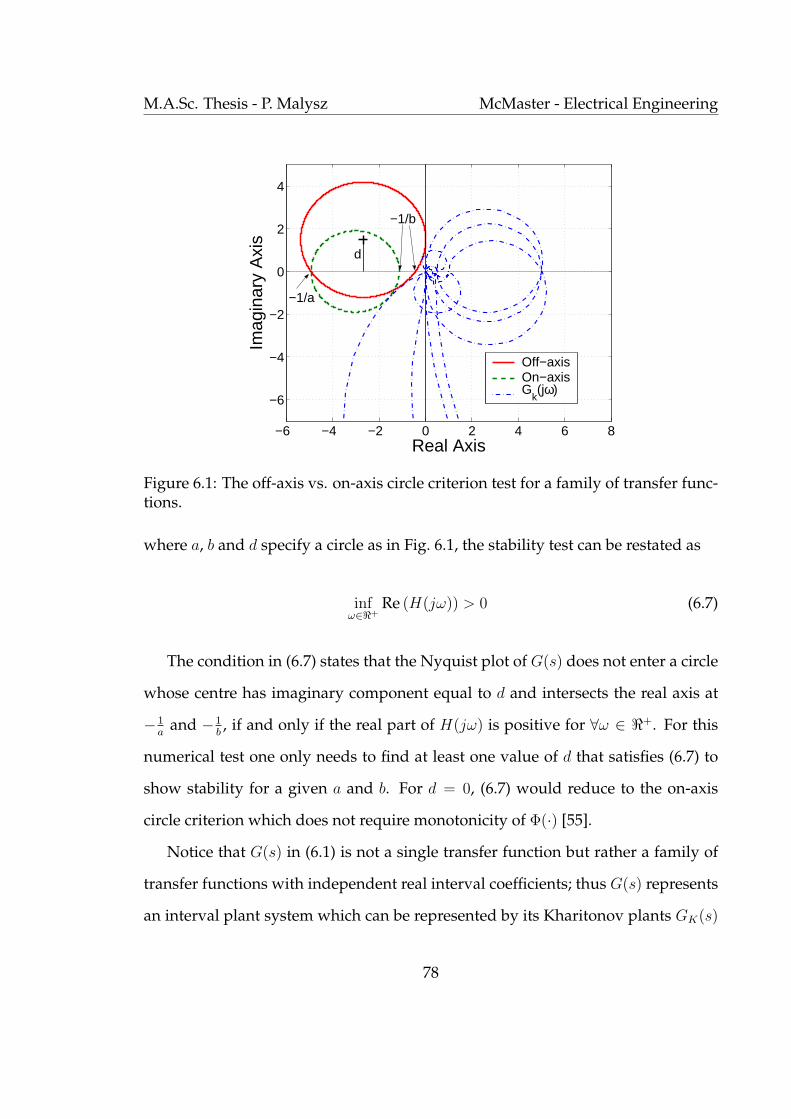
M.A.Sc. Thesis - P. Malysz McMaster - Electrical Engineering
−6 −4 −2 0 2 4 6 8
−6
−4
−2
0
2
4
Real Axis
Imag
inar
y A
xis
Off−axisOn−axisG
k(jω)
d
−1/a
−1/b
Figure 6.1: The off-axis vs. on-axis circle criterion test for a family of transfer func-tions.
where a, b and d specify a circle as in Fig. 6.1, the stability test can be restated as
infω∈<+
Re (H(jω)) > 0 (6.7)
The condition in (6.7) states that the Nyquist plot of G(s) does not enter a circle
whose centre has imaginary component equal to d and intersects the real axis at
− 1a
and −1b, if and only if the real part of H(jω) is positive for ∀ω ∈ <+. For this
numerical test one only needs to find at least one value of d that satisfies (6.7) to
show stability for a given a and b. For d = 0, (6.7) would reduce to the on-axis
circle criterion which does not require monotonicity of Φ(·) [55].
Notice that G(s) in (6.1) is not a single transfer function but rather a family of
transfer functions with independent real interval coefficients; thus G(s) represents
an interval plant system which can be represented by its Kharitonov plants GK(s)
78

M.A.Sc. Thesis - P. Malysz McMaster - Electrical Engineering
defined in (4.11) [3]. H(s) in (6.6) is also an interval plant system whose coefficients
may be complex and depend linearly on the coefficients of G(s). To determine
if (6.7) is satisfied for the interval system H(s), it is sufficient to check if (6.7) is
satisfied for the 16 Kharitonov plants GK(s). The proof of this lies in the fact that
for ω ∈ <+ the outer Nyquist envelope of the interval system G(s) can be found
from the union of the Nyquist plots of GK(s), e.g. see section 4.2.2 [3]. Therefore
if the Nyquist envelope of G(s) lies outside the circle specified by a, b and d, then
Re(H(jω)) > 0 for ∀ω ∈ <+. The benefit of using (6.7) is in that it is no longer a
graphical test as is shown in Fig 6.1.
Given a, an upper value of b, b ≥ a, can be found by searching through the
two dimensional space of b ∈ <+ and d ∈ < using (6.7) as a stability constraint.
This has been done using both the on-axis and off-axis circle criterions with the
intervals specified in Table 6.1. Fig. 6.2 shows the results of such an analysis with
the virtual tool parameters of mt = 0.4 kg and bt = 10 Nsm−1. Among the design
parameters, the virtual tool damping has the biggest impact on the closed-loop
stability. This can be observed in Fig. 6.3 where the stability margins derived from
the off-axis circle criterion have increased at the expense of a higher tool damping.
It is observed in Fig 6.2 and Fig. 6.3 that for small values of lower incremental
sector a, the upper incremental sector b plateaus. This corresponds to the case
where the Nyquist envelope of (6.1) is to the right of a line that intersects the
negative-real axis. For larger values of a, there a exists a critical value of a such
that the Nyquist envelope of (6.1) is outside a circle that touches the origin. This
case in turn corresponds to the Nyquist plot of 1/G(jω) being to the right of a line
intersecting the negative real axis.
79
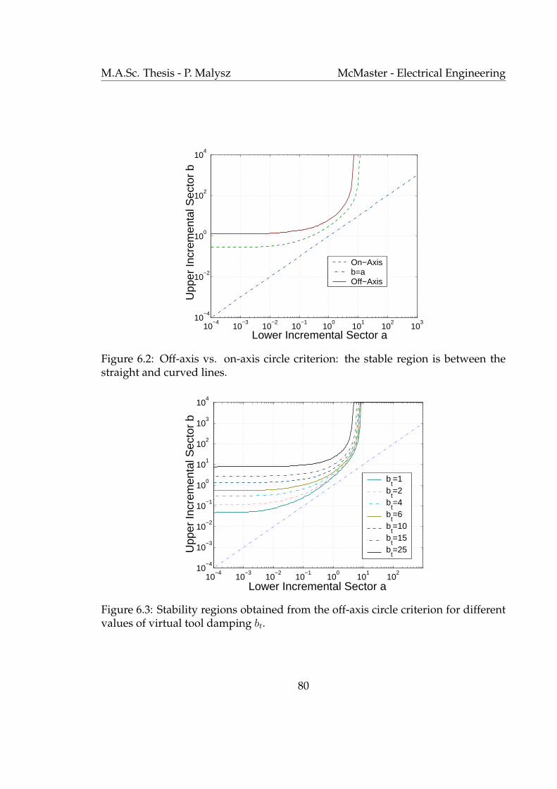
M.A.Sc. Thesis - P. Malysz McMaster - Electrical Engineering
10−4
10−3
10−2
10−1
100
101
102
103
10−4
10−2
100
102
104
Lower Incremental Sector a
Upp
er In
crem
enta
l Sec
tor
b
On−Axisb=aOff−Axis
Figure 6.2: Off-axis vs. on-axis circle criterion: the stable region is between thestraight and curved lines.
10−4
10−3
10−2
10−1
100
101
102
10−4
10−3
10−2
10−1
100
101
102
103
104
Lower Incremental Sector a
Upp
er In
crem
enta
l Sec
tor
b
bt=1
bt=2
bt=4
bt=6
bt=10
bt=15
bt=25
Figure 6.3: Stability regions obtained from the off-axis circle criterion for differentvalues of virtual tool damping bt.
80
M.A.Sc. Thesis - P. Malysz McMaster - Electrical Engineering
When applying the test (6.7) for on-axis circles, where d = 0 in (6.6), the coef-
ficients in H(s) are all real. Therefore a stability analysis can be made more com-
putationally efficient by using condition (6.5) with the sixteen transformed H(s)
plants. This eliminates the need of explicitly finding the Nyquist plots of GK(s).
The off-axis stability analysis can be made more computationally efficient by using
the results of an on-axis analysis as starting points for a maximum upper incremen-
tal sector search. One may also exploit monotonicity of the upper sector b curves to
further increase computational efficiency. Monotonicity is expected since by fixing
b and increasing a one makes the circle in Fig. 6.1 smaller.
6.2 LTI Filtered Mappings
Assuming linear scalings of force κf (·) = κf and position κp(·) = κp, the teleop-
eration block diagram in Fig.3.1b) reduces to a linear system with plant (6.8) and
unity feedback. Note HZt = H ′xm( C
s+C)Zt.
G(s) =H ′
xm
H ′xs
·Hfe
kf
kpZe
H ′xm
Cs+C
Zt + HfhZh
(6.8)
Furthermore the filters are assumed to be represented as LTI transfer functions
with fixed numerator and denominator polynomials taking the form
H∼(s) =HN∼ (s)
HD∼ (s)(6.9)
81

M.A.Sc. Thesis - P. Malysz McMaster - Electrical Engineering
Thus the linear plant (6.8) is rewritten as
G(s) =H ′N
xmH ′Dxs
H ′DxmH ′N
xs
·H ′D
xmHDfhH
Nfe(C
−1s + 1)kf
kpZe
HDfhH
DfeH
′NxmZt + H ′D
xmHDfeH
Nfh(C
−1s + 1)Zh
(6.10)
The closed loop characteristic polynomial of G(s)/[1 + G(s)] is the following
C(s)= PZe(s)κf
κpZe + PZh(s)Zh + PZt(s)Zt (6.11)
PZe(s) =HNfe(s)H
Dfh(s)H
′Dxs (s)H ′N
xm(s)(C−1s+1) (6.12)
PZh(s)=HDfe(s)H
Nfh(s)H
′Nxs (s)H ′D
xm(s)(C−1s+1) (6.13)
PZt(s)=HDfe(s)H
Dfh(s)H
′Nxs (s)H ′N
xm(s) (6.14)
The characteristic polynomial (6.11) can be rewritten to take the form below
C(s) = a0(q) + a1(q)s + ... + an(q)sn (6.15)
q = [me, be, ke, mh, bh, kh,mt, bt]T (6.16)
where the coefficients ai(q) depend linearly on q; the mass, spring, and damper
parameters of Ze, Zh and Zt. Assuming intervals on q results in (6.11) being
a polytopic polynomial. Stability can then be shown using the origin exclusion
tests described in section 4.1.2. Specifically the phase stability condition (4.10)
can be utilized. A stability analysis was performed using three different sets of
force/position filters with the intervals in Table 6.1, virtual tool mass of 0.4 kg,
various fixed values of virtual tool damping and assuming force/position scaling
such that κf
κp= 1.
82

M.A.Sc. Thesis - P. Malysz McMaster - Electrical Engineering
Stability regions have been obtained by searching through the parameter space
of the filters and obtaining binary images that show stable or potentially unstable
regions. The potentially unstable regions involve at least one element in the inter-
val family such that the teleoperation system would become unstable or marginally
stable. By choosing various fixed values of virtual tool parameters only 26 vertex
polynomials were required to perform the analysis. However the virtual tool pa-
rameters could also be chosen to lie in intervals, therefore 28 vertex polynomials
would be required in such an analysis. It is also noted that when performing the
computational analysis one must take care when discretizing the frequencies ω,
since a coarse discretization may yield false stability regions. This occurs since an
origin exclusion test between two frequency steps that would show potential in-
stability is not performed. These false stability regions can manifiest themselves
as jagged edges or ridges near the stable/potentially unstable boundary where a
smooth continuous boundary may otherwise be expected.
6.2.1 Additional force filtering
The first set of filters used for stability analysis was additional second-order filter-
ing of the force signals. This may be desired to remove unwanted sensor noise.
The corresponding filters are
H ′xm = H ′
xs = 1 (6.17)
Hfe = Hfh = Cs+C
· ω2n
s2+2ζωns+ω2n
(6.18)
83

M.A.Sc. Thesis - P. Malysz McMaster - Electrical Engineering
The characteristic polynomial that determines stability in this cases is given by
C(s) = ( 1ω2
ns2 + 2 ζ
ωns + 1)Zt + Zh + Ze (6.19)
from which it is evident that the additional force filtering gives the virtual tool
higher order dynamics. Stability regions have been graphed in Fig. 6.4 for various
values of virtual tool damping and filter parameters. It should also be noted that
assuming fixed virtual tool parameters results in the independence of the coeffi-
cients of the characteristic polynomial (6.19). Hence the stability can be investi-
gated considering only the four Kharitonov polynomials given in (4.4).
102
103
0.2
0.4
0.6
0.8
1
1.2
1.4
1.6
1.8
Natural Frequency ωn (rad/s)
Dam
ping
rat
io ζ
bt= 1
bt= 2
bt= 4
bt= 6
bt= 10
bt= 15
Stable PotentiallyUnstable
Figure 6.4: Additional second-order force filtering stability regions at different lev-els of virtual tool damping bt.
84

M.A.Sc. Thesis - P. Malysz McMaster - Electrical Engineering
6.2.2 Force compensator mapping
The second set of filters analyzed are
H ′xm = H ′
xs = 1 (6.20)
Hfh = Cs+C
(6.21)
Hfe = Cs+C
· τ1s+1τ2s+1
(6.22)
where a force compensator mapping is used that amplifies or attenuates higher
frequency environment forces, depending on the values of τ1 and τ2. The corre-
sponding characteristic polynomial is given by
C(s) = (τ1s + 1)Ze + (τ2s + 1)(Zh + Zt) (6.23)
10−3
10−2
10−1
100
101
102
10−3
10−2
10−1
100
101
Time constant τ2 (s)
Tim
e co
nsta
nt τ
1 (s)
bt= 1
bt= 2
bt= 4
bt= 6
bt= 10
bt= 15
PotentiallyUnstable
Stable
PotentiallyUnstable
Figure 6.5: Force compensator filter stability regions at different levels of virtualtool damping bt.
85
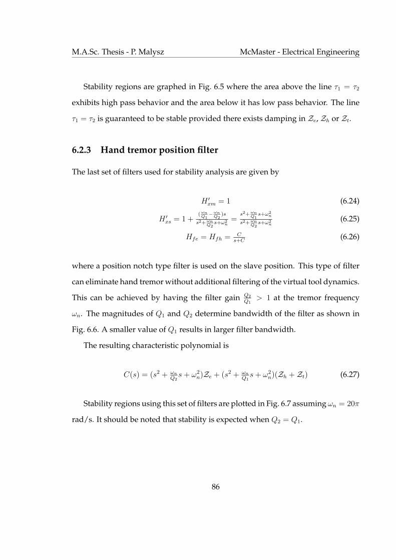
M.A.Sc. Thesis - P. Malysz McMaster - Electrical Engineering
Stability regions are graphed in Fig. 6.5 where the area above the line τ1 = τ2
exhibits high pass behavior and the area below it has low pass behavior. The line
τ1 = τ2 is guaranteed to be stable provided there exists damping in Ze, Zh or Zt.
6.2.3 Hand tremor position filter
The last set of filters used for stability analysis are given by
H ′xm = 1 (6.24)
H ′xs = 1 +
( ωnQ1−ωn
Q2)s
s2+ ωnQ2
s+ω2n
=s2+ ωn
Q1s+ω2
n
s2+ ωnQ2
s+ω2n
(6.25)
Hfe = Hfh = Cs+C
(6.26)
where a position notch type filter is used on the slave position. This type of filter
can eliminate hand tremor without additional filtering of the virtual tool dynamics.
This can be achieved by having the filter gain Q2
Q1> 1 at the tremor frequency
ωn. The magnitudes of Q1 and Q2 determine bandwidth of the filter as shown in
Fig. 6.6. A smaller value of Q1 results in larger filter bandwidth.
The resulting characteristic polynomial is
C(s) = (s2 + ωn
Q2s + ω2
n)Ze + (s2 + ωn
Q1s + ω2
n)(Zh + Zt) (6.27)
Stability regions using this set of filters are plotted in Fig. 6.7 assuming ωn = 20π
rad/s. It should be noted that stability is expected when Q2 = Q1.
86
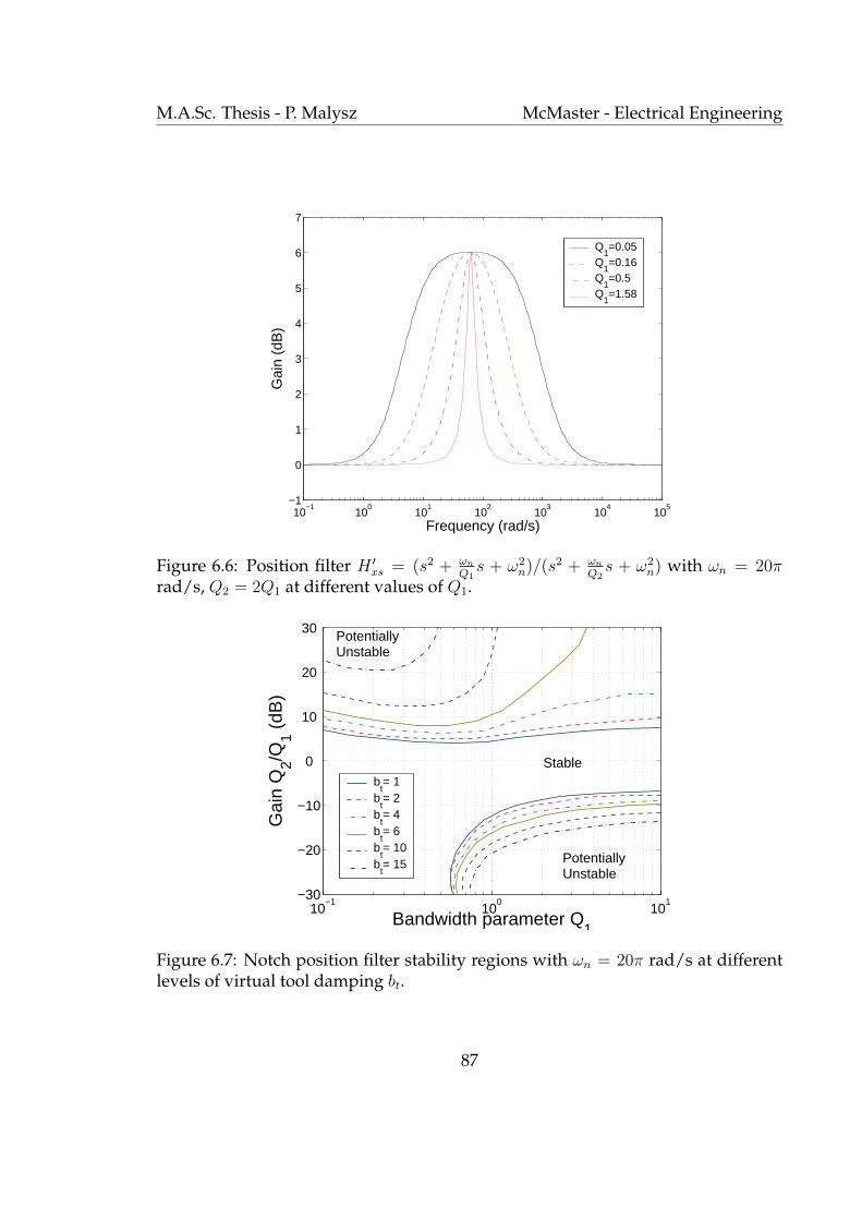
M.A.Sc. Thesis - P. Malysz McMaster - Electrical Engineering
10−1
100
101
102
103
104
105
−1
0
1
2
3
4
5
6
7
Frequency (rad/s)
Gai
n (d
B)
Q1=0.05
Q1=0.16
Q1=0.5
Q1=1.58
Figure 6.6: Position filter H ′xs = (s2 + ωn
Q1s + ω2
n)/(s2 + ωn
Q2s + ω2
n) with ωn = 20πrad/s, Q2 = 2Q1 at different values of Q1.
10−1
100
101
−30
−20
−10
0
10
20
30
Bandwidth parameter Q1
Gai
n Q
2/Q1 (
dB)
bt= 1
bt= 2
bt= 4
bt= 6
bt= 10
bt= 15
PotentiallyUnstable
PotentiallyUnstable
Stable
Figure 6.7: Notch position filter stability regions with ωn = 20π rad/s at differentlevels of virtual tool damping bt.
87

M.A.Sc. Thesis - P. Malysz McMaster - Electrical Engineering
6.3 Mixed Non-Linear/LTI Filtered Mappings
Using LTI filtered mappings with either nonlinear force or nonlinear position scal-
ing the teleoperation block in Fig. 3.1b) can once again be converted to a Lur’e type
problem shown previously in Fig. 5.1. This is achieved by defining G(s) to be
G(s) =GN (s)
GD(s)=
PZe(s)Ze
PZh(s)Zh + PZt(s)Zt
(6.28)
Φ(·) to be (6.2) as before and the exogenous inputs u2 = 0 and u1 ∈ L∞ to be
u1 =
HfhF∗h − ρ− HfhZh+HZt
H′xm
ρe , κp(·) linear
−HfhF ∗hκf HfeZe
+κ−1
f ρ
HfeZe+
(HfhZh+HZt)ρe
κf H′xmHfeZe
, κf (·) linear(6.29)
where PZe(s), PZh(s), and PZt(s) have been defined previously in (6.12), (6.13) and
(6.14). Robust stability can once again be investigated using the sufficient condi-
tions of the off-axis circle theorem with nonlinear feedback element Φ(·) and the
Nyquist envelope of the interval plant system (6.28). Since the linear plant G(s)
contains independent polytopic polynomials GN (s) and GD(s), the Nyquist enve-
lope of such a polytopic plant can be found using the method discussed in sec-
tion 4.3.2 where edge checking must be performed [2].
Once a Nyquist envelope of the linear plant (6.28) is obtained an analogous
graphical test to that of Fig. 6.1 can be used to show that an off-circle circle is out-
side the Nyquist envelope of G(s) to conclude nonlinear stability. When a numer-
ical stability test is desired, the transformation defined previously in (6.6) can be
applied to the points that make up the Nyquist envelope of (6.28) to yield stability
88

M.A.Sc. Thesis - P. Malysz McMaster - Electrical Engineering
condition (6.7). The necessity of edge checking results in a computationally expen-
sive procedure when compared to the Kharitonov polynomials approach used for
independent coefficient interval polynomials.
As an example, stability analysis is performed for teleoperation system involv-
ing the LTI filters defined in (6.24)-(6.26), the interval ranges in Table. 6.1 with
nonlinear force scaling κf (·) and linear position scaling κp. This can reveal po-
tential trade-offs between hand-tremor filtering specifications and nonlinear en-
hanced force mapping specifications. The results of such an analysis are shown
in Fig. 6.8 where nonlinear sector stability regions are found for various values of
position filtering bandwidth using a virtual tool impedance of Zt = 0.4s2 + 15s.
The guaranteed stability region is between the straight line b = a and the curves
obtained for each Q value.
The application of position filtering introduces the potential for instability even
for linear scalings of force and position, hence disconnected nonlinear sector sta-
bility regions can result as shown in Fig. 6.8. These unstable linear gains are easily
found by observing where the Nyquist envelope of (6.28) intersects the negative
real axis. The analysis in Fig. 6.8 shows that for a certain notch position filter band-
width a minimum incremental sector stability region can exist, for example by
choosing lower sector a = 1.
89

M.A.Sc. Thesis - P. Malysz McMaster - Electrical Engineering
10−1
100
101
10−1
100
101
102
Lower Incremental sector a
Upp
er In
crem
enta
l sec
tor
b
10−1
100
101
Lower Incremental sector a
Q1=0.2
Q1=0.3
Q1=0.45
Q1=0.6
a=b
Q1=2.4
Q1=1.2
Q1=0.9
Q1=0.6
a=b
a) b)
Figure 6.8: Stability regions from off-axis circle criterion with notch position filter-ing at ωn = 18π rad/s with gain Q2
Q1= 5 and varying bandwidth. a) 0.2 ≤ Q1 ≤ 0.6
b) 0.6 ≤ Q1 ≤ 2.4.
6.4 Conservatism of using Bode envelopes
Tan and Atherton have transformed the off-axis circle theorem to be used with
Bode envelopes of the linear plant G(s) [64]. In their approach, the non-linear feed-
back element Φ(·) is represented by a range of complex gains that lie inside a circle
on the gain plane. To obtain this gain plane circle, the off-axis circle on the Nyquist
plane is mapped through z 7→ −1/z. For stability the equation ΦG(jω) + 1 = 0
90
M.A.Sc. Thesis - P. Malysz McMaster - Electrical Engineering
is investigated. The gain-phase relationship of the gain-plane circle describing Φ
is used in combination with the Bode envelope of G(s) to show stability. For an
open-loop stable plant G(s) this is done by ensuring for all gain/phase ranges of
Φ in combination with G(s) have combined gain less than one when the combined
phase is −180◦. For more details on the application of this approach the reader
should consult [64].
The approach in [64] is equivalent to using the original off-axis circle criterion
with a Nyquist envelope that is obtained from a Bode envelope. Hence the Nyquist
templates at each frequency are overbounded since they are assumed to have a
sector shape. An example of this is shown in Fig. 6.9a) using example (4.32) from
section 4.3.2. Complete Nyquist envelopes are also shown in Fig. 6.9b). Apply-
ing the off-axis circle theorem to the overbounded Nyquist envelope would result
in smaller incremental sector stability ranges since smaller off-axis circles are al-
lowed. Despite this conservatism an advantage of using this approach is that it is
less computationally expensive. As was discussed in section 4.3, obtaining a Bode
envelope of a polytopic plant only requires the use of its vertex polynomials, thus
expensive edge checking is not needed. Another advantage is that stability can po-
tentially be shown for open-loop unstable plants since it may be possible to keep
track of the number of encirclements when using a Bode envelope [64]. Ultimately,
since the Bode envelope approach is more conservative, an extensive teleoperation
stability analysis was not explored for nonlinear feedback stability.
91

M.A.Sc. Thesis - P. Malysz McMaster - Electrical Engineering
Figure 6.9: Nyquist overbounding a) Nyquist template at ω = 30 rad/s b) Nyquistenvelopes. The overbounded Bode envelope approach is in lighter (green) colourwhereas the true Nyquist envelope is in darker (red) colour.
92

Chapter 7
Psychophysics
To design any enhanced generalized mapping one typically should apply psy-
chophysical theory and methods to validate that the mapping actually enhances
performance/perception. The first section of this chapter will cover some basic
psychophysical theory and methods that can be applied in many types of hu-
man factors studies. The second section discusses generalized mapping design
and specifically gives design criteria for a nonlinear perception enhancing force
mapping. The third section presents psychophysical experiments used to validate
the enhanced nonlinear force mapping design.
93

M.A.Sc. Thesis - P. Malysz McMaster - Electrical Engineering
7.1 Psychophysics Theory and Methods
7.1.1 Theory
Psychophysics is a science that deals with human perception that uses aspects of
the physical sciences and as well as psychology. Central to psychophysics is the
concept of a sensory threshold. Two different thresholds can be defined: absolute
thresholds (RL for the German Reiz Limen) define the smallest amount of stimu-
lus that can be detected, whereas differential thresholds (DL for German Differenz
Limen) define the smallest perceivable difference between two stimuli [4]. The
DL is sometimes referred to as the just-noticeable-difference (jnd) between two stim-
uli. The stimulus (φ) refers to a quantity that is measured in the physical domain.
The sensation (ψ) refers to the psychological quantity the observer experiences [4].
Psychophysical laws describe the relationship between stimulus (φ) and sensation
(ψ) [4]. Different senses would have different ψ − φ relationship since the physical
mechanisms of each sense are different. A review of the physical capabilities of
different human senses is given in Chapter 2 of [4]. A classical mathematical rela-
tionship between sensation and stimuli is Fechner’s law (7.1) which first appeared
in his 1860 publication Elements of Psychophysics. It was not until the 1950’s that
alternative ψ−φ relationships were explored. Steven’s power law (7.2) [65] has be-
come another popular mathematical representation. The constants k and a would
be specific to the sensory modality and stimulus conditions.
Fechner’s Law ψ = k ln φ (7.1)
Steven’s Power Law ψ = kφa (7.2)
94

M.A.Sc. Thesis - P. Malysz McMaster - Electrical Engineering
Any experiment to measure sensation typically involves human responses, ther-
efore sensory response laws describe the relationship between sensation and the sen-
sory response given by the observer. An ideal sensation-sensory response relation-
ship would be linear with unity gain, in which case the human is able to ideally
give a response about their sensation magnitude without distortion. When consid-
ering groups of people, on average the sensation-sensory response relationship is
linear with unity [4]. In the context of this thesis an ideal sensory response law is
assumed. The assumed two-stage sensory theory is thus shown in Fig. 7.1.
Figure 7.1: Assumed two-stage sensory theory showing how the psychophysicaland sensory response laws intervene, figure from [4].
95

M.A.Sc. Thesis - P. Malysz McMaster - Electrical Engineering
Classical psychophysical threshold theory defines the sensory threshold (both
RL and DL) to be a step function that fluctuates over time and under different stim-
ulus conditions. In this theory a momentary step-threshold is assumed to exist at
the point of observervation. This fluctuation smooths out the step function into
a sigmoidal curve. Thus experimental results would expect to resemble that of
Fig. 7.2, where a yes indicates the observer has perceived the stimulus. A popular
model of this sigmoidal curve is that it is the integral of a Gaussian distribution
that varies among individuals and depends on the sensory modality and stimu-
lus conditions. This response curve is referred to as the psychometric function
and describes the subject’s performance under different stimulus intensities. This
function and its range are task-dependent. For example it is possible to obtain a
psychometric function with ranges other than 0-100%. Examples of this will be
explained in the next section.
Figure 7.2: Psychometric function from classical threshold theory, figure from [4].
96
M.A.Sc. Thesis - P. Malysz McMaster - Electrical Engineering
It must be noted that this classical threshold theory does not fully explain the
sensory response process since it does not take into account the psychological na-
ture and expectations of the human observer. Improved theories such as that of
the Theory of Signal Detection (TSD) are more prevalent in the psychophysics lit-
erature today. An overview of TSD in psychophysics can be found in Chapters 5-8
in [4]. Ultimately TSD also results in sigmoidal psychometric functions that take
into account the expectations and criteria of the observer [4]. These other theories
and theories that explain the relationships between the psychometric function and
psychophysical laws are beyond the scope of work in this thesis. The important
point is that these theories use the concept of a psychometric function. This psy-
chometric function quantifies the sensory threshold and describes the probability
of a response under different stimuli conditions. By choosing a point on the psy-
chometric function one chooses a DL or RL point with an associated probability.
7.1.2 Methods
Psychophysics experiments are typically performed to obtain data about the psy-
chometric function. Ideally it is desirable for different stimuli to be presented at
the same place, time and for the same duration to remove space and temporal bias
errors. This is usually impossible, especially in the case of measuring differen-
tial thresholds. For stimuli presented in different places, spatial counterbalancing
where stimuli are equally distributed among the different places is used to reduce
spatial bias errors. Additionally order bias caused from predictable stimuli can
also be problematic, hence random ordering is typically used. Any experimental
method must minimize these and other unwanted bias errors.
97

M.A.Sc. Thesis - P. Malysz McMaster - Electrical Engineering
The method of constant stimuli or method of constants is a classical experimen-
tal technique [4]. This method seeks to obtain the entire psychometric function by
presenting repeated stimuli where a wide range of stimuli is chosen. The range
covers stimuli from levels that are almost never detected to levels that are almost
always detected. An associated probability value is found experimentally on many
points on the psychometric function through repeated measurements. Typically
curve fitting techniques are used to obtain the psychometric function. For absolute
thresholds the 50% level (RL50) is typically chosen as the threshold value since the
experimental psychometric function typically resembles that of Fig. 7.2.
For differential thresholds a comparison stimulus can be compared to a stan-
dard stimulus. The standard stimulus is always known to the observer and is of
fixed value. The varying comparison stimulus is judged to be either of greater or
lesser intensity. A hypothetical psychometric function for such a differentiation
discrimination experiment is shown in Fig. 7.3.
Figure 7.3: Hypothetical psychometric function obtained from method of constantsfor a discrimination task with a known standard, figure from [4].
98

M.A.Sc. Thesis - P. Malysz McMaster - Electrical Engineering
In this case the 50% level corresponds to the Point of Subjective Equality (PSE)
where no discrimination is expected due to guessing. An experimental PSE that
deviates greatly from the standard stimulus value is indicative of unwanted bias
errors. Two differential thresholds are defined, an upper threshold, typically DLu =
P75 − PSE and a lower threshold usually DLl = PSE − P25. Both correspond
to a correct identification performance level of 75%, note when comparing only
two stimuli guessing performance is at worst 50%. Typically the upper and lower
threshold are averaged, i.e. DL75 = 12(DLl + DLu).
The method of constants can also be used with a forced choice paradigm [4].
Instead of yes/no or greater/less responses at each trial, multiple stimuli are pre-
sented where the observer has to identify which interval contains the stimulus.
For RL experiments only one interval has the stimulus, for DL experiments only
one interval contains the comparison and the rest have intensity equal to the stan-
dard. Note in DL experiments the observer does not know which stimulus is the
standard. The worst case performance is the inverse of the number of intervals,
i.e. a two alternative forced choiced task (2AFC) has a psychometric function with
performance ranging from 50-100%. A hypothetical example is shown in Fig. 7.4.
0 1 2 3 4 50.5
0.6
0.7
0.8
0.9
1
∆X (stimulus level)
% C
orre
ct
Figure 7.4: Hypothetical psychometric function for a 2AFC discrimination task.Two thresholds (at 75% and 90%) for ∆X can be defined as shown.
99

M.A.Sc. Thesis - P. Malysz McMaster - Electrical Engineering
The method of Limits is another classical method that is considered to be more
efficient that the method of constant stimuli [4]. It seeks to give a single threshold
measurement instead of the entire psychometric function. Unfortunately this tech-
nique is considered unreliable since subject bias exists and the method does not
target a fixed performance level, hence this method will not be discussed in detail.
In many cases the entire psychometric function is not needed since a single
representative point may suffice. In such cases adaptive up-down methods are
more efficient since they concentrate the stimulus level around a chosen point on
the psychometric function [66]. The method is adaptive since future stimulus val-
ues are based on the responses of the observer. Typically correct responses results
in stimulus intensity (or difference for DL experiments) to decrease or step down
(Sdown) and incorrect responses lead to an increase or step up (Sup). The classical
Bekesy threshold tracking method has symmetric step sizes (Sdown = Sup) for in-
correct/correct responses and a step is made after each response [67]. This would
target an equilibrium point with a performance level of 50%, since the probabilities
of moving up and down are equal at the 50% level. For discrimination tasks with
only one standard and only one comparison, the classical up-down method is not
useful since it converges to the PSE.
A Transformed Up-Down Method (TUDM) proposed by Levitt allows conver-
gence to the 70.7% performance level [66]. Symmetric step sizes are assumed
(Sup = Sdown) however the rules for when steps are taken have been transformed.
The TUDM looks at sequences of responses after a step has been made. A sequence
of two consecutive correct responses (++) results in a step-down. An incorrect re-
sponse (−) or a sequence of correct and incorrect (+−) leads to a step-up. The
100
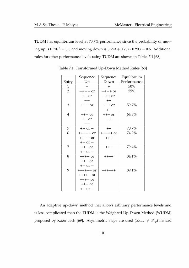
M.A.Sc. Thesis - P. Malysz McMaster - Electrical Engineering
TUDM has equilibrium level at 70.7% performance since the probability of mov-
ing up is 0.7072 = 0.5 and moving down is 0.293 + 0.707 · 0.293 = 0.5. Additional
rules for other performance levels using TUDM are shown in Table. 7.1 [68].
Table 7.1: Transformed Up-Down Method Rules [68]
Sequence Sequence EquilibriumEntry Up Down Performance
1 − + 50%2 −+−− or −+−+ or 55%
+− or −++ or−− ++
3 +−− or +−+ or 59.7%− ++
4 ++− or +++ or 64.8%+− or −+−−
5 +− or − ++ 70.7%6 ++−+− or ++−++ or 74.9%
++−− or ++++− or −
7 ++− or +++ 79.4%+− or −
8 +++− or ++++ 84.1%++− or+− or −
9 +++++− or ++++++ 89.1%++++− or+++− or++− or+− or −
An adaptive up-down method that allows arbitrary performance levels and
is less complicated than the TUDM is the Weighted Up-Down Method (WUDM)
proposed by Kaernbach [69]. Asymmetric steps are used (Sdown 6= Sup) instead
101

M.A.Sc. Thesis - P. Malysz McMaster - Electrical Engineering
of response sequences. Steps are made after single responses and convergence to
performance percentage level p is achieved provided the steps satisfy equilibrium
equation (7.3).
Sup(1− p) = Sdownp (7.3)
For example choosing p = 0.75 results in Sup/Sdown = 3, hence for a correct re-
sponse a step down of one unit is taken and for an incorrect response a three unit
step-up is taken. It has also been shown the WUDM has a small advantage over
TUDM in terms of efficiency and faster convergence [70] [69].
All up-down methods obtain their data by plotting stimulus intensity versus
trial number. Threshold measurements at the chosen performance level are ob-
tained by taking the midpoint value of each run. The midpoint value gives an
single estimate of the threshold with reduced variability. A run is a set of increas-
ing or decreasing steps. Either increasing or decreasing runs are chosen to ensure
independence of the data. The midpoints of the runs yield mean and variance
measurements of the sensory threshold of interest. The starting point can bias the
first few runs, hence they are typically ignored. A priori knowledge and prelimi-
nary experiments can yield good starting points for the up-down methods; even
so the first run should always be ignored. Hypothetical data using the WUDM are
shown in Fig. 7.3. The choice of step size influences both the speed of convergence
and the variability of the data. Large steps have faster convergence but greater
variability, smaller steps have the opposite. An optimal step size that balances the
two should be chosen. Strategies such as initially taking large steps followed by
smaller steps can also easily be employed.
102

M.A.Sc. Thesis - P. Malysz McMaster - Electrical Engineering
Figure 7.5: Hypothetical data from WUDM with Sup/Sdown = 3. The dark circlesare threshold measurements and the dotted line their average.
7.2 Enhanced Mapping Design
7.2.1 Nonlinear force mapping
The design of any non-linear force mapping will be a task-dependent procedure.
In soft-environment telemanipulation it might be desired to improve performance
in a stiffness or softness discrimination task. Force and stiffness discrimination
has been shown experimentally to obey Weber’s Law [43], [4]. Weber’s Law
states that the just-noticeable difference (jnd) in stimulus intensity (∆φ) is linearly
proportional to the starting intensity (φ) by a constant factor c:
∆φ = cφ or∆φ
φ= c (7.4)
103

M.A.Sc. Thesis - P. Malysz McMaster - Electrical Engineering
The Weber constant c can therefore be used as a measure of differential sensitivity.
Assuming jnd increments are equally spaced in the sensation domain (ψ), Fech-
ner’s Law (7.1) can be derived from Weber’s Law. To show this one takes the
derivative of (7.1) to yield the expression ∆φ = φk∆ψ. Substituting this express-
ing into (7.4) yields ∆ψ = ck which is constant. Weber’s original work dealt with
the discrimination ability of lifted weights. Fechner, aware of this work sought a
mathematical relationship between sensation (ψ) and stimulus (φ) and proposed
(7.1) to be consistent with Weber’s results.
A force mapping can be used to modify the transmitted forces to improve the
perceptual ability of an individual. For enhanced differential sensitivity the map-
ping (7.5) should satisfy (7.6).
Fh = kf (Fe) (7.5)
∆Fh
Fh
>∆Fe
Fe
orδFh
δFe
>Fh
Fe
(7.6)
Using (7.5), (7.6) can be rewritten as (7.7), where ′ denotes the derivative:
Fek′f (Fe)
kf (Fe)> 1 or
k−1f (Fh)
Fh(k−1f (Fh))′
> 1 (7.7)
For linear mappings of force, (7.7) can only hold with equality and differential
sensitivity cannot be enhanced. Condition (7.7) can be used to enhance sensitivity
over a specified range of environment or hand forces. In particular, force mappings
of the form (7.8) with β > 1 satisfy (7.7) and yield enhanced sensitivity under
Weber’s Law. Diminished sensitivity occurs when β < 1.
Fh = α|Fe|β · sign(Fe) (7.8)
104

M.A.Sc. Thesis - P. Malysz McMaster - Electrical Engineering
7.2.2 Nonlinear Spatial and Filtered Mappings
Nonlinear position mappings can be used to better manage workspace in the tele-
operation system. For example an area of high precision can be defined by having
an appropriate position scaling in that region. This can be achieved through piece-
wise continuous line segments in the position mapping from master to slave. Each
line segment can have a different slope, the connecting regions can also be chosen
to have continuous derivatives to improve continuity.
For controllers that enforce velocity tracking, as opposed to enforcing position
tracking, an appropriate nonlinear velocity mapping can also potentially increase
precision. This can be done by having slow hand velocities scaled less than fast
hand velocities. The proposed controller in this thesis can be made to work in
velocity mode by eliminating virtual tool damping. However, doing so is done at
the expense of teleoperation system stability. Therefore this velocity generalized
mapping would require an improved controller.
Filtered mappings can improve teleoperation performance by filtering unwan-
ted system noise. For example, filtering force sensor signals can improve system
performance by not conveying those disturbances to the operator. Surgeon hand
tremor frequencies have been measured to be in the 8-12Hz range [34]. Using sim-
ple low-pass filters produce an undesirable sluggish response, hence frequency
band notch type filters like those presented in section 6.2.3 can be utilized to pre-
serve high frequency content. Reducing hand tremor can potentially improve hu-
man performance in fine telemanipulation. Further research is required to deter-
mine the types of filtered force mappings that can improve human perception.
However some insight can be gained by studying the frequency responses of the
105

M.A.Sc. Thesis - P. Malysz McMaster - Electrical Engineering
different haptic sensors in the skin. These responses are shown in Fig. 7.6 which
has been obtained from [5]. Further psychophysics research and human factors
experiments are required to determine more specific design criteria for enhanced
nonlinear spatial and filtered mappings.
This section is concluded by commenting that the issue of human adaptation
and learning to any enhanced mapping design should be addressed. Also in a
practical implementation it may be desirable to switch between different enhanced
mappings on-the-fly based on the desired task to be performed. This switching
has potential negative implications on perception, performance and practical ease
of use. All these issues require further human factors studies to effectively use
enhanced generalized mappings.
Figure 7.6: Haptic tactile and kinesthetic receptors. Figure modified from [5].
106
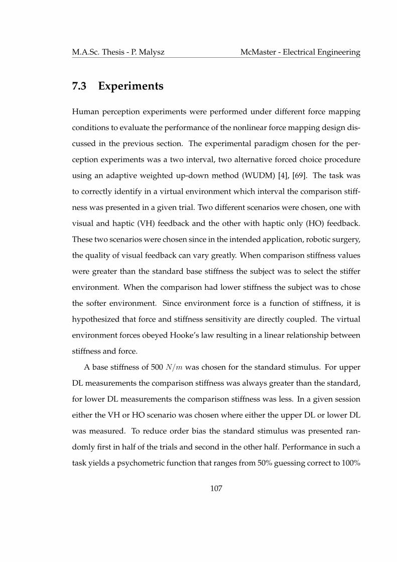
M.A.Sc. Thesis - P. Malysz McMaster - Electrical Engineering
7.3 Experiments
Human perception experiments were performed under different force mapping
conditions to evaluate the performance of the nonlinear force mapping design dis-
cussed in the previous section. The experimental paradigm chosen for the per-
ception experiments was a two interval, two alternative forced choice procedure
using an adaptive weighted up-down method (WUDM) [4], [69]. The task was
to correctly identify in a virtual environment which interval the comparison stiff-
ness was presented in a given trial. Two different scenarios were chosen, one with
visual and haptic (VH) feedback and the other with haptic only (HO) feedback.
These two scenarios were chosen since in the intended application, robotic surgery,
the quality of visual feedback can vary greatly. When comparison stiffness values
were greater than the standard base stiffness the subject was to select the stiffer
environment. When the comparison had lower stiffness the subject was to chose
the softer environment. Since environment force is a function of stiffness, it is
hypothesized that force and stiffness sensitivity are directly coupled. The virtual
environment forces obeyed Hooke’s law resulting in a linear relationship between
stiffness and force.
A base stiffness of 500 N/m was chosen for the standard stimulus. For upper
DL measurements the comparison stiffness was always greater than the standard,
for lower DL measurements the comparison stiffness was less. In a given session
either the VH or HO scenario was chosen where either the upper DL or lower DL
was measured. To reduce order bias the standard stimulus was presented ran-
domly first in half of the trials and second in the other half. Performance in such a
task yields a psychometric function that ranges from 50% guessing correct to 100%
107

M.A.Sc. Thesis - P. Malysz McMaster - Electrical Engineering
correct. A difference threshold at 75% correct was chosen and measurements at
this level were obtained using the WUDM by decreasing the stiffness difference
between the comparison and standard by 16 N/m for each correct response, and
increasing it by 48 N/m for each incorrect response. To reduce time effects and
keep the trial time consistent, contact time with each box was at most three sec-
onds. This was enforced by removing haptic feedback after 3 seconds had elapsed
from initial contact.
The linear spring forces were mapped through three different mappings as
shown in Fig. 7.7, with the mapping equations given in Table 7.2. To reduce sub-
ject bias, the enhanced and diminished mappings were scaled such that all three
mappings felt similar to each other and that they shared a common point at 8 N
to yield the same force range. The three mappings were interleaved in the same
session and presented in random order to further reduce any bias errors. Each ses-
sion consisted of a total of 120 trials where 40 trials of data was recorded for each
mapping. With 40 trials, the WUDM yielded approximately 6 useful threshold
measurements per mapping. The starting value for the comparison stiffness was
chosen to be 692 N/m for upper DL measurements, 356 N/m for lower DL mea-
surements and was the same for each force mapping in a given session. Eleven
volunteers were recruited to participate in the psychophysics experiments with
ages ranging from 22 to 26, of which eight were male and three were female. Each
volunteer completed four sessions, two for the VH scenario and two for the HO
scenario, for a total of 480 trials. Prior to each session each subject had a practice
period to get familiar with the experimental procedures.
108
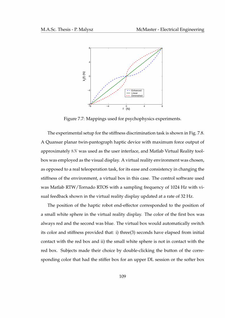
M.A.Sc. Thesis - P. Malysz McMaster - Electrical Engineering
−8 −4 0 4 8−8
−4
0
4
8
f (N)
k f(f)
(N)
EnhancedLinearDiminished
Figure 7.7: Mappings used for psychophysics experiments.
The experimental setup for the stiffness discrimination task is shown in Fig. 7.8.
A Quansar planar twin-pantograph haptic device with maximum force output of
approximately 8N was used as the user interface, and Matlab Virtual Reality tool-
box was employed as the visual display. A virtual reality environment was chosen,
as opposed to a real teleoperation task, for its ease and consistency in changing the
stiffness of the environment, a virtual box in this case. The control software used
was Matlab RTW/Tornado RTOS with a sampling frequency of 1024 Hz with vi-
sual feedback shown in the virtual reality display updated at a rate of 32 Hz.
The position of the haptic robot end-effector corresponded to the position of
a small white sphere in the virtual reality display. The color of the first box was
always red and the second was blue. The virtual box would automatically switch
its color and stiffness provided that: i) three(3) seconds have elapsed from initial
contact with the red box and ii) the small white sphere is not in contact with the
red box. Subjects made their choice by double-clicking the button of the corre-
sponding color that had the stiffer box for an upper DL session or the softer box
109
M.A.Sc. Thesis - P. Malysz McMaster - Electrical Engineering
Figure 7.8: Setup for psychophysics experiments. Note: The dashed box representsthe location of the selection dialog box under the haptics only experiments wherevisual feedback is removed.
for a lower DL session. To reduce spatial bias subjects where instructed to inter-
act with only the top surface of the virtual environment. For the VH scenario, the
selection dialog box was entirely below the virtual box as is shown in Fig. 7.8 by
ignoring the dashed rectangle. For the HO scenario visual feedback was removed
by placing the selection dialog box so that it blocked the top portion of the virtual
environment, as illustrated in Fig. 7.8 via the dashed rectangle. The bottom por-
tion of the box was left visible to enable the user to identify the color of the box.
Since the position of the haptic device end-effector was still visible, the subjects
were instructed to keep their attention on the computer monitor to strictly enforce
the HO scenario.
110

M.A.Sc. Thesis - P. Malysz McMaster - Electrical Engineering
Experimental results for the stiffness discrimination task are shown in Fig. 7.9,
where for each subject the average of threshold measurements for each mapping
is plotted for both VH and HO scenarios. Despite large variability among the sub-
jects, a trend is seen to support the hypothesis that the proposed nonlinear force
mapping enhances stiffness sensitivity regardless of the presence of visual feed-
back. Specifically under the VH scenario, nine out of eleven subjects had an im-
proved upper DL and eight out of eleven had an improved lower DL under the
enhanced force mapping. For the HO scenario nine out of eleven had an improved
upper DL and another nine out of eleven an improved lower DL. This trend is
also evident from Table 7.2 where the overall average DL and stiffness threshold
among all subjects is given for each experimental condition. Comparing the VH
and HO scenarios, visual feedback improves stiffness discrimination. This result
is in agreement with previous reports in the literature, e.g. see [44]. All threshold
measurements were statistically analyzed using Repeated Measures ANalysis Of
VAriance (ANOVA) [71]. The Repeated Measures ANOVA method is discussed in
Appendix A.2. The resulting analysis is summarized in Table 7.3 based on which
it can be concluded that the experimental results are statistically significant.
Table 7.2: Average Difference Threshold for 75% PerformanceMapping Type Enhanced Linear Diminished
kf (f) 18f 2 · sign(f) f
√8|f | · sign(f)
Upper DL HV (*) 116.1 (616.1) 158.8 (658.8) 189.5 (689.5)Lower DL HV (*) 90.8 (409.2) 110.0 (390.0) 145.1 (354.9)Upper DL HO (*) 235.3 (735.3) 292.8 (792.8) 345.9 (845.9)Lower DL HO (*) 125.8 (374.2) 151.7 (348.3) 172.6 (327.4)
*the corresponding stiffness level is shown in parenthesis.
111

M.A.Sc. Thesis - P. Malysz McMaster - Electrical Engineering
Enhanced Linear Diminished
300
400
500
600
700
800
Com
paris
on S
tiffn
ess
(N/m
)
Enhanced Linear Diminished200
300
400
500
600
700
800
900
1000
1100
a) b)
Figure 7.9: Subject comparison stiffness for 75% performance versus mapping a)Haptics with Vision (HV) scenario b) Haptics Only (HO) scenario
Table 7.3: Repeated Measures ANOVA analysisThreshold All mappings Linear/Enhanced Linear/Diminished
same same sameUpper DL HV p < 0.001 p < 0.01 p < 0.05Lower DL HV p < 0.001 p < 0.05 p < 0.01Upper DL HO p < 0.001 p < 0.001 p < 0.01Lower DL HO p < 0.001 p < 0.05 p < 0.05
112
Chapter 8
Teleoperation Experiments
Teleoperation experiments were performed to validate the generalized mapping
adaptive controller presented in chapter 3. The first section in this chapter presents
the experimental setup used for the telemanipulation experiments. The second
section presents the assumed workspace dynamic model and gives details on how
the controller was implemented. The final section shows experimental results
where non-linear/filtered force/position mappings were utilized.
113

M.A.Sc. Thesis - P. Malysz McMaster - Electrical Engineering
8.1 Experimental Setup
The master/slave experimental setup is shown in Fig. 8.1. Two Quanser panto-
graph mechanisms each with two active axes of motion in the x-y plane have been
employed as master and slave robots. The pantograph devices are actuated by
two direct-drive DC motors attached to the proximal links. Motor shaft torque is
controlled via current controlling power supplies. The shaft angles are measured
by optical encoders with 20, 000 counts per revolution. Two Mini40 force/torque
sensors from ATI Industrial Automation have been attached to the mechanisms
end-effectors to measure the hand and environment interaction forces. Sponge
is used to create the effect of a soft tissue. The control code runs under Matlab
RTW/Tornado VxWorks real-time operating system with a sampling frequency of
2048 Hz. Two PCs were utilized, a Windows based PC was used to program the
controller using Simulink. This PC is connected to a second PC that ran the control
code under VxWorks RTOS to control the master and slave devices.
Figure 8.1: The two-axis experimental setup.
114

M.A.Sc. Thesis - P. Malysz McMaster - Electrical Engineering
8.2 Controller Implementation
The pantograph devices are light, have low-friction and are easily backdrivable.
The mass of the force sensor and end-effector attachments dominate the device
dynamics, hence the master/slave subsystems are modeled as linear decoupled
mass-spring-damper systems, with parametric uncertainty, in the workspace coor-
dinates as shown in Fig. 8.2. Position-dependent variations in the device dynamics
due to nonlinearities are adapted for by the local master/slave controllers. To deal
with the human exogenous force F ∗h , the control law in (3.15) employs a switching
term that can cause unwanted chattering in the control signal. For the experiment
the master controller was modified such that it would adapt for F ∗h by adding it to
the feedforward term (3.20). This is acceptable provided the adaptation is much
faster than the rate of change in F ∗h . The resulting dynamic equation is shown in
(8.1), where γ = m and λ = h for the master subsystem and γ = s and λ = e for the
slave subsystem. Note, xγ0 and yγ0 are the contact points.
Figure 8.2: Dynamic model used for workspace controllers.
115

M.A.Sc. Thesis - P. Malysz McMaster - Electrical Engineering
mγ,x + mλ,x 0
0 mγ,x + mλ,x
xγ
yγ
+
bγ,x + bλ,x 0
0 bγ,x + bλ,x
xγ
yγ
+
kγ,x + kλ,x 0
0 kγ,x + kλ,x
xγ − xγ0
yγ − yγ0
=
Fγ,x
Fγ,y
= Fγ (8.1)
The basic control block diagram for the teleoperation system is shown in Fig. 8.3,
where the workspace variables are vector quantities. The force sensor and joint
angles are filtered to reduce sensor noise and quantization noise. The effect of
quantization noise is small since the encoder resolution is high, hence the position
filter can be omitted. A second-order filter (8.2) was used with ωn = 500π rad/s
for the position filter and ωn = 120π rad/s for the force filter. Angular velocity
was obtained by filtering using (8.3) with ωn = 100π rad/s. All filters used in the
controller implementation were converted to discrete-time filters using the Matlab
c2d function with the ’tustin’ option where a bilinear transformation is utilized.
Figure 8.3: Control block diagram for teleoperation experiments.
116
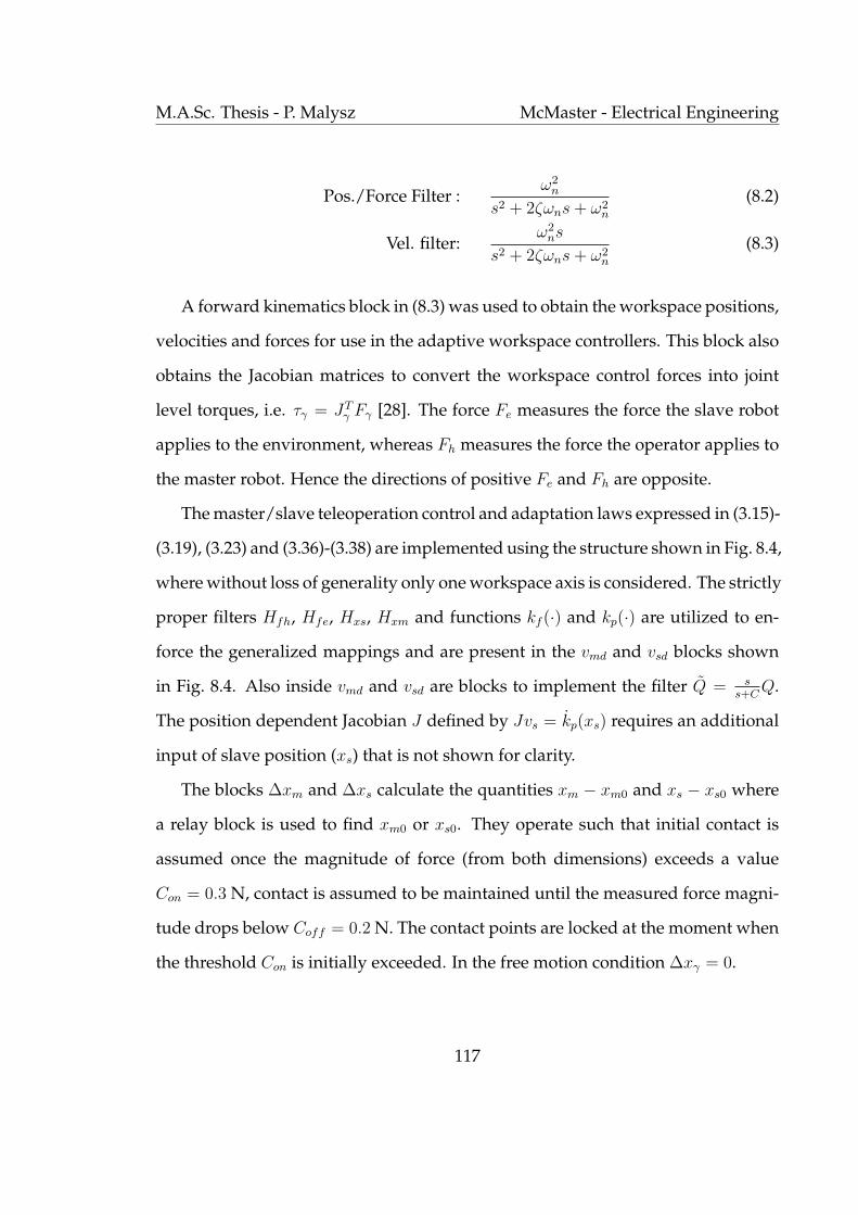
M.A.Sc. Thesis - P. Malysz McMaster - Electrical Engineering
Pos./Force Filter :ω2
n
s2 + 2ζωns + ω2n
(8.2)
Vel. filter:ω2
ns
s2 + 2ζωns + ω2n
(8.3)
A forward kinematics block in (8.3) was used to obtain the workspace positions,
velocities and forces for use in the adaptive workspace controllers. This block also
obtains the Jacobian matrices to convert the workspace control forces into joint
level torques, i.e. τγ = JTγ Fγ [28]. The force Fe measures the force the slave robot
applies to the environment, whereas Fh measures the force the operator applies to
the master robot. Hence the directions of positive Fe and Fh are opposite.
The master/slave teleoperation control and adaptation laws expressed in (3.15)-
(3.19), (3.23) and (3.36)-(3.38) are implemented using the structure shown in Fig. 8.4,
where without loss of generality only one workspace axis is considered. The strictly
proper filters Hfh, Hfe, Hxs, Hxm and functions kf (·) and kp(·) are utilized to en-
force the generalized mappings and are present in the vmd and vsd blocks shown
in Fig. 8.4. Also inside vmd and vsd are blocks to implement the filter Q = ss+C
Q.
The position dependent Jacobian J defined by Jvs = kp(xs) requires an additional
input of slave position (xs) that is not shown for clarity.
The blocks ∆xm and ∆xs calculate the quantities xm − xm0 and xs − xs0 where
a relay block is used to find xm0 or xs0. They operate such that initial contact is
assumed once the magnitude of force (from both dimensions) exceeds a value
Con = 0.3 N, contact is assumed to be maintained until the measured force magni-
tude drops below Coff = 0.2 N. The contact points are locked at the moment when
the threshold Con is initially exceeded. In the free motion condition ∆xγ = 0.
117

M.A.Sc. Thesis - P. Malysz McMaster - Electrical Engineering
a)
b)
Figure 8.4: Adaptive controllers a) master controller b) slave controller
118

M.A.Sc. Thesis - P. Malysz McMaster - Electrical Engineering
The ddt
blocks in Fig. 8.4 are not explicitly used. Instead, expressions ρm+vm and
ρs + kp(xs) are found by defining filters Hfh, Hfe, Hxm, Hxs, defining force mapping
Jacobian Jkf to satisfy JkfHfeFe = kf (HfeFe), using position mapping Jacobian J
and utilizing ˙Q = CQ− CQ when necessary.
In a single axis implementation regressor Ym is defined in (8.4), where the
added fourth element in effect includes exogenous force F ∗h in the adaptation.
The adaptation estimates of the combined mass/hand parameters are also given
in (8.4). For slave adaptation the regressor Ys and associated slave/environment
estimates defined in (8.5) are used. Note here J is a scalar quantity and J ′ = ddxs
J .
Y Tm =
ρm + vm
ρm + vm
∆xm
−1
, Θm =
mm+h
bm+h
km+h
F ∗h
(8.4)
Y Ts =
J−2(ρs + kp(xs)
)− J ′J−3 · vs ·
(ρs + kp(xs)
)
J−2(ρs + kp(xs)
)
J−1∆xs
, Θs =
ms+e
bs+e
ks+e
(8.5)
The form of Ys in (8.5) is necessary to be consistent with (8.1) and the mapped
slave dynamics expressed in (3.13), where it is noted J = ddt
J = ddx
J · dxdt
= J ′ · vs.
This form of Ys required signals xs and vs, which are explicitly shown in Fig. 8.4b).
Finally the implementation of blocks Θm and Θs in Fig. 8.4 use Matlab discrete-time
integrator blocks with upper/lower limits to implement adaptation rule (3.23).
119

M.A.Sc. Thesis - P. Malysz McMaster - Electrical Engineering
This section is concluded by remarking that in a discrete-time implementation
the local force feedback can cause instability in the system. This issue was explored
by Zhu and Salcudean [26] for a controller with simple linear mappings where it
is shown the product of AC must be small enough for stability in a discrete-time
implementation. The stability conditions derived in this thesis are valid for the
continuous-time domain. Using the results from [26], a value of AC small enough
results in a stable discrete-time implementation. It has also been heuristically ob-
served that other parameters that amplify local force-feedback should be kept low
to maintain stability. Conditions for stability for the proposed generalized map-
ping controller in a discrete-time implementation requires further research.
8.3 Experimental Results
Experimental results for the adaptive controllers described in the previous section
and chapter 3 were obtained using the control parameters given in Table 8.1. The
specific limits and gains used for adaptation are given in Table 8.2. The resulting
position and force experimental data were recorded at a rate of 256 Hz.
Table 8.1: Controller ParametersA C Λ Ks,Km Γs,Γm
0.01 kg−1s 80π rad/s 10 s−1 35 Nsm−1 1000-25000000
120

M.A.Sc. Thesis - P. Malysz McMaster - Electrical Engineering
Table 8.2: Adaptation ParametersRange Gain (Γγi)
mm+h 0.1–0.4 kg 1000bm+h 1–20 Ns/m 2000km+h 0-1 N/m 10,000,000F ∗
h -10–10 N 2000ms+e 0.1–0.4 kg 1000bs+e 1–20 Ns/m 20000ks+e 0-1000 N/m 25,000,000
8.3.1 Nonlinear force scaling with filtered position mapping
The first experiment was conducted using the linear position scaling (8.6) and non-
linear monotonic force scaling (8.7) with the filters defined in (8.8)-(8.10). These
filters were previously seen in section 6.2.3. The chosen nonlinear force mapping
was selected to have a narrower incremental sector than the psychophysics exper-
iments enhanced mapping while having similar shape.
κp(x) = x (8.6)
κf (f) = 0.75f · tanh((
f4
)2)
+ 0.25f (8.7)
H ′xm = 1 (8.8)
H ′xs = 1 +
( ωnQ1−ωn
Q2)s
s2+ ωnQ2
s+ω2n
=s2+ ωn
Q1s+ω2
n
s2+ ωnQ2
s+ω2n
(8.9)
Hfe = Hfh = Cs+C
(8.10)
The position filter parameters used were ωn = 18π rad/s, Q1 = 0.6 and Q2 = 3. The
scalings result in the nonlinear teleoperation feedback element Φ(·) = κp()−1κf () to
be in incremental sector [0.25, 2.1]. During the experiment, the operator moved the
121

M.A.Sc. Thesis - P. Malysz McMaster - Electrical Engineering
master device in free motion and made several stable contacts with the environ-
ment. The teleoperation controller rapidly adapted to the environment stiffness
variations and produced accurate mappings between the master/slave position
and force signals, as shown in Fig. 8.5(a),(b). It should be pointed out that the
force changes during contact have been deliberately performed by the operator to
demonstrate force tracking. The non-zero operator forces in free motion are due to
the intervening virtual tool dynamics. The resulting force mapping, during soft-
environment contact, in the (fh−fe) planes for the x and y axes are compared with
the desired force mapping in Fig. 8.5(c). It is clear that the nonlinear force scaling
objective has been achieved. Deviations from desired and actual nonlinear force
scaling in Fig. 8.5(c) can be attributed to the intervening virtual tool dynamics.
In general, the application of nonlinear force mappings, separately along each
coordinate axis, can alter the force direction. Since human perception sensitivity
to the changes in the direction of force is about 20◦ [46], variations below this level
are deemed acceptable. Alternatively, the nonlinear force mappings may only be
applied to the force magnitude, hence preserving its direction.
To show frequency filtered position mapping, a separate experiment was con-
ducted such that the operator would hold as still as possible the position of the
slave end-effector for 64 seconds. This was done to best excite the teleoperation
system at the desired tremor frequencies and obtain good frequency spectral data.
An experimental frequency power spectrum of the position mapping was obtained
by averaging 32 (16 from x, 16 from y) power spectral estimates of H ′xs. Each esti-
mate results from the division of a 1024-pt Fast Fourier Transform (FFT) of 4 sec-
onds of master position data by a 1024-pt FFT of 4 seconds of slave position data.
122

M.A.Sc. Thesis - P. Malysz McMaster - Electrical Engineering
−5 0 5−4
−2
0
2
4
Slave Force (N)
Mas
ter
For
ce (
N)
100
101
102
−2
0
2
4
6
8
10
12
Frequency
Gai
n (d
B)
0 5 10 15−1
0
1
2
3
Time (s)F
orce
(N
)0 5 10 15
−0.2
−0.1
0
0.1
0.2
Time (s)
Pos
ition
(m
)
actualdesired
actualdesired
ym
,H’xs
ys
xm
,H’xs
xs
contactcontact
Fhx,k
f(F
ex)
Fhy,k
f(F
ey)
contactcontact
a) b)
c) d)
Figure 8.5: Teleoperation experimental results: nonlinear force scaling with filteredposition mapping (a) position tracking (b) force tracking (c) nonlinear force scal-ing; d) filtered position mapping, estimate of |H ′
xs(jω)| obtained using 1024-pt FFT.Note: Position tracking graph a) actually contains four signals.
123

M.A.Sc. Thesis - P. Malysz McMaster - Electrical Engineering
The resulting experimental position mapping frequency power spectrum is
shown in Fig. 8.5(d), from which it is seen the position filtered mapping objec-
tive has been achieved. The chosen position filter acts on the slave position hence
tremor reduction is realized since master position movements track slave position
movements that are amplified by H ′xs. It should be noted that at higher frequencies
the frequency data is greatly corrupted by noise.
8.3.2 Nonlinear position scaling with filtered force mapping
The second experiment set was conducted using the nonlinear monotonic posi-
tion scaling (8.11) and a linear force scaling of (8.12) which result in κp()−1κf () ∈
[0.43, 1]. The filters used where those defined in (8.13)-(8.15) with parameters τ1 =
1π
s/rad and τ2 = 12π
s/rad. These filters were also seen in section 6.2.2. The chosen
mappings result in a region of high precision with high-pass force filtered map-
ping. As in the previous case, the operator performed free motion maneuver and
made stable contact with the environment. The position and force tracking objec-
tives have been satisfied, as seen in Figs. 8.6(a), (b) and (c).
κp(x) = 0.05 tanh(20x− 1) + 0.75x + 0.05 tanh(1) (8.11)
κf (f) = 0.75f (8.12)
H ′xm = H ′
xs = 1 (8.13)
Hfh = Cs+C
(8.14)
Hfe = Cs+C
· τ1s+1τ2s+1
(8.15)
124

M.A.Sc. Thesis - P. Malysz McMaster - Electrical Engineering
−0.2 −0.1 0 0.1 0.2−0.2
−0.1
0
0.1
0.2
0.3
Slave Position (m)
Mas
ter
Pos
ition
(m
)
10−1
100
101
−4
−2
0
2
4
6
8
Frequency
Gai
n (d
B)
0 5 10 15−3
−2
−1
0
1
2
3
4
Time (s)F
orce
(N
)0 5 10 15
−0.1
−0.05
0
0.05
0.1
0.15
0.2
Time (s)
Pos
ition
(m
)
actualdesired
actualdesired
contactcontact
ym
,kp(y
s)
xm
,kp(x
s)
Hfh
Fhy,k
fH
feF
ey
Hfh
Fhx,k
fH
feF
ex
a) b)
c) d)
Figure 8.6: Teleoperation experimental results: nonlinear position scaling with fil-tered force mapping (a) position tracking (b) force tracking (c) nonlinear positionscaling; d) filtered force mapping, estimate of κf |Hfe(jω)/Hfh(jω)| obtained using2048-pt FFT. Note: Position tracking graph a) actually contains four signals.
125
M.A.Sc. Thesis - P. Malysz McMaster - Electrical Engineering
A separate experiment was also conducted to obtain force frequency mapping
data. The operator maintained contact with the soft-environment for 128 seconds
producing speed varying oscillatory force signals during that time. An experimen-
tal frequency power spectrum of the force mapping was obtained by averaging 32
(16 from x, 16 from y) power spectral estimates of κfHfe/Hfh. Each estimate results
from the division of a 2048-pt FFT of 8 seconds of master force data by a 2048-pt
FFT of 8 seconds of slave force data. The resulting experimental force mapping fre-
quency power spectrum is shown in Fig. 8.6(d), from which it is evident that the
filtered force mapping objective has been achieved. It should be noted that the ex-
perimental power spectrum at higher frequencies is influenced by both noise and
the intervening virtual tool dynamics.
126

Chapter 9
Conclusions and Future Work
A growing interest in robotic-assisted surgical applications has prompted resear-
chers to explore new teleoperation control methods for enhancing the fidelity of
haptic interaction with soft tissues. While previous relevant research has mainly
focused on linear scalings of the positions, forces and impedances, in this thesis,
nonlinear and LTI filtered mappings of positions and forces were proposed. It
is anticipated that the greater flexility offered by such mappings can lead to the
design of enhanced teleoperation controllers for soft-tissue telemanipulation. In
particular through a set of psychophysics experiments, it was shown that using a
nonlinear force mapping can enhance sensitivity in a stiffness discrimination task
with and without visual feedback. Also, filtered mappings can be used to reduce
hand tremor or sensor noise.
A modified adaptive motion/force teleoperation controller was proposed that
can establish the desired monotonic nonlinear scalings and filtered mappings be-
tween the master and slave in the presence of dynamic parametric uncertainties.
127

M.A.Sc. Thesis - P. Malysz McMaster - Electrical Engineering
Using a combination of an off-axis circle criterion for static monotonic nonlineari-
ties and the Nyquist envelop of interval plants, sufficient regions of stability were
obtained for a given range of hand/environment parameters which are far less
restrictive than those obtained from the passivity and on-axis circle theorems. In
the special case of linear filtered mappings of force and position, the exact regions
of guaranteed stability were determined. The proposed method was validated in
experiments with a 2DOF bilateral teleoperation system.
The major contributions of this thesis are thus summarized as follows:
• Generalized transparency objectives to include non-linear and LTI filtered
mappings of position and force.
• Proposing an adaptive controller to achieve the generalized transparency ob-
jectives and implementing the controller on a 2DOF teleoperation system.
• Comprehensive robust stability analysis under three different sets of general-
ized mappings using interval plant systems and stability of Lur’e-Postnikov
systems.
• Enhanced stiffness discrimination using a nonlinear force mapping with val-
idating psychophysics experiments.
Future research should consider the effect of time delay on the stability and
performance of the system for the application of the proposed generalized map-
pings to telesurgery. The proposed controller in this thesis can accommodate both
nonlinear scalings of force/position, however, stability conditions were only pre-
sented for either non-linear force or position scaling. Therefore stability conditions
for accommodating both nonlinear scalings should be investigated. In this thesis, it
128

M.A.Sc. Thesis - P. Malysz McMaster - Electrical Engineering
was assumed that the hand/environment dynamics and non-linear scalings were
decoupled on the different axes of motion. Relaxing this restriction can provide
more flexibility in the nonlinear mapping design as well as accommodating more
complex models of the hand and environment. Control methods for achieving this
goal must be developed and their robust stability properties must be investigated.
Although the proposed controller can be made to function in force-velocity mode,
this is done so at the expense of teleoperation stability since virtual tool damping
is removed. A robust modified controller should be designed that allows stable
operation with generalized nonlinear velocity mappings. Ultimately a discrete-
time implementation is typically performed on a digital computer, therefore pre-
cise stability conditions in the discrete-time domain should also be investigated.
Although it has been discussed that altering the operator’s perception has bene-
fits, potential drawbacks may exist such as degraded performance and unnatural
haptic perception. These drawbacks should also be explored. Finally, extensive
human factors studies and psychophysics experiments are needed to create more
specific and improved design criteria for the proposed generalized mappings pro-
posed in this thesis.
129

Appendix A
Appendix
A.1 Strict positive realness of G(s) = Ze/(Zh + Zt)
Assuming
G(s) =m1s
2 + b1s + k1
m2s2 + b2s + k2
=Ze
Zh + Zt
(A.1)
where all the coefficients are positive, then G(s) is SPR if
infω∈<
Re(−m1ω
2 + b1jω + k1
−m2ω2 + b2jω + k2
)> 0 (A.2)
which is equivalent to
Re[(−m1ω2 + b1jω + k1)(−m2ω
2 − b2jω + k2)]
(−m2ω2 + b2jω + k2)(−m2ω2 − b2jω + k2)> 0, ∀ω ∈ < (A.3)
Inequality (A.3) is satisfied provided
m1m2ν2 + (b1b2 − k1m2 − k2m1)ν + k1k2 > 0, ∀ν ∈ <+ (A.4)
130

M.A.Sc. Thesis - P. Malysz McMaster - Electrical Engineering
where ν = ω2 > 0. Taking the derivative of (A.4) w.r.t. ν and equating to zero
yields
ν =k1m2 + k2m1 − b1b2
2m1m2
(A.5)
Plugging (A.5) into (A.4) and performing some algebra yield
(k1m2 + k2m1 − b1b2)2 < 4k1k2m1m2 (A.6)
taking the square roots of (A.6) and noting (A.4) is positive if b1b2−k1m2−k2m1 > 0,
the limiting inequality assuming b1b2 − k1m2 − k2m1 < 0 becomes
b1b2 > m1k2 + m2k1 − 2√
m1m2k1k2 (A.7)
This is equivalent to
b1b2 >(√
m1k2 −√
m2k1
)2
(A.8)
131

M.A.Sc. Thesis - P. Malysz McMaster - Electrical Engineering
A.2 Repeated Measures ANOVA
ANalysis Of VAriance (ANOVA) is a statical technique for testing differences in
the means of several groups. It can be viewed as a multiple group extension of
an independent groups t-test. The technique tests the null hypothesis, whether all
groups have the same mean. This is done by obtaining different estimates of the
variances, if these estimates vary greatly the null hypothesis is rejected. ANOVA
uses the F-statistic to give the probability of the null hypothesis. For details on
ANOVA the reader is referred to chapter 16 of [71].
Repeated Measures ANOVA is a modification of ANOVA where it is assumed
each group is a repeated measure of a subject, hence the groups are no longer in-
dependent. It can be used to perform a statistical test on a group of subjects, where
these subject are exposed to different test conditions. Each test condition contains
repeated measures. In such a scenario the differences causes in the test condition
is of interest. In Repeated Measures ANOVA the statisical analysis removes the
variability between subjects in the variance analysis. Ultimately this method also
tests the null hypothesis, whether all repeated measures have the same mean. A
chapter length treatment of Repeated Measures ANOVA is found in chapter 18
of [71]. The following example from [71] is given to illustrate the mechanics of this
method.
Example: A group of migrane sufferers are tested to see whether the relaxation
training they received yields statistically significant results. Each subject gave mea-
sures of number of hours of migraines before (weeks 1 and 2) and after training
(weeks 3-5).
132

M.A.Sc. Thesis - P. Malysz McMaster - Electrical Engineering
Table A.1: Example DataSubject Week 1 Week 2 Week 3 Week 4 Week 5 Subject Mean
1 21 22 8 6 6 12.62 20 19 10 4 9 12.43 7 5 5 4 5 5.24 25 30 13 12 4 16.85 30 33 10 8 6 17.46 19 27 8 7 4 13.07 26 16 5 2 5 10.88 13 4 8 1 5 6.29 26 24 14 8 17 17.8
Weekly Means 20.78 20.00 9.00 5.78 6.78 12.47
Grand mean = 12.47, Number of measurements N = 45
Number of weeks nw = 5, Number of subjects ns = 9
The following calculated quantities are needed:
SStot = var(all data) · dftot (A.9)
SSw = ns · var(µw) · dfw (A.10)
SSsub = nw · var(µsub) · dfsub (A.11)
SSerror = SStot − SSw − SSsub (A.12)
where var(all data) is the variance of all data with degrees of freedom dftot = N−1,
var(µw) is the variance of the week means with dfw = nw − 1, var(µsub) is the
variance of the subject means with dfsub = ns−1. The subtraction of SSsub in (A.12)
is unique to repeated measures ANOVA and in effect removes subject variability.
Regular ANOVA does not require SSsub and dfsub.
133
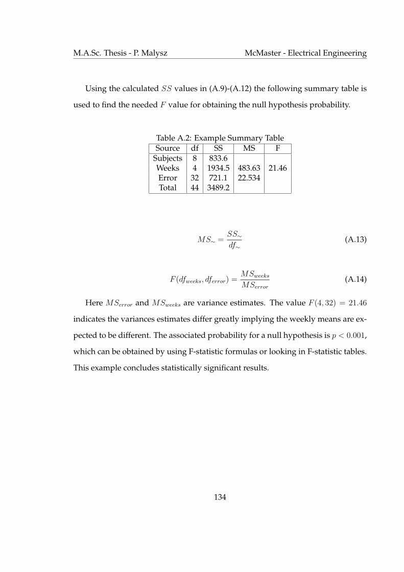
M.A.Sc. Thesis - P. Malysz McMaster - Electrical Engineering
Using the calculated SS values in (A.9)-(A.12) the following summary table is
used to find the needed F value for obtaining the null hypothesis probability.
Table A.2: Example Summary TableSource df SS MS F
Subjects 8 833.6Weeks 4 1934.5 483.63 21.46Error 32 721.1 22.534Total 44 3489.2
MS∼ =SS∼df∼
(A.13)
F (dfweeks, dferror) =MSweeks
MSerror
(A.14)
Here MSerror and MSweeks are variance estimates. The value F (4, 32) = 21.46
indicates the variances estimates differ greatly implying the weekly means are ex-
pected to be different. The associated probability for a null hypothesis is p < 0.001,
which can be obtained by using F-statistic formulas or looking in F-statistic tables.
This example concludes statistically significant results.
134

Bibliography
[1] K. Hashtrudi-zaad and S. Salcudean, “Analysis of control architectures for
teleoperation systems with impedance/admittance master and slave manip-
ulators,” Int. J. Robot. Res., vol. 20, no. 6, pp. 419–445, 2001.
[2] N. Tan and D. P. Atherton, “Frequency response of uncertain systems: A 2q-
convex parpolygonal approach,” IEE Proc. Control Theory Appl., vol. 147, no. 5,
pp. 547–555, 2000.
[3] C. V. Hollot and R. Temp, “On the nyquist envelope of an interval plant fam-
ily,” IEEE Tran. Automat. Cont., vol. 39, no. 2, pp. 391–396, 1994.
[4] G. Gescheider, Psychophysics The Fundamentals. Mahwah NJ: Lawrence Erl-
baum Associates, 1997.
[5] K. S. Hale and K. M. Stanney, “Deriving haptic guidelines from human physi-
ological, psychophysical, and neurological foundations,” IEEE Comp Graphics
and Applications, vol. 24, no. 2, pp. 33–39, 2004.
[6] P. F. Hokayem and M. W. Spong, “Bilateral teleoperation: an historical sur-
vey,” Automatica, pp. 2035–2057, 2006.
135
M.A.Sc. Thesis - P. Malysz McMaster - Electrical Engineering
[7] S. Salcudean, Control for Teleoperation and Haptic Interfaces. Control Problems
in Robotics and Automation; B. Siciliano and K.P. Valavanis (Eds.), Springer,
1997.
[8] P. Dario, B. Hannaford, and A. Menciassi, “Smart surgical tools and augment-
ing devices,” IEEE trans on Robotics and Automation, vol. 19, no. 5, pp. 782–792,
2003.
[9] G. D. Gersem, H. V. Brussel, and F. Tendick, “Reliable and enhanced stiff-
ness perception in soft-tissue telemanipulation,” Int. J. Robot. Research, vol. 24,
no. 10, pp. 805–822, 2005.
[10] M. Cavusoglu, A. Sherman, and F. Tendick, “Design of bilateral teleoperation
controllers for haptic exploration and telemanipulation of soft environments,”
IEEE Trans. Robot. Automat., vol. 18, no. 4, pp. 641–647, 2002.
[11] B. Hannaford, “A design framework for teleoperators with kinesthetic feed-
back,” IEEE Trans. Robot. Automat., vol. 5, pp. 426–434, August 1989.
[12] D. Lawrence, “Stability and transparency in bilateral teleoperation,” IEEE
Trans. Robot. Automat., vol. 9, pp. 624–637, October 1993.
[13] G. Raju, G. Verghese, and T. Sheridan, “Design issues in 2-port network mod-
els of bilateral remote teleoperation,” in Proc. IEEE Int. Conf. Robot. Automat.,
pp. 1317–1321, 1989.
[14] H. Kazerooni, T. Tsay, and K. Hollerbach, “A controller design framework for
telerobotic systems,” IEEE Trans. Contr. Syst. Technol., vol. 1, pp. 50–62, March
1993.
136

M.A.Sc. Thesis - P. Malysz McMaster - Electrical Engineering
[15] G. Leung, B. Francis, and J. Apkarian, “Bilateral controller for teleoperators
with time delay via mu-synthesis,” IEEE Trans. Robot. Automat., vol. 11, no. 1,
pp. 105–116, 1995.
[16] Y. Yokokohji and T. Yoshikawa, “Bilateral control of master-slave manipula-
tors for ideal kinesthetic coupling-formulation and experiment,” IEEE Trans.
Robot. Automat., vol. 10, pp. 605–620, October 1994.
[17] G. Niemeyer and J.-J. Slotine, “Stable adpative teleoperation,” IEEE J. Oceanic
Eng., vol. 16, no. 1, pp. 152–162, 1991.
[18] Y. Yokokohji, T. Imaida, and T. Yoshikawa, “Bilateral control with energy bal-
ance monitoring under time-varying communication delay,” in Proc. IEEE Int.
Conf. Robot. Automat., pp. 2684–2689, 2000.
[19] K. Hashtrudi-Zaad and S. Salcudean, “Transparency in time-delayed systems
and the effect of local force feedback for transparent teleoperation,” IEEE
Trans. Robot. Automat., vol. 18, no. 1, pp. 108–114, 2002.
[20] S. Sirouspour and A. Shahdi, “Discrete-time linear quadratic gaussian control
for teleoperation under communication time delay,” The Int. Journal of Robotics
Research, vol. 25, pp. 187–202, February 2006.
[21] S. Sirouspour and A. Shahdi, “Model predictive control for transparent tele-
operation under communication time delay,” IEEE trans on Robotics, pp. 1131–
1145, 2006.
137
M.A.Sc. Thesis - P. Malysz McMaster - Electrical Engineering
[22] A. Shahdi and S. Sirouspour, “Adaptive/robust control for enhanced teleop-
eration under communication time delay,” in Proceedings of IEEE conf. on In-
telligent Robots and Systems, Oct 2007.
[23] A. Shahdi and S. Sirouspour, “A multi-model decentralized controller for tele-
operation with time delay,” in Proceedings of IEEE conf. on Intelligent Robots and
Systems, Oct 2007.
[24] J. Colgate, “Robust impedance shaping telemanipulation,” IEEE Trans. Robot.
Automat., vol. 9, pp. 374–384, August 1993.
[25] S. Sirouspour, “Modeling and control of cooperative teleoperation systems,”
IEEE Transactions on Robotics, vol. 21, pp. 1220–1225, December 2005.
[26] W. Zhu and S. Salcudean, “Stability guaranteed teleoperation: an adap-
tive motion/force control approach,” IEEE Trans. Automat. Contr., vol. 45,
pp. 1951–1969, November 2000.
[27] J.-E. Slotine and W. Li, Applied Nonlinear Control. New Jersey: Prentice-Hall
Inc., 1991.
[28] L. Sciavicco and B. Siciliano, Modeling and Control of Robot Manipulators, Second
Edition. Springer-Verlag, 2000.
[29] J. O. Perreault and C. G. L. Cao, “Effects of vision and friction on haptic per-
ception,” Human Factors, vol. 48, no. 3, pp. 574–586, 2006.
[30] M. Tavakoli, R. V. Patel, and M. Moallem, “Haptic interaction in robot-assisted
endoscopic surgery: a sensorized end-effector,” Int. J. Medical Robotics and
CAS, vol. 1, no. 2, pp. 53–63, 2005.
138
M.A.Sc. Thesis - P. Malysz McMaster - Electrical Engineering
[31] B. Deml, T. Ortmaier, and U. Seibold, “The touch and feel in minimally inva-
sive surgery,” in Proceedings of IEEE Int. Workshop Haptic Audio Visual Envir.
and Applic., pp. 33–38, Oct 2005.
[32] L. Zamorano, Q. Li, S. Jain, and G. Kaur, “Robotics in neurosurgery: state of
the art and future technological challenges,” Int. J. Medical Robotics and CAS,
vol. 1, no. 1, pp. 7–22, 2004.
[33] A. Rossi, A. Trevisani, and V. Zanotto, “A telerobotic haptic system for min-
imally invasive stereotactic neurosurgery,” Int. J. Medical Robotics and CAS,
vol. 1, no. 2, pp. 64–75, 2005.
[34] C. N. Riviere, R. S. Rader, and P. K. Khosla, “Characteristics of hand motion
of eye surgeons,” in Proc. Int. Conf. IEEE/EMBS, pp. 1690–1693, 1997.
[35] C. N. Riviere and N. V. Thakor, “Suppressing pathological tremor during dex-
trous teleoperation,” in Proceedings of IEEE Engineering in Medicine and Biology,
pp. 1195–1196, Sept 1995.
[36] A. M. Okamura, “Methods for haptic feedback in teleoperated robot-assisted
surgery,” Industrial Robot: An international journal, vol. 31, no. 6, pp. 499–508,
2004.
[37] X. Wang, P. X. Liu, B. Chebbi, D. Wang, and M. Meng, “Design of bilateral
teleoperators for soft environments with adaptive environmental impedance
estimation,” in Proc. IEEE Int. Conf. Robotics Automation, pp. 1127–1132, 2005.
[38] R. H. Lamotte, “Softness discrimination with a tool,” Journal of Neurophysiol-
ogy, pp. 1777–1786, 2000.
139

M.A.Sc. Thesis - P. Malysz McMaster - Electrical Engineering
[39] M. K. O’malley and M. Goldfarb, “Comparison of human size identification
and discrimination performance in real and simulated environments,” in Pro-
ceedings of IEEE Symp on Haptic interfaces for Virt. Envir. and Teleoperator systs.,
pp. 10–17, Mar 2002.
[40] M. K. O’malley and M. Goldfarb, “The implications of surface stiffness for size
identification and perceived surface hardness in haptic interfaces,” in Proceed-
ings of IEEE conf. on Robotics and Automation, pp. 1255–1260, May 2002.
[41] M. K. O’malley and M. Goldfarb, “The effect of force saturation on the haptic
perception of detail,” IEEE/ASME trans on mechatronics, pp. 280–288, 2002.
[42] M. K. O’malley and M. Goldfarb, “The effect of virtual surface stiffness on the
haptic perception of detail,” IEEE/ASME trans on mechatronics, pp. 448–454,
2004.
[43] G. D. Gersem, H. V. Brussel, and F. Tendick, “A new optimization function for
force feedback in teleoperation,” in Proc. Int. Conf. Computer Assisted Radiology
and Surgery, p. 1354, 2003.
[44] W. Wu, C. Basdogan, and M. A. Srinivasan, “Visual, haptic, and bimodal per-
ception of size and stiffness in virtual environments,” in Proc. ASME Dynamic
Systems and Control Division, pp. 19–26, 1999.
[45] M. A. Srinivasan, G. L. Beauregard, and D. L. Brock, “The impact of visual
information on the haptic perception of stiffness in virtual environments,” in
Proc. ASME Dynamic Systems and Control Division, pp. 555–559, 1996.
140
M.A.Sc. Thesis - P. Malysz McMaster - Electrical Engineering
[46] F. Barbagli, K. Salisbury, C. Ho, C. Spence, and H. Tan, “Haptic discrimination
of force direction and the influence of visual information,” ACM Trans. Applied
Perception, vol. 3, no. 2, pp. 125–135, 2006.
[47] V. L. Kharitonov, “Asymptotic stability of an equilibrium position of a fam-
ily of systems of linear differential equations,” Differential Equations, vol. 14,
pp. 1483–1485, 1979.
[48] S. P. Bhattacharyya, H. Chapellat, and L. H. Keel, Robust Control: the parametric
approach. Prentice Hall, 1995.
[49] B. R. Barmish, “A generalization of kharitonov four-polynomial concept for
robust stability problems with linearly dependent coefficient perturbations,”
IEEE Trans. Automatic Control, vol. 34, no. 2, pp. 157–165, 1989.
[50] S. Boyd and L. Vandenberghe, Convex Optimization. Cambridge: Cambridge
University Press, 2004.
[51] A. Barlett, C. V. Hollot, and H. Lin, “Root location of an entire polytope of
polynomials: it sufficies to check the edges,” Math. Control, Signals. Syst., no. 1,
pp. 61–71, 1988.
[52] N. Tan, “Robust phase margin, robust gain margin and nyquist envelope of
an interval plant family,” Computers and Electrical Engineering, vol. 30, no. 2,
pp. 153–165, 2004.
[53] A. I. Lur’e and V. N. Postnikov, “On the theory of stability of control systems,”
Applied mathematics and mechanics, vol. 8, no. 3, 1944.
141

M.A.Sc. Thesis - P. Malysz McMaster - Electrical Engineering
[54] A. van der Schaft, L2-Gain and Passivity Techniques in Nonlinear Control 2nd Ed.
London: Springer-Verlag, 2000.
[55] M. Vidyasagar, Nonlinear Systems Analysis. Englewood Cliffs NJ: Prentice Hall,
1993.
[56] G. Zames, “On the input-output stability of time-varying nonlinear feedback
systems-part i: conditions derived using concepts of loop gain, conicity, and
positivity,” IEEE Trans. Automatic Control, no. 2, pp. 228–238, 1966.
[57] G. Zames, “On the input-output stability of time-varying nonlinear feedback
systems-part ii: conditions involving circles in the frequency plane and sector
nonlinearites,” IEEE Trans. Automatic Control, no. 3, pp. 465–476, 1966.
[58] Y.-S. Cho and K. S. Narendra, “An off-axis circle criterion for the stability of
feedback systems with a monotonic nonlinearity,” IEEE Tran. Automat. Cont.,
vol. 13, no. 4, pp. 413–416, 1968.
[59] M. S. Ghausi and J. J. Kelly, Introduction to Distributed-Parameter Networks with
Application to Integrated Circuits. New York: Holt, Rinehart and Winston Inc.,
1968.
[60] V. V. Kulkarni and M. G. Safonov, “Incremental positivity nonpreservation by
stability multipliers,” IEEE Trans. Automatic Control, vol. 47, no. 1, 2002.
[61] K. S. Narendra and Y. S. Cho, “Stability of feedback systems containing a sin-
gle odd monotonic nonlinearity,” IEEE Trans Automatic Control, vol. 12, no. 4,
pp. 448–450, 1967.
142

M.A.Sc. Thesis - P. Malysz McMaster - Electrical Engineering
[62] D. Materassi, M. Salapaka, and B. Basso, “A less conservative circle criterion,”
in Proceedings of the American Control Conf., pp. 824–827, June 2006.
[63] T. Mori, T. Nishimura, Y. Kuroe, and H. Kokame, “Off-axis circle criteria for
lur’e systems with interval plants,” in Proceedings of IEEE conf. on Decision and
Control, pp. 585–586, Dec 1994.
[64] N. Tan and D. P. Atherton, “New approach to assessing the effects of para-
metric variations in feedback loops,” IEE Proc. Control Theory Appl., vol. 150,
no. 2, pp. 101–111, 2003.
[65] S. S. Stevens, “On the pyschophysical law,” Psychological Review, pp. 153–181,
1957.
[66] H. Levitt, “Transformed up-down methods in psychoacoustics,” J. Acoustical
Society of America, vol. 49, pp. 467–477, 1970.
[67] G. Bekesy, “A new audiometer,” Acta Oto-laryngology, pp. 411–422, 1947.
[68] L. G. Brown, “Additional rules for the transformed up-down method in psy-
chophysics,” Perception and Psychophysics, pp. 959–962, 1996.
[69] C. Kaernbach, “Simple adaptive testing with the weighted up-down
method,” Perception and Psychophysics, vol. 49, pp. 227–229, 1991.
[70] T. H. Rammsayer, “An experimental comparison of the weighted up-down
method and transformed up-down method,” Bulletin of the Psychonomic Soci-
ety, pp. 425–427, 1992.
143

M.A.Sc. Thesis - P. Malysz McMaster - Electrical Engineering
[71] D. Howell, Fundamental Statistics for the Behavioral Sciences 5th Ed. Belmont
CA: Brooks/Cole, 2004.
144