Engle (2004)

American Economic Association

Risk and Volatility: Econometric Models and Financial PracticeAuthor(s): Robert EngleSource: The American Economic Review, Vol. 94, No. 3 (Jun., 2004), pp. 405-420Published by: American Economic AssociationStable URL: http://www.jstor.org/stable/3592935 .

Accessed: 02/04/2013 12:00

Your use of the JSTOR archive indicates your acceptance of the Terms & Conditions of Use, available at .http://www.jstor.org/page/info/about/policies/terms.jsp

.JSTOR is a not-for-profit service that helps scholars, researchers, and students discover, use, and build upon a wide range ofcontent in a trusted digital archive. We use information technology and tools to increase productivity and facilitate new formsof scholarship. For more information about JSTOR, please contact [email protected].

.

American Economic Association is collaborating with JSTOR to digitize, preserve and extend access to TheAmerican Economic Review.

http://www.jstor.org

This content downloaded from 200.37.165.17 on Tue, 2 Apr 2013 12:00:10 PMAll use subject to JSTOR Terms and Conditions

http://www.jstor.org/action/showPublisher?publisherCode=aea

http://www.jstor.org/stable/3592935?origin=JSTOR-pdf

http://www.jstor.org/page/info/about/policies/terms.jsp


Risk and Volatility: Econometric Models and Financial Practicet

By ROBERT ENGLE*

The advantage of knowing about risks is that we can change our behavior to avoid them. Of course, it is easily observed that to avoid all risks would be impossible; it might entail no flying, no driving, no walking, eating and drink- ing only healthy foods, and never being touched by sunshine. Even a bath could be dangerous. I could not receive this prize if I sought to avoid all risks. There are some risks we choose to take because the benefits from taking them exceed the possible costs. Optimal behavior takes risks that are worthwhile. This is the central para- digm of finance; we must take risks to achieve rewards but not all risks are equally rewarded. Both the risks and the rewards are in the future, so it is the expectation of loss that is balanced against the expectation of reward. Thus we op- timize our behavior, and in particular our portfolio, to maximize rewards and minimize risks.

This simple concept has a long history in economics and in Nobel citations. Harry M. Markowitz (1952) and James Tobin (1958) as- sociated risk with the variance in the value of a portfolio. From the avoidance of risk they de- rived optimizing portfolio and banking behavior. William Sharpe (1964) developed the implications when all investors follow the same objectives with the same information. This theory is called the Capital Asset Pricing Model or CAPM, and shows that there is a natural rela-

t This article is a revised version of the lecture Robert Engle delivered in Stockholm, Sweden, on December 8, 2003, when he received the Bank of Sweden Prize in Eco- nomic Sciences in Memory of Alfred Nobel. The article is copyright ? The Nobel Foundation 2003 and is published here with the permission of the Nobel Foundation.

* Stern School of Business, New York University, 44 West Fourth Street, New York, NY 10012 (e-mail: [email protected]). This paper is the result of more than two decades of research and collaboration with many, many people. I would particularly like to thank the audiences in B.I.S., Stockholm, Uppsala, Cornell University, and the Universite de Savoie for listening as this talk developed. David Hendry, Tim Bollerslev, Andrew Patton, and Robert Ferstenberg provided detailed suggestions. Nevertheless, any lacunas remain my responsibility.

tion between expected returns and variance. These contributions were recognized by Nobel prizes in 1981 and 1990.

Fisher Black and Myron Scholes (1972) and Robert C. Merton (1973) developed a model to evaluate the pricing of options. While the theory is based on option replication arguments through dynamic trading strategies, it is also consistent with the CAPM. Put options give the owner the right to sell an asset at a particular price at a time in the future. Thus these options can be thought of as insurance. By purchasing such put options, the risk of the portfolio can be

completely eliminated. But what does this insurance cost? The price of protection depends upon the risks and these risks are measured by the variance of the asset returns. This contribu- tion was recognized by a 1997 Nobel prize.

When practitioners implemented these financial strategies, they required estimates of the variances. Typically the square root of the variance, called the volatility, was reported. They immediately recognized that the volatilities were changing over time. They found different answers for different time periods. A simple approach, sometimes called historical volatility, was, and remains, widely used. In this method, the volatility is estimated by the sample standard deviation of returns over a short period. But, what is the right period to use? If it is too long, then it will not be so relevant for today and if it is too short, it will be very noisy. Furthermore, it is really the volatility over a future period that should be considered the risk, hence a forecast of volatility is needed as well as a measure for today. This raises the possibil- ity that the forecast of the average volatility over the next week might be different from the forecast over a year or a decade. Historical volatility had no solution for these problems.

On a more fundamental level, it is logically inconsistent to assume, for example, that the variance is constant for a period such as one year ending today and also that it is constant for the year ending on the previous day but with a different value. A theory of dynamic volatilities

405



THE AMERICAN ECONOMIC REVIEW

is needed; this is the role that is filled by the ARCH models and their many extensions that we discuss today.

In the next section, I will describe the genesis of the ARCH model, and then discuss some of its many generalizations and widespread empirical support. In subsequent sections, I will show how this dynamic model can be used to forecast volatility and risk over a long horizon and how it can be used to value options.

I. The Birth of the ARCH Model

The ARCH model was invented while I was on sabbatical at the London School of Econom- ics in 1979. Lunch in the Senior Common Room with David Hendry, Dennis Sargan, Jim Durbin, and many leading econometricians provided a stimulating environment. I was looking for a model that could assess the validity of a conjecture of Milton Friedman (1977) that the unpredictability of inflation was a primary cause of business cycles. He hypothesized that the level of inflation was not a problem; it was the uncertainty about future costs and prices that would prevent entrepreneurs from investing and lead to a recession. This could only be plausible if the uncertainty were changing over time so this was my goal. Econometricians call this heteroskedasticity. I had recently worked exten- sively with the Kalman Filter and knew that a likelihood function could be decomposed into the sum of its predictive or conditional densi- ties. Finally, my colleague, Clive Granger, with whom I share this prize, had recently developed a test for bilinear time series models based on the dependence over time of squared residuals. That is, squared residuals often were autocorre- lated even though the residuals themselves were not. This test was frequently significant in economic data; I suspected that it was detecting something besides bilinearity but I did not know what.

The solution was autoregressive conditional heteroskedasticity or ARCH, a name invented by David Hendry. The ARCH model described the forecast variance in terms of current observables. Instead of using short or long sample standard deviations, the ARCH model proposed taking weighted averages of past squared forecast errors, a type of weighted variance. These weights could give more influence to recent

information and less to the distant past. Clearly the ARCH model was a simple generalization of the sample variance.

The big advance was that the weights could be estimated from historical data even though the true volatility was never observed. Here is how this works. Forecasts can be calculated every day or every period. By examining these forecasts for different weights, the set of weights can be found that make the forecasts closest to the variance of the next return. This procedure, based on Maximum Likelihood, gives a systematic approach to the estimation of the optimal weights. Once the weights are determined, this dynamic model of time-varying volatility can be used to measure the volatility at any time and to forecast it into the near and distant future. Granger's test for bilinearity turned out to be the optimal, or Lagrange Mul- tiplier test for ARCH, and is widely used today.

There are many benefits to formulating an explicit dynamic model of volatility. As mentioned above, the optimal parameters can be estimated by Maximum Likelihood. Tests of the adequacy and accuracy of a volatility model can be used to verify the procedure. One-step and multi-step forecasts can be constructed using these parameters. The unconditional distributions can be established mathematically and are generally realistic. Inserting the relevant variables into the model can test economic models that seek to determine the causes of volatility. Incorporating additional endogenous variables and equations can similarly test economic models about the consequences of volatility. Several applications will be mentioned below.

David Hendry's associate, Frank Srba, wrote the first ARCH program. The application that appeared in Engle (1982) was to inflation in the United Kingdom since this was Friedman's conjecture. While there was plenty of evidence that the uncertainty in inflation forecasts was time varying, it did not correspond to the U.K. business cycle. Similar tests for U.S. inflation data, reported in Engle (1983), confirmed the finding of ARCH but found no business-cycle effect. While the trade-off between risk and return is an important part of macroeconomic theory, the empirical implications are often difficult to detect as they are disguised by other dominating effects, and obscured by the reli- ance on relatively low-frequency data. In fi-

JUNE 2004 406



ENGLE: RISK AND VOLATILITY

nance, the risk/return effects are of primary importance and data on daily or even intradaily frequencies are readily available to form accurate volatility forecasts. Thus finance is the field in which the great richness and variety of ARCH models developed.

II. Generalizing the ARCH Model

Generalizations to different weighting schemes can be estimated and tested. The very important development by my outstanding student Tim Bollerslev (1986), called Generalized Autoregressive Conditional Heteroskedasticity, or GARCH, is today the most widely used model. This essentially generalizes the purely autoregressive ARCH model to an autoregressive moving average model. The weights on past squared residuals are assumed to decline geometrically at a rate to be estimated from the data. An intuitively appealing interpretation of the GARCH(1,1) model is easy to understand. The GARCH forecast variance is a weighted average of three different variance forecasts. One is a constant variance that corresponds to the long-run average. The second is the forecast that was made in the previous period. The third is the new information that was not available when the previous forecast was made. This could be viewed as a variance forecast based on one period of information. The weights on these three forecasts determine how fast the variance changes with new information and how fast it reverts to its long-run mean.

A second enormously important generalization was the Exponential GARCH or EGARCH model of Daniel B. Nelson (1991), who prema- turely passed away in 1995 to the great loss of our profession as eulogized by Bollerslev and Peter E. Rossi (1995). In his short academic career, his contributions were extremely influ- ential. He recognized that volatility could re- spond asymmetrically to past forecast errors. In a financial context, negative returns seemed to be more important predictors of volatility than positive returns. Large price declines forecast greater volatility than similarly large price increases. This is an economically interesting effect that has wide-ranging implications to be discussed below.

Further generalizations have been proposed by many researchers. There is now an alphabet

soup of ARCH models that include: AARCH, APARCH, FIGARCH, FIEGARCH, STARCH, SWARCH, GJR-GARCH, TARCH, MARCH, NARCH, SNPARCH, SPARCH, SQGARCH, CESGARCH, Component ARCH, Asymmetric Component ARCH, Taylor-Schwert, Student-t- ARCH, GED-ARCH, and many others that I have regrettably overlooked. Many of these models were surveyed in Bollerslev et al. (1992), Bollerslev et al. (1994), Engle (2002b), and Engle and Isao Ishida (2002). These models recognize that there may be important nonlin- earity, asymmetry, and long memory properties of volatility and that returns can be nonnormal with a variety of parametric and nonparametric distributions.

A closely related but econometrically distinct class of volatility models called Stochastic Vol- atility, or SV models, have also seen dramatic development. See, for example, Peter K. Clark (1973), Stephen Taylor (1986), Andrew C. Har-

vey et al. (1994), and Taylor (1994). These models have a different data-generating process which makes them more convenient for some

purposes but more difficult to estimate. In a linear framework, these models would simply be different representations of the same process; but in this nonlinear setting, the alternative specifications are not equivalent, although they are close approximations.

III. Modeling Financial Returns

The success of the ARCH family of models is attributable in large measure to the applications in finance. While the models have applicability for many statistical problems with time series data, they find particular value for financial time series. This is partly because of the importance of the previously discussed trade-off between risk and return for financial markets, and partly because of three ubiquitous characteristics of financial returns from holding a risky asset. Returns are almost unpredictable, they have sur- prisingly large numbers of extreme values, and both the extremes and quiet periods are clustered in time. These features are often described as unpredictability, fat tails, and volatility clustering. These are precisely the characteristics for which an ARCH model is designed. When volatility is high, it is likely to remain high, and when it is low, it is likely to remain low. However,

407 VOL. 94 NO. 3




these periods are time limited so that the forecast is sure to eventually revert to less extreme volatilities. An ARCH process produces dynamic, mean-reverting patterns in volatility that can be forecast. It also produces a greater number of extremes than would be expected from a standard normal distribution, since the extreme values during the high volatility period are greater than could be anticipated from a constant volatility process.

The GARCH(1,1) specification is the work- horse of financial applications. It is remarkable that one model can be used to describe the volatility dynamics of almost any financial return series. This applies not only to U.S. stocks but also to stocks traded in most developed markets, to most stocks traded in emerging markets, and to most indices of equity returns. It applies to exchange rates, bond returns, and commodity returns. In many cases, a slightly better model can be found in the list of models above, but GARCH is generally a very good starting point.

The widespread success of GARCH(1,1) begs to be understood. What theory can explain why volatility dynamics are similar in so many different financial markets? In developing such a theory, we must first understand why asset prices change. Financial assets are purchased and owned because of the future payments that can be expected. Because these payments are uncertain and depend upon unknowable future developments, the fair price of the asset will require forecasts of the distribution of these payments based on our best information today. As time goes by, we get more information on these future events and revalue the asset. So at a basic level, financial price volatility is due to the arrival of new information. Volatility clustering is simply clustering of information arriv- als. The fact that this is common to so many assets is simply a statement that news is typically clustered in time.

To see why it is natural for news to be clustered in time, we must be more specific about the information flow. Consider an event such as an invention that will increase the value of a firm because it will improve future earnings and dividends. The effect on stock prices of this event will depend on economic conditions in the economy and in the firm. If the firm is near bankruptcy, the effect can be very large and if it is already operating at full capacity, it may be

small. If the economy has low interest rates and surplus labor, it may be easy to develop this new product. With everything else equal, the response will be greater in a recession than in a boom period. Hence we are not surprised to find higher volatility in economic downturns even if the arrival rate of new inventions is constant. This is a slow moving type of volatility clustering that can give cycles of several years or longer.

The same invention will also give rise to a high-frequency volatility clustering. When the invention is announced, the market will not immediately be able to estimate its value on the stock price. Agents may disagree but be sufficiently unsure of their valuations that they pay attention to how others value the firm. If an investor buys until the price reaches his estimate of the new value, he may revise his estimate after he sees others continue to buy at succes- sively higher prices. He may suspect they have better information or models and consequently raise his valuation. Of course, if the others are selling, then he may revise his price downward. This process is generally called price discovery and has been modeled theoretically and empir- ically in market microstructure. It leads to volatility clustering at a much higher frequency than we have seen before. This process could last a few days or a few minutes.

But to understand volatility we must think of more than one invention. While the arrival rate of inventions may not have clear patterns, other types of news surely do. The news intensity is generally high during wars and economic distress. During important global summits, congressional or regulatory hearings, elections, or central bank board meetings, there are likely to be many news events. These episodes are likely to be of medium duration, lasting weeks or months.

The empirical volatility patterns we observe are composed of all three of these types of events. Thus we expect to see rather elaborate volatility dynamics and often rely on long time series to give accurate models of the different time constants.

IV. Modeling the Causes and Consequences of Financial Volatility

Once a model has been developed to measure volatility, it is natural to attempt to explain the

408 JUNE 2004




causes of volatility and the effects of volatility on the economy. There is now a large literature examining aspects of these questions. I will only give a discussion of some of the more limited findings for financial markets.

In financial markets, the consequences of volatility are easy to describe although perhaps difficult to measure. In an economy with one risky asset, a rise in volatility should lead investors to sell some of the asset. If there is a fixed supply, the price must fall sufficiently so that buyers take the other side. At this new lower price, the expected return is higher by just enough to compensate investors for the in- creased risk. In equilibrium, high volatility should correspond to high expected returns. Merton (1980) formulated this theoretical model in continuous time, and Engle et al. (1987) proposed a discrete time model. If the price of risk were constant over time, then rising conditional variances would translate linearly into rising expected returns. Thus the mean of the return equation would no longer be estimated as zero, it would depend upon the past squared returns exactly in the same way that the conditional variance depends on past squared returns. This very strong coefficient restriction can be tested and used to estimate the price of risk. It can also be used to measure the coefficient of relative risk aversion of the representa- tive agent under the same assumptions.

Empirical evidence on this measurement has been mixed. While Engle et al. (1987) find a positive and significant effect, Ray-Yeutien Chou et al. (1992) and Lawrence R. Glosten et al. (1993) find a relationship that varies over time and may be negative because of omitted variables. Kenneth R. French et al. (1987) showed that a positive volatility surprise should and does have a negative effect on asset prices. There is not simply one risky asset in the economy and the price of risk is not likely to be constant; hence the instability is not surprising and does not disprove the existence of the risk return trade-off, but it is a challenge to better modeling of this trade-off.

The causes of volatility are more directly modeled. Since the basic ARCH model and its many variants describe the conditional variance as a function of lagged squared returns, these are perhaps the proximate causes of volatility. It is best to interpret these as observables that help

in forecasting volatility rather than as causes. If the true causes were included in the specification, then the lags would not be needed.

A small collection of papers has followed this route. Torben G. Andersen and Bollerslev (1998b) examined the effects of announcements on exchange rate volatility. The difficulty in finding important explanatory power is clear even if these announcements are responsible in

important ways. Another approach is to use the volatility measured in other markets. Engle et al. (1990b) find evidence that stock volatility causes bond volatility in the future. Engle et al. (1990a) model the influence of volatility in markets with earlier closing on markets with later closing. For example, they examine the influence of currency volatilities in European, Asian markets, and the prior day U.S. market on today's U.S. currency volatility. Yasushi Hamao et al. (1990), Pat Bums et al. (1998), and others have applied similar techniques to global equity markets.

V. An Example

To illustrate the use of ARCH models for financial applications, I will give a rather extended analysis of the Standard & Poors 500 Composite index. This index represents the bulk of the value in the U.S. equity market. I will look at daily levels of this index from 1963 through late November 2003. This gives a

sweep of U.S. financial history that provides an ideal setting to discuss how ARCH models are used for risk management and option pricing. All the statistics and graphs are computed in EViewsTM 4.1.

The raw data are presented in Figure 1 where

prices are shown on the left axis. The rather smooth lower curve shows what has happened to this index over the last 40 years. It is easy to see the great growth of equity prices over the

period and the subsequent decline after the new millennium. At the beginning of 1963 the index was priced at $63 and at the end it was $1,035. That means that one dollar invested in 1963 would have become $16 by November 21, 2003

(plus the stream of dividends that would have been received, as this index does not take ac- count of dividends on a daily basis). If this investor were clever enough to sell his position on March 24, 2000, it would have been worth

409 VOL. 94 NO. 3




- SP500 SPRETURNS |

FIGURE 1. S&P 500 DAILY PRICES AND RETURNS FROM

JANUARY 1963 TO NOVEMBER 2003

$24. Hopefully he was not so unlucky as to have purchased on that day. Although we often see pictures of the level of these indices, it is obvi- ously the relative price from the purchase point to the sale point that matters. Thus economists focus attention on returns as shown at the top of the figure. This shows the daily price change on the right axis (computed as the logarithm of the price today divided by the price yesterday). This return series is centered around zero throughout the sample period even though prices are sometimes increasing and sometimes decreasing. Now the most dramatic event is the crash of October 1987 which dwarfs all other returns in the size of the decline and subsequent partial recovery.

Other important features of this data series can be seen best by looking at portions of the whole history. For example, Figure 2 shows the same graph before 1987. It is very apparent that the amplitude of the returns is changing. The magnitude of the changes is sometimes large and sometimes small. This is the effect that ARCH is designed to measure and that we have called volatility clustering. There is, however, another interesting feature in this graph. It is clear that the volatility is higher when prices are falling. Volatility tends to be higher in bear markets. This is the asymmetric volatility effect that Nelson described with his EGARCH model.

Looking at the next subperiod after the 1987 crash in Figure 3, we see the record low vola-

1,600-

800-

400-

200-

- SP500 - SPRETURNS I

FIGURE 2. S&P 500 DAILY BEFORE 1987

-0.04

-0.00

- 0.04

--0.08

1988 1990 1992 1994 1996 1998 2000

I - SP500 . SPRETURNS

FIGURE 3. S&P 500 1988 TO 2000

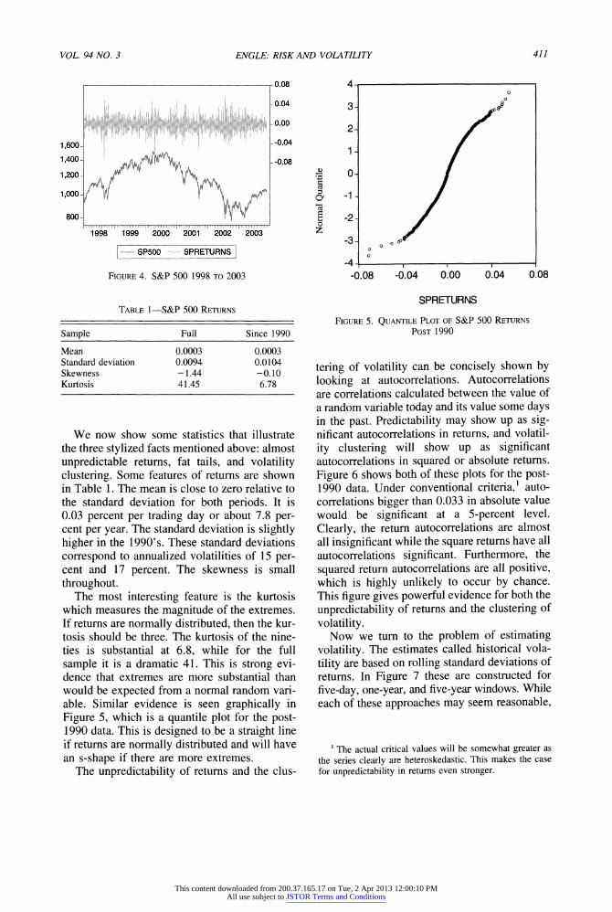
tility period of the middle 1990's. This was accompanied by a slow and steady growth of equity prices. It was frequently discussed whether we had moved permanently to a new era of low volatility. History shows that we did not. The volatility began to rise as stock prices got higher and higher, reaching very high levels from 1998 on. Clearly, the stock market was risky from this perspective but investors were willing to take this risk because the returns were so good. Looking at the last period since 1998 in Figure 4, we see the high volatility continue as the market turned down. Only at the end of the sample, since the official conclusion of the Iraq war, do we see substantial declines in volatility. This has apparently encouraged investors to come back into the market which has experienced substantial price increases.

u.ua

_ , } 4s I , ,

5 I ,

? , I . . .I

f l { r , I * X I . . . I * * . I J l I

JUNE 2004 410

n %f t

i.il: ii i I

,? ,:? I;;; i j 'i

t i




4

3-

2-

0

C

o 1998 1999 2000 2001 2002 2003

-- SP500 - SPRETURNS

FIGURE 4. S&P 500 1998 TO 2003

1-

0-

-1-

-2-

-3-

-4 ,

-0.08 -0.04 0.00 0.04 0.08

TABLE 1-S&P 500 RETURNS

Sample Full Since 1990

Mean 0.0003 0.0003 Standard deviation 0.0094 0.0104 Skewness -1.44 -0.10 Kurtosis 41.45 6.78

We now show some statistics that illustrate the three stylized facts mentioned above: almost unpredictable returns, fat tails, and volatility clustering. Some features of returns are shown in Table 1. The mean is close to zero relative to the standard deviation for both periods. It is 0.03 percent per trading day or about 7.8 percent per year. The standard deviation is slightly higher in the 1990's. These standard deviations correspond to annualized volatilities of 15 percent and 17 percent. The skewness is small throughout.

The most interesting feature is the kurtosis which measures the magnitude of the extremes. If returns are normally distributed, then the kurtosis should be three. The kurtosis of the nine- ties is substantial at 6.8, while for the full sample it is a dramatic 41. This is strong evidence that extremes are more substantial than would be expected from a normal random variable. Similar evidence is seen graphically in Figure 5, which is a quantile plot for the post- 1990 data. This is designed to be a straight line if returns are normally distributed and will have an s-shape if there are more extremes.

The unpredictability of returns and the clus-

SPRETURNS

FIGURE 5. QUANTILE PLOT OF S&P 500 RETURNS

POST 1990

tering of volatility can be concisely shown by looking at autocorrelations. Autocorrelations are correlations calculated between the value of a random variable today and its value some days in the past. Predictability may show up as significant autocorrelations in returns, and volatility clustering will show up as significant autocorrelations in squared or absolute returns. Figure 6 shows both of these plots for the post- 1990 data. Under conventional criteria,' autocorrelations bigger than 0.033 in absolute value would be significant at a 5-percent level. Clearly, the return autocorrelations are almost all insignificant while the square returns have all autocorrelations significant. Furthermore, the

squared return autocorrelations are all positive, which is highly unlikely to occur by chance. This figure gives powerful evidence for both the

unpredictability of returns and the clustering of volatility.

Now we turn to the problem of estimating volatility. The estimates called historical volatility are based on rolling standard deviations of returns. In Figure 7 these are constructed for five-day, one-year, and five-year windows. While each of these approaches may seem reasonable,

'The actual critical values will be somewhat greater as the series clearly are heteroskedastic. This makes the case for unpredictability in returns even stronger.

411 VOL. 94 NO. 3

A

o

0o o

A




l I ^ i i

, EI i .I I I

m SP Returns SQ Returns

FIGURE 6. RETURN AND SQUARED RETURN AUTOCORRELATIONS

1.6

1.2

0.8

0.4 i : 1 I;

I I I i '

p.: ,.,ja "

g - 'I

, .

. 65I

. I 70 75 80 85 90

I . . 95 65 70 75 80 85 90 95 X0

I .. V5 --- V260 --V1,3001

FIGURE 7. HISTORICAL VOLATILITIES WITH VARIOUS WINDOWS

the answers are clearly very different. The five- day estimate is extremely variable while the other two are much smoother. The five-year estimate smooths over peaks and troughs that the other two see. It is particularly slow to recover after the 1987 crash and particularly slow to reveal the rise in volatility in 1998- 2000. In just the same way, the annual estimate fails to show all the details revealed by the five-day volatility. However, some of these details may be just noise. Without any true measure of volatility, it is difficult to pick from these candidates.

The ARCH model provides a solution to this dilemma. From estimating the unknown param-

eters based on the historical data, we have forecasts for each day in the sample period and for any period after the sample. The natural first model to estimate is the GARCH(1,1). This model gives weights to the unconditional variance, the previous forecast, and the news measured as the square of yesterday's return. The weights are estimated to be (0.004, 0.941, 0.055), respectively.2 Clearly the bulk of the information comes from the previous day forecast. The new information changes this a little and the long-run average variance has a very small effect. It appears that the long-run variance effect is so tiny that it might not be important. This is incorrect. When forecasting many steps ahead, the long-run variance eventually dominates as the importance of news and other recent information fades away. It is natu- rally small because of the use of daily data.

In this example, we will use an asymmetric volatility model that is sometimes called GJR- GARCH for Glosten et al. (1993) or TARCH for Threshold ARCH (Jean Michael Zakoian, 1994). The statistical results are given in Table 2. In this case there are two types of news. There is a squared return and there is a variable that is the squared return when returns are negative, and zero otherwise. On average, this is

2 For a conventional GARCH model defined as ht+1 -I o + ar2 + P3ht, the weights are ((1 - a - 3), 3, a).

0.25

0.2

0.15

0.1

0.05

0

-0.05

-0.1

2.U

LU L x. . . . . . . . .. I . _' _ K , _' -. '

. . . . . . . . . . I t -w,

412 JUNE 2004




TABLE 2-TARCH ESTIMATES OF S&P 500 RETURN DATA

Dependent variable: NEWRET_SP Method: ML-ARCH (Marquardt) Date: 11/24/03 Time: 09:27 Sample (adjusted): 1/03/1963-11/21/2003 Included observations: 10,667 after adjusting endpoints Convergence achieved after 22 iterations Variance backcast: ON

C

C ARCH(1) (RESID < 0)*ARCH(1) GARCH(1)

Coefficient

0.000301

Variance equation

4.55E-07 0.028575 0.076169 0.930752

Standard error z-statistic Probability

6.67E-05 4.512504 0.0000

5.06E-08 0.003322 0.003821 0.002246

8.980473 8.602582 19.93374 414.4693

0.0000 0.0000 0.0000 0.0000

1.4

1.2 -

1.0 -

0.8-

0.6-

0.4-

0.2 -

0 .0 , , , . , , , . , , , 65 70 75 80 85 90 95 00

- GARCHVOL

FIGURE 8. GARCH VOLATILITIES

half as big as the variance, so it must be doubled implying that the weights are half as big. The weights are now computed on the long-run average, the previous forecast, the symmetric news, and the negative news. These weights are estimated to be (0.002, 0.931, 0.029, 0.038) respectively.3 Clearly the asymmetry is important since the last term would be zero otherwise. In fact, negative returns in this model have more than three times the effect of positive returns on future variances. From a statistical point of view, the asymmetry term has a t-statistic of almost 20 and is very significant.

The volatility series generated by this model is given in Figure 8. The series is more jagged

3 If the model is defined as ht = wo +- h_ + ar_ + -y t_It_l<0, then the weights are (1 - a - - y/2, 3, a, y/2).

0.10 ,,

1990 1992 1994 1996 198 2000 2002

|-- 3GARCHSTD - SPRETURNS ---3*GARCHSTD

FIGURE 9. GARCH CONFIDENCE INTERVALS: THREE STANDARD DEVIATIONS

than the annual or five-year historical volatilities, but is less variable than the five-day volatilities. Since it is designed to measure the volatility of returns on the next day, it is natural to form confidence intervals for returns. In Fig- ure 9 returns are plotted against plus and minus three TARCH standard deviations. Clearly the confidence intervals are changing in a very be- lievable fashion. A constant band would be too wide in some periods and too narrow in others. The TARCH intervals should have 99.7-percent probability of including the next observation if the data are really normally distributed. The expected number of times that the next return is outside the interval should then be only 29 out of the more than 10,000 days. In fact, there are 75 indicating that there are more outliers than would be expected from normality.

Additional information about volatility is available from the options market. The value of

413 VOL. 94 NO. 3




I VIX --GARCHM I

FIGURE 10. IMPLIED VOLATILITIES AND GARCH VOLATILITIES

traded options depends directly on the volatility of the underlying asset. A carefully constructed portfolio of options with different strikes will have a value that measures the option market estimate of future volatility under rather weak assumptions. This calculation is now performed by the CBOE for S&P 500 options and is reported as the VIX. Two assumptions that un- derlie this index are worth mentioning. The price process should be continuous and there should be no risk premia on volatility shocks. If these assumptions are good approximations, then implied volatilities can be compared with ARCH volatilities. Because the VIX represents the volatility of one-month options, the TARCH volatilities must be forecast out to one month.

The results are plotted in Figure 10. The general pattern is quite similar, although the TARCH is a little lower than the VIX. These differences can be attributed to two sources. First, the option pricing relation is not quite correct for this situation and does not allow for volatility risk premia or nonnormal returns. These adjustments would lead to higher options prices and consequently implied volatilities that were too high. Second, the basic ARCH models have very limited information sets. They do not use information on earnings, wars, elections, etc. Hence the volatility forecasts by traders should be generally superior; differences could be due to long-lasting information events.

This extended example illustrates many of the features of ARCH/GARCH models and how they can be used to study volatility processes. We turn now to financial practice and describe

two widely used applications. In the presentation, some novel implications of asymmetric volatility will be illustrated.

VI. Financial Practice-Value at Risk

Every morning in thousands of banks and financial services institutions around the world, the Chief Executive Officer is presented with a risk profile by his Risk Management Officer. He is given an estimate of the risk of the entire portfolio and the risk of many of its compo- nents. He would typically learn the risk faced by the firm's European Equity Division, its U.S. Treasury Bond Division, its Currency Trading Unit, its Equity Derivative Unit, and so forth. These risks may even be detailed for particular trading desks or traders. An overall figure is then reported to a regulatory body although it may not be the same number used for internal purposes. The risk of the company as a whole is less than the sum of its parts since different portions of the risk will not be perfectly correlated.

The typical measure of each of these risks is Value at Risk, often abbreviated as VaR. The VaR is a way of measuring the probability of losses that could occur to the portfolio. The 99-percent one-day VaR is a number of dollars that the manager is 99 percent certain will be worse than whatever loss occurs on the next day. If the one-day VaR for the currency desk is $50,000, then the risk officer asserts that only on one day out of 100 will losses on this portfolio be greater than $50,000. Of course this means that on about 2.5 days a year, the losses will exceed the VaR. The VaR is a measure of risk that is easy to understand without knowing any statistics. It is, however, just one quantile of the predictive distribution and therefore it has limited information on the probabilities of loss.

Sometimes the VaR is defined on a multi-day basis. A 99-percent ten-day VaR is a number of dollars that is greater than the realized loss over ten days on the portfolio with probability 0.99. This is a more common regulatory standard but is typically computed by simply adjusting the one-day VaR as will be discussed below. The loss figures assume that the portfolio is un- changed over the ten-day period which may be counterfactual.

414 JUNE 2004




To calculate the VaR of a trading unit or a firm as a whole, it is necessary to have variances and covariances, or equivalently volatilities and correlations, among all assets held in the portfolio. Typically, the assets are viewed as re- sponding primarily to one or more risk factors that are modeled directly. RiskmetricsTM, for example, uses about 400 global risk factors. BARRA uses industry risk factors as well as risk factors based on firm characteristics and other factors. A diversified U.S. equity portfolio would have risks determined primarily by the aggregate market index such as the S&P 500. We will carry forward the example of the previous section to calculate the VaR of a portfolio that mimics the S&P.

The one-day 99-percent VaR of the S&P can be estimated using ARCH. From historical data, the best model is estimated, and then the standard deviation is calculated for the following day. In the case of S&P on November 24, this forecast standard deviation is 0.0076. To con- vert this into VaR we must make an assumption about the distribution of returns. If normality is assumed, the 1 percent point is -2.33 standard deviations from zero. Thus the value at risk is 2.33 times the standard deviation or in the case of November 24, it is 1.77 percent. We can be 99 percent sure that we will not lose more than 1.77 percent of portfolio value on November 24. In fact the market went up on the 24th so there were no losses.

The assumption of normality is highly ques- tionable. We observed that financial returns have a surprising number of large returns. If we divide the returns by the TARCH standard deviations, the result will have a constant volatility of one but will have a nonnormal distribution. The kurtosis of these "devolatized returns," or "standardized residuals," is 6.5, which is much less than the unconditional kurtosis, but is still well above normal. From these devolatized returns, we can find the 1-percent quantile and use this to give a better idea of the VaR. It turns out to be 2.65 standard deviations below the mean. Thus our portfolio is riskier than we thought using the normal approxima- tion. The one-day 99-percent VaR is now estimated to be 2 percent.

A ten-day value at risk is often required by regulatory agencies and is frequently used internally as well. Of course, the amount a

portfolio can lose in ten days is a lot greater than it can lose in one day. But how much greater is it? If volatilities were constant, then the answer would be simple; it would be the square root of ten times as great. Since the ten-day variance is ten times the one-day variance, the ten-day volatility multiplier would be the square root of ten. We would take the one-day standard deviation and multiply it by 3.16 and then with normality we would multiply this by 2.33, giving 7.36 times the standard deviation. This is the conventional solution in industry practice. For November 24, the ten-day 99-percent VaR is 5.6 percent of portfolio value.

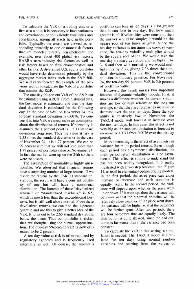
However, this result misses two important features of dynamic volatility models. First, it makes a difference whether the current volatilities are low or high relative to the long-run average, so that they are forecast to increase or decrease over the next ten days. Since the volatility is relatively low in November, the TARCH model will forecast an increase over the next ten days. In this case, this effect is not very big as the standard deviation is forecast to increase to 0.0077 from 0.0076 over the ten-day period.

More interesting is the effect of asymmetry in variance for multi-period returns. Even though each period has a symmetric distribution, the multi-period return distribution will be asymmetric. This effect is simple to understand but has not been widely recognized. It is easily illustrated with a two-step binomial tree, Figure 11, as used in elementary option pricing models. In the first period, the asset price can either increase or decrease and each outcome is

equally likely. In the second period, the variance will depend upon whether the price went

up or down. If it went up, then the variance will be lower so that the binomial branches will be relatively close together. If the price went down, the variance will be higher so that the outcomes will be further apart. After two periods, there are four outcomes that are equally likely. The distribution is quite skewed, since the bad outcome is far worse than if the variance had been constant.

To calculate the VaR in this setting, a simulation is needed. The TARCH model is simulated for ten days using normal random variables and starting from the values of

415 VOL. 94 NO. 3




Low variance

High variance

FIGURE 11. TWO-PERIOD BINOMIAL TREE WITH

ASYMMETRIC VOLATILITY

November 21.4 This was done 10,000 times and then the worst outcomes were sorted to find the Value at Risk corresponding to the 1-percent quantile. The answer was 7.89 times the standard deviation. This VaR is substantially larger than the value assuming constant volatility.

To avoid the normality assumption, the simulation can also be done using the empirical distribution of the standardized residuals. This simulation is often called a bootstrap; each draw of the random variables is equally likely to be any observation of the standardized residuals. The Oc- tober 1987 crash observation could be drawn once or even twice in some simulations but not in others. The result is a standard deviation multiplier of 8.52 that should be used to calculate VaR. For our case, the November 24 ten-day 99-percent VaR is 6.5 percent of portfolio value.

VII. Financial Practice-Valuing Options

Another important area of financial practice is valuation and management of derivatives

4 In the example here, the simulation was started at the unconditional variance so that the time aggregation effect could be examined alone. In addition, the mean was taken to be zero but this makes little difference over such short horizons.

such as options. These are typically valued theoretically assuming some particular process for the underlying asset and then market prices of the derivatives are used to infer the parameters of the underlying process. This strategy is often called "arbitrage free pricing." It is inadequate for some of the tasks of financial analysis. It cannot determine the risk of a derivative position since each new market price may correspond to a different set of parameters and it is the size and frequency of these parameter changes that signify risk. For the same reason, it is difficult to find optimal hedging strategies. Fi- nally, there is no way to determine the price of a new issue or to determine whether some derivatives are trading at discounts or premiums.

A companion analysis that is frequently car- ried out by derivatives traders is to develop fundamental pricing models that determine the appropriate price for a derivative based on the observed characteristics of the underlying asset. These models could include measures of trading cost, hedging cost, and risk in managing the options portfolio.

In this section, a simple simulation-based option pricing model will be employed to illustrate the use of ARCH models in this type of fundamental analysis. The example will be the pricing of put options on the S&P 500 that have ten trading days left to maturity.

A put option gives the owner the right to sell an asset at a particular price, called the strike price, at maturity. Thus if the asset price is below the strike, he can make money by selling at the strike and buying at the market price. The profit is the difference between these prices. If, however, the market price is above the strike, then there is no value in the option. If the investor holds the underlying asset in a portfolio and buys a put option, he is guaranteed to have at least the strike price at the maturity date. This is why these options can be thought of as insurance contracts.

The simulation works just as in the previous section. The TARCH model is simulated from the end of the sample period, 10,000 times. The bootstrap approach is taken so that nonnormal- ity is already incorporated in the simulation. This simulation should be of the "risk-neutral" distribution, i.e., the distribution in which assets are priced at their discounted expected values. The risk-neutral distribution differs from the

JUNE 2004 416




60

50- +

40- +

30- +

20 - + +

10-

O1 o 920 960 1,000 1,040

n 1 oQ

aL

Q.

1,080

K

FIGURE 12. PUT PRICES FROM GARCH SIMULATION

empirical distribution in subtle ways so that there is an explicit risk premium in the empirical distribution which is not needed in the risk neutral. In some models such as the Black- Scholes, it is sufficient to adjust the mean to be the risk-free rate. In the example, we take this route. The distribution is simulated with a mean of zero, which is taken to be the risk-free rate. As will be discussed below, this may not be a sufficient adjustment to risk-neutralize the distribution.

From the simulation, we have 10,000 equally likely outcomes for ten days in the future. For each of these outcomes we can compute the value of a particular put option. Since these are equally likely and since the riskless rate is taken to be zero, the fair value of the put option is the average of these values. This can be done for put options with different strikes. The result is plotted in Figure 12. The S&P is assumed to begin at 1,000 so a put option with a strike of 990 protects this value for ten days. This put option should sell for $11. To protect the portfolio at its current value would cost $15 and to be certain that it was at least worth 1,010 would cost $21. The VaR calculated in the previous section was $65 for the ten-day horizon. To protect the portfolio at this point would cost around $2. These put prices have the expected shape; they are monotonically increasing and convex.

However, these put prices are clearly differ-

0.164

0.160

0.15&

0.152

0.148

n 1AA

++

+4+

0 90 920 960 1,000 1,040 1,080

K

FIGURE 13. IMPLIED VOLATILITIES FROM GARCH SIMULATION

ent from those generated by the Black-Scholes model. This is easily seen by calculating the implied volatility for each of these put options. The result is shown in Figure 13. The implied volatilities are higher for the out-of-the-money puts than they are for the at-the-money puts; and the in-the-money put volatilities are even lower. If the put prices were generated by the Black- Scholes model, these implied volatilities would all be the same. This plot of implied volatilities against strike is a familiar feature for options traders. The downward slope is called a "volatility skew" and corresponds to a skewed distribution of the underlying assets. This feature is very pronounced for index options, less so for individual equity options, and virtually nonex- istent for currencies, where it is called a "smile." It is apparent that this is a consequence of the asymmetric volatility model and corre- spondingly, the asymmetry is not found for currencies and is weaker for individual equity options than for indices.

This feature of options prices is strong con- firmation of asymmetric volatility models. Un- fortunately, the story is more complicated than this. The actual options skew is generally somewhat steeper than that generated by asymmetric ARCH models. This calls into question the risk neutralization adopted in the simulation. There is now increasing evidence that investors are

F- a-

u. 10,;

U. I'l'. -- I

VOL. 94 NO. 3 417




particularly worried about big losses and are willing to pay extra premiums to avoid them. This makes the skew even steeper. The required risk neutralization has been studied by several authors such as Jens C. Jackwerth (2000), Joshua V. Rosenberg and Engle (2002), and David S. Bates (2003).

VIII. New Frontiers

It has now been more than 20 years since the ARCH paper appeared. The developments and applications have been fantastic and well be- yond anyone's most optimistic forecasts. But what can we expect in the future? What are the next frontiers?

There appear to be two important frontiers of research that are receiving a great deal of attention and have important promise for applications. These are high-frequency volatility models and high-dimension multivariate models. I will give a short description of some of the promising developments in these areas.

Merton was perhaps the first to point out the benefits of high-frequency data for volatility measurement. By examining the behavior of stock prices on a finer and finer time scale, better and better measures of volatility can be achieved. This is particularly convenient if volatility is only slowly changing so that dynamic considerations can be ignored. Andersen and Bollerslev (1998a) pointed out that intra-daily data could be used to measure the performance of daily volatility models. Andersen et al. (2003) and Engle (2002b) suggest how intradaily data can be used to form better daily volatility forecasts.

However, the most interesting question is how to use high-frequency data to form high- frequency volatility forecasts. As higher and higher frequency observations are used, there is apparently a limit where every transaction is observed and used. Engle (2000) calls such data ultra high frequency data. These transactions occur at irregular intervals rather than equally spaced times. In principle, one can design a volatility estimator that would update the volatility every time a trade was recorded. However, even the absence of a trade could be information useful for updating the volatility so even more frequent updating could be done. Since the time

at which trades arrive is random, the formula- tion of ultra high frequency volatility models requires a model of the arrival process of trades. Engle and Jeffrey R. Russell (1998) propose the Autoregressive Conditional Duration or ACD model for this task. It is a close relative of ARCH models designed to detect clustering of trades or other economic events; it uses this information to forecast the arrival probability of the next event.

Many investigators in empirical market microstructure are now studying aspects of financial markets that are relevant to this problem. It turns out that when trades are clustered, the volatility is higher. Trades themselves carry information that will move prices. A large or medium-size buyer will raise prices, at least partly because market participants believe he could have important information that the stock is undervalued. This effect is called price impact and is a central component of liquidity risk, and a key feature of volatility for ultra high frequency data. It is also a central concern for traders who do not want to trade when they will have a big impact on prices, particularly if this is just a temporary impact. As financial markets become ever more computer driven, the speed and frequency of trading will increase. Methods to use this information to better understand the volatility and stability of these markets will be ever more important.

The other frontier that I believe will see substantial development and application is high- dimension systems. In this presentation, I have focused on the volatility of a single asset. For most financial applications, there are thousands of assets. Not only do we need models of their volatilities but also of their correlations. Ever since the original ARCH model was published there have been many approaches proposed for multivariate systems. However, the best method to do this has not yet been discovered. As the number of assets increase, the models become extremely difficult to accurately specify and estimate. Essentially there are too many possi- bilities. There are few published examples of models with more than five assets. The most successful model for these cases is the constant conditional correlation model, CCC, of Boller- slev (1990). This estimator achieves its performance by assuming that the conditional correlations are constant. This allows the vari-

418 JUNE 2004




ances and covariances to change but not the correlations.

A generalization of this approach is the Dy- namic Conditional Correlation, DCC, model of Engle (2002a). This model introduces a small number of parameters to model the correlations, regardless of the number of assets. The volatilities are modeled with univariate specifications. In this way, large covariance matrices can be forecast. The investigator first estimates the volatilities one at a time, and then estimates the correlations jointly with a small number of additional parameters. Preliminary research on this class of models is promising. Systems of up to 100 assets have been modeled with good results. Applications to risk management and asset allocation follow immediately. Many researchers are already developing related models that could have even better performance. It is safe to predict that in the next several years, we will have a set of useful methods for modeling the volatilities and correlations of large systems of assets.

REFERENCES

Andersen, Torben G. and Bollerslev, Tim. "An- swering the Skeptics: Yes, Standard Volatil- ity Models Do Provide Accurate Forecasts." International Economic Review, November 1998a, 39(4), pp. 885-905.

. "Deutsche Mark-Dollar Volatility: In- traday Activity Patterns, Macroeconomic Announcements, and Longer Run Dependen- cies." Journal of Finance, February 1998b, 53(1), pp. 219-65.

Andersen, Torben G.; Bollerslev, Tim; Diebold, Francis X. and Labys, Paul. "Modeling and Forecasting Realized Volatility." Economet- rica, March 2003, 71(2), pp. 579-625.

Bates, David S. "Empirical Option Pricing: A Retrospection." Journal of Econometrics, September-October 2003, 116(1-2), pp. 387-404.

Black, Fisher and Scholes, Myron. "The Valua- tion of Option Contracts and a Test of Market Efficiency." Journal of Finance, May 1972, 27(2), pp. 399-417.

Bollerslev, Tim. "Generalized Autoregressive Conditional Heteroskedasticity." Journal of Econometrics, April 1986, 31(3), pp. 307-27.

. "Modelling the Coherence in Short- Run Nominal Exchange Rates: A Multivari- ate Generalized Arch Model." Review of Economics and Statistics, August 1990, 72(3), pp. 498-505.

Bollerslev, Tim; Chou, Ray-Yeutien (Ray) and Kroner, Kenneth F. "Arch Modeling in Fi- nance: A Review of the Theory and Empiri- cal Evidence." Journal of Econometrics, April-May 1992, 52(1-2), pp. 5-59.

Bollerslev, Tim; Engle, Robert F. and Nelson, Daniel. "Arch Models," in Robert F. Engle and Daniel L. McFadden, eds., Handbook of econometrics, Vol. 4. Amsterdam: North- Holland, 1994, pp. 2959-3038.

Bollerslev, Tim and Rossi, Peter E. "Dan Nelson Remembered." Journal of Business and Eco- nomic Statistics, October 1995, 13(4), pp. 361-64.

Burns, Pat; Engle, Robert F. and Mezrich, Jo- seph. "Correlations and Volatilities of Asyn- chronous Data." Journal of Derivatives, Summer 1998, 5(4), pp. 7-18.

Chou, Ray-Yeutien (Ray); Engle, Robert F. and Kane, Alex. "Measuring Risk-Aversion from Excess Returns on a Stock Index." Journal of Econometrics, April-May 1992, 52(1-2), pp. 201-24.

Clark, Peter K. "A Subordinated Stochastic Pro- cess Model with Finite Variance for Specu- lative Prices." Econometrica, January 1973, 41(1), pp. 135-56.

Engle, Robert F. "Autoregressive Conditional Heteroskedasticity with Estimates of the Variance of U.K. Inflation." Econometrica, July 1982, 50(4), pp. 987-1008.

. "Estimates of the Variance of U.S. Inflation Based Upon the Arch Model." Jour- nal of Money, Credit, and Banking, August 1983, 15(3), pp. 286-301.

. "The Econometrics of Ultra-High- Frequency Data." Econometrica, January 2000, 68(1), pp. 1-22.

. "Dynamic Conditional Correlation: A Simple Class of Multivariate General- ized Autoregressive Conditional Heteroskedas- ticity Models." Journal of Business and Economic Statistics, July 2002a, 20(3), pp. 339-50.

. "New Frontiers for Arch Models." Journal of Applied Econometrics, Septem- ber-October 2002b, 17(2), pp. 425-46.

VOL. 94 NO. 3 419




Engle, Robert F. and Ishida, Isao. "Forecasting Variance of Variance: The Square-Root, the Affine, and the Cev Garch Models." Depart- ment of Finance working papers, New York University, 2002.

Engle, Robert F.; Ito, Takatoshi and Lin, Wen- Ling. "Meteor-Showers or Heat Waves- Heteroskedastic Intradaily Volatility in the Foreign-Exchange Market." Econometrica, May 1990a, 58(3), pp. 525-42.

Engle, Robert F.; Lilien, David M. and Robins, Russel P. "Estimating Time-Varying Risk Premia in the Term Structure: The Arch-M Model." Econometrica, March 1987, 55(2), pp. 391-407.

Engle, Robert F.; Ng, Victor K. and Rothschild, Michael. "Asset Pricing with a Factor-Arch Covariance Structure: Empirical Estimates for Treasury Bills." Journal of Econometrics, July-August 1990b, 45(1-2), pp. 213-37.

Engle, Robert F. and Russell, Jeffrey R. "Autore- gressive Conditional Duration: A New Model for Irregularly Spaced Transaction Data." Econometrica, September 1998, 66(5), pp. 1127-62.

French, Kenneth R.; Schwert, G. William and Stambaugh, Robert F. "Expected Stock Re- turns and Volatility." Journal of Financial Economics, September 1987, 19(1), pp. 3-29.

Friedman, Milton. "Nobel Lecture: Inflation and Unemployment." Journal of Political Econ- omy, June 1977, 85(3), pp. 451-72.

Glosten, Lawrence R.; Jagannathan, Ravi and Runkle, David E. "On the Relation between the Expected Value and the Volatility of the Nominal Excess Return on Stocks." Journal of Finance, December 1993, 48(5), pp. 1779-801.

Hamao, Yasushi; Masulis, Ron W. and Ng, Victor K. "Correlations in Price Changes and Volatil- ity across International Stock Markets." Review of Financial Studies, Summer 1990, 3(2), pp. 281-307.

Harvey, Andrew C.; Ruiz, Esterh and Shephard, Neil. "Multivariate Stochastic Variance Mod- els." Review of Economic Studies, April 1994, 61(2), pp. 247-64.

Jackwerth, Jens C. "Recovering Risk Aversion from Option Prices and Realized Returns." Review of Financial Studies, Summer 2000, 13(2), pp. 433-51.

Markowitz, Harry M. "Portfolio Selection." Journal of Finance, March 1952, 7(1), pp. 77-91.

Merton, Robert C. "Theory of Rational Options Pricing." Bell Journal of Economics and Management Science, Spring 1973, 4(1), pp. 141-83.

. "On Estimating the Expected Return on the Market: An Exploratory Investiga- tion." Journal of Financial Economics, De- cember 1980, 8(4), pp. 323-61.

Nelson, Daniel B. "Conditional Heteroskedastic- ity in Asset Returns: A New Approach." Econometrica, March 1991, 59(2), pp. 347- 70.

Rosenberg, Joshua V. and Engle, Robert F. "Empirical Pricing Kernels." Journal of Fi- nancial Economics, June 2002, 64(3), pp. 341-72.

Sharpe, William. "Capital Asset Prices: A The- ory of Market Equilibrium under Conditions of Risk." Journal of Finance, September 1964, 19(3), pp. 425-42.

Taylor, Stephen J. Modeling financial time series. New York: John Wiley, 1986.

. "Modeling Stochastic Volatility: A Review and Comparative Study." Mathemat- ical Finance, April 1994, 4(2), pp. 183-204.

Tobin, James. "Liquidity Preference as Behavior Towards Risk." Review of Economic Studies, February 1958, 25(2), pp. 65-86.

Zakoian, Jean Michael. "Threshold Heteroske- dastic Models." Journal of Economic Dy- namics and Control, September 1994, 18(5), pp. 931-55.

420 JUNE 2004



Engle (2004)

Documents

Transcript of Engle (2004)