
Engineering turbulence modelling for CFD with a focus on explicit … · 2006-11-22 · Engineering...
254
Engineering turbulence modelling for CFD with a focus on explicit algebraic Reynolds stress models by Stefan Wallin February 2000 Technical Reports from Royal Institute of Technology Department of Mechanics S-100 44 Stockholm, Sweden
Transcript of Engineering turbulence modelling for CFD with a focus on explicit … · 2006-11-22 · Engineering...

Engineering turbulence modelling for CFD with a focuson explicit algebraic Reynolds stress models
by
Stefan Wallin
February 2000Technical Reports from
Royal Institute of TechnologyDepartment of Mechanics
S-100 44 Stockholm, Sweden

Typsatt i AMS-LATEX med KTH’s thesis-stil.
Akademisk avhandling som med tillstand av Kungliga Tekniska Hogskolan iStockholm framlagges till offentlig granskning for avlaggande av teknologie dok-torsexamen fredagen den 25 februari 2000 kl 10.15 i Kollegiesalen, Administra-tionsbyggnaden, Kungliga Tekniska Hogskolan, Valhallavagen 79, Stockholm.
c©Stefan Wallin 2000
Norstedts Tryckeri AB, Stockholm 2000

Engineering turbulence modelling for CFD with a focuson explicit algebraic Reynolds stress modelsStefan Wallin 2000Department of Mechanics, Royal Institute of TechnologySE-100 44 Stockholm, Sweden
Abstract
Modelling of complex turbulent flows using explicit algebraic Reynolds stressand scalar flux models (EARSM and EASFM) has been considered. The eddy-viscosity or eddy-diffusivity assumption has been replaced by a more general con-stitutive relation for the second-order correlation in the Reynolds averaged equa-tions. This relation has been derived using a formal approximation of the corre-sponding second-order transport model equations in the weak-equilibrium limit.The proposed EARSM is an exact solution of the implicit algebraic Reynoldsstress model (ARSM) for two-dimensional mean flows and a reasonable approx-imation also in three-dimensional mean flows where the fully three-dimensionaltensorial form is kept. Asymptotically correct near-wall treatment, extensionto compressible mean flows and approximations of the neglected advection anddiffusion terms are proposed. The resulting model behaves well in a numberof different engineering and generic test cases giving significant improvementscompared to standard eddy-viscosity models and the computational effort wascomparable to standard two-equation models. The proposed EASFM is an exactsolution of the corresponding implicit algebraic model in both two- and three-dimensional mean flows. A priori tests show good model behaviour in homoge-neous shear flows, channel and wake flow for the scalar flux vector.
Descriptors: Turbulence model, Reynolds stress, passive scalar flux, explicitalgebraic models, computational fluid dynamics, aerodynamics, nonequilibriumturbulence, weak-equilibrium assumption.


Preface
This thesis considers the modelling of turbulent flows using explicit algebraicReynolds stress and scalar flux models. The thesis is based on and contains thefollowing papers.
Paper 1. Wallin, S. & Johansson, A. V. (2000) An explicit algebraicReynolds stress model for incompressible and compressible turbulent flows. J.Fluid Mech. 403, 89–132.
Paper 2. Lindblad, I.A.A., Wallin, S., Johansson, A.V., Friedrich, R.,
Lechner, L., Krogmann, P., Schulein, E., Courty, J.-C., Ravachol, M.
& Giordano, D. (1998) A prediction method for high speed turbulent sepa-rated flows with experimental verification. AIAA Paper No. 98-2547.
Paper 3. Wallin, S. & Girimaji, S.S. (2000) Evolution of an isolated turbu-lent trailing vortex. Accepted for publication in AIAA J.
Paper 4. Wallin, S., Wang, D., Berggren, M. & Eliasson, P. (2000) Acomputational study of unsteady turbulent buffet aerodynamics. To be submit-ted.
Paper 5. Wikstrm, P.M., Wallin, S. & Johansson, A.V. (2000) Deriva-tion and investigation of a new explicit algebraic model for the passive scalarflux. Accepted for publication in Phys. Fluids.
Paper 6. Wallin, S. (1999) An efficient explicit algebraic Reynolds stress k–ωmodel (EARSM) for aeronautical applications. FFA TN 1999-71.
Paper 7. Eliasson, P. & Wallin, S. (1999) A robust and positive scheme forviscous, compressible steady state solutions with two-equation turbulence mod-els. FFA TN 1999-81.
The papers are here re-set in the present thesis format, and some minor differ-ences are present as compared to published versions. The first part of the thesisis both a short introduction to the field and a summary of the most important
v

vi PREFACE
results presented in the papers given above. The main reults of the papers arepresented in the context of a general introduction to the field of engineeringturbulence modelling.

In memory of my father


Contents
Preface v
Chapter 1. Introduction 1
Chapter 2. Basic concepts in turbulence modelling 32.1. Governing equations and Reynolds averaging 32.2. Eddy-viscosity models 5
2.2.1. Algebraic and one-equation models 52.2.2. Two-equation models 6
2.3. Reynolds stress models 82.3.1. Differential Reynolds stress models (DRSM) 92.3.2. Algebraic Reynolds stress models (ARSM) 102.3.3. Explicit algebraic Reynolds stress models (EARSM) 112.3.4. Nonlinear eddy-viscosity models (NL-EVM) 13
2.4. Scalar flux models 14
Chapter 3. The proposed modelling approach 163.1. The weak equilibrium assumption 16
3.1.1. The consistency condition 173.1.2. Slowly distorted turbulence 193.1.3. Streamline curvature effects 193.1.4. Pressure-strain rate model 21
3.2. Near-wall treatment 243.3. Numerical behaviour and some applications 26
3.3.1. Effective eddy viscosity 263.3.2. Positivity 263.3.3. Compressible flow applications 27
3.4. Time-dependent turbulence 293.5. Passive scalar modelling 30
Chapter 4. Conclusions and outlook 33
Acknowledgments 35
Bibliography 36
ix

x CONTENTS
Paper 1. 43
Paper 2. 97
Paper 3. 119
Paper 4. 145
Paper 5. 163
Paper 6. 195
Paper 7. 215

CHAPTER 1
Introduction
Two brothers on a windy field on one of the barrier islands of North Carolinaare getting ready for the first test flight of the day. It is December 17 (a specialdate in the history of fluid mechanics) and the conditions are perfect. It isOrville’s turn to control the airplane. The engine starts and he takes off for a 36m flight and Wilbur and Orville Wright became historic with the first controlledflight.
This event in 1903 marks the beginning of the amazing history of aeronauticsduring the 20th century. It was rather the pioneering work of Wilbur and Orvillein flight mechanics and aerodynamic research preceding the historic flight thathad the largest scientific value. Carrying out tedious experiments in a primitivewind tunnel they found that the relation for the lift force that they used wasbasically wrong and, moreover, they discovered wing profiles that produced muchmore lift than the previously used circular arc shapes. These experiments duringthe first years of the century became the necessary basis for the successful flight.
Since then wind tunnel techniques have been greatly improved. Most of theairplanes today are designed based on data from wind tunnel experiments andempirical correlations derived from such experiments and from experiences ofprevious airplane designs. It is not until the last few decades that computationalfluid dynamics (CFD) has begun to be an alternative (or rather a complement)to expensive wind tunnel experiments. Earlier computational methods had se-vere physical restrictions, and were typically based on potential methods andboundary layer methods. These methods were, and still are, mainly used for ap-proximative concept studies rather than for complete validations of final designs.
The major problem in CFD is the strong nonlinearity in the governing equa-tions along with the corresponding nonlinearity in the dynamics of the physicalreality. The nonlinearity causes anomalies in the flow, such as discontinuities(shock waves), and that small disturbances in some critical points may causemajor effects in the flow. However, progress in numerical methods and com-puter performance have solved many of these problems and today it is possibleto, with at least some confidence, obtain a numerical solution of the flow fieldaround a complete aircraft configuration including all major physical effects, suchas e.g., shock waves, turbulent boundary layers and vortices. In some applica-tions, such as the reentry of space vehicles back to earth, representative windtunnel experiments are not possible and one must rely on CFD methods.
1
2 1. INTRODUCTION
There is, however, one major physical approximation still present in thepresent CFD methods namely the modelling of the turbulence. The flow in theboundary layer closest to the solid walls of all moving bodies, including airplanes,cars, trains, ships and whales are mostly turbulent. This is also the case in mostinternal flows, such as pipe flows and flows in engines and pumps. This meansthat the flow is chaotic and stochastic with eddies in a wide range of sizes. Thiscan quite literally be felt in the wind on a stormy day. The turbulent boundarylayer very much controls the performance of the airplane, such as drag andmaximum lift forces, which set the fuel consumption and landing and take-offspeeds. Thus, it is crucial to be able to accurately predict, and possibly also tocontrol, the turbulent boundary layer.
The equations that govern the turbulent flow are known, so in principal theturbulent field may be computed directly in a, so called, direct numerical sim-ulation (DNS). If the Reynolds number is large (it almost always is), i.e. theinternal viscosity of the fluid is small, the smallest turbulent eddies are verysmall compared to the largest eddies and the computational effort to capture allthe dynamics is enormous. Years of computational time on the fastest super-computers is needed to simulate the turbulence in just a small strip (say 10 × 1cm2) on a typical airplane wing. For that reason the turbulence needs to bemodelled. Hence the turbulent flow is described by statistical methods, just likethe meteorologist talking about the mean wind speed and direction even if thewind in the gusts are varying wildly.
Turbulence research and modelling efforts go back to the late 19th centurywith landmark events such as the first attempt to model turbulence in termsof a turbulent viscosity proposed by Boussinesq[5] (1877) contemporary withthe Reynolds[40] pipe experiments in 1880. First, the turbulent viscosity wasassumed to be constant and not until 1925 the more useful mixing-length ideawas proposed by Prandtl[38] from which the well known, and in CFD much used,Baldwin & Lomax[3] model originates. Other pioneering work in more advancedmodels are the first two-equation model by Kolmogorov[27] (1942) and the firstReynolds stress transport model by Rotta[46] (1951). It was not until the 70’sthe modelling efforts started to make real progress when the computers startedto be useful for CFD applications. Worth notice are the Jones & Launder[22]K–ε model and the Launder, Reece & Rodi[29] RST model.
Engineering turbulence flows are often, by nature, complex. This means thatdifferent turbulence effects are present simultaneously and are interacting. Themost important demand on an engineering turbulence model is thus generality.Complex flows often mean three-dimensional complex geometries and another,equally strong demand is that the computational effort must be limited. The ma-jor contribution of this work is the extension of validity for a class of turbulencemodels that is affordable for engineering CFD methods.

CHAPTER 2
Basic concepts in turbulence modelling
2.1. Governing equations and Reynolds averaging
Compressibility is an important aspect of many engineering flows. However,most of the basic turbulence theories, modelling developments, and experimen-tal as well as numerical simulations are made for incompressible flows. Simpleextensions of incompressible turbulence models to account for mean-density vari-ations are successfully used as long as the Morkovin’s hypothesis holds, that iswhen the compressibility effects due to turbulent fluctuations are negligible.
For attached boundary layers, compressibility effects due to turbulent fluc-tuations begin to be important for a Mach number around five, but in freeshear flows these effects become important at much lower Mach numbers. Fora detailed description of the intricate aspects of compressibility effects due toturbulent fluctuations, please consult Friedrich[11].
To illustrate the basic approaches for turbulence modelling we will hererestrict ourself to incompressible flows. The extension to compressible flows isdescribed in Paper 1 (see also Johansson & Burden[19]). Turbulent flows aresupposed to be governed by conservation of mass and momentum through theNavier–Stokes equations, which read
∂ui
∂xi= 0 (1)
∂ui
∂t+ uj
∂ui
∂xj= −1
ρ
∂p
∂xi+
∂
∂xj(2νsij) (2)
where ui and p are the instantaneous velocity and pressure fields. ρ and ν arethe (constant) density and kinematic viscosity respectively. The instantaneousstrain rate tensor is defined as sij ≡ (ui,j + uj,i)/2.
These equations completely describe the turbulent field and may, in prin-cipal, be solved directly in a so called direct numerical simulation (DNS). Thesmallest length and time scales in a turbulent field then need to be resolved,and thus the computational effort grows rapidly with increasing Reynolds num-ber, which relates the largest or geometrical scales to the smallest or viscousscales. Therefore, direct numerical simulation is mainly used as a research toolfor studying turbulence in detail and for calibration of turbulence models. Thesimulations are typically run for geometrically simple generic cases like differentkinds of homogeneous turbulence, channel and pipe flows, or boundary layers.
3

4 2. BASIC CONCEPTS IN TURBULENCE MODELLING
In practically all engineering cases, the turbulence needs to be consideredusing a statistical approach. The flow-field variables are then decomposed intomean and fluctuating parts such as ui = Ui+ui and p = P+p where Ui and P aredefined as the ensemble average over a large number of independent realizationsof the flow field, Ui ≡ ui and P ≡ p. ui and p are the fluctuating parts, forwhich ui = 0 and p = 0.
The Reynolds averaged Navier–Stokes (RANS) equations are formed by tak-ing the mean of the Navier–Stokes equations using the decomposition definedabove
∂Ui
∂xi= 0 (3)
DUi
Dt= −1
ρ
∂P
∂xi+
∂
∂xj(2νSij − uiuj) (4)
where the mean strain rate tensor Sij ≡ (Ui,j + Uj,i)/2. The notation D/Dt ≡∂/∂t + Uj∂/∂xj is used to denote the rate of change following the mean flow.
The momentum equation for the mean flow field contains an additional termthat originates from the average of the nonlinear term. That term is called theReynolds stress −ρuiuj and is felt by the mean field as an additional stress dueto the turbulent fluctuations. In incompressible flows the density, ρ, is constantand gives no additional information and, thus, it is common to denote only thevelocity correlation as the Reynolds stress.
Turbulence modelling in engineering CFD methods is simply a matter offinding an expression for the Reynolds stress tensor in terms of known quantities.Its complexity ranges from purely algebraic relations to relations that considerone or several extra transport equations for different turbulent correlations.
The transport equation for the Reynolds stress tensor may be derived fromthe Navier–Stokes equations
Duiuj
Dt= Pij − εij + Πij + Dij . (5)
The terms represent production, dissipation, pressure-strain rate, and diffusion(molecular and turbulent), respectively. The exact expressions for these aregiven by, e.g., Johansson & Burden[19]. One should particularly note that theproduction term is explicit in the Reynolds stresses, whereas the other termsneed to be modelled.
The transport equation for the turbulent kinetic energy, K ≡ uiui/2, isderived by taking half of the trace of the transport equation for the Reynoldsstress tensor
DK
Dt= P − ε + D(K). (6)
The production, dissipation and diffusion (molecular and turbulent) terms onthe right-hand side are given by half the trace of the respective terms in theReynolds stress transport equation.

2.2. EDDY-VISCOSITY MODELS 5
The trace of the pressure-strain term is zero so that it does not contributeto the energy equation. The Reynolds stresses may also be expressed in termsof the Reynolds stress anisotropy tensor
aij ≡ uiuj
K− 2
3δij (7)
which is symmetric and traceless (aij = aji and aii = 0).
2.2. Eddy-viscosity models
The analogy between the viscous stress generation caused by fluctuations onthe molecular level and the generation of turbulent stresses caused by macro-scopic velocity fluctuations lead historically to an eddy (or turbulent) viscosityformulation or the Reynolds stress. The first attempt to model the Reynoldsstresses was made by Boussinesq[5] who introduced an eddy viscosity, νT , incomplete analogy with the molecular viscosity for a Newtonian fluid. The orig-inal Boussinesq assumption or the eddy viscosity assumption related the shearcomponent of the Reynolds stress tensor in nearly parallel shear flows to thecross stream mean velocity gradient. This approach was later generalized formodelling turbulent flows in general geometries. The Reynolds stress tensor isthen related to the mean flow field through
uiuj = −2νTSij +23Kδij (8)
The last term is often included in the pressure term. In that way a somewhatmodified pressure is obtained, but is a necessary approach in, e.g., simple alge-braic eddy-viscosity models where K is not available.
The eddy viscosity may be interpreted as a diffusivity coefficient (of momen-tum) related to the velocity scale V and length scale L of the large energeticturbulent eddies (νT∼V L). By applying the eddy-viscosity hypothesis, turbu-lence modelling reduces to a matter of modelling the eddy viscosity νT .
2.2.1. Algebraic and one-equation models. Models where the eddyviscosity is completely determined in terms of the local mean flow variables arereferred to as zero-equation or algebraic models. In these models the turbulentvelocity scale is related to the mean flow velocity or vorticity and the lengthscale is related to some geometrical length, for example wall distance or wakethickness. Well known and much used is the Baldwin–Lomax[3] model.
In one-equation models, one of the two turbulence scales (or a combinationof both) is determined from a transport equation. As for algebraic models addi-tional information from the mean flow field or geometrical measures is needed.Many one-equation models are based on the transport equation for the turbulentkinetic energy originally proposed by Prandtl[39]. The one-equation model ofSpalart & Allmaras[58] is based on a transport equation for the eddy viscosityitself. This model has attracted considerable attention recently and has beenshown to perform reasonably well in typical aeronautical applications.

6 2. BASIC CONCEPTS IN TURBULENCE MODELLING
2.2.2. Two-equation models. The major deficiency in algebraic and one-equation models is that the turbulence scales need to be related to the globalflow or geometrical scales. Many of the ad hoc corrections and relations presentin such models are caused by this ‘incompleteness’ of the model. A completemodel is characterized by the feature that the Reynolds stresses are completelydetermined from the local state of the mean flow and mean turbulence quantities.No global measures are thus needed such as, e.g., the wall distance, boundarylayer thickness or free stream velocities.
The lowest modelling level that is complete in that sense is the two-equationmodelling approach where the turbulence scales are determined from two trans-port equations. The natural choice for the turbulent velocity scale is the squareroot of the turbulent kinetic energy K and the turbulent length scale is de-termined from K and the auxiliary quantity, i.e. ε in the K–ε model whereL∼K3/2/ε. Auxiliary quantities other than ε have been used, e.g., ω ∼ ε/K andτ ∼ K/ε together with K.
The exact transport equation for K is given by (6) where the different termsneed to be modelled in terms of known quantities. The production term needsno further modelling after applying the eddy-viscosity assumption
P = 2νTSijSji. (9)
The turbulent diffusion is usually modelled using the gradient diffusion assump-tion which gives the total diffusion
D(K) =∂
∂xj
((ν +
νTσK
)∂K
∂xj
)(10)
where the diffusivity is related to the turbulent viscosity through the turbulentSchmidt number σK .
The dissipation rate ε is modelled in form of an additional transport equationfor ε or some other quantity Z related to K and ε, such as Z = Kmεn. Thestandard structure of the transport equation for Z is
DZ
Dt= (CZ1P − CZ2ε)
Z
K+ D(Z) (11)
The diffusion term usually reads
D(Z) =∂
∂xj
((ν +
νTσZ
)∂Z
∂xj
)(12)
but additional, so called cross diffusion terms, could be added
+CZ3∂K
∂xj
∂Z
∂xj. (13)
Such terms result from straightforward transformations between different basesfor Z, e.g., between ε and ω.

2.2. EDDY-VISCOSITY MODELS 7
Finally the eddy viscosity is related to K and Z, for instance through
νT = CµK2
εor νT =
K
ω(14)
in case of a K–ε or a K–ω model respectively.In wall bounded flows the very near-wall region (y+50) needs special atten-
tion. Typically, the coefficients in the Z equation and Cµ need to be multipliedwith so called damping functions based on y+, Rey or ReT or a combination ofthese nondimensional numbers
y+ ≡ yuτ
νRey ≡ y
√K
νReT ≡ K2
εν(15)
where y is the wall distance and uτ ≡√τw/ρ is the wall friction velocity. Thereare, however, models that are defined completely without any near-wall dampingfunctions, e.g. the Wilcox[66] standard K–ω model.
Another alternative is the use of wall function boundary condition whichmeans that the boundary conditions are set outside of the viscous sub-layer. Thevery near-wall stiffness is then avoided and a considerable amount of computa-tional grid points and computational effort are saved. However, the numericalsolutions are sensitive to the distance to the first computational point above thesurface and the law of the wall does not always hold, e.g., near boundary layerseparation.
The standard two-equation models are insensitive to rotation. The K–Zequations and the stress-strain relation contain no explicit dependence on therotation rate tensor Ωij ≡ (Ui,j − Uj,i)/2 and thus the equations expressed in arotating coordinate system are identical to the ones written in an inertial system.Also the effect of local rotation is lost, that could be related to the absence ofrotation near stagnation points and the excessive rate of rotation within vortices.This is a major deficit of standard eddy-viscosity two-equation models and oneof the reasons for the fact that such models fail in predicting the correct rate ofproduction in complicated turbulent flows.
Moreover, even in the simplest possible equilibrium shear flows, or in thelog-layer of boundary layers, the eddy-viscosity assumption completely fails inpredicting all but one of the components in the Reynolds stress anisotropy ten-sor. However, the well predicted component is the only one that is of primarlyimportance in thin shear layers.
Another deficit is that two-equation eddy-viscosity models may produce un-physical values of the Reynolds stresses in nonequilibrium flows where the pro-duction to dissipation ratio is large, P/ε1. Any normal component of theReynolds stress tensor must be positive u2α ≥ 0 regardless of the choice of unitvector e
(α)i . This is the so called realizability of turbulence models and gives
that the components of the anisotropy tensor are bounded. The Reynolds stressanisotropy for the K–ε model may be expressed as aij = −2Cµ(K/ε)Sij . In

8 2. BASIC CONCEPTS IN TURBULENCE MODELLING
rapidly strained turbulence the term (K/ε)Sij may become large, which ob-viously may result in unphysical values of the anisotropy. This could lead tounphysical growth of turbulence in regions where low-level free-stream turbu-lence interacts with flow distortions such as around stagnation points and nearshocks in compressible flows.
To avoid unphysical growth of the turbulence in practical computations, theproduction is often limited by the dissipation rate P<Cε where C is some suf-ficiently high number, typically around 10. The problem with this form is thatin rapidly growing turbulence the growth rate should be independent of the dis-sipation rate. An alternative limiter for the production is described in Paper 6where P<K√SijSji, which is based on realizability constraints. A similar effectis obtained with the Menter SST K–ω model[32], where the Bradshaw assump-tion is used. Here, the shear anisotropy a12 is limited to −0.3 for P/ε ratiosgreater than unity, which has been observed in adverse pressure gradient bound-ary layers and also in homogeneous shear flows. This model has been found toperform well for typical aeronautical applications.
However, in many engineering flows the boundary layers are attached with-out strong curvature or rotational effects, and thus the eddy-viscosity assumptionhas been, and still is, relatively successful. The absolute majority of turbulencemodels used in industrial CFD methods are based on the eddy-viscosity assump-tion.
2.3. Reynolds stress models
Eddy-viscosity models perform reasonably well in attached boundary layerflows as long as only one component of the Reynolds stress tensor is of significantimportance. In these cases one could consider the eddy viscosity as a representa-tive for the significant Reynolds stress component. However, if the flow becomesmore complicated the eddy-viscosity assumption fails and, thus, there is notmuch hope for a more general validity of the eddy-viscosity approach.
Models that are based on the exact transport equation for the Reynoldsstress tensor (5) contain much more of the fluid mechanics needed in compli-cated turbulent flows. The advection and diffusion terms account for transporteffects for the individual Reynolds stress components, whereas eddy-viscositytwo-equation models only consider such effects for the trace of the Reynoldsstress tensor. These effects are of significant importance for the development ofthe trace of the Reynolds stress tensor, i.e., the kinetic energy, as well as theindividual components in nonequilibrium flows where P/ε1.
More important are the different local source terms. No modelling is neededfor the production term, Pij , which is a significant improvement compared tothe modelling of the trace of the production present in eddy-viscosity models de-scribed in the previous section. The intercomponent energy transfer, representedby Πij needs to be modelled, but already the simplest possible models represent

2.3. REYNOLDS STRESS MODELS 9
improvements compared to eddy-viscosity two-equation models in which thiseffect is not present at all.
2.3.1. Differential Reynolds stress models (DRSM). In differentialReynolds stress models, or Reynolds stress transport (RST) models, all differentterms in (5) are kept or modelled which results in a transport equation for everyindividual Reynolds stress component. In general three-dimensional mean flowsthis implies six equations due to symmetry in the Reynolds stress tensor.
The dissipation rate tensor εij is usually decomposed into an isotropic partand a deviation from that, εij = ε(eij + 2δij/3). First, the total dissipation rateε is modelled through a transport equation, similar to the ε equation in the K–εmodels. Also here other alternatives to ε, such as ω or τ exist. The dissipationrate anisotropy eij is typically explicitly modelled in terms of the Reynolds stressanisotropy or included into the modelling of the pressure strain rate. Turbulentdiffusion, Dij , may be modelled using the generalized gradient diffusion modelby Daly & Harlow[10].
The focus of the modelling in this context is that of the pressure strainrate. The classical decomposition into two parts, the rapid and slow parts,is based on the formal solution of the Poisson equation for the pressure field.The rapid part responds directly to changes in the mean flow field while thesource term for the slow part does not contain any mean flow field information.Originally these terms were modelled linearly in the Reynolds stress tensor, seeRotta[46] and Launder, Reece & Rodi[29]. More recently higher order modelsthat are nonlinear in the Reynolds stresses have been proposed mainly in orderto satisfy strong realizability, which is not possible for linear models, see Sjogren& Johansson[56] and Sarkar, Speziale & Gatski[60].
The most general quasi-linear model for the pressure-strain rate and dissi-pation rate anisotropy eij lumped together reads
Πij
ε− eij = −1
2
(C01 + C1
1
Pε
)aij + C2τSij
+C3
2τ
(aikSkj + Sikakj − 2
3aklSlkδij
)− C4
2τ (aikΩkj − Ωikakj) , (16)
for example, see Girimaji[13]. τ = K/ε is the turbulent timescale. Classicallinear models, such as the Launder, Reece & Rodi[29] (LRR) or the simplified, socalled isotropization of production (IP) model (see also Naot[35]) may be writtenin this form. Also the Sarkar, Speziale & Gatski[60] (SSG) model linearizedaround equilibrium homogeneous shear flows may be expressed in this form, seefor example Gatski & Speziale[12] for linearization of the SSG model. The C
coefficients for these models are given in Table 2.1. By quasi-linear pressure-strain models we here mean that the model is linear in the Reynolds stressanisotropy, but may contain the scalar nonlinearity aijP/ε ≡ −τaklSlkaij .

10 2. BASIC CONCEPTS IN TURBULENCE MODELLING
Table 2.1 The values of the C coefficients for different quasi-linear
pressure-strain models
C01 C1
1 C2 C3 C4
Original LRR 3.0 0 0.8 1.75 1.31Recalibrated LRR (W&J) 3.6 0 0.8 2 1.11Linearized SSG 3.4 1.8 0.36 1.25 0.40
An alternative to using the Reynolds stress transport equations (5) is to re-formulate the equations in terms of the Reynolds stress anisotropy and the tur-bulent kinetic energy. The transport equation for the Reynolds stress anisotropyreads
K
(D aij
Dt−D(a)
ij
)=(Pij − uiuj
KP)−(εij − uiuj
Kε
)+ Πij , (17)
where diffusion of the anisotropy is defined as
D(a)ij ≡ Dij
K− uiuj
K2D(K). (18)
Inserting the quasi-linear pressure-strain rate model (16) into (17) gives
τ
(D aij
Dt−D(a)
ij
)= A0
[(A3 + A4
Pε
)aij + A1S
∗ij −
(aikΩ∗
kj − Ω∗ikakj
)+ A2
(aikS
∗kj + S∗
ikakj − 23aklS
∗lkδij
)](19)
where the strain and rotation rate tensors are normalized by the turbulenttimescale, S∗
ij = τSij and Ω∗ij = τΩij . The A coefficients are related to the C
coefficients through
A0 =C4
2− 1, A1 =
3C2 − 43A0
, A2 =C3 − 2
2A0, A3 =
2 − C01
2A0, A4 =
−C11 − 2
2A0.
(20)
The transport equation for the Reynolds stress anisotropy may be writtenin the following symbolic form
tr(aij) = fij (akl, S∗kl,Ω
∗kl) (21)
where tr(aij) represents the advection and diffusion of the Reynolds stress anisotropyand fij the production, dissipation and redistribution terms.
2.3.2. Algebraic Reynolds stress models (ARSM). In flows wherethe anisotropy varies slowly in time and space, the transport equation for theReynolds stress anisotropy tensor is reduced to an implicit algebraic relation.Also in many inhomogeneous flows of engineering interest the flow is steady andthe advection and diffusion of the Reynolds stress anisotropy may be neglected.This is equivalent to the assumption by Rodi[42, 43] that the advection and

2.3. REYNOLDS STRESS MODELS 11
diffusion of the individual Reynolds stresses scale with those of the turbulentkinetic energy. The set of transport equations for the Reynolds stress anisotropyis then reduced to an algebraic equation system, which in the case of quasi-linearpressure-strain models may be written as
0 =(A3 + A4
Pε
)aij + A1S
∗ij −
(aikΩ∗
kj − Ω∗ikakj
)+ A2
(aikS
∗kj + S∗
ikakj − 23aklS
∗lkδij
). (22)
This system is implicit in the Reynold stress anisotropy. It is also nonlinearin the Reynolds stresses, even with linear modelling of the pressure-strain rateterm, because of the term (P/ε)aij≡ − aklS
∗lkaij . The set of equations may be
written in the following symbolic form
0 = fij (akl, S∗kl,Ω
∗kl) . (23)
and may, in principle, be solved for any kind of model for the pressure-strainrate and dissipation rate tensors.
2.3.3. Explicit algebraic Reynolds stress models (EARSM). Thesystem of equations (22) has been found to be numerically and computationallycumbersome since there is no diffusion or damping present in the equations. Inmany applications the computational effort has been found to be excessivelylarge and the benefit of using ARSM instead of the full transport form is thenlost. In a pioneering work of Pope[36] (1975) an explicit form was proposedfor two-dimensional flows, but the approach did not attract significant attentionuntil the beginning of the 90’s. The work in this area of algebraic Reynoldsstress modelling has been focused on finding explicit expressions. EARSMs aremuch more numerically and computationally robust and have been found to becomparable to standard two-equation models in computational effort.
So far explicit solutions of algebraic Reynolds stress models have been re-stricted to linear or quasi-linear pressure-strain models where the ARSM equa-tions can be written as (22). The procedure proposed by Pope[36] to obtainan explicit form was to avoid the nonlinearity by considering P/ε as an extraunknown. The resulting linear equation system can then be written as
0 = Lij (akl, S∗kl,Ω
∗kl,P/ε) . (24)
and may, in principal, be solved directly. However, by the inspection of (22)one realizes that the anisotropy tensor is dependent on only two other tensors,S∗
ij and Ω∗ij , which can be used to form a complete base for the anisotropy.
Following Spencer & Rivlin[59] and Pope[36] the complete expression consists of

12 2. BASIC CONCEPTS IN TURBULENCE MODELLING
ten tensorially independent groups
a = β1S
+ β2
(S2 − 1
3IIS I
)+ β3
(Ω2 − 1
3IIΩ I
)+ β4 (SΩ−ΩS)
+ β5(S2Ω−ΩS2
)+ β6
(SΩ2 +Ω2S− 2
3IV I
)+ β7
(S2Ω2 +Ω2S2 − 2
3V I)
+ β8(SΩS2 − S2ΩS
)+ β9
(ΩSΩ2 −Ω2SΩ
)+ β10
(ΩS2Ω2 −Ω2S2Ω
). (25)
The β coefficients may be functions of the five independent invariants of S andΩ, which can be written as
IIS = trS2, IIΩ = trΩ2, IIIS = trS3, IV = trSΩ2, V = trS2Ω2.(26)
Other scalar parameters may also be involved. For simplicity, we have usedboldface for denoting second-rank tensors and tr is the trace. We have alsoomitted the ∗, so that S≡S∗
ij and Ω ≡ Ω∗ij .
The ARSM equation system (22) may now be solved by mapping every termonto this base and solve the linear equation system for the β coefficients. Theβ coefficients are thus completely determined in terms of the coefficients in thebasic RST model. Pope[36] derived a solution for two-dimensional mean flows,where only the three terms associated to β1, β2 and β4 are needed. In three-dimensional mean flows Taulbee[62] obtained a solution for a specific choice ofARSM where A2 = 0 and Gatski & Speziale[12] determined the solution for thegeneral quasi-linear ARSM. Also more general nonlinear models may be mappedonto the base (25) but the corresponding equation system for the β coefficientsis then no longer linear.
Now, we return to the assumption by Pope of leaving the production todissipation ratio as an unknown quantity. The solution may be written in thefollowing form
aij = Aij (S∗kl,Ω
∗kl,P/ε) . (27)
Remembering that P/ε≡ − aijS∗ji the following equation must hold for consis-
tency
P/ε = −Aij (S∗kl,Ω
∗kl,P/ε)S∗
ji. (28)
Models that fulfill this so called consistency condition may be considered as ‘selfconsistent’. The condition (28) may be fulfilled implicitly by some iterationprocedure or as a part of the solution process, as Pope[36] and Taulbee[62] sug-gest. Self consistency may also be obtained explicitly by expanding and solving(28), which results in a third-order polynomial equation with an exact solutionin two-dimensional mean flows. That approach was taken by Girimaji[13] and

2.3. REYNOLDS STRESS MODELS 13
Johansson & Wallin[20]. The latter also extended the solution with an approxi-mation valid also in three-dimensional mean flows, see Paper 1.
A different approach was taken by Gatski & Speziale[12] where the equi-librium value for P/ε in homogeneous shear flows was taken as a universal con-stant. This model is thus only exactly self consistent in equilibrium homogeneousshear flows. The major motivation behind that assumption was that the basicequilibrium assumption of neglecting Daij/Dt and D(a)
ij is strictly valid only inequilibrium flows, and thus it might be considered as inconsistent to extend P/εto beyond equilibrium flows. The assumption of a constant P/ε resulted in amodel with the wrong asymptotic behaviour in rapidly distorted flows and thatalso may become singular under some conditions. Additional corrections weretherefore needed, see Gatski & Speziale[12] and Speziale & Xu[61].
More recently it has become quite well accepted that the consistency condi-tion improves the predictive performance and that it is important for avoidingnumerical problems, see e.g. Rumsey, Gatski & Morrison[47], Jongen, Machiels& Gatski[24] and the analysis of the consequences of the consistency condition byJongen & Gatski[25]. Approximate self consistency was obtained in the modelproposed by Rung et al.[48], which performs similarly to fully self-consistentmodels.
Extensions of EARSMs to account for anisotropic dissipation rate have beenproposed by Xu & Speziale[68] and extended to inhomogeneous flows by Jongen,Mompean & Gatski[26]. Some improvements compared to the basic EARSMwas reported for S-duct flow using this composite model.
2.3.4. Nonlinear eddy-viscosity models (NL-EVM). A different fam-ily of models, that has the same principal form (25) as EARSMs, are the non-linear eddy-viscosity models (NL-EVM). A standard eddy-viscosity model is re-called by setting β1 = −2Cµ and β2−10 = 0 in (25). By adding additional termsfrom the general constitutive relation (25) and by letting the β coefficients befunctions of the invariants (26) more of the turbulence physics may be captured.The method is typically to relate each term, or group of terms, to a specificgeneric flow case, to find a suitable functional form for the β coefficients and cal-ibrate the coefficients. Also more analytical considerations, such as realizability,may be considered when formulating the β-functions in terms of the invariants.
When formulating a NL-EVM one should consider that the components ofthe Reynolds stress anisotropy tensor are restricted to order of unity due torealizability constraints. Eddy-viscosity models with constant Cµ (or constantβ1) become unrealizable for large strain rates since the anisotropy is proportionalto the normalized strain rate, ‖aij‖ ∼ σ, where σ is some representative measureof the normalized deformation rate, e.g. σ ∼ τ‖∂Ui/∂xj‖. Adding higher-order terms makes this problem worse if the corresponding β coefficients areconstant. For example, second-order terms give ‖aij‖ ∼ σ2 and third-orderterms ‖aij‖ ∼ σ3.

14 2. BASIC CONCEPTS IN TURBULENCE MODELLING
The β coefficients should, therefore, be functions of the strain rate so thatfor large strain rates they become inversely proportional to the strain rate to apower at least equal to the degree of the corresponding term. An example ofsuch a form is
β1 =β01
1 + β11σ, β2−4 =
β02−4
1 + β12−4σ2, β5−6 =
β05−6
1 + β15−6σ3, · · · (29)
where the constants ββα need to be calibrated. Examples of this kind of model are
Shih, Zhu & Lumley[53] and Craft, Launder & Suga[9]. Self-consistent EARSMsnaturally fulfill this condition and are, thus, realizable in this respect.
2.4. Scalar flux models
In turbulent flows where transport of some additional scalar θ is presenta velocity–scalar correlation uiθ appears in the governing Reynolds averagedequations. The additional scalar may be the temperature in compressible flows,species concentrations in combustion flows or pollutant concentration in atmo-spheric or ocean flows. The Reynolds decomposition of the scalar θ into theaverage Θ and the turbulent fluctuation θ reads θ = Θ + θ, and the Reynoldsaveraged equation (in constant density flows) becomes
∂Θ∂t
+ Uj∂Θ∂xj
=∂
∂xj
(α∂Θ∂xj
− ujθ
)(30)
where α is the molecular diffusivity.The modelling of the scalar flux has many similarities with the modelling
of the Reynolds stresses. The, by far, most used model is the eddy-diffusivitymodel or gradient flux model that relates the scalar flux vector to the meanscalar gradient by an eddy diffusivity αT
uiθ = −αT∂Θ∂xi
. (31)
The eddy diffusivity is related to the eddy viscosity by αT = νT /ScT where theSchmidt number (or Prandtl number if Θ is the temperature) is a model constantor sometimes a function of the ratio between the scalar (thermal) and dynamictimescales.
In reality the scalar flux vector is not aligned with the mean scalar gradientvector and, thus, the eddy-diffusivity approach fails in predicting the flux com-ponents in the other directions. These components are often of the same orderas the component in the gradient direction. However, in thin shear layers, suchas attached boundary layers, these effects are of minor importance for the meanscalar field and the eddy-diffusivity approach may be used.
In more complicated flow situations higher level modelling is needed. Ana-logous to Reynolds stress transport modelling, a transport model for the flux

2.4. SCALAR FLUX MODELS 15
vector may symbolically be written as
Duiθ
Dt−Di = Pθi + Πθi − εθi. (32)
The right-hand side may in general be assumed to be a function of the Reynoldsstress tensor uiuj, the scalar flux vector uiθ, the gradients of the mean velocity∂Ui/∂xj and scalar ∂Θ/∂xj, the turbulent kinetic energy K and its dissipationrate ε, and the scalar flux variance Kθ and its dissipation rate εθ. Additionalequations for Kθ and εθ are thus needed together with transport equations foruiuj and ε.
The production term Pθi is explicit in the primary quantities and needs nofurther modelling. The pressure-scalar gradient correlation Πθi and the destruc-tion term εθi need modelling and are often lumped together[28, 50, 54]. Thediffusion term Di is usually modelled using the Daly & Harlow[10] gradient-diffusion model.
There is a renewed interest in algebraic models which are obtained fromthe transport equations using some equilibrium assumption. The most commonapproach is the weak equilibrium assumption, where the advection and diffusionof the normalized scalar flux uiθ/
√KKθ is neglected, rather than the scalar flux
itself[1, 2, 16, 45, 52, 54]. A different approach is taken by Shabany & Durbin[50] where the advection and diffusion of the normalized dispersion tensor Dij ,defined as uiθ = −Dij(K2/ε)∂Θ/∂xj, is neglected.

CHAPTER 3
The proposed modelling approach
Engineering problems are typically characterized by complexity in that dif-ferent physical effects are present simultaneously and are interacting. Generalityof the turbulence models used for such problems is thus of major importance.
Two-equation eddy-viscosity turbulence models are today widely used in in-dustrial CFD codes and have been found to be reasonably numerically robustand computationally efficient. The objective with the present study is to ex-tend the generality of two-equation models while retaining the computationalefficiency of standard models.
The model, or class of models, derived and evaluated in Paper 1 is the basisof the present study. Models published by others in this field have similaritiesand also differences compared to the present model. In this chapter motivationsof the different choices are given and the different approaches are explained insome detail.
3.1. The weak equilibrium assumption
The classical definition of equilibrium turbulence is the condition when theproduction rate of turbulent energy at the larger scales is balanced by the dissi-pation rate at the smallest scales. This means that neither the mean flow scalesnor the turbulence scales vary significantly in time or space. This condition cannever exactly be fulfilled since the turbulence in a constant mean-flow field isalways evolving in time. However, the condition may be satisfied in the sensethat the energy produced by the larger scales is approximately balanced by thedissipation rate at the smaller scales. The energy is said to cascade down fromthe large to the small scales. For sufficiently large Reynolds numbers there isan intermediate range of scales, the inertial subrange for which the net rate ofchange is negligible. This is the basis for the Kolmogorov’s universal equilibriumtheory, see ,e.g., Tennekes and Lumley[63]. Let us call this perfect equilibrium.
Another definition of equilibrium is that the evolution of the turbulent scalesshould be similar to that of the mean-flow scales. A measure of the ratio betweenthe mean-flow and turbulence scales is the production to dissipation ratio P/ε orthe normalized deformation rate σ ≡ SK/ε where S is some measure of the meanflow deformation rate. In such strong equilibrium flows P/ε or σ is constant intime and space. This is the case in free shear flows after some initial transients
16

3.1. THE WEAK EQUILIBRIUM ASSUMPTION 17
σ
a 12
hom. shear
log-layer
0.0 0.5 1.0 1.5 2.0 2.5 3.0 -0.6
-0.5
-0.4
-0.3
-0.2
-0.1
0.0
Figure 3.1 The a12 anisotropy versus strain rate σ for parallel shear
flow. The Johansson & Wallin[20] self-consistent model ( ) com-
pared with fixed P/ε = 1 ( ), with the diffusion model ( ), and
with a standard eddy-viscosity model ( ).
and also in the log-region of wall bounded flows, in the latter only P/ε, not σ,is constant. In these flows P/ε is of the order of unity.
The assumption introduced by Rodi[42, 43] for obtaining an algebraic rela-tion for the Reynolds stresses is referred to as the weak equilibrium assumption,characterized by a Reynolds stress anisotropy tensor that is constant in time andspace, or
D aij
Dt−D(a)
ij = 0. (33)
The relaxation of some nonequilibrium initial state where P/ε > 1 is character-ized by a rapid and slow time scale[15]. The anisotropy relaxes rapidly to somequasi-equilibrium state for prescribed mean flow and turbulence scales. Theweak equilibrium assumption (33) could not be expected to capture this initialprocess. After the initial transient the turbulence scales adjust slowly with themean flow where the anisotropy is nearly in local equilibrium. This slow processcould be reasonably well captured using the algebraic Reynolds stress approachsince the transport effects on the turbulence scales are captured through thetransport equations for, e.g., K and ε.
3.1.1. The consistency condition. Since the weak equilibrium assump-tion (33) may be valid also in flows that depart from the strong equilibriumcondition (for P/ε 1), it is natural to invoke the consistency condition (28).The effect of the consistency condition is illustrated in Figure 3.1 where theshear component a12 of the Reynolds stress anisotropy tensor is plotted versusthe normalized strain rate σ ≡ √
IIS/2 in parallel flow (IIS = −IIΩ). It is

18 3. THE PROPOSED MODELLING APPROACH
T
K
0 2 4 6 8 10 0
5
10
15
20
25
Figure 3.2 Time evolution of the turbulent kinetic energy in rapidly
sheared homogeneous flow, SK/ε = 50. Eddy-viscosity model ( ),
the Johansson & Wallin[20] self-consistent EARSM ( ) and the
Gatski & Speziale[12] EARSM ( ) compared with RDT ( ).
clearly seen that the consistency condition makes a significant difference awayfrom the equilibrium choice for P/ε. The differences in this σ-range between thetwo EARSM approaches are, however, small compared to the difference betweenEARSM and the eddy-viscosity model that gives unrealizable anisotropies forlarge strain rates.
The asymptotic behaviour for large strain rates in parallel flow can be in-vestigated by letting σ → ∞. The production to dissipation ratio then becomesP/ε ∼ σ and β1 ∼ Ceff
µ ∼ 1/σ. The asymptotic behaviour is consistent with theasymptotic characteristics of homogeneous shear flow. With a model assumptionof a constant production to dissipation ratio the wrong asymptote, β1 ∼ 1/σ2,is obtained, as also noticed by Speziale & Xu[61].
To illustrate the behaviour for large shear rates the model is tested in ho-mogeneous shear flow at high initial shear rate (SK/ε = 50), see figure 3.2. Asexpected, the eddy-viscosity model fails, giving a far too high growth rate. In-teresting to note is that also the Gatski & Speziale[12] model with fixed P/ε failsbecause of the wrong asymptotic behaviour. This flow is a case where one shouldexpect differences between the algebraic approach and the full differential modeldue to the fact that the anisotropies undergo a temporal evolution (∂aij/∂t = 0)in the development towards an asymptotic state. Moreover, the LRR modelgives quite poor predictions of this case when used in a differential form. Thevery good predictions of the present EARSM can thus be regarded as a bit fortu-itous. Nevertheless, the self-consistent approach gives a model with the correctasymptotic behaviour, which is a prerequisite for reasonable predictions in thelimit of high shear. It is important to make clear that the proposed model is not

3.1. THE WEAK EQUILIBRIUM ASSUMPTION 19
intended for these extreme high shear rates and the normal stress componentsare not as well predicted as the turbulent kinetic energy. It is, however, an im-portant step towards a more general engineering model that the model is ableto give reasonable results also in extreme flow cases.
3.1.2. Slowly distorted turbulence. In slowly distorted turbulence whereP/ε 1, such as in the outer parts of boundary layers and free shears or atthe centre of channel, wake, or jet flows, the source terms are weak compared tothe advection or diffusion terms. In such cases the weak equilibrium assumptiondoes not hold and (E)ARSMs that do not consider this behave worse than eddy-viscosity models with constant Cµ. In many flows, such as wall bounded flows,this deficit does not influence the mean flow much, whereas it is more importantin some other flows like free shear flows, jets, and wakes.
The slow distortion problem was noticed by Taulbee[62], who suggested analternative method of obtaining the algebraic relation based on an approximationof the usually neglected advection. Improvements were reported in cases wherethe advection was important. Another alternative is proposed in Paper 1 wherean approximation of the turbulent diffusion was included, which improved thebehaviour in cases with nonnegligible diffusion. These approaches are somewhatunsatisfying because they do both give effects in both advection dominated anddiffusion dominated flows although they both are motivated from only one ofthese effects. These ad hoc corrections do, however, give some of the wantedeffects, but more work is needed on this specific topic. The effect of the diffusionapproximation in Paper 1 is shown in Figure 3.1 where we can see that thecorrected model behaves much like the eddy-viscosity model for small strainrates.
3.1.3. Streamline curvature effects. Turbulent flows over curved sur-faces, near stagnation and separation points, in vortices and in rotating framesof reference are all affected by streamline curvature effects. Strong curvatureeffects form a major cornerstone problem also at the Reynolds stress transportmodelling level, and pressure-strain rate models that are able to accurately cap-ture strongly rotating turbulence are rare. In more moderate situations theSSG[60] model, and derivations thereof, show rather good behaviour in rotat-ing flows such as rotating homogeneous shear flows, see Gatski & Speziale[12].Standard eddy-viscosity models fail in describing effects of local as well as globalrotation and thus completely fail.
In Paper 3, a schematic wingtip vortex was studied where the SSG modelbehaves qualitatively correct while the standard eddy-viscosity K–ε model highlyoverestimates the turbulence diffusion. More surprisingly, it was found that alsothe EARSM based on the SSG model completely failed. The reason for this isthat the advection term in the anisotropy transport equation (17) is significant

20 3. THE PROPOSED MODELLING APPROACH
and cannot be neglected in strongly curved flows, also noticed by Rumsey, Gatski& Morrison[47].
A schematic vortex, where the axial z and azimuthal θ directions are ho-mogeneous, may be used for illustrating this mechanism. In the homogeneousdirections all scalar quantities are constant and from continuity the mean ve-locity has no radial r component and thus the advection D/Dt is zero for anyscalar (neglecting the small ∂/∂t term). This means that the advection of theanisotropy invariants, IIa ≡ aijaji and IIIa ≡ aijajkaki, are zero. However, theprincipal axes of the anisotropy tensor varies in the azimuthal direction and thusalso the individual components aij varies and Daij/Dt = 0.
Advection of the anisotropy tensor (or any symmetric tensor) may be writtenin the following form
D aij
Dt=
∂aij
∂t+ G (aij) − ε
K
(aikΩ(r)
kj − Ω(r)ik akj
)(34)
where G contains spatial derivatives evaluated in a curvilinear coordinate system,see Sjogren[55]. Ω(r)
ij is an antisymmetric tensor that represents the rotationrate of the coordinate system metrics following the mean flow. In a Cartesiancoordinate system Ω(r)
ij = 0 and G = Uk∂/∂xk. If the generic vortex is expressedin a streamline based coordinate system (cylindrical) the rotation tensor reads
Ω(r) =V (r)r
(θr− rθ
)(35)
and the spatial derivative of the anisotropy components becomes zero G = 0.The advection term may thus be exactly included in the EARSM formulationfor this case. Here it becomes clear that Ω(r)
ij represents the local rotation rateof the anisotropy tensor following the streamline.
The last term in (34) may be fully accounted for and included into theEARSM solution without increasing the complexity of the solution. This wasdone in Paper 3 for the generic vortex and it was found that the predictionsusing the extended EARSM were much improved. The results were in line withthe corresponding full RST models. In general three-dimensional mean flowsthe problem is to determine a streamline-based coordinate system for obtainingΩ(r)
ij . Girimaji[14] proposed to use the local acceleration vector, a, and therate of change of that, a, following the mean flow in obtaining the base of thecurvilinear coordinate system. The algebra becomes very tedious in generalthree-dimensional mean flows involving also gradients of the coordinate systemmetrics (i.e. gradients of a and a) and such a method is thus of limited practicaluse.
A more simple and straightforward alternative could be to directly formulatethe Ω(r)
ij tensor in terms of the a and a vectors by recalling that Ω(r)ij represents
the rotation rate of the coordinate system metrics following the mean flow. The

3.1. THE WEAK EQUILIBRIUM ASSUMPTION 21
local rotation vector may be obtained as
ω =a× aa2
(36)
and the rotation tensor reads
Ω(r)ij = −eijkωk =
aiaj − aiaj
akak. (37)
This new approach is identical to the more complete relation above in circularflows, such as the generic vortex. It also behaves well in linearly accelerated ordecelerated flows, such as on the symmetry line of a stagnation flow since a anda have the same direction and thus a × a = 0. This approach has not yet beentested in general three-dimensional mean flows.
The acceleration vector and its rate of change fulfill Galilean invariance, thatis independency of solid-body motion of the frame of reference. However, anyincompressible flow field should also be independent of a superimposed solid-body constant acceleration, according to Spalart & Speziale[57], except for amodified pressure field. The proposed modification must thus be used withcaution in accelerated frames of reference. Extensions of EARSMs for includingapproximations of the usually neglected transport terms could never be expectedto be completely general, but could anyway be motivated by improved modelperformance in a reasonably wide class of flows.
If the curvature effects are smaller the advection term is of lesser importanceand the standard EARSM approach may be used successfully. The stabilizingand destabilizing effects in curved wall bounded flows or in a rotating channelare naturally incorporated in also the standard EARSM. Launder[31] stated thatcubic terms are needed in nonlinear eddy-viscosity models for capturing theseeffects, but, in the proposed EARSM these effects are actually captured alreadywith the linear term because of the rotation rate dependency in the β1 (or Ceff
µ )coefficient.
3.1.4. Pressure-strain rate model. The method to derive an EARSMdescribed in Paper 1 requires that the pressure-strain rate model is quasi-linear,which means that it can be written on the form given in (16). The linearizedSSG and the LRR models may be written on this form and are thus basicallyvery similar. However, the two models behave rather differently when used in afull RST model and the SSG model has been found to perform better than theLRR in a number of situations.
The EARSM proposed in Paper 1 was based on a somewhat recalibratedLRR model for the pressure-strain rate which was motivated by the simplifica-tion in three-dimensional mean flows, as compared to the general expression.With this recalibrated LRR model five of the ten tensor groups in (25) vanish.Moreover, the resulting EARSM is guaranteed not to become singular for anyparameter choice which cannot be proven for the general case. The proposedEARSM in Paper 1 was demonstrated to give reasonable predictions in different

22 3. THE PROPOSED MODELLING APPROACH
Table 3.1 The values of the A-coefficients for different quasi-linear
pressure-strain models
A0 A1 A2 A3 A4
Original LRR −0.34 1.54 0.37 1.45 2.89Recalibrated LRR (W&J) −0.44 1.20 0 1.80 2.25Linearized SSG −0.80 1.22 0.47 0.88 2.37
flows and the choice of the recalibrated LRR model does not significally degener-ates the results. However, in Paper 3 the wing tip vortex was significally betterpredicted using the SSG based EARSM rather than the LRR based EARSM.
The reason for the LRR based EARSM to behave similarly to SSG in manycases is mainly because of the recalibration of the original LRR model. Thevalue of c2 in the rapid pressure–strain model was originally suggested to be0.4 by Launder et al.[29], but more recent studies have suggested a higher valueclose to 5/9[30, 51]. By setting c2 = 5/9 one obtains the simplification in three-dimensional mean flows. The Rotta coefficient, c1, was originally set to 1.5,but also that has more recently been recalibrated and is here set to 1.8. Thisrecalibration gives a model that behaves well in the log-layer in wall boundedflows as well as in homogeneous shear flows. The normal components in thestreamwise and spanwise directions, a11 and a33, are, however, predicted betterusing the SSG model. That has been found to be of minor importance sincethese components, in contrast to a12 and a22, do not influence the mean flow orthe turbulent scale equations in parallel flows.
The full quasi-linear RST model may be written in terms of five model coef-ficients, A0−4 in (19). In the corresponding ARSM (22) one of these coefficients,A0, may be eliminated which means that the ARSM approximations of differ-ent RST models may be identical. The A-coefficients are listed in Table 3.1.Comparing the A1−4-coefficients that defines the EARSM, one can see that theA1 and A4 coefficients are very similar between the recalibrated LRR and thelinearized SSG. These coefficients have the strongest impact on the a12 compo-nent in parallel flows and thus the two models behave similarly. More importantis that the A0-coefficient differs by almost a factor of two and since that fac-tor multiplies the complete right-hand side in the transport equation (19) theRST models behave very differently in nonequilibrium flows. This is also thecase when some part of the advection or diffusion terms in (19) is included intothe EARSM, which is the case in the vortex computations in Paper 3. TheA0-coefficient then enters into the EARSM and may cause important differencesthat explain the differences between the EARSM results based on LRR and SSG.Actually, in Paper 3, the vortex was recomputed using the LRR-based EARSMbut with the A0-coefficient changed to that of the SSG model resulting in muchcloser agreement with the SSG based EARSM.

3.1. THE WEAK EQUILIBRIUM ASSUMPTION 23
rot = 0
T
K
0.0 5.0 10.0 0.0
2.0
4.0
rot = 1/4
T
K
0.0 5.0 10.0 0.0
2.0
4.0
rot = 1/2
T
K
0.0 5.0 10.0 0.0
2.0
4.0
rot = -1/2
T
K
0.0 5.0 10.0 0.0
2.0
4.0
Figure 3.3 Computed evolution of the turbulent kinetic energy K in
rotating homogeneous shear flow compared to large eddy simulation
( ), Bardina et al.[4]. Eddy-viscosity model ( ), Wallin & Johans-
son basic EARSM ( ), modified EARSM with A0 = −0.8, ( )
and A0 → ∞ ( ), and EARSM based on SSG ( ). SK/ε = 3.4
initially.
Rotating homogeneous shear flow is another example in which the A0-coeffi-cient may cause differences, see Figure 3.3. The proposed EARSM was computedusing different values for the A0-coefficient, the basic model with A0 = −0.44,the modified model with A0 = −0.8 (same as for SSG) and the model withoutadvection correction (A0 → ∞). If was only the modified EARSM with A0 =−0.8 that gives reasonable predictions comparable to EARSM based on SSG.
To conclude, if it is based on the recalibrated LRR the EARSM is simplifiedin three-dimensional mean flows without major deficits in model predictionscompared to EARSM based on SSG. However, the A0-coefficient needs to berecalibrated if some part of the advection or diffusion terms is included into theEARSM. The full three-dimensional form of the EARSM has been found to beimportant in fully developed pipe flow rotating around the symmetry axis inorder to capture the secondary swirl flow, see Paper 1.

24 3. THE PROPOSED MODELLING APPROACH
y+
uu i
j
0. 20. 40. 60. 80. 100. 120. 140. -1.0
0.0
1.0
2.0
3.0
4.0
5.0
6.0
7.0
8.0
Figure 3.4 The Reynolds stresses in channel flow. Comparison of
the Wallin & Johansson near-wall correct EARSM ( ) with DNS
data (symbols) of Moser et al.[33]. From top to bottom: uu, ww, vv
and uv components. The predicted Reynolds stresses were evaluated
by use of the DNS data for the mean flow, K and ε fields.
3.2. Near-wall treatment
The near-wall region usually needs special treatment in turbulence modelsthrough the use of wall-damping functions. This is the case also for EARSMs, butthe situation is somewhat better compared to standard eddy-viscosity models.
The very near-wall behaviour is studied by using channel DNS data of Moser,Kim & Mansour[33] at Reδ ≈ 7800. The mean velocity, K and ε profiles obtainedfrom the DNS data have been used to compute the modelled anisotropy, whichis compared to the anisotropy determined directly from the DNS data.
The modelled a12 anisotropy without any near-wall corrections has beencomputed from the channel DNS data. It was found in Paper 1 that a12 isnearly constant as the wall is approached while DNS data exhibit a behavioursimilar to an exponential decay. The obvious choice of ‘wall damping function’is of van Driest type f1 = 1 − exp (−y∗/A+), which gives almost perfect agree-ment with the DNS data. A standard eddy-viscosity K–ε model, without anynear-wall damping function, gives strongly negative values for a12 in the bufferlayer, almost down to −2. Note that this is well outside the range of physicallyrealizable values, that are limited to be between ±1. The K–ε model cannotbe correctly damped towards the wall as easily as the EARSM, which is muchbetter suited to be integrated down to the wall. This is due to the correct as-ymptotic model behaviour for large strain rates, giving a balanced a12 anisotropy(cf. figure 3.1).
3.2. NEAR-WALL TREATMENT 25
U
y
0.00 0.25 0.50 0.75 0.0
10.0
20.0
30.0
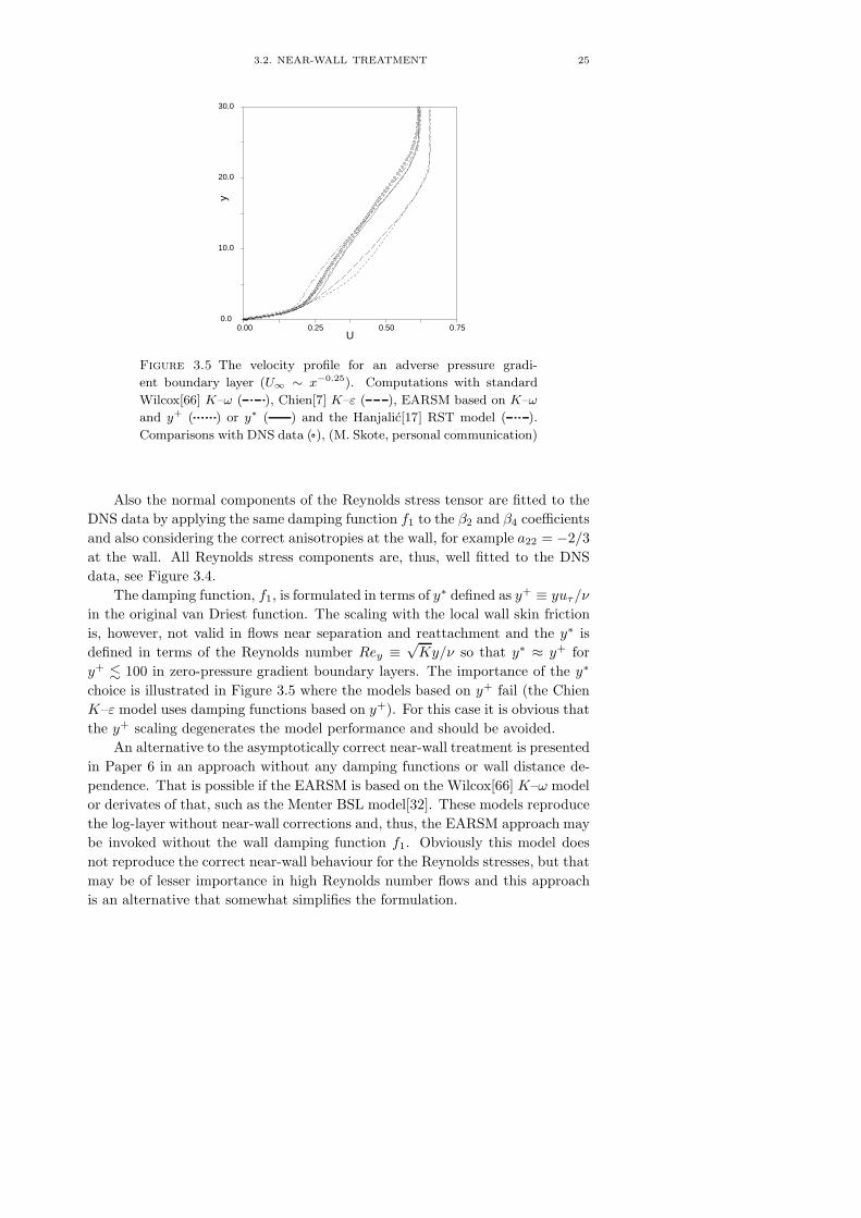
Figure 3.5 The velocity profile for an adverse pressure gradi-
ent boundary layer (U∞ ∼ x−0.25). Computations with standard
Wilcox[66] K–ω ( ), Chien[7] K–ε ( ), EARSM based on K–ω
and y+ ( ) or y∗ ( ) and the Hanjalic[17] RST model ( ).
Comparisons with DNS data ( ), (M. Skote, personal communication)
Also the normal components of the Reynolds stress tensor are fitted to theDNS data by applying the same damping function f1 to the β2 and β4 coefficientsand also considering the correct anisotropies at the wall, for example a22 = −2/3at the wall. All Reynolds stress components are, thus, well fitted to the DNSdata, see Figure 3.4.
The damping function, f1, is formulated in terms of y∗ defined as y+ ≡ yuτ/ν
in the original van Driest function. The scaling with the local wall skin frictionis, however, not valid in flows near separation and reattachment and the y∗ isdefined in terms of the Reynolds number Rey ≡ √
Ky/ν so that y∗ ≈ y+ fory+ 100 in zero-pressure gradient boundary layers. The importance of the y∗
choice is illustrated in Figure 3.5 where the models based on y+ fail (the ChienK–ε model uses damping functions based on y+). For this case it is obvious thatthe y+ scaling degenerates the model performance and should be avoided.
An alternative to the asymptotically correct near-wall treatment is presentedin Paper 6 in an approach without any damping functions or wall distance de-pendence. That is possible if the EARSM is based on the Wilcox[66] K–ω modelor derivates of that, such as the Menter BSL model[32]. These models reproducethe log-layer without near-wall corrections and, thus, the EARSM approach maybe invoked without the wall damping function f1. Obviously this model doesnot reproduce the correct near-wall behaviour for the Reynolds stresses, but thatmay be of lesser importance in high Reynolds number flows and this approachis an alternative that somewhat simplifies the formulation.

26 3. THE PROPOSED MODELLING APPROACH
3.3. Numerical behaviour and some applications
The major argument for EARSMs is to increase the validity and generalityof two-equation models without significantly increased computational cost, sothe numerical treatment is one of the cornerstones in this study in spite of therelative small attention to this in the attached papers.
3.3.1. Effective eddy viscosity. The Reynolds stresses expressed by theEARSM may be written in terms of an effective eddy viscosity νT and an extraanisotropy a
(ex)ij
uiuj =23Kδij − 2νTS∗
ij + Ka(ex)ij (38)
where the effective turbulent viscosity reads
νT = −12
(β1 + IIΩβ6)Kτ (39)
and the extra anisotropy
a(ex) = β3
(Ω2 − 1
3IIΩ I
)+ β4 (SΩ−ΩS)
+ β6
(SΩ2 +Ω2S− IIΩS− 2
3IV I
)+ β9
(ΩSΩ2 −Ω2SΩ
). (40)
The β-coefficients are given in Paper 1.This formulation is identical to that in (25) and the reason for invoking the
eddy viscosity is that many CFD solvers already have different eddy-viscositytwo-equation models implemented so the model implementation becomes easierwith a formulation in terms of an eddy viscosity. It has also been found that theextra anisotropy may be treated in a fully explicit way without degenerating theoverall performance of the solution process.
3.3.2. Positivity. It is well known that positivity of the turbulence vari-ables (K, ε) at any time during iteration to a steady-state solution is crucial. Adhoc methods, like a lower limit of the turbulent variables, often prevent the con-vergence or cause divergence of the iterative process which means that positivitymust be maintained by the numerical scheme. First, the spatial scheme mustsuppress spurious oscillations that may give negative values, which is obtainedby imposing TVD-like conditions[23]. Then the time integration method, or it-erative process, must guarantee positivity. The CFD solver EURANUS[41] usedin this study uses explicit pseudotime marching to steady state, so the positivetime integration described here will be focused on explicit methods.
In Paper 7 a novel approach is suggested for updating the turbulence vari-ables guaranteeing positivity. The approach is based on an estimate of the spec-tral radius of the complete turbulent equations and produces an underrelaxed

3.3. NUMERICAL BEHAVIOUR AND SOME APPLICATIONS 27
update of the turbulence variables q. This may be written in the following form
qn+1 = qn +∆tR(q)
1 − min(∆tR(q)/qn, 0
) . (41)
The underrelaxation depends on the local residual R(q) = ∂q/∂t and is significantonly in those regions where the residual is large compared to the variable itselfand is only active if the variable is decreasing. The method does not affect theasymptotic convergence rate and is most important initially.
Multigrid methods are important for convergence acceleration, especially forexplicit methods, and are considered in Paper 7. The update of the turbulencevariables from the prolongated correction may result in spurious oscillations thatmay cause negative values locally. Also here the method for positive updating(41) is used.
3.3.3. Compressible flow applications. A straightforward extension ofthe proposed EARSM for compressible mean flow effects is described in Paper 1.Compressible effects due to turbulent fluctuations have not been considered. Theextended EARSM was tested on a supersonic boundary layer at Mach 5 inter-acting with an impinging shock of different strengths (Schulein, Krogmann, &Stanewsky[49]). The proposed EARSM was used with both the Chien[7] K–ε andthe Wilcox[66] K–ω models as platforms and substantial differences between thebaseline two-equation models were found. The EARSM approach significantlyimproved the prediction of the size of the separation zone over the correspond-ing eddy-viscosity models, which severely underpredicted the separation length.Also the influence of different shock strengths was accurately captured, rang-ing from almost separated for the weakest shock to a large separation regionfor the strongest shock. The Chien K–ε models, both the eddy-viscosity andthe EARSM version, severely overpredicted the skin friction coefficient in thereattachment region. The K–ω models behaved much better in that respect.Detailed results are reported in Paper 2.
Figure 3.6 shows the computational results for the two-dimensional RAE2822aerofoil profile using the Wallin & Johansson EARSM compared to the Wilcox[67]K–ω model. The EARSM approach clearly improves the prediction of the posi-tion of the shock and the results are very much in line with differential Reynoldsstress computations by Hellstrom, Davidsson & Rizzi[18] for the same conditionsand geometry.
Computations are made where the damping function f1 in the EARSM isformulated in terms of y+ as well as y∗ and the figure shows no major differencesbetween these approaches except in the separated region where the y+ formu-lation gives a somewhat larger negative skin friction. The figure also shows acomputation using the proposed EARSM, together with the Wilcox[66] K–ωmodel, without any damping functions whatsoever. Even if this model is unableto reproduce the correct near-wall behaviour for the turbulence quantities, the

28 3. THE PROPOSED MODELLING APPROACH
x/c
Cp
0.0 0.2 0.4 0.6 0.8 1.0 1.0
0.5
0.0
-0.5
-1.0
-1.5
x/c
Cf
0.0 0.2 0.4 0.6 0.8 1.0 -0.006
-0.002
0.002
0.006
0.010
Figure 3.6 Wall pressure and skin friction coefficients for the
RAE2822 wing profile (M = 0.754, α = 2.57 and Re = 6.2 × 10⁶).
Predictions using Wilcox[67] K–ω ( ) and the Wallin & Johansson
EARSM based on K–ω with damping function based on y+ ( ),
y∗ ( ) or without any damping functions ( ), compared to ex-
perimental data ( ) by Cook et al.[8]. The geometry is the measured
one including a camber correction.
mean velocity profiles are well reproduced and there are no major differencesbetween the EARSM with or without damping functions.
The convergence history is shown in figure 3.7 where we can see that thereare no major differences in convergence rate between the different approaches.Actually, the proposed EARSM converges to a somewhat lower residual than thecorresponding eddy-viscosity model for this case. The numerical parameters arethe same for these two cases and the computational time for the 5000 iterationsteps is 6% higher for the EARSM computation. This case was found not tobe completely numerically stationary which results in the residual ‘hanging’ asfor the K–ω model. The fluctuations are, however, very small and could not beseen in the solution. In other cases without separation the convergence curvesare even closer to each other, and the convergence rates are in general fasterthan for the case shown in figure 3.7.

3.4. TIME-DEPENDENT TURBULENCE 29
iter
rho_
rms
0. 2000. 4000. 6000. -6.0
-4.0
-2.0
0.0
Figure 3.7 Convergence history for the RAE2822 wing profile.
Wilcox[67] K–ω ( ) compared with the Wallin & Johansson
EARSM based on K–ω ( ). The computational time is increased
by 6% by using EARSM. Three levels of full multigrid is used.
A further example with a three-dimensional transonic supercritical wing wascomputed using the standard Wilcox[66] K–ω model and the EARSM based onthat, see Paper 6. Again, the predicted shock position was found to be improvedcompared to the eddy-viscosity model. This case illustrates the benefit of theproposed model which is also viable in expensive three-dimensional cases, herewith almost one million grid points. Most importantly, there is no substan-tial increase in the computational cost compared to the, in many cases, robuststandard K–ω model.
3.4. Time-dependent turbulence
The mean flow is considered as unsteady when the time scale of the unsteadi-ness is much larger than the characteristic integral time scale of the turbulence.In that case the turbulence energy spectrum is well separated from the unsteadi-ness. Thus, the turbulence may be modelled while the mean flow unsteadinessis left to be resolved in the unsteady RANS solution. This is known as thequasi-steady approach where a standard RANS turbulence model, with the timederivatives included, may be used. No additional modification of the turbulencemodel is in principal needed due to the unsteadiness.
If there is no clear separation between the turbulence scales and the unsteadi-ness, then standard RANS turbulence models should not be used. Therefore thisclass of problems needs to be tackled using large eddy simulations (LES) wheresubgrid-scale models are used to represent the unresolved stresses. The Reynoldsaveraged and the filtered Navier-Stokes equations are in principal similar, butthe unknown correlation uiuj is modelled in completely different ways in RANS

30 3. THE PROPOSED MODELLING APPROACH
Table 3.2 Computed reduced frequency for unsteady transonic air-
foil flow compared to experiment by McDevitt[34].
model EARSM K–ω B–L Exp.reduced frequency 0.493 0.441 0.461 ∼ 0.49
and LES. A RANS model could not be used as a subgrid-scale model, mainlybecause a RANS model is unable to capture the decreased subgrid-scale energywith decreased filter width. Actually, it gives the opposite trend of increasededdy viscosity.
Unsteady turbulent flows are often by nature, or forced to be, periodic andthe mean is thus conveniently defined as a phase average. The flow variablesare decomposed into three parts, φ = φ + φ” + φ, where φ is the time-averagedvalue, φ” is the periodic component and φ the turbulent fluctuations. The phase-averaged variable is then defined as 〈φ〉 ≡ φ + φ”.
In the quasi-steady approach, RANS turbulence models will be used withoutany explicit modifications due to the unsteadiness. However, the unsteadinessof the mean flow poses some additional requirements on the turbulence model,or will emphasize existing requirements on models for steady flows even more.The following general requirements can thus be identified: (i) No y+ or log-lawdependency, (ii) correct near-wall asymptotic behavior, (iii) good prediction ofnonequilibrium turbulence and (iv) good prediction of boundary layer separation.The Wallin & Johansson EARSM is thus a good candidate also for modellingunsteady turbulent flows.
The periodic self-excited turbulent flow around an 18-percent thick circular-arc airfoil at transonic speeds has been computed in Paper 4 using three differentturbulence models: the Baldwin & Lomax (B–L) algebraic model[3], the WilcoxK−ω model[67], and the Wallin & Johansson EARSM. The EARSM predicts theunsteadiness due to shock and boundary layer separation better than the eddy-viscosity models. The EARSM predicts the frequency of self-exited unsteadytransonic flow to high accuracy, see Table 3.2, and the motion of the shockagrees well with the experimental data.
3.5. Passive scalar modelling
In Paper 5 an explicit algebraic relation for the scalar flux is proposed. Thisis intended to be used in an explicit algebraic approximation approach for thetransport equations for the Reynolds stress tensor and scalar flux vector. Therelation for the scalar flux vector is derived by neglecting the advection anddiffusion of the normalized scalar flux uiθ/
√KKθ. This gives in general an
implicit, nonlinear set of algebraic equations. The nonlinearity in the algebraicequations for the normalized scalar fluxes may be eliminated directly by using anonlinear term in the model of the pressure scalar-gradient correlation and the

3.5. PASSIVE SCALAR MODELLING 31
Table 3.3 Predicted scalar fluxes in homogeneous shear flow using
the WWJ model proposed in Paper 5 compared to the DNS data of
Rogers et al.[44]. Case 1, 2 and 3 corresponds to a scalar gradient in
the streamwise, cross-stream and spanwise directions respectively.
Case 1 Case 2 Case 3uθ vθ uθ vθ wθ
DNS data −2.41 0.45 0.94 −0.36 −0.67WWJ model −2.05 0.42 1.13 −0.46 −0.70
0 0.2 0.4 0.6 0.8 1−2
0
2
4
6
η
Figure 3.8 Predicted scalar fluxes in the channel flow using the
WWJ model ( ) compared to DNS data for −uθ (∗) and vθ () ofWikstrom et al.[64]. The predicted fluxes were evaluated from (42)
by use of the DNS data.
destruction and thus results in an algebraically simple model for both two- andthree-dimensional mean flows. The resulting model may be written as
uiθ = −A−1ij ujuk
K
ε
∂Θ∂xk
(42)
where the tensor A−1ij is an explicit function of the normalized mean velocity
gradients τ∂Ui/∂xj , the production to dissipation ratio P/ε and the ratio of thescalar to dynamical timescales r.
The proposed model is, however, not complete since transport equations forthe scalar variance θ2 ≡ 2Kθ and its dissipation rate εθ are needed for obtainingthe timescale ratio r. The modelling of these equations is not considered inPaper 5. These issues are investigated to some extent in Johansson & Wikstrom[21].
The performance of the present model is investigated in three different flowsituations in Paper 5. These are homogeneous shear flow with an imposed mean

32 3. THE PROPOSED MODELLING APPROACH
0 0.5 1 1.5 2 2.5−0.1
−0.08
−0.06
−0.04
−0.02
0
0.02
0.04
0.06
η
Figure 3.9 Predicted scalar fluxes in the cylinder wake using the
WWJ model ( ) compared to experimental data for −uθ (∗) andvθ () of Wikstrom et al.[65]. The predicted fluxes were evaluated
from (42) by use of the experimental data.
scalar gradient (Table 3.3), turbulent channel flow (Figure 3.8), and the flow fielddownstream a heated cylinder (Figure 3.9). DNS data are used to analyse thepassive scalar flux in the homogeneous shear and channel flow cases, and exper-imental data are used in the case of the heated cylinder wake. Good predictionsin all three cases are demonstrated. It is interesting to note that, both for thechannel flow and the heated cylinder wake, uθ and vθ are of the same orderof magnitude. This is well captured by the EASFM, whereas eddy-diffusivitymodels would predict a zero uθ.
CHAPTER 4
Conclusions and outlook
The ultimate goal in turbulence modelling is to obtain a universally validmodel. Since that is, by far, out of reach, a more realistic goal must be setand could be what Pope[37] referes to as an optimal turbulence model. This hedefines as the best particular model within each class of models. For a givensuch class of models, the validity and generality should be increased to the limitof the applicability of that class. In this effort one really needs to be aware ofthe physical limitations for different types of models.
This work fits into the efforts to increase the validity and generality of two-equation models during the last decade by abandoning the eddy-viscosity hy-pothesis. Bradshaw[6] writes ”Using eddy viscosity is like keeping one foot onthe bottom when learning to swim – a restriction, but helpful if one does notventure into deep water”, an argument that can be used both for keeping andleaving the eddy-viscosity hypothesis. The improvements result in more generalconstitutive relations between the second moments (uiuj and uiθ) and the meanflow.
The proposed models are the results of careful and well-motivated approx-imations of the corresponding second-order transport model equations. Themajor advantage of this approach compared to more empirical nonlinear exten-sions to eddy-viscosity models is that the model coefficients and behaviour of thefull second-order model is inherited in the algebraic form. This means that it ispossible to estimate the validity of the model prediction based on the expectedbehaviour of the full second-order model and the validity of the approximations.Empirical extensions of eddy-viscosity models have many degrees of freedom andmay be adjusted to a large number of different test cases. These kind of modelscould, however, not with confidence be extended outside of the range of the setof validation and calibration cases used for finding appropriate functional formsand calibration of the different terms.
The EARSM proposed in Paper 1 is derived from the recalibrated LRRmodel. The method, at least for two-dimensional mean flows, are general andthe EARSM could in principal be derived also from the linearized SSG model.There is actually a strong argument for deriving the EARSM from the SSGmodel and that is that the SSG model has previously been found to performbetter than LRR in a number of cases, especially in nonequilibrium and rotatingflows. The LRR used in this study was, however, found to give results comparable
33

34 4. CONCLUSIONS AND OUTLOOK
to the SSG when used in the algebraic forms and after recalibration of the LRRmodel coefficients. An explanation of why the algebraic forms perform moresimilarly than the corresponding full differential forms has been proposed. Theslight degeneration in model performance using EARSM derived from LRR iswell balanced by the fact that the full three-dimensional form of the proposedEARSM is simple enough to be useful only for the EARSM derived from LRR.The full three-dimensional form is necessary for capturing, for instance, thesecondary swirl in axially rotating pipes.
In the case of strong streamline curvature, the weak-equilibrium assumptionmust be derived in a streamline based coordinate system. In some specific cases,such as symmetric vortices and rotating homogeneous shear flows, the streamlinebased coordinate system may explicitly be defined and the advection term maybe exactly included into the EARSM form. For these specific cases the propertreatment of the advection term has been found to be of crucial importance.When approximations of the advection term is included into the EARSM formu-lation, the proposed EARSM fails because of the basic LRR model. However, byan ad hoc modification of the coefficient preceding the complete right-hand sideof the anisotropy transport equation (19), it is possible to get a model behavioursimilar to EARSM derived from SSG in these kind of flows and also keeping thesimplified three-dimensional form.
One should here start to consider if it is worth the effort to include approx-imations of the transport terms from the full RST model within the EARSMform instead of leaving this class of models for full RST models where such ef-fects enters naturally. The only, and so far completely relevant, argument forEARSM is the troublesome numerical treatment and computational cost of fullRST models. One should, thus, put more efforts on improvements of the numer-ical methods for full RST models and entice specialists in numerical methods toleave the island of constant coefficients for the world of these strongly nonlinearproblems. Hopefully, one would expect that improvements in numerical methodsand computer performance would decrease the importance of the argument forEARSM in the near future and, thus, the importance of RST models in engineer-ing CFD methods could be expected to increase. Also in such a situation it isworthwhile to continue the struggle for the search of the ‘optimal’ model withinboth the class of two-equation models and that of full differential Reynolds stressmodels.

Acknowledgments
I wish to thank my supervisor Professor Arne Johansson for introducing meinto the field of turbulence modelling. During our numerous discussions, whichhe always had time for, Arne guided me with his great knowledge in this field.The atmosphere at the department has been inspiring and friendly. I wouldespecially like to thank Doctor Petra Wikstrom for a fruiful collaboration onpassive scalars and Martin Skote for providing me with DNS data.
I also wish to thank Doctor Ingemar Lindblad, head of my department atFFA, for believing in my ideas and supporting me even when I seemed to havedisappeared into the boundary layer. The professionalism and wide range ofexperience of my colleagues at FFA were the prerequisite and basis of my work.I particularly want to thank Doctor Peter Eliasson for helping me with numericaltreatment and implementation issues.
I would like to thank Doctor Torbjorn Sjogren for our discussions concerningrepresentation theory and automatic code generation. Professor Sharath Giri-maji is kindly acknowledged for fruitful discussions and for making the visit ofme and my family at ICASE very pleasant.
Finally, I want to thank Ingela for always supporting me. Tack Tommy ochCecilia for att ni ar sa mysiga.
Financial support from FFA, ESA, EU, NUTEK and FMV is gratefullyacknowledged.
35

Bibliography
[1] Abe, K., Kondoh, T. & Nagano, Y. 1996 A two-equation heat transfer model reflecting
second-moment closures for wall and free turbulent flows. Int. J. Heat and Fluid Flow 17,
228-237.
[2] Adumitroaie, V., Taulbee, D.B. & Givi, P. 1997 Explicit Algebraic Scalar-Flux Models
for Turbulent Reacting Flows. A. i. ch. e. J. 8, 1935-2147.
[3] Baldwin, B. & Lomax, H. 1978 Thin Layer Approximation and Algebraic Model for
Separated Turbulent Flow. AIAA Paper 78-257.
[4] Bardina, J., Ferziger, J.H. & Reynolds, W.C. 1983 Improved turbulence models based
on large-eddy simulation of homogeneous, incompressible turbulent flows. Stanford Uni-
versity Tech. Rep. TF-19.
[5] Boussinesq, J. 1877 Essai sur la theorie des eaux courantes. Mem. pres. Acad. Sci., 3rd
edn, Paris XXIII, 46.
[6] Bradshaw, P. 1997 The best turbulence models for engineers. In Modeling complex tur-
bulent flows, Eds. M.D. Salas, J.N. Hefner, L. Sakell, Kluwer (1999).
[7] Chien, K.Y. 1982 Predictions of Channel and Boundary-Layer Flows with a Low-
Reynolds-Number Turbulence Model. AIAA J. 20, 33–38.
[8] Cook, P.H., MacDonald, M.A. & Firmin, M.C.P. 1979 Aerofoil 2822 - Pressure distri-
butions, boundary layer and wake measurements. AGARD AR 138.
[9] Craft, T.J., Launder, B.E. & Suga, K. 1993 Extending the applicability of eddy viscos-
ity models through the use of deformation invariants and non-linear elements. In Proc. 5th
Int. Symp. on Refined Flow Modelling and Turbulence Measurements, 125–132, Presses
Ponts et Chaussees, Paris.
[10] Daly, B.J. & Harlow, F.H. 1970 Transport equations in turbulence. Phys. Fluids 13,
2634–2649.
[11] Friedrich, R. 1998 Modelling of turbulence in compressible flows. Chapter 5 of Transi-
tion, Turbulence and Combustion Modelling, Eds. A. Hanifi, P.H. Alfredsson, A.V.
Johansson and D.S. Henningson. Kluwer.
[12] Gatski, T.B & Speziale C.G. 1993 On explicit algebraic stress models for complex
turbulent flows. J. Fluid Mech. 254, 59–78.
[13] Girimaji, S.S. 1996 Fully-explicit and self-consistent algebraic Reynolds stress model
Theor. and Comp. Fluid Dyn. 8 387–402 (also ICASE Report No. 95-82).
[14] Girimaji, S.S. 1997 A Galilean invariant explicit algebraic Reynolds stress model for
turbulent curved flows Phys. Fluids. 9 1067–1077 (also ICASE Report No. 96-38).
[15] Girimaji, S.S. 1997 Development of algebraic Reynolds stress model for non-equilibrium
turbulence. In Modeling complex turbulent flows, Eds. M.D. Salas, J.N. Hefner, L. Sakell,
Kluwer (1999).
[16] Girimaji, S.S. & Balachandar, S. 1998 Analysis and modeling of boyancy-generated
turbulence using numerical data. Int. J. Heat Mass Transfer 41, 915-929.
36

BIBLIOGRAPHY 37
[17] Hanjalic, K., Jakirlic, S. & Hadzic, I. 1995 Computation of oscillating turbulent flows
at transitional Re-numners Turbulent Shear Flows 9 pp 323–342. Eds F. Durst, N. Kasagi
& B.E. Launder. Springer-Verlag, Berlin.
[18] Hellstrom, T., Davidson, L. & Rizzi, A. 1994 Reynolds stress transport modelling
of transonic flow around the RAE2822 airfoil. AIAA 94-0309 32nd Aerospace Sciences
Meeting, Reno, Jan 1994
[19] Johansson, A.V. & Burden, A.D. 1998 An introduction to turbulence modelling. Chap-
ter 4 of Transition, Turbulence and Combustion Modelling, Eds. A. Hanifi, P.H.
Alfredsson, A.V. Johansson and D.S. Henningson. Kluwer.
[20] Johansson, A.V. & Wallin, S. 1996 A new explicit algebraic Reynolds stress model.
Proc. Sixth European Turbulence Conference, Lausanne, July 1996, Ed. P. Monkewitz,
31–34.
[21] Johansson, A.V. & Wikstrom, P.M. 2000 DNS and modelling of passive scalar transport
in turbulent channel flow with a focus on scalar dissipation rate modelling. To appear in
ERCOFTAC J.
[22] Jones, W.P. & Launder, B.E. 1972 The prediction of laminarization with a two-equation
model of turbulence. Int. J. Heat Mass Trans. 15, 310–314.
[23] Jongen, T. & Marx, Y.P. 1997 Design of an unconditionally stable positive scheme for
the K–ε and two-layer turbulence models. Computers & Fluids 26, 469–487.
[24] Jongen, T., Machiels, L. & Gatski, T.B. 1998 Predicting noninertial effects with linear
and nonlinear eddy-viscosity, and algebraic stress models. Flow Turbul. Combust. 60 (2),
215–234.
[25] Jongen, T. & Gatski, T.B. 1998 A new approach to characterizing the equilibrium
states of the Reynolds stress anisotropy in homogeneous turbulence. Theoret. Comput.
Fluid Dynamics 11, 31–47.
[26] Jongen, T., Mompean, G. & Gatski, T.B. 1998 Predicting S-duct flow using a composite
algebraic stress model. AIAA J. 36, 327–335.
[27] Kolmogorov, A.N. 1942 Equations of turbulent motions of an incompressible fluid. Izves-
tia Academy of Sciences, USSR; Physics, 6, 56–58.
[28] Launder, B.E. 1978 Heat and mass transport. In Turbulence, P. Bradshaw (ed.), Springer,
Berlin, 231-287.
[29] Launder, B.E., Reece, G.J. & Rodi, W. 1975 Progress in the development of a Reynolds-
stress turbulence closure. J. Fluid Mech. 41, 537–566.
[30] Lumley, J.L. 1978 Computational modeling of turbulent flows. Adv. Appl. Mech. 18,
123–176.
[31] Launder, B.E. 1996 Advanced turbulence models for industrial applications Chapter 5
of Turbulence and Transition Modelling, Eds. M. Hallback, D.S. Henningson, A.V.
Johansson and P.H. Alfredsson. Kluwer.
[32] Menter, F.R. 1994 Two-equation eddy-viscosity turbulence models for engineering ap-
plications. AIAA J. 32, 1598–1604.
[33] Moser, R.D, Kim J. & Mansour N.N. 1998 DNS of Turbulent Channel Flow up to
Reτ = 590. Phys. Fluids 11, 943–945.
[34] McDevitt, J. 1979 Supercritical Flow about a Thick Circular-Arc Airfoil. NASA TM-
78549.
[35] Naot, D., Shavit, A. & Wolfstein, M. 1973 Two-point correlation model and the
redistribution of Reynolds stresses. Phys. Fluids 16, 738–743.
[36] Pope, S.B. 1975 A more general effective-viscosity hypothesis J. Fluid Mech. 72, 331–340.
[37] Pope, S.B. 1997 A perspective on turbulence modeling. In Modeling complex turbulent
flows, Eds. M.D. Salas, J.N. Hefner, L. Sakell, Kluwer (1999).
[38] Prandtl, L. 1925 Uber die ausgebildete Turbulenz. ZAMM 5, 136–139.

38 BIBLIOGRAPHY
[39] Prandtl, L. 1945 Uber ein neues Formelsystem fur die ausgebildete Turbulenz. Nachr.
Akad. Wiss. Gottingen. Math.-Phys. Kl. 1945, 6–19.
[40] Reynolds, O. 1883 An experimental investigation of the circumstances which determine
whether the motion of water shall be direct or sinuous, and of the law of resistance in
parallel channels. Philos. Trans. R. Soc. London 174, 935–982.
[41] Rizzi, A., Eliasson, P., Lindblad, I., Hirsch C., Lacor, C., Haeuser, J. 1993 The
engineering of multiblock/multigrid software for Navier-Stokes flows on structured meshes
Computers Fluids 22, 341–367.
[42] Rodi, W. 1972 The prediction of free turbulent boundary layers by use of a two equation
model of turbulence. Ph.D. thesis, University of London.
[43] Rodi, W. 1976 A new algebraic relation for calculating the Reynolds stresses. Z. angew.
Math. Mech. 56, T219–221.
[44] Rogers, M.M., Moin, P. & Reynolds, W.C. 1986 The structure and modeling of the
hydrodynamic and passive scalar fields in homogeneous turbulent shear flow. Dept. Mech.
Engng. Rep. TF-25, Stanford University, Stanford, California.
[45] Rogers, M.M., Mansour, P. & Reynolds, W.C. 1989 An algebraic model for the tur-
bulent flux of a passive scalar. J. Fluid Mech. 203, 77-101.
[46] Rotta, J.C. 1951 Statistische Theorie nichthomogener Turbulenz. Z. Phys. 129, 547–572.
[47] Rumsey, C.L., Gatski, T.L. & Morrison, J.H. 1999 Turbulence model predictions of
extra-strain rate effects in strongly-curved flows. AIAA Paper 99-157
[48] Rung, T., Lubcke, H., Franke, M., Xue, L., Thiede, F. & Fu, S. 1999 Assessment
of explicit algebraic stress models in transonic flows. In Proc. Eng. turb. modelling and
experiments 4, Ajaccio, France, May 1999, Elsevier.
[49] Schulein, E., Krogmann, P. & Stanewsky, E. 1996 Documentation of Two-Dimensional
Impinging Shock/ Turbulent Boundary Layer Interaction Flow. DLR Report: DLR IB 223
- 96 A 49.
[50] Shabany, Y. & Durbin, P.A. 1997 Explicit algebraic scalar flux approximation. AIAA
J. 35, 985-989.
[51] Shabbir, A. & Shih, T.H. 1992 Critical Assessment of Reynolds Stress Turbulence Models
Using Homogeneous Flows NASA TM 105954, ICOMP-92-24, CMOTT-92-12.
[52] Shih, T.H. & Lumley, J.L. 1993 Remarks on Turbulent Constitutive Relations. Mathl.
Comput. Modelling 18(2), 9-16.
[53] Shih, T.H., Zhu, J. & Lumley, J.L. 1992 A Realizable Reynolds Stress Algebraic Equa-
tion Model NASA TM 105993, ICOMP-92-27, CMOTT-92-14.
[54] Shih, T.-H. 1996 Constitutive relations and realizability of single-point turbulence clo-
sures Chapter 4 of Turbulence and Transition Modelling, Eds. M. Hallback, D.S.
Henningson, A.V. Johansson and P.H. Alfredsson. Kluwer.
[55] Sjogren, T. 1997 Development and Validation of Turbulence Models Through Experi-
ment and Computation Doctoral thesis, Dept. of Mechanics, KTH, Stockholm, Sweden.
[56] Sjogren, T. & Johansson, A.V. 1999 Development and calibration of algebraic non-
linear models for terms in the Reynolds stress transport equations To appear in Phys.
Fluids
[57] Spalart P.R. & Speziale, C.G. 1999 A note on constraints in turbulence modelling.
J. Fluid Mech. 391, 373–376.
[58] Spalart P. & Allmaras, S.R. 1992 A one-equation model for aerodynamic flows. AIAA
paper 92-439.
[59] Spencer, A.J.M. & Rivlin, R.S. 1959 The theory of matrix polynomials and its appli-
cation to the mechanics of isotropic continua Arch. Rat. Mech. Anal. 2, 309–336.
[60] Speziale, C.G., Sarkar, S. & Gatski, T.B. 1991 Modelling the pressure-strain cor-
relation of turbulence: an invariant dynamical systems approach. J. Fluid Mech. 227,
245–272.

BIBLIOGRAPHY 39
[61] Speziale, C.G. & Xu, X.-H. 1996 Towards the development of second-order closure mod-
els for nonequilibrium turbulent flows Int. J. Heat and Fluid Flow 17, 238–244.
[62] Taulbee, D.B. 1992 An improved algebraic Reynolds stress model and corresponding
nonlinear stress model. Phys. Fluids A 4, 2555–2561.
[63] Tennekes, H. & Lumley, J.L. 1972 A first course in turbulence. The MIT Press, Cam-
bridge, MA, and London, England.
[64] Wikstrom, P.M. & Johansson, A.V. 1998 DNS and scalar-flux transport modelling in a
turbulent channel flow. In proc. Turbulent Heat Transfer II, May 31-June 5, Manchester.
[65] Wikstrom, P.M., Hallback, M., & Johansson, A.V. 1998 Measurements and heat-flux
transport modelling in a heated cylinder wake. Intl. J. Heat Fluid Flow 19, 556–562.
August 1998.
[66] Wilcox, D.C. 1988 Reassessment of the scale-determining equation for advanced turbu-
lence models. AIAA J. 26, 1299–1310.
[67] Wilcox, D.C. 1994 Simulation of Transition with a Two-Equation Turbulence Model.
AIAA J. 32, 247–255.
[68] Xu, X.-H. & Speziale, C.G. 1996 Explicit algebraic stress model of turbulence with
anisotropic dissipation. AIAA J. 34, 2186–2189.


Paper 1
1


AN EXPLICIT ALGEBRAIC REYNOLDS STRESS MODELFOR INCOMPRESSIBLE AND COMPRESSIBLE TURBULENT
FLOWS
Stefan Wallin
The Aeronautical Research Institute of Sweden (FFA)
Box 11021, SE-16111 Bromma, Sweden
Arne V. Johansson
Department of Mechanics, KTH, SE-100 44 Stockholm, Sweden
Abstract. Some new developments of explicit algebraic Reynolds stress
turbulence models (EARSM) are presented. The new developments include
a new near-wall treatment ensuring realizability for the individual stress
components, a formulation for compressible flows, and a suggestion for
a possible approximation of diffusion terms in the anisotropy transport
equation. Recent developments in this area are assessed and collected into
a model for both incompressible and compressible three-dimensional wall-
bounded turbulent flows. This model represents a solution of the implicit
ARSM equations, where the production to dissipation ratio is obtained as
a solution to a nonlinear algebraic relation. Three-dimensionality is fully
accounted for in the mean flow description of the stress anisotropy. The
resulting EARSM has been found to be well suited to integration to the wall
and all individual Reynolds stresses can be well predicted by introducing
wall damping functions derived from the van Driest damping function. The
platform for the model consists of the transport equations for the kinetic
energy and an auxiliary quantity. The proposed model can be used with
any such platform, and examples are shown for two different choices of the
auxiliary quantity.
1. Introduction
Standard two-equation models are still dominant in the context of industrialflow computations. In flows with strong effects of streamline curvature, adversepressure gradients, flow separation or system rotation, such models fail to giveaccurate predictions. Turbulence models based on the transport equations forthe individual Reynolds stresses have the natural potential for dealing with, forexample, the associated complex dynamics of inter-component transfer. TheBoussinesq hypothesis may in this context be said to be replaced by transportequations for the individual Reynolds stress anisotropies. As yet, there are non-trivial numerical aspects of flow computations with such models in complexflow situations. This represents an active area of research. In parallel with suchefforts there has been a considerable renewed interest in various forms of algebraicapproximations of the anisotropy transport equations. In the present work somenew developments are presented for explicit formulations of algebraic Reynolds
43

44 AN EXPLICIT ALGEBRAIC REYNOLDS STRESS MODEL
stress models. The motivation for this work is the general need for improvementsin the prediction of complicated turbulent flows using the platform of existingCFD prediction tools based on the two-equation modelling level.
1.1. Algebraic Reynolds stress models. The classical algebraic Reynoldsstress model (ARSM), Rodi[26, 27], was developed from the modelled Reynoldsstress transport (RST) equation by assuming that the advection minus the dif-fusion of the individual Reynolds stresses can be expressed as the product of thecorresponding quantity for the kinetic energy, K, and the individual Reynoldsstresses normalized by K. This results in an implicit relation between the stresscomponents and the mean velocity gradient field that replaces the Boussinesqhypothesis. Since the algebraic Reynolds stress model is determined from themodelled Reynolds stress transport equation no additional model constants areneeded and the basic behaviour and experiences of the particular RST modelwill be inherited. The linearity of the Boussinesq hypothesis excludes any de-pendence on the rotational (antisymmetric) part of the mean velocity gradienttensor. An ARSM approach here represents a systematic method of constructinga nonlinear stress relationship that includes effects of the rotational part of themean velocity gradient tensor. Despite this definite improvement one should,however, keep in mind that the ARSM can never represent the transport effectsas well as a full RST model, which always should be expected to give a morecorrect description of the turbulence. Also, the RST models have limitations inpredicting turbulence for general and complicated flows, especially in describingthe effects of rotation.
The traditional ARSM idea is equivalent to neglecting advection and diffusionterms in the exact transport equation for the Reynolds stress anisotropy, aij ,defined as aij ≡ uiuj/K − 2δij/3. The advection term is indeed exactly zero forall stationary parallel mean flows, such as fully developed channel and pipe flows.For inhomogeneous flows the assumption of negligible effects of diffusion in theaij equation can cause problems, particularly in regions where the productionterm is small or where the inhomogeneity is strong. However, the Rodi ARSMassumption incorporates in a natural way not only effects of rotation but alsoeffects of streamline curvature and three-dimensionality of the flow and has beenfound to be a reasonable approximation of the full differential RST equationsin a number of flow situations, in many respects superior to the eddy-viscosityhypothesis.
To illustrate the natural way in which system rotation, and rotational effectsin general, enter in this type of formalism we may take as the starting pointthe transport equation for the Reynolds stress anisotropy tensor in a rotatingCartesian coordinate system (the formulation of algebraic Reynolds stress modelsfor rotating and curvilinear coordinate systems has recently been studied in some

STEFAN WALLIN AND ARNE V. JOHANSSON 45
detail by Sjogren[35])
KD aij
Dt−(∂Tijl
∂xl− uiuj
K
∂T(K)l
∂xl
)= −uiuj
K(P − ε) + Pij − εij + Πij + εC
(a)ij
(1)
where −Tijl and −T (K)l are the fluxes (turbulent and molecular) of the Reynolds
stress and turbulent kinetic energy, respectively. The dissipation rate tensor, εij ,and the pressure strain, Πij , need to be modelled whereas the production terms,Pij and P = Pii/2, and the Coriolis term, C(a)
ij , do not need any modelling sincethey are explicit in the Reynolds stress tensor. In a non-rotating coordinatesystem the Reynolds stress production term is normally written as
Pij = −uiukUj,k − ujukUi,k, (2)
where Ui,j denotes the mean velocity gradient tensor. In a rotating systemit is convenient to split the mean velocity gradient tensor into a mean strainand a mean rotation tensor. We will here let Sij and Ωij denote these tensorsnormalized with the turbulent timescale, τ ≡ K/ε,
Sij =τ
2(Ui,j + Uj,i) , Ωij =
τ
2(Ui,j − Uj,i) . (3)
A consistent formulation of (1), valid also in the rotating system, can then beobtained by replacing the mean rotation tensor by the absolute rotation tensor
Ω∗ij = Ωij + Ωs
ij , (4)
where
Ωsij = τεjikω
sk (5)
and ωsk is the constant angular rotation rate vector of the system. This procedure
illustrates the origin of the two parts of what normally is referred to as theCoriolis term in the aij equation. In this way the first part is included in theproduction term, that now (normalized with ε) can be expressed as
Pij
ε= −4
3Sij − (aikSkj + Sikakj) + aikΩ∗
kj − Ω∗ikakj . (6)
The second part of the Coriolis term arises from the transformation of theadvection term. This part (normalized by ε) is denoted by C
(a)ij in (1), and can
be expressed as
C(a)ij = aikΩs
kj − Ωsikakj . (7)
The ARSM assumption results in the following implicit algebraic equation foraij :
uiuj
K(P − ε) = Pij − εij + Πij + εC
(a)ij , (8)

46 AN EXPLICIT ALGEBRAIC REYNOLDS STRESS MODEL
the structure of which, of course, depends on the choice of the models for εijand Πij . For the present modelling purpose we choose an isotropic assumptionfor the dissipation rate tensor,
εij =23εδij , (9)
and the Rotta model[28] for the slow pressure strain
Π(s)ij = −c1εaij . (10)
For the rapid pressure–strain rate we choose the general linear model of Launder,Reece & Rodi[17], which for a non-rotating system normally is written as
Π(r)ij = −c2 + 8
11
(Pij − 2
3Pδij
)− 30c2 − 2
55K (Ui,j + Uj,i)
− 8c2 − 211
(Dij − 2
3Pδij
)(11)
where Dij = −uiukUk,j − ujukUk,i.A simple way of obtaining a consistent, frame-independent formulation of the
rapid pressure–strain rate model is to apply the same methodology as for theproduction term. This gives
Π(r)ij
ε=
45Sij +
9c2 + 611
(aikSkj + Sikakj − 2
3akmSmkδij
)+
7c2 − 1011
(aikΩ∗
kj − Ω∗ikakj
). (12)
From (8) we then obtain the implicit algebraic equation for the Reynoldsstress anisotropy tensor in the form(
c1 − 1 +Pε
)a = − 8
15S+
7c2 + 111
(aΩR −ΩRa
)− 5 − 9c2
11
(aS+ Sa− 2
3traSI
)(13)
In equation (13) a, S and Ω denote second-rank tensors, and I is the identitymatrix. The inner product of two matrices is defined as (SS)ij ≡
(S2)ij≡ SikSkj
and tr denotes the trace. This notation will be kept through this paper. Oneshould note that (13) represents a nonlinear relation since P/ε ≡ −traS.
It is interesting to note that the ‘effective’ mean rotation rate tensor, ΩRij ,
depends on the choice of model:
ΩRij = Ω∗
ij +11
7c2 + 1Ωs
ij = Ωij +7c2 + 127c2 + 1
Ωsij . (14)
The ARSM approximation of the aij transport equation with this approach isthen equivalent to neglecting the advective term (and diffusion) in the chosenrotating coordinate system. Hence, the adequacy of the ARSM approach iscoupled to the choice of a coordinate system where the omission of advection

STEFAN WALLIN AND ARNE V. JOHANSSON 47
terms in the aij equation can be justified. The choice of coordinate system isnot at all trivial in strongly curved flows and the coordinate direction is not ingeneral aligned with the flow direction. There are, however, methods to constructARSMs that generally neglect only the advection term in the streamline direction(see e.g. Girimaji[10] and Sjogren[35]).
As is seen from equation (13) the treatment of system rotation is quite straight-forward. The superscript R on the mean rotation rate tensor will be dropped inthe following.
The turbulent kinetic energy, K ≡ uiui/2, and its dissipation, ε, are deter-mined from transport equations
DK
Dt+∂T
(K)l
∂xl= P − ε, (15)
D ε
Dt+∂T
(ε)l
∂xl= (Cε1P − Cε2fεε)
ε
K. (16)
There is no direct influence of system rotation on these equations. A substantialimprovement over the eddy-viscosity model equations is that the productionterm, P, does not need to be modelled. The transport terms, T (K)
l and T(ε)l , are
usually modelled using gradient diffusion with the diffusivity coefficient expressedwith the aid of the eddy viscosity, but here an improvement can also be achievedby using the knowledge of the complete Reynolds stress tensor. The gradient-diffusion model proposed by Daly & Harlow[3] applied to the turbulent kineticenergy and its dissipation gives
T(K)l = −c′s
K
εulum
∂K
∂xm, T
(ε)l = −cεK
εulum
∂ε
∂xm. (17)
Launder, Reece & Rodi[17] recommend c′s = 0.25 and cε = 0.15.
1.2. Explicit algebraic Reynolds stress models. The implicit relation fora in the ARSM equations has been found to be numerically and computation-ally cumbersome since there is no diffusion or damping present in the equationsystem. In many applications the computational effort has been found to beexcessively large and the benefits of using ARSM instead of the full Reynoldsstress model are then lost. An explicit algebraic Reynolds stress model, EARSM,where the Reynolds stresses are explicitly related to the mean flow field is muchmore numerically robust and has been found to have almost a negligible effecton the computational effort as compared to a K–ε model.
The most general form for a in terms of S and Ω consists of ten tensoriallyindependent groups to which all higher-order tensor combinations can be reduced

48 AN EXPLICIT ALGEBRAIC REYNOLDS STRESS MODEL
with the aid of the Caley–Hamilton theorem:
a = β1S+ β2
(S2 − 1
3IIS I
)+ β3
(Ω2 − 1
3IIΩ I
)+ β4 (SΩ−ΩS)
+ β5(S2Ω−ΩS2
)+ β6
(SΩ2 +Ω2S− 2
3IV I
)+ β7
(S2Ω2 +Ω2S2 − 2
3V I)
+ β8(SΩS2 − S2ΩS
)+ β9
(ΩSΩ2 −Ω2SΩ
)+ β10
(ΩS2Ω2 −Ω2S2Ω
). (18)
The β-coefficients may be functions of the five independent invariants of S andΩ, which can be written as
IIS = trS2, IIΩ = trΩ2, IIIS = trS3, IV = trSΩ2, V = trS2Ω2.(19)
Other scalar parameters may also be involved.The independence of the ten groups and the completeness of expression (18)
is further discussed in Appendix B. Shih & Lumley[34] include also an eleventh,sixth-order group. The exact expression for such a group in terms of the lower-order groups is also given in Appendix B. In two-dimensional mean flows, thereare only three independent tensor groups, i.e. the β1,2,4 groups, and two inde-pendent invariants, IIS and IIΩ.
Formulation of expression (18) in terms of S and Ω follows Pope[24] and givesa much more compact form than by using the mean velocity gradients directly.It is also more cumbersome to compute matrix products involving Ui,j due tothe full matrix (eight independent elements) while Sij and Ωij contain only fiveand three independent elements respectively. Also, the introduction of a rotatingcoordinate system is simplified here.
The main problem in obtaining an explicit relation for the anisotropy is thatof determining the β-coefficients. A possibility would be to calibrate these fromsome chosen set of ‘basic flows’. Shih, Zhu & Lumley[32] partially adoptedthis approach combined with conditions related to realizability and restraintson correct behaviour in rapid distortion limits. A more traditional approachis to derive an explicit form from an implicit a-relation based on establishedmodels for the terms in the Reynolds stress (or its anisotropy) tensor transportequation, equivalent to equation (13). Pope[24] was the first to propose usingthe ten tensor groups to form a consistent explicit relation. He also derived arelation for two-dimensional mean flows leaving the production to dissipationratio (P/ε) implicit. This approach was later extended and solved for three-dimensional mean flows by Taulbee[41] for the special case of c2 = 5/9 and byGatski & Speziale[7] for a general linear pressure–strain model.
The nonlinearity of equation (13) (P/ε ≡ −traS) forms a major obstaclefor this approach and the studies published so far have circumvented the problemby letting P/ε = −traS be implicit during the solution of (13), adopted by

STEFAN WALLIN AND ARNE V. JOHANSSON 49
Pope[24] and Taulbee[41] or the approach used by Gatski & Speziale[7] wherethey used the asymptotic equilibrium value for P/ε as a universal constant.
The nonlinear system of equations is, however, conveniently solved in theform of a linear system of (five) equations complemented by a nonlinear scalarequation for P/ε. For two-dimensional mean flows, Johansson & Wallin[15] andGirimaji[8, 9] have independently shown that this equation has a closed and fullyexplicit solution that can be expressed in a compact form. In the present work itis shown that good approximations are easily found for general three-dimensionalmean flows. The complexity of the solution is substantially reduced by settingthe coefficient c2 = 5/9 (see e.g. Taulbee[41]).
The removal of the need for ad hoc relations for P/ε represents a substantialimprovement for this type of modelling. A constant P/ε gives wrong asymptoticbehaviour for large strain rates, also noticed by Speziale & Xu[40], while thefully consistent solution of the nonlinear equation system automatically fulfilsthe correct asymptotic behaviour. Also, in the very near-wall region, the cor-rect asymptotic behaviour implies that all individual Reynolds stresses can besatisfactorily represented simply by introducing a van Driest damping function.
A straightforward extension to compressible flow is derived in which the meandensity variations are taken into account. This model is applied to a complexflow situation with a shock–boundary layer interaction. An extension of themodel to account in a simple way for the neglected turbulent transport of theanisotropies is also considered.
2. Formulation of an explicit algebraic model (EARSM)
The value of c2 in the rapid pressure–strain model was originally suggested to be0.4 by Launder et al.[17], but more recent studies have suggested a higher valueclose to 5/9[18, 31]. This means that the last term in equation (13) is of quitesmall influence, also noticed by Taulbee[41]. Setting c2 = 5/9 one obtains thesimplified but still implicit equation(
c1 − 1 +Pε
)a = − 8
15S+
49
(aΩ−Ωa) . (20)
System rotation can easily be accounted for by substituting Ω with ΩR = Ω +(13/4)Ωs according to (14) where Ωs is given by (5) (see section 1). It will beshown later that the removal of the last term in equation (13) gives a substantialsimplification of the solution, especially in three-dimensional mean flow. TheRotta coefficient, c1, is here set to 1.8.
The simplified but implicit algebraic Reynolds stress equation (20) is rewrittenin the following form:
Na = −65S+ (aΩ−Ωa) (21)

50 AN EXPLICIT ALGEBRAIC REYNOLDS STRESS MODEL
where N is closely related to the production to dissipation ratio (P/ε = −traS),
N = c′1 +94Pε
(22)
and
c′1 =94
(c1 − 1) . (23)
The procedure to solve this equation is the following: First, the general formfor the anisotropy, equation (18), is inserted into the simplified ARSM equation(21) where N is not yet determined. The resulting linear equation system for theβ-coefficients is then solved by using the fact that higher-order tensor groups canbe reduced with the aid of the Cayley–Hamilton theorem where the ten groups inthe general form (18) form a complete basis. The β-coefficients are now functionsof the production to dissipation ratio, P/ε, or N . The final step is to formulateand solve the nonlinear scalar equation for N or P/ε.2.1. Solution of the simplified ARSM for two-dimensional mean flows.For two-dimensional mean flows the solution is reduced to only two non-zerocoefficients, which can be expressed as
β1 = −65
N
N2 − 2IIΩ, β4 = −6
51
N2 − 2IIΩ. (24)
It is clearly seen that the denominator, N2 − 2IIΩ, cannot become singularsince IIΩ is always negative. It will be shown later that an explicit formulation ofany quasi-linear ARSM is non-singular if the corresponding nonlinear equationfor the production to dissipation ratio is solved, as also noticed by Girimaji[8, 9].
The nonlinear equation for N in two-dimensional mean flow can be derivedby introducing the solution of a for two-dimensional mean flow in the definitionof N . The resulting equation is cubic
N3 − c′1N2 −(
2710IIS + 2IIΩ
)N + 2c′1IIΩ = 0, (25)
and can be solved in a closed form with the solution for the positive root being
N =
c′13
+(P1 +
√P2
)1/3+ sign
(P1 −
√P2
)| P1 −
√P2 |1/3, P2 ≥ 0
c′13
+ 2(P 21 − P2
)1/6cos
(13
arccos
(P1√
P 21 − P2
)), P2 < 0
(26)
where the arccos function should return an angle between 0 and π and
P1 =
(c′1
2
27+
920IIS − 2
3IIΩ
)c′1, P2 = P 2
1 −(c′1
2
9+
910IIS +
23IIΩ
)3
.
(27)
It can easily be shown that N remains real and positive for all possible values ofIIS and IIΩ. The production to dissipation ratio may then be found from (22).

STEFAN WALLIN AND ARNE V. JOHANSSON 51
σ
ω
0.0 0.5 1.0 1.5 2.0 2.5 3.0 0.0
0.5
1.0
1.5
2.0
2.5
3.0
0.51.0
1.5
2.0
2.5
Figure 1. Isolines of the production to dissipation ratio for the cur-
rent model.
σ
P/ε
eddy viscosity
hom. shear
log-layer
0.0 0.5 1.0 1.5 2.0 2.5 3.0 0.0
0.5
1.0
1.5
2.0
2.5
3.0
Figure 2. Production to dissipation ratio versus strain rate σ for
different rotation ratios ω/σ. The current model ( ) compared to
an eddy-viscosity model ( ).
The above solution for two-dimensional flows was also given in [15] and is verysimilar in structure to that of Girimaji[8, 9] who also derives an explicit solutionfor P/ε although for a somewhat more general set of models that yields β2 = 0(cf the solutions in Appendix C).
2.1.1. Illustration of the behaviour of the proposed model. Figures 1 and 2 illus-trate the behaviour of the solution for P/ε. We note that it is zero for all caseswith σ = 0, i.e. irrespective of the value of ω, where σ and ω are defined asσ ≡√IIS/2 and ω ≡√−IIΩ/2 and that the P/ε ratio decreases monotonicallywith increasing influence of rotation. For all parallel shear flows σ = ω.
Homogeneous shear flow is a classical corner stone case for calibration of tur-bulence models. Tavoularis & Corrsin[43] have experimentally shown that theasymptotic value of SK/ε ≈ 6 corresponding to σ = ω = 3. In the experiments

52 AN EXPLICIT ALGEBRAIC REYNOLDS STRESS MODEL
Table 1. The computed anisotropy in the log-layer using the current
model assuming balance between turbulence production and dissipa-
tion compared to channel DNS data by Kim[16].
a12 a11 a22 a33 σ
DNS −0.29 0.34 −0.26 −0.08 1.65Current model −0.30 0.25 −0.25 0.00 1.69
Table 2. The anisotropy in asymptotic homogeneous shear flow us-
ing the current model with σ = 3.0 compared to measurements by
Tavoularis & Corrsin[43].
a12 a11 a22 a33 P/εExperiment −0.30 0.40 −0.28 −0.12 1.8Current model −0.30 0.31 −0.31 0.00 1.8
the production to dissipation ratio was found to be approximately 1.8, markedas a circle in figure 2. The present model exactly replicates that result. Further-more, in the log-layer of a boundary layer we know that the production balancesthe dissipation rate, P = ε, which is obtained with the proposed model when thestrain rate σ = 1.69. This is within the range of σ values found in the log-layerof the DNS data for channel flow [16]. This is also consistent with an effectiveCµ = 0.09 which gives σ = 1.67, also marked as a circle in the figure.
The anisotropies for the two cases are compared in tables 1 and 2. Mostimportant is to correctly predict the a12 anisotropy since this is the only com-ponent of the anisotropy tensor that contributes to the turbulent production inparallel flows. The a22 component is also important since this is the only termthat contributes to the turbulent diffusion term. The tables show that a12 anda22 are well predicted for the two different cases. The a11 and a33 componentsare, however, not as well predicted due to the simplification of setting c2 = 5/9since this implies that a33 = 0. The inclusion of c2 = 5/9 will, however, not besufficient if one wishes to improve the prediction of the anisotropies, since theparticular choice of c1 and c2 used here is the only combination that predictsboth a12 and a22 correctly in these two different cases. The good behaviourof the model for these two very different cases justifies the particular choice ofmodel constants, c1 and c2, in the pressure–strain model.
A better tuning of the different anisotropies could possibly be achieved byusing the most general quasi-linear pressure–strain model, where the coefficientsmay be functions of the production to dissipation ratio. This will be furtherdiscussed in section 2.3.
The asymptotic behaviour for large strain rates in parallel flow can be investi-gated by letting σ = ω → ∞. The production to dissipation ratio then becomes

STEFAN WALLIN AND ARNE V. JOHANSSON 53
P/ε ∼ σ and β1 ∼ 1/σ. This asymptotic behaviour for the β1-coefficient (equiv-alent to −2Cµ) is of particular interest since it ensures good model behaviourin the very near-wall buffer- and viscous sub-layers as will be shown later. Theasymptotic behaviour is also consistent with the asymptotic characteristics ofhomogeneous shear flow. With an erroneous model assumption of a constantproduction to dissipation ratio, P/ε, the wrong asymptote, β1 ∼ 1/σ2, is ob-tained, as also noticed by Speziale & Xu[40], while the solution of the nonlinearequation for P/ε automatically gives the correct asymptotic behaviour.
To illustrate the behaviour for large shear rates the model is tested in homo-geneous shear flow at high initial shear rate (SK/ε = 50), see figure 3. This flowis a case where one should expect differences between the algebraic approachand the full differential model due to the fact that the anisotropies undergo atemporal evolution (∂aij/∂t = 0) in the development towards an asymptoticstate. Moreover, the Launder et al.[17] model gives quite poor predictions ofthis case when used in a differential form. The very good predictions of thepresent EARSM can thus be regarded as a bit fortuitous. Nevertheless, the self-consistent approach gives a model with the correct asymptotic behaviour, whichis a pre-requisite for reasonable predictions in the limit of high shear. It is im-portant to make clear that the proposed model is not intended for these extremehigh shear rates and the normal stress components are not as well predicted asthe turbulent kinetic energy. It is, however, an important step towards a moregeneral engineering model that the model is able to give reasonable results inextreme flow cases also.
In flows with an adverse pressure gradient, the production to dissipation ra-tio is greater than 1 and eddy-viscosity models with constant Cµ overestimatethe turbulent viscosity or the a12 anisotropy. Bradshaw’s assumption, which isadopted by Menter[20] in the shear stress transport (SST) model, forces the a12anisotropy to be constant for P/ε ratios greater than unity, which gives β1 ∼ 1/σ.This is fulfilled in the limit of large strain rates by the proposed model, whichalso gives a nearly constant a12 anisotropy in boundary layers with small pres-sure gradients. This can be seen in figure 4 where the a12 anisotropy versus thestrain rate is shown for parallel flows. The a12 anisotropy computed from theproposed model is nearly constant here for a wide range of strain rates includingboth the log-layer and asymptotic homogeneous shear. The eddy-viscosity as-sumption gives a12 = −2Cµσ and has a totally different behaviour, shown in thefigure, and becomes physically unrealizable for large strain rates, σ > 5.56. Thisis, however, avoided by the SST limitation on the anisotropy which nearly coin-cides with the proposed model for strain rates larger than those in the log-layer.This feature of the proposed model ensures an improved behaviour in boundarylayers with pressure gradients as compared to standard eddy-viscosity models.

54 AN EXPLICIT ALGEBRAIC REYNOLDS STRESS MODEL
T
K
0 2 4 6 8 10 0
5
10
15
20
25
Figure 3. Time evolution of the turbulent kinetic energy in rapidly
sheared homogeneous flow, SK/ε = 50. Eddy-viscosity model ( ),
the proposed EARSM ( ) and the Gatski & Speziale[7] EARSM
( ) compared with RDT ( ).
σ
a 12
hom. shear
log-layer
0.0 0.5 1.0 1.5 2.0 2.5 3.0 -0.6
-0.5
-0.4
-0.3
-0.2
-0.1
0.0
Figure 4. Predicted a12 anisotropy versus strain rate σ for parallel
flow. The current model ( ) compared to the eddy-viscosity model
( ) and the Menter[20] SST model ( ).
Since equation (18) represents the general form of the anisotropy, differentexplicit algebraic Reynolds stress models can be compared by studying the be-haviour of the β-coefficients. In two-dimensional mean flows the β-coefficientscan be illustrated as iso-curves in the σ–ω plane. In figure 5 the β1-coefficient(equivalent to −2Cµ) is shown for the Taulbee[41], Gatski & Speziale[7] andShih, Zhu & Lumley[32] models. There are substantial differences between thedifferent models for the β1 coefficient and a similar behaviour can also be seenfor the other coefficients. Figure 5(a) is very similar to the results of Pope[24]although the coefficients in the pressure–strain model were somewhat different.
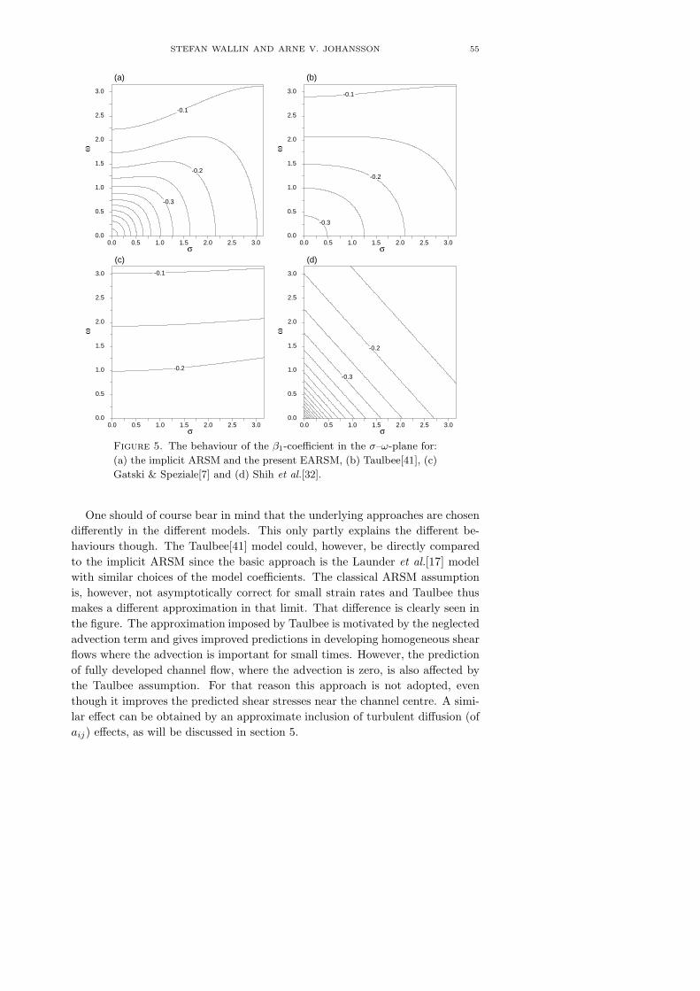
STEFAN WALLIN AND ARNE V. JOHANSSON 55
(a)
σ
ω
0.0 0.5 1.0 1.5 2.0 2.5 3.0 0.0
0.5
1.0
1.5
2.0
2.5
3.0
-0.1
-0.2
-0.3
(b)
σ
ω
0.0 0.5 1.0 1.5 2.0 2.5 3.0 0.0
0.5
1.0
1.5
2.0
2.5
3.0 -0.1
-0.2
-0.3
(c)
σ
ω
0.0 0.5 1.0 1.5 2.0 2.5 3.0 0.0
0.5
1.0
1.5
2.0
2.5
3.0 -0.1
-0.2
(d)
σ
ω
0.0 0.5 1.0 1.5 2.0 2.5 3.0 0.0
0.5
1.0
1.5
2.0
2.5
3.0
-0.2
-0.3
Figure 5. The behaviour of the β1-coefficient in the σ–ω-plane for:
(a) the implicit ARSM and the present EARSM, (b) Taulbee[41], (c)
Gatski & Speziale[7] and (d) Shih et al.[32].
One should of course bear in mind that the underlying approaches are chosendifferently in the different models. This only partly explains the different be-haviours though. The Taulbee[41] model could, however, be directly comparedto the implicit ARSM since the basic approach is the Launder et al.[17] modelwith similar choices of the model coefficients. The classical ARSM assumptionis, however, not asymptotically correct for small strain rates and Taulbee thusmakes a different approximation in that limit. That difference is clearly seen inthe figure. The approximation imposed by Taulbee is motivated by the neglectedadvection term and gives improved predictions in developing homogeneous shearflows where the advection is important for small times. However, the predictionof fully developed channel flow, where the advection is zero, is also affected bythe Taulbee assumption. For that reason this approach is not adopted, eventhough it improves the predicted shear stresses near the channel centre. A simi-lar effect can be obtained by an approximate inclusion of turbulent diffusion (ofaij) effects, as will be discussed in section 5.

56 AN EXPLICIT ALGEBRAIC REYNOLDS STRESS MODEL
The benefits of a direct, explicit solution of the production to dissipation ratiocan be further illustrated by considering rotating plane channel flow. The meanflow is here described by U (x2) δi1 and the system rotation is taken as ωsδi3.The mean strain rate tensor is unaffected by system rotation, implying that theeffective IIS for the calculation of P/ε is the same as for a non-rotating channelflow. The ‘effective’ second invariant of the mean rotation tensor (see equation(14)) becomes
IIRΩ = τ2
[−1
2(U ′)2 − 6
(134
)2
(ωs)2 + 2134ωsU ′
]. (28)
We note that, whereas the first two terms have the same sign on both sidesof the channel, the last term has an alternating sign. For moderate rotationrates the model will, thus, predict a decrease of P/ε on the side of the channelwhere IIΩ is increased, and vice versa. This is in agreement with the observedbehaviour of a stabilized and a destabilized side in rotating channel flow. Due tothe quadratic term (in ωs) in the expression for IIΩ the model will also predicta global decrease in P/ε for very large rates of rotation, as could be expectedfrom comparison with stability theory (see e.g. Matsson & Alfredsson[19]).
2.2. Solution of the simplified ARSM for three-dimensional mean flow.For general three-dimensional mean flows the solution for the β-coefficients canbe written as
β1 = −N(2N2 − 7IIΩ
)Q
, β3 = −12N−1IV
Q,
β4 = −2(N2 − 2IIΩ
)Q
, β6 = −6NQ
, β9 =6Q,
(29)
where all the other coefficients are identically zero. The denominator
Q =56(N2 − 2IIΩ
) (2N2 − IIΩ
)(30)
is also here clearly seen always to remain positive since IIΩ always is negative.The nonlinear equation for N or the corresponding equation for P/ε is for ex-
ample obtained by introducing the above solution (29) for a into the definitionof N . The resulting equation is of sixth order and reads
N6 − c′1N5 −(
2710IIS +
52IIΩ
)N4 +
52c′1IIΩN
3
+(II2Ω +
18920
IISIIΩ − 815V
)N2 − c′1II
2ΩN − 81
5IV 2 = 0. (31)
This equation reduces to the two-dimensional cubic equation by recalling that intwo-dimensional mean flows there are only two independent invariants, whereasIIIS = IV = 0 and V = IISIIΩ/2. Equation (31) cannot be solved in aclosed form but the solution of N for the cubic equation (25) applicable intwo-dimensional mean flow, Nc, can be used as a first approximation. A further

STEFAN WALLIN AND ARNE V. JOHANSSON 57
improvement of the approximation of N is also possible by making a perturba-tion solution of the three-dimensional equation. This is done by perturbing theIV and V invariants around the two-dimensional solution, that is IV =
√φ1 and
V = IISIIΩ/2 + φ2, assuming that φ1 and φ2 are independent. Putting this intothe three-dimensional equation (31) and sorting in powers of φ1 and φ2 we get
N = Nc +162(φ1 + φ2N
2c
)D
+ O (φ21, φ22, φ1φ2) (32)
where the denominator, D, is given by
D = 20N4c
(Nc − 1
2c′1
)− IIΩ
(10N3
c + 15c′1N2c
)+ 10c′1II
2Ω (33)
where (25) has been used to rewrite the expression for D. From (33) it is obviousthat D will always remain positive, since Nc ≥ c′1 (see Appendix C).
One could also consider keeping P/ε or N implicit during the iteration pro-cedure to a steady-state solution and thus avoid any further approximations.It is, however, not known how this would affect the stability of the numericalmethod and should be avoided. There could also be problems associated withthe existence of multiple roots, especially for three-dimensional cases.
2.2.1. Example of a three-dimensional mean flow: rotating pipe. Fully devel-oped turbulent flow in a circular pipe rotating around its length axis is an in-teresting case, since it represents a three-dimensional flow that can be describedwith only one spatial coordinate, r in a cylindrical coordinate system (r, θ, z).If the flow is laminar, the tangential velocity, Uθ, varies linearly with the radius,r, like a solid-body rotation. In turbulent flow, on the other hand, the tangentialvelocity is nearly parabolic, which cannot be described with an eddy-viscosityturbulence model. The fully three-dimensional form of the proposed EARSM isneeded to capture this behaviour. Limited forms with only second-order termsis not sufficient, as will be shown below.
The Navier–Stokes equation in the tangential direction can be written as
ν
(d2Uθ
dr2+
1r
dUθ
dr− Uθ
r2
)=
ddr
(Karθ) + 2Karθ
r. (34)
After two integrations, the tangential velocity can be expressed as
Uθ (r) = Uθ (R)r
R− r
ν
∫ R
r
Karθ
udu (35)
where R is the radius of the tube. The first term corresponds to the linear Uθ
profile while the second term is the correction that may give a parabolic-likeprofile if the arθ anisotropy is positive.

58 AN EXPLICIT ALGEBRAIC REYNOLDS STRESS MODEL
In this particular flow the strain- and rotation-rate tensors are evaluated inan inertial frame and read
S =12τ
0 dUθ
dr − Uθ
rdUz
drdUθ
dr − Uθ
r 0 0dUz
dr 0 0
(36)
and
Ω =12τ
0 −dUθ
dr − Uθ
r −dUz
drdUθ
dr + Uθ
r 0 0dUz
dr 0 0
. (37)
The terms that contribute to the arθ component in the general expression (18)are the terms associated with the β1, β5, β6 and β10-coefficients. In the case ofa linear Uθ profile, Srθ is zero and the contribution from the β1-term vanishes.This is consistent with the behaviour for an eddy-viscosity model.
We see from relation (35) that arθ should vanish rapidly for increasing Re. Toverify that the present EARSM is consistent with such a behaviour we start withthe EARSM solution for a flow that may deviate from solid-body rotation. Forthe present EARSM β5 and β10 are zero, which means that here only the linearterm (β1S) and the β6-term (associated with the
(SΩ2 +Ω2S− 2
3IV I)-group)
contribute to arθ:
arθ =12β1τ
(dUθ
dr− Uθ
r
)− 1
4β6τ
3
(dUθ
dr− Uθ
r
)(dUθ
dr+Uθ
r
)2
− 14β6τ
3 dUθ
dr
(dUz
dr
)2
. (38)
For solid body rotation only the third term remains and we see that the arθ
component will vanish only if the axial mean velocity gradient dUz/dr vanishes.This gradient does indeed vanish in the limit of infinite Reynolds number, butonly slowly1 with increasing Reynolds numbers while the relation (35) indicatesa more rapid decay rate (arθ → 1/Re).
The β1 and β6 coefficients in (38) are both negative, so the term with the axialmean velocity gradient (the last term) gives a positive contribution to arθ whichdrives the azimuthal velocity Uθ(r) towards a more parabolic-like profile (wheredUθ/dr > Uθ/r). The second term enhances this trend but what is interestingis that the β1-term (the first term) has the opposite sign and has the possibilityof balancing the arθ anisotropy component depending on the exact form of theβ-coefficients.
1The ‘two-layer hypothesis’ ⇒ (UCL − Uz)/uτ = f ((R − r)/R) ⇒(−(R/UCL)(dUz/dr))2 = (−(uτ /UCL)f
′)2 ∼ Cf where it is also well known that Cf
slowly decreases with increasing Reynolds number and that the mean velocity profile in a pipe
approaches a top-hat in the infinite Re limit (see e.g. Schlichting[30], chap. 20).

STEFAN WALLIN AND ARNE V. JOHANSSON 59
Hence, the required consistency of a rapidly vanishing arθ is indeed obtainedas a solution to the present EARSM, and is in fact associated with a non-zerodeviation from solid-body rotation for large but finite Reynolds numbers.
To clearly see this we may need to take a closer look at (38) by inserting thepresent EARSM solutions for β1, β6. This gives
arθ ∼(
7Uθ
r− dUθ
dr
)(dUz
dr
)2
−(
dUθ
dr− Uθ
r
)[814τ2
(C1 − 1 +
Pε
)2
+(
dUθ
dr+Uθ
r
)2]
(39)
and balance is obtained for a parabolic-like profile. Hence, the EARSM solutionimplies an anisotropy that vanishes much more rapidly than dUz/dr. As isobvious from (39) we also see that in the limit of infinite Re where dUz/dr → 0the vanishing arθ is associated with an EARSM solution that gives a solid-bodyrotation.
The rotation also affects the axial velocity component, which becomes less full,i.e. more parabolic. That effect enters mainly through the rotation dependencein the β1-coefficient and could thus be captured also by a linear eddy-viscositymodel where the Cµ-coefficient is dependent on the rotation rate.
A fully developed turbulent rotating pipe flow has been computed using theproposed model. The Reynolds number is 20 000 based on the mean flow ve-locity and tube diameter. Three different rotation ratios Z = 0, 0.5 and 1 werecomputed where Z = Uθ (R) /Um, i.e. the wall angular velocity divided by theaxial bulk velocity. The results are compared to the experiment by Imao, Itoh& Harada[14]. The turbulence models used are the Chien[1] K–ε model and theproposed EARSM including the near-wall formulation in section 3. The EARSMis based on both the K–ε and K–ω models discussed in section 3.4.
The three-dimensional form of the model has been used and the influence ofthe approximation of N was assessed by computing the case by using both thezeroth- (Nc) and first-order perturbation solution of N . The former is given by(26) and labelled ‘EARSM 0’ in the figures while the latter ‘EARSM 1’ is givenby (32).
Figure 6 shows the predicted axial velocity for Z = 1 using the Chien K–εmodel alone and as the platform for EARSM calculations. The original Chieneddy-viscosity K–ε model is seen to be completely insensitive to rotation, whilethe EARSM predictions agree well with the experimental results. It is alsoseen that the different approximations of N only have a minor influence on thepredicted velocity profile. In figure 7 predictions for different values of Z areshown for the K–ω model as the platform of the EARSM. The calculated resultsare seen to capture well the trend with increasing rate of rotation. The EARSMpredictions with the K–ε and K–ω platforms are quite similar except in a regionclose to the wall. The angular velocity (figure 8) is also seen to be reasonably well

60 AN EXPLICIT ALGEBRAIC REYNOLDS STRESS MODEL
r/R
U /
Uz
mea
n
0.0 0.2 0.4 0.6 0.8 1.0 0.0
0.4
0.8
1.2
1.6
Figure 6. Axial velocity in rotating pipe flow for rotation ratio
Z = 1. Computations with Chien K–ε model ( ) and the cur-
rent EARSM based on Chien K–ε, EARSM 0 ( ) and EARSM 1
( ), compared to experiment by Imao et al.[14] ( ).
predicted with the different EARSM formulations, among which the differencesare small.
The prediction of the velocity could, however, be improved by the inclusionof the neglected other cubic term associated with β5 (see (18)) and tuning thecoefficients for this special case, but it is worth noticing that the results here areobtained without any tuning whatsoever. Moreover, three-dimensional effectsdriven by turbulence are in most cases quite weak compared to three-dimensionaleffects driven by mean momentum forces. The rotating pipe is in this case veryextreme since the three-dimensional effects are purely turbulence driven.
The zeroth- and first-order solutions of N are only different approximationsof the exact solution for N or P/ε. The error can be investigated by computingthe P/ε ratio using the different approximations of N from a given flow field.Figure 9 shows P/ε with N evaluated from the first- (EARSM 0) and second-(EARSM 1) order solutions of N given by (26) and (32) respectively, comparedto the exact solution. The mean flow invariants of these expressions were takenfrom a fixed mean flow field, which was the solution with EARSM 0 based onK–ε for Z = 1. We can see a substantial difference between the zeroth- andfirst-order solutions and also that the first-order solution is quite close to theexact one. As seen from the previous figures this difference has still a quitesmall influence on the computed velocity profiles.
2.3. Solution of the general quasi-linear ARSM equation. So far, theexplicit solution of the ARSM resulting from the special case of the Launder etal.[17] model with c2 = 5/9 has been analysed. The solution procedure describedin this section can, however, be applied to any ARSM that has been derived froma linear or quasi-linear pressure–strain model. Quasi-linear here means that the

STEFAN WALLIN AND ARNE V. JOHANSSON 61
r/R
U /
Uz
mea
n
0.0 0.2 0.4 0.6 0.8 1.0 0.0
0.4
0.8
1.2
1.6
Figure 7. Axial velocity in rotating pipe flow for different rotation
ratios. Computations with the current EARSM (EARSM 0) based
on K–ω (lines) compared to experiment by Imao et al.[14] (symbols)
for Z = 1 ( ) ( ), Z = 0.5 ( ) ( ) and Z = 0 ( ) ( ).
r/R
U /
Uw
all
θ
0.0 0.2 0.4 0.6 0.8 1.0 0.00
0.20
0.40
0.60
0.80
1.00
Figure 8. Angular velocity in rotating pipe flow for rotation ratio
Z = 1. Computations with Chien K–ε model ( ) and the current
EARSM based on Chien K–ε, EARSM 0 ( ) and EARSM 1 ( ),
and the current EARSM (EARSM 0) based on K–ω ( ) compared
to experiment by Imao et al.[14] ( ).
pressure–strain model must be tensorially linear in a but may contain terms liketraSa. The resulting ARSM may be written
Na = −A1S+ (aΩ−Ωa) −A2
(aS+ Sa− 2
3traS
)(40)
where
N = A3 + A4Pε. (41)
The solution of (40) for three-dimensional mean flow was first derived byGatski & Speziale[7] where they considered the production to dissipation ratio

62 AN EXPLICIT ALGEBRAIC REYNOLDS STRESS MODEL
r/R
P/ε
0.0 0.2 0.4 0.6 0.8 1.0 0.00
0.50
1.00
1.50
2.00
Figure 9. Production to dissipation ratio in rotating pipe flow for
different approximation levels for N : EARSM 0 ( ) and EARSM 1
( ) compared to the exact ( ) solution. The mean flow from the
EARSM 0 K–ε solution for Z = 1 was used.
as a universal constant which is equivalent to A4 = 0. The fully consistentsolution for two-dimensional mean flow was first derived by Girimaji[8, 9] wherethe production to dissipation ratio was obtained as part of the solution.
The solution of (40) for three-dimensional mean flow is given in Appendix C.The algebra in that case is considerably more complex than for the simplifiedARSM with c2 = 5/9. In this section we restrict our attention to two-dimensionalmean flow for which the solution for the β-coefficients is
β1 = −A1N
Q, β2 = 2
A1A2
Qand β4 = −A1
Q. (42)
The denominator
Q = N2 − 2IIΩ − 23A22IIS (43)
for this case consists of both positive and negative terms but it can be shownthat it is strictly positive due to the fact that N is a function of IIS and IIΩ (seeAppendix C).
The Launder et al.[17] model (LRR) is a special case with the A1 to A4 coef-ficients given in table 3. Also, the SSG model by Speziale, Sarkar & Gatski[39]may be expressed in this form if it is linearized according to Gatski & Speziale[7].The SSG pressure–strain model reads
Πε
= −(C1
2+C∗1
2Pε
)a+
(C3 − C∗
3
2
√IIa
)S
+C4
2
(aS+ Sa− 2
3traSI
)− C5
2(aΩ−Ωa) +
C2
4
(a2 − 1
3IIaI),(44)
STEFAN WALLIN AND ARNE V. JOHANSSON 63
where IIa = tra2 and the coefficients are
C1 = 3.4, C∗1 = 1.8, C2 = 4.2, C3 =
45, C∗
3 = 1.30, C4 = 1.25, C5 = 0.40.
(45)
The linearized SSG model used by Gatski & Speziale[7] is then obtained byneglecting the quadratic anisotropy term and for the IIa invariant they used theequilibrium value predicted by the SSG model for two-dimensional homogeneousturbulence. This results in the following set of coefficients:
C1 = 3.4, C∗1 = 1.8, C2 = 0, C3 = 0.36, C∗
3 = 0, C4 = 1.25, C5 = 0.40,(46)
and A1 to A4 are given in table 3. Gatski & Speziale[7] based their EARSMon this linearized SSG pressure–strain model and implied an additional approx-imation in order to avoid the nonlinearity in the ARSM equation system. Theapproximation was to use the asymptotic value for the production to dissipationratio as a universal constant
Pε
=Cε2 − 1Cε1 − 1
(47)
which is equivalent to the A1 to A4-coefficients given in table 3 for Gatski &Speziale without regularization. The approximation made by Gatski & Speziale[7]is quite severe, especially since the A4-coefficient is zero which means that thedenominator Q given by (43) may become singular. However, in their final ex-pression they have regularized the denominator to avoid the singular behaviour.That form of the model, however, could not exactly be expressed through theA1 to A4-coefficients.
The predicted anisotropies in the log-layer and for the asymptotic homoge-neous shear flow are listed in tables 4 and 5. The linearized SSG model is ableto predict all individual Reynolds stresses fairly well for the two different cases.The Gatski & Speziale[7] model gives the same result for the asymptotic homo-geneous shear but fails in the log-layer since the approximation of the productionto dissipation ratio used by them is only consistent for asymptotic shear flows.It should be noted here that the regularization in the Gatski & Speziale modeldoes not influence the solution for these two cases.
The proposed model based on the LRR pressure–strain model is a reasonablechoice here due to its simplicity in three-dimensional mean flows, and since themost important anisotropies, namely a12 and a22, are fairly well predicted forboth the log-layer and for the asymptotic homogeneous shear flow. If betterpredictions of the a11 and a33 anisotropies are needed, the linearized SSG may beconsidered as an alternative but one should realize that this model is considerablymore complex for three-dimensional mean flows.

64 AN EXPLICIT ALGEBRAIC REYNOLDS STRESS MODEL
Table 3. The coefficients in the general ARSM for different models.
A1 A2 A3 A4
LRR 8815(7c2+1)
5−9c27c2+1
11(c1−1)7c2+1
117c2+1
Current model (c1 = 1.8, c2 = 5/9) 1.20 0 1.80 2.25Original LRR (c1 = 1.5, c2 = 0.4) 1.54 0.37 1.45 2.89linearized SSG 1.22 0.47 0.88 2.37Gatski & Speziale w/o regularization 1.22 0.47 5.36 0
Table 4. The predicted anisotropy in the log-layer using different
models assuming balance between turbulence production and dissi-
pation compared to channel DNS by Kim[16].
a12 a11 a22 a33 σ
DNS −0.29 0.34 −0.26 −0.08 1.65Current model (c1 = 1.8, c2 = 5/9) −0.30 0.25 −0.25 0.00 1.69Original LRR (c1 = 1.5, c2 = 0.4) −0.36 0.26 −0.20 −0.06 1.40Linearized SSG −0.32 0.36 −0.26 −0.10 1.59Gatski & Speziale w/o regularization −0.29 0.22 −0.16 −0.06 1.75Gatski & Speziale −0.28 0.22 −0.16 −0.06 1.76
Table 5. The predicted anisotropy in homogeneous shear flow us-
ing different models with σ = 3.0 compared to measurements by
Tavoularis & Corrsin[43].
a12 a11 a22 a33 P/εexpr −0.30 0.40 −0.28 −0.12 1.8Current model (c1 = 1.8, c2 = 5/9) −0.30 0.31 −0.31 0.00 1.8Original LRR (c1 = 1.5, c2 = 0.4) −0.38 0.32 −0.25 −0.07 2.3Linearized SSG −0.32 0.41 −0.30 −0.11 1.9Gatski & Speziale w/o regularization −0.32 0.41 −0.30 −0.11 1.9Gatski & Speziale −0.31 0.41 −0.30 −0.11 1.9
3. Near-wall treatments
In the model presented so far no special attention has been given to the verynear-wall region. To obtain the correct behaviour in this region it needs tobe modified in a similar way to low Reynolds number two-equation turbulencemodels. An important difference compared to eddy-viscosity models is that theeffective Cµ or β1 in the proposed model is not a constant and, as has beenshown by Wallin & Johansson[45], will adjust to the near-wall flow in a morenatural way than is possible with eddy-viscosity models.
STEFAN WALLIN AND ARNE V. JOHANSSON 65
The turbulence timescale τ = K/ε, which is used to scale the strain- androtation-rate tensors goes to zero as the wall is approached. A more appropriateexpression for the timescale was proposed by Durbin[4] and reads
τ = max(K
ε,Cτ
√ν
ε
). (48)
This is just the usual timescale with a lower bound given by the Kolmogorovscale. Durbin[4, 4] uses Cτ = 6.0 which will be kept in this study also.
In the very near-wall region of any shear flow the presence of the solid bound-ary will enforce a nearly parallel flow except in the immediate vicinity of a sepa-ration or stagnation point. A fully developed channel flow is exactly parallel andwill be used to formulate and calibrate the very near-wall correction. A specificcoordinate system will be used in the derivation of the near-wall correction butthe final form is invariant to coordinate system.
In a channel flow, as well as in all parallel flows, we can simply express theanisotropy in terms of the two-dimensional β-terms and the non-dimensionalshear, σ, which in parallel flow reads
σ =12K
ε
dUdy
. (49)
The invariants can then simply be expressed as IIS = 2σ2 and IIΩ = −2σ2 andthe anisotropy becomes
a12 = σβ1, a11 = σ2(
13β2 − 2β4
), a22 = σ2
(13β2 + 2β4
). (50)
By letting U in (49) represent the velocity along the limiting streamline atthe wall the expressions (50) can also be said to be approximately valid forthree-dimensional near-wall boundary layer flows.
The very near-wall behaviour is studied by using channel DNS data by Kim[16]at Reδ ≈ 7800 or Reτ ≈ 395. The mean velocity, K and ε profiles obtained fromthe DNS data have been used to compute the modelled anisotropy, which iscompared to the anisotropy determined directly from the DNS data.
The near-wall asymptotic behaviour can be written as
u+rms = auy+ + buy
+2 + · · · ,v+rms = avy
+2 + bvy+3 + · · · ,
w+rms = awy
+ + bwy+2 + · · · ,
K+ = aKy+2 + bKy
+3 + · · · ,−uv+ = auvy
+3 + buvy+4 + · · · .
(51)
So, Lai & Zhang[36] summarize these near-wall asymptotic coefficients, au, av, ...,for different experimental and numerical near-wall turbulence studies of flatplates, channels and pipes at different Reynolds numbers. These coefficientstogether with the DNS data by Kim[16] have been used to calibrate the coeffi-cients in the near-wall corrections.

66 AN EXPLICIT ALGEBRAIC REYNOLDS STRESS MODEL
3.1. The shear component of the Reynolds stress. In a channel flow, themean flow is only directly affected by the Reynolds shear stress, uv, so let usstart by looking at the model of a12.
The modelled a12 anisotropy without any near-wall corrections is nearly con-stant as the wall is approached while DNS data exhibit a behaviour similar to anexponential decay (see figure 10). The obvious choice of ‘wall damping function’is of van Driest type
f1 = 1 − exp(− y+
A+
). (52)
Also shown in figure 10 is the a12 behaviour predicted by a standard K–εmodel, without any near-wall damping function, which gives strongly negativevalues near the wall, almost down to −2. Note that this is well outside the rangeof physically realizable values, that are limited to be between ±1. The K–εmodel cannot be correctly damped towards the wall as easily as the EARSMand the EARSM is therefore much better suited to be integrated down to thewall. This is due to the fact that the β1 coefficient is not a constant, as in theeddy-viscosity hypothesis, but a function of the mean flow strain rate. In thevery near-wall region the strain, normalized by the turbulent timescale, becomeslarge but the β1-coefficient goes to zero for large strain rates giving a balanceda12 anisotropy (cf. figure 4).
The slope of the a12 anisotropy at the wall can be evaluated from the near-wall asymptotic behaviour to be da12/dy+ = −auv/aK . The constant A+ variesbetween 18 and 37 in the data summarized by So et al.[36]. By choosing A+ = 26,which also is the standard value in the van Driest function, a good fit to theDNS data is obtained according to figure 10, which shows the corresponding uv
Reynolds stress. The low Reynolds number coefficient can now be determinedas
β1,low-Re = f1β1, (53)
where β1 is the high Reynolds number coefficient obtained from the solution insection 2.
3.2. The normal components of the Reynolds stress. The correct near-wall behaviour for the normal Reynolds stresses is then ensured through a correctbehaviour of the β2- and β4-coefficients. The near-wall asymptotic behaviour ofthe a11 and a22 anisotropy is
a11 =u2
K− 2
3=
au2
aK− 2
3+ O (y+) ,
a22 =v2
K− 2
3=
av2
aKy+
2 − 23
= −23
+ O(y+
2). (54)

STEFAN WALLIN AND ARNE V. JOHANSSON 67
y+
a 12
0. 20. 40. 60. 80. 100. 120. 140. -0.35
-0.30
-0.25
-0.20
-0.15
-0.10
-0.05
0.00
y+
uv
0. 20. 40. 60. 80. 100. 120. 140. -1.05
-0.90
-0.75
-0.60
-0.45
-0.30
-0.15
0.00
Figure 10. a12 anisotropy (left) and uv stress (right) in channel
flow. Comparison of the current EARSM with near-wall correction
( ) with DNS data ( ) by Kim[16]. The computed a12 anisotropy
using the current EARSM without near wall correction ( ) and the
eddy-viscosity model ( ) is also shown. The predicted anisotropy
was evaluated by use of the DNS data for the S and Ω fields.
The modelled a11 and a22 anisotropies, without any wall corrections, are lim-ited near the wall, so a blending of the near-wall asymptote and the outer solutioncan be done. For simplicity, the same blending function, f2, is used for the bothanisotropies, which become
a11,low-Re = f2a11 + (1 − f2)(B2 − 2
3
),
a22,low-Re = f2a22 + (1 − f2)(−2
3
), (55)
where B2 = au2/aK . Equation (54) states that a22 has zero slope at the wall
so the function f2 must also have zero slope. A simple choice that satisfies thiscriterion is f2 = f1
2. The low Reynolds number coefficients then become
β2,low-Re =3B2 − 4
2σ2(1 − f1
2), β4,low-Re = f1
2β4 − B2
4σ2(1 − f1
2), (56)
where β4 is the high Reynolds number coefficient obtained from the solution insection 2.
The constant B2 can be evaluated using the data summarized by So et al.[36]and varies between 1.56 and 1.84. By choosing B2 = 1.8 a good fit to the DNSdata is obtained (see figures 11 and 12).
3.3. Extension to general flows. The near-wall correction described so farwas obtained for a special case, namely parallel two-dimensional flows, and can-not directly be generalized to three-dimensional mean flows. Some singulari-ties in flows near separation must be considered and the formulation needs tobe written in a coordinate-system-invariant form. These additional extensions

68 AN EXPLICIT ALGEBRAIC REYNOLDS STRESS MODEL
y+
a 11
0. 20. 40. 60. 80. 100. 120. 140. 0.0
0.2
0.4
0.6
0.8
1.0
1.2
1.4
y+
a 22
0. 20. 40. 60. 80. 100. 120. 140. -0.7
-0.6
-0.5
-0.4
-0.3
-0.2
-0.1
0.0
Figure 11. a11 (left) and a22 (right) anisotropies in channel flow.
Comparison of the current EARSM with ( ) and without ( )
near-wall correction with DNS data ( ) by Kim[16]. The predicted
anisotropy was evaluated by use of the DNS data for the S and Ω
fields.
y+
uu
0. 20. 40. 60. 80. 100. 120. 140. 0.0
1.5
3.0
4.5
6.0
7.5
9.0
10.5
y+
vv a
nd w
w
0. 20. 40. 60. 80. 100. 120. 140. 0.0
0.5
1.0
1.5
2.0
2.5
3.0
3.5
Figure 12. Reynolds stresses in channel flow. Comparison of the
current EARSM, u2 ( ) (left) and v2 ( ), w2 ( ) (right),
with DNS data, ( ) and ( ) by Kim[16]. The predicted anisotropy
was evaluated by use of the DNS data for the S and Ω fields.
must be formulated such that the original form above is retained for paralleltwo-dimensional flows.
So far, the near-wall correction is described in terms of σ, which is defined in(49) for a specific coordinate system. By using IIS = 2σ2, a coordinate-system-invariant form of the near wall correction can be obtained. In separated flowthe shear rate σ may become small, leading to a singular behaviour of the nearwall corrections to the β2- and β4-coefficients. To avoid this problem, the shearrate in the denominator of the near-wall correction is limited to the equilibriumshear rate where the turbulence production balances the dissipation rate. The

STEFAN WALLIN AND ARNE V. JOHANSSON 69
near-wall shear rate is always larger than the equilibrium one in zero pressuregradient flows and the limiter will only be active in flows near separation. Theanisotropy model including the near-wall formulation then reads
a = f1β1S+(1 − f1
2) 3B2 − 4
max (IIS , IIeqS )
(S2 − 1
3IIS I
)+(f1
2β4 −(1 − f1
2) B2
2 max (IIS , IIeqS )
)(SΩ−ΩS) (57)
where IIeqS is the equilibrium value obtained by setting P = ε in the two-dimensional solution and reads IIeqS = 405c21/ (216c1 − 160) ≈ 5.74 for c1 = 1.8.The β-coefficients are given by equation (24) and f1 is given by equation (52).Please observe that even though the high Reynolds number β2-coefficient is zerothe tensor group associated with the β2-coefficient does not vanish.
The straightforward extension to three-dimensional flow reads
a = f1β1S+(1 − f1
2) 3B2 − 4
max (IIS , IIeqS )
(S2 − 1
3IIS I
)+ f21β3
(Ω2 − 1
3IIΩ I
)+(f1
2β4 −(1 − f1
2) B2
2 max (IIS , IIeqS )
)(SΩ−ΩS)
+ f1β6
(SΩ2 +Ω2S− 2
3IV I
)+ f21β9
(ΩSΩ2 −Ω2SΩ
)(58)
This form reduces to (57) for two-dimensional mean flows.The near-wall correction is strictly valid only for parallel two-dimensional
mean flow but the very near-wall flow is, however, near parallel and two-dimen-sional also for quite complex three-dimensional flow fields so the equation (58)can be used as a first approximation. The correction can be extended to also bevalid for flows near stagnation points like separation and reattachment points,for flows over curved surfaces and also for three-dimensional mean flows. Thisextension of the near-wall correction is, however, outside the scope of this paperbut will be addressed in future studies.
3.4. Lengthscale determining equation. So far, we have proposed a newexplicit constitutive relation between the mean flow strain rate and the Reynoldsstresses including near-wall treatments. The choice of velocity- and length-scaledetermining equations has not yet been discussed. The turbulent kinetic energy,K, is a natural choice for determining the turbulent velocity-scale since thisequation needs no further modelling. The dissipation of the turbulent kineticenergy, ε, is the most commonly used quantity for determining the turbulentlength-scale but other alternatives are also possible like τ and ω.
Common to all length-scale determining equations is that they need a lotof ad hoc modelling, substantially more than the K-equation. The differentterms are quite empirical and are tuned for specific flow cases. There are manydifferent K–ε models with the major differences in the near-wall modelling in

70 AN EXPLICIT ALGEBRAIC REYNOLDS STRESS MODEL
the ε-equation and in the eddy-viscosity relation. Most of the ε-models are alsotuned and calibrated together with the eddy-viscosity assumption, which givesa poor description of the near-wall anisotropy. One should thus not be surprisedif the proposed EARSM together with an existing length-scale model does notgive any improvements and perhaps also worse capabilities in predicting basicwall-bounded flows.
The correct methodology to obtain a length-scale determining equation is todevelop it from scratch together with the proposed EARSM, so that one avoidsthe risk of inheriting terms that are needed to balance the errors introduced bythe eddy-viscosity assumption. This is, however, outside the scope of this paperbut will be addressed in future studies. For an illustration of the capability ofthe proposed model and to obtain an indication of how different length-scaledetermining equations act, we have tested the proposed model together with thewell known Chien[1] K–ε model and the Wilcox[48] K–ω model for the fullydeveloped channel case simulated by Kim[16].
In these computations we did not use the Daly & Harlow model, equation (17),of the diffusion terms in the K and ε (or ω) equations. The approach was to usethe standard eddy-viscosity modelling of the diffusion term but with an effectiveCµ evaluated from the EARSM such as Ceff
µ = −f1β1/2. The differences betweenthe Daly & Harlow and the eddy-viscosity approaches were found to be smallfor the K–ε model as long as the effective Cµ is used rather than a constant. Incase of the K–ω model, the turbulent diffusion is complete different comparedto that of the K–ε model and thus the Daly & Harlow approach needs to berecalibrated. The eddy-viscosity approach could, however, directly be used alsohere as long as the effective Cµ (or β∗) is used. In three-dimensional mean flowsthe effective Cµ is Ceff
µ = −f1(β1 + IIΩβ6)/2Figures 13 to 18 show the result of the computations with the two different
two-equation models based on the proposed EARSM as well as with the originaleddy-viscosity assumption. The EARSM has been used both with the originaland modified (‘mod’) length-scale equations.
If we first look at the velocity profiles in figure 13 one finds that the additiveconstant B in the log-law is much too high when the EARSM is used. Thisclearly illustrates the need for recalibration discussed above. The figure alsoshows the results when the length-scale equation is tuned or modified to bettermatch the log-law. In the K–ε model the definition of ε in Chien’s model hasbeen changed to
ε = ε +2νKy2
exp(−Cky
+), (59)
where the constant Ck = 0.04. This means that the original ‘wall dissipation’ ismultiplied by an exponential function to give a more rapid decay of the modifi-cation near the wall. In the Wilcox K–ω model, the constant Rβ was increased

STEFAN WALLIN AND ARNE V. JOHANSSON 71
log y+
U+
0.0 1.0 2.0 3.0 0.0
8.0
16.0
24.0
log y+
U+
0.0 1.0 2.0 3.0 0.0
8.0
16.0
24.0
Figure 13. The streamwise velocity in channel flow. Computations
based on Chien K–ε (left) and K–ω (right) using eddy-viscosity ( )
and the current EARSM with the original ( ) and modified ( )
ε and ω equations compared with DNS data ( ) by Kim[16] and the
log-law ( ).
y+
k+
0. 40. 80. 120. 0.0
2.0
4.0
6.0
y+
k+
0. 40. 80. 120. 0.0
2.0
4.0
6.0
Figure 14. The turbulent kinetic energy in channel flow. Computa-
tions based on Chien K–ε (left) and K–ω (right) using eddy-viscosity
( ) and the current EARSM with the original ( ) and modified
( ) ε and ω equations compared with DNS data ( ) by Kim[16].
from 8 to 10 to obtain the desired behaviour. For a more thorough comparisonbetween K–ε and K–ω models the reader may wish to consult Menter[21].
It is also interesting to note the clear improvement in the K-profiles with theproposed EARSM both for the K–ε and K–ω models in figure 14. The near-wall dissipation ratio shown in figure 15 illustrates the need for a better near-wallmodelling of the length-scale equation. In figures 16 to 18 we can see the goodnear-wall behaviour of the proposed EARSM which seems to be quite insensitiveto the choice of basic two-equation model. In figure 16 we can also clearly seehow poorly the a12 anisotropy is predicted with the eddy-viscosity models.

72 AN EXPLICIT ALGEBRAIC REYNOLDS STRESS MODEL
y+
ε+
0. 40. 80. 120. 0.00
0.08
0.16
0.24
y+
ε+
0. 40. 80. 120. 0.00
0.08
0.16
0.24
Figure 15. The dissipation of turbulent kinetic energy in channel
flow. Legend as in figure 14.
y+
a 12
0. 40. 80. 120. -0.3
-0.2
-0.1
0.0
y+
a 12
0. 40. 80. 120. -0.3
-0.2
-0.1
0.0
Figure 16. The a12 anisotropy in channel flow. Legend as in figure 14.
y+
uv+
0. 40. 80. 120. -1.2
-0.8
-0.4
0.0
y+
uv+
0. 40. 80. 120. -1.2
-0.8
-0.4
0.0
Figure 17. The uv Reynolds stress in channel flow. Legend as in
figure 14.

STEFAN WALLIN AND ARNE V. JOHANSSON 73
y+
uu+
and
vv+
0. 40. 80. 120. 0.0
2.0
4.0
6.0
8.0
y+
uu+
and
vv+
0. 40. 80. 120. 0.0
2.0
4.0
6.0
8.0
Figure 18. The normal Reynolds stresses in channel flow. Legends
as in figure 14.
The rotating pipe flow discussed in section 2.2.1 was computed with thesetwo models (K–ε and K–ω) as platforms for EARSM. Figures 6 and 7 show thatdifferences are seen in a region close to the wall, where the K–ε based modelshows a higher wall shear stress than the K–ω based model. The latter correctlycaptures the trend of a decreasing skin friction with increasing rate of rotation,whereas the K–ε based EARSM gives the opposite trend.
3.5. Alternative near-wall scaling. The damping function, f1 given by equa-tion (52), is formulated in terms of y+. The scaling with the local wall skin fric-tion is not valid in flows near separation and reattachment. Other possibilitiesthan y+ are Rey ≡ √
Ky/ν or the turbulent Reynolds number Ret ≡ K2/νε (seee.g. Wilcox[47]).
The approach is here to formulate an alternative scaling y∗ in terms of Rey orRet so that y∗ ≈ y+ for y+ ≤ 100 in channel flows. Rey and Ret were computedfrom DNS data at different Reynolds numbers ranging from Reτ = 150 to 650 inchannel flows (Moser, Kim & Mansour[22]) and zero pressure gradient boundarylayers (Spalart[37]). It was found that Rey was increasing from the wall morelinearly with less scattering compared to Ret. Moreover, it should not poseany major problems to compute the wall distance y needed for Rey if that isdefined as the distance to the closest wall point. The following form for y∗ isthus proposed:
y∗ = Cy1
√Rey + Cy2Re
2y. (60)
The√Rey-term is motivated by the fact that the near-wall asymptotic behaviour
for Rey is ∼ y2. The Re2y-term is artificially introduced to obtain a near linearrelation in the buffer region also. With Cy1 = 2.4 and Cy2 = 0.003 good agree-ment with y+ for channel and zero pressure gradient boundary layer flows atdifferent Reynolds numbers is obtained, see figure 19.

74 AN EXPLICIT ALGEBRAIC REYNOLDS STRESS MODEL
y+
y*
0. 50. 100. 150. 0.
50.
100.
150.
y+
f1
0. 50. 100. 150. 0.00
0.40
0.80
1.20
Figure 19. (left) The near-wall scaling y∗ compared to y+. (right)
The damping function f1 using y∗ or y+. The original form using y+
( ) is compared to channel DNS data (Moser et al.[22]) at different
Reynolds numbers Reτ = 180, 395 and 590 ( ) and zero pressure
gradient boundary layer DNS data (Spalart[37]) at Reτ = 150, 325
and 650 ( ). y∗ increases with increasing Reynolds number.
In the damping function f1, y+ is then replaced by y∗
f1 = 1 − exp(− y∗
A+
). (61)
In figure 19 the damping function f1 based on y∗ is compared to f1 based ony+. The correspondence is good except for the lowest Reynolds numbers.
In some situations the y+ scaling may worsen the computational results. Ina forthcoming study by M. Skote adverse pressure gradient boundary layers arestudied by DNS. For the highest pressure gradient studied, with the pressuregradient similarity parameter m = −0.25 (U∞ ∼ xm), the difference betweenthe y+ and y∗ approaches are significant here, see figure 20. For this case it isobvious that the y+ scaling degenerates the model performance and should beavoided.
In other cases, where the Reynolds number is higher, the near-wall scaling isnot as critical. Figure 21 shows the computational results for the two-dimensionalRAE2822 aerofoil profile using the proposed EARSM compared to the Wilcox[48]K–ω model. The flow in this case is compressible and the formulation is modifiedin a manner described in section 4. The EARSM approach clearly improves theposition of the shock and the results are very much in line with differentialReynolds stress computations by Hellstrom, Davidsson & Rizzi[12] for exactlythe same conditions and geometry.
The damping function in the EARSM is formulated in terms of y+ as wellas y∗ and the figure shows no major differences between these approaches ex-cept in the separated region where the y+ formulation gives a somewhat largernegative skin friction. In the figure a computation using the proposed EARSM

STEFAN WALLIN AND ARNE V. JOHANSSON 75
X
Cf
150. 200. 250. 300. 350. 0.000
0.001
0.002
0.003
0.004
U
y
0.00 0.25 0.50 0.75 0.0
10.0
20.0
30.0
Figure 20. (left) The wall skin friction and (right) the velocity pro-
file for an adverse pressure gradient boundary layer (U∞ ∼ x−0.25).
Computations with standard Wilcox[46] K–ω ( ), Chien K–ε
( ), EARSM based on K–ω and y+ ( ) or y∗ ( ) and the
Hanjalic[11] RST model ( ). Comparisons with DNS data ( ),
Skote (private communication).
without any damping functions whatsoever is also shown. For that choice, thestandard Wilcox[46] K–ω, also without damping functions, must be used as theplatform. This combination gives, however, incorrect near-wall behaviour for theturbulence quantities but the mean velocity profiles are well reproduced. Thatis also seen in the figure where no major differences between the EARSM withor without damping functions are present.
The convergence history is shown in figure 22 where we can see that thereare no major differences in convergence rate. Actually, the proposed EARSMconverges to a somewhat lower residual than the corresponding eddy-viscositymodel for this case. The numerical parameters are the same for these two casesand the computational time for the 5000 iteration steps is 6% higher for theEARSM computation. This case was found to be not completely numericallystationary which results in the residual ‘hanging’ as for the K–ω model. Thefluctuations are, however, very small and could not be seen in the solution. Inother cases without separation the convergence curves are even closer to eachother, and the convergence rates are in general faster than for the case shownin figure 22. The computational results were obtained using the EURANUScode[25] which is an explicit time-stepping multigrid and multiblock Navier–Stokes solver. The grid convergence was assessed by repeating the computationon a coarser grid.
A further example is a three-dimensional transonic supercritical wing (figure23). This case is computed using the standard Wilcox[46] K–ω model and theEARSM based on that. Since that K–ω model has no damping functions theEARSM without damping functions must also be used for consistency. Again,

76 AN EXPLICIT ALGEBRAIC REYNOLDS STRESS MODEL
x/c
Cp
0.00 0.20 0.40 0.60 0.80 1.00 1.00
0.50
0.00
-0.50
-1.00
-1.50
x/c
Cf
0.00 0.20 0.40 0.60 0.80 1.00 -0.006
-0.002
0.002
0.006
0.010
Figure 21. Wall pressure and skin friction coefficients for the
RAE2822 wing profile (M = 0.754, α = 2.57 and Re = 6.2 · 106).
Predictions using Wilcox[48] K–ω ( ) and the current EARSM
based on K–ω with damping function based on y+ ( ), y∗ ( )
or without any damping functions ( ), compared to experimental
data ( ) (Cook et al.[2]). The geometry is the measured one including
a camber correction.
iter
rho_rms
0. 2000. 4000. 6000. -6.0
-4.0
-2.0
0.0
Figure 22. Convergence history for the RAE2822 wing profile.
Wilcox K–ω ( ) compared with the current EARSM based on
K–ω ( ). The computational time is increased by 6% by using
EARSM. Three levels of full multigrid is used.
the predicted shock position is improved compared to the eddy-viscosity model.This case illustrates the benefit of the proposed model which is also viable in ex-pensive three-dimensional cases, here with almost one million grid points. Mostimportantly, there is no substantial increase in the computational cost comparedto the, in many cases, robust standard K–ω model.

STEFAN WALLIN AND ARNE V. JOHANSSON 77
x/c
Cp
0.00 0.25 0.50 0.75 1.00 1.00
0.20
-0.60
-1.40
Figure 23. Wall pressure coefficient Cp for the LANN-wing (M =
0.82, α = 2.59 and Re = 5.4×10⁶) at the spanwise position of 0.474.
Predictions using Wilcox[46] K–ω ( ) and the current EARSM
( ) based on K–ω without wall damping functions. Comparison
with experimental data ( ) (Horsten et al.[13]).
4. Compressibility
Many turbulent flow applications are within the Mach number regime wherecompressible effects must be considered. Also, in low speed flow compressible ef-fects may be important due to local heating or cooling of the flow. Compressibleturbulent flow may be classified according to Friedrich[6] into flows with van-ishing compressibility effects due to turbulent fluctuations and flows where sucheffects play a significant role. Friedrich[6] also states that compressibility effectsdue to turbulent fluctuations might be important in hypersonic, high Mach num-ber, wall-bounded flows and in mixing layers at high convective Mach numbers.The understanding of such flows is poor and models capable of distinguishing theprincipal differences between wall-bounded and free shear flows are not well de-veloped. The compressibility effects, due to turbulent fluctuations, increase theanisotropy of the Reynolds stress tensor (see Friedrich[6]) and depend themselveson the anisotropy, which means that algebraic Reynolds stress models are bettersuited than eddy viscosity models to act as a basis for improving the predictionof compressibility effects.
In wall-bounded flows with Mach numbers below 5 compressibility effects dueto turbulent fluctuations may be neglected and the effect of compressibility entersinto the problem essentially only through the mean flow compressibility. In thisstudy we will restrict the attention to this class of flows and a straightforwardcompressibility extension of the incompressible model will be made.
First, the stress anisotropy and the turbulent kinetic energy must be redefinedas aij ≡ ρuiuj/ρK−2δij/3 and K ≡ ρuiui/2ρ where ρ is the local mean densityof the fluid. The trace of the strain is not zero for compressible flow. We may

78 AN EXPLICIT ALGEBRAIC REYNOLDS STRESS MODEL
instead use a somewhat redefined normalized strain rate tensor
Sij ≡ τ
2(Ui,j + Uj,i) − D
3δij , (62)
where the normalized dilatation of the mean flow is defined as D ≡ τUk,k.The redefinition of S to have zero trace allows us to make use of the in-
compressible solution process. The redefinition also implies, however, that theS33-component is non-zero for two-dimensional mean flow in the (x, y)-plane andthat the simplifications for two-dimensional mean flow are not strictly valid forcompressible flow. This will be addressed as a special case later in this section.
The general linear model of the LRR rapid pressure–strain rate model forincompressible flow does not have zero trace in compressible flow, so the modelneeds to be generalized according to Vandromme[44] and reads
Π(r)ij = −c2 + 8
11
(Pij − 2
3Pδij
)− 30c2 − 2
55ρK
(Ui,j + Uj,i − 2
3Ul,lδij
)− 8c2 − 2
11
(Dij − 2
3Pδij
)(63)
where Pij = −ρuiukUj,k − ρujukUi,k and Dij = −ρuiukUk,j − ρujukUk,i. Theincompressible models for the slow pressure–strain and the dissipation tensor canalso be used here. The general ARSM for compressible flow can now be writtenas (
c1 − 1 − 6c2 + 411
D − traS)a = − 8
15S+
7c2 + 111
(aΩ−Ωa)
− 5 − 9c211
(aS+ Sa− 2
3traSI
)(64)
which is identical to the incompressible form, equation (13), except for the di-latation term 0n the left-hand side and the different definitions given above. Thesame conclusion is valid for the simplified equation obtained by setting c2 = 5/9,which reads (
c1 − 1 − 23D − traS
)a = − 8
15S+
49
(aΩ−Ωa) . (65)
The solution of the simplified compressible ARSM equation is the same as theincompressible solution except for the definition of the c′1-coefficient, which forthe compressible case is
c′1 =94
(c1 − 1 − 2
3D)
(66)
bearing in mind that Sij here is defined by (62).

STEFAN WALLIN AND ARNE V. JOHANSSON 79
4.1. Compressible two-dimensional mean flow. An approximation of thecompressible ARSM equation can be derived by an expansion around a so-lution obtained by use of the two-dimensional simplification valid in incom-pressible flow. Let us first define a compressible two-dimensional strain rateas S2D
ij ≡ (τ/2) (Ui,j + Uj,i)−Dδ2Dij /2 where δ2Dij ≡ δij except that δ2D33 = 0. Thecompressible ARSM, equation (65), can now be written as(
c1 − 1 − 23D − tra2DS2D
)a2D = − 8
15S2D +
49(a2DΩ−Ωa2D
)(67)
with the solution a2D, which is derived using the two-dimensional solution pro-cess for incompressible flow. The true anisotropy, a, is then related to the solu-tion a2D, as described below.
The difference between S and S2D is of O (D) which can be assumed smallexcept in a shock wave. For the same reason the difference between a and a2D
can also be assumed to be of O (D) and with the simplest tensorial form thatrelates the two-dimensional and three-dimensional anisotropies, leading to thefollowing assumption. Let
a = a2D + βaD(I2D − 2
3I)
+ O (D2), (68)
and subtract equation (67) from equation (65). Sorting terms in powers of Dgives us the first-order solution in D
βa = − 415 (c1 − 1 − tra2DS2D)
. (69)
In obtaining this solution the following relations have been used:
S2D = S− D2
(I2D − 2
3I)
tra2DS2D = traS + O (D2)
(70)
a2DΩ−Ωa2D = aΩ−Ωa+ O (D2).
The zeroth-order solution, a2D, is obtained as described for the incompressiblecase, with the only difference being that c′1 is now given by (66). The full solutionis then given by
a = β1S2D + β4(S2DΩ−ΩS2D
)+ βaD
(I2D − 2
3I)
+ O (D2)
(71)
with βa from (69).
4.2. Shock/boundary layer interaction. The compressible form of the pro-posed model together with the near-wall formulations has been tested on ashock/boundary layer interaction. A turbulent boundary layer at Mach 5 ona flat plate interacts with an oblique shock from a shock generator above theplate, see figure 24. The flow deflection angle is 10 which gives a strong enough

80 AN EXPLICIT ALGEBRAIC REYNOLDS STRESS MODEL
999999999999999999999999999999999999999999999999999999999999999999999999
99999999999999999999999999999999999999999999999999999999999999999999999999999999
999999
Expansion fan
Shock generator
Incoming shock Reflected shock
InteractionBoundary layer
Computationaldomain
Figure 24. Impinging shock at Mach 5. Experimental and compu-
tational setup.
shock to cause a boundary layer separation. The experiment by Schulein, Krog-mann & Stanewsky[29] was performed at DLR in Gottingen. Figure 25 showsthe computed wall pressure and skin friction coefficient along the flat plate com-pared to the experimental data. The turbulence models used are the Chien[1]K–ε model and the Wilcox[48] K–ω model based on the original eddy-viscosityassumption and also based on the proposed EARSM. The computational resultswere obtained using the EURANUS code[25]. The grid convergence was assessedby repeating the computation on a coarser grid.
The size of the separated region is underestimated by the two eddy viscos-ity models whereas a correct separation length is obtained when the models arebased on the proposed EARSM. This can be seen both in the skin friction be-haviour and in the wall pressure distribution. The computed wall pressure is,however, somewhat shifted downstream.
The Chien K–ε model strongly over-predicts the skin friction downstreamof the reattachment point, which is typical for many low Reynolds number K–εmodels. This behaviour is inherited by the proposed EARSM based on the ChienK–ε model. The K–ω models give much better skin friction predictions.
5. Diffusion term
In regions of the flow where the production to dissipation ratio is small, theassumption of negligible effects of advection and diffusion of the anisotropy maycause problems, also noticed by Taulbee[41]. In the outer-most part of a bound-ary layer and in the centre of a turbulent channel flow the magnitude of the β1coefficient may thus be too large leading to an overestimation of the uv Reynoldsstress. The behaviour of the model can be analysed by looking at the effectiveCeff
µ ≡ −β1/2 when the strain rate goes to zero, which for the simplified ARSMreads
Ceffµ (σ → 0) =
35c′1
. (72)
For the proposed model constants Ceffµ ≈ 0.33 which is far too high.

STEFAN WALLIN AND ARNE V. JOHANSSON 81
x [m]
P w
all [
kPa]
0.30 0.36 0.42 0.48 0.
15.
30.
45.
x [m]
Cf
0.30 0.36 0.42 0.48 -0.002
0.002
0.006
0.010
Figure 25. (left) Wall pressure and (right) skin friction coefficient
for the impinging shock at Mach 5 with the flow deflection angle
β = 10. Comparison of the predictions using Chien K–ε ( ),
Wilcox K–ω ( ) and the current EARSM based on K–ε ( )
and K–ω ( ) with the experiment by Schulein et al.[29] ( ).
In this section we will discuss the possibility of including a correction to theARSM equations formulated so that the proposed EARSM solution process canbe retained. The transport equation for the Reynolds stress anisotropy is givenby (1) where Tijl and T
(K)l are the flux terms for the Reynolds stress tensor and
turbulent kinetic energy. A simple model for the neglected diffusion term maybe written as
∂Tijl
∂xl− uiuj
K
∂T(K)l
∂xl= CDaij
∂T(K)l
∂xl, (73)
which gives a modification of the c′1-coefficient in the simplified ARSM equation(21). The modified coefficient reads
c′1 =94
(c1 − 1 − CD
ε
∂T(K)l
∂xl
). (74)
There are, however, numerical problems associated with this form due to theinclusion of the second derivative of K. This could be avoided if the term thatbalances the turbulent flux term in the K-equation (15) is used to approximatethe turbulent flux of K:
∂T(K)l
∂xl≈ P − ε. (75)
The advection of K is neglected here. Moreover, the extra term worsens themodel behaviour for large strain rates and can even lead to a singular behaviour.The correction thus needs to be switched off for P/ε > 1. The definition of the

82 AN EXPLICIT ALGEBRAIC REYNOLDS STRESS MODEL
c′1-coefficient then becomes
c′1 =94
[c1 − 1 + CD max
(1 − P
ε, 0)]
. (76)
The problem with this form is that it is implicit in the P/ε ratio and that themax function makes it impossible to solve. The diffusion model will thus befurther approximated by using P/ε = −β1IIS . If β1 is approximated with βeq1where P = ε, the correction is guaranteed to be zero in the log-layer and forhigher strain rates. The definition of the c′1-coefficient now becomes
c′1 =94
[c1 − 1 + CD max (1 + βeq1 IIS , 0)] (77)
where
βeq1 = −65
N eq
(N eq)2 − 2IIΩ(78)
and
N eq =9c14. (79)
The constant CD can now be estimated by looking at the effective Cµ forzero strain rates in (72). With CD = 2.2 the effective Cµ becomes Ceff
µ = 0.09which is close to what one should expect. The a12 anisotropy with the proposeddiffusion model is compared to the basic EARSM in figure 26 for parallel flow(cf. figure 4). The inclusion of the diffusion model makes the proposed EARSMbehave almost the same as the SST model for this case. In figure 27 we can seean improvement of the a12 anisotropy prediction near the centre of the channelsimulated by Kim[16]. The actual difference in the predicted mean velocityprofile is quite small. This improvement is similar in character to that obtainedby the correction introduced by Taulbee[41] although the two approaches aremotivated differently.
The derivation of the diffusion correction is based on a number of ad hocarguments and should be seen only as a possible extension of the model to flowsituations where diffusion may be of substantial importance.
6. Concluding remarks
For two-dimensional mean flows the new proposed EARSM represents an exactsolution of the implicit ARSM relation for the anisotropy tensor, but also a goodapproximation for three-dimensional mean flows. The fact that it fully accountsfor three-dimensional effects gives it a natural predictive capability for complexflows. This was demonstrated here by capturing the correct trends for axiallyrotating pipe flow. Standard two-equation models predict a solid-body rotationwith an unaffected axial velocity profile. In reality the azimuthal velocity hasa variation that is close to parabolic and the rotation causes the axial velocityprofile to be less full, i.e. more parabolic. To capture these features the modeldescription of the inter-component transfer is crucial. For instance, the simplified

STEFAN WALLIN AND ARNE V. JOHANSSON 83
σ
a 12
hom. shear
log-layer
0.0 0.5 1.0 1.5 2.0 2.5 3.0 -0.6
-0.5
-0.4
-0.3
-0.2
-0.1
0.0
Figure 26. The a12 anisotropy versus strain rate σ for parallel flow.
The current model without ( ) and with ( ) diffusion model
compared to an eddy-viscosity model ( ) and the Menter[20] SST
model ( ).
y+
a 12
0. 100. 200. 300. 400. -0.35
-0.30
-0.25
-0.20
-0.15
-0.10
-0.05
0.00
Figure 27. The a12 anisotropy in channel flow. Comparison of the
current EARSM without ( ) and with ( ) diffusion model with
the eddy-viscosity model ( ) and DNS data ( ) by Kim[16].
linear rapid pressure–strain model of Launder et al.[17] and Naot, Shavit &Wolfstein[23], usually referred to as the isotropization of production model, doesnot have the necessary ingredients. The full linear model, on the other hand,together with linear models for the other terms, was demonstrated here to besufficient to capture the main features of the flow in the axially rotating pipe.In general the predictive capability of the proposed EARSM for rotating flowsis substantially better than standard two-equation models and than EARSMformulations including only terms up to second order in S and Ω.
The extension to compressible flows is done in a simple way in the presentEARSM in which the equations are expressed by use of Favre averages. Com-pressibility of the mean flow is accounted for, but no explicit compressibility

84 AN EXPLICIT ALGEBRAIC REYNOLDS STRESS MODEL
corrections are added to the ‘platform’ (K–ε, K–ω . . . ) equations. With someminor redefinitions the same ARSM relation for aij as for incompressible flowcould be used also here. This approach for wall-bounded turbulent flows is ad-equate for Mach numbers up to about 5. It was shown to capture the essentialfeatures of the complex interaction between an inclined shock and a turbulentboundary layer at Mach 5. In particular it describes the skin friction and sep-aration length much better than standard two-equation models. Compared tothe standard two-equation models on which the present EARSM is based it alsogives a substantial improvement for the prediction of the skin friction variation inincompressible boundary layers with adverse pressure gradient (detailed resultsnot reported here).
Poor prediction of the effects of rotation and the under-prediction of separa-tion tendency in adverse pressure gradient boundary layers are well known defi-ciencies of closures based on the eddy-viscosity hypothesis. The present EARSMsubstantially improves these two aspects, and reduces the need for wall damping.A simple way to obtain the correct near-wall limits of the anisotropies was con-structed here on the basis of a van Driest type of damping function. For channelflow this was shown to give a very accurate description, and a simple method toretain numerical stability for situations with separated flows was demonstrated.A form of wall damping function based on Rey ≡ √
Ky/ν was shown to be anattractive alternative to forms based on y+ in flows with (or near) separation.
The reduced need for wall damping is coupled to the fact that the presentEARSM automatically predicts a production to dissipation ratio with correctasymptotic behaviour for large strain rates. For instance, in parallel flows thiscorrectly gives an asymptotically constant shear stress anisotropy componentfor large strains (shear rates). This behaviour is not a natural part of eddy-viscosity based models, but was incorporated in a somewhat ad hoc manner byMenter[21]. In the present model this behaviour emanates naturally from theunderlying modelling of the terms in the RST equations and the direct solutionof the production to dissipation ratio.
To further illustrate the behaviour for large strain rates the proposed modelwas tested in homogeneous shear flow at high initial shear rate. The good predic-tions that was obtained for this case can, however, be regarded as a bit fortuitousin the light of the fact that the basic ARSM approximation is somewhat ques-tionable for a case with a significantly non-zero left-hand side of the aij transportequation (∂aij/∂t = 0). Moreover, the Launder et al.[17] model does not giveaccurate predictions of this case when used in a differential form. It is, however,a fact that the self-consistent approach (i.e where the production to dissipationratio is solved for as part of the total EARSM-solution) gives a model with thecorrect asymptotic behaviour, which is a pre-requisite for reasonable predictionsin the limit of high shear. The present model is not constructed specifically to

STEFAN WALLIN AND ARNE V. JOHANSSON 85
incorporate such effects. It is, however, an important step towards a more gen-eral engineering model that the model is also able to give reasonable results inextreme flow cases.
Perhaps the most important feature of the proposed model is the numeri-cal behaviour. The computational cost is not significantly increased comparedto standard eddy-viscosity two-equation models and the general numerical be-haviour is almost the same. Implementation of this model into flow solvers withexisting eddy-viscosity two-equation models should not pose major problems.The model may be formulated in terms of an effective eddy viscosity with anadditional correction that may be treated fully explicitly (see Appendix A).
The authors would like to thank Dr Torbjorn Sjogren and Dr Magnus Hallbackfor many helpful discussions, especially concerning the treatment of rotating co-ordinate systems. The first author would also like to thank Dr Sharath Girimajifor many helpful discussions, especially concerning non-equilibrium turbulence.The authors gratefully acknowledge funding of this study from the EuropeanSpace Agency within a project for improving the modelling of turbulent flowsrelated to hypersonic lifting vehicles and would like to acknowledge Dr IngemarLindblad for leading this project.
Appendix A. Summary of the proposed model
The Reynolds stresses may be written in terms of an effective Cµ-coefficientwhich is mathematically identical with the formulation in section 2:
uiuj = K
(23δij − 2Ceff
µ Sij + a(ex)ij
), (80)
where the effective Cµ-coefficient is
Ceffµ = −1
2f1 (β1 + IIΩβ6) , (81)
and the extra anisotropy a(ex)ij then becomes
a(ex) =(1 − f1
2) 3B2 − 4
max (IIS , IIeqS )
+ f21β3
(Ω2 − 1
3IIΩ I
)(S2 − 1
3IIS I
)+(f1
2β4 −(1 − f1
2) B2
2 max (IIS , IIeqS )
)(SΩ−ΩS)
+ f1β6
(SΩ2 +Ω2S− IIΩS− 2
3IV I
)+ f21β9
(ΩSΩ2 −Ω2SΩ
). (82)
Here a, S and Ω denote second rank tensors, tr denotes the trace and I isthe identity matrix. The inner product of two matrices is defined as (SS)ij ≡(S2)ij
≡ SikSkj . The normalized mean strain and rotation tensors are defined

86 AN EXPLICIT ALGEBRAIC REYNOLDS STRESS MODEL
as
Sij =τ
2(Ui,j + Uj,i) , Ωij =
τ
2(Ui,j − Uj,i) , (83)
where the turbulent timescale is defined by
τ = max(K
ε,Cτ
√ν
ε
). (84)
The invariants are defined by
IIS = trS2, IIΩ = trΩ2, IV = trSΩ2, V = trS2Ω2, (85)
and
IIeqS =405c21
216c1 − 160. (86)
By introducing an effective Cµ-coefficient one can easily introduce this levelof modelling into flow solvers with existing two-equation eddy-viscosity modelsby setting
νt = Ceffµ Kτ. (87)
The contribution from the extra anisotropy a(ex)ij may now be added as fully
explicit additional terms in the equations.The β-coefficients are given by
β1 = −N(2N2 − 7IIΩ
)Q
, β3 = −12N−1IV
Q,
β4 = −2(N2 − 2IIΩ
)Q
, β6 = −6NQ
, β9 =6Q,
(88)
with the denominator
Q =56(N2 − 2IIΩ
) (2N2 − IIΩ
). (89)
For most purposes it is sufficient to take N = Nc where
Nc =
c′13
+(P1 +
√P2
)1/3+ sign
(P1 −
√P2
)| P1 −
√P2 |1/3, P2 ≥ 0
c′13
+ 2(P 21 − P2
)1/6cos
(13
arccos
(P1√
P 21 − P2
)), P2 < 0
(90)
with
P1 =
(c′1
2
27+
920IIS − 2
3IIΩ
)c′1, P2 = P 2
1 −(c′1
2
9+
910IIS +
23IIΩ
)3
(91)
and
c′1 =94
(c1 − 1) . (92)
An additional term can be added to Nc in order to improve the accuracy forthree-dimensional mean flows (see section 2.2).

STEFAN WALLIN AND ARNE V. JOHANSSON 87
The simplifications for two-dimensional mean flow are
β1 = −65
Nc
N2c − 2IIΩ
, β4 = −65
1N2
c − 2IIΩ, β3 = β6 = β9 = 0. (93)
The damping function reads
f1 = 1 − exp(−C′
y1
√Rey − C′
y2Re2y
), (94)
where
Rey =√Ky
ν. (95)
Finally, the five model constants are
Cτ = 6.0, c1 = 1.8, B2 = 1.8, C′y1 =
2.426.0
, C′y2 =
0.00326.0
. (96)
Appendix B. The completeness of the a(S,Ω) expression with tenterms
Based on the derivations of Spencer & Rivlin[38] for matrix polynomials Pope[24]concluded that there are ten independent terms in the complete expressiona(S,Ω). One should here restrict the meaning of independence to polynomialindependence as was also pointed out by Taulbee, Sonnenmeier & Wall[42]. Thehighest-order term
(ΩS2Ω2 −Ω2S2Ω
)in expression (18) is of order 5 and ex-
tension 3.The S and Ω tensors can appear in powers up to 2. A term SmΩn is then
said to be of power m + n and extension 2, etc. Shih & Lumley[34] (see alsoShih[33]) also include a term of power 6 and extension 4. They use a notationwith the mean velocity gradient tensor and its transpose, but with the presentnotation such a term can be written as
SΩ2S2Ω−ΩS2Ω2S− 23VI I, (97)
where the invariant VI equals trSΩ2S2Ω. One may first note that the invariantVI is of third power in Ω, which means that it cannot be expressed in terms of apolynomial in the other invariants, which are of order zero or two in Ω. Hence,VI contains sign information that is not contained in the other invariants. Wecan derive the following relation for its square:
VI2 =IIΩ
3
144(9IIS3 + 2IIIS2
)+IIΩ
2
6(−3V IIS2 + IV IIS IIIS
)+IIΩ8(10V 2IIS − 4V IV IIIS − IV 2IIS
2)− V 3 +
12V IV 2IIS − 1
3IV 3IIIS .
In the present modelling the invariant VI will not appear since it would arisefrom the product of the highest (fifth-order) term and S, and even in the generalsolution (for c2 = 5/9) the coefficient β10 = 0.

88 AN EXPLICIT ALGEBRAIC REYNOLDS STRESS MODEL
We can furthermore express the sixth-order term as the following combinationof lower-order terms
SΩ2S2Ω−ΩS2Ω2S− 23VI I =
(23V +
112IISIIΩ
)(SΩ−ΩS)
+ 13IV
(S2Ω−ΩS2
)− 16IIΩ
(SΩS2 − S2ΩS
)+ 1
6IIS(ΩSΩ2 −Ω2SΩ
).
By use of the generalized Cayley–Hamilton theorem it is fairly straightforwardto show that no other independent sixth- or higher-order term exists (see e.g.Shih & Lumley[34].
Appendix C. Solution of the general quasi-linear ARSM equation
The implicit general quasi-linear ARSM equation is rewritten similarly to thesimplified equation (21)
Na = −A1S+ (aΩ−Ωa) −A2
(aS+ Sa− 2
3traS
), (98)
where
N = A3 + A4Pε. (99)
The simplified equation is now a special case of (98) with the coefficients A1 =6/5, A2 = 0, A3 = c′1 and A4 = 9/4. For the general case we require that A1,A3 and A4 are positive.
C.1. Solution for two-dimensional mean flow. The solution for two-dimensionalmean flow is
β1 = −A1N
Q, β2 = 2
A1A2
Q, β4 = −A1
Q, (100)
where the denominator
Q = N2 − 2IIΩ − 23A22IIS . (101)
The equation for N is, for two-dimensional mean flow,
N3 −A3N2 −((
A1A4 +23A22
)IIS + 2IIΩ
)N + 2A3
(13A22IIS + IIΩ
)= 0,
(102)
with the solution
N =
A3
3+(P1 +
√P2
)1/3+ sign
(P1 −
√P2
)| P1 −
√P2 |1/3, P2 ≥ 0
A3
3+ 2(P 21 − P2
)1/6cos
(13
arccos
(P1√
P 21 − P2
)), P2 < 0
(103)
where
P1 =(A3
2
27+(A1A4
6− 2
9A2
2
)IIS − 2
3IIΩ
)A3 (104)

STEFAN WALLIN AND ARNE V. JOHANSSON 89
and
P2 = P 21 −
(A3
2
9+(A1A4
3+
29A2
2
)IIS +
23IIΩ
)3
. (105)
Let us investigate whether the denominator in equation (101) can becomezero. Equation (102) can be rewritten, by using equation (101), as
Q (N −A3) = A1A4IISN, (106)
which shows that Q > 0 if N > A3. The problem is then to show that N > A3.Let us first look at the special case when IIS = 0. Equation (102) can then bewritten
(N −A3)(N2 − 2IIΩ
)= 0, (107)
with the only real root N = A3. Differentiating equation (102) with respect toIIS gives
∂N
∂IIS=
23A
22 (N −A3) + A1A4N
3(N − 2
3A3
)N − (A1A4 + 2
3A22
)IIS − 2IIΩ
, (108)
which is positive if N ≥ A3. When IIS = 0 (108) can be written as
∂N
∂IIS
∣∣∣∣IIS=0
=A1A3A4
A23 − 2IIΩ
> 0. (109)
So far we know that N = A3 for IIS = 0 and that N increases until (108) changessign. By using (102) IIΩ can be eliminated in (108) which then becomes
∂N
∂IIS=
23A
22 (N −A3)
2 + A1A4N (N −A3)
2N (N −A3)2 + A1A3A4IIS
. (110)
From this form it is obvious that the denominator is strictly positive and that∂N/∂IIS = 0 for IIS = 0 only (where N = A3). Hence, the numerator is strictlypositive and N increases for all IIS , showing that N ≥ A3 for all IIS . Thecorresponding relation for the simplified ARSM equation is N ≥ c′1.
The denominator Q is thus always positive which guarantees a non-singularsolution.
C.2. Solution for three-dimensional mean flow. The solution of the linearequation system where N is assumed as known can be formulated as (see Gatski& Speziale[7])
Nβλ = −A1δ1λ +∑γ
Jλγβγ −A2
∑γ
Hλγβγ (111)
or in the standard form for linear equation systems
(Nδγλ − Jγλ + A2Hγλ)βλ = −A1δ1γ (112)

90 AN EXPLICIT ALGEBRAIC REYNOLDS STRESS MODEL
where the matrixes are given below for three-dimensional mean flow
H =
0 13IIS − 2
3IIΩ 0 0 23IV − 1
3V 0 0 02 0 0 0 0 2IIΩ IV 0 0 00 0 0 0 0 IIS
13IIIS 0 0 0
0 0 0 0 12IIS 0 0 1
3IIIS −IV − 13V − 1
6IISIIΩ0 0 0 1 0 0 0 0 −IIΩ − 2
3IV
0 0 1 0 0 0 12IIS 0 0 0
0 0 0 0 0 −1 0 0 0 00 0 0 0 −1 0 0 0 0 1
3IIΩ0 0 0 0 0 0 0 0 0 − 1
3IIS0 0 0 0 0 0 0 0 −2 0
,
(113)
J =
0 0 0 −IIΩ 0 0 0 2V − IISIIΩ II2Ω 00 0 0 0 −IIΩ 0 0 −2IV 0 II2Ω0 0 0 0 −2IIS 0 0 0 −2IV 2IISIIΩ − 2V1 0 0 0 0 1
2IIΩ 0 0 0 00 1 0 0 0 0 1
2IIΩ 0 0 00 0 0 3 0 0 0 IIS −2IIΩ 00 0 0 0 3 0 0 0 0 −2IIΩ0 0 0 0 0 0 0 0 0 00 0 0 0 0 −1 0 0 0 00 0 0 0 0 0 −1 0 0 0
.
(114)
The solution for three-dimensional mean flow is
β1 = −12A1N
(30A2IV − 21NIIΩ − 2A2
3IIIS + 6N3 − 3A22IISN
)/Q,
β2 = −A1A2
(6A2IV + 12NIIΩ + 2A2
3IIIS − 6N3 + 3A22IISN
)/Q,
β3 = −3A1
(2A2
2IIIS + 3NA2IIS + 6IV)/Q,
β4 = −A1
(2A2
3IIIS + 3A22NIIS + 6A2IV − 6NIIΩ + 3N3
)/Q,
β5 = 9A1A2N2/Q,
β6 = −9A1N2/Q,
β7 = 18A1A2N/Q,
β8 = 9A1A22N/Q,
β9 = 9A1N/Q,
β10 = 0, (115)
References 91
with the denominator
Q = 3N5 +(− 15
2IIΩ − 7
2A2
2 IIS
)N3 + ( 21A2 IV −A2
3 IIIS )N2
+ ( 3 IIΩ2 − 8 IIS IIΩA22 + 24A2
2 V + A24 IIS
2 )N +23A2
5 IIS IIIS
+ 2A23 IV IIS − 2A2
3 IIΩ IIIS − 6 IV A2 IIΩ. (116)
By substituting N = 1, A1 = 1 and A2 = 1 one gets the same ARSM equationas Gatski & Speziale[7] and also an identical solution.
The equation for N can also be derived for three-dimensional mean flow andis a sixth order polynomial equation, as for the simplified case. The expressionis, however, complicated and of small practical interest. As for the solution ofthe simplified ARSM equation, the two-dimensional solution of N can also beused here as a first approximation.
References
[1] Chien, K.Y. 1982 Predictions of channel and boundary-layer flows with alow-Reynolds-number turbulence model. AIAA J. 20, 33–38.
[2] Cook, P.H., MacDonald, M.A. & Firmin, M.C.P. 1979 Aerofoil 2822- Pressure distributions, boundary layer and wake measurements. AGARD AR138.
[3] Daly, B.J. & Harlow, F.H. 1970 Transport equations in turbulence. Phys.Fluids 13, 2634–2649.
[4] Durbin, P.A. 1993 Application of a near-wall turbulence model to boundarylayers and heat transfer. Int J. Heat Fluid Flow 14, 316–323.
[5] Durbin, P.A. 1995 Separated flow computations with the K–ε–v2 model.AIAA J. 33, 659–664.
[6] Friedrich, R. 1996 Compressibility effects due to turbulent fluctuations.Oral presentation at Sixth European Turbulence Conference, Lausanne, July1996, submitted to Journal of Appl. Sci. Res.
[7] Gatski, T.B & Speziale C.G. 1993 On explicit algebraic stress models forcomplex turbulent flows. J. Fluid Mech. 254, 59–78.
[8] Girimaji, S.S. 1996 Fully-explicit and self-consistent algebraic Reynoldsstress model Theor. and Comp. Fluid Dyn. 8 387–402 (also ICASE ReportNo. 95-82).
[9] Girimaji, S.S. 1996 Improved algebraic Reynolds stress model for engineer-ing flows In Engineering Turbulence Modelling and Experiments 3 pp 121–129.Eds W. Rodi and G. Bergeles. Elsevier. Science B.V.
[10] Girimaji, S.S. 1997 A Galilean invariant explicit algebraic Reynolds stressmodel for turbulent curved flows Phys. Fluids. 9 1067–1077 (also ICASE ReportNo. 96-38).

92 References
[11] Hanjalic, K., Jakirlic, S. & Hadzic, I. 1995 Computation of oscillatingturbulent flows at transitional Re-numbers Turbulent Shear Flows 9 pp 323–342. Eds F. Durst, N. Kasagi & B.E. Launder. Springer-Verlag, Berlin.
[12] Hellstrom, T., Davidson, L. & Rizzi, A. 1994 Reynolds stress trans-port modelling of transonic flow around the RAE2822 airfoil. AIAA 94-030932nd Aerospace Sciences Meeting, Reno, Jan 1994.
[13] Horsten, J.J., den Boer, R.G. & Zwaan, R.J. 1983 Unsteady tran-sonic pressure measurements on a semi-span wind tunnel model of a transport-type supercritical wing (LANN model). AFWAL-TR-83-3039.
[14] Imao, S., Itoh, M. & Harada, T. 1996 Turbulent characteristics of theflow in an axially rotating pipe J. Heat Fluid Flow 17, 444–451.
[15] Johansson, A.V. & Wallin, S. 1996 A new explicit algebraic Reynoldsstress model. Proc. Sixth European Turbulence Conference, Lausanne, July1996, Ed. P. Monkewitz, 31–34.
[16] Kim, J. 1989 On the structure of pressure fluctuations in simulated turbu-lent channel flow. J. Fluid Mech. 205, 421–451.
[17] Launder, B.E., Reece, G.J. & Rodi, W. 1975 Progress in the develop-ment of a Reynolds-stress turbulence closure. J. Fluid Mech. 41, 537–566.
[18] Lumley, J.L. 1978 Computational modeling of turbulent flows. Adv. Appl.Mech. 18, 123–176.
[19] Matsson, O.J.E. & Alfredsson, P.H. 1990 Curvature- and rotation-induced instabilities in channel flow. J. Fluid Mech. 210, 537–563.
[20] Menter, F.R. 1993 Zonal Two Equation K–ω Turbulence Models for Aero-dynamic Flows. AIAA 93-2906
[21] Menter, F.R. 1994 Two-equation eddy-viscosity turbulence models forengineering applications. AIAA J. 32, 1598–1604.
[22] Moser, R.D, Kim J. & Mansour N.N. 1998 DNS of Turbulent ChannelFlow up to Reτ = 590. Phys. Fluids 11, 943–945.
[23] Naot, D., Shavit, A. & Wolfstein, M. 1973 Two-point correlationmodel and the redistribution of Reynolds stresses. Phys. Fluids 16, 738–743.
[24] Pope, S.B. 1975 A more general effective-viscosity hypothesis J. FluidMech. 72, 331–340.
[25] Rizzi, A., Eliasson, P., Lindblad, I., Hirsch C., Lacor, C.,
Haeuser, J. 1993 The engineering of multiblock/multigrid software for Navier–Stokes flows on structured meshes Computers Fluids 22, 341–367.
[26] Rodi, W. 1972 The prediction of free turbulent boundary layers by use ofa two equation model of turbulence. Ph.D. thesis, University of London.
[27] Rodi, W. 1976 A new algebraic relation for calculating the Reynoldsstresses. Z. angew. Math. Mech. 56, T219–221.
[28] Rotta, J.C. 1951 Statistische Theorie nichthomogener Turbulenz. Z. Phys.129, 547–572.
[29] Schulein, E., Krogmann, P. & Stanewsky, E. 1996 Documentation

References 93
of Two-Dimensional Impinging Shock/ Turbulent Boundary Layer InteractionFlow. DLR Report: DLR IB 223 - 96 A 49.
[30] Schlichting, H. 1979 Boundary-Layer Theory, 7th ed., McGraw-Hill, NewYork.
[31] Shabbir, A. & Shih, T.H. 1992 Critical Assessment of Reynolds StressTurbulence Models Using Homogeneous Flows NASA TM 105954, ICOMP-92-24, CMOTT-92-12.
[32] Shih, T.H., Zhu, J. & Lumley, J.L. 1992 A Realizable Reynolds StressAlgebraic Equation Model NASA TM 105993, ICOMP-92-27, CMOTT-92-14.
[33] Shih, T.-H. 1996 Constitutive relations and realizability of single-point tur-bulence closures Chapter 4 of Turbulence and Transition Modelling, Eds.M. Hallback, D.S. Henningson, A.V. Johansson and P.H. Alfredsson. Kluwer.
[34] Shih, T.-H. & Lumley, J.L. 1993 Remarks on turbulent constitutiverelations Math. Comput. Modelling, 18, 9–16.
[35] Sjogren, T. 1997 Development and Validation of Turbulence ModelsThrough Experiment and Computation Doctoral thesis, Dept. of Mechanics,KTH, Stockholm, Sweden.
[36] So, R.M.C., Lai, Y.G. & Zhang, H.S. 1991 Second-Order Near-wallTurbulence Closures: A Review. AIAA J. 29, 1819–1835.
[37] Spalart P.R. 1988 Direct simulation of a turbulent boundary layer up toRθ = 1410. J. Fluid Mech. 187, 61–98.
[38] Spencer, A.J.M. & Rivlin, R.S. 1959 The theory of matrix polynomialsand its application to the mechanics of isotropic continua Arch. Rat. Mech.Anal. 2, 309–336.
[39] Speziale, C.G., Sarkar, S. & Gatski, T.B. 1991 Modelling thepressure–strain correlation of turbulence: an invariant dynamical systems ap-proach. J. Fluid Mech. 227, 245–272.
[40] Speziale, C.G. & Xu, X.-H. 1996 Towards the development of second-order closure models for nonequilibrium turbulent flows Int. J. Heat and FluidFlow 17, 238–244.
[41] Taulbee, D.B. 1992 An improved algebraic Reynolds stress model andcorresponding nonlinear stress model. Phys. Fluids A 4, 2555–2561.
[42] Taulbee, D.B., Sonnenmeier, J.R. & Wall, K.M. 1994 Stress relationfor three-dimensional turbulent flows Phys. Fluids 6, 1399–1401.
[43] Tavoularis, S. & Corrsin, S. 1981 Experiments in nearly homogeneousturbulent shear flow with a uniform mean temperature gradient. Part I. J. FluidMech. 104, 311–347.
[44] Vandromme, D. 1992 Introduction to the Modeling of Turbulence vonKarman Institute for Fluid Dynamics, Lecture Series 1991-02.
[45] Wallin, S. & Johansson, A.V. 1996 A new explicit algebraic Reynoldsstress turbulence model including an improved near-wall treatment. Proc.Flow Modeling and Turbulence Measurements VI, Tallahassee FL, Chen, Shih,

94 References
Lienau & Kung (eds), 399–406.[46] Wilcox, D.C. 1988 Reassessment of the scale-determining equation foradvanced turbulence models. AIAA J. 26, 1299–1310.
[47] Wilcox, D.C. 1993 Turbulence modeling for CFD. DCW Industries Inc.,La Canada, California.
[48] Wilcox, D.C. 1994 Simulation of transition with a two-equation turbu-lence model. AIAA J. 32, 247–255.

Paper 22


97
A PREDICTION METHOD FOR HIGH SPEED TURBULENT SEPARA-TED FLOWS WITH EXPERIMENTAL VERIFICATION
I. A. A. Lindblad (Head Comp. aerodynamics dept.), S. Wallin (Research Scientist)The Aeronautical Research Institute of Sweden (FFA), Bromma, Sweden
A. V. Johansson, (Professor)The Royal Institute of Technology (KTH), Stockholm, Sweden
R. Friedrich (Professor), R. Lechner (PhD student)Technische Universität München (TUM), Garching, Germany
P. Krogmann (Senior Research Scientist), E. Schülein (Research Scientist)Deutsches Zentrum für Luft- und Raumfahrt (DLR), Göttingen, Germany
J.-C. Courty (Senior Research Scientist), M. Ravachol (Research Scientist)Dassault Aviation (DAA), St Cloud, Paris, France
D. Giordano (ESA Technical Project Officer)ESA/ESTEC, Noordwijk, The Netherlands
Abstract. It is well known that the level of current engineering computationalaerodynamic analysis for turbulent hypersonic separated flows is not satisfactory.Computations using standard two-equation turbulence models do not give suffi-ciently accurate predictions. Existing compressibility corrections do not providegeneral improvements. In fact, they seem to render predictions worse, at least forMach numbers up to five. Possible improvements using Explicit Algebraic Turbu-lence Models (EARSM) have been investigated. This class of models allow for amore general coupling between the mean field and the turbulent Reynoldsstresses, compared to the standard two-equation models based on the Boussinesqhypothesis. A new class of EARSMs is proposed and compared to results of exist-ing standard models. It is demonstrated that the new proposed EARSM givesimproved prediction over standard two-equation models and previously publishedEARSMs for validation cases relevant for high speed separated flows. A newcomplete EARSM turbulence model based on the k-ω two-equation model is rec-ommended as giving the overall best prediction of the validation test cases. Aspart of the project a new series of detailed validation experiments, with turbulentboundary layer-shock wave interaction on a flat plate at Mach 5, with differentdegree of flow separation, have been performed.
1. Introduction
1.1. Problems in hypersonic aerodynamics. Future space transportation sys-tems, in particular reusable vehicles, will have to be more aerodynamically optimisedthan current designs. Currently novel space transportation concepts are under consider-ation, in Europe and elsewhere. The detailed evaluation of the technical feasibility andeconomy of the concepts as well as technical development of a selected design must be

98 PREDICTION METHOD, EXPR. VERIFICATION, HIGH SPEED TURBULENT SEPARATED FLOWS
done to a large extent by CFD methods, in part because full scale flight conditions can-not in general be reproduced in ground based experimental facilities.
External as well as internal flows are of importance. Heat loads of complex attachedand separated flows must be determined with sufficient accuracy. Current industrialstandard CFD methods in some cases fall short of supplying a reliable solution to thegiven analysis problem. In many instances the shortcomings are related to the turbu-lence modeling in Reynolds Averaged Navier-Stokes methods. In the current project wehave mainly dealt with the problem of predicting turbulent flow separation in high-speed flows. Typical applications are air intakes of hypersonic airbreathing vehicles orflow over control surfaces, with hinge line flow separation.
1.2. Project description. Turbulence modeling in high-speed flows is a vast subject.Our approach has been that a more general modeling, including the necessary flowphysics, will be able to treat a wider range of flow problems, also in areas of ’extrapola-tion’ beyond the regime of calibration of the model. With this general idea turbulencemodeling has been reviewed (Lindblad et al., 1995, chs 3-4). As a result of this review aclass of turbulence models, Explicit Algebraic Reynolds Stress Models (EARSMs) wasselected for further study and development.
The EARSM is formulated together with a base-line two equation turbulence model.In the project three partners (FFA, TUM, DAA) used different base-line models, whichwere all modified to be EARSM. To compare results and to judge the most promisingroute of development the codes were first tested on common schematic test cases (Wal-lin et al., 1996). In order to ensure that the codes gave the same results with the samemodels and assumptions, test cases assuming laminar flow or using a simple algebraicturbulence model were computed. The results using the different base-line models weresubsequently compared. All base-line models were modified, to include publishedEARSMs.
Based on the experiences of implementation and validation of existing EARSMs anew anisotropy formulation was developed (Johansson and Wallin, 1996; Wallin &Johansson, 1997). This model was implemented in the codes on the basis of the differ-ent two-equation turbulence models and tested. One variant was selected as giving theoverall best results.
A set of test cases was selected for the project, after an extensive review of suitableflow cases for the validation of turbulence models for the selected classes of targetproblems (Lindblad et al. 1995; Wallin et al. 1996). These were mainly schematic two-dimensional cases related to the selected target problems, used for model developmentand validation. A three-dimensional test case (Rodi & Dolling, 1992) was selected forthe demonstration of the generality of the model development and implementation.
One project goal was to contribute to the database of validation data for turbulencemodels at high speed. In the literature survey a lack of schematic test cases for hyper-sonic shock wave-turbulent boundary layer interaction was identified. A set of test

INGEMAR A. A. LINDBLAD ET AL. 99
experiments, with a shock wave incident on flat plate boundary layer at Mach 5 wasconducted by DLR (Krogmann & Schülein, 1996). This was used as the main valida-tion case in the project. The results are summarised in section 4.
Selected project computational results, demonstrating the main findings, are ana-lysed in section 5. The main conclusions of the turbulence model development and val-idation, as well as the lessons learned from the experimental campaign are summarisedin section 6.
2. Problems in turbulence modeling for high speed flows
2.1. The required level of modeling. In the review of turbulence modeling forhigh speed flows (Lindblad et al., 1995, ch. 4) the specific problems of turbulence mod-els for compressible flows were investigated. It was concluded that intrinsic compressi-bility effects on the turbulence had a significant influence on free shear flows. In wallbounded flows the main influence of compressibility (for Mach numbers less than five)lies in the interaction between the turbulence and the compressible mean field. Theimportance of the intrinsic compressibility effects on turbulence is measured by a tur-bulent Mach number. Recent evidence (Sarkar, 1995, Blaisdell et al. 1991) points to thegradient Mach number as the representative compressible parameter.Here S is the mean shear rate, λ is a representative integral length scale and c is themean speed of sound.
In cases where the turbulent Mach number (or gradient Mach number) is large,explicit compressibility terms should be added to the turbulence model equations.Attempts have been made at modeling pressure-dilatation correlation and dilatationaldissipation rate for compressible flows (e.g. Sarkar et al., 1991; Zeman, 1990). How-ever, these do in general not agree well with experimental or DNS results, in particularnot for wall-bounded flows.
As noted above the main target applications in the current project feature flow sepa-ration of wall bounded flows. We have concluded that the most fruitful direction ofdevelopment is to improve on incompressible turbulence models, formulated for com-pressible flow by applying Favre averaging to the equations. A survey of incompressi-ble turbulence models was performed, aimed at the question of prediction of separatedflows. It was concluded that in order to seek a general improvement in prediction of awide class of separated flows in complex configurations, it is necessary to work withReynolds Stress turbulence models. In general prediction of complex, separated flowsrequires a realistic model for the anisotropy of the Reynolds stress tensor, appearing inthe averaged Navier-Stokes equations. In principle it would be advantageous to derive atransport equation for the independent stress components, leading to a differential Rey-nolds Stress Model (DRSM). The practical application of DRSM is still in early stages.The implementation and calibration of DRSM models are quite complex for the typesof target problems envisioned for the current project. The computational cost and prob-
Mg S λ c⁄( )=

100 PREDICTION METHOD, EXPR. VERIFICATION, HIGH SPEED TURBULENT SEPARATED FLOWS
lems with numerical robustness precludes the use of DRSM models for engineeringpurposes in the near future.
In two-equation models the transport equations for individual Reynolds stresses arereplaced by a simple algebraic proportionality between the Reynolds Stress anisotropy,
and the mean flow strain rate (Boussinesq’s hypothesis). This is a quite simplis-tic model for the Reynolds stress components and is formally valid only for the shearstress component, uv, in near parallel flows in equilibrium. Despite this, the standardtwo-equation turbulence models work quite well in many engineering flow problems,attesting to the fact that these are often close to equilibrium. A possible route forimproving on the known deficiencies of two-equation models in prediction e.g. flowseparation, is to generalise the relation between the Reynolds stress anisotropy and themean flow strain and rotation rate
(1)
This is the idea of the Algebraic Reynolds Stress Models (ARSM), pioneered byRodi (1972, 1976). The first of these models were formulated as implicit relations to besolved as part of the iteration process. The use of ARSM has been slowed by thenumerical difficulties, as serious as for DRSMs, which are due to the implicit and non-linear algebraic relations to be solved in the ARSM case. This has motivated the devel-opment of Explicit Algebraic Reynolds Stress Models (EARSM) in which the Rey-nolds Stress anisotropy is expressed as an explicit function of the mean flow strain androtation rate tensors,
. (2)
The EARSM formulation allows a direct evaluation of the Reynolds stress termsonce the mean field is known. This is quite amenable to the numerical procedures offlow solvers and makes EARSM models as robust as two-equation turbulence models.
2.2. Development of an EARSM anisotropy model. In the current projectEARSMs have been reassessed and a novel development has been made. Publishedmodels (Shih, Zhu & Lumley, 1992; Gatski & Speziale, 1993) were implemented andtested for reference. The EARSM concept has been reassessed and a new model devel-oped (Johansson & Wallin, 1996; Wallin & Johansson, 1996). The following maindevelopments have been made.• The development of the complete explicit expression from (2) in terms of a
series of nonlinear combinations of and . The coefficients of this series havebeen determined to make the EARSM anisotropy model an exact solution of theARSM equations for two-dimensional flows and an approximate solution for three-dimensional flows.
aij Sij
f aij Sij, Ωij,( ) 0=
aij aij Sij Ωij,( )=
aijSij Ωij

INGEMAR A. A. LINDBLAD ET AL. 101
• A calibration of the near wall behaviour of the new EARSM. A low Reynoldsnumber formulation has been created in which it has been attempted to allow theReynolds stress anisotropy to behave according to evidence from experimental andDNS results.
The classical algebraic Reynolds stress model (ARSM) developed by Rodi (1976)based on the general linear pressure strain model by Launder et.al. (1975) was the start-ing point for the new anisotropy model, which is described in detail by Wallin &Johansson (1997). The ARSM is a non-linear relation between the Reynolds stress ani-sotropy tensor, , and the mean velocity strain and rotationrate tensors, and . By making reasonable choices of constants of the rapid pres-sure strain model the resulting ARSM is simplified and reads
. (3)
where C1 is the Rotta constant. Several attempts have been made at solving this equa-tion to obtain an explicit relation between the anisotropy tensor and the mean flow fieldwhich is an explicit algebraic Reynolds stress model (EARSM), see e.g. Pope (1975),Taulbee (1992) and Gatski & Speziale (1993). The non-linearity in forms a majorobstacle in the solution process but recently it has independently been shown byJohansson & Wallin (1996) and Girimaji (1995) that this equation can be solved exactlyfor two-dimensional mean flows and also that good approximations exists also forthree-dimensional mean flows (Wallin & Johansson 1996 and 1997). The correct treat-ment of the non-linear term is of crucial importance for the asymptotic model behav-iour for large strain rates and represents a substantial improvement with this type ofmodeling. The resulting EARSM has been found to be well suited for integration to thewall. The new model development includes a new near wall treatment ensuring realiza-bility for the individual stress components which can be well predicted by introducingone simple wall damping function of ‘van Driest’ type.
A two-equation turbulence model is used as the basis on which to build the EARSM.The basis for the two-equation models is the derivation of transport equations whichgive an estimate of the turbulent velocity and length scales. The selection of thedependent variables is somewhat arbitrary. The equation for the turbulent kineticenergy, , gives an estimate for the velocity scale. The formulation of the length scaleequation is less obvious and formulations based on the dissipation, , or on anotherquantity such as or have been developed. In principle these formula-tions are equivalent. Different detailed modeling, calibration of constants and near wallmodifications make the respective formulations show different behaviour, in particularin regions of separated flow. This nonuniqueness in the formulation carries over to theEARSMs. In the project we have taken the modest route of implementing and testingthe new EARSM based on the different two-equation formulations of the project part-ners. In this way it was possible to quantify the effect of the EARSM modification of
aij ρuiu j ρk⁄ 2δij 3⁄–=Sij Ωij
C1 1–23---D– aklSlk–
aij815------Sij–
49--- aikΩkj Ωikakj–( )+=
aij
kε
ω ε k⁄∼ τ k ε⁄∼

102 PREDICTION METHOD, EXPR. VERIFICATION, HIGH SPEED TURBULENT SEPARATED FLOWS
different formulations of the length scale equation. Also the different grid and numeri-cal methods strategies used have been utilized to increase the experience in using thenew models. Based on the experience of the implementation of the new EARSM basedon the different base-line two-equation models a recommended choice of completemodel was made.
3. Models used for validation
3.1. Codes and base-line turbulence models. We here present a summary of thecodes and base-line turbulence models used as a basis for the development of animproved prediction methodology. The codes and turbulence models used in the projectare described in detail in Wallin et. al (1996).
FFA has used the EURANUS code (Rizzi et al., 1993), which is a multi-block struc-tured three-dimensional Navier-Stokes solver. The governing equations of compressi-ble flow are in Favre averaged form. The base-line two-equation turbulence model usedis the model of Chien (1982). The dependent variables are stored in cell centersand the code employs, in this project, second order upwind symmetric TVD schemewith Van Leer limiters for the convective terms and purely central approximation forthe viscous fluxes. The equations are converged with a Runge-Kutta time stepping pro-cedure with multigrid acceleration.
TUM has used the structured NSFLEX code (Eberle, 1985 and Schmatz, 1989), in atwo-dimensional version. The governing equations are Favre averaged. As a base-linemodel TUM has implemented the model of Wilcox (1991) with low-Reynoldsnumber corrections proposed by Wilcox (1993), (1994). The dependent variables arestored in cell centers. The equations are transformed to nonorthogonal, curvilinearcoordinates. The convective fluxes are approximated by a hybrid local characteristic(Eberle, 1985) and a Steger-Warming scheme (Schmatz et al., 1991). Viscous fluxes areapproximated by central differences. The time-stepping is first order implicit employ-ing a point Gauss-Seidel relaxation technique.
DAA uses the unstructured FEM Navier-Stokes solver VIRGINI. The governingequations are expressed in terms of entropy variables. The base-line two-equation tur-bulence model is the model (Launder & Spalding, 1974). The near wall region istreated by the two-layer model of Patel and Chen (1991). The equations are solvedusing the Galerkin least-squares method. The equations are converged to steady stateusing an implicit iterative method using the GMRES algorithm.
3.2. Validation procedure. The development and validation procedure was made ina step-by-step fashion, described in detail in Wallin et al. (1996). The different Navier-Stokes codes were first compared on a laminar flow case (flat plate at Mach 2) to ensurethat the numerical errors of the methods and the grids used were under control. As asecond step results using the same turbulence model (Baldwin-Lomax) were compared
k ε–
k ω–
k ε–

INGEMAR A. A. LINDBLAD ET AL. 103
to ensure that a simple turbulence model did not introduce errors. In a third step resultsusing the different base-line two-equation models were compared. The differencesbetween the results using different base-line models were judged to be in line withknown differences in predictions using the models. These differences carry over to themain computational phase of the project (section 5).
4. The validation experiment
4.1. Wind Tunnel Facility. For the validation of numerical computations the Ludw-ieg Tube Tunnel Facility RWG of DLR Göttingen with Mach number five was chosenbecause of its high Reynolds number capability (maximum unit Reynolds number of50x106 m-1) and documented flow quality. The RMS fluctuations of mass flow and pitotpressure are of the order of 1%.
4.2. Experimental model and test setup. As test case the zero pressure gradientflat plate turbulent boundary layer interfering with an impinging two-dimensionaloblique shock wave of different shock strength at Mach five and a freestream unit Rey-nolds number of approximately 40x106 m-1 was defined.
The test set-up, shown in Figure 1, consisted of a basic flat plate 400 mm wide and500 mm in length with sharp leading edge and rows of static pressure tabs in axialdirection close to the center-line and in lateral direction immediately upstream of theanticipated shock impingement location. As shock generator served a second flat plateat incidence mounted above the basic plate such that for all incidences tested the invis-cid shock/boundary layer interaction occurred at the same position at x = 350 mmdownstream of the leading edge (Rex ≈ 14x106 m-1). This Reynolds number was con-sidered to be high enough to guarantee a fully developed turbulent boundary layer at theshock impingement position. The plate incidences tested were ß = 0˚, 6˚, 8˚, 10˚, 12˚and 14˚, giving an extensive database of shock-boundary layer interaction at varyingshock strength. For the project the 0˚, 6˚, 10˚ and 14˚ cases were mainly used.
Initially, some preliminary qualitative oil flow visualizations were conducted on thebasic plate at the shock interaction location in order to demonstrate the two-dimension-ality of the flow in this region, the shock generator being at ß = 10˚. A straight separa-tion line caused by the impinging shock could be observed over a considerable distanceacross the flat plate center line, verifying the anticipated two-dimensional turbulentflow field.
Furthermore, the basic plate was equipped in the axial direction with ten and later-ally with three additional ports for mounting a miniature flattened pitot pressure probefor boundary layer profile measurements. The three lateral ports were applied in thecourse of the experiments in order to demonstrate that the mean flow in the interactionregion was really two-dimensional.

104 PREDICTION METHOD, EXPR. VERIFICATION, HIGH SPEED TURBULENT SEPARATED FLOWS
4.3. Experimental results. The first boundary layer profile measurementsupstream and downstream of the anticipated shock impingement location as well asstatic pressure distribution measurements were performed on the basic plate without theshock generator installed, ß = 0˚. The velocity profiles show self-similarity and fit wellto the wall-wake law. From the measured velocity profiles the relevant boundary layerproperties, thickness d, displacement thickness d*, momentum thickness q and skinfriction coefficient Cf are determined. Figure 2 shows the boundary layer parameterstogether with skin friction and static pressure distribution. The accuracy of determiningthe thickness parameters of the boundary layer may be demonstrated by the four pointstaken laterally at x = 316 mm.
At the end of all measurements a newly developed oil film interferometry measure-ment technique for determining the local skin friction was applied for the first time inRWG. The results (marked as Optic/LISF) are compared in Figure 2 with those values
FIGURE 1: A schematic of the test model with measurement stations on the flatplate.

INGEMAR A. A. LINDBLAD ET AL. 105
derived from the velocity profile measurements. It is seen that at x ≈100 mm the skinfriction increase due to transition is completed and that downstream the boundary layermay be considered as turbulent.
The static pressure distribution is fairly constant at the level of freestream pressurewithin an uncertainty of less than 1 % up to a distance of x = 425 mm. Only on the rearof the plate the pressure drops somewhat below the freestream pressure which may beattributed to an upstream influence of the expansion at the trailing edge over the sub-sonic part of the relatively thick boundary layer.
With the impinging shock generated by the shock generating plate set to an inci-dence of ß = 6˚ no separation is observed. The static pressure starts slightly upstream ofthe inviscid shock impingement position to rise up to the inviscid level.
The case of an impinging shock generated by the shock generator at ß = 10˚ inci-dence was defined as the main test case for the numerical computations. The results ofboundary layer and pressure distribution measurements are shown in Figure 3. Theimpinging shock causes a moderate separation zone which is marked in the skin frictioncoefficient distribution by the two solid symbols "S" and "R" for separation and reat-tachment position. The static pressure increase up to the inviscid pressure level occurs
FIGURE 2: Boundary layer on the flat plate.

106 PREDICTION METHOD, EXPR. VERIFICATION, HIGH SPEED TURBULENT SEPARATED FLOWS
over an enlarged distance in this case. The pressure drop at the rear of the plate iscaused by the expansion fan built up at the trailing edge of the shock generator. In Fig-ure 4 a sketch of the flow field obtained from the measurements is compared with thecorresponding shadowgraph. The boundary layer development, the incoming shock andthe separation and reattachment shocks were clearly discerned in the measurements.
Finally, the strength of the impinging shock was increased by setting the shock gen-erator to an incidence of ß = 14˚. The impinging shock, thus generated, causes a moresevere separation. A small plateau appears over the separated region before it rises tothe theoretical inviscid level. After reattachment the skin friction coefficient is drasti-cally increased. The flow in the separated region is severely disturbed by the impingingshock.
5. Computational results
The computations of the DLR experiment described in the previous section give a clearpicture of the differences in prediction using different classes of turbulence modeling
FIGURE 3: Impinging shock/boundary layer interaction at .β 10°=

INGEMAR A. A. LINDBLAD ET AL. 107
for high speed separated flows and will be used for illustration of the project results.The conclusions drawn from the other test cases were in line with these results.
5.1. The DLR experiment of shock wave-boundary layer interaction. Thethree shock generator plate angles , and were computed using differ-ent turbulence models. The emphasis was put on the case, where moderate separa-tion occurs. The computational grid used in this study consists of 80x80 cells,providing in most flow regions well resolved results. The grid points are clusteredaround the incoming shock, in the boundary layer and around the shock wave-boundarylayer interaction, with the use of different grids for the varying strength of the incomingshock.
5.1.1. Comparison of results using different levels of turbulence modeling. In order toillustrate the improvement of flow prediction with more complex turbulence models,computations were performed with a range of models, from an algebraic mixing lengthmodel to a DRSM. The results in terms of skin friction are shown in Figure 5. TheBaldwin-Lomax (1978) mixing length model (FFA_BL in the figure legend), wasdesigned for attached boundary layers and gives for this case a much too large separa-
FIGURE 4: Impinging shock/boundary layer interaction at .β 10°=
β 6°= 10° 14°10°

108 PREDICTION METHOD, EXPR. VERIFICATION, HIGH SPEED TURBULENT SEPARATED FLOWS
tion length with a separation onset somewhat downstream the experimental one. Thetwo-equation Wilcox (1994) model (TUM_k-w) underestimates the separationlength, in a way typical for two-equation eddy viscosity models without further correc-tions for separated flows. The separation lengths predicted with the Reynolds stressmodels represented by the recommended EARSM, built on the model,(TUM_EARSM_k-w) and the SSG (Speziale, et.al. 1991) DRSM (TUM_SSG_k-w)are almost equal. The predicted skin friction peaks (maximum and minimum) aresomewhat higher using DRSM compared to EARSM.
Figure 6 shows the computed wall pressure for the same case. The underpredictionof the separation length by the eddy-viscosity model gives a too steep pressure rise. The
FIGURE 5: Different level of modeling. Impinging shock at Mach 5, ,Experiment by Krogmann & Schülein (1996).
FIGURE 6: Different level of modeling. Impinging shock at Mach 5, ,Experiment by Krogmann & Schülein (1996).
k ω–
k ω–
0.30 0.35 0.40 0.45x [m]
−0.002
0.000
0.002
0.004
0.006
0.008
0.010
Cf [
−]
FFA_BLTUM_k−wTUM_EARSM_k−wTUM_SSG_k−wExp_profExp_VDExp_HBCS + R
β 10°=
0.30 0.35 0.40 0.45x [m]
0
10
20
30
40
p_w
all [
kPa]
FFA_BLTUM_k−wTUM_EARSM_k−wTUM_SSG_k−wExpr
β 10°=

INGEMAR A. A. LINDBLAD ET AL. 109
slope of the pressure rise computed with the Reynolds stress models better matches theexperimental data. We can se a small difference between the algebraic and differentialReynolds stress models in the beginning of the separation zone, where the DRSMshows a somewhat steeper pressure rise compared to the EARSM and also that there isa tendency of a ‘pressure plateau’ in the DRSM results. This can be interpreted as theDRSM predicting a thicker separation bubble than EARSM. However, no pressure pla-teau could be seen in the experiment for this case. The computed pressure rise is shiftedsomewhat downstream and the experimental pressure level downstream of the interac-tion is not completely reached due to approximate inflow conditions used for the com-putations.
The computed velocity profiles are compared to the measured values at differentcross sections in Figure 7. Sections 2 to 4 are located upstream of the interaction whilethe sections 7 to 10 are downstream. The position of the measured velocity profiles cor-responds to the position of the skin friction measurements where sections 4 and 7 to 10are seen in Figure 5. There are only minor differences among the computed velocityprofiles before the interaction and a consistent difference between the computed andmeasured velocity profiles. This difference is also consistent with the underpredictedskin friction coefficient before the interaction in Figure 5. The reason is that the inflowprofile used in the computations at could not be perfectly matched to theexperimental profile. After the interaction, stations 7 to 10, the differences among thecomputed velocity profiles are much larger and it is quite clear that the computed pro-files using the two different Reynolds stress models are closest to the experiments.There are only minor differences between the algebraic and differential Reynolds stressmodels. Overall the recommended EARSM model gives substantially improved predic-tions of this case compared to standard two-equation models.
5.1.2. Computations using different EARSMs. In order to investigate the differencebetween the EARSM formulation developed in the current project and previously pub-lished versions, the new EARSM was compared to the Shih, Zhu & Lumley (1992)(SZL) model, both built on the two-equation model. The SZL model was modi-fied with respect to its near wall treatment. The computed skin friction is shown in Fig-ure 8. The modified Shih et.al. model gives results similar to those using themodel upstream of the separation while it is closer to the new EARSM downstream ofthe separation. The modified Shih et.al. model is, however, did not predict the correctseparation length.
In order to select the best two-equation basis for the EARSM, results using differenttwo-equation models were compared (see Figure 9). Here we can see that all modelsgive the correct separation length besides the EARSM based on the Patel & Chenmodel (DAA_EARSM_k-e) where the flow reattaches too far downstream. The behav-iour of the different models downstream of the reattachment point is similar to that ofthe same models with the original eddy-viscosity hypothesis. The overpredicted skin
x 0.2 m=
k ω–
k ω–
k ε–

110 PREDICTION METHOD, EXPR. VERIFICATION, HIGH SPEED TURBULENT SEPARATED FLOWS
friction using the Chien model basis (FFA_EARSM_k-e) and the underpredictedskin friction with the Patel & Chen model are present also in the original two-equation formulations. The overall best results are obtained using the model asthe basis. This conclusion was also drawn from computing the other test cases and thatversion was chosen as the recommended model.
There are noticable differences between the two different EARSM computationsbased on the model (FFA_EARSM_k-w and TUM_EARSM_k-w) in Figure 10.
FIGURE 7: Different level of modeling. Impinging shock at Mach 5, ,Experiment by Krogmann & Schülein (1996).
FIGURE 8: Different EARSM. Impinging shock at Mach 5, , Experi-ment by Krogmann & Schülein (1996).
0.0U/Uo
0.0
1.0
2.0
3.0
4.0
5.0
6.0
y [m
m]
FFA_BLTUM_k−wTUM_EARSM_k−wTUM_SSG_k−wExpr
section 2 section 3 section 4 section 7 section 8 section 9 section 10
0.0 0.0 0.0 0.0 0.0 0.0 0.5 1.0
β 10°=
0.30 0.35 0.40 0.45x [m]
−0.002
0.000
0.002
0.004
0.006
0.008
0.010
Cf [
−]
TUM_k−wTUM_SZL_k−wTUM_EARSM_k−wExp_profExp_VDExp_HBCS + R
β 10°=
k ε–k ε–
k ω–
k ω–

INGEMAR A. A. LINDBLAD ET AL. 111
These are similar to the differences between the two computations with the same modelbased on the eddy-viscosity assumption. The differences are probably due to differ-ences in the FFA and TUM implementations of the wall boundary conditions and alsoin the definition of the effective eddy viscosity which is used in the Modeling of the tur-bulent diffusion of and . This demonstrates that near wall and boundary conditionformulations are quite important and merit further study.
5.1.3. Shock strength. The major effort has been in computing the case where theresults are presented above but also the and cases have been computed. Thestronger shock in the case induces a much larger separation compared to thecase, see Figure 10. The different turbulence models show the same characteristic devi-ations. It is worth noting that the proposed EARSM based on the model(FFA_EARSM_k-w) predicts the separation length and skin friction behaviour afterreattachment correctly. The good result at was not a coincidence.
6. Discussion and recommendations
Our main conclusions from the literature survey, development and computations withregards to the requirements on turbulence modelling for high speed separated flowsmay be summarised• Two-equation eddy viscosity models do not include the relevant physics involved in
separated flows without ad-hoc modifications. This class of models did not giveaccurate predictions for the chosen test cases.
FIGURE 9: Newly developed EARSM using different two-equation modelbasis. Impinging shock at Mach 5, , Experiment by Krogmann &Schülein (1996).
0.30 0.35 0.40 0.45x [m]
−0.002
0.000
0.002
0.004
0.006
0.008
0.010
Cf [
−]
FFA_EARSM_k−wTUM_EARSM_k−wFFA_EARSM_k−eDAA_EARSM_k−eExp_profExp_VDExp_HBCS + R
β 10°=
k ω
10°6° 14°
14° 10°
k ω–
10°

112 PREDICTION METHOD, EXPR. VERIFICATION, HIGH SPEED TURBULENT SEPARATED FLOWS
• Differential Reynolds stress models (DRSMs) are more general in the sense that theintercomponent transfer in the Reynolds stress tensor can be considered. Thenumerical treatment and computational effort in complex flow situations is a majordisadvantage of these models.
• By developing a suitable explicit algebraic Reynolds stress model to replace theeddy viscosity hypothesis of the standard two-equation models, we were able toobtain results which showed the correct trends for the chosen test cases, closer toexperimental values. In a limited comparative study the EARSM produced resultscloser to DRSM results than two-equation results.
The three different two-equation models with the original eddy viscosity hypothesisgive quite similar results in zero pressure gradient flows but different results in flowswith nonzero pressure gradient. These differences are inherited when the two-equationmodels are used together with the EARSM. One of the main short-comings of theChien model is the large overprediction of Cf after reattachment. Themodel has a more regular behaviour in the separation region and the equation per-forms better in pressure gradient flows than the Chien equation. For these reasons the
model was selected as the recommended basis.The new EARSM anisotropy model has been found to be well suited for integration
to the wall. It includes a near wall treatment ensuring realizability for the individualstress components which can be well predicted by introducing one simple wall damp-ing function of ‘van Driest’ type. When the proposed EARSM is used together with anexisting two-equation eddy viscosity model, it was found by Wallin et.al. (1997) thatthe additive constant in the log-law is slightly overpredicted for both the Chienand Wilcox low Reynolds number models for zero pressure gradient flows. Thenear wall corrections within the different length-scale determining equations must thusbe modified in order to give the correct near wall behaviour. The near wall behaviour is
FIGURE 10: Computed skin friction. Impinging shock at Mach 5, ,Experiment by Krogmann & Schülein (1996).
0.30 0.35 0.40 0.45x [m]
−0.002
0.000
0.002
0.004
0.006
0.008
0.010
Cf [
−]
FFA_EARSM_k−wDAA_EARSM_k−eFFA_k−wFFA_k−eFFA_BLExp_profExp_VDExp_HBCS + R
β 14°=
k ε– k ω–ω
εk ω–
B k ε–k ω–

INGEMAR A. A. LINDBLAD ET AL. 113
improved if the effect of the near wall modification in the original or equation isreduced which indicates that the inclusion of the proposed EARSM reduces the needfor ad hoc modifications in the length-scale determining equation.
There are deficiences in the prediction of the presented models which are not clearlyunderstood. One is the lag in prediction of the pressure rise in cases like the DLRexperiment, also known from two-equation models. One must also keep in mind thatthe EARSM with its algebraic anisotropy model is not able to predict strongly nonequi-librium turbulent situations. In conclusion, however, it seems that the model class givesimprovements in engineering prediction of a large set of important complex flows.
The new recommended model is one of the first in a new class of models, and not afinal step. A thorough testing of the model in different parameter regimes must be madein order to assess the range of validity for the recommended model. Moreover, anumber of new possible extensions are now within reach with the proposed model classas the platform for further developments.
The numerical behaviour of the new recommended model has been found to be sim-ilar to the basic two-equation model used. The numerical efficiency and robustnesscould be further improved by analysing the numerical behaviour of the basic two-equa-tion model together with the proposed EARSM.
One of the results from this study is that the length-scale equation has a majorimpact on the prediction capability of the EARSM model. The recommendation ofusing the model as the basis gives limitations known from the model in stand-ard form. As already mentioned, the choice of the dependent variable has an impact onthe near wall treatment and wall boundary conditions as well as far-field boundary con-ditions and far-field behaviour. A new lengthscale determining equation should bedeveloped with the use of the proposed EARSM to avoid the risk of inheriting termsthat are needed to balance the errors introduced by the eddy viscosity hypothesis.
Our understanding of the features and behaviour of truly compressible turbulentflows is quite limited. General models to describe compressibility effects due to turbu-lent fluctuations are not yet available. A critical review in this topic was performed inthis project which pointed out limitations and lack of generality of the models currentlyavailable. More basic research in this area is needed to increase the understanding ofthis phenomena through numerical simulations of compressible turbulence and novelexperiments, see also Friedrich and Bertolotti (1997). One interesting observation madein the review is that intrinsic compressibility is affected by the Reynolds stress anisot-ropy. One necessary condition to be able to catch this behaviour is the possibility to cor-rectly represent the individual Reynolds stresses. This makes the EARSM class ofmodels an interesting platform for future compressibility correction models.
The experimental test cases available for the validation of high speed separated flowswere reviewed as part of the project. A substantial set of generic cases relevant for highspeed air intake and control surface flows are available in different databases. A gap inthe available set was identified, which could be filled by the DLR experiment per-formed in the current project. Closer scrutiny of the existing high speed test cases with
ε ω
k ω–

114 PREDICTION METHOD, EXPR. VERIFICATION, HIGH SPEED TURBULENT SEPARATED FLOWS
separated flows reveal uncertanties which often limits the usefulness of the data for val-idation of turbulence models.• Flow definition
- External, in particular inflow, conditions are often uncertain. Either because theyare not measured carefully enough or disturbed by transition effects with the tur-bulence in a nonequilibrium state. An obvious need for turbulence model valida-tion is that the inflow turbulence data has been measured, in particular turbulentkinetic energy profiles. There is also a difficulty in keeping external conditions,such as pressure gradients or flow homogeneity under full control.
- In situations with stronger interactions the simple flow geometry assumed in thegeneric geometry of e.g. a two-dimensional test case is strongly modified bythree-dimensional flow.
• The well proven measurement techniques available at high speed are limited. Themain tool is pitot pressure measurement, calibrated to generate velocity profiles in away which becomes questionable near separation regions. Alternative techniquessuch as the optical measurement technique, used to determine skin friction directlyin the DLR experiment, may give useful additional data.
The data from the DLR experiment was obtained with great care. There were somedifferenences between experiments and boundary layer computations of the inflow con-ditions, which were not fully resolved during the project. The deviations from theexpected conditions were however limited and systematic and we may conclude fromthe work that this is a very valuable contribution to the database of high speed valida-tion test cases.
As seen in the current project also numerical experiments, using Direct NumericalSimulation have a useful role in the development of advanced turbulence models. Inparticular the near wall behaviour and the anisotropy of the Reynolds stress tensor aredifficult to obtain in any other way.
Future experimental work should be developed with the requirements for validationand calibration of Reynolds stress turbulence models in mind. There is a need for fur-ther refined experiments, where the emphasis is put on obtaining a well defined flow sit-uation also with regard to turbulent data, in creating experimental series with variationin interaction strength parameters and in measuring turbulent data.
The DLR experiment should be complemented with quantitative measurements inthe separated zone and if possible also by obtaining turbulent data. New experimentaltechniques, such as the optical interferometry measurement of skin friction should beapplied through the interaction region.
We have concluded that the main problems in the predicition of high speed wallbounded turbulent separated flows more lie in the formulation of the basic turbulencemodel, than in specific high speed effects. Also, the more advanced Reynolds stress tur-bulence models of the class developed here require more turbulent data, under differentconditions (pressure gradients etc) for their calibration and validation. It is thus reason-able to use experimental test cases at lower speed where there are more experimental

INGEMAR A. A. LINDBLAD ET AL. 115
techniques available, in particular hot wire and LDV techniques, giving turbulence data.Still there is a severe problem both having high enough Reynolds numbers to obtainequilibrium turbulent inflow conditions and at the same time measuring with high reso-lution in the boundary layers and separated flow regions.
We also recommend that a strong effort is put on generating high quality DNS datafor the calibration of Reynolds stress turbulence models. This will probably be the mostreasonable way of getting enough detail about all the Reynolds stress components.DNS computations should be done in simple geometries and e.g. with variation instreamwise pressure gradients to allow the calibration of models suitable for separatedflows.
Acknowledgements
The current project was funded by ESA/ESTEC within the TRP programme under con-tract no. 11018/94/NL/FG/(SC). The support of ESA is gratefully acknowledged.
References
[1] Blaisdell, G.A., Mansour, N.N., Reynolds W.C. 1991: Numerical simulations ofcompressible homogeneous turbulence. Dept. of Mechanical Engineering, StanfordUniversity, Report No. TF-50.
[2] Friedrich, R. and Bertolotti, F. 1997 ”Compressibility effects due to turbulent fluctu-ations”, To appear in Applied Scientific Research.
[3] Gatski, T. B., Speziale, C. G., “On explicit algebraic stress models for complex tur-bulent flows”, J. Fluid Mech., vol. 254, 1993.
[4] Girimaji, S.S., 1995, “Fully-Explicit and Self-Consistent Algebraic Reynolds StressModel”, ICASE Report No. 95-82.
[5] Johansson, A. V., Wallin, S., 1996, “A new explicit algebraic Reynolds stressmodel”, Proc. Sixth European Turbulence Conference, Lausanne, P. Monkewitz (ed).
[6] Krogmann, P. & Schülein E., 1996, ”Documentation of Two-dimensional ImpingingShock/Turbulent boundary Layer Interaction Flow”, DLR IB 223- 96 A 49.
[7] Launder, B. E., & Spalding, D. B., 1974 ”The Numerical Computation of turbulentFlows”, Computer Methods in Applied Mechanics and Engineering, 3, 269-289.
[8] Launder, B. E., Reece, G. J., Rodi, W., 1975, “Progress in the development of aReynolds-stress turbulence closure”, J. Fluid Mech., vol. 41.
[9] Lindblad, I. A. A., Wallin S., Courty J.-C., Stanewsky, E., Friedrich, R. & Johans-son, A. V., 1995, ’Critical Review of Prediction Methods for Compressible TurbulentAttached and Separated Flows’, FFA TN 1995-43.
[10] Patel, V. C., Chen, H. C., 1991, “Near wall turbulence models for complex flowsincluding separation”, AIAA J., Vol. 29, No. 6.
[11] Pope, S.B., 1975, “A more general effective-viscosity hypothesis”, J. Fluid Mech.,vol. 72, part 2.
[12] Rizzi, A., Eliasson, P., Lindblad I., Hirsch, C., Lacor C. & Häuser, J., 1993, “Theengineering of multiblock/multigrid software for Navier-Stokes flows on structuredmeshes”, Comp. Fluids., Vol. 22, pp 341-367.

116 PREDICTION METHOD, EXPR. VERIFICATION, HIGH SPEED TURBULENT SEPARATED FLOWS
[13] Rodi, P.E., Dolling, D.S., 1992, “An Experimental/ Computational Study of SharpFin Induced Shock Wave/Turbulent Boundary Layer Interactions at Mach 5: Experi-mental Results”, AIAA-92-0749.
[14] Rodi, W., 1972, ”The prediction of free turbulent boundary layers by use of a twoequation model of turbulence”, Ph.D. thesis, University of London.
[15] Rodi, W., 1976, “A new algebraic relation for calculating the Reynolds stresses”,Z. angew. Math. Mech. 56, T219-221.
[16] Sarkar, S., Erlebacher, G., Hussaini, M.Y., Kreiss H.O. 1991: The analysis andmodelling of dilatational terms in compressible turbulence. J. Fluid Mech., 227,pp.473-493.
[17] Sarkar, S. 1995: The stabilizing effect of compressibility in turbulent shear flow. J.Fluid Mech., 282, pp. 163-186.
[18] Schmatz, M. A., 1989, ”NSFLEX - An Implicit Relaxation Method for the Navier-Stokes Equations for a Wide Range of Mach Numbers”, MBB Internal report MBB/FE122/S/PUB/366.
[19] Schmatz, M.A., Höld, R.K., Monnoyer, FF., Mundt, Ch., Wanni, K.M. 1991,”Numerical Methods for Aerodynamic Design II”. Space Course Aachen 1991.
[20] Shih, T. H., Zhu, J., Lumley, J. L., “A Realizable Reynolds Stress Algebraic Equa-tion Model”, NASA TM 105993, ICOMP-92-27, CMOTT-92-14, 1992.
[21] Taulbee, D. B., “An improved algebraic Reynolds stress model and correspondingnonlinear stress model”, Phys. Fluids A 4 (11), Nov., 1992.
[22] Wallin, S., Krogmann, P., Stanewsky, E. Shülein, E., Lechner, R., Ravachol, M. &Courty, J.-C., 1996, “Preparatory Activities for Theoretical and Experimental Tasks inTurbulence Modeling of Hypersonic Air Intake Flows”, FFA TN 1996-46.
[23] Wallin, S. & Johansson, A. V., 1996, A New Explicit Algebraic Reynolds StressTurbulence Model Including an Improved Near-wall Treatment”, Proc. 6th Int. Symp.Flow Mod. and Turb. Meas., Tall. Fl., Sept 8-10, 1996, Ed. Chen, C.-J., Shih, C.,Lienau, J. & Kung, R.
[24] Wallin, S.,Lechner, R. Ravachol, M., 1997, “Validation of Improved TurbulenceModel”, FFA TN 1997-14.
[25] Wallin, S. & Krogmann, P., 1997, “Validation of Improved Methodology”, FFATN 1997-15.
[26] Wallin, S, Johansson, A. V., 1997, “A complete explicit algebraic Reynolds stressturbulence model for incompressible and compressible flows”,FFA TN 1997-51.
[27] Wilcox, D. C., 1991, ”Progress in Hypersonic Modeling”, AIAA paper 91-1785.[28] Wilcox, D. C., 1993, ”Turbulence Modeling for CFD, DCW Industries Inc., LaCanada, USA.
[29] Wilcox, D. C., 1994, ”Simulation of Transition with a Two-equation TurbulenceModel, AIAA J. 32 no. 2, 247-255.
[30] Zeman, O., 1990, ”Dilatational Dissipation: The Concept and Application in Mod-eling Compressible Mixing Layers”, Phys. of Fluids A, 2, 178-188.

Paper 3
3


EVOLUTION OF AN ISOLATED TURBULENT TRAILINGVORTEX
Stefan Wallin
The Aeronautical Research Institute of Sweden (FFA)
Box 11021, SE-16111 Bromma, Sweden
Sharath S. Girimaji
Institute for Computer Applications in Science and Engineering (ICASE)
NASA Langley Research Center, Hampton, VA 23681
Abstract. The long time development of an isolated wing tip turbulent
vortex has been studied by Reynolds averaged Navier-Stokes computations.
The vortex is assumed to extend to infinity and to be axisymmetric and
homogeneous in the axial direction, and the axial velocity is assumed to
be negligible. The validity of different turbulence models, ranging from
Reynolds stress transport models to eddy-viscosity K-ε models, has been
assessed and qualitative comparisons with field measurements are made.
Reynolds stress transport models correctly predict strong suppression of the
turbulence in the rotation-dominated vortex core and a reasonable decay
rate of the vortex. Outside of the core, the different Reynolds stress models
differ significantly. The standard eddy-viscosity K-ε model is insensitive
to rotation and, thus, overpredicts the vortex decay rate. Computations
using explicit algebraic Reynolds stress models that are strictly based on
Reynolds stress transport models show that the algebraic form compares
reasonably well with the full transport form. It is, however, important that
the curved flow algebraic assumption is invoked when deriving the explicit
algebraic model.
1. Introduction
The long time development of wing tip vortices is of major interest in determiningthe safe distance between airplanes at takeoff and landing. The vortices persistfor long times because the turbulence in the vortex core is strongly suppressedby the rotation. The vortex decays from the outer parts leaving the core moreor less unaffected for long times, and thus, the radius of the maximum swirlvelocity does not change much in time.
The decay mechanism for aircraft trailing vortices evolving in atmosphericturbulence is complex and involves several different processes. It is believed(Proctor [1], Sarpkaya and Daly [2], Sarpkaya [3], and others) that the decaymechanism is influenced by ambient atmospheric turbulence and stratification,three-dimensional vortex pair dynamic instabilities, and ground effects, as well asself-generated turbulence in the vortex. Each of these effects may be importantat different conditions and should not be excluded in a complete analysis.
119

120 EVOLUTION OF AN ISOLATED TURBULENT TRAILING VORTEX
Coherent Doppler laser radar (LIDAR) measurements of trailing vortices ofaircraft at takeoff and landing have been analyzed by Proctor [1], and the over-all conclusion is that there exist strong correlations between the vortex decayrates and ambient conditions. That suggests that the self-generated turbulencewithin the vortex is of secondary importance, especially during daytime whenthe atmospheric dissipation rates are high. The vortex dissipation mechanismsare complex, are not fully understood, and involve many different aspects thatwill not be addressed within this study. In a typical wake vortex, the Reynoldsnumber is of the order of 107, which means that molecular diffusion is of lesserimportance compared to turbulent diffusion.
Measurements of the near-field vortex rollup process [4] [5] show that thevortex is initially fully turbulent. The source of turbulence is primarily thehighly unstable shear layer from the wing trailing edge that winds up aroundthe core. The winding of the vortex sheet generates a wakelike deficit in theaxial velocity. That is another strong source of turbulence, shown by Ragab andSreedhar [6] using large-eddy simulations. The turbulence in the vortex core is,however, strongly suppressed. It has been observed, experimentally as well asnumerically, that the Reynolds shear stresses and turbulence production tend tozero approaching the vortex core. The reason for that is that the flow in thecore is close to solid body rotation, which is strongly stabilizing. Because theReynolds number is large, the core expands very little in time.
Further downstream, the winding vortex sheet and the axial velocity deficithave been diffused by the turbulence, and any strong sources of turbulence donot exist any more. In this study, we will focus on this later stage of the vortexdevelopment. Because physical or numerical experimental data are rare for far-field vortices, we must rely on field observations and measurements. From fieldmeasurements the following features of trailing vortices have been established:1) The core persists for a reasonable long period of time as the decay begins atthe outer edges of the vortex and propagates inward. 2) there is no discernibleovershoot in the circulation profile.
In a previous study by Zeman [7] of an isolated single vortex, it is reportedthat two-equation eddy-viscosity models, such as the K-ε model, 1) stronglyoverpredict the decay rate of the vortex and 2) predict massive overshoots incirculation. The results obtained using a Reynolds stress transport (RST) modelwere in fact almost laminar. The turbulence shear stress uv was much lower thanthe molecular stress all over the vortex. The observed vortex decay is, however,much faster than laminar decay for the high Reynolds number vortices from atypical aircraft.
In an accompanying ongoing study by Wallin and Girimaji, single finite andinfinite vortices using more advanced RST models are studied. Their results aremore in line with observed trailing vortex behavior as they capture all of thequalitative aspects quite accurately. The objective of this study is to determine

STEFAN WALLIN AND SHARATH S. GIRIMAJI 121
if a two-equation explicit algebraic Reynolds stress model (EARSM) is indeedcapable of capturing the observed features of the trailing vortex. This studyis motivated by our ultimate goal of developing a three-dimensional unsteadyReynolds averaged Navier-Stokes (RANS) capability for detailed investigationof trailing vortices. Clearly, for such an effort a two-equation EARSM is moreviable than the more expensive RST models.
We will later show the importance of the pressure-strain model in this highlyrotating flow and that models based on the Speziale–Sarkar–Gatski (SSG) [8]model give results in line with observations whereas models based on the Launder–Reece–Rodi (LRR) [9] model give lower turbulence levels and, thus, a vortexdecay rate slower than observed. This will explain the laminar solution thatZeman [7] obtained with the so-called isotropization of production model, whichis close to the LRR model.
We will also show that explicit algebraic Reynolds stress models are capableof predicting the qualitative behavior if 1) the model is fully self-consistent, 2)the model is based on SSG, and 3) the weak equilibrium assumption is made inan appropriate curvilinear coordinate system (see Girimaji [10]).
2. Modeling assumptions
We will consider the wing-tip vortex in the farwake after any three-dimensionaland time-dependent disturbances have vanished. The axial velocity componentand the axial derivatives are assumed to be negligible. The vortex may, thus, beconsidered as axisymmetric, homogeneous in the axial direction, and developingin time [11]. It is, therefore, natural to express the flow in the vortex in acylindrical coordinate system where ei = [r, θ, z].
We define the spatial differentiation operator as
∇ ≡ ei∂
∂xi(1)
where
∂
∂xi≡[∂
∂r,
1r
∂
∂θ,∂
∂z
](2)
in a cylindrical coordinate system. In the problem considered, ∂/∂z ≡ 0 becausethe axial direction is homogeneous. The problem is also homogeneous in theazimuthal direction, but the θ derivative may not be excluded from the nablaoperator because the θ derivative of the unit vectors r and θ are nonzero. Letus define the derivative of the unit vectors as follows:
∂ei∂xj
= Γijk ek (3)
where Γijk is all zero except Γ122 = 1/r and Γ221 = −1/r. By the use of thisdefinition, one may expand the gradient operating on any tensor of any rank

122 EVOLUTION OF AN ISOLATED TURBULENT TRAILING VORTEX
simply by the use of the chain rule, that is, the gradient of the velocity expandsto
∇U = ei∂
∂xi(ejUj) = eiej
(∂Uj
∂xi+ ΓkijUk
). (4)
By the use of the preceding assumptions, the Reynolds averaged velocity maybe written as U = θV (r), and the Reynolds averaged momentum equation inthe θ direction reads
∂V
∂t=
1r2
∂
∂r
[r3ν
∂
∂r
(V
r
)− r2uv
](5)
To close the momentum equation one needs an expression for uv, which is therθ component of the Reynolds stresses, τ = rru2 + θθv2 + zzw2 + (rθ + θr)uv.
2.1. Reynolds stress transport modeling. Strong rotational and streamlinecurvature effects are present in the vortex. The stabilizing effects are in factso strong that any preexisting turbulence in the core of the vortex is almostcompletely suppressed. It is, thus, believed that RST closures are needed inorder to capture the turbulence physics properly. The transport equation forthe Reynolds stress tensor in an inertial frame of reference may be written insymbolic form as
D τijDt
−Dij = Pij + Πij − ε
(eij +
23δij
)(6)
The molecular and turbulent diffusion Dij the pressure-strain term Πij , and thedissipation rate anisotropy eij need to be modeled because they contain higher-order correlations. The production term is, however, explicit and reads
Pij = − (τikSkj + Sikτkj) + (τikΩkj − Ωikτkj) (7)
where the mean flow strain and rotation rate tensors are
S =12
[(∇U)T + ∇U
]=
12
(∂V
∂r− V
r
)(rθ + θr
)Ω =
12
[(∇U)T −∇U
]=
12
(∂V
∂r+V
r
)(θr− rθ
)(8)
The standard form of the transport equation for the dissipation rate ε isadopted. For the vortex considered, the advection of ε, as well as the advectionof any scalar quantity, is zero, and the equation for ε reads
∂ε
∂t−D(ε) = (Cε1P − Cε2ε)
ε
K(9)
where the production P ≡ Pii/2 and D(ε) is the molecular and turbulent diffusionof ε. Cε1 = 1.45 and Cε2 = 1.90 is used.
The assumptions made for the vortex are that both the z and θ directions arehomogeneous. Moreover, the r component of the mean velocity vanishes. Theadvection of the Reynolds stresses then only contain algebraic (nondifferential)

STEFAN WALLIN AND SHARATH S. GIRIMAJI 123
Table 1. The values of the C coefficients for different linear pressure-
strain models
C01 C1
1 C2 C3 C4
Linearized SSG (L-SSG) 3.4 1.8 0.36 1.25 0.40Original LRR 3.0 0 0.8 1.75 1.31Re-calibrated LRR (LRR) 3.6 0 0.8 2 1.11
terms that originate from the θ derivatives of the unit vectors. The materialderivative in cylindrical coordinates, thus, becomes
D τijDt
=∂τij∂t
−(τikΩ(r)
kj − Ω(r)ik τki
)(10)
where
Ω(r) =V
r
(θr− rθ
)(11)
that is, the advection does not contain any spatial derivatives. With V/r = ωR,this term is actually half of the Coriolis term that appears in the Reynolds stressequation written in a rotating frame of reference, where ωR is the (constant)rotation rate of the system. The other half of the Coriolis term originates froma similar transformation of the production term.
The modeling of the pressure-strain term is an important issue, especiallyin rotation-dominated flows. Models that are linear in the Reynolds stressanisotropy have been widely used due to the simplicity and general good be-havior in a number of benchmark flows of engineering interest. Recently moreattention has been placed on non-linear models, for example, the SSG model [8],which has been found to be superior to linear models in many aspects. In thisstudy, we will focus on the performance of EARSMs where only linear pressure-strain models may be considered.
The pressure-strain and dissipation rate anisotropy are usually lumped to-gether into the general linear form, for example see Girimaji [12],
Πij
ε− eij = −1
2
(C01 + C1
1
Pε
)aij + C2
K
εSij
+C3
2K
ε
(aikSkj + Sikakj − 2
3aklSlkδij
)− C4
2K
ε(aikΩkj − Ωikakj) (12)
where the Reynolds stress anisotropy aij is defined as
aij ≡ τijK
− 23δij (13)
and K ≡ τii/2 is the turbulent kinetic energy. The classical LRR model [9]and the SSG model [8] linearized around equilibrium homogeneous shear may beincluded in this general form where the C coefficients are given in Table 1 (forexample, see Gatski and Speziale [13] for linearization of the SSG model).

124 EVOLUTION OF AN ISOLATED TURBULENT TRAILING VORTEX
The original calibration of the LRR model have not been optimal in all situ-ations, and more recent calibrations of the LRR model imply that the Rotta co-efficient c1 ≈ 1.8 and the coefficient in the rapid pressure strain model c2 ≈ 5/9,for example, see Taulbee [14], Lumley [15], Shabbir and Shih [16], and Wallinand Johansson [17] [18]. All LRR computations in this study were made usingthe recalibrated set of coefficients. The SSG model, also in the linearized form,is known to be superior to the LRR model in rotation-dominated flows, for ex-ample, see Gatski and Speziale [13], where the SSG model, the differential aswell as its algebraic form, performs well for homogeneous rotating shear flows.In this study we will investigate the differences between these models for thevortex flow.
The term that remains to be modeled in the Reynolds stress transport equa-tion (6) is the turbulent transport term. The molecular and turbulent diffusionof the Reynolds stresses, Dij , is
eiejDij = ∇ · (ν∇τ −T)
(14)
where T is the turbulent flux of Reynolds stresses. In the present computationwe will adopt the Daly and Harlow [19] model that reads
T = −csKετ · ∇τ (15)
where cs = 0.25. With the assumptions we have made for the vortex, the diffu-sion becomes
Dij =1r
∂
∂r
[r
(ν + cs
K
εu2)∂τij∂r
]+ D(ex)
ij (16)
where the extra diffusion D(ex)ij consists of all terms that emanate from the
nonzero θ derivatives of the unit vectors. The nonzero components of the extradiffusion read
D(ex)uv =
1r
∂
∂r
[csK
εuv(u2 − v2
)]+ cs
K
ε
uv
r
[∂
∂r
(u2 − v2
)− 4
v2
r
]− 4ν
uv
r2
D(ex)uu = −D(ex)
vv =1r
∂
∂r
[−2cs
K
εuv2]
− 2csK
ε
uvr
∂uv
∂r+v2(u2 − v2
)r2
− 2νu2 − v2
r2(17)
Finally, the Daly and Harlow model for the dissipation reads
D(ε) =1r
∂
∂r
[r
(ν + cε
K
εu2)∂ε
∂r
](18)
where cε = 0.15.

STEFAN WALLIN AND SHARATH S. GIRIMAJI 125
2.2. Algebraic Reynolds stress modeling. An alternative of writing thesystem of equations in terms of the Reynolds stresses is to reformulate the equa-tions in terms of the Reynolds stress anisotropy and the turbulent kinetic energy.In flows where the anisotropy varies slowly in time and space, the transport equa-tion for the Reynolds stress anisotropy tensor reduces to an implicit algebraicrelation. Also in many inhomogeneous flows of engineering interest, the flow issteady and the advection and diffusion of the Reynolds stress anisotropy maybe neglected [20] [21]. This is equivalent to assuming that the advection anddiffusion of the individual Reynolds stresses scale with those of the turbulentkinetic energy.
The advection of the Reynolds stress tensor is, however, dependent on thecoordinate system and would, thus, lead to an algebraic relation and a modelthat is dependent of the choice of coordinate system. This could be of majorimportance in flows with strong streamline curvature, such as strongly rotatingflows. In circular flows it is, therefore, most appropriate to neglect the advectionof the anisotropy following a streamline, which is similar to neglecting the rate ofchange of the anisotropy following a fluid particle. For the vortex flow consideredin this study, this is fulfilled exactly by including the algebraic terms in (10).In a more general flow it is possible to define a Galilean invariant curvilinearcoordinate system based on the acceleration vector [10].
By the use of the general linear pressure-strain model in (12), the transportequation for the Reynolds stress anisotropy tensor reads
K
ε
(∂aij
∂t−D(a)
ij
)= −
(L01 +
L11
2Pε
)aij + 2L2
K
εSij
+L3K
ε
(aikSkj + Sikakj − 2
3aklSlkδij
)− L4
K
ε
(aikΩ∗
kj − Ω∗ikakj
)(19)
The advection of the Reynolds stress anisotropy is, for the vortex, exactly in-cluded in the modified rotation rate tensor
Ω∗ = Ω− Ω(r)
L4(20)
where Ω(r) is given by (11). The L coefficients are related to the C coefficientsin (12) through
L01 =
C01
2− 1, L1
1 = C11 + 2, L2 =
C2
2− 2
3, L3 =
C3
2− 1, L4 =
C4
2− 1
(21)
The transport equation for the turbulent kinetic energy is obtained by takinghalf of the trace of the equation for the Reynolds stress tensor
∂K
∂t−D(K) = P − ε (22)

126 EVOLUTION OF AN ISOLATED TURBULENT TRAILING VORTEX
where the diffusion of turbulent kinetic energy is
D(K) =12Dii =
1r
∂
∂r
[r
(ν + cs
K
εu2)∂K
∂r
](23)
Neglecting the time dependency and the molecular and turbulent diffusionof the Reynolds stress anisotropy D(a)
ij , the left-hand side of (19), leads to analgebraic relation
0 = −(L01 +
L11
2Pε
)aij + 2L2
K
εSij
+ L3K
ε
(aikSkj + Sikakj − 2
3aklSlkδij
)− L4
K
ε
(aikΩ∗
kj − Ω∗ikakj
)(24)
Also in the algebraic equation, advection of the Reynolds stress anisotropy isexactly included through the modified rotation rate tensor Ω∗ (20). Thus, theimportance of the advection may be investigated by excluding the Ω correction.
2.3. Explicit algebraic Reynolds stress modeling. Using representationtheory, Pope [22] proposed that the implicit relation (24) may be solved so thatan explicit relation for the anisotropy is obtained. The scalar nonlinearity inP/ε, because P = −KaijSji, may be expressed as a cubic polynomial that hasan explicit solution [12] [23]. That will result in a fully explicit and self-consistentalgebraic relation for the Reynolds stress anisotropy tensor that may be writtenas
aij = β1K
εSij + β2
(K
ε
)2(SikSkj − 2
3IISδij
)+ β4
(K
ε
)2 (SikΩ∗
kj − Ω∗ikSkj
)(25)
where
β1 = −A1N
Qβ2 = 2
A1A2
Qβ4 = −A1
Q(26)
and
Q = N2 − 2(K
ε
)2
IIΩ∗ − 23A22
(K
ε
)2
IIS (27)
The invariants IIS ≡ SikSkj and IIΩ∗ ≡ Ω∗ikΩ∗
kj , and N ≡ A3 + A4P/ε. Thesolution to the cubic equation for P/ε or N reads
N =
A3
3+(P1 +
√P2
)1/3+(P1 −
√P2
)1/3, P2 ≥ 0
A3
3+ 2(P 21 − P2
)1/6cos
(13
arccos
(P1√
P 21 − P2
)), P2 < 0
(28)

STEFAN WALLIN AND SHARATH S. GIRIMAJI 127
where
P1 =
[A3
2
27+(A1A4
6− 2
9A2
2
)(K
ε
)2
IIS − 23
(K
ε
)2
IIΩ∗
]A3
P2 = P12 −[A3
2
9+(A1A4
3+
29A2
2
)(K
ε
)2
IIS +23
(K
ε
)2
IIΩ∗
]3(29)
When computing the third root, one need to make sure that the real root isreturned even for negative arguments, and the arccos function should return anangle between 0 and π. The A coefficients are related to the L coefficients in(19) through
A1 = 2L2
L4, A2 =
L3
L4, A3 = −L0
1
L4, A4 = −1
2L11
L4(30)
Thus, the Reynolds stress anisotropy is fully explicitly expressed in termsof the mean flow gradient and the turbulent time scale (K/ε). This replacesthe transport equation for the anisotropy tensor and is used together with thetransport equations for the turbulent kinetic energy (22) and the dissipationrate (9). The Reynolds stresses are directly related to the anisotropy throughdefinition (13). The Daly and Harlow modeling of the transport of K and ε, (23)and (18), is also kept at this level of modeling.
The formal reduction of the full Reynolds stress transport model results in atwo-equation turbulence model where the standard eddy-viscosity assumption isreplaced with a more complete constitutive relation. This can be compared tothe eddy-viscosity assumption that relates the Reynolds stresses linearly to themean flow strain rate tensor
aij = −2CµK
εSij (31)
where the coefficient Cµ = 0.09. Even the first term in (25) gives a much betterdescription of the anisotropy since the effective Ceff
µ = −β1/2 is not a constantbut is dependent on the local flow state. Moreover, the eddy-viscosity assumptiondoes not give realistic values of the normal Reynolds stress components, and thus,the Daly and Harlow diffusion model could not be used. The diffusion terms inthe K and ε equations, for the standard eddy-viscosity K-ε model, are thusmodeled using a simple gradient diffusion model that reads
D(K) =1r
∂
∂r
[r
(ν +
Cµ
σK
K2
ε
)∂K
∂r
]D(ε) =
1r
∂
∂r
[r
(ν +
Cµ
σε
K2
ε
)∂ε
∂r
](32)
where the standard values σK = 1.0 and σε = 1.3 are used.

128 EVOLUTION OF AN ISOLATED TURBULENT TRAILING VORTEX
3. Numerical methods and boundary conditions
The system of equations is integrated in time using a first-order implicit method(backward Euler) from a prescribed initial condition. For every time step, thesystem of equations is iterated until convergence by reducing the residual 6decades. Second-order central differences on a staggered grid is used for thespatial discretization.
Typically, 1000 time steps for two-equation computations and 2000 time stepsfor full Reynolds stress computations were used in the computations. Decreasingthe time step did not influence the result here. 100 computational points in theradial direction were used, 20 points with an equidistant distribution withinr = 2Rc and the other points smoothly stretched towards the outer boundary.Doubling the number of grid points alters the computed circulation by less than1%.
To keep the symmetry for the velocity components in the cylindrical coordi-nate system, the tangential velocity as well as the Reynolds shear stress compo-nent must be zero. Moreover, the normal Reynolds stress components as well asK and ε should have zero spatial derivatives. The boundary conditions at r = 0are
V =∂u2
∂r=
∂v2
∂r=
∂w2
∂r=
∂K
∂r=
∂ε
∂r= uv = 0 (33)
The outer edge of the computational domain is situated far away from thevortex. The boundary condition for the tangential velocity is obtained by as-suming that the flow is inviscid, and thus, the vortex circulation Γ approaches aconstant. The boundary condition for the turbulence quantities are set in sucha way that an initial freestream turbulence level would properly decay in time.This requires, however, that the computational domain is large enough so thatthe production and diffusion at the outer boundary, Rmax, are negligible. In thisstudy Rmax ≈ 100 core radii. The boundary conditions at r = Rmax are
∂
∂r(rV ) =
∂u2
∂r=
∂v2
∂r=
∂w2
∂r=
∂K
∂r=
∂ε
∂r=
∂uv
∂r= 0. (34)
The system of equation and the boundary conditions are specified in a differen-tial form using the symbolic manipulation tool MAPLE. FORTRAN subroutinesthat compute the discrete system matrix are then automatically generated withthe aid of routines written in MAPLE. The sources of programming errors arethen reduced to the much more limited number of lines of the MAPLE codecompared to the final Fortran code.
4. The test case and computational results
In the test case adopted for this study we will eliminate all effects of ambientinfluence, such as atmospheric turbulence, stratification, or the other vortex, tostudy the isolated effect of vortex decay subjected to self-generated turbulence.

STEFAN WALLIN AND SHARATH S. GIRIMAJI 129
log(r)
Gamma
-1.0 0.0 1.0 2.0 0.0
0.4
0.8
1.2 LidarLidarProctorLamb
Figure 1. Different initial circulation profiles, Proctor and Lamb,
compared to measured profiles at t = 5s.
log(r)
Gamma
-1.0 0.0 1.0 2.0 0.0
0.4
0.8
1.2 LidarLidarInitial
Figure 2. Measured circulation profiles at t = 55s compared to the
initial profile (Proctor).
The outer edge boundary condition is, thus, put far away, and the vortex isinitiated assuming that it extends to infinity. LIDAR measurements of an aircrafttrailing vortex at the Memphis airport, case 1252 [24] [25], will be used for aqualitative comparison with the computations. The case is characterized bylow ambient turbulence during nighttime and slow vortex decay rate. Despitethe low turbulence levels, it is still believed that the ambient conditions are ofimportance for the vortex decay rate. Comparisons with the observed vortexdecay rate are, thus, not fully relevant because these effects are not present inthe computations. Nevertheless, the measured circulation profile at t = 5s willbe used as initial conditions for the computations, and the computational resultswill be compared to profiles measured at t = 55s, shown in Figures 1 and 2.
4.1. Initial conditions. The vortex circulation, defined as Γ ≡ 2πrV , in-creases from zero at the core center and levels up to a fairly constant level, Γ0,outside of the vortex core. The vortex strength Γ0 is typically around 350m2/sand the core radius Rc, defined as the position of the peak tangential velocity,is typically around 1.8m. That gives a Reynolds number based on Γ0 of about20 · 106.

130 EVOLUTION OF AN ISOLATED TURBULENT TRAILING VORTEX
The problem is made nondimensional based on Γ0 = 350m2/s and Rc = 1.8m.That means that all lengths are normalized by Rc, time by R2
c/Γ0, velocity byΓ0/Rc, turbulent kinetic energy and Reynolds stresses by Γ2
0/R2c , and dissipation
rate by Γ30/R
4c .
Laminar vortices where the viscosity is constant are self-similar in time withthe normalized vortex circulation given by
Γ = 1 − exp[−αr2] (35)
This is referred to as a Lamb vortex (see Saffman [26], p. 253). The coefficient αis usually around 1.26, which gives a maximal normalized velocity Vmax ≈ 0.11.
Measurements of aircraft wing-tip trailing vortices over airfields show that thetypical circulation distribution is somewhat different from a Lamb vortex. Byconsidering a large set of data from vortex measurements, Proctor [1] proposedan alternative form that better matches the data
Γ =
1.4
(1 − exp
[−10
(1B
)3/4]) (
1 − exp[−1.2527r2
]), r < 1
1 − exp[−10
( rB
)3/4], r ≥ 1
(36)
where B is the (normalized) span width of the airplane that generates the vortex.This gives the normalized maximal velocity Vmax ≈ 0.11. The initial circulationprofiles, Lamb and Proctor, are compared to measured data in Figure 1. Thevortex is initially prescribed according to (36) using the normalized span widthB = 17.7. The initial profile does not perfectly match the data, but the initialcore radius was fit to a large number of measurements and the data in Figure 1are only one set of measurements.
The initialization of the turbulence is, however, not obvious because tur-bulence field measurements within the vortex are rare. The measured atmo-spheric turbulence could, however, act as a lower limit for the initial vortexturbulence. For the low turbulence case considered (Dallas 1997 Wake VortexData Set CD-ROM, personal communication with Proctor, Flight Dynamics andControl Division, NASA Langley Research Center), the turbulent kinetic energyK ∼ 0.02m2/s2 and the dissipation rate ε ∼ 10−5m2/s3. That corresponds toa normalized turbulence level of the order of K ∼ 10−7 and ε ∼ 10−12. Theintegral length scale is of the order of 102 (core radius) which may be unrealis-tically high for the self-generated turbulence in the vortex. The dissipation rateis, however, universal over all turbulent scales, and by assuming a length scale ofthe vortex self-generated turbulence in the order of unity, one obtains K ∼ 10−8
and ε ∼ 10−12. At these low initial levels the growth rate is so slow that theflow remains nearly laminar in the RANS computations.
The rollup of a wing-tip vortex takes place in the very near-wake region, anda fully developed and nearly symmetric vortex is formed within the near wake.In the experiment by Chow et al. [4], rollup happened within less than one chord

STEFAN WALLIN AND SHARATH S. GIRIMAJI 131
length from the trailing edge of the wing, whereas Devenport et al. [5] observeda much more extended rollup of the near wake. The vortex is fully turbulent,although the turbulence shear stress in the core is strongly suppressed. The tur-bulence level at the most downstream measured section is of the order of 10% ofthe axial freestream velocity, and the maximum swirl velocity was of the sameorder as the axial freestream velocity. By assuming that the turbulence lengthscale is of the order of the core radius, one obtains the normalized K = 10−4 andε = 10−6. Using that as initial condition, one found that the turbulence levelsquickly decrease to some asymptotic level that is about one order of magnitudelower, shown in Figure 3 (a). During that process, the high-intensity turbu-lence diffuses the tangential velocity before the decay rate settles down to someasymptotic level. The transient behavior of the circulation is seen in Figure 4(a). By the setting of the initial turbulence level to the order of that asymptoticstate, the initial transient is eliminated and the computed time history becomessomewhat independent of small initial variations and the exact form of the initialprofiles.
The turbulence is initially assumed homogeneous, or uniform, with the nor-malized K0 = 10−5 and ε0 = 10−8, which gives a freestream turbulence levelof 2% of Vmax and the turbulent macro lengthscale Λ = K3/2/ε ≈ 3.2. In thedifferential Reynolds stress computations, the normal Reynolds stress anisotropyis prescribed to be zero, and the normalized Reynolds stress shear componentuv = K0V (r). Figure 4 (b) shows a typical time evolution of a computationinitiated with these conditions.
The vortex flow was integrated for a time period of 50s, which correspondsto 600 vortex turnover times defined as Rc/Vmax. The computed results maythen be compared to the measured data at t = 55s. Sarpkaya and Daly [2]introduced an alternative timescale based on the downsweep of the vortex pairand the initial vortex separation t∗ = V0t/B, where V0 = Γ0/(2πB). Note that55s corresponds to t∗ = 3.0.
4.2. Reynolds stress transport models. The flow in the core of the vortexapproaches solid body rotation, and thus, the production of the turbulence issuppressed. In the outer part of the vortex, the flow gradually changes fromrotation-dominated to completely strain dominated. It is well known that stan-dard eddy-viscosity two-equation models, such as the K-ε model, are unableto describe the turbulence in rotation-dominated flows satisfactorily. Also theresponse of different RST models are known to be substantially different inrotation-dominated flows.
The results using the different RST models are shown in Figure 5. The SSGmodel is known to perform better than the LRR model in rotation-dominatedflows, and the results show that the linear SSG compares well with the mea-surements in this case whereas the LRR model predicts a decay rate slower thanobserved. Moreover, no overshoot in circulation could be seen, which is in line

132 EVOLUTION OF AN ISOLATED TURBULENT TRAILING VORTEX
(a)
log(r)
K
-1.0 0.0 1.0 2.0 0.00E+00
0.40E-04
0.80E-04
0.12E-03012345678910
(b)
log(r)
K
-1.0 0.0 1.0 2.0 0.00E+00
0.40E-04
0.80E-04
0.12E-03012345678910
Figure 3. The evolution of the computed turbulent kinetic energy
subjected to different initial turbulent levels using EARSM based on
SSG. (a): High levels where K = 10−4 and ε = 10−6. (b): Nominal
levels where K = 10−5 and ε = 10−8. The spacing between each line
is 5s.
(a)
log(r)
Gamma
-1.0 0.0 1.0 2.0 0.0
0.4
0.8
1.2 012345678910
(b)
log(r)
Gamma
-1.0 0.0 1.0 2.0 0.0
0.4
0.8
1.2 012345678910
Figure 4. The evolution of the computed circulation subjected to
different initial turbulent levels using EARSM based on SSG. (a):
High levels where K = 10−4 and ε = 10−6. (b): Nominal levels
where K = 10−5 and ε = 10−8. The spacing between each line is 5s.
with observations. A further discussion about a possible overshoot is given insection 4.5.
Figure 5 also shows the Reynolds shear stress for the different RST models.The models correctly predict the strong damping of the turbulence in the vortexcore, but in the outer part of the vortex the two models predict very differentturbulence shear stresses. The low uv-values predicted using LRR are consistentwith the slow vortex decay rate. Figure 6 shows the turbulent kinetic energy,which, opposite to uv, do not approach zero in the vortex core. This has alsobeen observed by Devenport et al. [5] experimentally and was explained asinfluence from the surrounding turbulence.

STEFAN WALLIN AND SHARATH S. GIRIMAJI 133
(a)
log(r)
Gamma
-1.0 0.0 1.0 2.0 0.0
0.4
0.8
1.2 InitialL-SSGLRR
(b)
log(r)
uv
-1.0 0.0 1.0 2.0 0.0E+00
0.1E-05
0.2E-05
0.3E-05L-SSGLRR
Figure 5. The computed vortex circulation (a) and shear stress (b)
profiles at t = 55s using different RST models. The flow is initiated
using the Proctor profile.
log(r)
K
-1.0 0.0 1.0 2.0 0.0E+00
0.2E-04
0.4E-04
0.6E-04InitialL-SSG RSTLRR RSTSSG EARSMLRR EARSM
Figure 6. The computed turbulent kinetic energy profiles at t = 55s
using different models. The flow is initiated using the Proctor profile.
4.3. Algebraic Reynolds stress models. Reynolds stress transport modelsare still not widely used in engineering methods, and so an interesting questionis, is it possible to obtain computational results similar to the full SSG by meansof much simpler two-equation models?
Self-consistent EARSMs are the most consistent approximations of the basicRST models at a two-equation level. In Figure 7, computational results usingEARSM based on both the linearized SSG and the LRR are shown. The EARSMlevel of modeling follows the behavior of the full Reynolds stress models they arebased on. The EARSM based on the LRR predicts a low decay rate of the vortexwhereas the EARSM based on the linearized SSG predicts a vortex decay ratein line with observations. For comparison, the result from using the standardK-ε eddy-viscosity model is also shown in Figure 7. As expected, the vortexdecay rate is very much overpredicted, and there is a massive overshoot in thecirculation profile.

134 EVOLUTION OF AN ISOLATED TURBULENT TRAILING VORTEX
An important difference between the differential and algebraic form of thelinearized SSG is the prediction of the Reynolds shear stress and the turbulentkinetic energy (Figure 6). In the outer parts of the vortex the EARSM predictsa much lower uv compared to the full RST. However, this has just a smallimplication on the mean swirl velocity as long as the shear stress in and near thevortex core is reasonably predicted.
In the EARSM computations, the weak equilibrium assumption is made ina Galilean invariant curvilinear coordinate system. The importance of that isinvestigated by computing one case, EARSM based on SSG, where the weakequilibrium assumption is made in an inertial system. That is equivalent ofletting Ω∗ = Ω in (24). The results are labeled (SSG no rot) in Figure 7 andshow a vortex decay rate that is complete in error. This result demonstrates theimportance of the correct treatment of the advection term in algebraic modelingof turbulent strongly curved flows. Neglecting this effect makes EARSM as badas standard eddy-viscosity models.
The EARSM approach taken for this study is that the explicit solution isfully self-consistent. That means that the implicit algebraic relation is exactlysolved without further assumptions. The importance of this approach is assessedby computing the case using the EARSM based on the linearized SSG model,but without considering the solution for P/ε or N in (28), but rather to usethe equilibrium value in homogeneous shear. This is similar to the Gatski andSpeziale model [13], but in this study we do not consider the regularization of thedenominator to avoid singular behavior that is a part of the Gatski and Spezialemodel, and thus, the only difference between the models is the consistency con-dition. This model is labeled (G&S) in Figure 8. The G&S model gives a similarvortex decay rate compared to the SSG, but the circulation profile is distortedjust outside of the core, and the decay rate is somewhat lower in the outermostregions of the core. It is, however, possible that the regularization would curethis behavior, but that is not considered in this study.
The turbulent diffusion of K and ε in the EARSM computations are deter-mined using the Daly and Harlow model, which relates the diffusivity to the u
fluctuations, equations (23) and (18). The importance of the diffusion modelingis determined by using the standard eddy-viscosity gradient diffusion model ofthe diffusion (32) as a comparison. To obtain somewhat realistic values on thediffusivity, the Cµ coefficient is not taken as a constant, but is related to β1 in(26), Cµ = −β1/2. Figure 8 shows this comparison for the EARSM based onthe linearized SSG model, where (SSG) and (SSG nut) labels the computationsusing the Daly and Harlow, and eddy-viscosity modeling of the diffusion, respec-tively. There are only minor differences between the two modeling approachesindicating that the turbulent diffusion modeling is not a critical issue.
The LRR and SSG models gave very different behavior for this flow, and oneimportant difference between the two models is the C2 coefficient before the Sij

STEFAN WALLIN AND SHARATH S. GIRIMAJI 135
(a)
log(r)
Gamma
-1.0 0.0 1.0 2.0 0.0
0.4
0.8
1.2 InitialSSGLRRSSG no rotk-eps
(b)
log(r)
uv
-1.0 0.0 1.0 2.0 0.0E+00
0.1E-05
0.2E-05
0.3E-05SSGLRRSSG no rotk-eps
Figure 7. The computed vortex circulation (a) and shear stress
(b) profiles at t = 55s using different two-equation models, differ-
ent EARSM’s and the standard eddy-viscosity K-ε model (k-eps).
The flow is initiated using the Proctor profile.
term in (12). In the linearized SSG model, the equilibrium value C2 = 0.36 isused whereas C2 = 0.8 in the LRR model, which corresponds to rapid distortiontheory. The algebraic form of the LRR model (using the newly re-calibratedcoefficients) is especially attractive because the complexity of the algebra inthree-dimensional mean flows is very reduced [14] [23]. It is possible to keepexactly the same algebraic form by changing the L coefficients in (21) so thatthe A coefficients in (30) remain unchanged and the C2 coefficient takes thevalue of 0.36 rather than 0.8. That leads to the alternative set of C coefficientswhere C0
1 = 4.92, C11 = 1.65, C2 = 0.36, C3 = 2 and C4 = 0.378. Because
the A coefficients remain unchanged compared to the LRR model, the basicEARSM remains unchanged, and the simple algebraic form is preserved. Theonly difference enters through the modified rotation rate tensor to account forthe advection. The computational result from using this model, (mix) in Figure8, is much closer to the SSG model than the LRR model. Thus, it is reasonableto believe that this mechanism is the most important difference between theSSG and LRR models for this flow and that the decay rate of the vortex is muchcontrolled by the C2 coefficient. This mixed model is, however, not yet anotherproposal of a linear pressure-strain model, but only constructed to assess thedifferences between the SSG and LRR models and the importance of the C2
coefficient.
4.4. Variation of the initial circulation profile. The observations in thepreceding sections are made using an initial circulation profile that correspondsto observed trailing vortices. That initial circulation profile deviates somewhatfrom the Lamb vortex that has been used in previous studies of trailing vortices,for example, see Zeman [7]. The two different initial profiles are shown in Figure1. The computations with this alternative (Lamb) initial profile follows theprevious computations, see Figure 9. The SSG-based models, in differential

136 EVOLUTION OF AN ISOLATED TURBULENT TRAILING VORTEX
(a)
log(r)
Gamma
-1.0 0.0 1.0 2.0 0.0
0.4
0.8
1.2 InitialSSGSSG nutmixG&S
(b)
log(r)
uv
-1.0 0.0 1.0 2.0 0.0E+00
0.1E-05
0.2E-05
0.3E-05SSGSSG nutmixG&S
Figure 8. The computed vortex circulation (a) and shear stress (b)
profiles at t = 55s using different EARSM’s based on the linearized
SSG model. The flow is initiated using the Proctor profile.
log(r)
Gamma
-1.0 0.0 1.0 2.0 0.0
0.4
0.8
1.2 InitialL-SSG RSTLRR RSTSSG EARSMlaminar*
Figure 9. The computed vortex circulation profiles at t = 55s us-
ing different models. The laminar results was obtained at a lower
Reynolds number, Re = 104. The flow is initiated using the Lamb
profile.
form as well as in algebraic form, give reasonable results whereas the LRR-basedmodels strongly underpredict the vortex decay rate. Also here one may observethat the algebraic modeling assumption gives results comparable to the full RSTmodels.
Also shown in Figure 9 are the laminar results where the Reynolds numberhas been decreased from 20 · 106 to 104; otherwise there would have been almostno difference between the initial and final profiles. The laminar result showsa complete different nature where the vortex decays mostly from the core andoutwards giving an increased vortex radius while leaving the exterior part of thevortex unaffected. The laminar decay rate is also much slower than the turbulentdecay rate.
STEFAN WALLIN AND SHARATH S. GIRIMAJI 137
4.5. Comments on the obtained results. There are some questions con-cerning the obtained results that need to be further discussed. The vorticesstudied here are linearly stable according to Rayleigh’s [27] stability criterion.
The model computations show an initial growth of turbulence that saturatesand starts to decrease slowly (Figure 3b). The level at which the turbulencesaturates is, however, fairly low, K ∼ 10−5 (normalized by Γ0 and Rc). Thiscould be compared to the large-eddy simulations by Ragab and Sreedhar [6],where the computations were interrupted when K ∼ 10−4, or the measurementsby Devenport et al. [5], where the maximal level at the final streamwise positionwas K ∼ 10−4.
If the initial turbulence level in the model computations is prescribed muchhigher than the saturation level, no initial growth could be seen. The turbu-lence rapidly decreases to about the saturation level (Figure 3a). If the initialturbulence level is prescribed to be very low, the initial growth is very weak, butstill positive, and the saturation level will not be reached within the time periodinvestigated here.
The same principal behavior could be observed using models based on SSG, aswell as LRR, but the saturation level is much lower when using the LRR model.
The question is if this behavior, predicted by the models, is physically reason-able or not. We know that the vortex is linearly stable (at least if we ignore thatthe mean flow is not stationary), and thus, we do not have exponential growth ofany of the eigenmodes. Also if the eigenmodes are orthogonal, we would expectan overall exponential decay of any disturbances. However, the eigenmodes arenot orthogonal, and thus, there exists a mechanism for disturbances to grow.The perhaps most classical example of this is plane Couette flow that is linearlystable for all Reynolds numbers [28] but transient growth nevertheless could leadto turbulence.
Schmid et al. [29] studied the eigenvalue sensitivity for the Batchelor vortex,for example, which is linearly unstable due to an axial velocity deficit. Largesensitivity is closely connected to the possibility of transient growth. For thiscase they found strong transient growth that was not related to the most unsta-ble mode but rather due to large sensitivities of stable or weakly unstable modes.From this, it is not unrealistic to expect similar behavior for other types of vor-tices, even if they are linearly stable, and that an alternative growth mechanismmay exist.
To our knowledge it is not clear whether the Lamb type of vortex could sustainturbulence or not. Numerical experiments (for example, large-eddy simulationby Ragab and Sreedhar [6]) did not show any evidence of sustained turbulence forthe linearly stable case. However, the saturated turbulence level could be quitelow without any large structures, which is typical for cases with a highly unstablemode, and may be overlooked if not explicitly searched for. These computationswere interrupted when K ∼ 10−4, which is one order of magnitude larger than

138 EVOLUTION OF AN ISOLATED TURBULENT TRAILING VORTEX
the saturated level predicted by our SSG model computations. Moreover, thestable case computed by Ragab and Sreedhar shows an initial behavior thatcould be interpreted as transient growth.
An other question concerns a possible overshoot in the circulation profile.The angular momentum must be conserved, and Govindaraju and Saffman [11]showed that a vortex that entrains the ambient at a rate greater than that due tomolecular diffusion must develop a circulation overshoot. However, no overshootcould be seen in our computational results, except for the strongly diffusiveeddy-viscosity K-ε model. In the analysis by Govindaraju and Saffman, theReynolds shear stress uv was assumed to decrease with increasing radius at arate faster than r−2. That means that an effective eddy viscosity must decreasewith increasing radius. In our computations we have initiated the turbulencewith a uniform K and ε field, which gives an effective eddy viscosity that farexceeds the molecular viscosity also at the outer boundary of the computationaldomain. The angular momentum or circulation will, thus, be transported outof the computational domain without developing any overshoot of circulationwithin the domain.
The assumption of an initially uniform turbulent field is not unreasonablewhen studying vortices in atmospheric conditions because the atmospheric tur-bulence level may act as a lower limit on the eddy viscosity at increasing radius.This could actually be the reason for the lack of experimentally observed circu-lation overshoots.
5. Conclusions
The turbulent vortex flow investigated is strongly affected by rotation, and evenat the Reynolds stress transport modeling level, there are important differencesbetween different models. All models based on the Reynolds stress transportequations, differential as well as algebraic, predict the strong suppression ofthe turbulence within the vortex core, consistent with observations. However,models based on the LRR pressure-strain model predict that the turbulenceis almost completely suppressed also in the exterior part of the vortex, andthe predicted vortex decay rate is much lower than observed. In that sense,models based on SSG perform more in line with observations. Computationsshow a fully turbulent vortex outside of the stabilized vortex core, and the vortexdecay rate is of the same order as observed decay rates during low turbulentambient conditions. The computations were made by assuming a vortex thatextends to infinity, and thus, any real influence from ambient conditions are notincluded. The comparison with measured data is therefore not fully relevantbecause strong correlations between ambient conditions and vortex decay rateshas been observed and direct comparisons should be avoided. For the idealizedcase of an isolated vortex, it is not obvious which of the SSG or LRR modelsgive the most physically reasonable results, nor if the isolated vortex is capable

References 139
of sustaining turbulence at all. However, the particular observation used in thisstudy was one of the slowest decaying ones, and thus, it would be somewhatsurprising if the idealized case would substantially deviate from the observedone.
EARSMs are attractive due to reduced complexity and computational effortcompared to full RST models. The computational results using EARSM closelyfollow the results obtained with the full RST models. It is, however, importantthat the algebraic assumption is made in a streamline based coordinate system.Neglecting this effect makes the model as bad as the eddy-viscosity K-ε model,which strongly overpredicts the vortex decay rate. Moreover, it is important thatthe EARSM is based on a self-consistent approach where the implicit algebraicrelation is exactly solved without further assumptions. The modeling of thediffusion terms in the K-ε equations is not very important in this flow. Theanisotropy diffusivity approach by Daly and Harlow [19] gives results comparableto the standard eddy-diffusivity approach as long as the eddy diffusivity is basedon an effective Cµ determined from the EARSM relations rather than a universalconstant (usually 0.09).
Acknowledgments
The authors gratefully acknowledge funding for this study from the AeronauticalResearch Institute of Sweden (FFA) and from the Flight Dynamics and ControlDivision at NASA Langley Research Center. This study was performed at theInstitute for Computer Applications in Science and Engineering, NASA LangleyResearch Center, during a visit by the first author. The authors would like tothank F. Proctor for introducing us to this problem and sharing with us hisexperience in this field.
References
[1] Proctor, F.H. 1998 The NASA-Langley Wake Vortex Modeling Effortin Support of an Operational Aircraft Spacing System. Invited paper, 35thAerospace Sciences Meeting & Exhibit, 12-15 January, Reno, NV AIAA PaperNo. 98-0589, 19 pp.
[2] Sarpkaya, T. & Daly J.J. 1987 Effect of Ambient Turbulence on TrailingVortices. J. Aircraft 24 (6) 399–404.
[3] Sarpkaya, T. 1998 Decay of Wake Vortices of Large Aircraft. AIAA J. 36(9) 1671–1679.
[4] Chow, J.S., Zilliac, G.G. & Bradshaw, P. 1997 Mean and TurbulenceMeasurements in the Near Field of a Wingtip Vortex. AIAA J. 35 (10) 1561–1567.
[5] Devenport, W.J., Rife, M.C., Liapis, S.I. & Follin, G.J. 1996 Thestructure and development of a wing-tip vortex. J. Fluid Mech. 312, 67–106.

140 References
[6] Ragab, S. & Sreedhar, M. 1995 Numerical simulation of vortices withaxial velocity deficits. Phys. Fluids 7 (3) 549–558.
[7] Zeman O. 1994 The persistence of trailing vortices: A modeling study. Phys.Fluids 7 (1) 135–143.
[8] Speziale, C.G., Sarkar, S. & Gatski, T.B. 1991 Modelling the pressure-strain correlation of turbulence: an invariant dynamical systems approach.J. Fluid Mech. 227, 245–272.
[9] Launder, B.E., Reece, G.J. & Rodi, W. 1975 Progress in the develop-ment of a Reynolds-stress turbulence closure. J. Fluid Mech. 41, 537–566.
[10] Girimaji, S.S. 1997 A Galilean invariant explicit algebraic Reynolds stressmodel for turbulent curved flows Phys. Fluids. 9 (4) 1067–1077.
[11] Govindaraju, S.P. & Saffman, P.G. 1971 Flow in a Turbulent TrailingVortex. Phys. Fluids 14 (10) 2074–2080.
[12] Girimaji, S.S. 1996 Fully explicit and self-consistent algebraic Reynoldsstress model Theor. and Comp. Fluid Dyn. 8 (6) 387–402.
[13] Gatski, T.B & Speziale C.G. 1993 On explicit algebraic stress modelsfor complex turbulent flows. J. Fluid Mech. 254, 59–78.
[14] Taulbee, D.B. 1992 An improved algebraic Reynolds stress model andcorresponding nonlinear stress model. Phys. Fluids A 4 (11) 2555–2561.
[15] Lumley, J.L. 1978 Computational modeling of turbulent flows. Adv. Appl.Mech. 18 123–176, Academic Press, New York.
[16] Shabbir, A. & Shih, T.H. 1992 Critical Assessment of Reynolds StressTurbulence Models Using Homogeneous Flows NASA TM 105954, ICOMP-92-24, CMOTT-92-12.
[17] Wallin, S. & Johansson, A.V. 1996 A new explicit algebraic Reynoldsstress turbulence model including an improved near-wall treatment. In Proc.Flow Modeling and Turbulence Measurements VI, Tallahassee FL, C.-J. Chen,C. Shih, J. Lienau & R.J. Kung (eds), 399–406.
[18] Wallin, S. & Johansson, A.V. 1999 An explicit algebraic Reynolds stressmodel for incompressible and compressible turbulent flows. To appear in J.Fluid Mech. (Also FFA TN 1997-51).
[19] Daly, B.J. & Harlow, F.H. 1970 Transport equations in turbulence. Int.Phys. Fluids 13 (11) 2634–2649.
[20] Rodi, W. 1972 The prediction of free turbulent boundary layers by use ofa two-equation model of turbulence. Ph.D. thesis, Imperial College of Scienceand Technology, Dept. of Mechanical Engineering; HTS/72/24.
[21] Rodi, W. 1976 A new algebraic relation for calculating the Reynoldsstresses. Z. angew. Math. Mech. 56 (3) T219–221.
[22] Pope, S.B. 1975 A more general effective-viscosity hypothesis J. FluidMech. 72, 331–340.
[23] Johansson, A.V. & Wallin, S. 1996 A new explicit algebraic Reynoldsstress model. In Proc. Sixth European Turbulence Conference, Lausanne, July

References 141
1996, Eds. S. Gavrilakis, L. Machiels & P.A. Monkewitz, Kluwer, 31–34.[24] Campbell, S.D., Dasey, T.J., Freehart, R.E., Heinrichs, R.M.,
Matthews, M.P. & Perras, G.H. 1996 Wake Vortex Field MeasurementProgram at Memphis, TN. 34th Aerospace Sciences Meeting & Exhibit, Reno,NV, AIAA Paper No. 96-0399, January 1996.
[25] Campbell, S.D., Dasey, T.J., Freehart, R.E., Heinrichs, R.M.,
Matthews, M.P., Perras, G.H. & Rowe, G.S. 1997 Wake Vortex FieldMeasurement Program at Memphis, TN Data Guide. Project Report: NASA/L-2, January 1997.
[26] Saffman, P.G. 1992 Vortex Dynamics. Cambridge University Press, NewYork.
[27] Rayleigh, Lord 1916 On the dynamics of revolving fluids. Proc. R. Soc.A 93 148–154.
[28] Herron, I.H. 1991 Observations on the role of vorticity in the stabilitytheory of wall bounded flows. Stud. Appl. Math. 85 (3) 269–286.
[29] Schmid, P.J., Henningson, D.S., Khorrami, M.R. & Mujeeb, R.M.
1993 A study of eigenvalue sensitivity for hydrodynamic stability operators.Theoret. Comput. Fluid Dyn. 4 (5) 227–240.


Paper 4
4


A COMPUTATIONAL STUDY OF UNSTEADY TURBULENTBUFFET AERODYNAMICS
Dieqian Wang, Stefan Wallin, Martin Berggren and Peter Eliasson
The Aeronautical Research Institute of Sweden (FFA)
Box 11021, SE-16111 Bromma, Sweden
Abstract. The periodic self-excited turbulent flow around an 18-percent
thick circular-arc airfoil at transonic speeds has been computed by solving
the unsteady Reynolds-averaged Navier-Stokes equations. Three different
turbulence models were used: an algebraic model, an eddy-viscosity K −ω
model, and an explicit algebraic Reynolds stress model (EARSM). Grid and
time-step studies were performed to assess the numerical accuracy. The
EARSM is a fully self-consistent approximation of a Reynolds stress trans-
port model in the weak-equilibrium limit and behaves reasonable well also
in non-equilibrium flows. Moreover, the model has the correct near-wall
asymptotic behavior for all individual Reynolds stresses with a near-wall
damping function formulated without use of the wall skin friction (or y+).
Computational results indicate that the EARSM predicts the unsteadiness
due to shock and boundary-layer separation better than the two-equation
model based on the Boussinesq hypothesis and the algebraic turbulence
model. The EARSM predicts the frequency of self-exited unsteady tran-
sonic flow to high accuracy and the motion of the shock agrees well with
the experimental data.
1. Introduction
Flows around blunt bodies, airfoils near and in stall, flows around turbine bladesand shock induced separation on airfoils are some examples of unsteady turbulentflows of engineering interest. The unsteadiness may be forced or self-induced dueto flow instabilities, and interaction with the structure (aeroelasticity) may bepresent in the examples above.
In this study we focus on buffet aerodynamics. Transonic flow over an airfoilmay result in a periodic motion of the shock over the surface of the airfoil. Theunsteadiness is driven by the interaction between the shock, boundary layer andthe vortex shedding in the wake. The reduced frequency is usually less than onewhich means that the time scale of the wall-bounded turbulence is much smallerthan the periodic unsteadiness which motivates a quasi-steady approach.
The 18% bicircular-arc airfoil has been excessively studied experimentally andnumerically with respect to the buffet behavior and was chosen as the valida-tion case in this study. Previous computational studies using Reynolds averagedNavier-Stokes methods were performed by Levy[2], Steger[3], Seegmiller et al.[4],Edwards and Thoms[5]. All employed algebraic turbulence models. In all of thesestudies the self-excited oscillations were reproduced, but the reduced frequencies
145

146 UNSTEADY TURBULENT BUFFET AERODYNAMICS
were predicted about 20 percent lower than in the experiment of McDevitt[6].The same case was also computed in the context of the ETMA[7] research pro-gram where the partners employed algebraic or two-equation turbulence models.The general conclusion from ETMA is that the principal flow characteristics arepredictable, even for the simple algebraic turbulence models, since an impor-tant part of the complex physical process is contained in the periodic motion,which is resolved by the phase-averaging approach. But also here, the predictedfrequencies are lower than in the experiment.
In the paper of Rumsey[8], results with the algebraic Baldwin–Lomax[9] (B-L) and the one-equation Spalart–Allmaras[10] (S-A) turbulence models. TheS-A turbulence model calculations predict the experimental reduced frequencyof the oscillations as well as the Mach number range within which hysteresistakes place. But the motion of the shock toward and ahead of the mid chord isnot predicted by the S-A model.
In this study, which is a continuation of earlier work[1], we will identify thegeneral requirements on a turbulence model for unsteady turbulent flows andmake a choice of suitable models to test. The numerical method used for accu-rate time integration will be described and the accuracy assessed before we willpresent computational results on the bicircular arc airfoil.
2. Modelling of unsteady periodic turbulence
Modelling of unsteady turbulence very much resembles the modelling of statis-tically steady turbulence. The main difference is the definition of the averagingoperation. In steady turbulence an instantaneous flow variable φ is decomposedinto a mean part φ and a fluctuating part φ′, that is φ = φ + φ′. The meanis typically defined as the time or ensemble average. Averaging the momentumequation results in the Reynolds averaged Navier-Stokes (RANS) equation forthe mean flow quantities. The Reynolds stress tensor uiuj is an additional stressterm that appear in the RANS equations and needs to be modelled in terms ofthe mean flow quantities.
The mean flow is considered as unsteady when the time scale of the meanflow unsteadiness is much larger than the characteristic integral time scale ofthe turbulence. In that case the turbulence energy spectrum is well separatedfrom the unsteadiness. The turbulence may, thus, be modelled while the meanflow unsteadiness is left to be resolved in the unsteady RANS solution. This isknown as the quasi-steady approach where a standard RANS turbulence model,with the time derivatives included, may be used. No additional modification ofthe turbulence model is in principal needed due to the unsteadiness.
If there is no clear separation between the turbulence scales and the unsteadi-ness, then standard RANS turbulence models cannot be used. This class of prob-lems needs to be tackled using large eddy simulations (LES) where subgrid-scalemodels are used to represent the unresolved stresses. The Reynolds averaged

D. WANG, S. WALLIN, M. BERGGREN AND P. ELIASSON 147
and the LES-filtered Navier-Stokes equations are in principal similar but theunknown correlation uiuj is modelled completely different in RANS and LES.
When the unsteady turbulent flow is, by nature or forced to be, periodic, themean is conveniently defined as a phase average, see e.g. Jin & Braza[13]. Theflow variables are then decomposed into three parts, φ = φ + φ” + φ′, where φ
is the time-averaged value, φ” is the periodic component and φ′ the turbulentfluctuations. The phase-averaged variable is then defined as 〈φ〉 ≡ φ + φ”.
In the quasi-steady approach RANS turbulence models will be used withoutany explicit modifications due to the unsteadiness. However, the unsteadiness ofthe mean flow poses some additional requirements on the turbulence model, orwill stress existing requirements on models for steady flows even further. Thiswill be discussed in the following.
2.1. Requirements on RANS models for unsteady turbulence. Fan &Lakshminarayana[11] and Mankbadi & Mobark[12] consider unsteady boundarylayers where either the wall or the free stream fluctuates. The flow is character-ized by a near-wall flow that fluctuates in phase with the wall and an outer regionwith a substantial phase shift. An instantaneous log-law does not in general existand near-wall formulations based on the log-law and the equilibrium assumptionare not appropriate, according to Fan & Lakshminarayana. This disqualifies al-gebraic eddy-viscosity models and two-equation models with log-law boundaryconditions or with near-wall damping functions based on the wall friction (suchas y+). Moreover, it is believed that the correct near-wall representation of theReynolds stresses is important in representing unsteady near-wall turbulence.
When the frequency of the unsteadiness increases and approaches the tur-bulence characteristic frequency, the turbulence becomes more directly affectedby the fluctuating mean flow. That means that non-equilibrium effects becomemore important. The most extreme kind of unsteady turbulence is rapid dis-torted turbulence where the turbulence is far from the equilibrium state. Turbu-lence models that are well behaved in non-equilibrium turbulence may thus besupposed to be suitable for unsteady turbulent flows. This has also been brieflydiscussed by Mankbadi & Mobark[12].
One application of unsteady turbulent flows is the unsteady flow around tran-sonic airfoils. The shock may induce boundary layer separation that may be un-steady in some parameter regimes. In such flows it is crucial that the turbulencemodel is able to predict separated flows accurately. This aspect is discussed byJin & Braza[13] who show that reasonable predictions are obtained if the modelis able to predict the boundary layer separation.
The following general requirements on a two-equation model for unsteadywall-bounded flows can thus be identified: (i) No y+ or log-law dependency, (ii)correct near-wall asymptotic behavior, (iii) good prediction of non-equilibriumturbulence and (iv) good prediction of boundary layer separation.

148 UNSTEADY TURBULENT BUFFET AERODYNAMICS
2.2. Choice of turbulence model. The self-consistent explicit algebraic Rey-nolds stress model (EARSM) by Wallin & Johansson[14] based on K−ω matcheswell the requirements above and has been found to be able to predict flow caseswhere standard eddy-viscosity models fail. This model has been shown to giveresults that in many aspects are similar to those of full Reynolds stress transportmodels but for a computational effort that is comparable with standard two-equation models; an issue of major importance, especially in three-dimensionalunsteady computations.
The EARSM is solved together with a low-Reynolds number K − ω model,and has a near-wall damping function that gives the correct near-wall behaviorfor all individual Reynolds stresses. The near-wall damping in the EARSMformulation is expressed in terms of Rey ≡ √
Ky/ν while the K − ω model hasdamping functions in terms of the turbulent Reynolds number, Ret ≡ K2/νε.
The proposed model is fully self-consistent, which means that the model rep-resents an exact solution of the Reynolds stress transport model in the weak-equilibrium limit where the advection and diffusion of the Reynolds stress anisot-ropies are neglected. This gives a model that has the correct asymptotic behaviorfor large strain rates. Wallin & Johansson[14] show that the model behaves rea-sonable well even for the highly non-equilibrium homogeneous rapid sheared flowwhere the initial SK/ε = 50.
The prediction of boundary layer separation is important for capturing theunsteady flow around transonic airfoil. The eddy-viscosity assumption fails tocorrectly predict the production of the turbulent kinetic energy which is over-estimated in strong adverse pressure gradients and near separation or reattach-ment points. Improvements can be obtained by an empirically based limiter onthe eddy viscosity or production, as in the Menter SST K − ω model[19]. Asimilar effect is obtained from the proposed EARSM which in a natural waydecreases the turbulent shear stress in such flows. Transonic highly loaded wingsand supersonic impinging shocks were computed by Wallin & Johansson[14] andthey found that the shock position, separation length and skin friction was con-siderably improved compared to standard eddy-viscosity models. The reducedfrequency for the case adopted in this study is, however, not very high and thusaccurate prediction of the shock position and boundary layer separation is themost important requirement here.
To assess the results from EARSM together with the low-Reynolds numberK −ω model, the Wilcox eddy-viscosity low-Reynolds number K − ω model[20]and the Baldwin & Lomax algebraic model[9] are applied for the study, and theresults are compared with experiment[6] and other computational results.
3. Numerical method
The 2D/3D structured multi-block, cell-centered finite-volume code Euranus[15]is used for the study. The code solves the Euler or Navier–Stokes equations

D. WANG, S. WALLIN, M. BERGGREN AND P. ELIASSON 149
for steady as well as unsteady flow problems, and has numerous options con-cerning numerical schemes, convergence acceleration, and options for reactinggas in equilibrium or non equilibrium. Algebraic as well as several two-equationturbulence models are implemented in the code.
Euranus can be used for time-accurate computations with explicit Runge–Kutta time marching or implicit time integration with pseudo-time relaxation[16,17]. In this study, an implicit second-order backward-difference scheme for timeadvancement is employed. This scheme yields a nonlinear system of equationsat each time step which is resolved by pseudo-time marching combined withmultigrid and local time stepping. The spatial discretization are treated with asecond-order upwind scheme with symmetric TVD and van Leer limiters[18].
4. Computational Results
We consider the 18% bicircular-arc airfoil in free space at M∞ = 0.76, α = 0and Re = 11×106. Experimental data[6] as well as previous computations areavailable for comparison.
The baseline grid, generated by FFANET[21], is of C-type with 193 × 65points and with 129 points on the airfoil. The first layer over the airfoil surfaceis located at about unit y+. The outer boundary is about 25 chords away. Aclose-up of the grid near the airfoil is shown in figure 1. The grid is symmetricaround the symmetric airfoil. A finer grid with 385×129 grid points is also usedfor assessing grid convergence. The solution on the baseline grid was found tobe somewhat grid dependent.
4.1. Convergence Investigation. The reason for introducing fully implicittemporal discretizations is that these are expected to allow significantly largertime steps than the ones dictated by explicit scheme’s stability conditions. Thetime step can then be chosen solely according to the time scale of the physicalproblem. The use of dual time stepping introduces, however, the complicationof deciding how many multigrid cycles that are needed in the subiterations eachtime step. It is reasonable to expect a trade-off; longer time steps advances thecomputation faster but will need more iterations each time step. We study theseissues below, concentrating on following questions.
• How small time steps are needed for this problem?• How many multigrid iterations are needed in the subiterations for each
time step?• Does it pay off to increase the time step?
For all convergence investigations results reported here, we used the 193 × 65mesh and the Wallin & Johansson EARSM[14].
4.1.1. Effects of changing time step and convergence criterion. For two differenttime steps, corresponding to 165 and 350 time steps per period, respectively,figure 2 shows the lift coefficient Cl as a function of reduced time t∗ = t/(c/U∞);

150 UNSTEADY TURBULENT BUFFET AERODYNAMICS
Figure 1. Close up of the baseline computational grid.
0 10 20 30 40 50 60 70 80t*
−0.5
0
0.5
Cl 350 time steps per period
165 time steps per period
Figure 2. Effect of changing the time step size on the lift coefficient.
c is the airfoil chord and U∞ the free-stream speed. Note that the longer time steplowers the buffet frequency somewhat and introduces a low-frequency modulationof the amplitude. Thus, at least 350 time steps per period seems necessary foran accurate prediction of the lift.
Figure 3 shows the effect on Cl versus t∗ when relaxing the convergence cri-terion for the subiterations; instead of requiring one order-of-magnitude residualreduction, we prescribe a small, fixed number (10) of iterations. The latter leadsto a residual reduction which is much less than one order of magnitude and a

D. WANG, S. WALLIN, M. BERGGREN AND P. ELIASSON 151
0 2 4 6 8 10 12 14 16t*
−0.5
0
0.5
Cl 1 order reduction(~60 subiter. )
<<1 order reduction(10 subiter.)
Figure 3. Effect of the convergence criterion, one order and less
than one order reduction on the lift coefficient.
0 2 4 6 8t*
−0.5
−0.25
0
0.25
0.5
Cl
1 0rder reduction(~60 subiter. )2 order reduction(500 subiter. )
Figure 4. Effect of the convergence criterion, one order and two
order reduction, on the lift coefficient.
reduced frequency for the buffet around k = 0.481, whereas the stricter conver-gence criterion yields k = 0.493. The residual is here defined as the maximum ofthe density residuals in the domain and the reduction of the residual is measuredwithin one time step. Figure 4 shows the effect on Cl versus t∗ when sharpen-ing the convergence criterion for the subiterations from one order-of-magnituderesidual reduction to two. The reduced frequency using the sharpened conver-gence criterion is still around k = 0.49. We conclude that one order-of-magnituderesidual reduction seems to be a sufficient for this case. The time step in figures 3and 4 corresponds to about 350 time steps per period.
Regarding the last of the three questions above, we performed several runswith different time steps and recorded the number of subiterations needed toachieve the same residual reduction, one order of magnitude. Table 1 shows the

152 UNSTEADY TURBULENT BUFFET AERODYNAMICS
Table 1. Effect of changing the time step size while keeping one
order of magnitude residual reduction.
No. of ∆t per period 50 100 165 350No. of iteration/∆t ∼ 260 ∼ 200 ∼ 120 ∼ 60Iterations/period (103) ∼ 13 ∼ 20 ∼ 20 ∼ 21
result. We make the somewhat surprising observation that it does not pay offto reduce the number of time step from 350 to 165 per period; the number ofsubiterations doubles approximately. A small improvement in efficiency can benoted for the larger time steps in table 1. However, these longer time steps yieldan inaccurate solution; see the remarks above on the time-step selection. Fixingthe number of subiterations to 500, we are able to achieve more than two orders-of-magnitude residual reduction when using 350 time steps per period, whereasless then two orders-of-magnitude is achieved when using 165 time steps perperiod.
4.1.2. The main conclusion from the convergence investigation.
• The time step should be small enough to get a good solution. About 350time steps per period seems appropriate for the grid and model used.
• Larger time step does not save time when using the same convergencecriterion (keeping a reasonable resolution in time).
• Using one or two order of magnitude residual reduction yield very similarsolutions and, thus, one order of magnitude reduction was found to besufficient in this case.
• Using a small (10) number of iterations per time step yields smaller reducedfrequency and slightly wavy Cl curves.
Note that the temporal resolution that is needed, 350 time steps per period,is much higher than the smooth behavior of the Cl-versus-time curve wouldsuggest. Even if our interest only lies in a slowly-varying integrated quantitysuch as Cl, this suggests that it seems important to capture accurately the timehistory of the flow on a faster time scale. This differs from our experience withunsteady Euler calculation of forced airfoil pitching at transonic speeds [17, 22],where accurate results were obtained with quite large time steps, say 24 timesteps per period.
4.2. Turbulence modelling effects. To assess the performance of the Wallin–Johansson EARSM model described above, we compare with results obtainedusing the Wilcox K−ω [20] and the Baldwin–Lomax [9] model, with other com-putations from the literature, and with experiments. Free-stream conditions areused as initial conditions in the time accurate calculations. All of the computa-tions are performed using the baseline grid 193 × 65 and ∼ 350 time steps perperiod (but ∼ 490 time steps per period when using the Baldwin–Lomax model).

D. WANG, S. WALLIN, M. BERGGREN AND P. ELIASSON 153
Table 2. Computed reduced frequency compared to experiment by McDevitt[6].
model EARSM K − ω B − L Exp.k 0.493 0.441 0.461 ∼ 0.49
0 2 4 6 8 10t*
−0.5
−0.25
0
0.25
0.5
Cl
EARSM k−omega
Figure 5. Computed lift coefficient using EARSM and K − ω.
0 2 4 6 8t*
−0.5
−0.25
0
0.25
0.5
Cl
EARSMB−L
Figure 6. Computed lift coefficient using EARSM and Baldwin-Lomax.
4.2.1. Reduced frequency and the Cl evolution. Table 2 compares the experimen-tal reduced frequency [6] with the ones obtained using the different turbulencemodels. Rumsey [8] obtained k = 0.492 using the Spalart–Allmaras model anda 165 × 65 mesh.
The lift coefficients as a function of reduced time for the different turbulencemodels are given in figures 5 and 6.
We are thus able to predict accurately the reduced frequency only when usingthe Wallin–Johansson EARSM. Both the Baldwin–Lomax and the Wilcox K−ω
model yield too low frequency. It should also be noted that the turbulence models

154 UNSTEADY TURBULENT BUFFET AERODYNAMICS
0 0.2 0.4 0.6 0.8 1 1.2 1.4t/T
0
0.2
0.4
0.6
0.8
1
1.2
1.4
Xsh
ock/
c
EARSM 193*65k−omega 193*65exp.
Figure 7. Computed shock position using EARSM and K −ω com-
pared to experiment[6].
0 0.2 0.4 0.6 0.8 1 1.2 1.4t/T
0
0.2
0.4
0.6
0.8
1
1.2
1.4
Xsh
ock/
c
EARSM 193*65B_L 193*65exp.
Figure 8. Computed shock position using EARSM and Baldwin-
Lomax compared to experiment[6].
differ with respect to how long time it take to initiate the buffeting from theinitial, free-stream state. The time it takes to reach a periodic state correspondsto about 0.5, 3, and 7.5 periods for the Baldwin–Lomax, the EARSM, and theWilcox K − ω models, respectively. The Wilcox K − ω model appears to givetoo high turbulence levels for this application, damping the natural unsteadinessand thus both the frequency and amplitude are underpredicted.
4.2.2. Instantaneous shock position. Figures 7 8 and 9 depicts the shock posi-tion versus time in the experiments [6], in our calculations using the differentturbulence models, and the results from Rumsey [8] using the Spalart–Allmarasturbulence model. In these pictures, the shock position at the airfoil is nondi-mensionalized by the chord c, and the time by the period of oscillation T . In the

D. WANG, S. WALLIN, M. BERGGREN AND P. ELIASSON 155
0 0.2 0.4 0.6 0.8 1 1.2 1.4t/T
0
0.2
0.4
0.6
0.8
1
1.2
1.4
Xsh
ock/
c
EARSM 193*65Rumsey et al. 185*65exp.
Figure 9. Computed shock position using EARSM compared to
computations by Rumsey[8] using Spalart-Allmaras and experi-
ment[6].
experiment, the time t/T = 0 is taken to be the time when the shock is at midchord. However, this is not a convenient definition for the computational results,since some models do not predict motion of the shock forward of mid chord. Inthe computational results of Rumsey[8], t/T = 0 is the time when the shock isclosest to mid chord. In our calculations, t/T = 0 is defined as the time whenCl = 0 and ∂Cl/∂t > 0, since there are several time instants when the shock ispositioned at mid chord in our calculations.
The best prediction of the shock position is obtained when using the EARSM.The Baldwin–Lomax model predicts the shock position well, whereas the WilcoxK − ω model gives a poor prediction.
4.2.3. Instantaneous pressure distribution. Figure 10 shows instantaneous pres-sure distributions on the upper airfoil surface at t/T = 0, 0.1, . . . , 0.9. Com-putations using the EARSM on two different grid levels are compared to mea-surements. Also here we define time t/T = 0 as the instant when Cl = 0 and Cl
is increasing. With respect to pressure distribution, the computational resultsagree rather well with the experimental results upstream of the shock but thepressure recovery in the separated region downstream of the shock is not wellpredicted. Note that the weak secondary shock appearing in the experiment attimes t/T = 0.2 and 0.3 is not present in the computational results. The mostupstream computed shock position is at x/c = 0.42 while the shock is presentfurther upstream in the experiment, which is also clear from Figures 7, 8 and 9.
4.3. Grid convergence. The influence from grid refinement in studied fromcomputational results using the EARSM on two different grids; 385 × 129 and193 × 65. Figure 11 shows the lift and drag coefficients, Cl and Cd, versusreduced time. The reduced frequency for the finer and baseline grids differ

156 UNSTEADY TURBULENT BUFFET AERODYNAMICS
0 0.5 1x/c
−1.6
−0.8
0
0.8
Cp
t/T=0.
385*129193*65exp.
0 0.5 1x/c
−1.6
−0.8
0
0.8
t/T=0.1
0 0.5 1x/c
−1.6
−0.8
0
0.8
Cp
t/T=0.2
385*129193*65exp.
0 0.5 1x/c
−1.6
−0.8
0
0.8
t/T=0.3
0 0.5 1x/c
−1.6
−0.8
0
0.8
Cp
t/T=0.4
385*129193*65exp.
0 0.5 1x/c
−1.6
−0.8
0
0.8
t/T=0.5
0 0.5 1x/c
−1.6
−0.8
0
0.8
Cp
t/T=0.6
385*129193*65exp.
0 0.5 1x/c
−1.6
−0.8
0
0.8
t/T=0.7
0 0.5 1x/c
−1.6
−0.8
0
0.8
Cp
t/T=0.8
385*129193*65exp.
0 0.5 1x/c
−1.6
−0.8
0
0.8
t/T=0.9
Figure 10. Computed pressure distribution at different times using
EARSM on different grids compared to experiment[6].
only in the third digit; k = 0.497 for the finer grid and k = 0.493 for thebaseline grid. However, the difference in the amplitude of the lift oscillations islarge. Figure 12 shows that the prediction of the temporal evolution of the shockposition improves for the finer mesh. The amplitude of Cl is strongly correlatedto the time variation of the shock position and thus it may be reasonable tobelieve that also the Cl amplitude is more accurate predicted on the finer grid.

D. WANG, S. WALLIN, M. BERGGREN AND P. ELIASSON 157
0 2 4 6 8t*
−0.5
−0.25
0
0.25
0.5
Cl &
Cd
385*129 Cl193*65 Cd385*129 Cd193*65 Cd
Figure 11. Computed lift and drag coefficients using EARSM on
different grids.
0 0.2 0.4 0.6 0.8 1 1.2 1.4t/T
0
0.2
0.4
0.6
0.8
1
1.2
1.4
Xsh
ock/
c
EARSM 385*129EARSM 193*65exp.
Figure 12. Computed shock position using EARSM on different grids.
5. Conclusions
The implicit time integration procedure used in this study was found to be robustand efficient. The overall computational time was not very sensitive to the size ofthe time step within the range studied, 50–350 time steps per cycle. The reasonfor this was that the number of pseudo-time relaxation steps could be reduced asthe size of the time step decreased, keeping the same reduction of the residual.
Small time steps were needed for accuracy reasons and at least 350 time stepsper cycle was recommended which is much higher than the smooth behavior ofthe Cl-versus-time curve would suggest. Even if our interest only lies in a slowly-varying integrated quantity such as Cl, this suggests that it seems important tocapture accurately the time history of the flow on a faster time scale.

158 UNSTEADY TURBULENT BUFFET AERODYNAMICS
The solution was, however, not very sensitive to the number of subiterationsas long as the residual was reduced at least one order of magnitude. Grid con-vergence could not be demonstrated completely, The differences between thebaseline, 193x65, grid and a fine, 385x129, grid was small with respect to thefrequency, whereas the differences in shock position and the amplitude of the liftoscillations were larger.
Three different turbulence models were studied and the influence of anddifferences between the models were significant. The more physically com-plete model, the explicit algebraic Reynolds stress model (EARSM) proposed byWallin & Johansson[14], significantly improved the computational results overthe Baldwin-Lomax[9] and Wilcox K − ω[20] models. Both the shock positionand the frequency of the periodic motion were predicted to a high accuracy usingthe EARSM. The Baldwin-Lomax model gave a reasonable shock position butunderpredicted the frequency. The K − ω model failed in both these respects.Compared with the experimental pressure distribution, EARSM still can notcorrectly predict the flow recovery downstream of the shock induced separation,especially when the shock is positioned ahead of mid chord. The inability to cor-rectly predict the flow recovery downstream of separation seems to be a generalproblem with turbulence models.
Four general requirements on a turbulence model for unsteady mean flows hasbeen identified: (i) No y+ or log-law dependency, (ii) correct near-wall asymp-totic behavior, (iii) good prediction of non-equilibrium turbulence, and (iv) goodprediction of boundary layer separation. The Wallin & Johansson EARSM waschosen for this study since that model reasonable well fulfills these requirements.It is, however, reasonable to believe that accurate prediction of boundary layerseparation is the most important quality for a turbulence model in this case.
Acknowledgment
This research was performed as a part of the UNSI project (Unsteady Vis-cous Flow in the Context of Fluid–Structure Interaction), a collaboration be-tween Alenia, BAe, CASA, Dasa–M (Coordinator), Dassault, DERA, DLR, FFA,IMFT, IRPHE, NUMECA, ONERA, Saab, TUB, and UMIST. The project isfunded by the European Commission, DG XII, Brite/EuRam, under the IMTinitiative (Project Ref: BRPR-CT97-0583). Partial funding was also provided byNUTEK, the Swedish National Board for Industrial and Technical Development.
References
[1] Grønland, T. A., Eliasson, P., and Nordstrom, J., “Accuracy of UnsteadyTransonic Flow Computations,” ICAS-98, 1998.
[2] Levy, Jr., L., “Experimental and Computational Steady and Unsteady Tran-sonic Flow about a Thick Airfoil,” AIAA Journal, Vol. 16, No. 6, 1978, pp.564–572.

References 159
[3] Steger, J., “Implicit Finite-Difference Simulation of Flow about ArbitraryTwo-Dimensional Geometries,” AIAA Journal, Vol. 16, No. 7, 1978, pp.679-686.
[4] Seegmiller, H. L., Marvin, J. G., and Levy L. L., “Steady and UnsteadyTransonic Flow,” AIAA Journal, Vol. 16, No. 12, 1978, pp.1461-1471.
[5] Edwards, J., and Thomas, J., “Computational Methods for Unsteady Tran-sonic Flows,” Unsteady Transonic Aerodynamics, AIAA Progress in Astronau-tics and Aeronautics, Nixon, D. (ed.), Vol. 120, 1989, pp.211-261.
[6] McDevitt, J., “Supercritical Flow about a Thick Circular-Arc Airfoil,” NASATM-78549, 1979.
[7] “Unsteady airfoil flow.” In Computation and Comparison of Efficient Turbu-lence Models for Aeronautics – European Research Project ETMA, pp. 535–572.(ed. by A. Dervieux, M Braza & J.-P. Dussauge) Vieweg 1998. Notes on Nu-merical Fluid Mechanics, Vol. 65.
[8] Rumsey, C. L., Sanetrik, M. D., Biedron, R. T., Melson, N. D. and Parlette,E. B., “Efficiency and Accuracy of Time-Accurate Turbulent Navier-StokesComputations,” AIAA-95-1835, 1995.
[9] Baldwin, B., and Lomax, H., “Thin Layer Approximation and AlgebraicModel for Separated Turbulent Flow,” AIAA-78-257, 1978.
[10] Spalart, P., and Allmaras, S., “A One-Equation Turbulence Model for Aero-dynamic Flows,” AIAA-92-0439, 1992.
[11] Fan, S., and Lakshminarayana, B., “Low-Reynolds-Number k− ε Model forUnsteady Turbulent Boundary-Layer Flows,” AIAA Journal, Vol. 31, No. 10,1993, pp. 1777-1784.
[12] Mankbadi, R. R., and Mobark, A., “Quasi-steady Turbulence Modeling ofUnsteady Flows,” Int. J. Heat and Fluid Flow, Vol. 12, 1991, pp. 122-129.
[13] Jin, G., and Braza, M., “Two-Equation Turbulence Model for UnsteadySeparated Flows around Airfoils,” AIAA Journal, Vol. 32, 1994, pp. 2316-2320.
[14] Wallin, S., and Johansson A. V., “An explicit algebraic Reynolds stressmodel of incompressible and compressible flows,” Accepted for publication in J.Fluid Mech. 1999.
[15] Rizzi, A., Eliasson, P., Lindblad, I., , Hirsch, C., Lacor, C., and Hauser, S.,“The Engineering of Multiblock/Multigrid Software for Navier-Stokes Flows onStructured Meshes,” Computers & Fluids, vol. 22, 1993, pp. 341-367.
[16] Jameson, A., “Time Dependent Calculations using Multigrid, with Appli-cations to Unsteady Flows past Airfoils and Wings,” AIAA-91-1596, 1991.
[17] Eliasson, P., and Nordstrom, J., “The Development of an Unsteady Solverfor Moving Meshes,” FFA TN 1995-39, 1995.
[18] Lacor, C., Zhu, Z.W., and Hirsch, C., “A New Family of Limiters Withinthe Multigrid/Multiblock Navier-Stokes code Euranus,” AIAA/DGLR 5th Int.Aerospace Planes and Hypersonics Conf., Munich. 1993.

160 References
[19] Menter, F. R., “Zonal Two-Equation k−ω models for Aerodynamic Flow,”AIAA-93-2906, 1993.
[20] Wilcox, D.C., “Simulation of transition with a two-equation turbulencemodel,” AIAA Journal Vol. 32, 1994, pp. 247–255.
[21] Tysell, L, and Hedman, S. G., “Towards a general three-dimensional gridgeneration system,” ICAS Paper 88-4.7.4. 1988.
[22] Berggren, M., “Geometric conservation for structured moving meshes,”Technical Report TN 1998-28, FFA, the Aearonautical Research Institute ofSweden, P. O. Box 11021, S-161 11 Bromma, Sweden, 1998.

Paper 5
5


DERIVATION AND INVESTIGATION OF A NEW EXPLICITALGEBRAIC MODEL FOR THE PASSIVE SCALAR FLUX
Petra M. Wikstrom
Department of Mechanics, KTH, SE-100 44 Stockholm, Sweden
Stefan Wallin
The Aeronautical Research Institute of Sweden (FFA)
Box 11021, SE-16111 Bromma, Sweden
Arne V. Johansson
Department of Mechanics, KTH, SE-100 44 Stockholm, Sweden
Abstract. An algebraic relation for the scalar flux, in terms of mean flow
quantities, is formed by applying an equilibrium condition in the trans-
port equations for the normalized scalar flux. This modelling approach is
analogous to explicit algebraic Reynolds stress modelling (EARSM) for the
Reynolds stress anisotropies. The assumption of negligible advection and
diffusion of the normalized passive scalar flux gives, in general, an implicit,
nonlinear set of algebraic equations. A method to solve this implicit re-
lation in a fully explicit form is proposed, where the nonlinearity in the
scalar-production-to-dissipation ratio is considered and solved. The non-
linearity, in the algebraic equations for the normalized scalar fluxes, may be
eliminated directly by using a nonlinear term in the model of the pressure
scalar-gradient correlation and the destruction and thus results in a much
simpler model for both two- and three-dimensional mean flows. The perfor-
mance of the present model is investigated in three different flow situations.
These are homogeneous shear flow with an imposed mean scalar gradient,
turbulent channel flow and the flow field downstream a heated cylinder.
The direct numerical simulation data are used to analyse the passive scalar
flux in the homogeneous shear and channel flow cases and experimental
data are used in the case of the heated cylinder wake. Sets of parameter
values giving very good predictions in all three cases are found.
1. Introduction
Proper modelling of the passive scalar flux is important in many engineeringapplications. The passive scalar quantity may, for example, be temperature,species concentrations in combustion flows, or pollutant in atmospheric or oceanflows.
In analogy with the eddy viscosity concept for the Reynolds stresses, thepassive scalar flux, uiθ, is commonly modelled through a simple gradient diffusionassumption,
uiθ = − νtPrt
∂Θ∂xi
, (1)
163

164 A NEW EXPLICIT ALGEBRAIC MODEL FOR THE PASSIVE SCALAR FLUX
where ui and θ represents the fluctuating parts of the velocity and scalar, respec-tively. Here Θ is the mean scalar value, and νt is the turbulent (eddy) viscos-ity. In a zero equation model the turbulent Prandtl number, Prt (or turbulentSchmidt number) is assumed to be constant. In models without the assumptionof a constant turbulent Prandtl number, the scalar variance, θ2, and the dissi-pation rate of half the scalar variance, εθ, are usually needed to be solved forin analogy with K − ε modelling. Still the eddy diffusivity approach, using ascalar eddy diffusivity, is unable to predict realistic values of all components ofuiθ, since it predicts the scalar flux to be aligned with the mean scalar gradient.
A tensor eddy diffusivity proportional to the Reynolds stresses was introducedby Daly & Harlow [1] giving the following model for the scalar fluxes,
uiθ = −cθτθuiuj∂Θ∂xj
, (2)
where cθ is a model parameter and τθ is an appropriate time scale. In the casethat the mean scalar gradient exists only in the y direction, the ratio of the scalarfluxes, uθ/vθ, is then given by the Reynolds stress ratio uv/v2. In the near-wallregion of wall-bounded shear flows θ correlates more strongly with u than with v
and (2) underpredicts the scalar flux ratio, see for example Kim & Moin [2] andAbe & Suga [3]. The following model was therefore proposed by Abe et al. [3],
uiθ = −cθτθuiukukuj
K
∂Θ∂xj
, (3)
which instead gives a scalar flux ratio approximately proportional to u2/uv inthe near-wall region when the mean scalar gradient exists only in the y direction.For this quadratic form much better predictions were obtained than with thoseof (2), in wall bounded shear flows, see [3].
In transport-equation modelling, of the passive scalar flux, the transport equa-tions for, Kθ ≡ θ2/2, its destruction rate, εθ, and the passive scalar flux, uiθ, aremodelled. The former two (Kθ, εθ) are only needed for the construction of thedecay time scale Kθ/εθ for the passive scalar. Information about this timescalemay be particularly important in situations when it differs significantly fromK/ε. The set of transport equations is solved together with transport equationsfor the Reynolds stresses and the dissipation rate of the turbulent kinetic energy.This level of modelling is supposed to capture most of the relevant phenomenainvolved in engineering flows, but it is not very attractive in complicated ge-ometries since it leads to 12 transport equations for the turbulence quantities inthree-dimensional mean flows.
There is a renewed interest in algebraic models which are obtained from thetransport equations using some equilibrium assumption. The most commonapproach is the weak equilibrium assumption, where the advection and diffusionof the normalized scalar flux uiθ/
√KKθ is neglected, rather than the scalar
flux itself, see e.g. Adumitroaie et al. [4], Girimaji & Balachandar [5], Abe

PETRA M. WIKSTROM, STEFAN WALLIN AND ARNE V. JOHANSSON 165
et al. [6], Shih & Lumley [7] and Shih [8]. This is equivalent to that usedto formulate algebraic Reynolds stress models (ARSMs). A different approachis taken by Shabany & Durbin [9] where the advection and diffusion of thenormalized dispersion tensor are neglected.
The equilibrium assumption for the normalized scalar flux results in an al-gebraic relation for uiθ that is implicit and nonlinear in the scalar flux. Thenonlinearity forms a major obstacle for deriving a relation that is fully explicitand self-consistent, i.e. an expression that fulfills the basic implicit algebraicequation. Adumitroaie et al. [4] leave this nonlinearity to be implicitly solvedas a part of the solution procedure. Explicit forms of the models are, however,attractive since this leads to decreased numerical problems and computationalefforts. Abe et al. [6] obtain a fully explicit expression by modelling the nonlin-ear part in terms of known quantities and thus self-consistency is not fulfilled.The model proposed by Girimaji & Balachandar [5] is both fully explicit andself-consistent but is restricted to a special case, Rayleigh–Bernard convectionwith vanishing mean flow gradients.
In the present paper a new explicit algebraic scalar flux model is presentedwhich is fully explicit and self-consistent. The approach is similar to that ofGirimaji & Balachandar [5] but extended to be valid for general flows. Thepresent modelling approach for the scalar fluxes, uiθ, is thus analogous to thatof an self-consistent explicit algebraic Reynolds stress model (EARSM) for theReynolds stresses, see Johansson & Wallin [10] and Girimaji [11]. An implicitalgebraic equation for uiθ is constructed as an algebraic approximation of themodelled transport equation for the scalar fluxes. The implicit system of equa-tions is inverted and the scalar production to dissipation ratio is determined toobtain an explicit formulation. Both the dynamical time-scale, K/ε, and thescalar time-scale, Kθ/εθ, are present in the formulation. For a complete modelof the scalar fluxes, models of the transport equations for K, Kθ, ε and εθ aretherefore to be included. This explicit algebraic scalar flux model (EASFM) foruiθ is suitably used together with an EARSM for uiuj, such as that of Wallin &Johansson [12] and [13].
In section 2 the concept of second-order moment closures for the scalar fluxesis considered as well as the equilibrium assumption needed to obtain algebraicforms. The solution of the algebraic relation for the normalized scalar fluxes,derived in section 2, is obtained in section 3. A method to solve this implicitrelation in a fully explicit form is proposed where the nonlinearity in the scalarproduction to dissipation ratio is considered and solved. The solution is exactin two-dimensional mean flows. In three-dimensional mean flows the tensorialform is exact, but an approximation for the scalar production to dissipationratio needs to be introduced for a general set of model parameters. However, thenonlinearity, in the algebraic equations for the normalized scalar fluxes, may be

166 A NEW EXPLICIT ALGEBRAIC MODEL FOR THE PASSIVE SCALAR FLUX
eliminated directly by using a nonlinear term in the model of the pressure scalar-gradient correlation and the destruction. This special case, which results in amuch simpler model for both two- and three-dimensional mean flows, is proposedas a particularly interesting and practically useful model. In section 4 a set of testcases is described and in section 5 data from these are compared to the presentEASFM predictions. It is also investigated how appropriate the equilibriumassumption is for each of the test cases. Some conclusions and summarizingcomments are given in section 6.
2. Scalar flux modelling
Transport-equation models for the Reynolds-stress tensor and passive scalar fluxvector contains substantially more of the underlying physics than standard two-equation models based on, e.g., K − ε and Kθ − εθ, respectively. A considerablepart of this improvement can be retained also on algebraic approximations ofthe Reynolds-stress and scalar flux transport equations. The modelling level forthe scalar fluxes should not be higher than that of the Reynolds stresses, sincethe scalar transport predictions heavily rely on the velocity field description.
We first describe a second-order modelling approach for the passive scalarfluxes analogous to Reynolds stress transport models for uiuj. The Reynoldsaveraged transport equation for the mean scalar, Θ, for incompressible flowsreads
DΘDt
=∂
∂xj
(α∂Θ∂xj
− ujθ
), (4)
where D/Dt(≡ ∂/∂t + Uj∂/∂xj) implies the substantial derivative and α is themolecular diffusivity. The scalar flux vector, uiθ, appears as an unknown quan-tity, which originates from the averaging of the nonlinear term in the transportequation of the total scalar field. This is analogous to the Reynolds averagedNavier-Stokes (RANS) equations. Also in analogy with the transport equationsfor the Reynolds stresses, a transport equation of the scalar-flux vector can bewritten in symbolic form as
Duiθ
Dt−Di = Pθi + Πθi − εθi, (5)
where the production term is given by
Pθi = −uiuj∂Θ∂xj
− ujθ∂Ui
∂xj. (6)
The molecular and turbulent diffusion, Di, the pressure scalar-gradient correla-tion, Πθi, and the destruction rate tensor, εθi, contain unknown and higher-ordercorrelations, and the system of equations is not closed. A scalar flux transport(SFT) model is obtained by modelling these unknowns in terms of the gradi-ents of the mean velocity and scalar fields, ∂Ui/∂xj and ∂Θ/∂xj, the Reynolds

PETRA M. WIKSTROM, STEFAN WALLIN AND ARNE V. JOHANSSON 167
stresses, uiuj , and the passive scalar fluxes, uiθ. Also, the turbulent kinetic en-ergy K ≡ uiui/2, the half-scalar variance Kθ ≡ θ2/2, and their dissipation ratesε and εθ, respectively, may be involved in this modelling.
An equivalent alternative to (5) is to form a transport equation for the nor-malized scalar flux,
ξi ≡ uiθ√KKθ
, (7)
which readsDξiDt
−D(ξ)i = −1
2ξi
(Pθ − εθKθ
+PK − ε
K
)+
Pθi − εθi + Πθi√KKθ
. (8)
This corresponds to the transport equation for the Reynolds stress anisotropytensor, defined as
aij ≡ uiuj
K− 2
3δij , (9)
The transport equation for aij together with the equation for the turbulent ki-netic energy represents an alternative to formulating an equation for the Reynoldsstress tensor.
The K and Kθ transport equations are given byDKDt
−D(K) = PK − ε
DKθ
Dt−D(θ) = Pθ − εθ, (10)
where the production terms are
PK = −uiuj∂Ui
∂xjPθ = −uiθ
∂Θ∂xi
. (11)
The term D(ξ)i in (8) is the molecular and turbulent diffusion of ξi and reads
D(ξ)i =
Di√KKθ
− 12
(D(K)
K+
D(θ)
Kθ
)ξi. (12)
To close the system of equations for the normalized scalar flux, transportequations for ε and εθ are needed. Moreover, the Reynolds stresses, uiuj needto be modelled in a way such that the individual anisotropy components areaccounted for. This disqualifies eddy-viscosity models.
The modelled transport equation for the normalized scalar flux vector, ξi,may be written in the following symbolic form,
Trans (ξi) = f ξi (amn, Smn,Ωmn,Θm, r) , (13)
where the strain- and rotation-rate tensors, normalized with the turbulent timescale, are
Sij ≡ 12K
ε
(∂Ui
∂xj+∂Uj
∂xi
)Ωij ≡ 1
2K
ε
(∂Ui
∂xj− ∂Uj
∂xi
). (14)

168 A NEW EXPLICIT ALGEBRAIC MODEL FOR THE PASSIVE SCALAR FLUX
The last argument in f ξi is the ratio of the scalar to dynamical time-scales,
r ≡ Kθ/εθK/ε
. (15)
Transport terms, advection and diffusion, are included in Trans (ξi) and theredistribution terms are lumped into f ξ
i . In the modelling this is taken to bea function of the stress anisotropy, Smn, Ωmn and the normalized mean scalargradient defined as
Θi ≡ K
ε
√K
Kθ
∂Θ∂xi
. (16)
2.1. The equilibrium assumption for the scalar flux. In nearly homoge-neous steady flows the advection and diffusion of the nondimensional scalar fluxmay be neglected, see e.g. Adumitroaie et al. [4], Abe et al. [6] and Girimajiet al. [5]. This is in many engineering flows a reasonable approximation es-pecially if the driving forces (the velocity and scalar gradients) are large. Byusing the equilibrium assumption, for which the left-hand side of (8) is zero, thefollowing implicit algebraic equation system is obtained:
12ξi
(Pθ − εθKθ
+PK − ε
K
)=
Pθi − εθi + Πθi√KKθ
. (17)
This is in direct analogy with the equilibrium assumption for the Reynoldsstresses where the advection and diffusion of the Reynolds stress anisotropy is ne-glected, introduced by Rodi (1972, 1976). Equation (17) may also be rearrangedusing (15) to
12ξi
[Pθ
εθ− 1 + r
(PK
ε− 1)]
=1εθ
√Kθ
K(Pθi + Πθi − εθi) (18)
The modelling needed is of the form
Πθi − εθi = εθ
√K
KθFi (amn, ξm, Smn,Ωmn,Θm, r) , (19)
where Fi is a nondimensional function of the six nondimensional arguments.The equation (18) together with the modelling expression (19) can be seen asa system of equations for the nondimensional scalar flux, ξi. Since the scalarflux is included in the expression for the production of the scalar variance, Pθ,according to (11), the algebraic equation system has a scalar nonlinearity in uiθ
(or, equivalently, ξi) which needs to be considered in a solution that is fully self-consistent, i.e., that the ratio of scalar production and dissipation, Pθ/εθ, usedin the lhs of (17) is identical to that of (11).
A similar nonlinearity arises in the algebraic Reynolds stress equations thatneeds to be considered for a fully self-consistent explicit algebraic Reynolds stressmodel, see Johansson & Wallin [10] and Girimaji [11]. The self-consistent ap-proach for the Reynolds stresses results in a polynomial equation for the produc-tion to dissipation ratio, PK/ε, and is crucial in flows far from equilibrium and

PETRA M. WIKSTROM, STEFAN WALLIN AND ARNE V. JOHANSSON 169
ensures, e.g., that the solution has the correct asymptotic behaviour for largestrain rates.
The equation system (18) may in principal be solved by forming the mostgeneral tensorial form for the scalar flux as a function of the nondimensionalmean scalar gradient, the normalized mean flow strain and rotation rate tensors,as well as the Reynolds stress anisotropy, aij , i.e,
ξi = ξi (amn, Smn,Ωmn,Θm, r) . (20)
The next step would then be to solve for the coefficients of the linearly indepen-dent vector groups. By using an explicit algebraic Reynolds stress model theanisotropy may be written in terms of the strain and rotation rate tensors, Sij
and Ωij , and thus the scalar flux is then of the following form:
ξi = ξi (Smn,Ωmn,Θm, r) . (21)
Since the exact transport equation of uiθ only involves linear terms of Θm, it isnatural to restrict the relation to
ξi = −Dij (Smn,Ωmn, r) Θj. (22)
The dispersion tensor, Dij , also introduced by Shabany & Durbin [9], has nosymmetry properties and is not, in general, traceless, so the general tensor form ofDij in terms of Sij and Ωij consists of 17 linearly independent tensor groups. Shih& Lumley [7] and Shih [8] include also an 18th, sixth-order term, which actuallymay be expressed in the other terms. Due to the complexity this approach is ofminor practical use in three-dimensional mean flows. In section 3 a solution tothe implicit algebraic ξi-relation given by (17)–(19) in a fully explicit form willinstead be derived.
An alternative to neglecting the advection and diffusion of the nondimensionalscalar flux was proposed by Shabany & Durbin [9]. They form a transportequation for the dispersion tensor. The alternative equilibrium assumption isthen to neglect the advection and diffusion of the nondimensional dispersiontensor. The two different approaches are similar in flows where the direction ofthe mean scalar gradient varies only slowly in the mean flow direction. In caseswhere the direction of the mean scalar gradient varies rapidly in the mean flowdirection, the nondimensional dispersion tensor may be nearly constant while thedirection of the nondimensional scalar flux varies with the mean scalar gradient.Neglecting the advection and diffusion of the nondimensional dispersion tensormay thus be more appropriate than neglecting the advection and diffusion of thenondimensional scalar flux. The algebraic equation associated with the Shabany& Durbin [9] equilibrium assumption is, however, not as conveniently solved inthree-dimensional flows since the general form with the 17 linearly independenttensor groups cannot be avoided in that approach.

170 A NEW EXPLICIT ALGEBRAIC MODEL FOR THE PASSIVE SCALAR FLUX
2.2. Modelling Πθi and εθi. The dissipation vector, εθi, and the pressurescalar-gradient correlation, Πθi, need to be modelled in terms of the dependentvariables, according to (19). A model form that has been widely used, see, e.g,Shabany & Durbin [9] and also Launder [16], can be written as
Πθi − εθi = −cθ1 εKuiθ + cθ2ujθ
∂Ui
∂xj+ cθ3ujθ
∂Uj
∂xi+ cθ4uiuj
∂Θ∂xj
. (23)
This is the most general linear form, conserving the superposition principle forpassive scalars. A time scale consisting of both the dynamical timescale, K/ε,and the scalar timescale, Kθ/εθ, could be used, though, instead of K/ε in thecθ1 term. More generally, one could allow the four model parameters to dependon r. This would lead to a violation of the superposition principle for passivescalars, but an analogous violation is made, e.g., when modelling the pressure-strain rate tensor. A model for the pressure-strain rate tensor that is nonlinearin the Reynolds stress tensor violates the superposition principle of Reynoldsstress spectrum tensors.
From a formal solution of the Poisson equation for the rapid pressure a linearmodel for Πr
θi ≡ (pr/ρ)(∂θ/∂xj) may be derived. This model contains onlyrapid terms involving mean velocity gradients, that is, the second and thirdterms of (23), (see, e.g., Shih [8]). In (23) also a fourth term is added, whichis a composite model of dissipative and redistributive terms in the scalar fluxequation. To capture effects of mean scalar gradients, an alternative to the cθ4term would be to include the nonlinear term −cθ5(1/Kθ)ukθ(∂Θ/∂xk)uiθ, whichwould give the following model, − (cθ1 + cθ5(K/εKθ)ukθ(∂Θ/∂xk)
)(ε/k)uiθ, for
the sum of slow pressure scalar-gradient correlation and the destruction. (Alsothis term gives a violation of the superposition principle). The mean scalargradient has been included in a nonlinear term in a model of the slow term, ina similar manner by Craft & Launder [17]. The following model for Πθi − εθi,
Πθi − εθi = −(cθ1 + cθ5
K
εKθukθ
∂Θ∂xk
)ε
Kuiθ + cθ2ujθ
∂Ui
∂xj
+ cθ3ujθ∂Uj
∂xi+ cθ4uiuj
∂Θ∂xj
, (24)
will here be used, where effects of the mean scalar gradients are to be capturedby the cθ4 or the cθ5 terms.
3. Solution of the implicit algebraic equation for ξi
The algebraic scalar-flux equation system (17) and (24) can be solved by directinversion, which gives the scalar fluxes on an explicit form. Adumitroaie et al.[4] have proposed a solution method which is quite simple and compact alsofor three-dimensional flows. That model is, however, not fully explicit sincethe production to dissipation ratios, PK/ε and Pθ/εθ are left implicit. We willfollow the solution method proposed by Adumitroaie et al. [4] to obtain a formal

PETRA M. WIKSTROM, STEFAN WALLIN AND ARNE V. JOHANSSON 171
solution of the scalar fluxes in general three-dimensional mean flows, where Pθ/εθis left as an unknown.
The formal solution is then used to formulate an equation for Pθ/εθ. Thisequation has a closed solution for general two-dimensional mean flows in whichthe solution becomes fully explicit and self-consistent. Moreover, this solutionis a reasonable approximation for three-dimensional mean flows. This approachfollows the ideas proposed by Girimaji et al. [5] for the special case of Rayleigh–Bernard convection where the mean flow shear vanishes. Here, these methodswill be extended to general mean flow fields. The associated difficulties will bediscussed and a fully explicit model will be proposed. It will be shown thata drastic algebraic simplification, and full self-consistency, is obtained for theparameter value choice of cθ5 = 1/2.
The nondimensional system of equations for the scalar flux (17) and (24) isgiven by
Nθξi = −(1 − cθ4)(aij +
23δij
)Θj − [(1 − cθ2 − cθ3)Sij + (1 − cθ2 + cθ3) Ωij ]ξj ,
(25)
where
Nθ = G +1r
Pθ
εθ
(12− cθ5
)= G−
(12− cθ5
)ξlΘl
G =12
(2cθ1 − 1 − 1
r+
Pk
ε
).
For cθ5 = 1/2 the equation system (25) is nonlinear due to the term ξlΘl in Nθ
that multiplies ξi. Equation (25) may be rewritten as
Aijξj = −c′ 4(aij +
23δij
)Θj , (26)
where the matrix Aij is given by
Aij = Nθδij + cSSij + cΩΩij , (27)
and
cS = 1 − cθ2 − cθ3 cΩ = 1 − cθ2 + cθ3 c′4 = 1 − cθ4. (28)
For cθ5 = 1/2 the formal solution of the system (26), where Nθ is not yetdetermined reads
ξi = −c′4A−1ij
(ajk +
23δjk
)Θk. (29)
It is obtained by using the inverse of the matrix Aij . One interesting observationis that the influences from the mean velocity gradient through A−1
ij , the Reynoldsstress anisotropy, and the mean scalar gradient are tensorially separated.

172 A NEW EXPLICIT ALGEBRAIC MODEL FOR THE PASSIVE SCALAR FLUX
3.1. Solution for three-dimensional flows. In the following, bold face de-notes a second rank tensor, e.g. A ≡ Aij . The matrix A is conveniently invertedanalytically, as proposed by Adumitroaie et al. [4], with the aid of the Cayley–Hamilton theorem. Any general matrix satisfies its own characteristic polynomialequation, which for a 3×3 matrix reads
A3 − trAA2 +12(trA2 − trA2)A− det(A)I = 0, (30)
where det(A) is the determinant of A, tr denotes the trace,(A2)ij≡ AikAkj ,
and I is the identity matrix. By multiplying (30) with A−1 the inverse of A isobtained as
A−1 =12
(trA2 − trA2) I− trAA+A2
det(A). (31)
The inverse of A exists only if the determinant of A is nonzero. Using thedefinition (27), the inverse of A may be written in terms of S and Ω as
A−1 =
(N2
θ − 12Q1
)I−Nθ (cSS+ cΩΩ) + (cSS+ cΩΩ)2
N3θ − 1
2NθQ1 + 12Q2
, (32)
where
Q1 ≡ c2SIIS + c2ΩIIΩ Q2 ≡ 23c3SIIIS + 2cSc2ΩIV (33)
and the invariants of the mean flow gradients are
IIS ≡ trS2 IIΩ ≡ trΩ2 IIIS ≡ trS3 IV ≡ trSΩ2. (34)
For arbitrary cθ5, the quantity Nθ depends on the scalar-variance productionto dissipation ratio, Pθ/εθ, and may be determined by using some iteration pro-cedure. The relation is, however, strongly nonlinear and the iteration procedureis thus not guaranteed to converge towards the physical, correct root. Moreover,the iteration procedure, for Nθ might influence the convergence rate, to a steadystate solution, and it is preferable to have a fully explicit relation.
A self-consistent solution is obtained if Nθ may be determined without makingany assumptions about the scalar-variance production to dissipation ratio, Pθ/εθ.A self-consistent and explicit model is thus obtained by using the formal solutionfor the scalar flux, (29), in the definition of Nθ to obtain an explicit relation forNθ. This is similar to the model proposed by Girimaji et al. [5] for the specialcase of Rayleigh–Bernard convection.
Following these ideas, a polynomial equation for Nθ is obtained by inserting(32) into the definition (26), that is
Nθ = G−(
12− cθ5
)ξlΘl = G +
(12− cθ5
)c′4A
−1ij
(ajk +
23δjk
)ΘkΘi. (35)

PETRA M. WIKSTROM, STEFAN WALLIN AND ARNE V. JOHANSSON 173
The equation for Nθ is in general a fourth-order polynomial equation, of whichthe solution may be found in any mathematical textbook,
2N4θ − 2GN3
θ − (Q1 + R1)N2θ + (GQ1 + R2 + Q2)Nθ
−R3 −GQ2 +12Q1R1 = 0 (36)
where
R1=2(
12− cθ5
)c′4tr
(a+
23I)
Θ2
,
R2=2(
12− cθ5
)c′4tr
(cSS+ cΩΩ)
(a+
23I)
Θ2
, (37)
R3=2(
12− cθ5
)c′4tr
(cSS+ cΩΩ)2
(a+
23I)
Θ2
and
(Θ2)ij
≡ ΘiΘj . The problem of determining the physical, correct root is,however, not considered here. For two-dimensional mean flows the equation forNθ is cubic and has a reasonably simple closed solution. This solution may beused as a first approximation for Nθ in three-dimensional mean flows.
3.2. Solution for two-dimensional flows. The tensor A and the anisotropytensor a are 3x3 matrices in general three-dimensional mean flows as well as intwo-dimensional (2D) mean flows. In the latter case, when the third directionis the homogeneous one, the components Aα3 = A3α = aα3 = a3α = Θ3 = 0 forα = 3. (The aα3 components may be nonzero in 2D mean flows only if the initialconditions of aα3 are nonzero). The A33 and a33 components are nonzero, butthey do not influence any of the ξi components, which is obvious by inspecting(26). The tensor A may thus be considered as a 2x2 matrix, denoted A2D,during the inversion of A. The inverse of the matrix A2D in two-dimensionalmean flows is somewhat simpler than for three-dimensional mean flows and reads(
A2D)−1
=2NθI2D −A2D
det(A2D), (38)
where the determinant is given by
det(A2D) = N2θ − 1
2Q1. (39)
The 3x3 form of the inverse of A defined by (27) may now be written in termsof S and Ω as
A−1 =NθI− (cSS+ cΩΩ)
det(A2D)−(
Nθ
det(A2D)− 1Nθ
)(I− I2D
). (40)
The last term in (40) contributes only to the A−133 term and may be dropped in
the expression for the scalar flux according to the discussion earlier.The equation for Nθ is obtained from the relation (35) or from the equation
for Nθ in three-dimensional flows, (36), by considering that Q2 = 0 and R3 =

174 A NEW EXPLICIT ALGEBRAIC MODEL FOR THE PASSIVE SCALAR FLUX
Q1R1/2 in two-dimensional flows. The equation for Nθ in two-dimensional flowsis then given by
2N3θ − 2GN2
θ − (Q1 + R1)Nθ + GQ1 + R2 = 0. (41)
This equation has three roots and at least one of them is real.The physical, correct root is identified by looking at the special case when the
mean scalar gradient, Θi, is zero. A local, or algebraic, model should then predicta scalar flux, ξi = 0, which can be seen from (26). Θi = 0 gives R1 = R2 = 0and the equation for Nθ can be written as
det(A2D) (Nθ −G) = 0 (42)
with the aid of (39). This equation has three roots. The root Nθ = G is thephysical, correct root since the other two roots, det(A2D) = 0, implies that asolution to (26) does not exist. It is also easily seen in (26) that Nθ = G is thephysical, correct root for zero mean scalar gradients. The solution to the cubicequation is then formulated so that the correct root is obtained for the specialcase of vanishing scalar gradient. The solution for general two-dimensional meanflows reads
Nθ =G
3+
sgn(Pθ1+
√Pθ2
) |Pθ1+√Pθ2|1/3 +sgn
(Pθ1−
√Pθ2
) |Pθ1−√Pθ2|1/3, Pθ2 ≥ 0
2(P 2
θ1 − Pθ2
)1/6 cos(
13arccos
(Pθ1√
P 2θ1−Pθ2
)), Pθ2 < 0, Pθ1 ≥ 0
2(P 2
θ1 − Pθ2
)1/6 cos(− 1
3arccos(
−Pθ1√P 2
θ1−Pθ2
)+ π
3
), Pθ2 < 0, Pθ1 < 0
(43)
where
Pθ1 =G3
27− 1
6GQ1 +
112GR1 − 1
4R2
Pθ2 = P 2θ1 −
(G2
9+
16Q1 +
16R1
)3
. (44)
For arbitrary parameter values the solution is not continuous in Pθ1 and Pθ2
since there is a discontinuity when Pθ1 < 0 and Pθ2 changes sign. A parameterchoice leading to this discontinuity should be avoided. One possibility is to usethe parameter choice cθ5 = 1/2, for which this problem is eliminated since thenNθ = G is the only solution for any value of the mean scalar gradient.
3.2.1. The determinant of A in 2D flows and realizability constraints. The ex-plicit relation (29) becomes singular if the determinant of A is zero. In that caseno solution of the implicit relation (17) exists and it is reasonable to suspectthat there would be numerical problems associated with the solution of the cor-responding transport model. If the determinant of A is zero for some parameter

PETRA M. WIKSTROM, STEFAN WALLIN AND ARNE V. JOHANSSON 175
regime, the solution is valid only outside of that regime. The determinant of Amay be written as
det(A2D) = N2θ − 1
2Q1 = N2
θ − 12(c2SIIS + c2ΩIIΩ
). (45)
The obvious problem is that the determinant consists of both positive and neg-ative terms and it is not possible from this form to judge if the determinanthas the possibility to become zero. Since Nθ is strongly coupled to the param-eters IIS and IIΩ it is not obvious whether the determinant may become zerofor some set of parameters. One possibility would be to choose the coefficientcS = 0, which gives a strictly positive determinant since IIΩ < 0 by definition.cS , however, can not be neglected for arbitrary choices of model constants (cθ2and cθ3).
Let us study the cubic equation (41) which may be rewritten as
2det(A2D) (Nθ −G) = R1Nθ −R2, (46)
where det(A2D) is given by (45). The only possibility for the determinant tobecome zero is if the rhs term, R1Nθ − R2, is zero. Since the physical correctroot then is Nθ = G, it is thus sufficient to investigate whether the determinantcan become zero for the special case Nθ = G. In that case the determinant is
4det(A2D) = 4G2 − 2Q1 =(
2cθ1 − r + 1r
+PK
ε
)2
− 2c2SIIS − 2c2ΩIIΩ. (47)
The determinant is strictly positive if
cθ1 >12
(1 +
1r
)(48)
and
c2S <1
2IIS
(2cθ1 − r + 1
r+
PK
ε
)2
− c2ΩIIΩIIS
. (49)
PK/ε becomes negative only in rare conditions. This behaviour is not caught byalgebraic Reynolds stress models and thus not considered here. The limitationon the cθ1 coefficient could always be violated for sufficiently small time-scaleratios, r. The only possibility to avoid this is by letting cθ1 depend on r such thatcθ1 is nearly constant for reasonable flows but that the asymptotic behaviour iscθ1 ∼ 1/r for small time-scale ratios, r.
A suitable form is
cθ1 = c′θ1r + 1r
, (50)
where c′θ1 is a constant. The limitation (48) then gives c′θ1 > 1/2. For allpractical cases that approximately fulfill the equilibrium condition assumed here,the time-scale ratio should be roughly constant and of order unity. Inclusion ofthis time-scale dependence, though, could give better model predictions in flows

176 A NEW EXPLICIT ALGEBRAIC MODEL FOR THE PASSIVE SCALAR FLUX
with moderate deviations from equilibrium. This will be illustrated later for thecase of a heated cylinder wake.
The limitation on the cS coefficient may not be that severe since all terms onthe rhs. of (49) are positive. For large strain rates, IIS , the term (PK/ε)
2 /IISon the rhs. should asymptotically approach a positive constant when using ananisotropy model with a correct asymptotic behaviour. The limitation on theconstant cS depends on the particular choice of the other model parameters aswell as on the particular choice of the Reynolds stress anisotropy model. Forinstance, the explicit algebraic Reynolds stress model by Wallin & Johansson[10], [12] and [13] does have the correct asymptotic behaviour for large strainrates. For IIΩ = 0 and IIS → ∞ that model gives the following limitation:
cS <
√415
≈ 0.52. (51)
In parallel mean flows IIS = −IIΩ, and (49) is then automatically satisfied if,e.g., we choose cS = cΩ (and satisfy (48)). It is, however, possible to constructextreme flow cases for which cS = 0 is the only possible choice that avoids thesingularity. One could thus also here consider some weak flow-field dependencyin cS .
The limitations obtained for the cθ1 and cS coefficients should also be consid-ered when using an implicit algebraic model or a transport model for the scalarflux to prevent odd numerical behaviour.
3.3. A Daly & Harlow-type model. The parameter choice cθ2 = 1 andcθ3 = 0 implies that both cS and cΩ are zero. This special choice of parametersgives a drastically simplified model. The last term in equation (25) then vanishesand the model reduces to
ξi = −1 − cθ4Nθ
(aij +
23δij
)Θj . (52)
This simplified model is very similar to the model of Daly & Harlow [1], given in(2). For both models the dispersion tensor, Dij , is proportional to the Reynolds-stress tensor.
The equation for Nθ is in this case given by
2Nθ (Nθ −G) = R1 (53)
with the physical solution
Nθ =12G +
√14G2 +
12R1 (54)
valid for arbitrary three-dimensional mean flows. From (29) it is evident thatthe restriction c′4 > 0, that is cθ4 < 1, has to be made. Then (54) has only realroots. For R1 = 0 the solution Nθ = G is the physical one, see (26) and (37).

PETRA M. WIKSTROM, STEFAN WALLIN AND ARNE V. JOHANSSON 177
Hence, no singularity will occur as long as the condition
cθ1 >12
(1 +
1r
)⇔ c′θ1 >
12
(55)
is satisfied.There is actually some theoretical support for a value of cθ2 close to unity and
a value of cθ3 close to zero (see section 2.2). Basic mathematical constraints (seee.g. Shih [8]) give cθ2 = 4/5 and cθ3 = −1/5. In the present case a fourth term isalso added in (24), which is a composite model of dissipative and redistributiveterms in the scalar flux equation.
3.4. A new simple, fully explicit model. Models where the dispersion ten-sor is proportional to the Reynolds-stress tensor, such as the simplified model inthe previous section, have not proven to be successful. It was pointed out in theintroduction that such models fail in e.g. the near-wall region of wall boundedflows.
The general solution could also be cumbersome due to the complex algebraeven i two-dimensional mean flows, and it is not obvious how to treat fullythree-dimensional mean flows.
For the special choice
cθ5 =12
(56)
the simple solution
Nθ = G, (57)
valid for arbitrary three-dimensional mean flows is obtained. Hence, no equationfor Nθ needs to be solved, and a fully explicit, self-consistent model
A−1 =
(G2 − 1
2Q1
)I−G (cSS+ cΩΩ) + (cSS+ cΩΩ)2
G3 − 12GQ1 + 1
2Q2
(58)
to be inserted in (29), is automatically obtained. The simplicity is here retainedfor any choice of the model parameters cθ1-cθ3, and thus the dispersion tensor isnot necessary directly proportional to the Reynolds-stress tensor. The calibra-tion of the model parameters will be considered later. A restriction is also herethat they should be chosen such that the denominator of (58) is guaranteed tobe nonzero.
4. The test cases
4.1. Homogeneous shear flow. We will here use data from a direct numeri-cal simulation (DNS) of homogeneous shear flow with mean scalar gradients ineach of the three orthogonal directions made by Rogers et al. [18]. The simu-lations were performed with 128×128×128 spectral modes and a mesh spacingof (∆x, ∆y, ∆z)=(0.07792, 0.03896, 0.03896). In the comparisons, in section 5,data from the simulations with a Prandtl number 0.7 and a turbulence Reynolds

178 A NEW EXPLICIT ALGEBRAIC MODEL FOR THE PASSIVE SCALAR FLUX
number, 4K2/νε, of 847 are used. The shear rate, S, will be used to nondimen-sionalize the time.
4.2. Turbulent channel flow. A DNS of a turbulent channel flow with apassive scalar and a Prandtl number of 0.71 has been performed by Wikstrom& Johansson [19]. The Reynolds number based on the centerline mean velocityand the channel half-width, δ, is 5000, and the Reynolds number based on thewall friction velocity, uτ , and the channel half-width is 265. The simulationcode uses spectral methods, with Fourier representation in the streamwise (x)and spanwise (z) directions and Chebyshev polynomials in the wall-normal (y)direction. The computational domain is 12.56δ, 2δ, and 5.5δ in the streamwise,wall-normal, and spanwise directions, respectively, and the number of spectralmodes is 256×193×192. This gives a resolution in the x-, y and z directions of13.0, 2.7(on average), and 7.6 wall units, respectively. The boundary conditionsused for the scalar field, with δ = 1, are
Θ′ (x,−1, z, t) = −1, Θ′ (x, 1, z, t) = 1 (59)
where Θ′ is the dimensionless total scalar field, Θ + θ. The scalar value, e.g.,temperature, at each wall is thus kept constant (i.e., the scalar fluctuations onthe walls are zero) with a higher temperature of the upper wall. This boundarycondition, which represents a case where the passive scalar is introduced at theupper wall (y = 1) and removed from the lower wall (y = −1), results in anantisymmetric mean scalar profile in the channel. The DNS data presented inthe following consist of averages of 24 statistically independent fields.
4.3. The heated cylinder wake. Measurements in the self-similar region of aheated cylinder wake has been made by Wikstrom et al. [20]. The experimentswere performed in the MTL wind tunnel at KTH, Stockholm, which has a 7.0 mlong test section of 1.2×0.8 m2 cross section and a free stream turbulence levelless than 0.05%. The diameter of the wake-generating cylinder was 6.4 mm andall the measurements were made at a velocity, U0, of 10.1 m/s giving a maximummean velocity deficit of 0.5 m/s at x/d = 400. The present Reynolds number,U0d/ν = 4300, is about three times higher than that of Browne & Antonia[21]. The cylinder was electrically heated, giving a maximum mean temperatureexcess, Θs, of 0.8 C above the ambient air temperature at x/d = 400.
Simultaneous measurements of velocity and temperature statistics were madeusing a three-wire probe configuration consisting of an X-probe for velocity mea-surements and a single cold wire for temperature detection, located 0.5 mm infront of the X-wire mid-point. The hot wires had a length of 0.5 mm and adiameter of 2.5 µm. The corresponding dimensions for the cold wire were 1.0mm and 0.63 µm. Voltages from the constant temperature and constant currentcircuits were filtered at 5 kHz and sampled at 10 kHz.
Cross-stream derivatives of measured quantities were obtained by using cubic-spline smoothing. Derivatives in the streamwise direction, needed to determine

PETRA M. WIKSTROM, STEFAN WALLIN AND ARNE V. JOHANSSON 179
Table 1. The different combinations of the parameter values in the
model of Πθi − εθi given by (24).
model cθ1 cθ2 cθ3 cθ4 cθ5(a) 3.2 0 0 0 0(b) 3.2 0.5 0 0 0(c) 3.2 1 0 0 0(d) 3.2 0.5 0.5 0 0(e) 2.5 0 0 0.35 0(ar) 1.2 (r + 1) /r 0 0 0 0(br) 1.2 (r + 1) /r 0.5 0 0 0(er) 1.0 (r + 1) /r 0 0 0.35 0
(aWWJ) 1.6 (r + 1) /r 0 0 0 0.5
advective terms, were obtained by assuming self-similarity. It was demonstratedthat this assumption was valid at x/d = 400. The thermal dissipation, εθ, wasdetermined from the transport equation of Kθ and ε was determined from thetransport of K by neglecting pressure diffusion.
The results presented below are obtained from data at x/d = 400, where theturbulent Reynolds number, 4K2/νε, is about 3200 at the location of maximumproduction.
5. Model comparison
In the following, model predictions with the present explicit algebraic scalarflux model (EASFM), for different choices of the set of parameter values, arecompared to data for the three different flow situations described in the previoussection. In this comparison the Reynolds stresses are taken directly from DNSor experimental data and not obtained from any model. The different modelparameters used are presented in Table 1. Model (a) represents a model forΠθi − εθi aligned with the scalar flux vector and model (b) is that of Launder[16]. Model (c) is the Daly–Harlow-type model, with cθ1=3.2 and cθ4=0 as in thetwo previous cases, and in model (d) cS = 0, i.e., singularities are guaranteed notto occur for any flow situation. For model (e) cθ1=2.5, cθ2=cθ3=0, cθ4=0.35 andthe coefficients of this model are tuned for a good performance in the channelflow case.
In the first four models the cθ1 parameter value is the same (that of Launder[16]) to be able to compare the effects of the cθ2 and cθ3 terms. In models (ar),(br), (er) and (aWWJ) the time-scale dependence on the cθ1-term, discussed insection 3.2.1, is taken into account. Apart from this modification, models (ar),(br), and (er) are equivalent to models (a), (b), and (e) respectively.

180 A NEW EXPLICIT ALGEBRAIC MODEL FOR THE PASSIVE SCALAR FLUX
In the last case, model (aWWJ), the mean scalar-gradient correction of the cθ1term is included. For cθ5 = 1/2, the nonlinear terms in (25) vanishes. This veryattractive parameter choice is adopted here and cθ2–cθ4 are set to zero.
Note that for all of the last four models, c′θ1 > 1/2, hence, satisfying thecondition (48), necessary to avoid singular behaviour for small time-scale ratios.
Also, comparisons with the models of Rogers et al. [22] and Abe et al. [6] aremade. The model of Rogers et al. [22] is given by
CDε
2Kuiθ = −uiuj
∂Θ∂xj
− ujθ∂Ui
∂xj, (60)
where
CD = 18(
1 +130
PrReT
)0.25(1 +
12.5ReT
0.48
)−2.08
, ReT =4K2
εν(61)
is an empirically determined function calibrated against the homogeneous shearflow data by Rogers et al [18], [22]. This model is an implicit algebraic ap-proximation of the uiθ transport equation. The right-hand side of (60) is theproduction term Pθi.
5.1. Homogeneous shear flow. In Table 2 the models for Πθi − εθi are com-pared to the DNS data of homogeneous shear flow, described in the previoussection. In Case 1 the mean scalar gradient is imposed in the streamwise (x)direction and in Case 2 it is imposed in the cross-stream (y) direction. The bestpredictions are given by models (a), (ar), and (aWWJ). Models (e) and (er) alsogive reasonably good predictions. Models (b) and (br), for which cθ2 = 0.5,somewhat overpredict the amplitude of the Πθ1 − εθ1-values, and for the Daly–Harlow-type model, (c), for which cθ2 = 1, this tendency is even worse. Model(d) gives severe overpredictions of the Πθ2 − εθ2-values.
In the simulation of Rogers et al. [18] the normalized scalar flux becomesapproximately constant for large simulation times. The equilibrium assumptionis thus quite appropriate in this flow case. In Table 3 the predictions of thescalar flux ratio uθ/vθ are given. Good predictions are given by models (a),(ar), (aWWJ), (e), (er), and the model of Rogers et al. [22].
Models (b) and (br) somewhat underpredict the amplitude of the scalar-fluxratios and for the Daly–Harlow-type model, (c), this is more accentuated. Model(d) gives predictions that both qualitatively and quantitatively deviate severelyfrom the DNS data. The model of Abe et al. [6] gives a quite large overpredictionof the amplitude of the flux-ratio in Case 1.
Only the models that behave reasonable well in homogeneous shear flow willbe kept in the following. In Table 4 the predictions of models (a), (e), (ar),(er), (aWWJ), and the models of Rogers et al. [22], and Abe et al. [6], forthe individual flux components are given. In Case 3 the mean scalar gradient isimposed in the spanwise (z) direction. The simple model (aWWJ) gives a verygood compromise for both components of the scalar fluxes in all three cases. The

PETRA M. WIKSTROM, STEFAN WALLIN AND ARNE V. JOHANSSON 181
Table 2. The predictions of the components of Πθi − εθi of models
(a)-(aWWJ) compared to the DNS data of Rogers et al. [18], case
C128U, Pr = 0.7, at St=12.
Case 1 Case 1 Case 2 Case 2Πθ1 − εθ1 Πθ2 − εθ2 Πθ1 − εθ1 Πθ2 − εθ2
DNS data 33.1 −6.90 −15.9 7.14(a) 39.1 −7.31 −15.3 5.84(b) 45.6 −7.31 −20.4 5.84(c) 52.0 −7.31 −25.6 5.84(d) 45.6 −41.4 −20.4 19.1(e) 30.6 −5.71 −11.9 4.57(ar) 42.0 −7.85 −15.0 5.74(br) 48.5 −7.85 −20.2 5.74(er) 45.6 −9.52 −15.6 7.87
(aWWJ) 38.6 −7.21 −14.7 5.62
Table 3. The predictions of the scalar flux ratio of models (a)-
(aWWJ), the model of Rogers et al. [22], and the model of Abe et al.
[6], compared to the DNS data of Rogers et al. [18], case C128U,
Pr = 0.7, at St=12.
uθ/vθ, Case 1 uθ/vθ, Case 2DNS data −5.37 −2.57
(a) −4.96 −2.33(b) −4.27 −1.65(c) −3.53 −0.97(d) 2.30 −51.6(e) −5.35 −2.73(ar) −4.90 −2.35(br) −4.24 −1.66(er) −5.21 −2.68
(aWWJ) −4.92 −2.45Rogers et al. −4.89 −2.33
Abe et al. −6.92 −2.17
model predictions of (aWWJ) and those of the model by Rogers et al. [22] attainapproximately the same values in all cases.
The model of Abe et al. [6] underpredicts the amplitudes of all components inall cases, whereas the predictions for vθ in Case2 and wθ in Case3 are somewhatbetter. In the investigation of the model performance by Abe et al. [6] onlyinformation of vθ in the cross-stream direction (i.e., two-direction) was needed.

182 A NEW EXPLICIT ALGEBRAIC MODEL FOR THE PASSIVE SCALAR FLUX
Table 4. The predictions of the scalar fluxes of models (a), (b), (e),
(ar)-(aWWJ), the model of Rogers et al. [22], and the model of Abe
et al. [6], compared to the DNS data of Rogers et al. [18], case C128U
at St=12.
Case 1 Case 2 Case 3uθ vθ uθ vθ wθ
DNS data −2.41 0.45 0.94 −0.36 −0.67(a) −2.13 0.43 0.99 −0.42 −0.41(b) −1.90 0.44 0.67 −0.42 −0.41(e) −1.90 0.36 0.97 −0.35 −0.35(ar) −2.02 0.41 1.01 −0.43 −0.37(br) −1.80 0.42 0.71 −0.43 −0.37(er) −1.71 0.33 0.92 −0.34 −0.30
(aWWJ) −2.05 0.42 1.13 −0.46 −0.70Rogers et al. −2.00 0.41 0.98 −0.42 −0.71
Abe et al. −1.12 0.16 0.53 −0.24 −0.42
0 0.2 0.4 0.6 0.8 1
−1
−0.5
0
0.5
1
0 0.2 0.4 0.6 0.8 1
−0.2
−0.1
0
0.1
0.2
0.3
y y
(a) (b)
Figure 1. Validity of the equilibrium assumption, in the chan-
nel flow. (a): ξ1: - - -, −ξ1 (Pθ/(2Kθ) + PK/(2K)); - · -
, ξ1 (εθ/(2Kθ) + ε/(2K)); ·, Pθ1/√
KKθ; —, (Πθ1 − εθ1) /√
KKθ;
, the sum. (b): ξ2: - - -, −ξ2 (Pθ/(2Kθ) + PK/(2K)); - · -,
ξ2 (εθ/(2Kθ) + ε/(2K)); ·, Pθ2/√
KKθ ; —, (Πθ2 − εθ2) /√
KKθ; ,the sum
5.2. The turbulent channel flow. In Fig.1 the validity of the equilibrium as-sumption, in the present channel flow, is investigated. According to this assump-tion the sum of all the terms on the right hand side of (8), that is, Dξi/Dt−D(ξ)
i ,should vanish, i.e., be negligible in comparison with characteristic magnitudes ofindividual terms on the right-hand side. Since the advective terms, Dξi/Dt, arezero in the channel flow, the sum of all the terms on the right-hand side of (8)equals −D(ξ)
i . For the ξ1-component the equilibrium assumption is appropriate

PETRA M. WIKSTROM, STEFAN WALLIN AND ARNE V. JOHANSSON 183
0 0.2 0.4 0.6 0.8 10
0.05
0.1
0.15
0.2
0.25
0 0.2 0.4 0.6 0.8 1−0.1
−0.05
0
0.05
0.1
0.15
y y
(a) (b)
Figure 2. Model predictions of Πθi − εθi in the channel flow, using
the parameter combinations given in Table 1. (a): —, (a); - - -, (b);
- · -, (e); ∗, Πθ1−εθ1 from DNS. (b): —, (a), (b); - · -, (e); , Πθ2−εθ2
from DNS.
0 0.2 0.4 0.6 0.8 10
0.05
0.1
0.15
0.2
0.25
0 0.2 0.4 0.6 0.8 1−0.1
−0.05
0
0.05
0.1
0.15
y y
(a) (b)
Figure 3. Model predictions of Πθi − εθi in the channel flow, using
the parameter combinations given in Table1. (a): —, (ar); - - -, (br);
- · -, (er); · · · , (aWWJ); ∗, Πθ1 − εθ1 from DNS. (b): —, (ar), (br);
- · -, (er); · · · , (aWWJ); , Πθ2 − εθ2 from DNS.
except near the wall. This is also the case for the ξ2-component except in thecenter of the channel where D(ξ)
2 may be said to be non-negligible.In Figs. 2 and 3 the two components of Πθi − εθi are shown together with the
model predictions of (24) using the different parameter choices given in Table 1except for (c) and (d). All terms are normalized by α (∂U/∂y)wall (∂Θ/∂y)wall,where α is the molecular diffusivity. Let us first consider models (a) and (b),where the cθ1 parameter is taken to be 3.2. Since the cθ2 parameter only affectsthe Πθ1 − εθ1- component, in the present case, these two models give the samepredictions of the Πθ2 − εθ2-component. Of these models, i.e., cθ1 = 3.2, thealigned model, (a), gives the best agreement and the discrepancy in the Πθ1 −εθ1-component prediction increases as cθ2 increases. Models (a) and (e) give

184 A NEW EXPLICIT ALGEBRAIC MODEL FOR THE PASSIVE SCALAR FLUX
0 0.2 0.4 0.6 0.8 1−2
0
2
4
6
0 0.2 0.4 0.6 0.8 1−2
0
2
4
6
y y
(a) (b)
Figure 4. Model predictions of the scalar flux components, in the
channel flow, using the parameter combinations given in Table1. (a):
—, (a); - - -, (b); - · -, (e). (b): —, (ar); - - -, (br); - · -, (er); · · · ,(aWWJ). ∗, −uθ; , vθ from DNS.
0 0.2 0.4 0.6 0.8 1−2
0
2
4
6
y
Figure 5. Comparison of model (aWWJ) and the model of Rogers
et al. [22], in the channel flow. —, Rogers et al.; · · · , (aWWJ); ∗, −uθ
from DNS; , vθ from DNS.
the best agreement for both components, but also the simple model (aWWJ)gives encouragingly good results. All models slightly overpredict the Πθ2 − εθ2-component in the center of the channel.
It is evident that the model, given by (24), is unable to capture the behaviourof Πθi − εθi near the wall. Since it is linear (without the cθ5-term) and therebynot realizable, there is a need for damping functions, in analogy with, e.g., theEARSM by Wallin & Johansson [12], [13]. It could also be considered to addwall-reflection terms to the model to obtain better predictions of Πθi − εθi nearthe wall. From Fig. 3 it is seen that inclusion of the time-scale dependency inthe cθ1-term slightly improves the prediction abilities of (24). The difference,though, is quite small since the timescale-ratio variation is small in the presentchannel flow.

PETRA M. WIKSTROM, STEFAN WALLIN AND ARNE V. JOHANSSON 185
Figure 4 shows the model predictions of the scalar fluxes, using the modelparameters given in Table1 except for (c) and (d). The terms are normalized byα (∂Θ/∂y)wall. Increasing the cθ2 parameter results in a decrease of the modelprediction of the amplitude of the uθ-component. An increase of cθ1 or cθ4results in a decrease of the predictions of the amplitudes of both the scalar-fluxcomponents.
Models (a), (ar) and (aWWJ) capture the behaviour of the scalar-flux com-ponents quite well. This was also the case in the homogeneous shear flow. Aperfect prediction of Πθ2−εθ2 for |y| ≤ 0.2 results in an underprediction of vθ inthis region. This is due to the fact that the equilibrium assumption, D(ξ)
2 =0, isnot quite fulfilled here. All the models discussed here give a much more realisticdescription of the scalar fluxes than a standard eddy diffusivity model, whichpredicts a zero uθ-component throughout the channel.
In Fig. 5 a comparison of the prediction of model (aWWJ) and that of Rogerset al. [22] is made. By decreasing the c′θ1 value in model (aWWJ) (and alsoin model (ar)), the prediction of the scalar fluxes are very similar to that ofthe model of Rogers et al. [22]. The c′θ1 parameter is here tuned to give thebest performance in the homogeneous shear-flow case and with that value thepredictions of the scalar fluxes, in the channel-flow case, are very good in theregion where the equilibrium assumption is approximately satisfied.
5.3. The heated cylinder wake. In Fig. 6 the validity of the equilibriumassumption, in the present wake flow, is investigated. For the ξ2-componentthe equilibrium assumption is quite appropriate except near the free-stream.This is also the case for the ξ1-component except in the center of the wake whereDξ1/Dt−D(ξ)
1 is of importance. The relative magnitude of the terms neglected inthe equilibrium assumption are somewhat larger in this case than in the channelcase. Applying the equilibrium assumption is thus slightly more appropriate inthe channel case. For η > 2 there is a large deviation from equilibrium, but sincethe scalar fluxes approach zero for η > 2 this is actually of minor importance.
In Fig. 7 the two components of Πθi − εθi are shown together with the modelpredictions of (24) using the parameter choices given in Table1 except for (c) and(d). All terms are normalized by U2
s Θs/l, where Us and Θs are the maximummean velocity defect and mean temperature excess respectively and l is the meanvelocity defect half-width. Since the cθ2 parameter only affects the Πθ1 − εθ1-component, in the present case, models (a) and (b) give the same predictionof the Πθ2 − εθ2-component. The aligned model, (a), and model (e) give asevere underprediction of the Πθ1 − εθ1-component. The Launder model, (b)gives an improvement compared to these. The importance of the rapid termswhen modelling Πθi − εθi in the heated cylinder wake has been investigated byWikstrom et al. 1998 [20].

186 A NEW EXPLICIT ALGEBRAIC MODEL FOR THE PASSIVE SCALAR FLUX
0 0.5 1 1.5 2 2.5 3−15
−10
−5
0
5
10
15
0 0.5 1 1.5 2 2.5 3−25
−20
−15
−10
−5
0
5
10
15
η η
(a) (b)
Figure 6. Validity of the equilibrium assumption, in the cylin-
der wake. (a): ξ1: - - -, −ξ1 (Pθ/(2Kθ) + PK/(2K)); - · -
, ξ1 (εθ/(2Kθ) + ε/(2K)); ·, Pθ1/√
KKθ; —, (Πθ1 − εθ1) /√
KKθ;
, the sum. (b): ξ2: - - -, −ξ2 (Pθ/(2Kθ) + PK/(2K)); - · -,
ξ2 (εθ/(2Kθ) + ε/(2K)); ·, Pθ2/√
KKθ ; —, (Πθ2 − εθ2) /√
KKθ; ,the sum
0 0.5 1 1.5 2 2.5 3−0.04
−0.02
0
0.02
0.04
0.06
0 0.5 1 1.5 2 2.5 3
−0.04
−0.02
0
0.02
0.04
0.06
η η
(a) (b)
Figure 7. Model predictions of the components of Πθi − εθi, in the
cylinder wake, using the parameter combinations given in Table 1.
(a): —, (a); - - -, (b); - · -, (e). (b): —, (ar); - - -, (br); - · -, (er);
· · · , (aWWJ). ∗, Πθ1 − εθ1; , Πθ2 − εθ2.
From Fig. 7, it is seen that inclusion of the time scale dependency in thecθ1-term improves the prediction abilities of (24), especially for the Πθ1 − εθ1-component. The effects of this inclusion is here larger than in the channel flowcase, since the time-scale-ratio variation is larger in the wake flow.
Figure 8 shows the model predictions of the scalar fluxes, using the modelparameters given in Table 1 except for (c) and (d). The terms are normalizedby UsΘs. The aligned model, (a), and model (e) give a severe overprediction ofthe amplitude of the uθ-component, whereas they gave good predictions in boththe homogeneous shear-flow and the channel cases. One interesting observationis that models (a) and (e) give approximately the same predictions, of the scalar
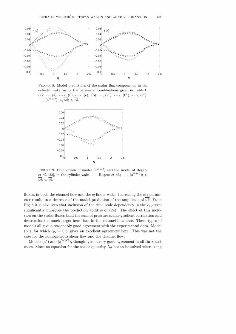
PETRA M. WIKSTROM, STEFAN WALLIN AND ARNE V. JOHANSSON 187
0 0.5 1 1.5 2 2.5−0.1
−0.08
−0.06
−0.04
−0.02
0
0.02
0.04
0.06
0 0.5 1 1.5 2 2.5−0.1
−0.08
−0.06
−0.04
−0.02
0
0.02
0.04
0.06
η η
(a) (b)
Figure 8. Model predictions of the scalar flux components, in the
cylinder wake, using the parameter combinations given in Table 1.
(a): —, (a); - - -, (b); - · -, (e). (b): —, (ar); - - -, (br); - · -, (er);
· · · , (aWWJ). ∗, uθ; , vθ.
0 0.5 1 1.5 2 2.5−0.1
−0.08
−0.06
−0.04
−0.02
0
0.02
0.04
0.06
η
Figure 9. Comparison of model (aWWJ) and the model of Rogers
et al. [22], in the cylinder wake. —, Rogers et al.; · · · , (aWWJ); ∗,uθ; , vθ.
fluxes, in both the channel flow and the cylinder wake. Increasing the cθ2 param-eter results in a decrease of the model prediction of the amplitude of uθ. FromFig. 8 it is also seen that inclusion of the time scale dependency in the cθ1-termsignificantly improves the prediction abilities of (24). The effect of this inclu-sion on the scalar fluxes (and the sum of pressure scalar-gradient correlation anddestruction) is much larger here than in the channel-flow case. These types ofmodels all give a reasonably good agreement with the experimental data. Model(br), for which cθ2 = 0.5, gives an excellent agreement here. This was not thecase for the homogeneous shear flow and the channel flow.
Models (ar) and (aWWJ), though, give a very good agreement in all three testcases. Since no equation for the scalar quantity Nθ has to be solved when using

188 A NEW EXPLICIT ALGEBRAIC MODEL FOR THE PASSIVE SCALAR FLUX
the parameter choice cθ5 = 1/2, model (aWWJ) appears particularly attractiveand can be recommended for a wide class of situations.
By using a model with the time-scale-ratio dependence of models (ar)-(aWWJ),numerical problems associated with extreme values of the time-scale ratio arealso avoided. As in the previous case, all models in Table 1 give a more realisticdescription of the scalar fluxes than a standard eddy diffusivity model, which,e.g., predicts a zero value of the uθ-component throughout the wake. The con-sequences of applying the equilibrium assumption, in the present case, may beseen in Figs. 7 and 8. Model (e) gives an excellent prediction of Πθ2 − εθ2 for|η| ≤ 1.5, whereas vθ is overpredicted in this region. This is due to the fact thatthe equilibrium assumption, Dξ1/Dt−D(ξ)
1 =0, is not quite fulfilled in this region.Since all mean scalar gradients are zero at the center line, a zero prediction of uθis obtained. To be able to give a nonzero prediction at the center line, nonlocaleffects have to be taken into account and the equilibrium assumption should notbe applied. In Fig. 6 it is seen that the transport terms are important in theregion near the center line.
In Fig. 9 a comparison of the prediction of model (aWWJ) and that of Rogerset al. [22] is made. As in the homogeneous shear flow, and in the channel flow,the model predictions are very similar for each component of the scalar flux.
5.4. Comparison with the model of Rogers et al. When comparing the(aWWJ) model with that of Rogers et al. [22] there are several things that shouldbe pointed out.
First, the model of Rogers et al. is an implicit model, which for large Reynoldsnumbers becomes a Daly & Harlow type of model and thus in this limit willunderpredict the scalar flux ratio. See Abe et al. [3] and model (c) in Table 3.This model involves an empirically determined parameter, CD, a function ofthe turbulence Reynolds number and the turbulence Peclet number, which iscalibrated against homogeneous shear flow DNS data. Model (aWWJ) is, onthe other hand, an explicit model which involves a function of the time-scaleratio, r. This function is obtained directly from the modeled equations to avoidsingularities.
Second, and perhaps the most important issue, is that the model of Rogerset al., which is formed by considering homogeneous shear flows, and neglectingthe diffusion terms in the transport equation of the dimensional scalar flux. Alsothe time evolution of the scalar flux, ∂uiθ/∂t, is assumed to be proportional tothe flux itself. This last term is then combined with the model of Πθi − εθi,and together they are modelled by Πθi − εθi − ∂uiθ/∂t = −CD(ε/2K)uiθ. Forgeneral flows exactly the same model formulation is obtained by applying theequilibrium assumption in the transport equation for the nondimensional scalarflux, (8), adding and subtracting
(∂uiθ/∂t
)/√KKθ to the right-hand side of,

PETRA M. WIKSTROM, STEFAN WALLIN AND ARNE V. JOHANSSON 189
(8), using the model Πθi−εθi−∂uiθ/∂t = −CD(ε/2K)uiθ, and finally assuming
−∂uiθ
∂t/√KKθ = −1
2ξi
(Pθ − εθKθ
+PK − ε
K
). (62)
For statistically stationary (nonhomogeneous) flows exactly the same model for-mulation is thus obtained by assuming
−12ξi
(Pθ − εθKθ
+PK − ε
K
)= 0, (63)
and using the model Πθi − εθi = −CD(ε/2K)uiθ, since ∂uiθ/∂t = 0. In thepresent non homogeneous test cases, where diffusion terms are present, i.e, thechannel flow and the cylinder wake, (63) is approximately satisfied, which maybe seen in Figs.1 and6. This explains why there are no major differences betweenthe model predictions of the model of Rogers et al., (ar), and (aWWJ), which allare based on models for Πθi − εθi that are aligned with the scalar flux, whereasmodels (ar) and (aWWJ) do not include the assumption (63). (In the case of(aWWJ) the mean scalar gradient is invoked in the model of the slow term, see(24)). Model (aWWJ) is obtained by neglecting the advection and diffusion termsin the transport equation of the nondimensional scalar flux and keeping the firstterm on the right-hand side of (8), that is, not making the assumption (63), andwould in general do a much better job in nonhomogeneous flows where (63) isnot valid (and the equilibrium assumption is appropriate).
6. Conclusions
An algebraic relation for the scalar flux in terms of mean flow quantities hasbeen formed by applying an equilibrium assumption in the transport equationfor the scalar flux. The resulting set of algebraic equations is implicit and non-linear unless the model parameter cθ5 = 1/2 is used in the model of the sum ofthe pressure scalar-gradient correlation and the destruction. A solution to thegeneral implicit relation for the normalized scalar flux in a fully explicit formis proposed. The solution is exact in two-dimensional mean flows. In three-dimensional mean flows the tensorial form is exact but an approximation for thescalar production to dissipation ratio is introduced.
The Daly–Harlow-type model, cθ2 = 1 and cθ3 = 0, can readily be transformedinto a formulation of a model for the dispersion tensor, Dij (see e.g. (22)), whichinserted into the implicit algebraic equation for ξi, yields
Dij =1 − cθ4Nθ
uiuj
k, (64)
where Nθ is given by (54). Hence, for this simplified model we have a dispersiontensor (in two-dimensional as well as in three-dimensional mean flows) that isproportional to the Reynolds stress tensor. The dependency of the mean flowgradients here enters through the scalar Nθ. For this model the distribution ofthe relative dispersion is proportional to the relative turbulence intensities in

190 A NEW EXPLICIT ALGEBRAIC MODEL FOR THE PASSIVE SCALAR FLUX
the different directions. This is analogous to the Daly & Harlow [1] model forturbulent diffusion of the Reynolds stresses. As a comparison one may note thatthe simplest eddy-diffusivity approach implicitly assumes an isotropic dispersiontensor.
From the general model formulation, it is seen that for model parametersthat deviate from cθ2 = 1 and cθ3 = 0, a dispersion tensor with principal axesdifferent from those of the Reynolds stress tensor is obtained.
With the parameter choice cθ5 = 1/2, the equation system (25) for the scalarfluxes becomes explicit without any need for solving an equation for Nθ. This isthe case for both two- and three-dimensional mean flows. The parameter choicecθ5 = 1/2 is thus very attractive. The present EASFM is then given by
ξi = −(1 − cθ4)A−1ij
(ajk +
23δjk
)Θk, (65)
where the inverse of the matrix A is given by
A−1 =
(G2 − 1
2Q1
)I−G (cSS+ cΩΩ) + (cSS+ cΩΩ)2
G3 − 12GQ1 + 1
2Q2
(66)
Predictions of the present EASFM have been compared to data for three differenttypes of flow situations. These are homogeneous shear flow, turbulent channelflow, and the flow behind a heated cylinder. With the Daly–Harlow-type model,i.e., cθ2 = 1 and cθ3 = 0, an underprediction of the uθ-component comparedto the vθ-component is obtained in all cases. Using model (aWWJ) in Table 1(given by (65) and (66) with cS = cΩ = 1 and cθ4 = 0), for which cθ5 = 1/2,very good predictions are obtained for all test cases. Since no equation for thescalar quantity Nθ has to be solved when using the parameter choice cθ5 = 1/2,model (aWWJ) is strongly recommended.
By using a model with the time-scale-ratio dependence of models (ar)-(aWWJ),numerical problems associated with extreme values of the time-scale ratio are alsoavoided. In the wake flow where the largest variations of the time-scale ratio arepresent, compared to the other two cases, the inclusion of this time-scale depen-dence is shown to be of significant importance. This time-scale ratio dependencein the cθ1-parameter is necessary to obtain good predictions in the heated cylin-der wake, using the model parameters that give good model predictions in thepresent homogeneous shear and channel-flow cases.
In a comparison of the prediction of model (aWWJ) and that of Rogers et al.[22] it is found that the model predictions are very similar for each component inall test cases of the scalar flux. Model (aWWJ), which is obtained by neglectingthe advection and diffusion terms in the transport equation of the nondimen-sional scalar flux and keeping the first term on the right-hand side of (8), thatis, not making the assumption (63), would in general do a much better job innonhomogeneous flows where (the equilibrium assumption is appropriate and)(63) not is valid.

References 191
An explicit algebraic scalar flux model as proposed here ((65) and (66)) shouldsuitably be used together with an appropriate EARSM for the Reynolds stresses.To make the model complete model equations for θ2 and εθ are needed to beable to determine the time-scale ratio r.
References
[1] Daly, B. J. & Harlow, F. H. 1970 Transport equations in turbulence. Phys.Fluids 13, 2634–2649.
[2] Kim, J., & Moin, P. 1989 Transport of passive scalars in a turbulent channelflow. in proc. Turbulent Shear Flows 6, Toulouse Sept. 7-9 1987, Springer,85–96
[3] Abe, K., & Suga, K. 1998 Large eddy simulation of passive scalar fieldsunder several strain conditions. in proc. Turbulent Heat Transfer II, Manch-ester May 31 – June 5, 2, 8-15–8-30.
[4] Adumitroaie, V., Taulbee, D. B. & Givi, P. 1997 Explicit Algebraic Scalar-Flux Models for Turbulent Reacting Flows. A. i. ch. e. J. 43, 1935–2147.
[5] Girimaji, S. S. & Balachandar, S. 1998 Analysis and modeling of boyancy-generated turbulence using numerical data. Int. J. Heat Mass Transfer 41,915–929.
[6] Abe, K., Kondoh, T. & Nagano, Y. 1996 A two-equation heat transfer modelreflecting second-moment closures for wall and free turbulent flows. Int. J.Heat and Fluid Flow 17, 228–237.
[7] Shih, T. H. & Lumley, J. L. 1993 Remarks on Turbulent Constitutive Re-lations. Mathl. Comput. Modelling 18(2), 9–16.
[8] Shih, T. H. 1996 Constitutive relations and realizability of single-point tur-bulence closures. Turbulence and Transition Modelling, M. Hallback, D.S.Henningson, A.V. Johansson & P.H. Alfredsson (eds), Vol 2, Kluwer.
[9] Shabany, Y. & Durbin, P. A. 1997 Explicit Algebraic Scalar Flux Approxi-mation. AIAA J. 35, 985–989.
[10] Johansson, A. V. & Wallin, S. 1996 A new explicit algebraic Reynolds stressmodel. Proc. Sixth European Turbulence Conference, Lausanne, July 1996,Ed. P. Monkewitz, 31–34.
[11] Girimaji, S. S. 1995 Fully explicit and self-consistent algebraic Reynoldsstress model. Theor. Comp. Fluid Dyn. 8, 387.
[12] Wallin, S. & Johansson, A. V. 1996 A complete explicit algebraic Reynoldsstress turbulence model including an improved near-wall treatment. Proc.Flow Modeling and Turbulence Measurements VI, Tallahassee FL, C.-J.Chen, C. Shih, J. Lienau & R.J. Kung (eds), 399–406, Balkema, Rotterdam.
[13] Wallin, S. & Johansson, A. V. 2000. An explicit algebraic Reynolds stressmodel for incompressible and compressible turbulent flows. To appear in J.Fluid Mech. 403, 89–132.

192 References
[14] Rodi, W. 1972 The prediction of free turbulent boundary layers by use ofa two equation model of turbulence. Ph.D. thesis, University of London.
[15] Rodi, W. 1976 A new algebraic relation for calculating the Reynoldsstresses. Z. angew. Math. Mech. 56, T219–221.
[16] Launder, B. E. 1978 Heat and mass transport. In Turbulence, P. Bradshaw(ed.), Springer, Berlin, 231–287.
[17] Craft, T. J., Launder, B. E. 1996 Recent developments in second-momentclosure for boyancy-affected flows. Dynamics of Atmospheres and Oceans23, 99–114.
[18] Rogers, M.M., Moin, P. & Reynolds, W.C. 1986 The structure and modelingof the hydrodynamic and passive scalar fields in homogeneous turbulentshear flow. Dept. Mech. Engng. Rep. TF-25, Stanford University, Stanford,California.
[19] Wikstrom, P. M. and Johansson, A. V. 1998 DNS and scalar-flux transportmodelling in a turbulent channel flow. in proc. Turbulent Heat Transfer II,May 31-June 5, Manchester, 1998.
[20] Wikstrom, P. M., Hallback, M., and Johansson, A. V. 1998 Measurementsand heat-flux transport modelling in a heated cylinder wake. Intl. J. HeatFluid Flow 19, 556–562.
[21] Browne, L. W. B., & Antonia, R. A. 1986 Reynolds shear stress and heatflux measurements in a cylinder wake. Phys. Fluids A. 29, 709–713.
[22] Rogers, M.M., Mansour, P. & Reynolds, W.C. 1989 An algebraic model forthe turbulent flux of a passive scalar. J. Fluid Mech. 203, 77–101.

Paper 6
6


195
AN EFFICIENT EXPLICIT ALGEBRAIC REYNOLDS STRESS k-ωMODEL (EARSM) FOR AERONAUTICAL APPLICATIONS
Stefan WallinThe Aeronautical Research Institute of Sweden (FFA), Bromma, Sweden
Abstract. The self-consistent explicit algebraic Reynolds stress model (EARSM)proposed by Wallin & Johansson (1997) with the k-ω wo-equation transportmodel as platform was the starting point for some further developments. The orig-inal near-wall damping function was reformulated in terms of andan additional alternative without any damping functions whatsoever was intro-duced. The EARSM approach clearly improves the shock position for transonicwings without significal increase in computational cost. The EARSM may beexpressed as an extension to an eddy-viscosity model and thus no major problemsshould be expected in implementing EARSM into a flow solver with existing two-equation eddy-viscosity models.
1. Introduction
Standard two-equation models based on the eddy-viscosity assumption are still domi-nating in the context of industrial flow computations. In flows with strong effects ofstreamline curvature, adverse pressure gradients, flow separation or system rotation,such models fail to give accurate predictions. Turbulence models based on the transportequations for the individual Reynolds stresses have the natural potential for dealingwith, e.g., the associated complex dynamics of intercomponent transfer. The eddy-vis-cosity hypothesis may in this context be said to be replaced by transport equations forthe individual Reynolds stress anisotropies. As yet, there are non-trivial numericalaspects of flow computations with such models in complex flow situations. This repre-sents an active area of research. In parallel with such efforts there has been a considera-ble renewed interest in various forms of explicit algebraic approximations of theanisotropy transport equations, see e.g. Pope (1975), Gatski & Speziale (1993), Gir-imaji (1995), Johansson & Wallin (1996) and Wallin & Johansson (1997).
The model proposed by Wallin & Johansson has been proven to give importantimprovements over standard two-equation models based on the eddy-viscosity assump-tion in flows with strong effects of streamline curvature, adverse pressure gradients,flow separation or system rotation. The near-wall formulation in the model is, however,based on which may cause problems in some situations.
In the present work the near-wall formulation in the model proposed by Wallin &Johansson will be revised in terms of the wall distance which replaces the -depend-ency. Moreover, a simplified version is proposed without near-wall damping functionswhatsoever which may be attractive for computation of complicated 3D flows.
Rey ky ν⁄≡
y+
y+

196 AN EFFICIENT k-ω EARSM FOR AERONAUTICAL APPLICATIONS
2. Description of the models
The turbulence models that will be described here are variations of the explicit alge-braic Reynolds stress model (EARSM) described in detail by Wallin & Johansson(1997). That model is based on a recalibrated Launder, Reece & Rodi (1975) modelwhich is a differential Reynolds stress model. A self-consistent and fully explicit alge-braic relation for the Reynolds stresses in terms of the mean flow field is then obtainedby applying the so-called ‘equilibrium assumption’, Rodi (1972 & 1976), where theadvection and diffusion of the Reynolds stress anisotropy is neglected.
The model is based on transport equations for the turbulent kinetic energy and thespecific dissipation rate and we are recommending two options: (i) EARSM basedon the Wilcox (1988) standard model denoted ‘WJ_skw’ and (ii) EARSM basedon the Wilcox (1994) low-Reynolds number model denoted ‘WJ_kw’. There isactually a third option that is an eddy-viscosity model obtained from further simplifica-tion of (i). That is (iii) Linear EARSM based on the Wilcox (1988) standardmodel denoted ‘LWJ_kw’.
A well known problem with these options is that the model is unphysicallysensitive to the free-stream turbulence level. That has recently been resolved by Kok(1999) by adding a cross-diffusion term in the -equation. An interesting, but not thor-oughly tested alternative is thus EARSM based on Kok , alternative (iv).
Which of these options that should be recommended depends on the application. Thefollowing may be used as a guide:
(i) EARSM based on standard is more simple to implement and needs nowall-distance information. The turbulent kinetic energy and the Reynolds stress profilesare qualitatively wrong in the near-wall region, , but the velocity profiles andskin friction are correct. This alternative is thus most suitable as an engineering tool forcomplicated 3D flows where detailed information of the near-wall turbulence is notneeded.
(ii) EARSM based on low-Reynolds number is somewhat more complex andneeds the distance to the closest wall. The model is, however, independent of the localwall skin friction or . The influence by the near-wall damping functions are limitedto the very near-wall region and are practically zero for . For this reason, itshould not be an important issue how multiple walls and corners are treated. The turbu-lent kinetic energy and the Reynolds stress profiles are well predicted also in the near-wall region. This alternative should thus be used if detailed information of the near-wallturbulence is needed.
(iii) Linear EARSM based on standard model is only motivated from thesomewhat simplified implementation. The model is actually an eddy-viscosity modeland thus only the routine that computes the eddy viscosity needs to be modified. Someof the prediction capabilities of the full EARSM, (i) or (ii), is lost but this alternative isstill better than the more ad-hoc standard eddy-viscosity models with constant .
kω
k ω–k ω–
k ω–
k ω–
ωk ω–
k ω–
y+ 100<
k ω–
y+
y+ 100>
k ω–
Cµ

S. WALLIN 197
(iv) EARSM based on Kok is similar to alternative (i) regarding implementa-tion and prediction capabilities since the only difference is a cross-diffusion term addedto the -equation. The advantage with this alternative is that the unphysical free-stream dependency in the standard is eliminated. However, this model is notthoroughly tested yet.
These three models will be described with special emphasis on the extension to anEARSM.
2.1. EARSM based on standard k-ω
2.1.1. Transport equations. The transport equations for and read
(1)
where
. (2)
The production of the turbulent kinetic energy is defined as
(3)
and the dissipation rate
. (4)
, , , and are the model con-stants.
In the original eddy-viscosity model the Reynolds stresses are obtained from
where (5)
and the turbulent viscosity is given by
. (6)
2.1.2. Reynolds stresses. The Reynolds stresses expressed by EARSM may bewritten in terms of an effective turbulent viscosity and an extra anisotropy
. (7)
k ω–
ωk ω–
k ω
DDt------ ρk( ) P ρε–
x j∂∂ µ
µT
σk------+
x j∂
∂k+=
DDt------ ρω( ) αω
k----P βρω2–
x j∂∂ µ
µT
σω-------+
x j∂
∂ω+=
DDt------
t∂∂
U j x j∂∂
+≡
P ρuiu j x j∂∂Ui–≡
ε β*ωk≡α 5 9⁄= β 3 40⁄= β* 9 100⁄= σk 2.0= σω 2.0=
ρuiu j23---ρkδij 2µT Sij
*–= S*ij
12---
x j∂∂Ui
xi∂∂U j 2
3---
xk∂∂Ukδij–+
=
µTρkω------=
ρuiu jµT aij
(ex)
ρuiu j23---ρkδij 2µT Sij
*– ρkaij(ex)
+=

198 AN EFFICIENT k-ω EARSM FOR AERONAUTICAL APPLICATIONS
The effective turbulent viscosity then reads
(8)
and the extra anisotropy
. (9)
The invariants are
, and . (10)
Here , and denotes second rank tensors. denotes the trace and (or) is the identity matrix. The inner product of two matrices is defined as
. The normalized mead strain- and rotation rate tensors aredefined as
and (11)
where is the turbulent time-scale. The dimensional strain- and rotation rate tensorsare
and . (12)
In the near-wall region, viscous effects become important and the turbulent time-scale in (11) need to be limited by the Kolmogoroff time scale as proposed by Durbin(1993)
(13)
where is a model constant.The -coefficients in (8) and (9) are given by
(14)
with the non-singular denominator
. (15)
is given by
µT12--- β1 IIΩβ6+( )ρkτ–=
a(ex) β3 Ω2 1
3---IIΩ I–
β4 SΩ ΩS–( )+=
β6 SΩ2 Ω2S IIΩS–23---IV I–+
β9 ΩSΩ2 Ω2SΩ–( )+ +
IIS tr S2 = IIΩ tr Ω2 = IV tr SΩ2 =
a S Ω tr IδijSS( )ij S2( )ij SikSkj≡ ≡
Sij τS*ij= Ωij τΩ*
ij=
τ
S*ij
12---
x j∂∂Ui
xi∂∂U j 2
3---
xk∂∂Ukδij–+
= Ω*ij
12---
x j∂∂Ui
xi∂∂U j–
=
τ maxkε-- Cτ
µρε------,
=
Cτ 6.0=β
β1
N 2N2 7IIΩ–( )Q
------------------------------------–= β312N 1– IV
Q----------------------–=
β4
2 N2 2IIΩ–( )Q
-------------------------------–= β66NQ
-------–= β96Q----=
Q56--- N2 2IIΩ–( ) 2N2 IIΩ–( )=
N

S. WALLIN 199
(16)
where
, (17)
and
. (18)
When computing the third root one need to make sure that the real root is returned evenfor negative arguments and the arccos function should return an angle between and
. is a model constant.In 2D mean flows the -coefficients are
(19)
and the relation (9) simplifies significantly.
2.2. EARSM based on low-Re k-ω. The transport equation for and are givenby (1) to (3) and the dissipation rate is given by (4) as for the standard model.The differences enter through the model coefficients that in the case of low-Reynoldsnumber are functions of the turbulent Reynolds number .
These functions read:
(20)
where the turbulent Reynolds number is defined as
. (21)
, , , , and are the model constants.
N
C1'
3------- P1 P2+( )1 3/ P1 P2–( )1 3/+ + P2 0≥,
C1'
3------- 2 P1
2 P2–( )1 6/ 13---arccos
P1
P12 P2–
-----------------------
cos+ P2 0<,
=
P1
C1'2
27----------
920------IIS
23---IIΩ–+
C1'= P2 P12
C1'2
9----------
910------IIS
23---IIΩ+ +
3
–=
C1'94--- c1 1–( )=
0π c1 1.8=
β
β165---–
N
N2 2IIΩ–-----------------------= β4
65---–
1N2 2IIΩ–-----------------------=
β3 0= β6 0= β9 0=
k ωε k ω–
k ω– ReT
β* 9100---------
5 18⁄ ReT Rβ⁄( )4+
1 ReT Rβ⁄( )4+-----------------------------------------------=
α 59---α0 ReT Rω⁄+
1 ReT Rω⁄+---------------------------------- α*( ) 1–⋅=
α*β 3⁄ ReT Rk⁄+
1 ReT Rk⁄+------------------------------------=
ReTρkωµ-------=
Rβ 8= Rω 2.7= Rk 6= α0 1 10⁄= β 3 40⁄=

200 AN EFFICIENT k-ω EARSM FOR AERONAUTICAL APPLICATIONS
2.2.1. Reynolds stresses. The Reynolds stresses is also here written in terms ofthe effective turbulent viscosity and the extra anisotropy as in (7) but here anear-wall damping function needs to be introduced. The effective turbulent viscositythen reads
(22)
and the extra anisotropy
(23)
where
(24)
and is an additional model constant.The near-wall damping function in (22) and (23) was original defined in terms ofby Wallin & Johansson (1997) but has later been redefined in terms of . The
near-wall damping is needed when EARSM is used together with low-Reynoldsnumber two-equation models with correct near-wall asymptotic behaviour.
(25)
where
. (26)
and are model constants. The -coefficients in (22)and (23) are defined as previous in (14) to (17) or in (19) for 2D mean flows.
2.3. Linear EARSM based on standard k-ω. An alternative to EARSM based onstandard that is even more simple to implement, since it actually is an eddy-vis-cosity model, is here described. The approach is to keep only the eddy-viscosity part ofthe relation (7) which means that . Some of the physics covered of the fullEARSM is naturally missing in this approach and it cannot be motivated fromincreased robustness or decreased computational cost. However, as an eddy-viscositymodel this approach is based on a more sound basis compared to standard eddy-viscos-
ρuiu jµT aij
(ex)
µT12--- f 1 β1 IIΩβ6+( )ρkτ–=
a(ex)
1 f 12–( )
3B2 4–
max IIS IISeq,( )
------------------------------- S2 13---IIS I–
=
f 12β3 Ω2 1
3---IIΩ I–
f 12β4 1 f 1–( )
B2
2max IIS IISeq,( )
----------------------------------–
SΩ ΩS–( )+ +
f 1β6 SΩ2 Ω2S IIΩS–23---IV I–+
f 12β9 ΩSΩ2 Ω2SΩ–( )+ +
IISeq 405c1
2
216c1 160–-----------------------------=
B2 1.8=f 1
y+ Rey
f 1 1 exp CyA Rey– CyBRey2–( )–=
Reyρ kyµ
-------------≡
CyA 0.092= CyB 1.2 10 4–⋅= β
k ω–
aij(ex)
0=

S. WALLIN 201
ity models with constant . The only motivation for this approach is that only theroutine that computes the eddy-viscosity needs to be modified.
2.4. EARSM based on Kok k-ω. The dependenc on free-stream -values in themodel has been resolved by Kok (1999) by adding a cross-diffusion term in the
-equation and modifying the diffusion coefficients.This model is identical to EARSM based on standard (see section 2.1) except
a few details. The transport equation for reads
(27)
where the diffusion coefficients are and . The diffusion coefficientin the -equation (1) is modified to .
3. Implementation
3.1. Formulation in terms of an effective viscosity. The Reynolds stressesexpressed by EARSM is written in terms of an effective turbulent viscosity and anextra anisotropy . The reason for this is that many CFD solvers already have dif-ferent eddy-viscosity two-equation models implemented and that many routines may bereused when the model is formulated in terms of an effective turbulent viscosity .Our experience is that it is sufficient only to consider the effective turbulent viscosity
when determining the stability limit for explicit methods or the system Jacobian forimplicit methods. The extra terms associated with the extra anisotropy may betreated as a fully decoupled source term without loss of performance of the solutionmethod.
3.2. Terms to be modified. 3.2.1. Production of the turbulent kinetic energy. Theproduction of the turbulent kinetic energy is defined as
(28)
and needs no further modelling since the Reynolds stresses are explicitly known. In aneddy-viscosity two-equation model, this term is modelled as
. (29)
Many important physical aspects are lost through this assumption, like effects ofstreamline curvature and local and global rotation and this term is thus the most impor-tant to modify. By using the effective turbulent viscosity in (29) and by adding the
Cµ
ωk ω–ω
k ω–ω
DDt------ ρω( ) αω
k----P βρω2–
x j∂∂ µ
µT
σω-------+
x j∂
∂ω σdρω----max
x j∂∂k
x j∂∂ω
0, + +=
σω 2.0= σd 0.5=k σk 1.5=
µTaij
(ex)
µT
µTaij
(ex)
P ρuiu j x j∂∂Ui–≡
P(EVM)2µT Sij
* 23---ρkδij–
x j∂
∂Ui=
µT

202 AN EFFICIENT k-ω EARSM FOR AERONAUTICAL APPLICATIONS
contribution from the extra anisotropy the original definition of the production of theturbulent kinetic energy is preserved
. (30)
3.2.2. The turbulent transport of momentum. The second most important term to mod-ify is the turbulent transport of momentum in the momentum equation. This term is alsoexactly defined in terms of the Reynolds stresses and reads
. (31)
In an eddy-viscosity two-equation model, this term is modelled as
. (32)
Also for this term many important physical aspects are lost through this assumption,like turbulence induced secondary motions. By using the effective turbulent viscosity
in (29) and by adding the contribution from the extra anisotropy the original defini-tion of turbulent transport of momentum is preserved
. (33)
3.2.3. Turbulent transport terms. There are also a number of other turbulent transportterms, but these terms needs to be modelled even in terms of the Reynolds stresses. Ineddy-viscosity two-equation models, these terms are most commonly modelled usinggradient diffusion where the diffusion coefficients are related to the turbulent viscosity.Also here the effective turbulent viscosity should be used, but no further modificationsof these terms are necessary.
It is, however, possible to adopt some more elaborate modelling in terms of the Rey-nolds stresses also for these terms, but in that case one must use the near-wall correctEARSM including near wall damping functions.
3.3. Wall boundary conditions. The physical wall boundary conditions on and are
, and (34)
where is the wall distance in the wall-normal direction. In a cell centred FVM, theboundary condition should result in a correct wall flux. That is obtained by setting
P P(EVM) ρkaij(ex)
x j∂∂Ui–=
T i x j∂∂ ρuiu j–( )≡
T i(EVM)
x j∂∂ 2µT Sij
* 23---ρkδij–
=
µT
T i T i(EVM)
x j∂∂ ρkaij
(ex)( )–=
kω
k 0=y∂
∂k 0= ω 6µβρy2------------→
y

S. WALLIN 203
for the convective fluxes and for the viscous fluxes. Index indi-cates the dummy cell value while index indicates the first interior cell.
The boundary condition on is where the wall value is givenby
(35)
where is the wall normal distance to the first cell centre (for a cell centredscheme) and is a constant. Menter (1994) originally chosen that constant tobut later Hellsten (1998) suggested a value of which minimizes the influence of thenear-wall grid spacing. The approach of Hellsten was adopted here, thus .
3.4. General numerical discretization. The numerical treatment of standard two-equation turbulence models described by Eliasson (1999), concerning e.g. multigrid,positiveness, second order upwind scheme, was adopted also for the EARSM approach.
4. Shock - turbulence interaction
A shock may cause problems in computations using standard eddy-viscosity two-equa-tion models. The problem is that the turbulence may grow at the shock and the growthincreases typically with increasing grid density. This problem do not occur in theboundary layer and if EARSM is used. This phenomena is here analysed.
Let us consider a model problem, a one-dimensional moving shock. The shockvelocity is , the velocity jump over the shock and the shock thickness . Thethickness of the shock is in high Reynolds number flows a function of the numericalresolution of the shock.
Following the shock, the equation for the turbulent kinetic energy becomes, if thediffusion and dissipation are neglected
(36)
and by integrating once
. (37)
We have here assumed that the production may be considered as constant over theshock.
The production is
(38)
since the anisotropy is limited to around unity. The integrated -equation thenbecomes
k0 k– 1= k0 k1= 0
1ω ω0 2ωwall ω1–=
ωwall Cω-w6µ
βρy1 2⁄2
------------------=
y1 2⁄
Cω-w 101.5
Cω-w 1.5=
V ∆V ∆x
Vx∂∂ ρK( ) P=
∆ ρK( ) PV---- xd∫ P∆x
V------≈=
P ρuiu j x j∂∂Ui– ρK aij
23---δij+
x j∂
∂Ui– ρK a1123---+
x∂
∂U– ρK
∆V∆x--------∼= = =
K

204 AN EFFICIENT k-ω EARSM FOR AERONAUTICAL APPLICATIONS
. (39)
The turbulence growth over the shock is thus independent of the shock thickness, i.e.the resolution of the shock.
In an eddy-viscosity model the production is modelled as
(40)
and the integrated -equation becomes
(41)
and the turbulence growth over the shock increases with decreasing shock thickness.For high Reynolds numbers, the turbulence may grow almost unbounded and thus gen-erates unphysical high turbulence levels downstream of the shock. In fact also in sub-sonic flows, any small disturbance in the velocity field or grid may generate unphysicalgrowth of free stream turbulence.
To avoid that effect in eddy-viscosity models the production may be limited. Oneoften used form is to limit the production by the dissipation rate where issome sufficiently high number. The problem with this form is that in rapidly growingturbulence the production rate is, and should be, independent of the dissipation rate. Amore appropriate form is obtained by considering the relation (38)
(42)
which could serve as an upper limit for . This limit is related to the realizability con-straint that the norm of the anisotropy should be limited. The limit could also beexpressed in terms of the eddy-viscosity production as
(43)
and the limited production is obtained by which is easilyimplemented. for which implies that the limitwould not be active for . The limitor should thus not interfere with the predic-tion capability of the model.
This problem does not occur for the proposed EARSM since the production is herenot modelled using the eddy-viscosity hypothesis. Even the linear EARSM describedprevious does not have this deficiency. The reason for this is that the effective turbulentviscosity, or the effective , is a function of the strain rate such that
for large strain rates.
∆ ρK( ) ρK∆VV
--------∼
P(EVM)2µT Sij
* 23---ρKδij–
x j∂
∂Ui= µT∆V∆x-------- 2
∼
K
∆ ρK( ) µT∆V( )2V∆x
---------------∼
P Cρε< C
P ρK aij23---δij+
x j∂
∂Ui– ρK aij Sij* ρK Sij
*<≤ ρK Sij* S ji
*= =
P
P(lim) ρKP(EVM)
µT-----------------=
P min P(EVM) P(lim),( )=P(EVM) P(lim)< P(EVM) ε Cµ f µ( )⁄<
P ε⁄ 10<
CµCµ 1 Sij
* S ji*⁄→

S. WALLIN 205
5. Test cases
5.1. RAE2822: 2D transonic wing profile. The two-dimensional transonic wingprofile RAE2822, case10 illustrates the behaviour of the proposed model. The wing ishighly loaded and a boundary layer separation occurs at the shock impingement. Figure1 shows the wall pressure and skin friction coefficients, and . Standard eddy-viscosity models, like the Wilcox (1988) standard model denoted ‘std_kw’, pre-dict a shock position downstream of the observed one. The proposed EARSM approachclearly improves the shock position and the results are very much in line with differen-tial Reynolds stress computations by Hellström et al. (1994). For this case there are nomajor difference in computational results between EARSM based on standard or low-Reynolds number , ‘WJ_skw’ or ‘WJ_kw’. The eddy-viscosity version‘LWJ_kw’ gives, however, a shock position downstream of the EARSM’s. Also thecomputational results using the Menter (1994) SST model, ‘SST_kw’, is shown in thefigure. That model gives a somewhat better shock position. The best prediction of theshock position is, however, obtained with EARSM based on the Kok model. Fig-ure 3 shows the velocity profiles at different -positions.
There are still some deviations from the experimental data and there are other com-putations published on this case that have better agreements. The reason for this is thatthere exists a number of different geometries for this case, the measured or designgeometry with or without an additional camber correction. For this case the measuredgeometry with the camber correction was used.
The -residual convergence history is shown in figure 2. The eddy-viscositymodel has the best convergence rate but the different EARSM’s have similar
convergence rates. The EARSM approach increases the computational time with lessthat 10% and the different computations were obtained by using the same numericalsettings (CFL, multigrid levels, upwind discretization, et.c.). In flows without separa-tion the convergence curves are even closer to each other.
5.2. LANN: 3D transonic wing. A further example for illustrating the model inthree-dimensional flows is the transonic LANN-wing, measured by Horsten et al.(1983). Figure 4 shows the pressure coefficient distribution at different spanwise posi-tions and figure 5 shows the surface pressure distribution as well as the computed skinfriction lines. Also here the EARSM approach (‘WJ_skw’) improves the predictedshock position compared to the Wilcox (1988) standard model (‘std_kw’).
C p C fk ω–
k ω–
k ω–x
RMS ρ( )k ω–
k ω–

206 AN EFFICIENT k-ω EARSM FOR AERONAUTICAL APPLICATIONS
FIGURE 1: Predicted and distributions compared to measurements forthe RAE2822 wing profile at , and(Case 10). The standard eddy-viscosity model (std_kw) and MenterSST (SST_kw) compared to the EARSM based on standard(WJ_skw), EARSM based on low-Reynolds number (WJ_kw),EARSM based on Kok (WJ_Kkw marked with small squares) and theLinear EARSM based on standard (LWJ_kw). Experimental data fromCook et al. (1979).
x/c
Cp
0.00 0.20 0.40 0.60 0.80 1.00 1.00
0.50
0.00
-0.50
-1.00
-1.50 std_kwSST_kwWJ_skwWJ_kwLWJ_skwWJ_Kkwexpr
x/c
Cf
0.00 0.20 0.40 0.60 0.80 1.00 -0.0060
-0.0020
0.0020
0.0060
0.0100 std_kwSST_kwWJ_skwWJ_kwLWJ_skwWJ_Kkwexprzero
C p C fMa 0.754= α 2.57= Re 6.2 10
6⋅=k ω–
k ω– k ω–k ω–
k ω–k ω–

S. WALLIN 207
FIGURE 2: -residual convergence history for the RAE2822 wing profile. Thestandard eddy-viscosity model (std_kw) compared to the EARSMbased on standard (WJ_skw), EARSM based on low-Reynolds number
(WJ_kw) and the Linear EARSM based on standard (LWJ_kw).
iter
rho_rms
0. 2000. 4000. 6000. -6.0
-4.0
-2.0
0.0 std_kwWJ_skwWJ_kwLWJ_skw
ρk ω–
k ω–k ω– k ω–

208 AN EFFICIENT k-ω EARSM FOR AERONAUTICAL APPLICATIONS
FIGURE 3: Predicted velocity profiles at different -positions compared tomeasurements for the RAE2822 wing profile at , and
(Case 10). The standard eddy-viscosity model(std_kw) and Menter SST (SST_kw) compared to the EARSM basedon standard (WJ_skw), EARSM based on low-Reynolds number(WJ_kw), EARSM based on Kok (WJ_Kkw marked with small squa-res) and the Linear EARSM based on standard (LWJ_kw). Experimen-tal data from Cook et al. (1979).
U/Uf
y/c
0.0 0.4 0.8 1.2 0.00
0.01
0.02
0.03
x/c=0.404
U/Uf
y/c
-0.2 0.2 0.6 1.0 0.00
0.01
0.02
0.03 std_kwSST_kwWJ_skwWJ_kwLWJ_skwWJ_Kkwexpr
x/c=0.650
U/Uf
y/c
0.0 0.4 0.8 1.2 0.00
0.01
0.02
0.03
x/c=0.750
U/Uf
y/c
0.0 0.4 0.8 1.2 0.000
0.015
0.030
0.045 std_kwSST_kwWJ_skwWJ_kwLWJ_skwWJ_Kkwexpr
x/c=0.900
U/Uf
y/c
0.0 0.4 0.8 1.2 -0.04
0.00
0.04
0.08
x/c=1.000
U/Uf
y/c
0.0 0.4 0.8 1.2 -0.04
0.00
0.04
0.08 std_kwSST_kwWJ_skwWJ_kwLWJ_skwWJ_Kkwexpr
x/c=1.025
xMa 0.754= α 2.57=
Re 6.2 106⋅= k ω–
k ω–k ω– k ω–
k ω–k ω–

S. WALLIN 209
FIGURE 4: Predicted distribution at different spanwise positions comparedto measurements for the LANN wing at , and
. The standard eddy-viscosity model ( ) compa-red to the EARSM based on standard ( ). Experimental data fromHorsten et al. (1983).
0.200 0.325
0.475 0.650
0.825 0.950
C pMach 0.82= α 2.60=
Re 7.16 106⋅= k ω–
k ω–

210 AN EFFICIENT k-ω EARSM FOR AERONAUTICAL APPLICATIONS
FIGURE 5: Predicted skin friction lines for the LANN wing at ,and . The standard eddy-viscosity model
(top) compared to the EARSM based on standard (bottom).
6. Concluding remarks
The EARSM approach was shown to improve the shock position over standard eddy-viscosity two-equation models, for highly loaded transonic wings, without significalincreased computational cost. The EARSM without damping functions with the stand-ard model as the platform is recommended for this kind of problems. The addi-tional accuracy in the near-wall region, that the EARSM with damping functionsprovides, is probably not needed in the cases studied here.
The Kok model is an interesting alternative since the erroneously free-streamdependency in standard models have been removed. The EARSM based on that
k ω–
EARSM
Mach 0.82=α 2.60= Re 7.16 10
6⋅= k ω–k ω–
k ω–
k ω–k ω–

S. WALLIN 211
model also shows the best predictions for the RAE2822 case. This combination(EARSM + Kok ) should, thus, be further investigated and tested, especially con-cerning the free-stream dependency.
The Menter SST model predicts the shock position well for the RAE2822 and couldalso be recommended for these kind of flow problems. This model is, however, aneddy-viscosity model with an empirical limitation on the turbulent viscosity and thuslacks the generality of the more fundamental EARSM. That is obvious in rotationaldominated flows where the EARSM has the correct qualitative behaviour while eddy-viscosity models and in some cases also incomplete quadratic EARSMs fail, reportedby Wallin & Johansson (1997).
Acknowledgment
This work has been carried out within the the AVTAC Project (Advanced ViscousFlow Simulation Tools for Complete Civil Transport Aircraft). AVTAC is a collabora-tion between British Aerospace, DASA, CASA, Dassault Aviation, SAAB, Alenia,DLR, ONERA, CIRA, FFA and NLR. The project is managed by British Aerospaceand is funded by the CEC under the IMT initiative (Project Ref: BRPR CT97-0555)
References
[1] Cook, P.H., MacDonald, M.A. & Firmin, M.C.P. 1979 Aerofoil 2822 - Pressure dis-tributions, boundary layer and wake measurements. AGARD AR 138.
[2] Durbin, P.A. 1993 Application of a near-wall turbulence model to boundary layersand heat transfer. Int. J. Heat and Fluid Flow 14, 316–323.
[3] Eliasson, P. 1999 A robust and positive scheme for viscous, compressible steadystate solutions with two-equation turbulence models. FFA TN 1999-81.
[4] Gatski, T.B. & Speziale, C.G. 1993 On explicit algebraic stress models for complexturbulent flows. J. Fluid Mech. 254, 59–78.
[5] Girimaji, S.S. 1995 Fully-explicit and self-consistent algebraic Reynolds stressmodel. ICASE Report No. 95-82.
[6] Hellsten, A. 1998 On the solid-wall boundary condition of in the -type tur-bulence models. Helsinki University of Technology, Report No B-50, Series B.
[7] Hellström, T., Davidson, L. & Rizzi A. 1994 Reynolds stress transport modelling oftransonic flow around the RAE2822 airfoil. AIAA 94-0309. 32nd Aerospace SciencesMeeting, Reno, Jan. 1994.
[8] Horsten, J.J., Den Boer, R.G. & Zwaan, R.J. 1983 Unsteady transonic pressuremeasurements on a semi-span wind tunnel model of a transport-type supercriticalwing (LANN model). AFWAL-TR-83-3039.
[9] Johansson, A.V. & Wallin, S. 1996 A new explicit algebraic Reynolds stress model.Proc. Sixth European Turbulence Conference, Lausanne, P. Monkewitz (ed). 31–34.
[10] Kok, J.C. 1999 Resolving the dependence on free-stream values for the tur-bulence model. Submitted to AIAA J.
k ω–
ω k ω–
k ω–

212 AN EFFICIENT k-ω EARSM FOR AERONAUTICAL APPLICATIONS
[11] Launder, B.E. Reece, G.J. & Rodi, W. 1975 Progress in the development of a Rey-nolds-stress turbulence closure. J. Fluid Mech. 41, 537–566.
[12] Menter, F.R. 1994 Two-equation eddy-viscosity turbulence models for engineeringapplications. AIAA J. 32, 1598–1604.
[13] Pope, S.B. 1975, A more general effective-viscosity hypothesis. J. Fluid Mech. 72
331–340.[14] Rodi, W. 1972 The prediction of free turbulent boundary layers by use of a twoequation model of turbulence. Ph.D. thesis, University of London.
[15] Rodi, W. 1976 A new algebraic relation for calculating the Reynolds stresses. Z.angew. Math. Mech. 56, T219–221.
[16] Wallin, S & Johansson, A. V. 1996, A new explicit algebraic Reynolds stress tur-bulence model including an improved near-wall treatment. Proc. Flow Modeling andTurbulence Measurements VI, Tallahassee, Chen, Shih, Lienau & Kung (eds).
[17] Wallin, S. & Johansson, A.V. 1997 A complete explicit algebraic Reynolds stressmodel for incompressible and compressible turbulent flows. FFA TN 1997-51 (submit-ted for publication). Also to appear in J. Fluid Mech, 403, 89-132, (2000).
[18] Wilcox, D.C. 1988 Reassessment of the scale-determining equation for advancedturbulence models. AIAA J. 26, 1299–1310.
[19] Wilcox, D.C. 1994 Simulation of transition with a two-equation turbulence model.AIAA J. 32, 247–255.

Paper 7
7


215
A ROBUST AND POSITIVE SCHEME FOR VISCOUS, COMPRES-SIBLE STEADY STATE SOLUTIONS WITH TWO-EQUATION TURBU-
LENCE MODELS
Peter Eliasson and Stefan WallinThe Aeronautical Research Institute of Sweden (FFA), Bromma, Sweden
Abstract. An efficient and robust method has been designed for the simulation ofthe compressible Navier-Stokes equations with two-equations turbulence models.The compressible Navier-Stokes equations are integrated explicitly to steady stateand a novel approach is used to maintain the positivity of the turbulent quantities.The novel approach is based on a conservative estimate of the characteristics ofthe turbulent equations leading to a restriction of the local time step determinedby the residual. As steady state is approached the residual and the restriction ofthe time step is reduced and hence the asymptotic rate of convergence is notaffected. Multigrid is used to accelerate the convergence and a similar approach isused when adding the corrections to guarantee a positive scheme. A higher orderrestriction operator improves the robustness and the performance of the scheme. Itis demonstrated that the higher order restriction can improve the rate of conver-gence, especially for ‘bad’ grids with large stretchings and locally large variationsin grid size. Numerical results are presented for a model problem and on aRAE2822 airfoil.
1. Introduction
The design of efficient and robust numerical algorithms is essential for the simulationof compressible turbulent flows, especially for engineering-type applications. The mainobjective of this paper is to demonstrate new approaches to gain increased robustness inthe iteration of an explicit Navier-Stokes solver coupled with a two-equation turbulencemodel and accelerated with a multigrid method.
It is well known that positivity of the discrete turbulent variables at any time duringiteration is crucial. Unphysical negative values rapidly lead to instability and positivitymust therefore be ensured. Various methods exist to achieve this. Ad hoc methods likeenforcing the positivity by taking the absolute values of the turbulent quantities oftenprevents the convergence or cause divergence of the iterative process.
A more classical approach for avoiding the generation of spurious oscillations is toimpose TVD-like conditions [10]. Explicit TVD schemes for transport equations havebeen considered by Harten [8] and implicit schemes by Yee et al. [16]. When transportequations for turbulent variables are present additional constraints need to be made tothe source term. Jongen & Marx have developed TVD-like criteria for a general advec-tion-diffusion equation with a source term. Both explicit and implicit time integrationare considered. They consider separately the convective, viscous and source term of theequation and give a positivity criterion for the advection term that is a weaker require-

216 ROBUST AND POSITIVE SCHEME FOR STEADY STATE 2-EQUATION TURBULENCE MODELS
ment of a TVD criterion. The central viscous term can not increase the total variation.The negative part of the source term is treated implicitly and the positive part explicitly.A criterion is given on how the linearization of the negative terms must be chosen tomaintain positivity. The criterion for the source term often restricts the local time stepmore than does the stability criterion. In addition, Jongen & Marx consider only theupdate of the variables in the time integration. They give no criteria of how to maintainpositivity of the variables in a multigrid procedure where the variables are updated fromprolongated coarse grid corrections.
In this paper an alternative, novel approach is suggested to guarantee positive turbu-lent variables. The approach is based on an estimate of the spectral radius of the com-plete turbulent equations and produces an underrelaxation of the local time step basedon the residual. The underrelaxation is only active in those regions where the residual islarge compared to the positive dependent variable and where the sign of the residual issuch that the variable is decreased. The underrelaxation does not affect the asymptoticrate of convergence since the relaxation is only active initially when the solution is farfrom being converged. This results in a method that is not required to fulfil the TVDcriterion for the convection, nor from the positivity requirements setup for the sourceterm to have a positive solution in the iterative time stepping. The only requirement isthat a stable time step is chosen.
An explicit Runge-Kutta finite-volume method is used to solve the compressible,Reynolds averaged Navier-Stokes equation. Local time steps are used based on a stabil-ity analysis of the convective and viscous terms. A point-implicit treatment of the tur-bulent source terms is chosen to guarantee stability in the iteration to steady state of theturbulence.
The convergence is further accelerated by using FAS multigrid. To ensure positivevariables when the prolongated coarse grid corrections are added, a similar procedureas in the time stepping is introduced. An additional parameter is introduced to scale theunderrelaxation, the size of this parameter is investigated numerically.
A higher order restriction operator is used which is basically the transpose of a linearprolongation operator. For some reason, to the authors knowledge this restriction oper-ator has not been used before for CFD calculations. It is demonstrated in this paper thata higher order operator is as important as a higher order (linear) prolongation operatorused on a common basis and that a lower order operator may prevent convergence. It isshown that especially when the grid is ‘bad’ with local large variations and when thegrid is stretched with high cell aspect ratios the combination of the higher order transferoperators are beneficial.
Numerical results are presented for a model problem and for a 2D RAE2822 airfoil(case 10). The computations are all started from free stream, with or without multigrid.Although the novel approach is not restricted to a specific turbulence model, results arepresented fro the k−ε equations only with the near wall treatment by Chien [2]. Thefocus will not be on the predicted results, only robustness and the rate of convergenceare considered.

P. ELIASSON AND S. WALLIN 217
2. Construction of positive scheme
Finite-volume discretization schemes for a general transport equation are consideredintegrated to a steady state. The purpose is to investigate the stability and positivityrequirements in the time integration. A positive discretization of the advection may beobtained by a TVD like criterion, see e.g. Jongen & Marx [10] where it also shown thatthe diffusion does not increase the total variation. A positivity requirement of thesource term is also given leading to a restriction of the local time step. This requirementis usually more restrictive than the requirement for stability. Below an alternativeapproach is suggested in which the stability requirement only is required. The positivityis ensured by a an underrelaxation of the time step in the initial stage of the computa-tion.
2.1. 1-D model problem. To investigate the positivity requirements a simple modelproblem is considered. A scalar, linear semi-discrete model problem with diffusion anda source term is investigated
(1)
where represents a positive, transported quantity (e.g. k or ε), represents a positiveviscosity, the step length and is a constant multiplying the source term. Theadvection term is left out simply to reduce the complexity of the algebra.
leads to an exponential growth without the presence of the diffusion. Thesource term may be positive locally in regions where there is a turbulent growth. Posi-tive source terms do not restrict the local time step, they are integrated explicitly andwill eventually be balanced by the negative source terms or the diffusion when the tur-bulence stops to grow. Positive source terms do no possess a threat to turn negativesince is growing, therefore only negative source terms are considered whichmay push towards zero.
The diffusion term is integrated explicitly, as in the CFD calculation. Without thesource term explicit Euler forward integration gives the following stability bound onthe time step:
(2)
which is easily verified by a von Neumann analysis. With the negative source termpresent and explicit integration leads to
(3)
td
dqi R q( ) ν
∆x2
--------- qi 1+ 2qi qi 1–+–( ) aqi+= =
q ν∆x a
a 0>
qq a 0<
q
qin 1+
qin
–
∆tv------------------------
ν
∆x2
--------- qi 1+n
2qin
qi 1–n
+–( )= ∆tv∆x
2
2ν---------≤⇒
qin 1+
qin
–
∆t------------------------
ν
∆x2
--------- qi 1+n
2qin
qi 1–n
+–( ) aqin
+= ∆t1
2ν
∆x2
--------- a2---–
------------------∆tv
1a∆tv
2-----------–
--------------------=≤⇒

218 ROBUST AND POSITIVE SCHEME FOR STEADY STATE 2-EQUATION TURBULENCE MODELS
for a stable time step provided is chosen as its maximum. The source term restrictsthe time step by an additional term in the denominator. To guarantee positivity in theintegration (3) the following constraint must be made to the time step:
(4)
When the source term is dominating the positivity requirement restricts the time stepby a factor of two.
Jongen & Marx [10] propose to treat negative source terms point implicitly leading to
(5)
which increases the stability limit for the time step :
(6)
However, the time step used in the time integration is the efficient time stepwhich is restricted by the same stability and positivity criteria as
the explicit scheme, (3) and (4). In either case of explicit or point implicit time integra-tion, the time step has to be restricted due to the source term. In the case of this scalar,one-stage integration problem explicit and point-implicit time integration become iden-tical.
It is not attractive to restrict the time step due to a positivity criterion more restrictivethan the stability criterion since it will decrease the rate of convergence. Ideally, thepositivity requirement should be used initially only when the residual is large and maycause the solution to turn negative. When the residual becomes smaller the stabilitylimit should determine the size of the time step. Below such an approach is presented.
If the residual is assumed to be negative and large and the residual is dominated bythe source term the model problem may be approximated as:
(7)
Hence the size of the source term may be estimated as
(8)
According to the expression for the time step in the model problem (3) a positivetime step may be obtained as
∆tv
Positivity: ∆t1
2ν
∆x2
--------- a–------------------
∆tv
1 a∆tv–--------------------=≤
qin 1+
qin
–
∆t------------------------
ν
∆x2
--------- qi 1+n
2qin
qi 1–n
+–( ) aqin 1+ ⇒+=
1∆t----- a– qi
n 1+qi
n–( )
qin 1+
qin
–
∆t*
------------------------ν
∆x2
--------- qi 1+n
2qin
qi 1–n
+–( ) aqin
+= =
∆t
∆t1
2ν
∆x2
--------- a2---+
-------------------≤
∆t* ∆t 1 a∆t–( )⁄=
td
dqi R q( ) aqi≈=
aR q( )
q-----------≈
∆t p

P. ELIASSON AND S. WALLIN 219
(9)
which ensures that the time step is determined by the stability requirement only as theresidual becomes small compared to the solution. is then determined from reasonsof stability only, the additional term in the denominator in (9) guarantees positivity. Fora point implicit approach, the time step may be determined from the explicit terms(advection and diffusion) which for the example above would lead to
(10)
where is given in (2). Note that the time step is only reduced when the residual isnegative, i.e. when the solution is decreasing. When it increases the time step is deter-mined from stability reasons only and the expressions (9) and (10) are identical. Notethat the expressions (9) and (10) are not identical for negative residuals. (9) is morerestrictive for large negative residuals. The expressions (9) and (10) are chosen becauseof their similar appearance, other choices of time steps are possible that guarantees pos-itivity.
The one-stage integration may be extended to m-stage Runge-Kutta schemes. E.g.the 2-stage point-implicit scheme:
(11)
where is a Runge-Kutta coefficient. This scheme will, as the one-stage scheme, beintegrated with the efficient time step and will be subject tothe same stability and positivity requirement as the corresponding explicit time integra-tion with time step . The stability requirement becomes for the explicit scheme:
(12)
The positivity requirement may be found for each stage in the scheme to be
(13)
∆t p∆t
1 ∆t minR q( )
q----------- 0, –
--------------------------------------------------≤
∆t
∆t p
∆tv
1 ∆tv minR q( )
q----------- a
2---,
–
-----------------------------------------------------≤
∆tv
qi1
qin α1∆t
ν
∆x2
--------- qi 1+n
2qin
qi 1–n
+–( ) aqi1
+
+=
qin 1+
qi1 ∆t
ν
∆x2
--------- qi 1+1
2qi1
qi 1–1
+–( ) aqin 1+
+
+=
α1∆t
* ∆t 1 a∆t–( )⁄= ∆t*
∆t
∆t1 α1⁄4ν
∆x2
--------- a–------------------≤
Positivity: ∆t2
4ν
∆x2
--------- 2a–----------------------≤

220 ROBUST AND POSITIVE SCHEME FOR STEADY STATE 2-EQUATION TURBULENCE MODELS
provided . For a dominating source term the positivity requirement is certainlymore restrictive. For vanishing source terms ( ) Shu [13] gives the necessary CFL-conditions for arbitrary m-stage Runge-Kutta to be TVD.
For a general m-stage Runge-Kutta scheme a CFL criterion the condition (9) may bewritten
(14)
for an explicit integration of the viscous and source term where is a stable time stepbased on the spectral radius of the viscous and source term
(15)
and where is the absolute value of the intersection of the stability region with thenegative real axis in the complex plane.
For a point implicit approach the equation (10) for a general m-stage Runge-Kuttascheme may be written
(16)
where the time step is based on the spectral radius of the viscous term only:
(17)
The equations (14) and (16) are valid for explicit and point implicit time integrationrespectively and guarantee a positive and stable time integration for an m-stage Runge-Kutta scheme applied to the model problem (1) provided the Runge-Kutta coefficients
.
2.2. The k-ε equations. The positive time steps for the model problem above mayeasily be extended to two-equation turbulence models As an example the k-ε equationsare used, but any two-equation turbulence model may be used. The equations for theChien k-ε is:
α 1≤a 0→
∆t p∆t
1∆t
CFLv-------------- min 2
R q( )q
----------- 0, –
--------------------------------------------------------------=
∆t
∆tCFLv
4ν
∆x2
--------- a–------------------=
CFLv
∆t p
∆tv
1∆tv
CFLv-------------- min 2
R q( )q
----------- a, –
--------------------------------------------------------------=
∆tv
CFLv
4ν
∆x2
-----------------------=
0 α1 i m≤ ≤ 1≤ ≤

P. ELIASSON AND S. WALLIN 221
(18)
where
(19)
The negative source terms are treated point implicitly and must be accounted for sothat a stable time step is obtained. The complete Jacobian of the negative sourceterms may be used
(20)
or an estimate of the spectral radius of it may be used. In the computations pre-sented in this paper is used and approximated as
(21)
As will be shown using the spectral radius or the complete Jacobian has a smallinfluence on the rate of convergence.
The time step used in the computations is
(22)
where is determined from a stability analysis of the convective and diffusive termsof the mean flow [14]. Hence is used to update the mean flow, is used for theturbulence. A common time step instead of two separate time steps was chosen for thetwo turbulent equations since they are closely coupled.
3. Multigrid
To accelerate the convergence of the explicit Runge-Kutta time integration with localtime steps, FAS multigrid is used. The multigrid is applied to both the mean flow aswell as to the turbulence. Below the positive update in the time integration is extended
DDt------ρk ∇ µ
µT
σk------+
∇k⋅ P ρε– 2µk
y2
------–+=
DDt------ρε ∇ µ
µT
σε------+
∇ε⋅ Cε1P Cε2 f 2ρε–( )εk-- 2
µε
y2
------e
12---y
+–
–+=
P S2µT
23---ρkD–= µT Cµ f µρ
k2
ε-----=,
S-
S-
ρε– 2µk
y2
------–
Cε2 f 2ρε–( )εk-- 2
µε
y2
------e
12---y
+–
–
=q∂∂, S
-( )
2µ
ρy2
---------– 1–
Cε2 f 2ε2
k2
----- 2Cε2 f 2εk-- 2
µε
y2
------e
12---y
+–
––
=
ρ-
ρ-
ρ-min 2
εk--– 2
µ
y2ρ
---------– 1.5Cε2 f 2εk--– 2
µ
y2ρ
---------ey
+2⁄–
–, =
∆t* ∆t
1∆t
CFL----------- min 2
R ρk( )ρk
--------------- 2R ρε( )ρε
--------------- ρ-, , –
---------------------------------------------------------------------------------------=
∆t∆t ∆t*

222 ROBUST AND POSITIVE SCHEME FOR STEADY STATE 2-EQUATION TURBULENCE MODELS
to the update of the corrections in multigrid. A higher order restriction operator is alsopresented.
3.1. Positivity. The dependent variables are updated in the Runge-Kutta time integra-tion but also in the multigrid procedure where a prolongated correction is added to thevariables, see e.g. Hackbush [7]. Positivity of the turbulence is then not only of concernin the time integration but also when the multigrid corrections are added.
The corrections are added as:
(23)
where is the correction. There is nothing in the update of the corrections (23) thatprevents the turbulent variables to turn negative.
By considering the corrections as residuals the approach from the time integrationmay be extended. The following modified expression for adding the corrections ensurespositivity:
(24)
Note that the correction is only reduced when it is negative and that the reductionbecomes small as soon as the correction becomes small compared to the solution. Anadditional parameter has been introduced to keep the turbulence sufficiently faraway from zero. In the computations presented below it will be shown that the value of
has very small influence on the rate of convergence provided it is chosen big enoughto prevent initial divergence and blow up. should for most cases be chosenfor reasons of robustness, in the computations is usually used.
For the k-ε equations the following expression is used:
(25)
where is either or and the correction or respectively. Note thatand are equally restricted not to destroy their close coupling.
3.2. A higher order restriction operator. In multigrid the residuals of a fine gridis restricted to coarser grids to form a forcing function on the right hand side [7]. Asemi-discrete equation discretized by a finite-volume method is denoted
(26)
qn 1+
qn ∆q+=
∆q
qn 1+
qn ∆q
1 βmin∆q
qn
------- 0, –
-----------------------------------------+=
β 1>
ββ β 10≥
β 100=
qn 1+
qn ∆q
1 βmin∆k
kn
------ ∆ε
εn------ 0, ,
–---------------------------------------------------+=
q k ε ∆q ∆k ∆ε kε
V l td
dql R ql( ) dl+=

P. ELIASSON AND S. WALLIN 223
where is the volume of a cell and where subscript denotes the grid level,being the finest. is the forcing function restricted from finer levels, .
For more details see e.g. Rizzi et al. [14].A restriction operator commonly used is the transpose of the simplest prolongation
operator, the injection. These restriction and prolongation operators are illustrated inFigure 1 in two space dimensions. Note that the restriction is for the residuals only, torestrict the unknowns a factor of 1/4 multiply fine grid unknowns. This is a result of thefinite-volume discretization.
The injection prolongation is usually not accurate enough so a linear prolongationoperator may be used instead. The linear prolongation may be used to form a higherorder restriction by taking the transpose of the prolongation, Figure 2.
The higher order restriction needs values outside the boundaries, it needs boundaryconditions on the residual. At solid walls the boundary condition
(27)
is used for all residuals. At external boundaries the same boundary condition is usedalthough the boundary condition on these boundaries have negligible impact on the rateof convergence. For more details about the multigrid operators as well as analysis formodel problem, see Eliasson [3] and Eliasson et al. [4].
Note that the higher order restriction should not be used for the variables. Althoughit should be possible to apply any consistent operator in theory, in practice the large var-
FIGURE 1: Prolongation operator of lowest order (injection) in two dimen-sions, restriction as its transpose.
FIGURE 2: Linear prolongation in two dimensions and restriction as its trans-pose.
V l l 1≥l 1= dl d1 0=
1 1
1 11
Restriction Prolongation (injection)
14
9 9 3
9 9 3
1331
3
1 3 3 1
3
1_ 16 9
16------ 3
16------
316------ 1
16------
Restriction Prolongation (bilinear)
R0 R1–=

224 ROBUST AND POSITIVE SCHEME FOR STEADY STATE 2-EQUATION TURBULENCE MODELS
iations and non-linearities of the turbulent variables often cause problem for this wideroperator and hence the lower order, compact operator is used for the variables.
The extension of the operators to three space dimensions is obtained from the trans-pose of the tri-linear prolongation operator. The coarse grid cell centre forcing function
may in three dimensions be obtained as
It will be demonstrated that in some cases the lower order operators prevent conver-gence.
4. Solution technique
4.1. Time integration. The equations are integrated to steady state using an explicit5-stage Runge-Kutta scheme with point-implicit treatment of the turbulent negativesource terms described above. The Runge-Kutta coefficients are:
(28)
The viscous terms and the source terms are calculated in the first stage only. Thisscheme provides optimum damping for both central and upwind schemes [3], the CFLnumber in the computations is CFL=1.5.
4.2. Spatial discretization. The mean flow convective terms as well as the turbu-lent convective terms are discretized using a second order accurate symmetric TVDscheme [11]. Second order accuracy is obtained by using a van Leer limiter for the meanflow applied to the characteristics and a minmod limiter for the turbulence.
An entropy fix is used to prevent unphysical solution, the eigenvalues of the meanflow and turbulence are not allowed to be less than 5% of the spectral radius .
4.3. Coarse grid simplification. On coarser grids the mean flow and the turbulentconvective terms are reduced to first order accuracy. The entropy fix is increased to20% and the turbulent production is set to zero, i.e. it is assumed to be constant fromthe fine grid.
FIGURE 3: Higher order restriction operator in three dimensions. Coarse gridcell centre forcing function as a result.
Fi j k, ,
1 3 3 1
3 9 9 3
3 9 9 3
1 3 3 1
2i-2 2i-1 2i 2i+1
2j-2
2j-1
2j
2j+1j
ik=2k-2
3 9 9 3
9 27 27 9
9 27 27 9
3 9 9 3
k=2k-1
3 9 9 3
9 27 27 9
9 27 27 9
3 9 9 3
k=2k
1 3 3 1
3 9 9 3
3 9 9 3
1 3 3 1
k=2k+1
1-64
Fi j k, ,
α1 0.0814= α2 0.1906= α3 0.342= α4 0.574= α5 1=, , , ,
u c+

P. ELIASSON AND S. WALLIN 225
5. Numerical Results
5.1. Model equation. To investigate the time discretization and the different timestep restrictions a model equation is used [15]. The model problem varies in time onlyand is basically the k-ε equations without convection and near-wall damping:
(29)
where and represents schematically the viscous terms where ispositive and related to . is the source term, is the turbu-lent production and .
The spectral radius to the negative terms of may be found from the Jacobian
(30)
to be
(31)
One stage explicit Euler time integration is made with three different limitations tothe time step. In the first approach a strictly positive time step is chosen according toEquation (13):
(32)
The second time step used is a time step based on stability requirements only
(33)
and may therefore initially turn or negative. An ‘ad hoc’ approach is then used bysetting the negative value to 1% of the initial value.
In the third approach the new way of restricting the time step is used in accordancewith Equation (14)
(34)
or, equivalently, with the notation in Equation (14)
tddq
R q( ) V q( ) S q( )+ α k 1–
ε 1––
Pk ε–
Cε1Pk Cε2ε–( )εk--
+= = =
q k ε,[ ]T= V q( ) αµ ∆x
2⁄ S q( ) Pk Cmk2 ε⁄=
Cε1 1.45= Cε2 1.9=,S q( )
J q( )q∂
∂S-
q∂∂
ε–
Cε2ε2
k-----–
0 1–
Cε2ε2
k2
----- 2C– ε2εk--
= = =
ρ-Cε2 Cε2 Cε2 1–( )+( )ε
k--–=
∆tCFLv
α 2ρ-–
------------------=
∆tCFLv
α ρ-–
--------------=
k ε
∆tCFLv
α ρ-– min R k( ) k⁄ R ε( ) ε⁄ 0, ,( )–
---------------------------------------------------------------------------------=

226 ROBUST AND POSITIVE SCHEME FOR STEADY STATE 2-EQUATION TURBULENCE MODELS
(35)
where is defined in equation (33).In Figure 4 and Figure 5 two computations with different values of the parameters
are visualized. The results are compared against an exact solution in time. Since asteady state problem is used the focus is the number of iterations required to reach theasymptotic steady state values. The computed results are therefore plotted using thesame time step although different time steps (32)-(34) were used in the computations.As can be seen, for both cases the new proposed time integration reaches the asymp-totic value fastest.
∆t p∆t
1∆t
CFLv--------------min R k( ) k⁄ R ε( ) ε⁄ 0, ,( )–
------------------------------------------------------------------------------------=
∆t

P. ELIASSON AND S. WALLIN 227
Other ‘ad hoc’ resetting of negative values can result in both worse and better behav-iour than demonstrated below. The example demonstrates the danger with that proce-dure and the increased robustness with the new proposed time step.
FIGURE 4: Model example with . Time evolution of(top) and (bottom). ___ exact solution, positive time step, stable
time step with ‘ad hoc’ resetting, new proposed time step.
a=1.0 dt=0.9 k0=1 e0=10 Cm=1
t
k
0.0 6.7 13.3 20.0 0.00
1.00
2.00
3.00 exactpos,specstab,specnew
a=1.0 dt=0.9 k0=1 e0=10 Cm=1
t
eps
0.0 6.7 13.3 20.0 0.00
1.00
2.00
3.00 exactpos,specstab,specnew
k0 1= ε0 10= α 1=, ,k ε O
∆

228 ROBUST AND POSITIVE SCHEME FOR STEADY STATE 2-EQUATION TURBULENCE MODELS
5.2. RAE2822 airfoil, Case10. A demanding test case is the transonic flow over aRAE2822 airfoil. This case has been subject for several earlier investigations in Euroval[5] and ECARP [6], the particular case investigated here is denoted Case 10 and involvesshock boundary layer separation. In this paper only aspects concerning robustness andrate of convergence are considered although the case is very interesting concerning theprediction of shock location, leading edge suction peak, skin friction etc.
FIGURE 5: Model example with . Time evo-lution of (top) and (bottom). ___ exact solution, positive time step,
stable time step with ‘ad hoc’ resetting, new proposed time step.
a=0.01 dt=0.9 k0=0.01 e0=1 Cm=0.01
t
k
0.0 6.7 13.3 20.0 0.0000
0.0100
0.0200
0.0300 exactpos,specstab,specnew
a=0.01 dt=0.9 k0=0.01 e0=1 Cm=0.01
t
eps
0.0 6.7 13.3 20.0 0.0000
0.0100
0.0200
0.0300 exactpos,specstab,specnew
k0 0.01= ε0 10= α 0.01=, ,k ε
O ∆

P. ELIASSON AND S. WALLIN 229
The flow conditions are
. (36)
The trailing edge of the airfoil is sharp and hence a C-type of grid was used with asize of nodes, 65 nodes from the wall to the outer boundary located about 10chords away. A close up of the grid can be seen Figure 6. The distance to the secondlayer of nodes from the wall varies from at the leading edge to at thetrailing edge. Transition is specified at 3% of the chord on both upper and lower side.
Unless otherwise stated 3 levels of multigrid with V-cycles is used in the computa-tions as well as a higher order prolongation operator, higher order restriction operator,the restriction damping factor from Equation (25), everything initialized tofree stream values and a CFL number of . No smoothing of the multigridcorrections is applied. The rate of convergence is presented for the density and turbu-lent kinetic energy residuals.
Without the new proposed time step (22) and correction relaxation (25) the computa-tions starting from free stream values diverge immediately. The option to the newapproach would be to drastically reduce the CFL number initially, finding a better ini-tial solution, leave out multigrid initially etc. All of these option imply additional timeand cost to find a converged solution which makes the proposed improvements supe-rior. It is difficult though, to quantify the benefits from it since the options involve dif-ferent procedures in getting a solution.
FIGURE 6: C-type of grid around the RAE2822 airfoil used in the calculationwith nodes.
M 0.754 α 2.57°= Re, , 6.26×10= =
257 65×
0.35–×10 1
5–×10
257 65×
β 100=CFL 1.5=

230 ROBUST AND POSITIVE SCHEME FOR STEADY STATE 2-EQUATION TURBULENCE MODELS
The rate of converge using 1-4 multigrid levels can be seen in Figure 7.
As can be seen the speed up is considerable. The residual of the turbulent kineticenergy drops to a constant level from which there is no further decrease.
The ambition has not been to obtain the best possible convergence but to study deltaeffects on the rate of convergence. The rate of convergence can be further improved byoptimizing CFL numbers, using residual smoothing, increasing numerical diffusion etc.
FIGURE 7: Rate of convergence using 1-4 multigrid levels. Top: density resi-dual, bottom: k residual.
Iter
Res
0. 2000. 4000. 6000. -7.5
-5.0
-2.5
0.0 1 grid2 grids3 grids4 grids
Iter
Res
0. 2000. 4000. 6000. -6.0
-4.0
-2.0
0.0 1 grid2 grids3 grids4 grids

P. ELIASSON AND S. WALLIN 231
Although the density residual is reduced more than 7 orders of magnitude it is notrequired for engineering accuracy, e.g. the integrated forces converge to its steady statevalues within 0.1% in about 1500 iterations using 4 grid levels, see Figure 8
The choice of the parameter in the update of the multigrid corrections in Equation(25) is investigated in Figure 9 using 4 grid levels. The rate of convergence is practi-
FIGURE 8: Rate of convergence using 1-4 multigrid levels. Top: lift coefficientCl, bottom: drag coefficient, Cd
Iter
Cl
0. 2000. 4000. 6000. 0.720
0.750
0.780
0.810 1 grid2 grids3 grids4 grids
Iter
Cd
0. 2000. 4000. 6000. 0.0250
0.0300
0.0350
0.0400 1 grid2 grids3 grids4 grids
β

232 ROBUST AND POSITIVE SCHEME FOR STEADY STATE 2-EQUATION TURBULENCE MODELS
cally unchanged for different provided is chosen large enough. Divergence isobtained for which is obviously a too low value for this case.
In Figure 10 different restriction operators are used. With a lower order restrictionoperator the residuals show a somewhat oscillatory behaviour using 3 grid levelsalthough convergence is obtained. With 4 grid levels there is no longer convergenceusing 4 grid levels.
FIGURE 9: Rate of convergence using 4 grids and variation of. Top: density residual, bottom: k residual.
β ββ 2=
Iter
Res
0. 2000. 4000. 6000. -7.5
-5.0
-2.5
0.0 2101001000
Iter
Res
0. 2000. 4000. 6000. -6.0
-4.0
-2.0
0.0 2101001000
β 2 10 100 1000, , ,=

P. ELIASSON AND S. WALLIN 233
FIGURE 10: Rate of convergence using 3 and 4 multigrid levels with lower andhigher order restriction. Top: density residual, bottom: k residual.
Iter
Res
0. 2000. 4000. 6000. -7.5
-5.0
-2.5
0.0 3, low3, high4, low4, high
Iter
Res
0. 2000. 4000. 6000. -6.0
-4.0
-2.0
0.0 3, low3, high4, low4, high

234 ROBUST AND POSITIVE SCHEME FOR STEADY STATE 2-EQUATION TURBULENCE MODELS
The influence of using the full Jacobian in the determination for the local time stepinstead of the spectral radius can be seen in Figure 11. The difference is very smallwhich justifies the use of the scalar spectral radius.
In general multigrid is often less robust applied to the turbulent equations due totheir stiffness. In many industrial codes multigrid is therefore only applied to the mean
FIGURE 11: Rate of convergence with 3 multigrid levels using spectral radius(straight line) and full Jacobian (dashed line). Top: density residual, bottom: kresidual.
Iter
Res
0. 2000. 4000. 6000. -7.5
-5.0
-2.5
0.0
Iter
Res
0. 2000. 4000. 6000. -6.0
-4.0
-2.0
0.0

P. ELIASSON AND S. WALLIN 235
flow equations. In Figure 12 the difference between using multigrid and single grid forthe turbulence is plotted. As can be seen the rate of convergence for the density is notaffected much whereas the kinetic turbulent kinetic energy converges much slower.This also indicates that the evolution of the mean flow and the turbulence is fairlydecoupled.
FIGURE 12: Rate of convergence with 4 multigrid levels. Comparison withmultigrid applied to all equations (solid line) and multigrid applied only to themean flow equations (dashed line). . Top: density residual, bottom:k residual.
Iter
Res
0. 2000. 4000. 6000. -7.5
-5.0
-2.5
0.0 Orig.1 grid tur
Iter
Res
0. 2000. 4000. 6000. -6.0
-4.0
-2.0
0.0 Orig.1 grid tur
β 1000=

236 ROBUST AND POSITIVE SCHEME FOR STEADY STATE 2-EQUATION TURBULENCE MODELS
5.3. Multigrid applied to ‘bad grids’. In practical application for complex geom-etry in three dimensions it not possible to avoid ‘bad grids’ with large stretchings, gridsingularity, high cell skewness etc. These distortions often lead to a degradation in thequality of the solution and in the rate of convergence. In this section the influence ofdifferent multigrid transfer operators on grids with large and sudden stretchings to therate of convergence is carried out.
To simulate a complex 3D grid with large and sudden stretchings, a less complexproblem was chosen. Every third point has been removed in the 2D grid of theRAE2822 original grid of points. Points are removed in the I-direction, in theJ-direction and in both directions. The grids can be seen in Figure 13. The grid sizesand the sizes of the coarser grids in multigrid can be seen in Table 1. Note that for thegrid with points removed in both directions only 3 multigrid levels are possible andhence used. Also note that removing points in one directions implies that the grid ismade coarser in only one direction between grid levels 3 and 4.
The flow conditions and the numerical conditions are the same as in the previousSection 5.2 .
FIGURE 13: .Upper left: original grid. Upper right: grid with every third pointremoved in I. Lower left: grid with every third point removed in J. Lower right:grid with every third point removed in I and J.
257 65×

P. ELIASSON AND S. WALLIN 237
TABLE 1: Size of the original grids and the grids with every third pointremoved. Sizes of the coarser grids used in multigrid are displayed as well(Grid 2). J is the direction normal to the airfoil to the outer boundary.
The rate of convergence using the lower and higher order multigrid operators in Fig-ure 1 and Figure 2 for the four grids in Figure 13 can be seen in Figure 14- Figure 17.
It is evident that the combination of higher order prolongation and restriction opera-tors give the best convergence as well as convergence curves with least oscillations.Lower order restriction or prolongation may prevent convergence in some cases. Thebenefit from the higher order operators is most evident when removing points in the I-direction and hence increasing the local cell aspect ratio. The combination of lowerorder restriction and prolongation operators give divergence and can usually not beused for problems with more than two multigrid levels.
Finally the rate of converge is plotted in Figure 18 using three multigrid levels forthe four different grids with the higher order restriction and prolongation operators. Therate of convergence is improved when removing points normal to the wall (J) whichreduces the cell aspect ratio. By removing in the I-direction the convergence becomesslower with higher cell aspect ratios. This is typical for explicit methods.
6. Summary and conclusions
A new way of keeping the turbulent dependent variables positive in the time integrationis proposed and evaluated. The local time step in the steady state time integration isrestricted by the local residual in such a way that the solution cannot turn negative. Therestriction is only initial and the asymptotic rate of convergence is not effected. A simi-lar procedure is used in the update of the variables from the multigrid corrections. Thebenefits of the proposed method is demonstrated on a model example and on theRAE2822 airfoil at transonic speed.
A higher order restriction operator is demonstrated to give improved rate of conver-gence in some cases. Especially when the grid has large local variations and the cell
Original Removal in I Removal in J Removal in I,J
Grid Size Grid Size Grid Size Grid Size
1 257×65 1 173×65 1 257×45 1 173×45
2 129×33 2 87×33 2 129×23 2 87×23
3 65×17 3 44×17 3 65×12 3 44×12
4 33×9 4 44×9 4 33×12

238 ROBUST AND POSITIVE SCHEME FOR STEADY STATE 2-EQUATION TURBULENCE MODELS
aspect ratio is high it is shown that only with the combination of linear prolongationand higher order restriction convergence is obtained.
FIGURE 14: Rate of convergence, original grid with 4 multigrid levels. Top:density residual, bottom: k residual.
Iter
Res
0. 2000. 4000. 6000. -7.5
-5.0
-2.5
0.0 R=1,P=1R=0,P=1R=1,P=0
Lower restr.
Lower prol.
Higher restr&prol
Iter
Res
0. 2000. 4000. 6000. -6.0
-4.0
-2.0
0.0 R=1,P=1R=0,P=1R=1,P=0
Lower restr.
Higher restr&prol
Lower prol.

P. ELIASSON AND S. WALLIN 239
FIGURE 15: Rate of convergence with points removed in I and 4 multigridlevels. Top: density residual, bottom: k residual.
Iter
Res
0. 2000. 4000. 6000. -7.5
-5.0
-2.5
0.0 R=1,P=1R=0,P=1R=1,P=0
Lower prol.
Lower restr.
Higher restr.&prol.
Iter
Res
0. 2000. 4000. 6000. -6.0
-4.0
-2.0
0.0 R=1,P=1R=0,P=1R=1,P=0
Lower prol.
Lower restr.
Higher restr.&prol.

240 ROBUST AND POSITIVE SCHEME FOR STEADY STATE 2-EQUATION TURBULENCE MODELS
FIGURE 16: Rate of convergence with points removed in J, 4 multigrid levels.Top: density residual, bottom: k residual.
Iter
Res
0. 2000. 4000. 6000. -7.5
-5.0
-2.5
0.0 R=1,P=1R=0,P=1R=1,P=0
Higher restr.&prol.
Lower restr.
Lower prol.
Iter
Res
0. 2000. 4000. 6000. -6.0
-4.0
-2.0
0.0 R=1,P=1R=0,P=1R=1,P=0
Lower restr.
Lower prol.
Higher restr&prol

P. ELIASSON AND S. WALLIN 241
FIGURE 17: Rate of convergence with points removed in I and J, 3 multigridlevels. Top: density residual, bottom: k residual.
Iter
res
0. 2000. 4000. 6000. -7.5
-5.0
-2.5
0.0 R=1,P=1R=0,P=1R=1,P=0
Lower prol.
Higher restr.&prolLower restr.
Iter
Res
0. 2000. 4000. 6000. -6.0
-4.0
-2.0
0.0 R=1,P=1R=0,P=1R=1,P=0
Lower prol.
Higher restr.&prol.
Lower restr.

242 ROBUST AND POSITIVE SCHEME FOR STEADY STATE 2-EQUATION TURBULENCE MODELS
Acknowledgment
This work has been carried out within the the AVTAC Project (Advanced ViscousFlow Simulation Tools for Complete Civil Transport Aircraft). AVTAC is a collabora-tion between British Aerospace, DASA, CASA, Dassault Aviation, SAAB, Alenia,
FIGURE 18: .Rate of convergence for the four grids with higher order transferoperators using 3 multigrid levels. Top: density residual, bottom: k residual.
Iter
res
0. 2000. 4000. 6000. -7.5
-5.0
-2.5
0.0 Orig.I-remJ-remIJ-rem
I,J removed
I removedOriginal
J removed
Iter
res
0. 2000. 4000. 6000. -6.0
-4.0
-2.0
0.0 Orig.I-remJ-remIJ-rem
OriginalI removed
J removedI,J removed

P. ELIASSON AND S. WALLIN 243
DLR, ONERA, CIRA, FFA and NLR. The project is managed by British Aerospaceand is funded by the CEC under the IMT initiative (Project Ref: BRPR CT97-0555)
References
[1] Almeida, G.P., Durao, D.F. and Heitor, M. V. (1993) “Wake Flows behind Two-dimensional Model Hills”, Experimental and Thermal Fluid Science, vol. 7, pp. 87-101.
[2] Chien, K.Y. (1982) “Prediction of Channel and Boundary Layer Flows with a LowReynolds Number turbulence Model”, AIAA Journal, Vol. 20, No. 1.
[3] Eliasson, P. (1993) “Dissipation Mechanisms and Multigrid Solutions in a Multi-block Solver for Compressible Flow”, PhD thesis, TRITA-NA-R9314, ISSN-0348-2952, Stockholm.
[4] Eliasson, P. and Engquist, B. (1995) “The Effects of Dissipation and Coarse GridResolution for Multigrid in Flow Problems”, 7th Copper Mountain Conf. on MultigridMethods, NASA Conf. Publication 3339, Colorado.
[5] Haase, W., Bradsma, F., Elsholz, E., Leschziner, M. and Schwamborn, D. (1993)“EUROVAL - An European Initiative on Validation of CFD Codes”, Notes on Numeri-cal Fluid Mechanics, Vol. 42, Vieweg Verlag.
[6] Haase, W., Chaput, E., Elsholz, E., Leschziner, M.A. and Mueller U.R. (1997)“ECARP - European Computational Aerodynamics Research Project: Validation ofCFD Codes and Assessment of Turbulence Models”, Notes on Numerical FluidMechanics, Vol. 58, Vieweg Verlag.
[7] Hackbush, W. (1985) “Multi-Grid Methods and Applications”, Springer-Verlag.[8] Harten, A. (1983) “High Resolution Schemes for Hyperbolic Conservation Laws”,Journal of Computational Physics, vol. 49, pp. 357-393.
[9] Hundsdorfer, W., Koren, B. van Loon, M. and Verwer, J. (1995) “A Positive Finite-Difference Advection Scheme”, Journal of Computational Physics, vol. 117, pp. 35-46.
[10] Jongen, T. and Marx, Y.P. (1997) “Design of an Unconditionally Stable, PositiveScheme for the Κ−ε and Two-Layer Turbulence Models”, Computers & Fluids, Vol.26, No. 5, pp. 469-487.
[11] Lacor, C., Zhu, Z.W. and Hirsch, C. (1993) “A New Family of Limiters Within theMultigrid/Multiblock Navier-Stokes code Euranus”, AIAA/DGLR 5th Int. AerospacePlanes and Hypersonics Conf., Munich.
[12] Lien, F.S. and Leschziner, M.A. (1993) “Approximation of Turbulence Convectionin Complex Flows with a TVD-MUSCL Scheme”, Proc. 5th Int. Symp. on RefinedFlow Modelling and Turbulence Measurements, Paris, Sep. 7-10, 1993.
[13] Shu, C. (1988) “Total-Variation-Diminishing Time Discretizations”, SIAM J. Sci.Stat. Comput., Vol. 9, No. 6.
[14] Rizzi, A., Eliasson, P., Lindblad, I., Hirsch, C., Lacor, C. and Haeuser, J. (1993)“The Engineering of Multiblock \ Multigrid Software for Navier-Stokes Flows onStructured Meshes”, Computers and Fluids, Vol. 22, pp. 341-367
[15] Wallin, S. (1996) “Numerical Discretization of Two-Equation turbulence Modelsin Euranus”, FFAP-B-010, Internal report.

244 ROBUST AND POSITIVE SCHEME FOR STEADY STATE 2-EQUATION TURBULENCE MODELS
[16] Yee, H.C., Warming, R.F. and Harten, A. (1985) “Implicit Total Variation Dimin-ishing (TVD) schemes for Steady-State Calculations”, Journal of ComputationalPhysics, vol. 57, pp. 327-360.


