Engineering Systems Shuvra Das University of Detroit Mercy.
72
Engineering Systems Shuvra Das University of Detroit Mercy
-
date post
20-Dec-2015 -
Category
Documents
-
view
217 -
download
1
Transcript of Engineering Systems Shuvra Das University of Detroit Mercy.

Engineering Systems
Shuvra Das
University of Detroit Mercy

Summary
• Engineering systems
• Approach to analyze systems
• System components
• Types of systems
• System equations
• System responses

Flowchart of Mechatronic Systems

Relevant questions: Systems!
• A motor is switched on: “How will the rotation of the shaft vary with time?”
• A hydraulic system opens a valve to allow a liquid to flow into a tank: “How will the water level vary with time?”
• A crash has occurred: “How fast will the airbag system deploy?”
• To answer these questions an understanding of the system behavior is necessary.

Engineering System
• A system consists of multiple components that work together to perform a task. Although a system may be made of many components it can be represented as a “black-box” with an input and an output. – temperature measuring system,– transmission system– hydraulic system,– lighting system,heating system – suspension system, etc.
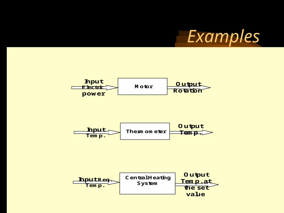
Examples
Motor Output Rotation
Input Electric power
Thermometer Output Temp.
Input Temp.
Central Heating System
Output Temp. at the set value
Input Req. Temp.

Stages of Dynamic System Investigation
• Physical Modeling
– Imagine a simple physical model that will match closely the behavior of the system
• Equations of Motion
– Develop Mathematical Model to describe the physical model
• Dynamic Behavior
– Study the dynamic behavior of the physical model
• Design Decisions
– choose physical parameters of the system such that it will behave as desired

Example


SCHEMATIC DIAGRAM OF HYDRO-POWERSTEERING SYSTEM
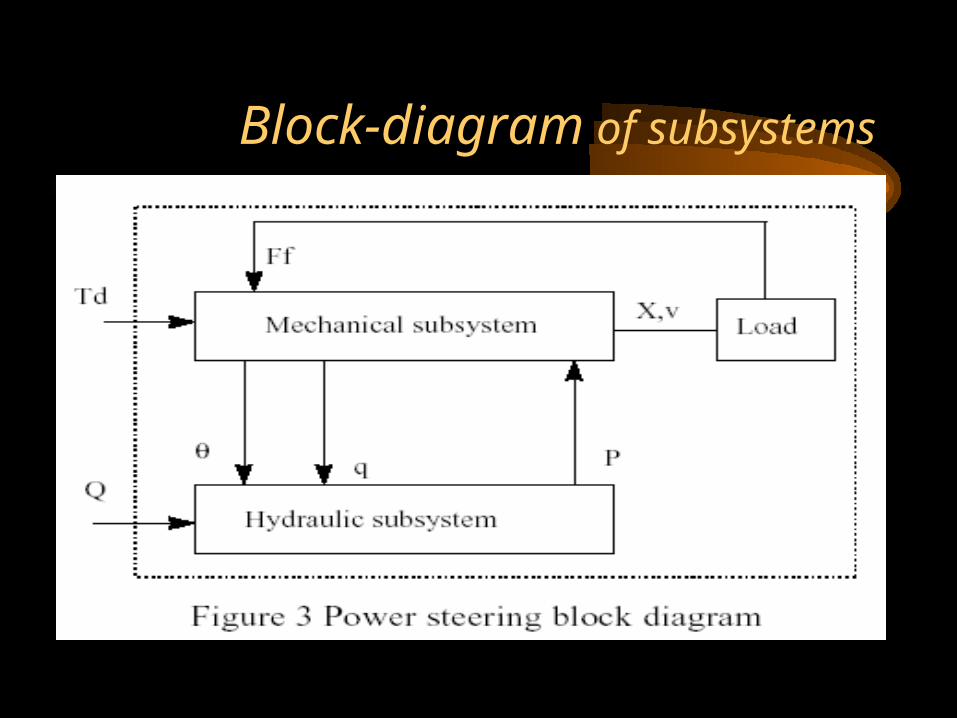
Block-diagram of subsystems

ALI KEYHANI MODEL : Mechanical subsystem
• The equations for the steering column, pinion and rack can be written :
Equation 1 :
Equation 2 :

ALI KEYHANI MODEL : Mechanical subsystem
Where Td=Torque generated by the driver,Theta1=rotational displacement for the steering column,
K2=tire stiffness
B2=Viscous damping coefficientB1=friction constant of the upper-steering column
X=displacement of the rack
m= mass of pinion
Ap= Piston area
K1=torsion bar stiffness
J1=Inertia constant of the upper steering column

ALI KEYHANI MODEL : Mechanical subsystem
The following assumptions were made :-the pressure forces on the spool are neglected.
-the stiffness of the steering column is infinite.
-the inertia of the lower steering column (valve spool and pinion) is lumped into the rack mass.

ALI KEYHANI MODEL hydraulic subsystem

ALI KEYHANI MODEL hydraulic subsystem
By applying the orifice equations to the rotary valve metering orifices and mass conservation equations to the entire hydraulic subsystem the following equation are
obtained :
Equation 1 :
Equation 2 :
Equation 3 :

ALI KEYHANI MODEL hydraulic subsystem
Where Ps and Po =supply and return pressure of the pump.
Pl and Pr = cylinder pressure on the left and right side.Q = supply flow rate of the pumpA1 and A2 are the metering orifice areaRho = density of the fluidBeta=bulk modulus of fluidL=length of the cylinderCd= discharge co-efficient

Approximations in Physical Modeling
Approximation Mathematical Simplification
Neglect small Effects Reduces number and complexity of differential equations
Assume environmentindependent of systemmotions
Reduces number and complexity of differential equations
Replace distributedcharacteristics by lumpedelements
Leads to ordinary rather than partial differentialequations
Assume linear relationships Makes equations linear (allows superposition ofSolutions)
Assume constantparameters
Leads to constant coefficients of diff. Eqns.
Neglect uncertainty andnoise
Avoids statistical treatment

Examples of approximations
• Neglect small effects
• Independent environment
• Lumped characteristics
• linear relationships
• constant parameters
• Neglect uncertainty and noise
• Realistic physical model leads to non-linear PDEs with time and space varying parameters
• Simplifying assumptions led to ODEs with constant coefficients
• Engineering Judgement is key!

From Physical Model to Mathematical Model
• Dynamic Equilibrium Relations: balance of forces, flow rates, energy, etc. which must exist for the system and sub-systems.
• Compatibility Relations: how motions of the system elements are interrelated because of the way they are interconnected.
• Physical Variables:Selection of precise physical variables (velocity, force, voltage, pressure, flow rate, etc.) with which to describe the instantaneous state of the system.

From Physical Model to Mathematical Model
• Physical Laws: Natural Physical laws which individual elements of the system obey, e.g. – Mechanical relations between force and motion
– electrical relations between current and voltage
– electromechanical relations between force and magnetic field
– thermodynamic relations between temperature, pressure, internal energy, etc.
– These are also called constitutive physical relationships!

Classification of Physical Variables
• Through Variables (one-point variables) measure the transmission of something through an element, e.g.– electric current through a resistor– fluid flow through a duct– force through a spring– heat flux flowing through

Classification of Physical Variables
• Across Variables (two-point variables) measures the difference in state between the ends of an element, e.g.– voltage drop across a resistor– pressure drop between the ends of a duct– difference in velocity between the ends of a
damper– temperature difference

Equilibrium Relations
• Are always relations among through variables– Kirchoff’s current law (at an electrical node)– continuity of fluid flow– equilibrium of forces meeting at a point– heat flux balance

Compatibility Relations
• Are always relations among “across variables”– Kirchoff’s voltage law around a circuit– pressure drop across all the connected stages of
a fluid system– geometric compatibility in a mechanical system

Physical Relations
• Are relations between through and across variables of each individual element, e.g.
• f = k.x for a spring
• I=V/R for a resistor

System Components
• spring • mass• damper• capacitor• Voltage generator• resistor• inductor
• Hydraulic valves• …..• A real system, may be
broken down into components that behave like one of the basic components

Mechanical Quantities
• F=force• T=torque• x=displacement angular
displacement dx/dt=v=velocity d/dt==angular
velocity
• dv/dt=a=acceleration• dw/dt==angular
acceleration • I=inertia• m=mass• k=spring constant• C=damping
coefficient

Electrical Quantities
• V=voltage
• Q=charge
• I=current
• L=inductance
• C=capacitance
• R=resistance

Building Blocks: Mechanical
• Translational:– spring; – F = kx (force displacement relationship), – E= 1/2(F2/k), energy stored
F

Building Blocks: Mechanical
• Translational: – dashpot (damper); – F = C v (C(dx/dt)) (Force-velocity relationship)– E = Cv 2 energy dissipated
F

Building Blocks: Mechanical
• Translational: – mass; – F = ma = m(d2x/dt2) – E = 1/2 mv2 , Kinetic Energy
F
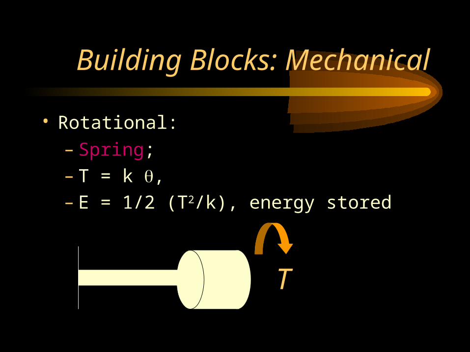
Building Blocks: Mechanical
• Rotational: – Spring; – T = k , – E = 1/2 (T2/k), energy stored
T

Building Blocks: Mechanical
• Rotational: – dashpot; – T = C = C d/dt – P = C2 energy dissipated
T

Building Blocks: Mechanical
• Rotational: – Moment of Intertia; – T = I d2 dt2
– E =1/2 I 2 , Kinetic energy
T

Building Blocks: Electrical
• Capacitor; • Q = CV or V = Q/C, • E = 1/2 CV2 energy stored
V

Building Blocks: Electrical
• Resistor; • V = IR or V = R (dQ/dt), • energy dissipated E = I2R
V

Building Blocks: Electrical
• Inductor; • V = L di/dt = L (d2Q/dt2) • E = 1/2 L I2 energy stored
V

Mechanical and Electrical Quantities
Symbol Mechanical Quantity Symbol Electrical Quantity
mI
massMoment of Inertia
L Inductance
k Spring Constant(linear and rotational)
1/C Reciprocal of Capacitance
C Damping Coeff. R Resistance
FT
ForceTorque
V Voltage
x
Translational motionRotational motion
Q Charge
dx/dtd/dt
Linear velocityAngular velocity
dQ/dt = i Current
d2x/dt2
d2 /dt2
Acceleration (linear)Acceleration (angular)
d2Q/dt2 Rate of change of current

Thermal System
• T = Temperature
• q = heat flux
• R=thermal resistance
• Conduction, R=L/Ak, A = cross-sectional area, L=length conducted over, k = thermal conductivity
• Convection, R=1/Ah, A = convective surface, h = convective heat transfer coefficient
• C=thermal capacitance, mCp (mass X specific heat capacity)

Thermal System
• q = (T2-T1)/R
• q=Ak(T2-T1)/L; conduction
• q=Ah(T2-T1); convection
• q1-q2=mCp(dT/dt), q1-q2= rate of change of internal energy

Hydraulic Systems
• We will not deal with Hydraulic systems here…...

Types of Systems
• Zeroth order systems
• First order systems
• Second order systems

Zeroth order systems

First -order systems: examples

First -order systems: examples

Example of a First order system
• Temperature measuring devices (e.g. thermocouple or a thermometer) are first-order systems.
• If a thermometer is dipped in a liquid:# mCp dT/dt = (Ak/L) (TL -T)
• where m = mass of bulb, Cp is the specific heat capacity, T is the current temperature of the mercury, A is the surface area of the bulb, k is its thermal conductivity, L is the wall thickness, and TL is the
temperature of the liquid.

First order system
• Rewritten:# mCp dT/dt + (Ak/L) T = (Ak/L) (TL)
• This is a first order system that has been subjected to a step input (which is the right hand side of the above equation)
• When this is integrated and initial conditions applied the solution of this system is an exponential function:
# T = TL + [T0-TL] e-t/

First order system
• T = TL + [T0-TL] e-t/
• T0 is the temperature of the bulb at intial time; andthe time constant, is written as (mCpL/Ak).
• Response of a First order system to a step input(decaying and progressing)
0
1
2
3
4
5
0 0.5 1
Series1
4.4
4.5
4.6
4.7
4.8
4.9
5
0 0.5 1
Series1

First order system
• Steady state value is TL (target).
• How soon is this value reached ? (imp. Question)• The answer lies in the magnitude of the time
constant (=mCpL/Ak, in this case).
• Time constant is defined as the time required to complete 63.2% of the process, i.e. if the temperature has to rise from 10 degrees to 70 degrees, time constant is the time required to reach (10 +63.2%of the interval) 47.92 degrees.
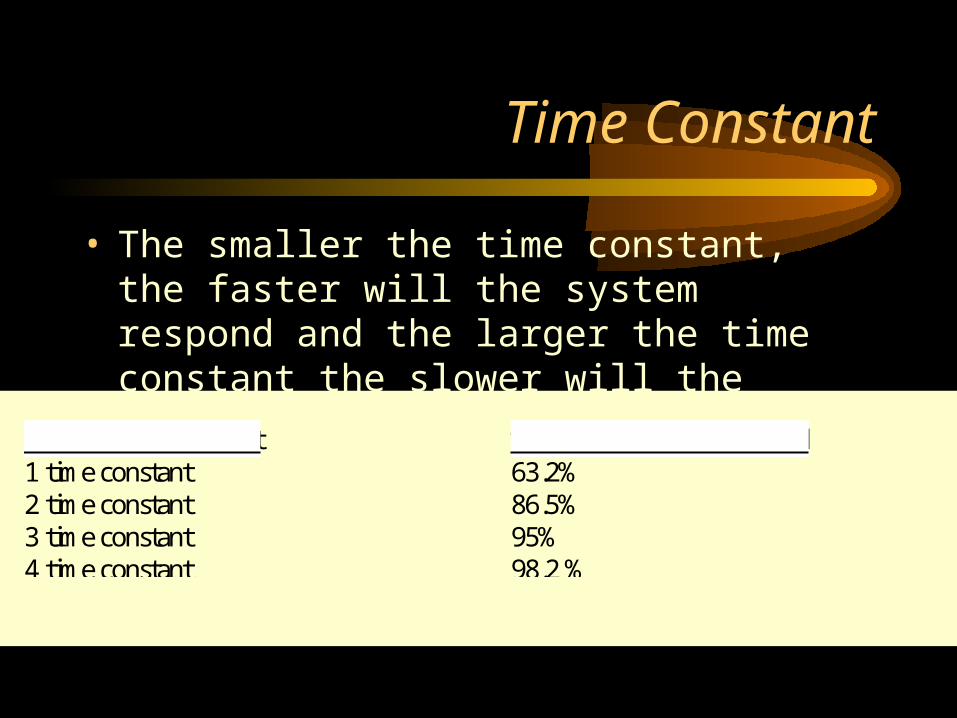
Time Constant
• The smaller the time constant, the faster will the system respond and the larger the time constant the slower will the system respond.
Amount of time spent % of the process completed 1 time constant 63.2%2 time constant 86.5%3 time constant 95%4 time constant 98.2 %

Second-order Systems: examples

Building a Mechanical System (spring-mass-dashpot)
• Newton’s Law:• F - kx -Cv = ma • F - kx - Cdx/dt =
m(d2x/dt2)• or m d2x/dt2 + Cdx/dt +
kx = F

Building an Electrical System (LRC Circuit)
• Kirchoff’s law• total current flowing
towards a junction =total current flowing out of a junction
• In a closed system sum of potential drops across each component =applied emf.
• L d2Q/dt2 + RdQ/dt + Q/C = Emf = V

Second order systems
• These are all second order systems since they are described by a second order differential equation.
• If the mass or the inductance is removed from the second order systems shown above they become first order systems.
• While such an electrical system makes sense the mechanical system without mass is unrealistic.

Second Order Systems
• m d2x/dt2 + Cdx/dt + kx = F• The solution has two components a CF and PI
• CF: Complementary function; solution with no F m d2x/dt2 + Cdx/dt + kx = 0
• PI: Particular Integral; solution with F; – m d2x/dt2 + Cdx/dt + kx = F
• PI is dictated by the nature of F

Finding CF
• Assuming the solution form to be x(t) = Aet
• (m2 + C+ k) Aet = 0 >> m2 + C+ k= 0
• Roots of the quadratic equation are:
• m
k
m
C
m
C
2
1 22
m
k
m
C
m
C
2
2 22

Finding CF
2221 nnn
2222 nnn
n )1( 21
n )1( 22
m
k
mk
C
m
k
mk
C
m
k )
4(
2
2
1
m
k
mk
C
m
k
mk
C
m
k )
4(
2
2
2
=damping ratio n=natural frequency

Finding CF….
• The solution takes a distinct form depending upon the values under the square-root sign
• When there is no damping in the system, C=0 (=0)and both the roots are imaginary
• solution:
• where A and B are constants determined from initial conditions x(0) and dx/dt (0)
)()( tm
kBSint
m
kACosxCF

Finding CF...
m
kn
• This motion represents pure undamped oscillatory motion with natural frequency of

Undamped System
-10
-5
0
5
10
0 2 4 6
Series1
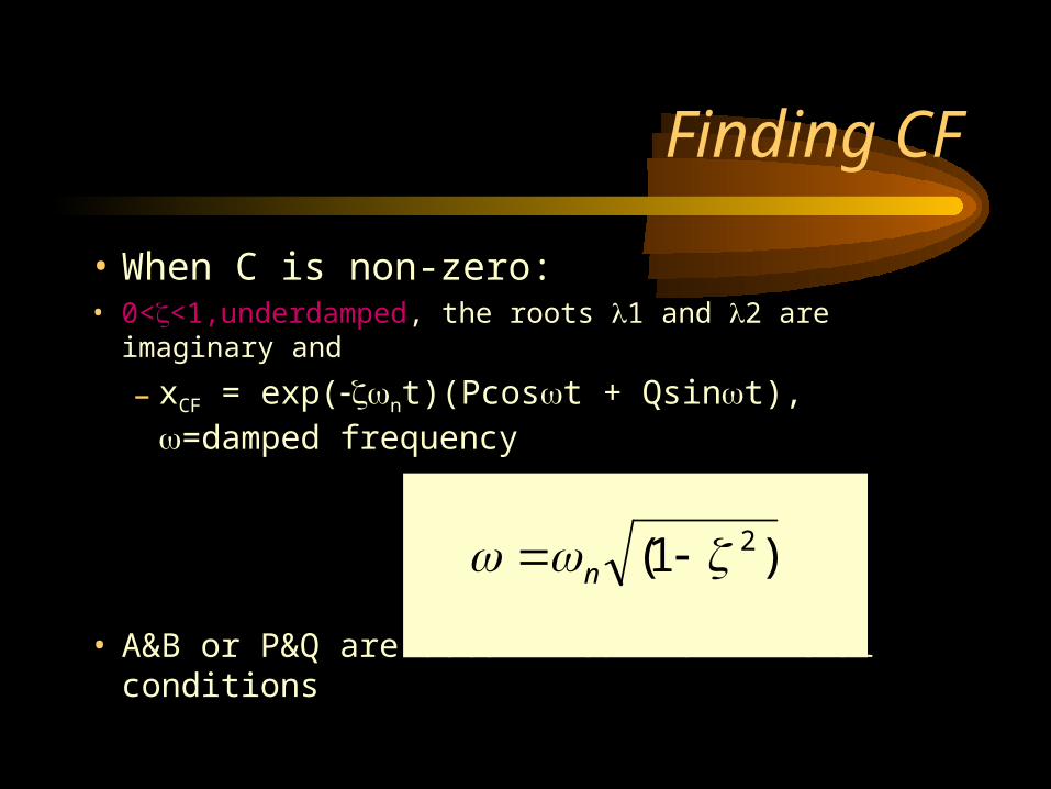
Finding CF
• When C is non-zero:• 0<<1,underdamped, the roots 1 and 2 are imaginary and
– xCF = exp(nt)(Pcost + Qsint), =damped frequency
• A&B or P&Q are determined from initial conditions
)1( 2 n

Underdamped System
-4
-2
0
2
4
6
8
0 2 4 6
Series1
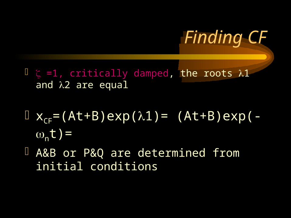
Finding CF
=1, critically damped, the roots 1 and 2 are equal
xCF=(At+B)exp(1)= (At+B)exp(-nt)= A&B or P&Q are determined from initial
conditions

Critically Damped System
00.5
11.5
22.5
33.5
4
0 2 4 6
Series1

Finding CF
>1, overdamped, roots the roots 1 and 2 are real and unequal
xCF=Aexp(1)+Bexp(2)
A&B or P&Q are determined from initial conditions

Finding PI: Interesting Questions!
• How do systems behave with time when subject to some disturbance ?
• How do systems behave when a certain input is provided ?
• What are some expected inputs?
• What do the outputs look like?

Response of Systems
• Natural response and Forced Response
• Natural: No input to the system (system acts on its own), e.g. water flowing out of a tank when a valve is kept open.
• Forced: water flowing out of a tank while there is input flow from another source.
• Transient and Steady State Response
• Transient: Response that dies after a short interval of time
• Steady State: Response that remains after all transient response died.

Second Order Systems
• m d2x/dt2 + Cdx/dt + kx = F• The solution has two components a CF and PI
• CF: Complementary function; solution with no F m d2x/dt2 + Cdx/dt + kx = 0
• PI: Particular Integral; solution with F; – m d2x/dt2 + Cdx/dt + kx = F
• PI is dictated by the nature of F

Step Input
• F is a step function
F
t

Response
• The solution mirrors the nature of the forcing function
• Therefore the particular integral is F/k
• So the total solution is the XCF +XPI
• XCF has different forms based on the nature of the system,
underdamped, critically damped, overdamped, etc.
• XPI is dependent on the forcing function

Step Response
• Rise time (tr): time taken to go from zero to steady state value
• Peak time (tp): time taken to hit first peak
• Overshoot: maximum amount by which system overshoots steady state value.
• Settling time (ts): time taken for oscillations to reach 2% of steady state.