Prof. Rajesh BhagatAsst. Professor

Civil Engineering Department

Yeshwantrao Chavan College Of Engineering

Nagpur

B. E. (Civil Engg.) M. Tech. (Enviro. Engg.)

GCOE, Amravati VNIT, Nagpur

Mobile No.:- 8483003474 / 8483002277

Email ID:- rajeysh7bhagat@gmail.com

Website:- www.rajeysh7bhagat.wordpress.com

ENGINEERING HYDROLOGY

UNIT-IV

Statistical Methods: Statistics in hydrological analysis, probability

and probability distribution.

Floods: Causes and effects, Factors affecting peak flows and its

estimation, Flood routing and Flood forecasting. Frequency analysis.

Economic planning for flood control.

Importance of Statistics and Probability in Hydrology:

1) If the outcome of a process can be precisely predicted is known as deterministic

process.

2) But in some cases, there is uncertainty or unpredictability regarding outcome.

3) Average weather condition are same from year to year, but yearly rainfall at a

given place is not same every year.

4) In all such a cases, process is treated as a probabilistic process and outcome

governed by some probability law.

Flood

1) Any flow which is relatively high and which overtops the natural or artificial

banks in any reach of a river may be called a flood.

2) Flood is the most worldwide natural disaster.

3) It occurs in every country and wherever there is rainfall or coastal hazards.

Different types of flood:-

Local flood:- caused due to high intensity of local rainfall which generate higher

surface run-off. Urbanization, Surface sealing and loss of infiltration capacity

increases the surface runoff causes local flood.

River floods: - River flood occur when the river volume exceeds due to excess of

run-off beyond the river capacity. The river levels rise slowly due to high intensity

rainfall for long lasting duration.

Flash floods:-Flash floods occur as a result of the rapid accumulation and release

of runoff waters from upstream mountainous areas, which can be caused by very

heavy rainfall, bursting of clouds, landslides, sudden break-up of an ice jam or

failure of flood control works.

Coastal floods:- High tides and storm caused by tropical depressions and cyclones

can cause coastal floods in urban areas, low-lying land near the sea in general.

Tidal effects can keep the river levels high for long periods of time and sustain

flooding.

Major parameters factors responsible for the occurrences of flood:

1) Climate:- Due to global warming or climate change many subsystems of the

global water cycle are effected causing an increase of flood magnitude as well as

flood frequency.

2) Nature of collecting basin:- A collecting basin is an area where surface water

from rain converges to a single point, it is usually exit of basin, where water

join another water body, such as a river. Larger the area of basin more will be the

water receiving capacity.

3) Nature of the streams: - Water flowing through a channel, such as a stream, has

the ability to transport sediment. Some percolates deep into the ground and

replenishes the groundwater supply.

4) Vegetative cover:- Trees reduce top soil erosion, prevent harmful land

pollutants contained in the soil from getting into our waterways, slow down

water run-off, and ensure that our groundwater supplies are continually being

replenished.

5) Rainfall: - It is difficult to predict and measure the precise changes in the

hydrological cycle because of the processes such as evaporation, transport, and

precipitation.

CAUSES OF FLOOD

1) Intense rainfall

2) Melting of snow

CAUSES OF FLOODING

1) Culvert, drain and gully entry blockage (partial or total)

Dumped rubbish.

Floating debris, including leaves and branches.

Sediment deposition

2) Poorly maintained urban watercourses (silted, overgrown with vegetation, or

blocked with rubbish.)

3) Bridge, culvert or tunnel waterway capacity exceeded.

4) Failure of drainage pump or jammed sluice gate.

5) High water level in receiving river that flows back up the drain or sewer.

FLOOD:-

1) Design of culvert, bridges, drainage work and irrigation diversion works, needs a

reliable estimates of the flood.

2) The maximum flood that any structure can safely pass is called the design flood.

3) As the magnitude of the design flood increase, the capital cost of the structure also

increases but the probability of annual damages will decrease.

4) Standard Project Flood (SPF) is the estimate of the flood likely to occur from the

most severe combination of the meteorological & hydrological conditions, which

are reasonably characteristics of the drainage basin being considered, but excluding

extremely rare combination.

5) Maximum Probable Flood (MPF) differs from the SPF in that it includes the

extremely rare and catastrophic floods and is usually confined to spillway design of

very high dams. The SPF is usually around 80% of the MPF for the basin.

DESIGN FLOOD:-

1) It is the flood adopted for the design of hydraulic structure like spillways, bridges,

flood banks, etc.

2) It may be MPF or SPF or flood of any desired recurrence interval.

3) The methods used in the estimation of the design flood can be grouped as under:

1) Physical indication of past flood

2) Envelop curves

3) Empirical flood formulae

4) Rational method

5) Unit hydrograph application

6) Frequency analysis or statistical method

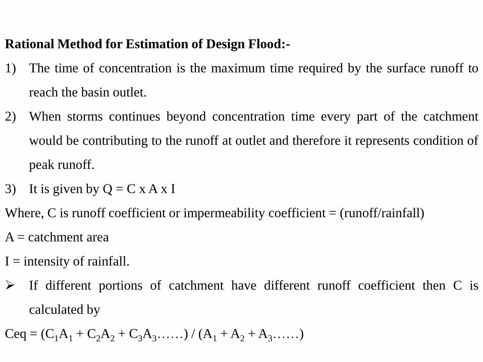
Rational Method for Estimation of Design Flood:-

1) The time of concentration is the maximum time required by the surface runoff to

reach the basin outlet.

2) When storms continues beyond concentration time every part of the catchment

would be contributing to the runoff at outlet and therefore it represents condition of

peak runoff.

3) It is given by Q = C x A x I

Where, C is runoff coefficient or impermeability coefficient = (runoff/rainfall)

A = catchment area

I = intensity of rainfall.

If different portions of catchment have different runoff coefficient then C is

calculated by

Ceq = (C1A1 + C2A2 + C3A3……) / (A1 + A2 + A3……)

Rational Method for Estimation of Design Flood:-

1) Q = C x A x I

2) The rational formula is found to be suitable for a peak flow prediction in small

catchment up to 50 km2 in area.

3) Application in urban drainage designs and in the design of small culverts and

bridges.

Rainfall Intensity, I tc,p = (KTx) / (tc + a)m

Probability exceedance P : (return period T = 1/P)

K, a, x and m are constant.

Kirpich Equation, tc = 0.01947 L0.77 S-0.358

tc = Time of concentration in minutes

L = Max. Length of traveller of water in meter

S = Slope of catchment = ∆H / L

∆H = Difference in elevation

12

What is a return period?

1) The probability that events such as floods, wind storms & earthquake will

occur is often expressed as a return period.

2) The inverse of probability (generally expressed in %), it gives the estimated

time interval between events of a similar size or intensity.

3) For example, the return period of a flood might be 100 years; otherwise

expressed as its probability of occurring being 1/100, or 1% in any one year.

This does not mean that if a flood with such a return period occurs, then the

next will occur in about one hundred years' time - instead, it means that, in

any given year, there is a 1% chance that it will happen, regardless of when

the last similar event was. Or, put differently, it is 10 times less likely to occur

than a flood with a return period of 10 years (or a probability of 10%).

13

What is a return period?

1) It represents the avg. number of years within which a given event will be

equaled or exceeded..

2) It is calculated by using Weibuls formula, T = (n + 1) / m

Where T is Return period, n is number of years in record & m is the order or

rank ( of highest observed flood)

1) After either the partial or annual series is complied, the items are arranged in

descending order of magnitude and assigned an order or rank, starting with 1

for the highest observed flood.

1) An urban catchment has an area of 0.85 km2. the slope of the catchment is 0.006 and the

maximum length of travel of water is 950 m. The maximum depth of rainfall with a 25 years

return period is as below:-

if culvert for drainage at the outlet of this area is to designed for a return period of 25 years,

estimates the required peak flow rate by assuming the runoff coefficient as 0.3.

Sol:- Time of concentration by Kirpich Equation, tc = 0.01947 L0.77 S-0.358

tc = 0.01947 x (9500.77 ) x (0.006)-0.358 = 27.4 minutes

Max. Depth of rainfall for 24.7 minute duration (by interpolation):

(50 - 40) / (30 - 20) = (50 - x) / (30 - 27.4)

x = 47.4 mm = max. Depth of rainfall for 27.4 minutes.

Avg intensity of rainfall = I tc,p = (47.4 / 27.4 ) 60 = 103.8 mm/hr

Q = C x A x I = (0.3 x 103.8 x 0.85 x 1000) / 60 x 60 = 7.35 m3 / s

Duration, Minute 5 10 20 30 40 60

Depth of rainfall, mm 17 26 40 50 57 62

2) If in the urban area, the land use of the area and the corresponding runoff

coefficient are as given below calculate the equivalent runoff coefficient.

Sol: Equivalent runoff coefficient

Ceq = (C1A1 + C2A2 + C3A3 + C4A4) / (A1 + A2 + A3 +A4)

Ceq = ((0.7x8) + (0.1x17) + (0.3x50) + (0.8x10)) / (8 + 17 + 50 +10)

= 0.36

Land Use Area (ha) Runoff coefficient

Roads 8 0.7

Lawn 17 0.1

Residential area 50 0.3

Industrial area 10 0.8

3) A small watershed consists of 1.5 km2 of cultivate area (C=0.2), 2.5 km2 under

forest (C=0.1) and 1.0 km2 under grass cover (C=0.35). There is a fall of 22 m in a

watercourse length of 1.8 km. The intensity frequency-duration relation for the

area may be taken as I = (80 x Tr0.2) / (tc + 13)0.46

Where I is in cm/hr, T is is in minutes. Estimate the peak rate of runoff for a 25

year frequency.

Sol: length of water course = 1.8 km = 1800 m & Fall in the elevation = 22 m

S = 22 / 1800 = 0.0122

tc = 0.0195 x (L0.77 ) x (S)-0.358

tc = 0.0195 x (18000.77 ) x (0.0122)-0.358 = 34 minutes

I = (80 x Tr0.2) / (tc + 13)0.46

I = (80 x 250.2) / (34 + 13)0.46 = 25.9 cm/hr

Ceq = (C1A1 + C2A2 + C3A3) / (A1 + A2 + A3)

Ceq = ((0.2x1.5) + (0.1x2.5) + (0.35x1)) / (1.5 + 2.5 + 1)

= 0.18

3) A small watershed consists of 1.5 km2 of cultivate area (C=0.2), 2.5 km2 under

forest (C=0.1) and 1.0 km2 under grass cover (C=0.35). There is a fall of 22 m in a

watercourse length of 1.8 km. The intensity frequency-duration relation for the

area may be taken as I = (80 x Tr0.2) / (tc + 13)0.46

Where I is in cm/hr, T is is in minutes. Estimate the peak rate of runoff for a 25

year frequency.

Sol:

S = 0.0122

Tc = 34 minutes

I = 25.9 cm/hr = 0.259 m / hr

Ceq = 0.18

Q = C x A x I = (0.18 x 5 x 1000000 x 0.259) / 60 x 60 = 64.75 m3 / s

4) A bridge is proposed to constant across a river having catchment area of 2027

hectors. The catchment has a slope of 0.007 and length of travel of water is

20270m. Estimates 30 years flood, the intensity frequency duration relationship is

given by

I = (9876 x Tr0.2) / (tc + 45)0.98

Where I is in mm/hr, Tr is in years & tc is in minutes. Assume runoff coefficient as

0.35.

Sol:- Time of concentration by Kirpich Equation, tc = 0.01947 L0.77 S-0.358

tc = 0.01947 x (202700.77 ) x (0.007)-0.358 = 272.45 minutes

Max. intensity of rainfall = I tc,p = ((9876 x 300.2 )) / ((272.45 + 45)0.98)

= 68.92 mm/hr = 6.892 cm/hr

A = 2027 Ha = 20.27 Km2

Q = C x A x I

Peak Discharge, Q = 2.78 x C x A x I = (2.78 x 0.35 x 6.892 x 20.27)

= 135.93 cumec

Estimation of Design Flood For A Particular Return Period:

1) The return period is calculated by using Weibull’s formula:

Tr = ( n + 1) / m

Tr = return period in years

n = number of years of record

m = order number

2) Return period represents the avg no. Of years within which a given event will be equalled

or exceeded. Probability of Exceedance, p = 1 / Tr

3) If the probability of occurrence of an event is p, then the probability of its no-occurrence

is q = 1- p

4) Probability of an event not occurring at all in ‘n’ successive years would be equal to qn

qn = (1- p)n

Probability of an event occurring at least once in ‘n’ successive years, = 1 – qn = 1- (1 - p)n

This probability is called risk.

A flood of a certain magnitude has a return period of 20 years. What is the probability

that a flood of this magnitude may occurs in next 15 years.

Return period represents the avg no. Of years within which a given event will be equalled or

exceeded. Probability of Exceedance, p = 1 / Tr

p = 1 / 20 = 0.05

Probability of an event not occurring at all in ‘n’ successive years would be equal to qn

qn = (1- p)n = (1 – 0.05)15 = 0.46

Probability of an event occurring at least once in ‘n’ successive years,

Risk = 1 – qn = 1- (1 - p)n

Risk = 1 – 0.46 = 0.54

The flood data analysis at river site yielded mean of 12000 m3/s & standard deviation of

650 m3/s for what discharge the structure should be designed so as to provide 95%

assurance that the structure will not fail in next 50 years.

Percentage of assurance = 95 %

Percentage risk = 5%

Risk = 1 – qn = 1- (1 - p)n

Probability of Exceedance, p = 1 / Tr

0.05 = 1- (1 - 1 / Tr)50

Tr = 975.286 years

YT = - ln ln (T / (T - 1)) = - ln ln (975.286 / (975.286 - 1)) =6.88

XT = X + K . σn-1 = 12000 + K . 650

K = Frequency factor = (YT – yn) / Sn = = (6.88 – 0.577) / 1.28225

XT = X + K . σn-1 = 12000 + K . 650

XT = 15195 m3/s

Estimation of Design Flood For A Particular Return Period:

1) The return period is calculated by using Weibull’s formula:

Tr = ( n + 1) / m

Tr = return period in years

n = number of years of record

m = order number

2) Return period represents the avg no. Of years within which a given event will be equalled

or exceeded. Probability of Exceedance = 1 / Tr = P

3) If a graph plotted between flood magnitude and its return period in simple plane co-

ordinates, the plot is called probability or empirical distribution. Extrapolation for large

return period may yield more result hence following method are used:

A. Gumble’s method

B. Log Pearson Type III Method

Gumble’s Method:

XT = X + K . σn-1

XT = value of flood magnitude of return period T years

X = mean value of past flood record = ( ∑X) / n = X

K = Frequency factor = (YT – yn) / Sn

YT = - ln ln (T / (T - 1))

No. Of years of records, n > 50 we use yn = 0.577 & Sn = 1.2825

σn-1 = Standard deviation = √ ( ( ∑ ( Xi – X )2 ) / ( n – 1 ) )

Gumble’s Probability Distribution Method for Prediction of Flood Peak:

1) This method of estimating the flood peak was given by Gumbel and is known as

Gumbel’s Distribution method.

2) This is a flood frequency method which is most widely used in hydrological analysis &

meteorological studies.

Procedure for Estimating Peak Flood:

1) From the given discharge data & for sample size n, X & Sx or σn are to be computed.

Sx OR σn-1 = Standard deviation = √ ( ( ∑ ( Xi – X )2 ) / ( n – 1 ) )

2) yn & σn are to be computed for given sample size, n.

(assumed if not given 0.577 & 1.28225)

1) For given Tr or T, YT is to be calculated by YT = - ln ln (T / (T - 1))

2) Frequency factor (K or KT) is calculated by K = (YT – yn) / Sn

3) Now the magnitude of flood XT can be obtained from XT = X + K . σn-1

Flood frequency computation for the river Chambal at Gandhisagar Dam by using

Gumble’s Method, yielded the following results:

Estimates the flood magnitude in this river with a return period of 500 years.

Sol: XT = X + K . σn-1

X100 = X + K100 . σn-1 & X50 = X + K50 . σn-1

X100 – X50 = (K100 - K50 ) σn-1

46300 – 40809 = (K100 - K50 ) σn-1

5491 = (K100 - K50 ) σn-1

Return Period, T (Years) Peak Flood, m3/s

50 40809

100 46300

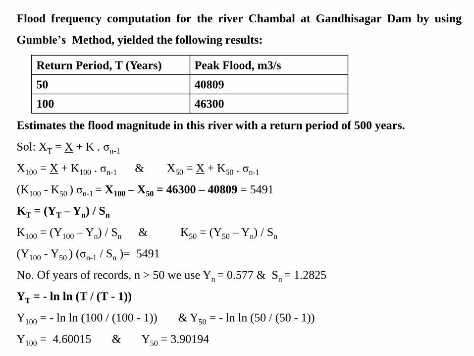
Flood frequency computation for the river Chambal at Gandhisagar Dam by using

Gumble’s Method, yielded the following results:

Estimates the flood magnitude in this river with a return period of 500 years.

Sol: XT = X + K . σn-1

X100 = X + K100 . σn-1 & X50 = X + K50 . σn-1

(K100 - K50 ) σn-1 = X100 – X50 = 46300 – 40809 = 5491

KT = (YT – Yn) / Sn

K100 = (Y100 – Yn) / Sn & K50 = (Y50 – Yn) / Sn

(Y100 - Y50 ) (σn-1 / Sn )= 5491

No. Of years of records, n > 50 we use Yn = 0.577 & Sn = 1.2825

YT = - ln ln (T / (T - 1))

Y100 = - ln ln (100 / (100 - 1)) & Y50 = - ln ln (50 / (50 - 1))

Y100 = 4.60015 & Y50 = 3.90194

Return Period, T (Years) Peak Flood, m3/s

50 40809

100 46300

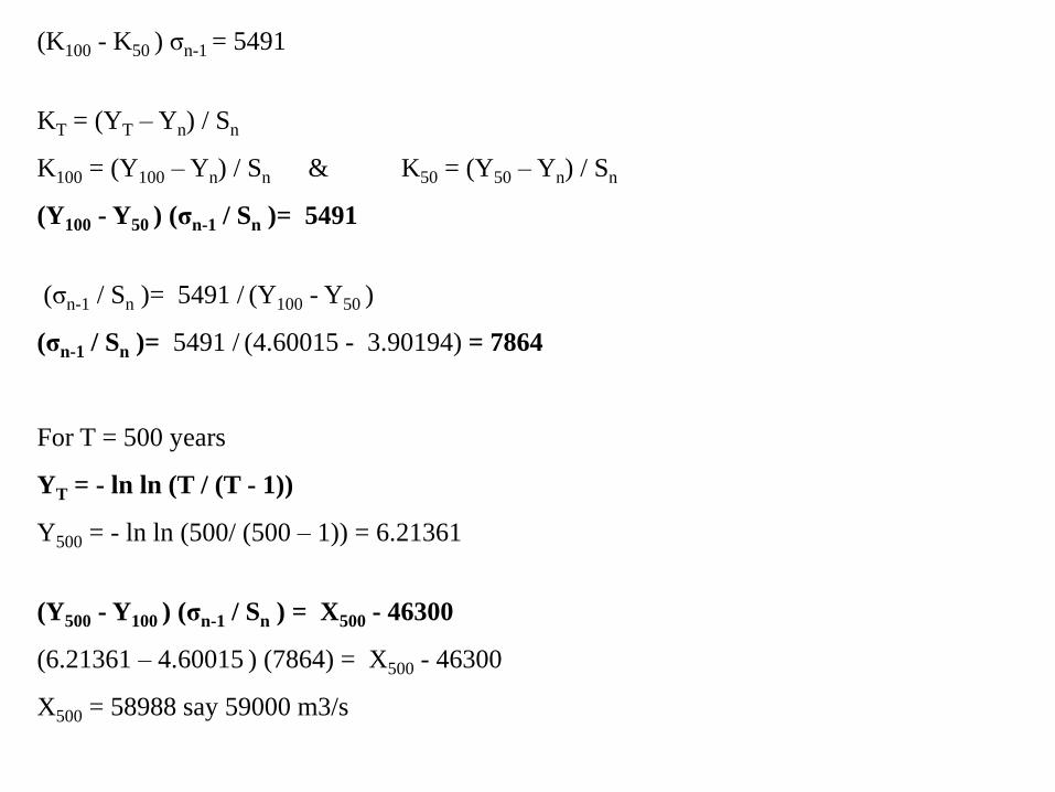
(K100 - K50 ) σn-1 = 5491

KT = (YT – Yn) / Sn

K100 = (Y100 – Yn) / Sn & K50 = (Y50 – Yn) / Sn

(Y100 - Y50 ) (σn-1 / Sn )= 5491

(σn-1 / Sn )= 5491 / (Y100 - Y50 )

(σn-1 / Sn )= 5491 / (4.60015 - 3.90194) = 7864

For T = 500 years

YT = - ln ln (T / (T - 1))

Y500 = - ln ln (500/ (500 – 1)) = 6.21361

(Y500 - Y100 ) (σn-1 / Sn ) = X500 - 46300

(6.21361 – 4.60015 ) (7864) = X500 - 46300

X500 = 58988 say 59000 m3/s

Flood Routing:-

1) It is the technique of determining the flood hydrograph at a section of a river by utilising

the data of flood flow at one or more upstream sections.

2) It is also used in analysis of a flood forecasting, flood protection, reservoir design,

spillway design etc.

3) The broad categories of flood routing are reservoir routing and channel routing.

4) In reservoir routing the effect of reservoir storage on a flood hydrograph is analysed.

This is used in design, location and sizing of the capacity of reservoir.

5) In channel routing the effect of storage of a specified channel reach on the flood

hydrograph is studied. It is used in flood forecasting and flood protection.

30

31

32

33

34

35