Engineering Highway Hierarchies

Peter Sanders and Dominik Schultes

Universitat Karlsruhe (TH), 76128 Karlsruhe, Germany,{sanders,schultes}@ira.uka.de

Abstract. Highway hierarchies exploit hierarchical properties inherent in real-world road networks toallow fast and exact point-to-point shortest-path queries. A fast preprocessing routine iteratively performstwo steps: first, it removes edges that only appear on shortest paths close to source or target; second, itidentifies low-degree nodes and bypasses them by introducing shortcut edges. The resulting hierarchy ofhighway networks is then used in a Dijkstra-like bidirectional query algorithm to considerably reduce thesearch space size without losing exactness. The crucial fact is that ‘far away’ from source and target it issufficient to consider only high-level edges.Various experiments with real-world road networks confirm the performance of our approach. On a 2.0 GHzmachine, preprocessing the network of Western Europe, which consists of about 18 million nodes, takes13 minutes and yields 48 bytes of additional data per node. Then, random queries take 0.61 ms on average.If we are willing to accept slower query times (1.10 ms), the memory usage can be decreased to 17 bytesper node. We can guarantee that at most 0.014% of all nodes arevisited during any query. Results for USroad networks are similar.Highway hierarchies can be combined with goal-directed search, they can be extended to answer many-to-many queries, and they are a crucial ingredient for otherspeedup techniques, namely for transit-noderouting and highway-node routing.

1 Introduction

Computing fastest routes in road networks from a given source to a given target location isone of the showpieces of real-world applications of algorithmics. Many people frequentlyuse this functionality when planning trips with their cars.There are also many applicationslike logistic planning or traffic simulation that need to solve a huge number of shortest-pathqueries. In principle we could use Dijkstra’s algorithm [1]. But for large road networks thiswould be far too slow. Therefore, there is considerable interest in speedup techniques forroute planning. Most approaches, including ours, assume that the road network isstatic,i.e., it does not change very often. Then, we can allow some preprocessing that generatesauxiliary data that can be used to accelerate all subsequentqueries. The preprocessing shouldbe sufficiently fast to deal even with very large road networks, the auxiliary data shouldoccupy only a moderate amount of space, and the queries should be as fast as possible.

1.1 Related Work

A detailed overview on shortest-path speedup techniques can be found in [2].

Bidirectional Search.A classical technique isbidirectional searchwhich simultaneouslysearches forward from the source and backwards from the target until the search frontiersmeet. Many more advanced speedup techniques use bidirectional search as an ingredient.

Goal Direction. Road networks allow effective goal-directed search usingA∗ search[3]:lower bounds define a vertex potential that directs search towards the target. This approachwas recently shown to be very effective if lower bounds are computed using precomputedshortest-path distances to a carefully selected set of about 20 Landmarknodes [4, 5] usingtheTriangle inequality (ALT).

The Precomputed Cluster Distances (PCD) technique [6] alsouses precomputed dis-tances for goal-directed search, yielding speedups comparable to ALT, but using less space.

The network is partitioned into clusters and the shortest connection between any pair ofclusters is precomputed. Then, during a query, upper and lower bounds can be derived thatcan be used to prune the search.

Another goal-directed approach is to precompute for each edge ‘signposts’ that supportthe decision whether the target can possibly be reached on a shortest path via this edge.During a query only promising edges have to be considered. Various instantiations of thisgeneral idea have been presented [7–13]. While these methods exhibit good query perfor-mance, preprocessing times are quite large and so far no experimental results for the largestpublicly available road networks have been published.

Separators.Perhaps the most well known property of road networks is thatthey are al-most planar, i.e, techniques developed for planar graphs will often also work for road net-works. Queries accurate within a factor(1 + ǫ) can be answered in near constant time us-ing O((n log n)/ǫ) space and preprocessing time [14]. Recently, this approachhas beenefficiently implemented and experimentally evaluated on a road network with one millionnodes [15]. While the query times are very good (less than 20µs for ǫ = 0.01), the pre-processing time and space consumption are quite high (2.5 hours and 2 GB, respectively).UsingO(n log3 n) space and preprocessing time, query timeO(

√n log n) can be achieved

[16] for directed planar graphs without negative cycles.Another previous approach is theseparator-based multi-level method[7, 17]. The idea is

to use a set of nodesV1 whose removal partitions the graphG = G0 into small components.Now consider theoverlay graphG1 = (V1, E1) where edges inE1 areshortcutscorrespond-ing to shortest paths inG that do not have inner nodes that belong toV1. Routing can nowbe restricted toG1 and the components containings and t respectively. This process canbe iterated yielding a multi-level method. A limitation of this approach is that the graphsat higher levels become much more dense than the input graphs, thus limiting the benefitsgained from the hierarchy. Also, computing small separators can become quite costly forlarge graphs.

Reach-Based Routing / REAL.Let R(v) := maxs,t∈V Rst(v) denote thereachof nodevwhereRst(v) := min(d(s, v), d(v, t)). Gutman [18] observed that a shortest-path search canbe stopped at nodes with a reach too small to get to source or target from there. Goldberg etal. [19, 20] have considerably strengthened this approach by introducing various improve-ments, in particular a combination with ALT, yielding theREAL algorithm. Its query per-formance is similar to our highway hierarchies, while the preprocessing times are usuallyworse; a comparison can be found in Section 6.7.

Heuristics. In the last decades, commercial navigation systems were developed which had tohandle ever more detailed descriptions of road networks on rather low-powered processors.Vendors resolved to heuristics still used today that do not give any performance guarantees:A∗ search with estimates on the distance to the target rather than lower bounds or heuristichierarchical approaches [21, 22].

1.2 Our Contributions

Our exacthighway hierarchies (first published in [23, 24]) are inspired byheuristichier-archical approaches. It is a bidirectional technique. While the search is inside some localarea around source or target, all roads of the network are considered. Outside these areas,however, the search is restricted to ‘important’ roads. This general idea can be iterated and

2

applied to a hierarchy consisting of several levels. The crucial point is the definition of ‘im-portant streets’. In previous heuristic variants, this definition is based on a classificationof the streets according to their type (motorway, national road, regional road,. . .). Such aclassification requires manual tuning of the data and a delicate trade-off between speed andsuboptimality of the computed routes. In our exact variant,however, nodes and edges areclassified fully automatically in a preprocessing step in such a way that all shortest paths arepreserved. By this means, we win not only exactness, but alsogreater speed since we canbuild high-performance hierarchies consisting of many levels without worrying about thequality of the results.

In the preprocessing phase, we alternate between two procedures: edge reduction andnode reduction.Edge reductionremoves non-highway edges, i.e., edges that only appear onshortest paths close to source or target. More specifically,every nodev has a neighbourhoodradiusr(v) we are free to choose. An edge(u, v) is a highway edge if it belongs to someshortest path from a nodes to a nodet such that(u, v) is neither fully contained in theneighbourhood ofs nor in the neighbourhood oft, i.e.,d(s, v) > r(s) andd(u, t) > r(t). Inall our experiments, neighbourhood radii are chosen such that each neighbourhood containsa certain numberH of nodes.H is a tuning parameter that can be used to control the rate atwhich the network shrinks.

Node reduction(also calledcontraction) removes low degree nodes by bypassing themwith newly introduced shortcut edges. In particular, all nodes of degree one and two areremoved by this process.

The query algorithm is very similar to bidirectional Dijkstra search with the differencethat certain edges need not be expanded when the search is sufficiently far from source ortarget. Highway hierarchies are the first speedup techniquethat was able handle the largestavailable road networks giving query times measured in milliseconds. There are two mainreasons for this success: Under the above reduction routines, the road network shrinks ina geometric fashion from level to level and remains sparse and near planar, i.e., levels ofthe highway hierarchy are in some senseself similar. The other key property is that prepro-cessing can be done using limited local searches starting from each node. Preprocessing isalso the most nontrivial aspect of highway hierarchies. In particular, long edges (e.g. long-distance ferry connections) make simple minded approachesfar too slow. Instead we usefast heuristics that compute a superset of the set of highwayedges.

Some further optimisations allow to drop the average query times below one millisecondon a 2.0 GHz machine—even for a road network with more than 30 million nodes. One ofthese optimisations is an all-pairs distance table that we precompute for the topmost levelLso that forward and backward search can be stopped as soon as all entrance points to levelLhave been found. Then, the remaining gap can be bridged by performing a moderate numberof simple table lookups.

We cannot give a general worst-case bound better than Dijkstra’s. So far, this drawbackapplies to all other exact speedup techniques, where an implementation is available, as well.However, in contrast to most of them, we can provideper-instance worst-case guarantees,i.e., for a given graph, we can determine an upper bound for the search space size ofanypossible point-to-point query performing only a linear number of unidirectional highwayqueries.

1.3 Subsequent Work

Various other speedup techniques were inspired by our highway hierarchies or even use themas their starting point. Goldberg et al. adopted the introduction of shortcuts in order to im-

3

prove both preprocessing and query times of the REAL algorithm. There is a many-to-manyvariant [25] and a combination with ALT [26]. Furthermore, the fastest implementation oftransit-node routing [27, 28] allowing query times of a few microseconds is also based onour highway hierarchies. The same applies to highway-node routing [29], a very recentapproach that can be used to handle dynamic scenarios, traffic jams for example. An alter-native, heuristic approach to dealing with dynamic scenarios, which is based on highwayhierarchies as well, has been developed by Nannicini et al. [30].

1.4 Outline

After beginning with some preliminaries in Section 2, we formally define thehighway hi-erarchyof a given graph in Section 3. Then, Section 4 deals with both procedures of thepreprocessing phase, the edge reduction (i.e., theconstructionof a highway network) andthe node reduction (i.e., thecontractionof a highway network). The basic query algorithmis introduced in Section 5. Furthermore, several optimisations are presented and some ad-vanced topics, like outputting complete path descriptionsand dealing with turning restric-tions, are discussed. In Section 6, we present a wide range ofexperimental results, dealingwith various real-world road networks, parameter settings, and scenarios of application. Wedo not only give average query times, but also a detailed analysis of queries with differ-ent degrees of difficulty, per-instance worst-case upper bounds, and comparisons to otherspeedup techniques.

2 Preliminaries

Graphs and Paths.We expect adirectedgraphG = (V, E) with n nodes andm edges(u, v)with nonnegativeweightsw(u, v) as input. Thelength w(P ) of a pathP is the sum ofthe weights of the edges that belong toP . P ∗ = 〈s, . . . , t〉 is a shortest pathif there isno pathP ′ from s to t such thatw(P ′) < w(P ∗). The distanced(s, t) betweens and tis the length of a shortest path froms to t or ∞ if there is no path froms to t. If P =〈s, . . . , s′, u1, u2, . . . , uk, t

′, . . . , t〉 is a path froms to t, thenP |s′→t′ = 〈s′, u1, u2, . . . , uk, t′〉

denotes thesubpathof P from s′ to t′. We useu ≺P v to denote that a nodeu precedes1 anodev on a pathP = 〈. . . , u, . . . , v, . . .〉; we just writeu ≺ v if the pathP that is referredto is clear from the context.

Dijkstra’s Algorithm.Dijkstra’s algorithm [1] can be used to solve thesingle-source shortest-path (SSSP) problem, i.e., to compute the shortest paths from a single source node s to allother nodes in a given graph. It is covered by virtually any textbook on algorithms, e.g. [31,32], so that we confine ourselves to introducing our terminology: Starting with the sourcenodes as root, Dijkstra’s algorithm grows ashortest-path treethat contains shortest pathsfrom s to all other nodes. During this process, each node of the graph isunreached, reached,or settled. A node that already belongs to the tree issettled. If a nodeu is settled, a shortestpathP ∗ from s to u has been found and the distanced(s, u) = w(P ∗) is known. A node thatis adjacent to a settled node isreached. Note that a settled node is also reached. If a nodeuis reached, a pathP from s to u, which might not be the shortest one, has been found anda tentative distanceδ(u) = w(P ) is known. A nodeu that is not reached isunreached; forsuch a node, we haveδ(u) =∞.

In case that the shortest paths in a graph are not unique, Dijkstra’s algorithm can beeasily modified to determineall shortest paths betweens and any nodeu ∈ V . This meansthat not a shortest-path tree is grown, but a shortest-pathdirected acyclic graph(DAG).

1 This doesnot necessarily mean thatu is thedirect predecessor ofv.

4

A bidirectionalversion of Dijkstra’s algorithm can be used to find a shortestpath from agiven nodes to a given nodet. Two Dijkstra searches are executed in parallel: one searchesfrom the source nodes in the original graphG = (V, E), also calledforward graphanddenoted as

−→G = (V,

−→E ); another searches from the target nodet backwards, i.e., it searches

in thereverse graph←−G = (V,

←−E ),←−E := {(v, u) | (u, v) ∈ E}. The reverse graph

←−G is also

calledbackward graph. When both search scopes meet, a shortest path froms to t has beenfound.

3 Highway Hierarchy

A highway hierarchyof a graphG consists of several levelsG0, G1, G2, . . . , GL, where thenumber of levelsL + 1 is given. We will provide an inductive definition of the levels:

– Base case (G′0, G0): level 0 (G0 = (V0, E0)) corresponds to the original graphG; fur-thermore, we defineG′0 := G0.

– First step (G′ℓ → Gℓ+1, 0 ≤ ℓ < L): for givenneighbourhood radii, we will define thehighway networkGℓ+1 of a graphG′ℓ.

– Second step (Gℓ → G′ℓ, 1 ≤ ℓ ≤ L): for a given setBℓ ⊆ Vℓ of bypassablenodes, wewill define thecoreG′ℓ of levelℓ.

First step (highway network). For each nodeu, we choose nonnegativeneighbourhoodradii r→ℓ (u) andr←ℓ (u) for the forward and backward graph, respectively. To avoid somecase distinctions, we setr→ℓ (u) andr←ℓ (u) to infinity for u 6∈ V ′ℓ (Radius Property R1) andfor ℓ = L (R2). In all other cases, neighbourhood radii have to be6=∞ (R3).

The level-ℓ neighbourhoodof a nodeu ∈ V ′ℓ isN→ℓ (u) := {v ∈ V ′ℓ | dℓ(u, v) ≤ r→ℓ (u)}with respect to the forward graph and, analogously,N←ℓ (u) := {v ∈ V ′ℓ | d←ℓ (u, v) ≤r←ℓ (u)} with respect to the backward graph, wheredℓ(u, v) denotes the distance fromu to v

in the forward graphGℓ andd←ℓ (u, v) := dℓ(v, u) in the backward graph←−Gℓ.

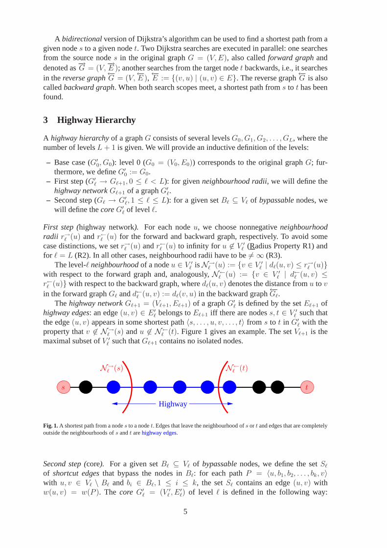
Thehighway networkGℓ+1 = (Vℓ+1, Eℓ+1) of a graphG′ℓ is defined by the setEℓ+1 ofhighway edges: an edge(u, v) ∈ E ′ℓ belongs toEℓ+1 iff there are nodess, t ∈ V ′ℓ such thatthe edge(u, v) appears in some shortest path〈s, . . . , u, v, . . . , t〉 from s to t in G′ℓ with theproperty thatv 6∈ N→ℓ (s) andu 6∈ N←ℓ (t). Figure 1 gives an example. The setVℓ+1 is themaximal subset ofV ′ℓ such thatGℓ+1 contains no isolated nodes.

N←ℓ (t)N→ℓ (s)

s t

Highway

Fig. 1.A shortest path from a nodes to a nodet. Edges that leave the neighbourhood ofs or t and edges that are completelyoutside the neighbourhoods ofs andt arehighway edges.

Second step (core). For a given setBℓ ⊆ Vℓ of bypassablenodes, we define the setSℓ

of shortcut edgesthat bypass the nodes inBℓ: for each pathP = 〈u, b1, b2, . . . , bk, v〉with u, v ∈ Vℓ \ Bℓ and bi ∈ Bℓ, 1 ≤ i ≤ k, the setSℓ contains an edge(u, v) withw(u, v) = w(P ). The core G′ℓ = (V ′ℓ , E

′ℓ) of level ℓ is defined in the following way:

5

V ′ℓ := Vℓ \ Bℓ andE ′ℓ := (Eℓ ∩ (V ′ℓ × V ′ℓ )) ∪ Sℓ. This definition is illustrated in Figure 2.Removing all core nodes fromGℓ yields connectedcomponents of bypassed nodes.

The level ℓ(e) of an edgee is max{ℓ | e ∈ Eℓ ∪ Sℓ}. For an edge(u, v), we usuallywrite justℓ(u, v) instead ofℓ((u, v)). The highway hierarchy can be interpreted as a singlegraphG := (V, E ∪⋃L

i=1 Si) where each node and each edge has additional information onits membership in the various setsVℓ, V

′ℓ , Bℓ, Eℓ, E

′ℓ, Sℓ.

contracted network ("core")= non−bypassed nodes+ shortcuts

bypassednodes

Fig. 2. The core of a highway network consists of the subgraph induced by the set of non-bypassed nodes and additionalshortcut edges.

4 Construction

4.1 Computing the Highway Network

Neighbourhood Radii.Let us fix any rule that decides which element Dijkstra’s algorithmremoves from the priority queue in the case that there is morethan one queued element withthe smallest key. Then, during a Dijkstra search from a givennodeu, all nodes are settledin a fixed order. TheDijkstra rank rku(v) of a nodev is the rank ofv w.r.t. this order.u hasDijkstra rank rku(u) = 0, the closest neighbourv1 of u has Dijkstra rank rku(v1) = 1, andso on.

We suggest the following strategy to set the neighbourhood radii. For this paragraph, weinterpret the graphG′ℓ as an undirected graph, i.e., a directed edge(u, v) is interpreted asan undirected edge{u, v} even if the edge(v, u) does not exist in the directed graph. Letd↔ℓ (u, v) denote the distance between two nodesu andv in the undirected graph. For a givenparameterHℓ, for any nodeu ∈ V ′ℓ , we setr→ℓ (u) := r←ℓ (u) := d↔ℓ (u, v), wherev is thenode whose Dijkstra rank rku(v) (w.r.t. the undirected graph) isHℓ. For any nodeu 6∈ V ′ℓ ,we setr→ℓ (u) := r←ℓ (u) :=∞ (to fulfil R1).

Originally, we wanted to apply the above strategy to the forward and backward graph oneafter the other in order to define the forward and backward radius, respectively. However, itturned out that using the same value for both forward and backward radius yields a similargood performance, but needs only half the memory.

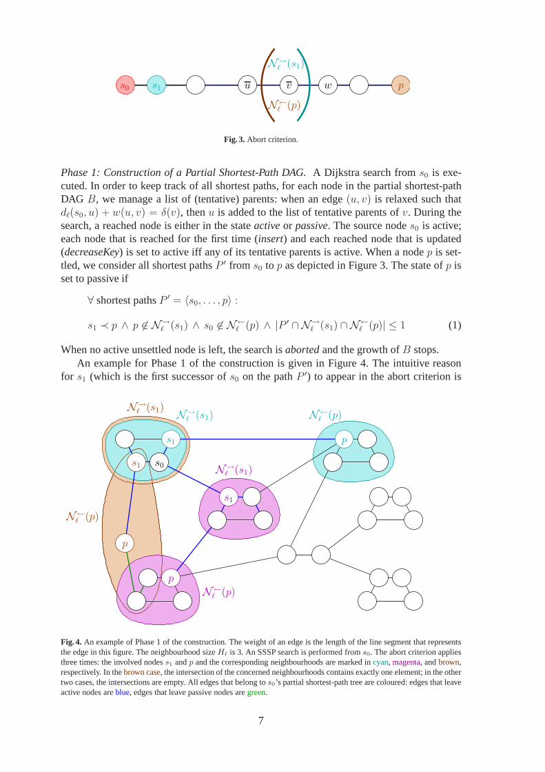
Fast Construction: Outline.Given a graphG′ℓ, we want to construct a highway networkGℓ+1. We start with an empty set of highway edgesEℓ+1. For each nodes0 ∈ V ′ℓ , twophases are performed: the forward construction of a partialshortest-path DAGB (containingall shortest paths froms0 to any nodeu ∈ B) and the backward evaluation ofB. Theconstruction is done by an SSSP search froms0; during the evaluation phase, paths fromthe leaves ofB to the roots0 are traversed and for each edge on these paths, it is decidedwhether to add it toEℓ+1 or not. The crucial part is the specification of an abort criterion forthe SSSP search in order to restrict it to a ‘local search’.

6

N→ℓ (s1)

N←ℓ (p)

s0 s1 pu v w

Fig. 3. Abort criterion.

Phase 1: Construction of a Partial Shortest-Path DAG.A Dijkstra search froms0 is exe-cuted. In order to keep track of all shortest paths, for each node in the partial shortest-pathDAG B, we manage a list of (tentative) parents: when an edge(u, v) is relaxed such thatdℓ(s0, u) + w(u, v) = δ(v), thenu is added to the list of tentative parents ofv. During thesearch, a reached node is either in the stateactiveor passive. The source nodes0 is active;each node that is reached for the first time (insert) and each reached node that is updated(decreaseKey) is set to active iff any of its tentative parents is active. When a nodep is set-tled, we consider all shortest pathsP ′ from s0 to p as depicted in Figure 3. The state ofp isset to passive if

∀ shortest pathsP ′ = 〈s0, . . . , p〉 :

s1 ≺ p ∧ p 6∈ N→ℓ (s1) ∧ s0 6∈ N←ℓ (p) ∧ |P ′ ∩ N→ℓ (s1) ∩ N←ℓ (p)| ≤ 1 (1)

When no active unsettled node is left, the search isabortedand the growth ofB stops.An example for Phase 1 of the construction is given in Figure 4. The intuitive reason

for s1 (which is the first successor ofs0 on the pathP ′) to appear in the abort criterion is

s1

s0s1

p

s1

p

p

18

1716

22

19

23

20 21

14

13

15

2524

10

9

11

67

4

0

N→ℓ (s1)N→ℓ (s1)

N→ℓ (s1)

N←ℓ (p)

N←ℓ (p)

N←ℓ (p)

Fig. 4. An example of Phase 1 of the construction. The weight of an edge is the length of the line segment that representsthe edge in this figure. The neighbourhood sizeHℓ is 3. An SSSP search is performed froms0. The abort criterion appliesthree times: the involved nodess1 andp and the corresponding neighbourhoods are marked incyan, magenta, andbrown,respectively. In thebrown case, the intersection of the concerned neighbourhoods contains exactly one element; in the othertwo cases, the intersections are empty. All edges that belong tos0’s partial shortest-path tree are coloured: edges that leaveactive nodes areblue, edges that leave passive nodes aregreen.

7

the following: When we deactivate a nodep during the search froms0, we decide to ignoreeverything that lies behindp. We are free to do this because the abort criterion ensures thats1 can take ‘responsibility’ for the things that lie behindp, i.e., further important edges willbe added during the search froms1. (Of course,s1 will refer a part of its ‘responsibility’ toits successor, and so on.)

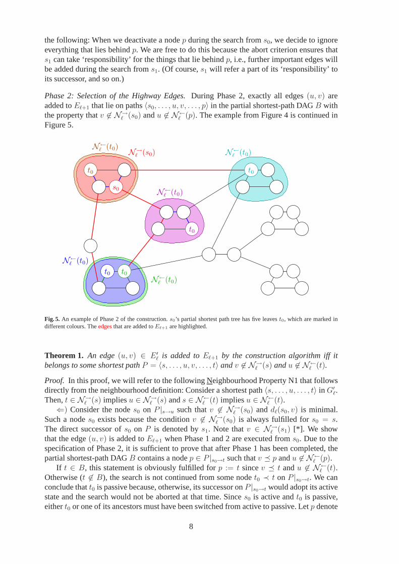
Phase 2: Selection of the Highway Edges.During Phase 2, exactly all edges(u, v) areadded toEℓ+1 that lie on paths〈s0, . . . , u, v, . . . , p〉 in the partial shortest-path DAGB withthe property thatv 6∈ N→ℓ (s0) andu 6∈ N←ℓ (p). The example from Figure 4 is continued inFigure 5.

.

s0.

t0

.

t0

p

18

1716

22

19

23

20 21

14

13

15

2524

9

11

67

t0

t0

t0

N→ℓ (s0)N←ℓ (t0)

N←ℓ (t0)

N←ℓ (t0)

N←ℓ (t0)

N←ℓ (t0)

Fig. 5. An example of Phase 2 of the construction.s0’s partial shortest path tree has five leavest0, which are marked indifferent colours. Theedgesthat are added toEℓ+1 are highlighted.

Theorem 1. An edge(u, v) ∈ E ′ℓ is added toEℓ+1 by the construction algorithm iff itbelongs to some shortest pathP = 〈s, . . . , u, v, . . . , t〉 andv 6∈ N→ℓ (s) andu 6∈ N←ℓ (t).

Proof. In this proof, we will refer to the following Neighbourhood Property N1 that followsdirectly from the neighbourhood definition: Consider a shortest path〈s, . . . , u, . . . , t〉 in G′ℓ.Then,t ∈ N→ℓ (s) impliesu ∈ N→ℓ (s) ands ∈ N←ℓ (t) impliesu ∈ N←ℓ (t).⇐) Consider the nodes0 on P |s→u such thatv 6∈ N→ℓ (s0) anddℓ(s0, v) is minimal.

Such a nodes0 exists because the conditionv 6∈ N→ℓ (s0) is always fulfilled fors0 = s.The direct successor ofs0 on P is denoted bys1. Note thatv ∈ N→ℓ (s1) [*]. We showthat the edge(u, v) is added toEℓ+1 when Phase 1 and 2 are executed froms0. Due to thespecification of Phase 2, it is sufficient to prove that after Phase 1 has been completed, thepartial shortest-path DAGB contains a nodep ∈ P |s0→t such thatv � p andu 6∈ N←ℓ (p).

If t ∈ B, this statement is obviously fulfilled forp := t sincev � t andu 6∈ N←ℓ (t).Otherwise (t 6∈ B), the search is not continued from some nodet0 ≺ t on P |s0→t. We canconclude thatt0 is passive because, otherwise, its successor onP |s0→t would adopt its activestate and the search would not be aborted at that time. Sinces0 is active andt0 is passive,eithert0 or one of its ancestors must have been switched from active topassive. Letp denote

8

the first passive node onP |s0→t = 〈s0, s1, . . . , p, . . . , t0, . . . , t〉. Due to the definition of theabort condition, we haves1 ≺ p∧p 6∈ N→ℓ (s1)∧s0 6∈ N←ℓ (p)∧|P ′∩N→ℓ (s1)∩N←ℓ (p)| ≤ 1[**], where P ′ = P |s0→p. The facts thatv ∈ N→ℓ (s1) [see *] andp 6∈ N→ℓ (s1) [see **]imply v ≺ p due to N1. In order to obtain a contradiction, we assumeu ∈ N←ℓ (p). Sinces0 6∈ N←ℓ (p) [see **], this impliess0 ≺ u by N1. Hence,s1 � u. Becausev ∈ N→ℓ (s1)[see *], we obtainu ∈ N→ℓ (s1) due to N1. Similarly, we getv ∈ N←ℓ (p) sincev ≺ p andu ∈ N←ℓ (p). Thus,{u, v} ⊆ P ′∩N→ℓ (s1)∩N←ℓ (p). Therefore,|P ′∩N→ℓ (s1)∩N←ℓ (p)| ≥ 2,which is a contradiction to [**]. We can conclude thatu 6∈ N←ℓ (p).⇒) Since each path〈s0, . . . , u, v, . . . , p〉 in B is a shortest path, the claim follows directly

from the specification of Phase 2. ⊓⊔

Algorithmic Details: Phase 1.For an efficient implementation, we keep track of aborderdistanceb(x) and areference distancea(x) for each nodex in B. Along a pathP ′ as depictedin Figure 3, we assignb(x) the distance from the root to the border of the neighbourhoodofs1 as soon ass1 is settled. This value is passed to all successors on the path, which allows todetermine the first nodew outsideN→ℓ (s1), i.e., its direct predecessorv is the last node insideN→ℓ (s1). In order to fulfil the abort condition, we have to make sure thatv is the only node onP ′ withinN→ℓ (s1) ∩N←ℓ (p). Therefore, we want to check whetherv’s direct predecessorubelongs toN←ℓ (p). To allow an easy check, we determine, store, and propagate the referencedistance froms0 to u as soon asw is settled. Knowing the reference distancedℓ(s0, u), thecurrent distancedℓ(s0, p) andp’s neighbourhood radiusr←ℓ (p), checkingu 6∈ N←ℓ (p) is thenstraightforward. If there are several shortest paths froms0 to some nodex, we determineappropriate maxima of the involved border and reference distances.

More formally, for any nodex in B, π(x) denotes the set of parent nodes inB. Toavoid some case distinctions, we setπ(s0) := {s0}, i.e., the root is its own parent. For theroot s0, we setb(s0) := 0 anda(s0) := ∞. For any other nodex 6= s0, we defineb′(x) :=dℓ(s0, x)+r→ℓ (x) if s0 ∈ π(x), and 0, otherwise;b(x) := max({b′(x)}∪{b(y) | y ∈ π(x)});a′(x) := max{a(y) | y ∈ π(x)}; anda(x) := max{dℓ(s0, u) | y ∈ π(x) ∧ u ∈ π(y)} ifa′(x) =∞∧ dℓ(s0, x) > b(x), anda′(x), otherwise.

Then, we can easily check the following abort criterion at a settled nodep:

a(p) + r←ℓ (p) < dℓ(s0, p) (2)

Lemma 1. (2) implies (1).

Proof. We prove the contraposition “¬ (1) implies¬ (2)”, i.e., we assume that there is someshortest pathP ′ from s0 to p such thatp � s1∨p ∈ N→ℓ (s1)∨s0 ∈ N←ℓ (p)∨|P ′∩N→ℓ (s1)∩N←ℓ (p)| ≥ 2 and show thata(p) + r←ℓ (p) ≥ dℓ(s0, p).Case 1:p � s1. If p = s0, thena(p) = ∞, which yields¬ (2). Otherwise (p = s1),b(p) ≥ dℓ(s0, p) + r→ℓ (p), a′(p) = ∞, anda(p) = a′(p) sincedℓ(s0, p) ≤ b(p), whichimplies¬ (2).Case 2:s1 ≺ p ∧ p ∈ N→ℓ (s1). Due to N1 (see proof of Theorem 1), we have∀x, s1 �x � p : x ∈ N→ℓ (s1). Hence,∀x : dℓ(s0, x) ≤ dℓ(s0, s1) + r→ℓ (s1) ≤ b(x). By an inductiveproof, we can show thata(p) =∞, which yields¬ (2).Case 3:s1 ≺ p ∧ p 6∈ N→ℓ (s1) ∧ s0 ∈ N←ℓ (p). We havedℓ(s0, p) ≤ r←ℓ (p), which directlyimplies¬ (2).Case 4:s1 ≺ p ∧ p 6∈ N→ℓ (s1) ∧ s0 6∈ N←ℓ (p) ∧ |P ′ ∩ N→ℓ (s1) ∩ N←ℓ (p)| ≥ 2. Theassumption of Case 4 implies that there are two nodesu andv, s1 � u ≺ v � p, that belongto P ′ ∩ N→ℓ (s1) ∩ N←ℓ (p). If a(p) =∞, we directly have¬ (2). Otherwise, there has to besome nodew onP ′ such thata′(w) =∞∧ dℓ(s0, w) > b(w). Obviously,w 6= s0. Consider

9

such a nodew that maximisesdℓ(s0, w), i.e., for all nodesx ≻ w the above stated conditiondoes not hold, which impliesa(x) = a′(x) ≥ a(w). In particular,a(p) ≥ a(w). We haveb(w) ≥ dℓ(s0, s1) + r→ℓ (s1). We can conclude thatdℓ(s0, w) > dℓ(s0, s1) + r→ℓ (s1) and,thus,w 6∈ N→ℓ (s1). We obtain, by N1,u ≺ v ≺ w. Hence,a(w) ≥ dℓ(s0, u), which impliesa(p) ≥ dℓ(s0, u). Furthermore, sinceu ∈ N←ℓ (p), we haver←ℓ (p) ≥ dℓ(u, p). Adding up thelast two inequalities yieldsa(p) + r←ℓ (p) ≥ dℓ(s0, p), which corresponds to¬ (2). ⊓⊔

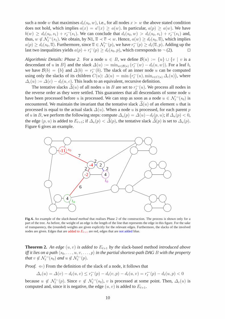
Algorithmic Details: Phase 2.For a nodeu ∈ B, we defineB(u) := {u} ∪ {v | v is adescendant ofu in B} and theslack∆(u) := minw∈B(u) (r←ℓ (w)− dℓ(u, w)). For a leafb,we haveB(b) = {b} and∆(b) = r←ℓ (b). The slack of an inner nodeu can be computedusing only the slacks of its childrenC(u): ∆(u) = min

(r←ℓ (u), minc∈C(u) ∆c(u)

), where

∆c(u) := ∆(c)− dℓ(u, c). This leads to an equivalent, recursive definition.The tentative slacks∆(u) of all nodesu in B are set tor←ℓ (u). We process all nodes in

the reverse order as they were settled. This guarantees thatall descendants of some nodeuhave been processed beforeu is processed. We can stop as soon as a nodeu ∈ N→ℓ (s0) isencountered. We maintain the invariant that the tentative slack ∆(u) of an elementu that isprocessed is equal to the actual slack∆(u). When a nodeu is processed, for each parentpof u in B, we perform the following steps: compute∆u(p) = ∆(u)−dℓ(p, u); if ∆u(p) < 0,the edge(p, u) is added toEℓ+1; if ∆u(p) < ∆(p), the tentative slack∆(p) is set to∆u(p).Figure 6 gives an example.

.

-11.

4

-4

.

p

18

1716

22

19

23

20 21

14

13

15

2524

2

-2

67

.

.

4

7

2

2

6

2

t0

t0

s0

Fig. 6. An example of theslack-based methodthat realises Phase 2 of the construction. The process is shown only for apart of the tree. As before, the weight of an edge is the lengthof the line that represents the edge in this figure. For the sakeof transparency, the (rounded) weights are given explicitly for the relevant edges. Furthermore, the slacks of the involvednodes are given. Edges that areadded toEℓ+1 are red, edges that arenot addedblue.

Theorem 2. An edge(u, v) is added toEℓ+1 by theslack-based methodintroduced aboveiff it lies on a path〈s0, . . . , u, v, . . . , p〉 in the partial shortest-path DAGB with the propertythatv 6∈ N→ℓ (s0) andu 6∈ N←ℓ (p).

Proof. ⇐) From the definition of the slack of a node, it follows that

∆v(u) = ∆(v)− dℓ(u, v) ≤ r←ℓ (p)− dℓ(v, p)− dℓ(u, v) = r←ℓ (p)− dℓ(u, p) < 0

becauseu 6∈ N←ℓ (p). Sincev 6∈ N→ℓ (s0), v is processed at some point. Then,∆v(u) iscomputed and, since it is negative, the edge(u, v) is added toEℓ+1.

10

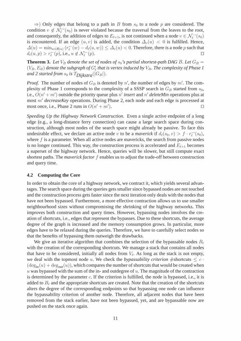
⇒) Only edges that belong to a path inB from s0 to a nodep are considered. Theconditionv 6∈ N→ℓ (s0) is never violated because the traversal from the leaves to the root,and consequently, the addition of edges toEℓ+1, is not continued when a nodev ∈ N→ℓ (s0)is encountered. If an edge(u, v) is added, the condition∆v(u) < 0 is fulfilled. Hence,∆(u) = minw∈B(u) (r←ℓ (w)− dℓ(u, w)) ≤ ∆v(u) < 0. Therefore, there is a nodep such thatdℓ(u, p) > r←ℓ (p), i.e.,u 6∈ N←ℓ (p). ⊓⊔Theorem 3. LetVB denote the set of nodes ofs0’s partial shortest-path DAGB. LetGB =(VB, EB) denote the subgraph ofG′ℓ that is vertex induced byVB. The complexity of Phase 1and 2 started froms0 is TDijkstra(|GB|).Proof. The number of nodes ofGB is denoted byn′, the number of edges bym′. The com-plexity of Phase 1 corresponds to the complexity of a SSSP search in GB started froms0,i.e.,O(n′ + m′) outside the priority queue plusn′ insertandn′ deleteMinoperations plus atmostm′ decreaseKeyoperations. During Phase 2, each node and each edge is processed atmost once, i.e., Phase 2 runs inO(n′ + m′). ⊓⊔

Speeding Up the Highway Network Construction.Even a single active endpoint of a longedge (e.g., a long-distance ferry connection) can cause a large search space during con-struction, although most nodes of the search space might already be passive. To face thisundesirable effect, we declare an active nodev to be amaverickif dℓ(s0, v) > f · r→ℓ (s0),wheref is a parameter. When all active nodes are mavericks, the search from passive nodesis no longer continued. This way, the construction process is accelerated andEℓ+1 becomesa superset of the highway network. Hence, queries will be slower, but still compute exactshortest paths. Themaverick factorf enables us to adjust the trade-off between constructionand query time.

4.2 Computing the Core

In order to obtain the core of a highway network, we contract it, which yields several advan-tages. The search space during the queries gets smaller since bypassed nodes are not touchedand the construction process gets faster since the next iteration only deals with the nodes thathave not been bypassed. Furthermore, a more effective contraction allows us to use smallerneighbourhood sizes without compromising the shrinking ofthe highway networks. Thisimproves both construction and query times. However, bypassing nodes involves the cre-ation of shortcuts, i.e., edges that represent the bypasses. Due to these shortcuts, the averagedegree of the graph is increased and the memory consumption grows. In particular, moreedges have to be relaxed during the queries. Therefore, we have to carefully select nodes sothat the benefits of bypassing them outweigh the drawbacks.

We give an iterative algorithm that combines the selection of the bypassable nodesBℓ

with the creation of the corresponding shortcuts. We managea stack that contains all nodesthat have to be considered, initially all nodes fromVℓ. As long as the stack is not empty,we deal with the topmost nodeu. We check thebypassability criterion#shortcuts≤ c ·(degin(u) + degout(u)), which compares the number of shortcuts that would be created whenu was bypassed with the sum of the in- and outdegree ofu. The magnitude of the contractionis determined by the parameterc. If the criterion is fulfilled, the node is bypassed, i.e., itisadded toBℓ and the appropriate shortcuts are created. Note that the creation of the shortcutsalters the degree of the corresponding endpoints so that bypassing one node can influencethe bypassability criterion of another node. Therefore, all adjacent nodes that have beenremoved from the stack earlier, have not been bypassed, yet,and are bypassable now arepushed on the stack once again.

11

Theorem 4. If c < 2, |E ′ℓ| is in O(|Vℓ|+ |Eℓ|).Proof. If a nodeu is bypassed, the number of edges in the (tentative) core is increased byDu := #shortcuts−degin(u)−degout(u). (We have to subtractdegin(u) anddegout(u) sincethe edges incident tou no longer belong to the core.) Note that#shortcuts= degin(u) ·degout(u)− deg↔(u), wheredeg↔(u) denotes the number of adjacent nodesv that are con-nected tou by both an edge(u, v) and an edge(v, u). (We have to subtractdeg↔(u) to ac-count for the fact that a ‘shortcut’ that would be a self-loopis not created.) We can concludethatDu ≤ degin(u) · degout(u) − degin(u)− degout(u). If degin(u) ≤ 1 or degout(u) ≤ 1,we obtainDu ≤ 0. Now, we deal with the case thatdegin(u) ≥ 2 anddegout(u) ≥ 2.Sincedeg↔(u) ≤ min(degin(u), degout(u)), a node that fulfils the bypassability criterionalso fulfilsdegin(u) · degout(u) ≤ c · (degin(u) + degout(u)) + min(degin(u), degout(u)).The inequalityx · y ≤ c(x + y) + min(x, y) has only finitely many solutions(x, y) forx, y ∈ N, x, y ≥ 2 if c ∈ R is a constant less than 2. Consider the solution(x, y) that max-imisesk := x · y. If there is no solution, takek := 0. Note thatk is a constant that onlydepends on the constantc. We can conclude thatDu ≤ k.

Each node fromVℓ is bypassed at most once. For each bypassed node, the number ofedges in the (tentative) core is increased by at mostk. Therefore,|E ′ℓ| ≤ k · |Vℓ|+ |Eℓ|. ⊓⊔

If we used#shortcuts≤ max (degin(u), degout(u)) as bypassability criterion, we wouldget a contraction that would be very similar to our earlier trees-and-lines method [23]. Notethat the general version presented above allows a more effective contraction by settingcappropriately.

Limiting Component Sizes.To reduce the observed maximum query time, we implementa limit on the number of hops a shortcut may represent. By thismeans, the sizes of thecomponents of bypassed nodes are reduced—in particular, the first contraction step tendedto create quite large components of bypassed nodes so that ittook a long time to leave sucha component when the search was started from within it.

5 Query

Our highway query algorithmis a modification of the bidirectional version of Dijkstra’salgorithm. Note that in contrast to the construction, during the query we neednot to keeptrack of ambiguous shortest paths. For now, we assume that the search isnot aborted whenboth search scopes meet. This matter is dealt with in Section5.3. We only describe themodifications of the forward search since forward and backward search are symmetric. Inaddition to thedistancefrom the source, each node is associated with the searchlevelandthegap to the ‘next applicable neighbourhood border’. The search starts at the source nodes in level 0. First, a local search in the neighbourhood ofs is performed, i.e., the gap to thenext border is set to the neighbourhood radius ofs in level 0. When a nodev is settled, itadopts the gap of its parentu minus the length of the edge(u, v). As long as we stay insidethe current neighbourhood, everything works as usual. However, if an edge(u, v) crossesthe neighbourhood border (i.e., the length of the edge is greater than the gap), we switchto a higher search levelℓ. The nodeu becomes anentrance pointto the higher level. If thelevel of the edge(u, v) is less than the new search levelℓ, the edge isnot relaxed—thisis one of the two restrictions that cause the speedup in comparison to Dijkstra’s algorithm(Restriction 1). Otherwise, the edge is relaxed:v adopts the new search levelℓ and the gapto the border of the neighbourhood ofu in levelℓ sinceu is the corresponding entrance pointto levelℓ.

12

We have to deal with the special case that an entrance point tolevel ℓ does not belongto the core of levelℓ. In this case, the search is continued inside a component of bypassednodes till the level-ℓ core is entered, i.e., a nodeu ∈ V ′ℓ is settled. At this point,u is assignedthe gap to the border of the level-ℓ neighbourhood ofu. Note that before the core is entered(i.e., inside a component of bypassed nodes), the gap has been infinity (according to R1). Toincrease the speedup, we introduce another restriction (Restriction 2): when a nodeu ∈ V ′ℓ issettled, all edges(u, v) that lead to a bypassed nodev ∈ Bℓ in search levelℓ arenot relaxed,i.e., once entered the core, we will never leave it again.

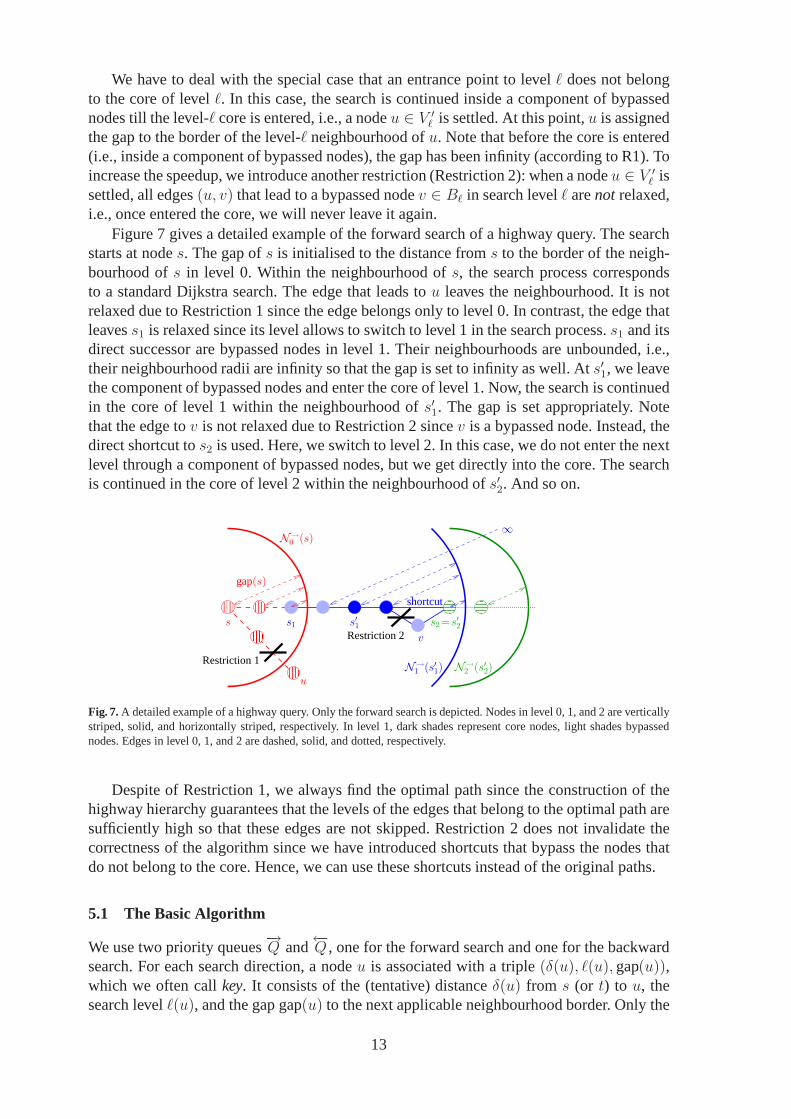
Figure 7 gives a detailed example of the forward search of a highway query. The searchstarts at nodes. The gap ofs is initialised to the distance froms to the border of the neigh-bourhood ofs in level 0. Within the neighbourhood ofs, the search process correspondsto a standard Dijkstra search. The edge that leads tou leaves the neighbourhood. It is notrelaxed due to Restriction 1 since the edge belongs only to level 0. In contrast, the edge thatleavess1 is relaxed since its level allows to switch to level 1 in the search process.s1 and itsdirect successor are bypassed nodes in level 1. Their neighbourhoods are unbounded, i.e.,their neighbourhood radii are infinity so that the gap is set to infinity as well. Ats′1, we leavethe component of bypassed nodes and enter the core of level 1.Now, the search is continuedin the core of level 1 within the neighbourhood ofs′1. The gap is set appropriately. Notethat the edge tov is not relaxed due to Restriction 2 sincev is a bypassed node. Instead, thedirect shortcut tos2 is used. Here, we switch to level 2. In this case, we do not enter the nextlevel through a component of bypassed nodes, but we get directly into the core. The searchis continued in the core of level 2 within the neighbourhood of s′2. And so on.

������������

������������

������

������

������

������

������������

������������

N→0

(s)

N→1

(s′1)

s s1 s′1

gap(s)

∞

Restriction 1 N→2

(s′2)

s2 =s′2

u

v

shortcut

Restriction 2

Fig. 7.A detailed example of a highway query. Only the forward search is depicted. Nodes in level 0, 1, and 2 are verticallystriped, solid, and horizontally striped, respectively. In level 1, dark shades represent core nodes, light shades bypassednodes. Edges in level 0, 1, and 2 are dashed, solid, and dotted, respectively.

Despite of Restriction 1, we always find the optimal path since the construction of thehighway hierarchy guarantees that the levels of the edges that belong to the optimal path aresufficiently high so that these edges are not skipped. Restriction 2 does not invalidate thecorrectness of the algorithm since we have introduced shortcuts that bypass the nodes thatdo not belong to the core. Hence, we can use these shortcuts instead of the original paths.

5.1 The Basic Algorithm

We use two priority queues−→Q and

←−Q , one for the forward search and one for the backward

search. For each search direction, a nodeu is associated with a triple(δ(u), ℓ(u), gap(u)),which we often callkey. It consists of the (tentative) distanceδ(u) from s (or t) to u, thesearch levelℓ(u), and the gap gap(u) to the next applicable neighbourhood border. Only the

13

first componentδ(u) is used to decide the priority within the queue.2 We use the remainingtwo components for a tie breaking rule in the case that the same node is reached with twodifferent keysk := (δ, ℓ, gap) andk′ := (δ′, ℓ′, gap′) such thatδ = δ′. Then, we preferk tok′ iff ℓ > ℓ′ or ℓ = ℓ′∧gap< gap′. Note thatanyother tie breaking rule (or even omitting anexplicit rule) will yield a correct algorithm. However, thechosen rule is most aggressive andhas a positive effect on the performance. Figure 8 contains the pseudo-code of the highwayquery algorithm.

input: source nodes and target nodetoutput: distanced(s, t)

1 d′ :=∞;2 insert(

−→Q, s, (0, 0, r→0 (s))); insert(

←−Q, t, (0, 0, r←0 (t)));

3 while (−→Q ∪

←−Q 6= ∅) do {

4 select direction⇌ ∈ {→,←} such that⇌

Q 6= ∅;

5 u := deleteMin(⇌

Q);6 if u has been settled from both directionsthen d′ := min(d′,

−→δ (u) +

←−δ (u));

7 if gap(u) 6=∞ then gap′ := gap(u) elsegap′ := r⇌

ℓ(u)(u);

8 foreach e = (u, v) ∈⇌

E do {9 for (ℓ := ℓ(u), gap:= gap′; w(e) > gap;

ℓ++, gap:= r⇌

ℓ (u)); // go “upwards”10 if ℓ(e) < ℓ then continue; // Restriction 1

11 if u ∈ V ′ℓ ∧ v ∈ Bℓ then continue; // Restriction 2

12 k := (δ(u) + w(e), ℓ, gap− w(e));

13 if v has been reachedthen decreaseKey(⇌

Q, v, k); elseinsert(⇌

Q, v, k);14 }15 }16 return d′;

Fig. 8.The highway query algorithm. Differences to the bidirectional version of Dijkstra’s algorithm are marked: additionaland modified lines have a framed line number; in modified lines, the modifications are underlined.

Remarks:

– Line 4: The correctness of the algorithm does not depend on the strategy that determinesthe order in which the forward and the backward searches are processed. However, thechoice of the strategy can affect the running time in the casethat an abort-on-successcriterion is applied (see Section 5.3).

– Line 7: This line deals with the special case that the entrance point did not belong to thecore when the current search levelℓ was entered, i.e., the gap was set to infinity. In thiscase, the gap is set tor⇌

ℓ(u)(u). This is correct even ifu does not belong to the core, either,because in this case the gap stays at infinity.

– Line 9: It might be necessary to go upwards more than one levelin a single step.– Line 13: In the decreaseKey operation, the old key ofv is only replaced byk if the above

mentioned condition is fulfilled, i.e., if (a) the tentativedistance is improved or (b) staysunchanged while the tie breaking rule succeeds. In the latter case (b), no priority queueoperation is invoked since the priority (the tentative distance) has not changed.3

2 If the search direction is not clear from the context, we willexplicitly write−→δ (u) and

←−δ (u) to distinguish betweenu’s

priority in−→Q and

←−Q .

3 That way, we also avoid problems that otherwise could arise when an already settled node is reached once again via azero weight edge.

14

Algorithmic Details. If we group the outgoing edges(u, v) of each nodeu by level, wecan avoid looking at edges(u, v) in levelsℓ(u, v) < ℓ(u) since Restriction 1 would alwaysapply to them. We can do without explicitly testing Restriction 2 if all edges(u, v) withk := ℓ(u, v), u ∈ V ′k , andv ∈ Bk have been downgraded to levelk − 1. Then, the test ofRestriction 1 also covers Restriction 2.

5.2 Proof of Correctness

Difficulties. Although the basic concepts (e.g. the definition of the highway network) andthe algorithm are quite simple, the proof of correctness gets surprisingly complicated. Themain reason for that is the fact that we cannot prove thattheshortest path is found since theremight be several shortest paths of the same length. We could assume that the shortest pathsin the input are unique or that the uniqueness can be guaranteed by adding small fractionsto the edge weights as it is done by other authors who face similar problems. However, theformer would be too restrictive since usually, in real-world road networks, there are at leasta few ambiguous instances, and a reliable realisation of thelatter would be rather difficult.Furthermore, the introduction of shortcuts adds a lot of ambiguity even if it was not presentin the input.

Therefore, if we pick any shortest pathP to show that it is found by the query algorithm,it can happen that a nodeu on P is settled from another node than its predecessor onP .Of course, in this case,u will still be assigned the optimal distance from the source,butthe search level and the distance to the next neighbourhood border may be different thanexpected so that we have to adapt to the new situation.

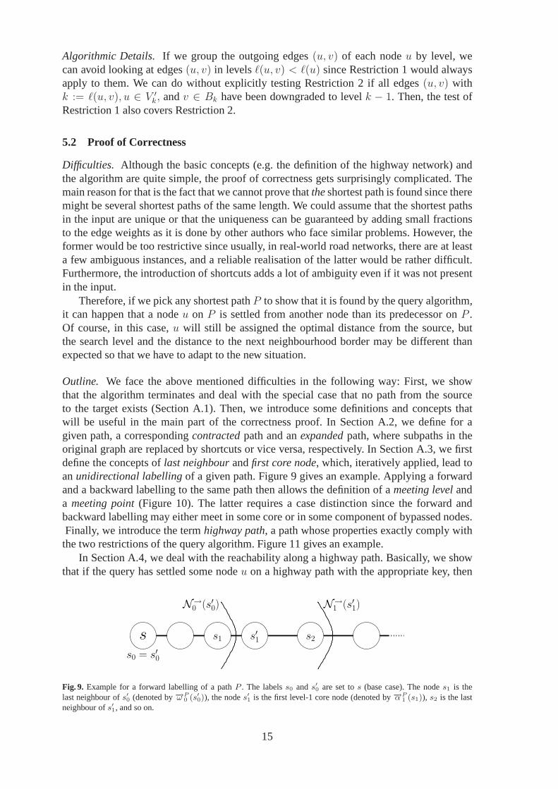
Outline. We face the above mentioned difficulties in the following way: First, we showthat the algorithm terminates and deal with the special casethat no path from the sourceto the target exists (Section A.1). Then, we introduce some definitions and concepts thatwill be useful in the main part of the correctness proof. In Section A.2, we define for agiven path, a correspondingcontractedpath and anexpandedpath, where subpaths in theoriginal graph are replaced by shortcuts or vice versa, respectively. In Section A.3, we firstdefine the concepts oflast neighbourandfirst core node, which, iteratively applied, lead toanunidirectional labellingof a given path. Figure 9 gives an example. Applying a forwardand a backward labelling to the same path then allows the definition of a meeting levelanda meeting point(Figure 10). The latter requires a case distinction since the forward andbackward labelling may either meet in some core or in some component of bypassed nodes.Finally, we introduce the termhighway path, a path whose properties exactly comply withthe two restrictions of the query algorithm. Figure 11 givesan example.

In Section A.4, we deal with the reachability along a highwaypath. Basically, we showthat if the query has settled some nodeu on a highway path with the appropriate key, then

s1 s′1 s2

N→1 (s′1)

s0 = s′0

N→0 (s′0)

s

Fig. 9. Example for a forward labelling of a pathP . The labelss0 ands′0 are set tos (base case). The nodes1 is thelast neighbour ofs′0 (denoted by−→ω P

0 (s′0)), the nodes′1 is the first level-1 core node (denoted by−→α P

1 (s1)), s2 is the lastneighbour ofs′1, and so on.

15

s0=s′0 s1 s′1

t′2t3

s′2

t′0=t0t′1=t1

p

s2

t2

s t

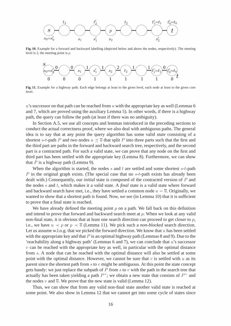
Fig. 10.Example for a forward and backward labelling (depicted below and above the nodes, respectively). The meetinglevel is 2, the meeting point isp.

s1 s′1s0=s′0

0 1

ss2

1

t2 t′0=t0t′1=t1t00 011 1

00 1 1 2 1 1 0

Fig. 11. Example for a highway path. Each edge belongs at least to the given level, each node at least to the given corelevel.

u’s successor on that path can be reached fromu with the appropriate key as well (Lemmas 6and 7, which are proved using the auxiliary Lemma 5). In otherwords, if there is a highwaypath, the query can follow the path (at least if there was no ambiguity).

In Section A.5, we use all concepts and lemmas introduced in the preceding sections toconduct the actual correctness proof, where we also deal with ambiguous paths. The generalidea is to say that at any point the query algorithm has some valid stateconsisting of ashortests-t-pathP and two nodesu � u that splitP into three parts such that the first andthe third part are paths in the forward and backward search tree, respectively, and the secondpart is a contracted path. For such a valid state, we can provethat any node on the first andthird part has been settled with the appropriate key (Lemma 8). Furthermore, we can showthatP is a highway path (Lemma 9).

When the algorithm is started, the nodess andt are settled and some shortests-t-pathP in the original graph exists. (The special case that nos-t-path exists has already beendealt with.) Consequently, ourinitial state is composed of the contracted version ofP andthe nodess andt, which makes it a valid state. Afinal state is a valid state where forwardand backward search have met, i.e., they have settled a common nodeu = u. Originally, wewanted to show that a shortest path is found. Now, we see (in Lemma 10) that it is sufficientto prove that a final state is reached.

We have already defined the meeting pointp on a path. We fall back on this definitionand intend to prove that forward and backward search meet atp. When we look at any validnon-final state, it is obvious that at least one search direction can proceed to get closer top,i.e., we haveu ≺ p or p ≺ u (Lemma 11). We pick such anon-blockedsearch direction.Let us assume w.l.o.g. that we picked the forward direction.We know thatu has been settledwith the appropriate key and thatP is an optimal highway path (Lemmas 8 and 9). Due to the‘reachability along a highway path’ (Lemmas 6 and 7), we can conclude thatu’s successorv can be reached with the appropriate key as well, in particular with the optimal distancefrom s. A node that can be reached with the optimal distance will also be settled at somepoint with the optimal distance. However, we cannot be sure thatv is settled withu as itsparent since the shortest path froms to v might be ambiguous. At this point the state conceptgets handy: we just replace the subpath ofP from s to v with the path in the search tree thatactually has been taken yielding a pathP+; we obtain a new state that consists ofP + andthe nodesv andu. We prove that the new state is valid (Lemma 12).

Thus, we can show that from any valid non-final state another valid state is reached atsome point. We also show in Lemma 12 that we cannot get into some cycle of states since

16

in each step the length of the middle part of the path is decreased. Hence, starting from theinitial state, eventually a final state is reached so that a shortest path is found (Theorem 5).

The actual proof can be found in Appendix A.

5.3 Optimisations

Rearranging Nodes.Similar to [20], after the construction has been completed,we rearrangethe nodes by core level, which improves locality for the search in higher levels and, thus,reduces the number of cache misses.

Speeding Up the Search in the Topmost Level.Let us assume that we have a distance tablethat contains for any node pairs, t ∈ V ′L the optimal distancedL(s, t). Such a table canbe precomputed during the preprocessing phase by|V ′L| SSSP searches inG′L. Using thedistance table, we do not have to search in levelL. Instead, when we arrive at a nodeu ∈ V ′Lthat leads to levelL, we addu to the initially empty set

−→I or

←−I depending on the search

direction; we do not relax the edge that leads to levelL. After all entrance points have beenencountered, we consider all pairs(u, v) ∈ −→I ×←−I and compute the minimum path lengthD :=

−→δ (u) + dL(u, v) +

←−δ (v). Then, the length of the shortests-t-path is the minimum of

D and the lengthd′ of the tentative shortest path found so far (in case that the search scopeshave already met in a level< L).

For the sake of a simple incorporation of this optimisation into the highway query algo-rithm, we slightly revise the properties R1 and R2: we use twodistinguishable values∞1

and∞2 that are larger than any real number and setr⇌

ℓ (u) := ∞1 for any ℓ and any nodeu 6∈ V ′ℓ (R1) andr⇌

L (u) := ∞2 for any nodeu ∈ V ′L (R2). Then, we just add two lines toFigure 8 and modify Line 16:

between Lines 7 and 8:7a if gap′ 6=∞1 ∧ ℓ(u) = L then {

⇌

I :=⇌

I ∪{u}; continue;}between Lines 11 and 12:11a if gap 6=∞1 ∧ ℓ = L ∧ ℓ > ℓ(u) then {

⇌

I :=⇌

I ∪{u}; continue;}16 return min({d′} ∪ {−→δ (u) + dL(u, v) +

←−δ (v) | u ∈ −→I , v ∈ ←−I });

In Section A.6, we show that our proof of correctness still holds when the distance tableoptimisation is applied.

Abort on Success.In the bidirectional version of Dijkstra’s algorithm, we can abort thesearch as soon as both search scopes meet. Unfortunately, this would be incorrect for ourhighway query algorithm. Therefore, we use a more conservative criterion: after a tentativeshortest pathP ′ has been encountered (i.e., after both search scopes have met), the forward(backward) search is not continued if the minimum elementu of the forward (backward)queue has a keyδ(u) ≥ w(P ′). Obviously, the correctness of the algorithm is not invalidatedby this abort criterion. In [23] we tried using more sophisticated criteria in order to reducethe search space. However, it turned out that this simple criterion, since it can be evaluatedso efficiently, yields better query times in spite of a somewhat larger search space. Note thatwhen the distance table optimisation is used and random queries are performed, our simpleabort criterion is very close to an optimal criterion even with respect to the search spacesize: our experiments indicate that less than 1% of the search space is visited after the firstmeeting of forward and backward search.

17

5.4 Outputting Complete Path Descriptions

The highway query algorithm in Figure 8 only computes the distance froms to t. In orderto determine the actual shortest path, we need to store pointers from each node to its parentin the search tree. Note that the algorithm could be easily modified to computeall shortestpaths betweens andt by just storing more than one parent pointer in case of ambiguities.However, subsequently, we only deal with a single shortest path.

We face two problems in order to determine a complete description of the shortest path:(a) we have to bridge the gap between the forward and backwardtopmost core entrancepoints (in case that the distance table optimisation is used) and (b) we have to expand theused shortcuts to obtain the corresponding subpaths in the original graph.

Problem (a) can be solved using a simple algorithm: We start with the forward coreentrance pointu. As long as the backward entrance pointv has not been reached, we considerall outgoing edges(u, w) in the topmost core and check whetherdL(u, w) + dL(w, v) =dL(u, v); we pick an edge(u, w) that fulfils the equation, and we setu := w. The check canbe performed using the distance table. It allows us to greedily determine the next hop thatleads to the backward entrance point.

Problem (b) can be solved without using any extra data (Variant 1). For each shortcut(u, v) ∈ Sℓ on the shortest path, we perform a search fromu to v in order to determine therepresented path inGℓ. This search can be accelerated by using the knowledge that the firstedge of the path enters a componentC of bypassed nodes, the last edge leads tov, and allother edges are situated within the componentC. The represented path inGℓ may containshortcuts from setsSk, k < ℓ, which are expanded recursively. In the end, we obtain therepresented path fromu to v in the original graph.

However, if a fast output routine is required, it is necessary to spend some additionalspace to accelerate the unpacking process. We use a rather sophisticated data structure torepresent unpacking information for the shortcuts in a space-efficient way (Variant 2). Inparticular, we do not store a sequence of node IDs that describe a path that corresponds toa shortcut, but we store onlyhop indices: for each edge(u, v) on the path that should berepresented, we store its rank within the ordered group of edges that leaveu. Since in mostcases the degree of a node is very small, these hop indices canbe stored using only a fewbits. The unpacked shortcuts are stored in a recursive way, e.g., the description of a level-2shortcut may contain several level-1 shortcuts. Accordingly, the unpacking procedure worksrecursively.

To obtain a further speed-up, we have a variant of the unpacking data structures (Vari-ant 3) that caches the complete descriptions—without recursions—of all shortcuts that be-long to the topmost level, i.e., for these important shortcuts that are frequently used, we donot have to use a recursive unpacking procedure, but we can just append the correspondingsubpath to the resulting path.

5.5 Turning Restrictions

A turning restriction (in its simplest and most common form)is expressed as an edge pair((u, v), (v, w)): the edge(v, w) must not be traversed if the nodev has been reached via theedge(u, v). Dealing with turning restrictions is a well-studied problem [33, 34]. In principle,there are two basic approaches: modifying the query algorithm or modelling the restrictionsinto the graph, which introduces additional artificial nodes and edges at affected road junc-tions. The latter technique can be applied irrespective of the used query algorithm.

In case of highway hierarchies, we expect that modelling turning restrictions into thegraph only slightly deteriorates the performance since theartificial nodes usually have a

18

very small degree so that most of them get bypassed in the veryfirst contraction step. Fur-thermore, turning restrictions are often encountered at local streets that are not promoted tohigh levels of the hierarchy so that the negative impact is bounded to the lower levels. Withrespect to memory consumption, it is important to note that after the preprocessing has beencompleted, artificial nodes and edges at road junctions thatonly belong to level 0 can beabandoned provided that the query algorithm (which in level0 just corresponds to Dijkstra’salgorithm) is modified appropriately to handle turning restrictions.

6 Experiments

Apart from Section 6.8, all experimental results refer to the scenario where we only wantto compute the shortest-path length between two nodes without outputting the actual route.Turning restrictions are exclusively handled in Section 6.9.

6.1 Implementation

We implemented highway hierarchies in C++, using the C++ Standard Template Libraryand making extensive use ofgeneric programmingtechniques using C++’s template classmechanism. As graph data structure, we use our own implementation of anadjacency arrayextended by an additional layer that contains level-specific data for each node and level thatthe node belongs to. We use 32 bits to store edge weights and path lengths.Binary heapsare used as priority queues. Note that in case of road networks only a comparatively smallnumber ofdecreaseKey-operations is performed. Furthermore, the number of nodesthat arein the priority queue at the same time is very small in case of highway hierarchies (usuallyless than 100 nodes). Therefore, using a more sophisticatedpriority queue implementationis not likely to increase the performance significantly. Forsome more details on the imple-mentation, we refer to Appendix B.

6.2 Environment and Instances

The experiments were done on one core of a single AMD Opteron Processor 270 clocked at2.0 GHz with 8 GB main memory and 2× 1 MB L2 cache, running SuSE Linux 10.0 (kernel2.6.13). The program was compiled by the GNU C++ compiler 4.0.2 using optimisationlevel 3.

We deal with the road networks of Western Europe4 and of the USA (without Hawaii)and Canada. Both networks have been made available for scientific use by the companyPTV AG. The original graphs contain for each edge a length anda road category, e.g.,motorway, national road, regional road, urban street. We assign average speeds to the roadcategories5, compute for each edge the average travel time, and use it as weight. In addition,we perform experiments on a publicly available version of the US road network (withoutAlaska and Hawaii) that was obtained from the TIGER/Line Files [35]. However, in contrastto the PTV data, the TIGER graph is undirected, planarised and distinguishes only betweenfour road categories (40, 60, 80, 100 km/h), in fact 91% of allroads belong to the slowestcategory so that you cannot discriminate them.

Table 1 summarises important properties of the used road networks and the key resultsof the experiments.

4 Austria, Belgium, Denmark, France, Germany, Italy, Luxembourg, the Netherlands, Norway, Portugal, Spain, Sweden,Switzerland, and the UK

5 For Europe: 10, 20,. . ., 130 km/h; for USA/CAN: 16, 24, 32, 40, 56, 64, 72, 80, 88, 96, 96, 104, 112 km/h.

19

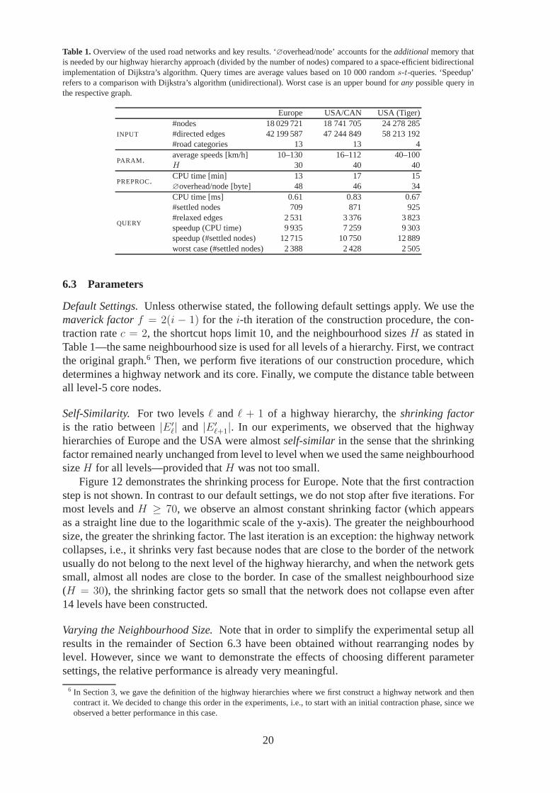
Table 1.Overview of the used road networks and key results. ‘∅overhead/node’ accounts for theadditionalmemory thatis needed by our highway hierarchy approach (divided by the number of nodes) compared to a space-efficient bidirectionalimplementation of Dijkstra’s algorithm. Query times are average values based on 10 000 randoms-t-queries. ‘Speedup’refers to a comparison with Dijkstra’s algorithm (unidirectional). Worst case is an upper bound foranypossible query inthe respective graph.

Europe USA/CAN USA (Tiger)

INPUT

#nodes 18 029 721 18 741 705 24 278 285#directed edges 42 199 587 47 244 849 58 213 192#road categories 13 13 4

PARAM.average speeds [km/h] 10–130 16–112 40–100H 30 40 40

PREPROC.CPU time [min] 13 17 15∅overhead/node [byte] 48 46 34

QUERY

CPU time [ms] 0.61 0.83 0.67#settled nodes 709 871 925#relaxed edges 2 531 3 376 3 823speedup (CPU time) 9 935 7 259 9 303speedup (#settled nodes) 12 715 10 750 12 889worst case (#settled nodes) 2 388 2 428 2 505

6.3 Parameters

Default Settings.Unless otherwise stated, the following default settings apply. We use themaverick factorf = 2(i − 1) for the i-th iteration of the construction procedure, the con-traction ratec = 2, the shortcut hops limit 10, and the neighbourhood sizesH as stated inTable 1—the same neighbourhood size is used for all levels ofa hierarchy. First, we contractthe original graph.6 Then, we perform five iterations of our construction procedure, whichdetermines a highway network and its core. Finally, we compute the distance table betweenall level-5 core nodes.

Self-Similarity. For two levelsℓ and ℓ + 1 of a highway hierarchy, theshrinking factoris the ratio between|E ′ℓ| and |E ′ℓ+1|. In our experiments, we observed that the highwayhierarchies of Europe and the USA were almostself-similarin the sense that the shrinkingfactor remained nearly unchanged from level to level when weused the same neighbourhoodsizeH for all levels—provided thatH was not too small.

Figure 12 demonstrates the shrinking process for Europe. Note that the first contractionstep is not shown. In contrast to our default settings, we do not stop after five iterations. Formost levels andH ≥ 70, we observe an almost constant shrinking factor (which appearsas a straight line due to the logarithmic scale of the y-axis). The greater the neighbourhoodsize, the greater the shrinking factor. The last iteration is an exception: the highway networkcollapses, i.e., it shrinks very fast because nodes that areclose to the border of the networkusually do not belong to the next level of the highway hierarchy, and when the network getssmall, almost all nodes are close to the border. In case of thesmallest neighbourhood size(H = 30), the shrinking factor gets so small that the network does not collapse even after14 levels have been constructed.

Varying the Neighbourhood Size.Note that in order to simplify the experimental setup allresults in the remainder of Section 6.3 have been obtained without rearranging nodes bylevel. However, since we want to demonstrate the effects of choosing different parametersettings, the relative performance is already very meaningful.

6 In Section 3, we gave the definition of the highway hierarchies where we first construct a highway network and thencontract it. We decided to change this order in the experiments, i.e., to start with an initial contraction phase, since weobserved a better performance in this case.

20

107

106

105

104

1000

100

10

1 0 2 4 6 8 10 12 14

#edg

es

level

H = 30H = 50H = 70H = 90

Fig. 12.Shrinking of the highway networks of Europe. For different neighbourhood sizesH and for each levelℓ, we plot|E′ℓ |, i.e., the number of edges that belong to the core of levelℓ.

In one test series (Figure 13), we used all the default settings except for the neighbour-hood sizeH, which we varied in steps of 5. On the one hand, ifH is too small, the shrinkingof the highway networks is less effective so that the level-5core is still quite big. Hence, weneed much time and space to precompute and store the distancetable. On the other hand,if H gets bigger, the time needed to preprocess the lower levels increases because the areacovered by the local searches depends on the neighbourhood size. Furthermore, during aquery, it takes longer to leave the lower levels in order to get to the topmost level wherethe distance table can be used. Thus, the query time increases as well. We observe that thepreprocessing time is minimised for neighbourhood sizes around 40. In particular, the opti-mal neighbourhood size does not vary very much from graph to graph. In other words, if weused the same parameterH, say 40, for all road networks, the resulting performance wouldbe very close to the optimum. Obviously, choosing differentneighbourhood sizes leads todifferent space-time trade-offs.

10

12

14

16

18

20

22

20 30 40 50 60 70 80 90

Pre

proc

essi

ng T

ime

[min

]

20

30

40

50

60

70

80

90

20 30 40 50 60 70 80 90

Mem

ory

Ove

rhea

d pe

r N

ode

[byt

e]

EuropeUSA/CAN

USA

0.6 0.7 0.8 0.9

1 1.1 1.2 1.3 1.4 1.5 1.6 1.7

20 30 40 50 60 70 80 90

Que

ry T

ime

[ms]

Fig. 13.Preprocessing and query performance depending on the neighbourhood sizeH .

Varying the Contraction Rate.In another test series (Table 2a), we did not use a distance ta-ble, but repeated the construction process until the topmost level was empty or the hierarchyconsisted of 15 levels. We varied the contraction ratec from 0.5 to 2.5. In case ofc = 0.5(andH = 30), the shrinking of the highway networks does not work properly so that the top-most level is still very big. This yields huge query times. Choosing larger contraction rates

21

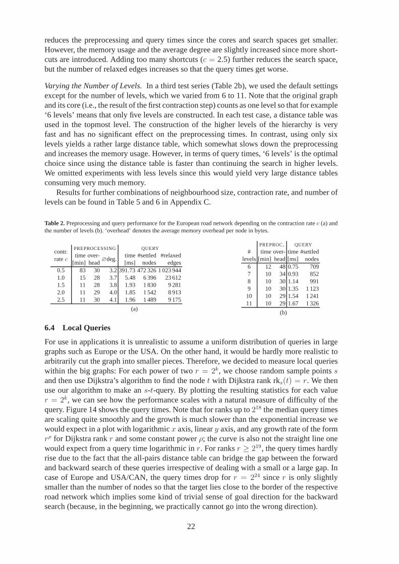
reduces the preprocessing and query times since the cores and search spaces get smaller.However, the memory usage and the average degree are slightly increased since more short-cuts are introduced. Adding too many shortcuts (c = 2.5) further reduces the search space,but the number of relaxed edges increases so that the query times get worse.

Varying the Number of Levels.In a third test series (Table 2b), we used the default settingsexcept for the number of levels, which we varied from 6 to 11. Note that the original graphand its core (i.e., the result of the first contraction step) counts as one level so that for example‘6 levels’ means that only five levels are constructed. In each test case, a distance table wasused in the topmost level. The construction of the higher levels of the hierarchy is veryfast and has no significant effect on the preprocessing times. In contrast, using only sixlevels yields a rather large distance table, which somewhatslows down the preprocessingand increases the memory usage. However, in terms of query times, ‘6 levels’ is the optimalchoice since using the distance table is faster than continuing the search in higher levels.We omitted experiments with less levels since this would yield very large distance tablesconsuming very much memory.

Results for further combinations of neighbourhood size, contraction rate, and number oflevels can be found in Table 5 and 6 in Appendix C.

Table 2.Preprocessing and query performance for the European road network depending on the contraction ratec (a) andthe number of levels (b). ‘overhead’ denotes the average memory overhead per node in bytes.

contr.PREPROCESSING QUERY

ratectime over-

∅deg.time #settled #relaxed

[min] head [ms] nodes edges0.5 83 30 3.2391.73 472 326 1 023 9441.0 15 28 3.7 5.48 6 396 23 6121.5 11 28 3.8 1.93 1 830 9 2812.0 11 29 4.0 1.85 1 542 8 9132.5 11 30 4.1 1.96 1 489 9 175

(a)

PREPROC. QUERY

# time over-time #settledlevels[min] head[ms] nodes

6 12 48 0.75 7097 10 34 0.93 8528 10 30 1.14 9919 10 30 1.35 1 12310 10 29 1.54 1 24111 10 29 1.67 1 326

(b)

6.4 Local Queries

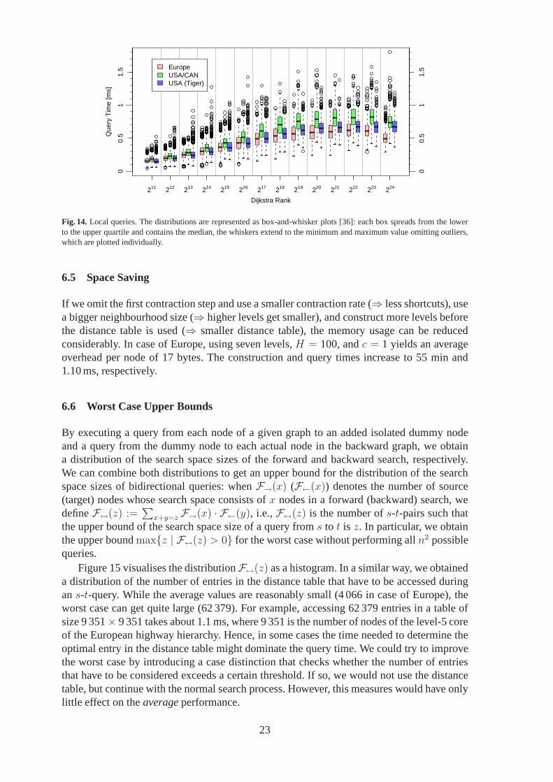
For use in applications it is unrealistic to assume a uniformdistribution of queries in largegraphs such as Europe or the USA. On the other hand, it would behardly more realistic toarbitrarily cut the graph into smaller pieces. Therefore, we decided to measure local querieswithin the big graphs: For each power of twor = 2k, we choose random sample pointssand then use Dijkstra’s algorithm to find the nodet with Dijkstra rank rks(t) = r. We thenuse our algorithm to make ans-t-query. By plotting the resulting statistics for each valuer = 2k, we can see how the performance scales with a natural measureof difficulty of thequery. Figure 14 shows the query times. Note that for ranks upto 218 the median query timesare scaling quite smoothly and the growth is much slower thanthe exponential increase wewould expect in a plot with logarithmicx axis, lineary axis, and any growth rate of the formrρ for Dijkstra rankr and some constant powerρ; the curve is also not the straight line onewould expect from a query time logarithmic inr. For ranksr ≥ 219, the query times hardlyrise due to the fact that the all-pairs distance table can bridge the gap between the forwardand backward search of these queries irrespective of dealing with a small or a large gap. Incase of Europe and USA/CAN, the query times drop forr = 224 sincer is only slightlysmaller than the number of nodes so that the target lies closeto the border of the respectiveroad network which implies some kind of trivial sense of goaldirection for the backwardsearch (because, in the beginning, we practically cannot gointo the wrong direction).

22

Dijkstra Rank

Que

ry T

ime

[ms]

211 212 213 214 215 216 217 218 219 220 221 222 223 224

01

0.5

1.5

01

0.5

1.5Europe

USA/CANUSA (Tiger)

Fig. 14.Local queries. The distributions are represented as box-and-whisker plots [36]: each box spreads from the lowerto the upper quartile and contains the median, the whiskers extend to the minimum and maximum value omitting outliers,which are plotted individually.

6.5 Space Saving

If we omit the first contraction step and use a smaller contraction rate (⇒ less shortcuts), usea bigger neighbourhood size (⇒ higher levels get smaller), and construct more levels beforethe distance table is used (⇒ smaller distance table), the memory usage can be reducedconsiderably. In case of Europe, using seven levels,H = 100, andc = 1 yields an averageoverhead per node of 17 bytes. The construction and query times increase to 55 min and1.10 ms, respectively.

6.6 Worst Case Upper Bounds

By executing a query from each node of a given graph to an addedisolated dummy nodeand a query from the dummy node to each actual node in the backward graph, we obtaina distribution of the search space sizes of the forward and backward search, respectively.We can combine both distributions to get an upper bound for the distribution of the searchspace sizes of bidirectional queries: whenF→(x) (F←(x)) denotes the number of source(target) nodes whose search space consists ofx nodes in a forward (backward) search, wedefineF↔(z) :=

∑x+y=z F→(x) · F←(y), i.e.,F↔(z) is the number ofs-t-pairs such that

the upper bound of the search space size of a query froms to t is z. In particular, we obtainthe upper boundmax{z | F↔(z) > 0} for the worst case without performing alln2 possiblequeries.

Figure 15 visualises the distributionF↔(z) as a histogram. In a similar way, we obtaineda distribution of the number of entries in the distance tablethat have to be accessed duringans-t-query. While the average values are reasonably small (4 066in case of Europe), theworst case can get quite large (62 379). For example, accessing 62 379 entries in a table ofsize 9 351× 9 351 takes about 1.1 ms, where 9 351 is the number of nodes of the level-5 coreof the European highway hierarchy. Hence, in some cases the time needed to determine theoptimal entry in the distance table might dominate the querytime. We could try to improvethe worst case by introducing a case distinction that checkswhether the number of entriesthat have to be considered exceeds a certain threshold. If so, we would not use the distancetable, but continue with the normal search process. However, this measures would have onlylittle effect on theaverageperformance.

23

1014

1012

1010

108

106

104

100

0 500 1000 1500 2000 2500

# s-

t-pa

irs

Search Space Size

EuropeUSA/CAN

USA (Tiger)

Fig. 15. Histogram of upper bounds for the search space sizes ofs-t-queries. To increase readability, only the outline ofthe histogram is plotted instead of the complete boxes.

6.7 Comparisons

In Table 3, we compare our highway hierarchies with some of the most competitive methodswhere experimental results are available for the Western European and the US road network,namely with the REAL algorithm [20], transit-node routing [27], and highway-node routing[29]. For REAL and transit-node routing slightly smaller graphs were used, namely thelargest connected component of each road network consisting of about 99% of all nodes.Experiments with the REAL algorithm have been performed on aslightly different machine(dual-processor, 2.4 GHz AMD Opteron).

Although a comparison is difficult since all approaches allow different choices of pa-rameter settings yielding different space-time trade-offs, we can make some general state-ments: The strength of transit-node routing is clearly the extremely good query performance.Highway-node routing has an outstandingly low memory consumption, while the querytimes are competitive to highway hierarchies and REAL or even slightly superior in caseof the US road network. Highway hierarchies can achieve verylow preprocessing timesor a quite low memory consumption, while query times are reasonably good in all cases.REAL’s performance is similar to highway hierarchies except for the preprocessing times,which tend to be considerably higher.

It is very important to note that both highway-node routing and the implementation oftransit-node routing considered in this section are based on our highway hierarchies. Thus,at the moment neither of these methods can supersede the highway hierarchies approach.Actually, the results for highway-node routing are better than the ones published in [29]

Table 3.Comparison between highway hierarchies (HH), the REAL algorithm, transit-node routing (TNR) and highway-node routing (HNR). For the former three approaches, different parameter settings are examined. ‘disk space’ denotes thetotal amount of memory needed to store the preprocessed dataincluding the original graph on disk.

Europe USA (Tiger)

methodPREPROCESSING QUERY PREPROCESSING QUERY

time disk space time #settledtime disk space time #settled[min] [MB] [ms] nodes [min] [MB] [ms] nodes

HH 13 1 241 0.61 709 15 1 324 0.67 925HH (mem) 55 697 1.10 1 863 70 942 1.21 2 143REAL (16,1) 97 1 849 1.22 814 64 3 028 1.14 675REAL (64,16) 141 1 0151.11 679 121 1 5751.05 540TNR (eco) 46 2 304 0.0134 N/A 59 3 073 0.0115 N/ATNR (gen) 164 4 7140.0056 N/A 205 6 1080.0049 N/AHNR 15 503 0.88 1 017 16 640 0.50 760

24

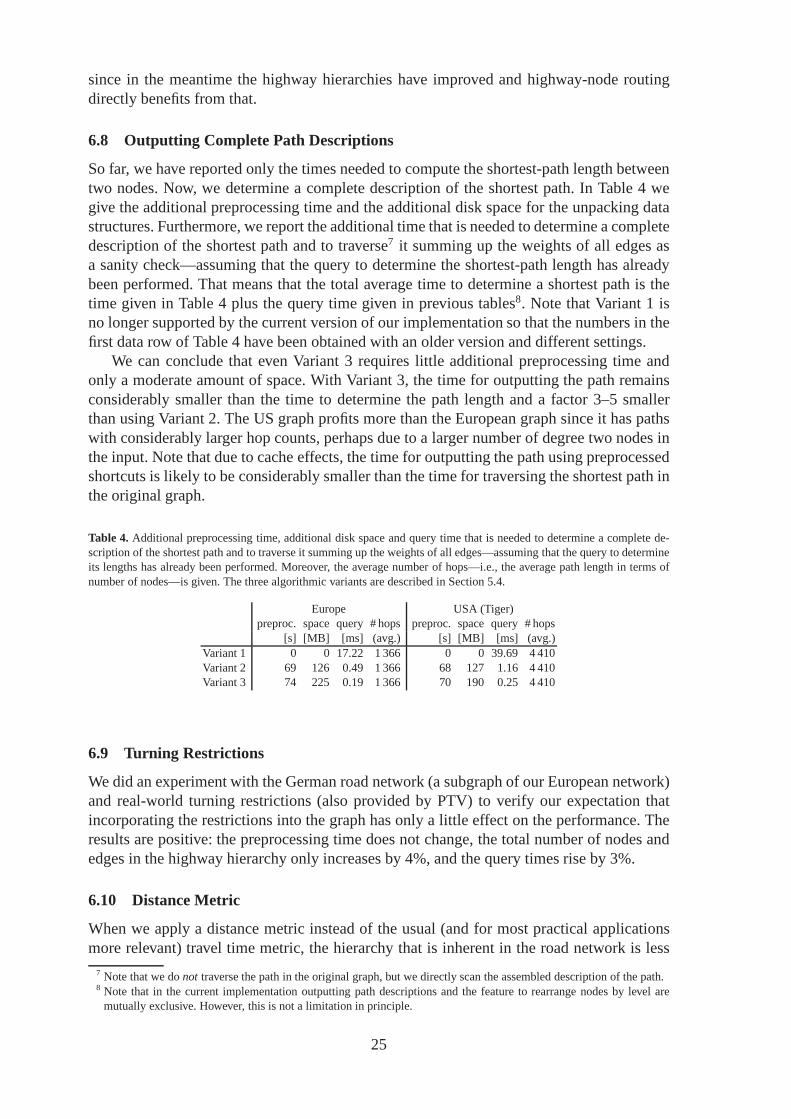
since in the meantime the highway hierarchies have improvedand highway-node routingdirectly benefits from that.

6.8 Outputting Complete Path Descriptions

So far, we have reported only the times needed to compute the shortest-path length betweentwo nodes. Now, we determine a complete description of the shortest path. In Table 4 wegive the additional preprocessing time and the additional disk space for the unpacking datastructures. Furthermore, we report the additional time that is needed to determine a completedescription of the shortest path and to traverse7 it summing up the weights of all edges asa sanity check—assuming that the query to determine the shortest-path length has alreadybeen performed. That means that the total average time to determine a shortest path is thetime given in Table 4 plus the query time given in previous tables8. Note that Variant 1 isno longer supported by the current version of our implementation so that the numbers in thefirst data row of Table 4 have been obtained with an older version and different settings.

We can conclude that even Variant 3 requires little additional preprocessing time andonly a moderate amount of space. With Variant 3, the time for outputting the path remainsconsiderably smaller than the time to determine the path length and a factor 3–5 smallerthan using Variant 2. The US graph profits more than the European graph since it has pathswith considerably larger hop counts, perhaps due to a largernumber of degree two nodes inthe input. Note that due to cache effects, the time for outputting the path using preprocessedshortcuts is likely to be considerably smaller than the timefor traversing the shortest path inthe original graph.

Table 4. Additional preprocessing time, additional disk space and query time that is needed to determine a complete de-scription of the shortest path and to traverse it summing up the weights of all edges—assuming that the query to determineits lengths has already been performed. Moreover, the average number of hops—i.e., the average path length in terms ofnumber of nodes—is given. The three algorithmic variants are described in Section 5.4.

Europe USA (Tiger)preproc. space query # hopspreproc. space query # hops

[s] [MB] [ms] (avg.) [s] [MB] [ms] (avg.)Variant 1 0 0 17.22 1 366 0 0 39.69 4 410Variant 2 69 126 0.49 1 366 68 127 1.16 4 410Variant 3 74 225 0.19 1 366 70 190 0.25 4 410

6.9 Turning Restrictions

We did an experiment with the German road network (a subgraphof our European network)and real-world turning restrictions (also provided by PTV)to verify our expectation thatincorporating the restrictions into the graph has only a little effect on the performance. Theresults are positive: the preprocessing time does not change, the total number of nodes andedges in the highway hierarchy only increases by 4%, and the query times rise by 3%.

6.10 Distance Metric

When we apply a distance metric instead of the usual (and for most practical applicationsmore relevant) travel time metric, the hierarchy that is inherent in the road network is less

7 Note that we donot traverse the path in the original graph, but we directly scanthe assembled description of the path.8 Note that in the current implementation outputting path descriptions and the feature to rearrange nodes by level are

mutually exclusive. However, this is not a limitation in principle.

25

distinct since the difference between fast and slow roads fades. We no longer observe theself-similarity in the sense that a fixed neighbourhood sizeyields an almost constant shrink-ing factor. Instead, we have to use an increasing sequence ofneighbourhood sizes to ensurea proper shrinking. For Europe, we useH =100, 200, 300, 400, 500 to construct five levelsbefore an all-pairs distance table is built. Constructing the hierarchy takes 34 minutes andentails a memory overhead of 36 bytes per node. On average, a random query then takes4.88 ms, settling 4 810 nodes and relaxing 33 481 edges. Further experiments on differentmetrics can be found in [26].

6.11 An Even Larger Road Network

Very recently, we obtained a new version of the European roadnetwork that is larger than theold one and covers more countries9. It has been provided for scientific use by the companyORTEC and consists of 33 726 989 nodes and 75 108 089 directed edges. We use the sameparameters as for the old version (in particular,H = 30) and observe a very good shrinkingbehaviour: we have 1.87 times as many nodes in the beginning,but after the construction ofthe same number of levels only 1.04 times as many nodes remain. Thus, the same number oflevels is sufficient, only the distance table gets slightly bigger. We arrive at a preprocessingtime of 18 minutes, a memory overhead of 37 bytes per node, andquery times of 0.60 msfor random queries; on average, 685 nodes are settled and 2 457 edges are relaxed.

7 Discussion

Highway hierarchies are a simple, robust and space-efficient concept that allows very ef-ficient exact fastest-path queries even in huge real-world road networks. These attributeshave been confirmed in an extensive experimental study. Although highway hierarchies arealready very useful when applied directly, their usefulness extends to a much wider range:some concepts like the contraction of a network have turned out to be advantageous for otherspeedup techniques as well; they can be extended to deal withmany-to-many queries; thecurrently fastest shortest-path algorithm for static roadnetworks is based on them; an effi-cient approach to dealing with dynamic scenarios like traffic jams uses highway hierarchiesin its preprocessing phase;. . .

Nevertheless, a lot of interesting questions remain. How tohandle mobile devices withlimited fast memory? How to deal with multiple objective functions or with time-dependentedge weights? What about public transportation networks?

We are optimistic that highway hierarchies and related methods are a promising startingpoint to tackle several of these problems.

References

1. Dijkstra, E.W.: A note on two problems in connexion with graphs. Numerische Mathematik1 (1959) 269–2712. Sanders, P., Schultes, D.: Engineering fast route planning algorithms. In: 6th Workshop on Experimental Algorithms.

Volume 4525 of LNCS., Springer (2007) 23–363. Hart, P.E., Nilsson, N.J., Raphael, B.: A formal basis forthe heuristic determination of minimum cost paths. IEEE

Transactions on System Science and Cybernetics4 (1968) 100–1074. Goldberg, A.V., Harrelson, C.: Computing the shortest path:A∗ meets graph theory. In: 16th ACM-SIAM Symposium

on Discrete Algorithms. (2005) 156–1655. Goldberg, A.V., Werneck, R.F.: An efficient external memory shortest path algorithm. In: Workshop on Algorithm

Engineering and Experimentation. (2005) 26–40

9 In addition to the old version, the Czech Republic, Finland,Hungary, Ireland, Poland, and Slovakia.

26

6. Maue, J., Sanders, P., Matijevic, D.: Goal directed shortest path queries using Precomputed Cluster Distances. In: 5thWorkshop on Experimental Algorithms (WEA). Volume 4007 of LNCS., Springer (2006) 316–328

7. Schulz, F., Wagner, D., Weihe, K.: Dijkstra’s algorithm on-line: An empirical case study from public railroad transport.In: 3rd Workshop on Algorithm Engineering. Volume 1668 of LNCS., Springer (1999) 110–123

8. Wagner, D., Willhalm, T.: Geometric speed-up techniquesfor finding shortest paths in large sparse graphs. In: 11thEuropean Symposium on Algorithms. Volume 2832 of LNCS., Springer (2003) 776–787

9. Lauther, U.: An extremely fast, exact algorithm for finding shortest paths in static networks with geographical back-ground. In: Geoinformation und Mobilitat – von der Forschung zur praktischen Anwendung. Volume 22., IfGI prints,Institut fur Geoinformatik, Munster (2004) 219–230

10. Kohler, E., Mohring, R.H., Schilling, H.: Acceleration of shortest path and constrained shortest path computation. In:4th International Workshop on Efficient and Experimental Algorithms. (2005) 126–138

11. Mohring, R.H., Schilling, H., Schutz, B., Wagner, D.,Willhalm, T.: Partitioning graphs to speed up Dijkstra’s algo-rithm. In: 4th International Workshop on Efficient and Experimental Algorithms. (2005) 189–202

12. Kohler, E., Mohring, R.H., Schilling, H.: Fast point-to-point shortest path computations with arc-flags. In: 9thDIMACS Implementation Challenge [37]. (2006)

13. Lauther, U.: An experimental evaluation of point-to-point shortest path calculation on roadnetworks with precalculatededge-flags. In: 9th DIMACS Implementation Challenge [37]. (2006)

14. Thorup, M.: Compact oracles for reachability and approximate distances in planar digraphs. In: 42nd IEEE Sympo-sium on Foundations of Computer Science. (2001) 242–251

15. Muller, L.F., Zachariasen, M.: Fast and compact oraclesfor approximate distances in planar graphs. In: 15th EuropeanSymposium on Algorithms. Volume 4698 of LNCS., Springer (2007) 657–668

16. Fakcharoenphol, J., Rao, S.: Planar graphs, negative weight edges, shortest paths, and near linear time. In: 42nd IEEESymposium on Foundations of Computer Science. (2001) 232–241

17. Schulz, F., Wagner, D., Zaroliagis, C.D.: Using multi-level graphs for timetable information. In: 4th Workshop onAlgorithm Engineering and Experiments. Volume 2409 of LNCS., Springer (2002) 43–59

18. Gutman, R.: Reach-based routing: A new approach to shortest path algorithms optimized for road networks. In: 6thWorkshop on Algorithm Engineering and Experiments. (2004)100–111

19. Goldberg, A., Kaplan, H., Werneck, R.: Reach forA∗: Efficient point-to-point shortest path algorithms. In: Workshopon Algorithm Engineering & Experiments, Miami (2006) 129–143

20. Goldberg, A., Kaplan, H., Werneck, R.: Better landmarkswithin reach. In: 6th Workshop on Experimental Algorithms.Volume 4525 of LNCS., Springer (2007) 38–51

21. Ishikawa, K., Ogawa, M., Azume, S., Ito, T.: Map Navigation Software of the Electro Multivision of the ’91 ToyotaSoarer. In: IEEE Int. Conf. Vehicle Navig. Inform. Syst. (1991) 463–473

22. Jagadeesh, G., Srikanthan, T., Quek, K.: Heuristic techniques for accelerating hierarchical routing on road networks.IEEE Transactions on Intelligent Transportation Systems3 (2002) 301–309

23. Sanders, P., Schultes, D.: Highway hierarchies hasten exact shortest path queries. In: 13th European Symposium onAlgorithms. Volume 3669 of LNCS., Springer (2005) 568–579

24. Sanders, P., Schultes, D.: Engineering highway hierarchies. In: 14th European Symposium on Algorithms. Volume4168 of LNCS., Springer (2006) 804–816

25. Knopp, S., Sanders, P., Schultes, D., Schulz, F., Wagner, D.: Computing many-to-many shortest paths using highwayhierarchies. In: Workshop on Algorithm Engineering and Experiments. (2007)

26. Delling, D., Sanders, P., Schultes, D., Wagner, D.: Highway hierarchies star. In: 9th DIMACS ImplementationChallenge [37]. (2006)

27. Bast, H., Funke, S., Matijevic, D., Sanders, P., Schultes, D.: In transit to constant time shortest-path queries in roadnetworks. In: Workshop on Algorithm Engineering and Experiments. (2007) 46–59

28. Bast, H., Funke, S., Sanders, P., Schultes, D.: Fast routing in road networks with transit nodes. Science316 (2007)566

29. Schultes, D., Sanders, P.: Dynamic highway-node routing. In: 6th Workshop on Experimental Algorithms. Volume4525 of LNCS., Springer (2007) 66–79

30. Nannicini, G., Baptiste, P., Barbier, G., Krob, D., Liberti, L.: Fast paths in large-scale dynamic road networks.arXiv:0704.1068v2 [cs.NI] (2007)

31. Cormen, T.H., Leiserson, C.E., Rivest, R.L., Stein, C.:Introduction to Algorithms. 2nd edn. MIT Press (2001)32. Skiena, S.S.: The Algorithm Design Manual. Springer (1998)33. Schmid, W.: Berechnung kurzester Wege in Straßennetzen mit Wegeverboten. PhD thesis, Universitat Stuttgart (2000)34. Muller, K.: Berechnung kurzester Pfade unter Beachtung von Abbiegeverboten. Student Research Project, Universitat

Karlsruhe, supervised by F. Schulz and D. Wagner (2005)35. U.S. Census Bureau, Washington, DC: UA Census 2000 TIGER/Line Files. http://www.census.gov/geo/

www/tiger/tigerua/ua tgr2k.html (2002)36. R Development Core Team: R: A Language and Environment for Statistical Computing. http://www.

r-project.org (2004)37. 9th DIMACS Implementation Challenge: Shortest Paths.http://www.dis.uniroma1.it/∼challenge9/

(2006)

27

A Query—Proof of Correctness

Additional Notations.‘◦’ denotespath concatenation. succ(u, P ) andpred(u, P ) denote thedirect successor and predecessor ofu onP , respectively. We just writesucc(u) andpred(u)if the path is clear from the context. For two nodesu andv on some path,min(u, v) denotesuif u � v andv otherwise.max(u, v) is defined analogously.dP (u, v) := w(P |u→v) denotesthe distance fromu to v along the pathP . Note that for any edge(u, v) on P , we havew(u, v) = dP (u, v).

A.1 Termination and Special Cases

Since we have set the neighbourhood radius in the topmost level to infinity (R2), we arenever tempted to go upwards beyond the topmost level. This observation is formalised in thefollowing lemma.

Lemma 2. The for-loop in Line 9 of the highway query algorithm always terminates withℓ ≤ L and(ℓ = L→ gap=∞).

Proof. We only consider iterations where the forward search direction is selected; analogousarguments apply to the backward direction. By an inductive proof, we show that at thebeginning of any iteration of the main while-loop, we haveℓ(u) ≤ L and(ℓ(u) = L →gap(u) =∞) for any nodeu in

−→Q .

Base Case:True for the first iteration, where onlys belongs to−→Q : we haveℓ(s) = 0 ≤ L

and gap(s) = r→0 (s) (Line 2), which is equal to infinity ifL = 0 (due to R2).Induction Step:We assume that our claim is true for iterationi and show that it also holdsfor iterationi + 1. Due to the induction hypothesis, we haveℓ(u) ≤ L and(ℓ(u) = L →gap(u) = ∞) in Line 5. If ℓ(u) = L, we have gap= gap′ = r→ℓ(u)(u) = ∞ (Line 7 and9, R2); thus the for-loop in Line 9 terminates immediately with ℓ = ℓ(u) = L. Otherwise(ℓ(u) < L), the for-loop either terminates withℓ < L or reachesℓ = L; in the latter case,we have gap= r→ℓ (u) =∞ (Line 9, R2); hence, the loop terminates.

Thus, in any case, the loop terminates withℓ ≤ L and(ℓ = L→ gap=∞). Therefore,if the nodev adopts the keyk in Line 13 (either by a decreaseKey or an insert operation),the new key fulfils the required condition.

This concludes our inductive proof, which also shows that the claim of this lemma holdsduring any iteration of the main while-loop. ⊓⊔It is easy to the see that the following property of Dijkstra’s algorithm also holds for thehighway query algorithm.

Proposition 1. For each search direction, the sequence of distancesδ(u) of settled nodesuis monotonically increasing.

Now, we can prove that

Lemma 3. The highway query algorithm terminates.

Proof. The for-loop in Line 9 always terminates due to Lemma 2. The for-loop in Line 8terminates since the edge set is finite. The main while-loop in Line 3 terminates since eachnodev is inserted into each priority queue at most once, namely if it is unreached (Line 13);if it is reached, it either already belongs to the priority queue or it has already been settled;in the latter case, we know thatδ(v) ≤ δ(u) ≤ δ(u)+w(e) (Proposition 1; edge weights arenonnegative) so that no priority queue operation is performed due to the specification of thedecreaseKey operation. ⊓⊔

28

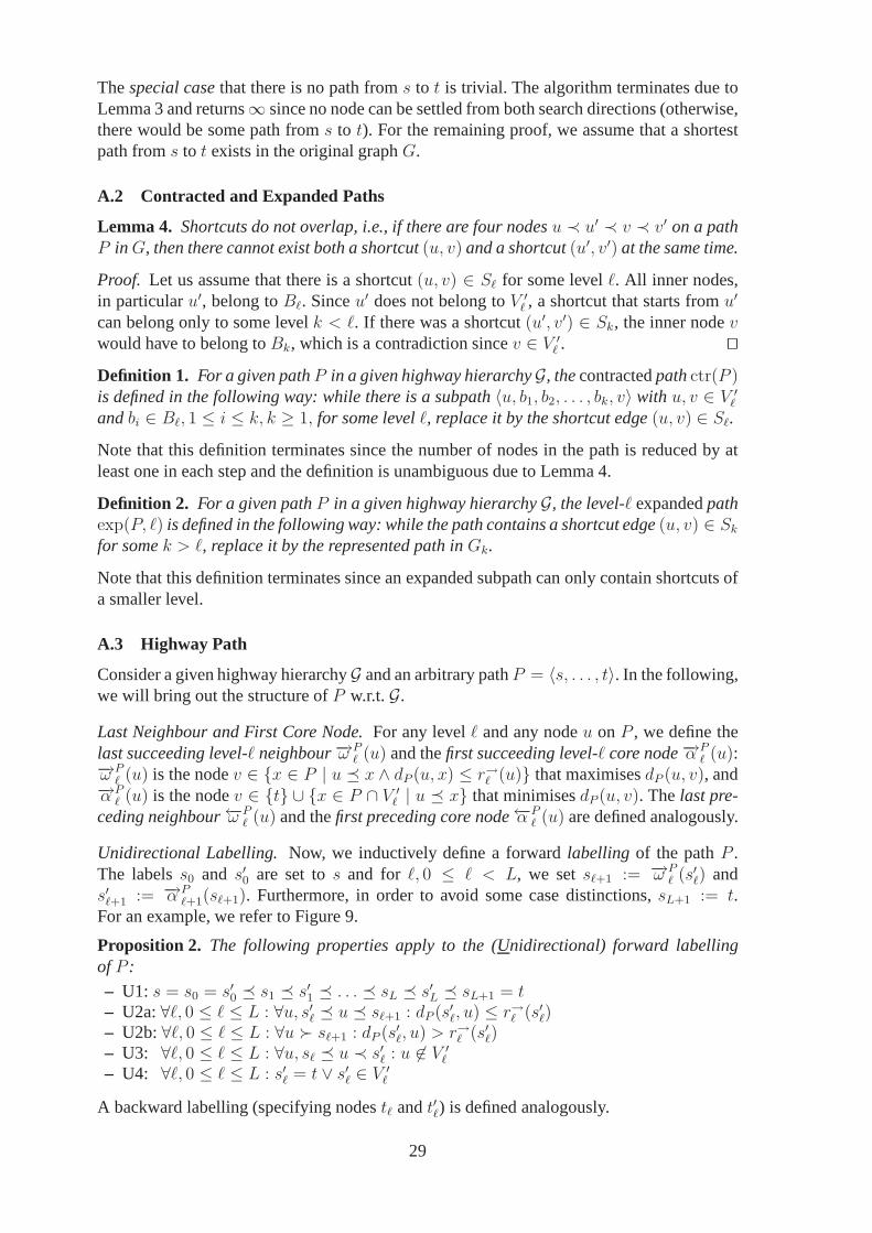
Thespecial casethat there is no path froms to t is trivial. The algorithm terminates due toLemma 3 and returns∞ since no node can be settled from both search directions (otherwise,there would be some path froms to t). For the remaining proof, we assume that a shortestpath froms to t exists in the original graphG.

A.2 Contracted and Expanded Paths

Lemma 4. Shortcuts do not overlap, i.e., if there are four nodesu ≺ u′ ≺ v ≺ v′ on a pathP in G, then there cannot exist both a shortcut(u, v) and a shortcut(u′, v′) at the same time.

Proof. Let us assume that there is a shortcut(u, v) ∈ Sℓ for some levelℓ. All inner nodes,in particularu′, belong toBℓ. Sinceu′ does not belong toV ′ℓ , a shortcut that starts fromu′

can belong only to some levelk < ℓ. If there was a shortcut(u′, v′) ∈ Sk, the inner nodevwould have to belong toBk, which is a contradiction sincev ∈ V ′ℓ . ⊓⊔Definition 1. For a given pathP in a given highway hierarchyG, thecontractedpathctr(P )is defined in the following way: while there is a subpath〈u, b1, b2, . . . , bk, v〉 with u, v ∈ V ′ℓandbi ∈ Bℓ, 1 ≤ i ≤ k, k ≥ 1, for some levelℓ, replace it by the shortcut edge(u, v) ∈ Sℓ.

Note that this definition terminates since the number of nodes in the path is reduced by atleast one in each step and the definition is unambiguous due toLemma 4.

Definition 2. For a given pathP in a given highway hierarchyG, the level-ℓ expandedpathexp(P, ℓ) is defined in the following way: while the path contains a shortcut edge(u, v) ∈ Sk

for somek > ℓ, replace it by the represented path inGk.

Note that this definition terminates since an expanded subpath can only contain shortcuts ofa smaller level.

A.3 Highway Path

Consider a given highway hierarchyG and an arbitrary pathP = 〈s, . . . , t〉. In the following,we will bring out the structure ofP w.r.t.G.

Last Neighbour and First Core Node.For any levelℓ and any nodeu on P , we define thelast succeeding level-ℓ neighbour−→ω P

ℓ (u) and thefirst succeeding level-ℓ core node−→α Pℓ (u):

−→ω Pℓ (u) is the nodev ∈ {x ∈ P | u � x ∧ dP (u, x) ≤ r→ℓ (u)} that maximisesdP (u, v), and−→α P

ℓ (u) is the nodev ∈ {t} ∪ {x ∈ P ∩ V ′ℓ | u � x} that minimisesdP (u, v). Thelast pre-ceding neighbour←−ω P

ℓ (u) and thefirst preceding core node←−α Pℓ (u) are defined analogously.

Unidirectional Labelling. Now, we inductively define a forwardlabelling of the pathP .The labelss0 and s′0 are set tos and for ℓ, 0 ≤ ℓ < L, we setsℓ+1 := −→ω P

ℓ (s′ℓ) ands′ℓ+1 := −→α P

ℓ+1(sℓ+1). Furthermore, in order to avoid some case distinctions,sL+1 := t.For an example, we refer to Figure 9.

Proposition 2. The following properties apply to the (Unidirectional) forward labellingof P :

– U1: s = s0 = s′0 � s1 � s′1 � . . . � sL � s′L � sL+1 = t– U2a:∀ℓ, 0 ≤ ℓ ≤ L : ∀u, s′ℓ � u � sℓ+1 : dP (s′ℓ, u) ≤ r→ℓ (s′ℓ)– U2b:∀ℓ, 0 ≤ ℓ ≤ L : ∀u ≻ sℓ+1 : dP (s′ℓ, u) > r→ℓ (s′ℓ)– U3: ∀ℓ, 0 ≤ ℓ ≤ L : ∀u, sℓ � u ≺ s′ℓ : u 6∈ V ′ℓ– U4: ∀ℓ, 0 ≤ ℓ ≤ L : s′ℓ = t ∨ s′ℓ ∈ V ′ℓ

A backward labelling (specifying nodestℓ andt′ℓ) is defined analogously.

29

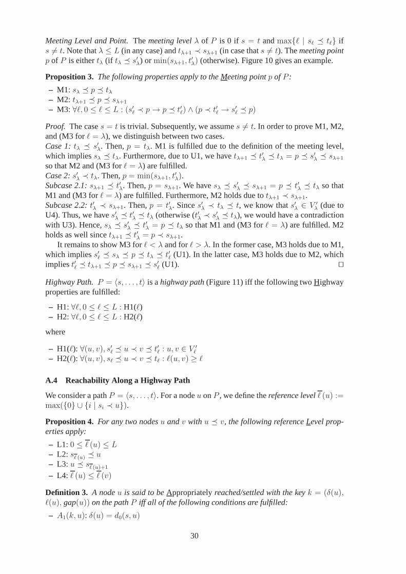
Meeting Level and Point.Themeeting levelλ of P is 0 if s = t andmax{ℓ | sℓ � tℓ} ifs 6= t. Note thatλ ≤ L (in any case) andtλ+1 ≺ sλ+1 (in case thats 6= t). Themeeting pointp of P is eithertλ (if tλ � s′λ) or min(sλ+1, t

′λ) (otherwise). Figure 10 gives an example.

Proposition 3. The following properties apply to the Meeting pointp of P :

– M1: sλ � p � tλ– M2: tλ+1 � p � sλ+1

– M3: ∀ℓ, 0 ≤ ℓ ≤ L : (s′ℓ ≺ p→ p � t′ℓ) ∧ (p ≺ t′ℓ → s′ℓ � p)

Proof. The cases = t is trivial. Subsequently, we assumes 6= t. In order to prove M1, M2,and (M3 forℓ = λ), we distinguish between two cases.Case 1:tλ � s′λ. Then,p = tλ. M1 is fulfilled due to the definition of the meeting level,which impliessλ � tλ. Furthermore, due to U1, we havetλ+1 � t′λ � tλ = p � s′λ � sλ+1

so that M2 and (M3 forℓ = λ) are fulfilled.Case 2:s′λ ≺ tλ. Then,p = min(sλ+1, t

′λ).

Subcase 2.1:sλ+1 � t′λ. Then,p = sλ+1. We havesλ � s′λ � sλ+1 = p � t′λ � tλ so thatM1 and (M3 forℓ = λ) are fulfilled. Furthermore, M2 holds due totλ+1 ≺ sλ+1.Subcase 2.2:t′λ ≺ sλ+1. Then,p = t′λ. Sinces′λ ≺ tλ � t, we know thats′λ ∈ V ′λ (due toU4). Thus, we haves′λ � t′λ � tλ (otherwise (t′λ ≺ s′λ � tλ), we would have a contradictionwith U3). Hence,sλ � s′λ � t′λ = p � tλ so that M1 and (M3 forℓ = λ) are fulfilled. M2holds as well sincetλ+1 � t′λ = p ≺ sλ+1.

It remains to show M3 forℓ < λ and forℓ > λ. In the former case, M3 holds due to M1,which impliess′ℓ � sλ � p � tλ � t′ℓ (U1). In the latter case, M3 holds due to M2, whichimpliest′ℓ � tλ+1 � p � sλ+1 � s′ℓ (U1). ⊓⊔

Highway Path.P = 〈s, . . . , t〉 is ahighway path(Figure 11) iff the following two Highwayproperties are fulfilled:

– H1: ∀ℓ, 0 ≤ ℓ ≤ L : H1(ℓ)– H2: ∀ℓ, 0 ≤ ℓ ≤ L : H2(ℓ)

where

– H1(ℓ): ∀(u, v), s′ℓ � u ≺ v � t′ℓ : u, v ∈ V ′ℓ– H2(ℓ): ∀(u, v), sℓ � u ≺ v � tℓ : ℓ(u, v) ≥ ℓ

A.4 Reachability Along a Highway Path

We consider a pathP = 〈s, . . . , t〉. For a nodeu onP , we define thereference levelℓ (u) :=max({0} ∪ {i | si ≺ u}).

Proposition 4. For any two nodesu andv with u � v, the following reference Level prop-erties apply:

– L1: 0 ≤ ℓ (u) ≤ L– L2: sℓ (u) � u– L3: u � sℓ (u)+1

– L4: ℓ (u) ≤ ℓ (v)

Definition 3. A nodeu is said to beAppropriatelyreached/settled with the keyk = (δ(u),ℓ(u), gap(u)) on the pathP iff all of the following conditions are fulfilled:

– A1(k, u): δ(u) = d0(s, u)

30

– A2(k, u): ℓ(u) = ℓ (u)

– A3(k, u): gap(u) =

{∞ if u � s′ℓ(u)

r→ℓ(u)(s′

ℓ(u))− dP (s′ℓ(u), u) otherwise– A4(u): ∀i : t 6= s′i � u→ u ∈ V ′i

The following (somewhat technical) lemma will be used to prove Lemmas 6 and 7. Basi-cally, it states that in the highway query algorithm the search level and the gap to the nextapplicable neighbourhood border are set correctly.

Lemma 5. Consider a pathP = 〈s, . . . , t〉 and an edge(u, v) onP . Assume thatu is settledby the highway query algorithm appropriately with some keyk. We consider the attempt torelax the edge(u, v). After Line 9 has been executed, the following Invariants apply w.r.t.the variablesℓ and gap:

– I1: (a) sℓ � u ∧ (b) v � sℓ+1

– I2: ℓ = ℓ (v)

– I3: gap=

{∞ if v � s′ℓ,r→ℓ (s′ℓ)− dP (s′ℓ, u) otherwise.

Proof. We distinguish between two cases in order to prove I1 and I3.Case 1:zero iterations of the for-loop in Line 9 take place (ℓ = ℓ(u)).In this case, we haveℓ = ℓ(u) andw(u, v) ≤ gap′. Hence,sℓ � u due toA2(k, u) and L2(⇒ I1a). In order to show I1b and I3, we distinguish between three subcases:

– Subcase 1.1:u ≺ s′ℓ⇒ v � s′ℓ � sℓ+1 (U1) (⇒ I1b). Furthermore, because of gap(u) =∞ (A3(u, k)), we have gap= gap′ = r→ℓ(u)(u) = ∞ due to U3 and R1 (⇒ I3 sincev � s′ℓ).

– Subcase 1.2:u = s′ℓ ⇒ gap(u) = ∞ (A3(u, k))⇒ w(u, v) ≤ gap′ = r→ℓ (u) (Line 7)⇒ dP (s′ℓ, v) ≤ r→ℓ (s′ℓ) (sinceu = s′ℓ)⇒ v � sℓ+1 (U2b) (⇒ I1b). Furthermore, gap=gap′ = r→ℓ (u) = r→ℓ (s′ℓ)− dP (s′ℓ, u) (sinceu = s′ℓ) implies I3 sinces′ℓ ≺ v.

– Subcase 1.3:u ≻ s′ℓ ⇒ gap(u) = r→ℓ (s′ℓ) − dP (s′ℓ, u) (A3(u, k)). By Lemma 2,ℓ ≤ Land (ℓ = L → gap = ∞). If ℓ = L, we havev � t = sL+1 = sℓ+1 (⇒ I1b) andgap= ∞ = r→ℓ (s′ℓ) − dP (s′ℓ, u) (R2) (⇒ I3 sinces′ℓ ≺ v). Subsequently, we deal withthe remaining caseℓ < L. The facts thatu � t ands′ℓ ≺ u imply s′ℓ 6= t, which yieldss′ℓ ∈ V ′ℓ due to U4. Hence, due to R3, gap(u) 6=∞⇒ w(u, v) ≤ gap′ = gap(u) (Line 7)⇒ dP (u, v) ≤ r→ℓ (s′ℓ) − dP (s′ℓ, u)⇒ dP (s′ℓ, v) ≤ r→ℓ (s′ℓ)⇒ v � sℓ+1 (U2b) (⇒ I1b).Furthermore, gap= gap′ = gap(u) = r→ℓ (s′ℓ)− dP (s′ℓ, u) implies I3 sinces′ℓ ≺ v.

Case 2:at least one iteration of the for-loop takes place (ℓ > ℓ(u)).We claim that after any iteration of the for-loop, we haveu = sℓ. Proof by induction:Base Case:We consider the first iteration of the for-loop. Line 9 and thefact that an iterationtakes place implyw(u, v) > gap′, which means that gap′ 6=∞. We distinguish between twosubcases to show thatdP (s′ℓ(u), v) > r→ℓ(u)(s

′

ℓ(u)).

– Subcase 2.1:u � s′ℓ(u)⇒ gap(u) =∞ (A3(u, k))⇒ w(u, v) > gap′ = r→ℓ(u)(u) (Line 7)⇒ r→ℓ(u)(u) 6= ∞. We havesℓ(u) � u � s′ℓ(u) due to L2,A2(u, k), and the assumption ofSubcase 2.1. However, we can exclude thatsℓ(u) � u ≺ s′ℓ(u): this would implyu 6∈ V ′ℓ(u)

(U3) and, thus,r→ℓ(u)(u) =∞ (R1). Therefore,u = s′ℓ(u)⇒ dP (s′ℓ(u), v) > r→ℓ(u)(s′

ℓ(u))

– Subcase 2.2:u ≻ s′ℓ(u) ⇒ s′ℓ(u) 6= t ⇒ s′ℓ(u) ∈ V ′ℓ(u) (U4). Furthermore, gap(u) =

r→ℓ(u)(s′

ℓ(u))−dP (s′ℓ(u), u) (A3(u, k))⇒ gap(u) 6=∞ (due to R3 sinceℓ(u) < L (Lemma 2)ands′ℓ(u) ∈ V ′ℓ(u))⇒ dP (u, v) = w(u, v) > gap′ = gap(u) = r→ℓ(u)(s

′

ℓ(u)) − dP (s′ℓ(u), u)

(Line 7)⇒ dP (s′ℓ(u), v) > r→ℓ(u)(s′

ℓ(u))

31

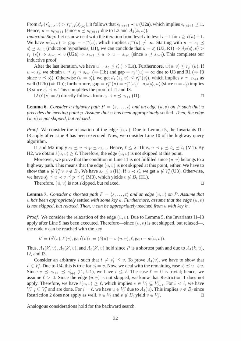
FromdP (s′ℓ(u), v) > r→ℓ(u)(s′

ℓ(u)), it follows thatsℓ(u)+1 ≺ v (U2a), which impliessℓ(u)+1 � u.Hence,u = sℓ(u)+1 (sinceu � sℓ(u)+1 due to L3 andA2(k, u)).Induction Step:Let us now deal with the iteration from leveli to leveli+1 for i ≥ ℓ(u)+1.We havew(u, v) > gap = r→i (u), which impliesr→i (u) 6= ∞. Starting withu = si �s′i � si+1 (induction hypothesis, U1), we can conclude thatu = s′i (U3, R1)⇒ dP (s′i, v) >r→i (s′i)⇒ si+1 ≺ v (U2a)⇒ si+1 � u⇒ u = si+1 (sinceu � si+1). This completes ourinductive proof.

After the last iteration, we haveu = sℓ � s′ℓ (⇒ I1a). Furthermore,w(u, v) ≤ r→ℓ (u). Ifu ≺ s′ℓ, we obtainv � s′ℓ � sℓ+1 (⇒ I1b) and gap= r→ℓ (u) = ∞ due to U3 and R1 (⇒ I3sincev � s′ℓ). Otherwise (u = s′ℓ), we getdP (s′ℓ, v) ≤ r→ℓ (s′ℓ), which impliesv � sℓ+1 aswell (U2b) (⇒ I1b); furthermore, gap= r→ℓ (u) = r→ℓ (s′ℓ)−dP (s′ℓ, u) (sinceu = s′ℓ) impliesI3 sinces′ℓ ≺ v. This completes the proof of I1 and I3.

I2 (ℓ (v) = ℓ) directly follows fromsℓ ≺ v � sℓ+1 (I1). ⊓⊔

Lemma 6. Consider a highway pathP = 〈s, . . . , t〉 and an edge(u, v) on P such thatuprecedes the meeting pointp. Assume thatu has been appropriatelysettled. Then, the edge(u, v) is not skipped, but relaxed.

Proof. We consider the relaxation of the edge(u, v). Due to Lemma 5, the Invariants I1–I3 apply after Line 9 has been executed. Now, we consider Line10 of the highway queryalgorithm.

I1 and M2 implysℓ � u ≺ p � sλ+1. Hence,ℓ ≤ λ. Thus,u ≺ p � tλ � tℓ (M1). ByH2, we obtainℓ(u, v) ≥ ℓ. Therefore, the edge(u, v) is not skipped at this point.

Moreover, we prove that the condition in Line 11 is not fulfilled since(u, v) belongs to ahighway path. This means that the edge(u, v) is not skipped at this point, either. We have toshow thatu 6∈ V ′ℓ ∨ v 6∈ Bℓ. We havesℓ � u (I1). If u ≺ s′ℓ, we getu 6∈ V ′ℓ (U3). Otherwise,we haves′ℓ � u ≺ v � p � t′ℓ (M3), which yieldsv 6∈ Bℓ (H1).

Therefore,(u, v) is not skipped, but relaxed. ⊓⊔

Lemma 7. Consider a shortest pathP = 〈s, . . . , t〉 and an edge(u, v) on P . Assume thatu has been appropriatelysettledwith some keyk. Furthermore, assume that the edge(u, v)is not skipped, but relaxed. Then,v can be appropriatelyreachedfromu with keyk′.

Proof. We consider the relaxation of the edge(u, v). Due to Lemma 5, the Invariants I1–I3apply after Line 9 has been executed. Therefore—since(u, v) is not skipped, but relaxed—,the nodev can be reached with the key

k′ = (δ′(v), ℓ′(v), gap′(v)) := (δ(u) + w(u, v), ℓ, gap− w(u, v)).

Thus,A1(k′, v), A2(k

′, v), andA3(k′, v) hold sinceP is a shortest path and due toA1(k, u),

I2, and I3.Consider an arbitraryi such thatt 6= s′i � v. To proveA4(v), we have to show that

v ∈ V ′i . Due to U4, this is true fors′i = v. Now, we deal with the remaining cases′i � u ≺ v.Sincev � sℓ+1 � s′ℓ+1 (I1, U1), we havei ≤ ℓ. The caseℓ = 0 is trivial; hence, weassumeℓ > 0. Since the edge(u, v) is not skipped, we know that Restriction 1 does notapply. Therefore, we haveℓ(u, v) ≥ ℓ, which impliesv ∈ Vℓ ⊆ V ′ℓ−1. For i < ℓ, we haveV ′ℓ−1 ⊆ V ′i and are done. Fori = ℓ, we haveu ∈ V ′ℓ due toA4(u). This impliesv 6∈ Bℓ sinceRestriction 2 does not apply as well.v ∈ Vℓ andv 6∈ Bℓ yield v ∈ V ′ℓ . ⊓⊔

Analogous considerations hold for the backward search.

32

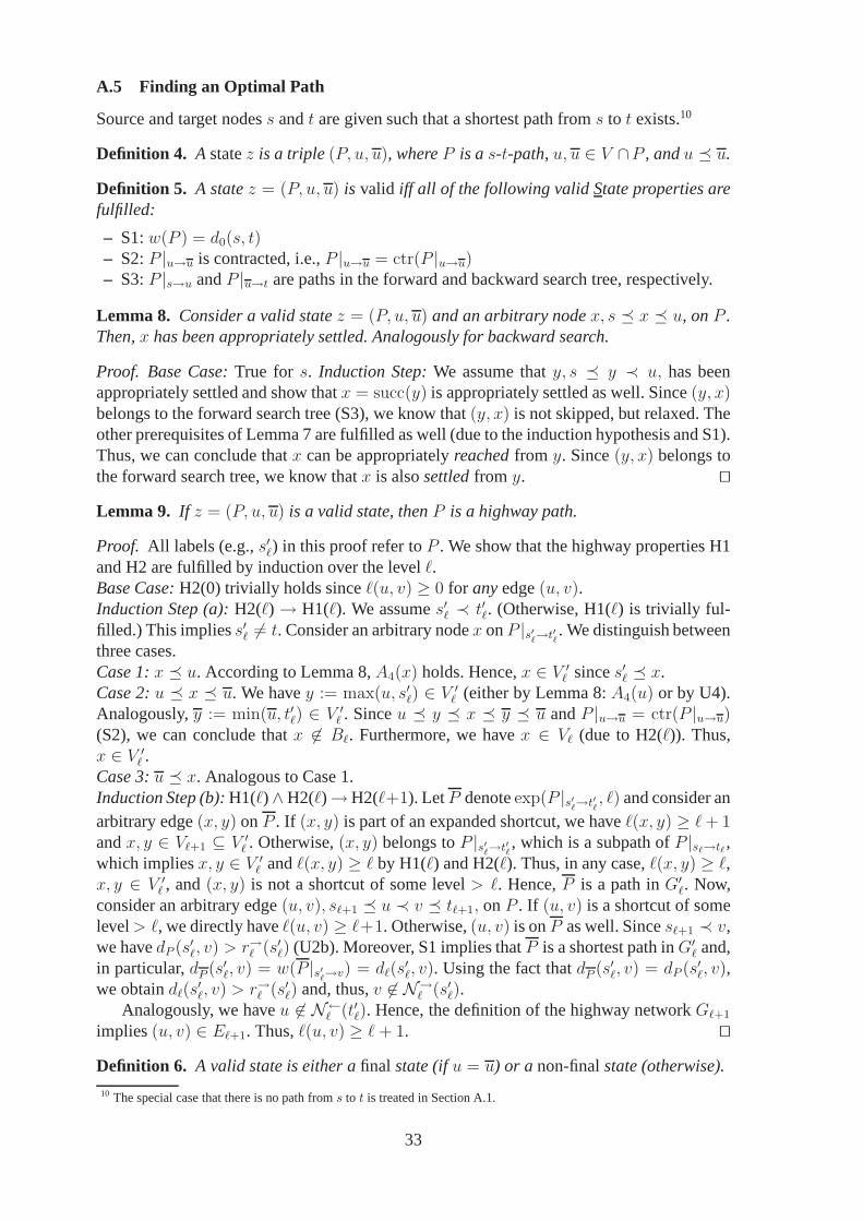
A.5 Finding an Optimal Path

Source and target nodess andt are given such that a shortest path froms to t exists.10

Definition 4. A statez is a triple(P, u, u), whereP is as-t-path,u, u ∈ V ∩P , andu � u.

Definition 5. A statez = (P, u, u) is valid iff all of the following valid State properties arefulfilled:

– S1:w(P ) = d0(s, t)– S2:P |u→u is contracted, i.e.,P |u→u = ctr(P |u→u)– S3:P |s→u andP |u→t are paths in the forward and backward search tree, respectively.

Lemma 8. Consider a valid statez = (P, u, u) and an arbitrary nodex, s � x � u, onP .Then,x has been appropriately settled. Analogously for backward search.

Proof. Base Case:True for s. Induction Step:We assume thaty, s � y ≺ u, has beenappropriately settled and show thatx = succ(y) is appropriately settled as well. Since(y, x)belongs to the forward search tree (S3), we know that(y, x) is not skipped, but relaxed. Theother prerequisites of Lemma 7 are fulfilled as well (due to the induction hypothesis and S1).Thus, we can conclude thatx can be appropriatelyreachedfrom y. Since(y, x) belongs tothe forward search tree, we know thatx is alsosettledfrom y. ⊓⊔

Lemma 9. If z = (P, u, u) is a valid state, thenP is a highway path.

Proof. All labels (e.g.,s′ℓ) in this proof refer toP . We show that the highway properties H1and H2 are fulfilled by induction over the levelℓ.Base Case:H2(0) trivially holds sinceℓ(u, v) ≥ 0 for anyedge(u, v).Induction Step (a):H2(ℓ)→ H1(ℓ). We assumes′ℓ ≺ t′ℓ. (Otherwise, H1(ℓ) is trivially ful-filled.) This impliess′ℓ 6= t. Consider an arbitrary nodex onP |s′

ℓ→t′

ℓ. We distinguish between

three cases.Case 1:x � u. According to Lemma 8,A4(x) holds. Hence,x ∈ V ′ℓ sinces′ℓ � x.Case 2:u � x � u. We havey := max(u, s′ℓ) ∈ V ′ℓ (either by Lemma 8:A4(u) or by U4).Analogously,y := min(u, t′ℓ) ∈ V ′ℓ . Sinceu � y � x � y � u andP |u→u = ctr(P |u→u)(S2), we can conclude thatx 6∈ Bℓ. Furthermore, we havex ∈ Vℓ (due to H2(ℓ)). Thus,x ∈ V ′ℓ .Case 3:u � x. Analogous to Case 1.Induction Step (b):H1(ℓ)∧H2(ℓ)→H2(ℓ+1). LetP denoteexp(P |s′

ℓ→t′

ℓ, ℓ) and consider an

arbitrary edge(x, y) onP . If (x, y) is part of an expanded shortcut, we haveℓ(x, y) ≥ ℓ + 1andx, y ∈ Vℓ+1 ⊆ V ′ℓ . Otherwise,(x, y) belongs toP |s′

ℓ→t′

ℓ, which is a subpath ofP |sℓ→tℓ,

which impliesx, y ∈ V ′ℓ andℓ(x, y) ≥ ℓ by H1(ℓ) and H2(ℓ). Thus, in any case,ℓ(x, y) ≥ ℓ,x, y ∈ V ′ℓ , and(x, y) is not a shortcut of some level> ℓ. Hence,P is a path inG′ℓ. Now,consider an arbitrary edge(u, v), sℓ+1 � u ≺ v � tℓ+1, onP . If (u, v) is a shortcut of somelevel> ℓ, we directly haveℓ(u, v) ≥ ℓ+1. Otherwise,(u, v) is onP as well. Sincesℓ+1 ≺ v,we havedP (s′ℓ, v) > r→ℓ (s′ℓ) (U2b). Moreover, S1 implies thatP is a shortest path inG′ℓ and,in particular,dP (s′ℓ, v) = w(P |s′

ℓ→v) = dℓ(s

′ℓ, v). Using the fact thatdP (s′ℓ, v) = dP (s′ℓ, v),

we obtaindℓ(s′ℓ, v) > r→ℓ (s′ℓ) and, thus,v 6∈ N→ℓ (s′ℓ).

Analogously, we haveu 6∈ N←ℓ (t′ℓ). Hence, the definition of the highway networkGℓ+1

implies(u, v) ∈ Eℓ+1. Thus,ℓ(u, v) ≥ ℓ + 1. ⊓⊔

Definition 6. A valid state is either afinal state (ifu = u) or a non-finalstate (otherwise).

10 The special case that there is no path froms to t is treated in Section A.1.

33

We pick any shortests-t-pathP . The state(ctr(P ), s, t) is the initial state. Since forwardand backward search run completely independently of each other, any serialisation of bothsearch processes will yield exactly the same result. Therefore, in our proof, we are freeto pick—w.l.o.g.—any order of forward and backward steps. We assume that at first oneforward and one backward iteration is performed, which implies thats andt are settled. Atthis point, the highway query algorithm is in the initial state. It is easy to see that the initialstate is a valid state. Due to the following lemma, it is sufficient to prove that a final state iseventually reached.

Lemma 10. Getting to a final state is equivalent to finding a shortests-t-path.

Proof. u = u means that forward and backward search meet. Due to Lemma 8, we canconclude that bothu andu are settled with the optimal distance (A1), i.e.,

−→δ (u) = d0(s, u)

and←−δ (u) = d0(u, t). Sinceu = u lies on a shortest path (due to S1), we haved(s, t) =

d0(s, u) + d0(u, t). Line 6 impliesd′ ≤ −→δ (u) +←−δ (u) = d(s, t). In fact, this means that the

algorithm returnsd′ = d(s, t) since this is already optimal. ⊓⊔

Definition 7. For a valid statez = (P, u, u), the forward direction is said to beblockedifp � u. Analogously, the backward direction is blocked ifu � p.

Lemma 11. For a non-final statez = (P, u, u), at most one direction is blocked.

Proof. Sincez is a non-final state, we haveu ≺ u, which impliesu ≺ p or p ≺ u. ⊓⊔

Definition 8. Therankρ(z) of a statez = (P, u, u) is |{x ∈ P | u � x � u}|.

Lemma 12. From any non-final statez = (P, u, u), another valid statez+ is reached atsome point such thatρ(z+) < ρ(z).

Proof. We pick any non-blocked direction—due to Lemma 11, we know that there is atleast one such direction. Subsequently, we assume that the forward direction was picked;the backward direction can be dealt with analogously.

We haveu ≺ p and observe that all prerequisites of Lemma 6 are fulfilled due to Lem-mas 9 and 8. Hence, we can conclude that the edge(u, v := succ(u)) is not skipped, butrelaxed. Thus, sinceP is a shortest path (S1),v can be reached with the optimal distance dueto Lemma 7 (A1). The fact that the algorithm terminates (Lemma 3) implies that the queue

−→Q

gets empty at some point, i.e., every element has been deleted from−→Q . In particular, we can

conclude thatv is deleted at some point. Sincev has been reached with the optimal distance,it will also be settled with the optimal distance (due to the specification of the decreaseKeyoperation, which guarantees that tentative distances are never increased). LetP ′ denote thepath froms to v in the forward search tree. We setz+ := (P+ := P ′ ◦P |v→t, v, u). We havew(P+) = w(P ′) + w(P |v→t) = d0(s, v) + d0(v, t) = d0(s, t) (⇒ S1). S2 is fulfilled sinceP+|v→u is a subpath ofP |u→u. S3 holds due to the construction ofP+. Hence,z+ is valid.Furthermore,ρ(z+) = ρ(z)− 1. ⊓⊔

Theorem 5. The highway query algorithm finds a shortests-t-path.

Proof. From Lemma 12 and the fact that the codomain of the rank function is finite, itfollows that eventually a final state is reached, which is equivalent to finding a shortests-t-path due to Lemma 10. ⊓⊔

34

A.6 Distance Table Optimisation

To prove the correctness of the distance table optimisation, we introduce the following newlemma and adapt a few definitions and proofs from Section A.5 to the new situation.

Lemma 13. Consider a valid statez = (P, u, u) with u ≺ s′L. Whenu’s edges are relaxed,neither the condition in Line 7a nor the condition in Line 11ais fulfilled.

Proof. Due to Lemma 8,u has been appropriately settled with some keyk. We distinguishbetween two cases.Case 1:u ≺ sL. Fromsℓ(u) = sℓ (u) � u ≺ sL (A2(k, u), L2), it follows thatℓ(u) < L (U1).Hence, the condition in Line 7a is not fulfilled. Furthermore, we havesℓ � u ≺ sL afterLine 9 has been executed (Lemma 5: I1). Thus,ℓ < L, which implies that the condition inLine 11a is not fulfilled as well.Case 2:sL � u ≺ s′L. First, we show that the condition in Line 7a is not fulfilled.Weassumeℓ(u) = L. (Otherwise, the condition cannot be fulfilled.) Due toA3(k, u), we havegap(u) = ∞. Hence, gap′ = r→ℓ(u)(u) = r→L (u) = ∞1 by R1 sinceu 6∈ V ′L (U3). Now, weprove that the condition in Line 11a is not fulfilled. We assumeℓ = L∧ℓ > ℓ(u). (Otherwise,the condition cannot be fulfilled.) Due to Line 9, we get gap= r→ℓ (u) = r→L (u) = ∞1 (asabove). ⊓⊔Definition 6’. A valid state is either afinal state (ifu = u or s′L � u∧u � t′L) or a non-finalstate (otherwise).

Lemma 10.Getting to a final state is equivalent to finding a shortests-t-path.

Proof. In the proof of this lemma in Section A.5, we have already dealt with the caseu = u.Now, consider the new caseu ≺ u ∧ s′L � u ∧ u � t′L. We show thats′L is added to theset−→I . Sinces′L � u, s′L has been appropriately settled with some keyk (due to Lemma 8).

We consider the attempt to relax the edge(s′L, v := succ(s′L)) and distinguish between twocases.Case 1:sL = s′L. ℓ = ℓ (v) (I2), sL = s′L ≺ v, andℓ (v) ≤ L (L1) imply ℓ = ℓ (v) = L.Furthermore,A2(k, s′L) and the assumption of Case 1 yieldℓ(s′L) = ℓ (s′L) < L = ℓ. Inaddition, gap=∞2 6=∞1 by I3 (sinces′ℓ ≺ v), the fact thats′L ∈ V ′L (U4), and R2. Hence,the condition in Line 11a is fulfilled so thats′L is added to

−→I .

Case 2:sL ≺ s′L. By A2(k, s′L), A3(k, s′L), the assumption of Case 2, andℓ (s′L) ≤ L (L1),we getℓ(s′L) = ℓ (s′L) = L and gap(s′L) = ∞. Thus, gap′ = r→L (s′L) = ∞2 6= ∞1 (R2).Hence, the condition in Line 7a is fulfilled so thats′L is added to

−→I .

Analogously, we can prove thatt′L is added to the set←−I . SinceP is a highway path

(due to Lemma 9), the subpathP |s′L→t′

Lis a path inG′L and, thus,d0(s

′L, t′L) = dL(s′L, t′L).

Hence,w(P ) = d0(s, s′L) + dL(s′L, t′L) + d0(t

′L, t) is the length of a shortests-t-path and,

since the algorithm finds a path with a length≤ −→δ (s′L) + dL(s′L, t′L) +←−δ (t′L) and since−→

δ (s′L) = d0(s, s′L) and

←−δ (t′L) = d0(t

′L, t) (due to Lemma 8:A1), we can conclude that a

shortests-t-path is found. ⊓⊔Definition 7’. For a valid statez = (P, u, u), the forward direction is said to beblockedifp � u or s′L � u. Analogously, the backward direction is blocked ifu � p or u � t′L.

Lemma 11.For a non-final statez = (P, u, u), at most one direction is blocked.

Proof. Sincez is a non-final state, we haveu ≺ u and(u ≺ s′L ∨ t′L ≺ u). To obtain acontradiction, let us assume that both directions are blocked, i.e., (p � u or s′L � u) and

35

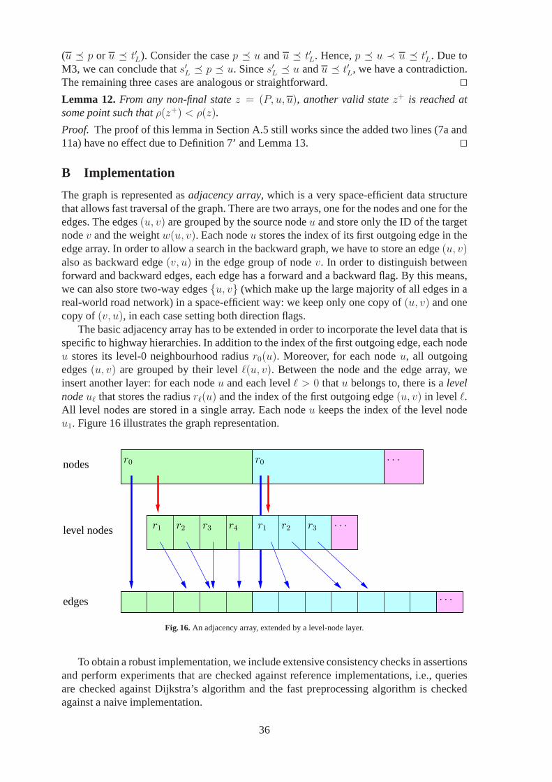
(u � p or u � t′L). Consider the casep � u andu � t′L. Hence,p � u ≺ u � t′L. Due toM3, we can conclude thats′L � p � u. Sinces′L � u andu � t′L, we have a contradiction.The remaining three cases are analogous or straightforward. ⊓⊔Lemma 12. From any non-final statez = (P, u, u), another valid statez+ is reached atsome point such thatρ(z+) < ρ(z).

Proof. The proof of this lemma in Section A.5 still works since the added two lines (7a and11a) have no effect due to Definition 7’ and Lemma 13. ⊓⊔

B Implementation

The graph is represented asadjacency array, which is a very space-efficient data structurethat allows fast traversal of the graph. There are two arrays, one for the nodes and one for theedges. The edges(u, v) are grouped by the source nodeu and store only the ID of the targetnodev and the weightw(u, v). Each nodeu stores the index of its first outgoing edge in theedge array. In order to allow a search in the backward graph, we have to store an edge(u, v)also as backward edge(v, u) in the edge group of nodev. In order to distinguish betweenforward and backward edges, each edge has a forward and a backward flag. By this means,we can also store two-way edges{u, v} (which make up the large majority of all edges in areal-world road network) in a space-efficient way: we keep only one copy of(u, v) and onecopy of(v, u), in each case setting both direction flags.

The basic adjacency array has to be extended in order to incorporate the level data that isspecific to highway hierarchies. In addition to the index of the first outgoing edge, each nodeu stores its level-0 neighbourhood radiusr0(u). Moreover, for each nodeu, all outgoingedges(u, v) are grouped by their levelℓ(u, v). Between the node and the edge array, weinsert another layer: for each nodeu and each levelℓ > 0 thatu belongs to, there is alevelnodeuℓ that stores the radiusrℓ(u) and the index of the first outgoing edge(u, v) in level ℓ.All level nodes are stored in a single array. Each nodeu keeps the index of the level nodeu1. Figure 16 illustrates the graph representation.

r0nodes

level nodes

edges

· · ·

· · ·

r0

r1 r2 r3 r4 r3r2r1 · · ·

Fig. 16.An adjacency array, extended by a level-node layer.

To obtain a robust implementation, we include extensive consistency checks in assertionsand perform experiments that are checked against referenceimplementations, i.e., queriesare checked against Dijkstra’s algorithm and the fast preprocessing algorithm is checkedagainst a naive implementation.

36

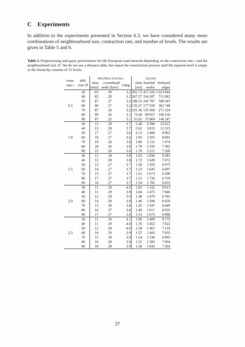
C Experiments

In addition to the experiments presented in Section 6.3, we have considered many morecombinations of neighbourhood size, contraction rate, andnumber of levels. The results aregiven in Table 5 and 6.

Table 5.Preprocessing and query performance for the European road network depending on the contraction ratec and theneighbourhood sizeH . We do not use a distance table, but repeat the construction process until the topmost level is emptyor the hierarchy consists of 15 levels.

contr. nbh.PREPROCESSING QUERY

ratec sizeHtime ∅overhead/

∅deg.time #settled #relaxed

[min] node [byte] [ms] nodes edges

0.5

30 83 30 3.2391.73 472 326 1 023 94440 83 28 3.2267.57 334 287 711 08250 87 27 3.2188.55 242 787 506 54360 86 27 3.2135.27 177 558 362 74870 87 26 3.2101.36 135 560 271 32480 89 26 3.1 73.40 99 857 196 15090 87 25 3.1 55.02 75 969 146 247

1.0

30 15 28 3.7 5.48 6 396 23 61240 15 28 3.7 2.62 3 033 11 31550 17 27 3.6 2.13 2 406 8 90260 18 27 3.6 1.93 2 201 8 00170 19 26 3.6 1.80 2 151 7 47480 20 26 3.6 1.79 2 193 7 39290 22 26 3.6 1.78 2 221 7 268

1.5

30 11 28 3.8 1.93 1 830 9 28140 12 28 3.8 1.72 1 628 7 67250 13 27 3.7 1.56 1 593 6 97560 14 27 3.7 1.53 1 645 6 69770 15 27 3.7 1.51 1 673 6 59080 17 27 3.7 1.51 1 726 6 71990 18 27 3.7 1.54 1 782 6 655

2.0

30 11 29 4.0 1.85 1 542 8 91340 11 29 3.9 1.64 1 475 7 64650 12 28 3.9 1.48 1 470 6 78560 14 28 3.8 1.46 1 506 6 65070 15 28 3.8 1.45 1 547 6 64980 16 27 3.8 1.49 1 611 6 93590 17 27 3.8 1.53 1 675 6 988

2.5

30 11 30 4.1 1.96 1 489 9 17540 11 29 4.0 1.70 1 453 7 82250 12 29 4.0 1.58 1 467 7 11960 14 29 3.9 1.57 1 493 7 03570 15 28 3.9 1.54 1 536 6 90580 16 28 3.9 1.55 1 583 7 09490 18 28 3.9 1.58 1 645 7 204

37

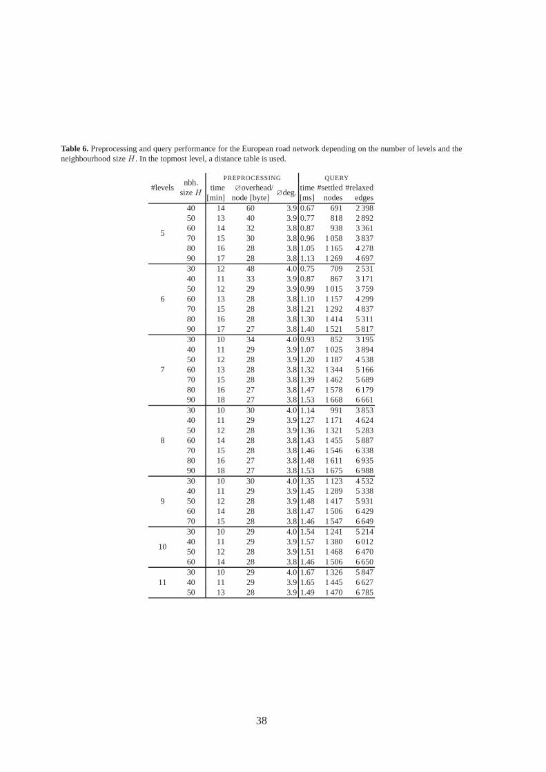
Table 6.Preprocessing and query performance for the European road network depending on the number of levels and theneighbourhood sizeH . In the topmost level, a distance table is used.

#levelsnbh.

PREPROCESSING QUERY

sizeHtime ∅overhead/

∅deg.time #settled #relaxed

[min] node [byte] [ms] nodes edges

5

40 14 60 3.90.67 691 2 39850 13 40 3.90.77 818 2 89260 14 32 3.80.87 938 3 36170 15 30 3.80.96 1 058 3 83780 16 28 3.81.05 1 165 4 27890 17 28 3.81.13 1 269 4 697

6

30 12 48 4.00.75 709 2 53140 11 33 3.90.87 867 3 17150 12 29 3.90.99 1 015 3 75960 13 28 3.81.10 1 157 4 29970 15 28 3.81.21 1 292 4 83780 16 28 3.81.30 1 414 5 31190 17 27 3.81.40 1 521 5 817

7

30 10 34 4.00.93 852 3 19540 11 29 3.91.07 1 025 3 89450 12 28 3.91.20 1 187 4 53860 13 28 3.81.32 1 344 5 16670 15 28 3.81.39 1 462 5 68980 16 27 3.81.47 1 578 6 17990 18 27 3.81.53 1 668 6 661

8

30 10 30 4.01.14 991 3 85340 11 29 3.91.27 1 171 4 62450 12 28 3.91.36 1 321 5 28360 14 28 3.81.43 1 455 5 88770 15 28 3.81.46 1 546 6 33880 16 27 3.81.48 1 611 6 93590 18 27 3.81.53 1 675 6 988

9

30 10 30 4.01.35 1 123 4 53240 11 29 3.91.45 1 289 5 33850 12 28 3.91.48 1 417 5 93160 14 28 3.81.47 1 506 6 42970 15 28 3.81.46 1 547 6 649

10

30 10 29 4.01.54 1 241 5 21440 11 29 3.91.57 1 380 6 01250 12 28 3.91.51 1 468 6 47060 14 28 3.81.46 1 506 6 650

1130 10 29 4.01.67 1 326 5 84740 11 29 3.91.65 1 445 6 62750 13 28 3.91.49 1 470 6 785

38