Engineering Fracture Mechanics - Yonsei...
24
Computational implementation of the PPR potential-based cohesive model in ABAQUS: Educational perspective Kyoungsoo Park a,⇑ , Glaucio H. Paulino b a School of Civil & Environmental Engineering, Yonsei University, 50 Yonsei-ro, Seodaemun-gu, Seoul, Republic of Korea b Department of Civil & Environmental Engineering, University of Illinois at Urbana–Champaign, 205 North Mathews Ave., Urbana, IL 61801, United States article info Article history: Received 2 August 2011 Received in revised form 9 February 2012 Accepted 9 February 2012 Keywords: Cohesive zone model PPR potential-based model Crack propagation Cohesive element abstract A potential-based cohesive zone model, so called the PPR model, is implemented in a com- mercial software, e.g. ABAQUS, as a user-defined element (UEL) subroutine. The intrinsic cohesive zone modeling approach is employed because it can be formulated within the standard finite element framework. The implementation procedure for a two-dimensional linear cohesive element and the algorithm for the PPR potential-based model are presented in-detail. The source code of the UEL subroutine is provided in Appendix for educational purposes. Three computational examples are investigated to verify the PPR model and its implementation. The computational results of the model agree well with the analytical solutions. Ó 2012 Elsevier Ltd. All rights reserved. 1. Introduction The cohesive zone model has been a powerful concept to approximate nonlinear fracture processes [1,2]. The concept of the cohesive zone model was presented by Barenblatt [3] and Dugdale [4]. Since then, the model has been utilized to inves- tigate a wide range of failure phenomena, which include, for example, fracture of quasi-brittle materials [5–8], bond-slip in reinforced concrete [9], delamination in adhesive bond joints [10,11], and matrix/particle debonding [12–14]. One of essential aspects in the cohesive zone model is the choice of a traction–separation relation. Because most traction– separation relationships display limitations, especially under mixed-mode conditions, the relationship should be selected with great caution [15]. Among various traction–separation relationships, the so-called PPR potential based model demon- strates the consistency of the constitutive relationship under mixed-mode conditions while considering different fracture energies with respect to fracture modes [15]. In order to benefit from the PPR potential-based model and capabilities of exist- ing commercial softwares for nonlinear fracture analysis, one could develop a user-defined element (UEL) subroutine for the PPR model in a commercial software such as ABAQUS [16]. Computational implementation of an existing algorithm (or model) may be a challenging task, especially for beginners in a new research area, because the detailed procedure or source codes are not generally provided in scientific journal papers. However, in order to facilitate research and to benefit from existing scientific contributions for researchers and engineers, there are several papers which address computational implementations. For instance, Sigmund [17] presented an implemen- tation of a topology optimization code for compliance minimization of statically loaded structures. Giner et al. [18] demon- strated an ABAQUS implementation of the extended finite element method as a UEL subroutine for linear elastic fracture analysis. 0013-7944/$ - see front matter Ó 2012 Elsevier Ltd. All rights reserved. http://dx.doi.org/10.1016/j.engfracmech.2012.02.007 ⇑ Corresponding author. Tel.: +82 2 2123 5806; fax: +82 2 364 5300. E-mail address: [email protected] (K. Park). Engineering Fracture Mechanics 93 (2012) 239–262 Contents lists available at SciVerse ScienceDirect Engineering Fracture Mechanics journal homepage: www.elsevier.com/locate/engfracmech
Transcript of Engineering Fracture Mechanics - Yonsei...

Engineering Fracture Mechanics 93 (2012) 239–262
Contents lists available at SciVerse ScienceDirect
Engineering Fracture Mechanics
journal homepage: www.elsevier .com/locate /engfracmech
Computational implementation of the PPR potential-based cohesive modelin ABAQUS: Educational perspective
Kyoungsoo Park a,⇑, Glaucio H. Paulino b
a School of Civil & Environmental Engineering, Yonsei University, 50 Yonsei-ro, Seodaemun-gu, Seoul, Republic of Koreab Department of Civil & Environmental Engineering, University of Illinois at Urbana–Champaign, 205 North Mathews Ave., Urbana, IL 61801, United States
a r t i c l e i n f o
Article history:Received 2 August 2011Received in revised form 9 February 2012Accepted 9 February 2012
Keywords:Cohesive zone modelPPR potential-based modelCrack propagationCohesive element
0013-7944/$ - see front matter � 2012 Elsevier Ltdhttp://dx.doi.org/10.1016/j.engfracmech.2012.02.007
⇑ Corresponding author. Tel.: +82 2 2123 5806; faE-mail address: [email protected] (K. Park).
a b s t r a c t
A potential-based cohesive zone model, so called the PPR model, is implemented in a com-mercial software, e.g. ABAQUS, as a user-defined element (UEL) subroutine. The intrinsiccohesive zone modeling approach is employed because it can be formulated within thestandard finite element framework. The implementation procedure for a two-dimensionallinear cohesive element and the algorithm for the PPR potential-based model are presentedin-detail. The source code of the UEL subroutine is provided in Appendix for educationalpurposes. Three computational examples are investigated to verify the PPR model andits implementation. The computational results of the model agree well with the analyticalsolutions.
� 2012 Elsevier Ltd. All rights reserved.
1. Introduction
The cohesive zone model has been a powerful concept to approximate nonlinear fracture processes [1,2]. The concept ofthe cohesive zone model was presented by Barenblatt [3] and Dugdale [4]. Since then, the model has been utilized to inves-tigate a wide range of failure phenomena, which include, for example, fracture of quasi-brittle materials [5–8], bond-slip inreinforced concrete [9], delamination in adhesive bond joints [10,11], and matrix/particle debonding [12–14].
One of essential aspects in the cohesive zone model is the choice of a traction–separation relation. Because most traction–separation relationships display limitations, especially under mixed-mode conditions, the relationship should be selectedwith great caution [15]. Among various traction–separation relationships, the so-called PPR potential based model demon-strates the consistency of the constitutive relationship under mixed-mode conditions while considering different fractureenergies with respect to fracture modes [15]. In order to benefit from the PPR potential-based model and capabilities of exist-ing commercial softwares for nonlinear fracture analysis, one could develop a user-defined element (UEL) subroutine for thePPR model in a commercial software such as ABAQUS [16].
Computational implementation of an existing algorithm (or model) may be a challenging task, especially for beginners ina new research area, because the detailed procedure or source codes are not generally provided in scientific journal papers.However, in order to facilitate research and to benefit from existing scientific contributions for researchers and engineers,there are several papers which address computational implementations. For instance, Sigmund [17] presented an implemen-tation of a topology optimization code for compliance minimization of statically loaded structures. Giner et al. [18] demon-strated an ABAQUS implementation of the extended finite element method as a UEL subroutine for linear elastic fractureanalysis.
. All rights reserved.
x: +82 2 364 5300.
Nomenclature
ap radius of particleBc global displacement–separation relation matrixDc material tangent stiffness matrix of the cohesive zone modelEm, Ep elastic moduli of matrix and particlef volume fraction of particlefcoh internal force vector of a cohesive surface elementKcoh tangent matrix of a cohesive surface elementL local displacement–separation relation matrixm, n nondimensional exponents in the PPR modelN shape functional matrixR rotational matrix of nodal displacementsTc cohesive traction vectorText external traction vectorTn, Tt normal and tangential cohesive tractionsTt
n, Ttn normal and tangential cohesive tractions for the unloading/reloading relation
u displacement field�u nodal displacement vector in the global coordinates~u nodal displacement vector in the local coordinatesx local coordinatesX global coordinatesa, b shape parameters in the PPR modelat, bt shape parameters in the unloading/reloading relationC boundary of external tractionCc boundary of cohesive fracture surfaceCn, Ct energy constants in the PPR modeldn, dt normal and tangential final crack opening widthsdnc, dtc normal and tangential critical opening displacements�dn, �dt normal and tangential conjugate final crack opening widthsD separation field in the local coordinateseD nodal separation vector in the local coordinatesDn, Dt normal and tangential separations along fracture surfaceDnmax , Dtmax maximum normal and tangential separations in a loading history�� macroscopic strainh angle between the global coordinates and the local coordinates� Cauchy strainkn, kt initial slope indicators in the PPR modelK coordinate transformation matrixmm, mp Poisson’s ratios of matrix and particle�r macroscopic stress�rp average stress in particler Cauchy stressrmax, smax normal and tangential cohesive strengths/n, /t normal and tangential fracture energiesW potential function for cohesive fractureX domainh � i Macauley bracket
240 K. Park, G.H. Paulino / Engineering Fracture Mechanics 93 (2012) 239–262
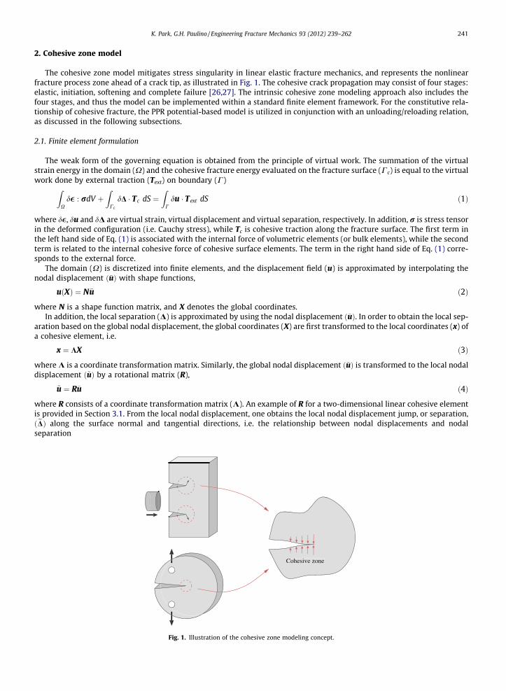
The present paper focuses on the implementation of the PPR potential-based cohesive zone model in ABAQUS as a UELsubroutine. The UEL subroutine is provided in Appendix for educational purposes. Notice that the finite element-basedintrinsic cohesive zone modeling approach is employed because it can be easily implemented in an existing standard finiteanalysis code. Furthermore, the PPR model can also be implemented in conjunction with other computational techniquessuch as extrinsic cohesive zone modeling [19,20], extended/generalized finite element method (XFEM/GFEM) [21,22], andembedded discontinuities [23–25]. However, as indicated above, the intrinsic model is the approach of choice in this paper.
The remainder of the paper is organized as follows. The formulation of cohesive elements and the PPR potential basedmodel are explained in the following section. Then, Section 3 presents the computational implementation of the PPR poten-tial-based model for a two-dimensional linear cohesive element. Section 4 investigates three examples: simple patch test,mixed-mode bending test and matrix/particle debonding. Finally, the paper is summarized in Section 5.
K. Park, G.H. Paulino / Engineering Fracture Mechanics 93 (2012) 239–262 241
2. Cohesive zone model
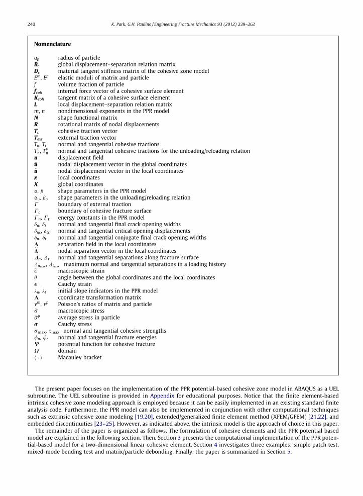
The cohesive zone model mitigates stress singularity in linear elastic fracture mechanics, and represents the nonlinearfracture process zone ahead of a crack tip, as illustrated in Fig. 1. The cohesive crack propagation may consist of four stages:elastic, initiation, softening and complete failure [26,27]. The intrinsic cohesive zone modeling approach also includes thefour stages, and thus the model can be implemented within a standard finite element framework. For the constitutive rela-tionship of cohesive fracture, the PPR potential-based model is utilized in conjunction with an unloading/reloading relation,as discussed in the following subsections.
2.1. Finite element formulation
The weak form of the governing equation is obtained from the principle of virtual work. The summation of the virtualstrain energy in the domain (X) and the cohesive fracture energy evaluated on the fracture surface (Cc) is equal to the virtualwork done by external traction (Text) on boundary (C)
ZXd� : rdV þ
ZCc
dD � Tc dS ¼Z
Cdu � Text dS ð1Þ
where d�, du and dD are virtual strain, virtual displacement and virtual separation, respectively. In addition, r is stress tensorin the deformed configuration (i.e. Cauchy stress), while Tc is cohesive traction along the fracture surface. The first term inthe left hand side of Eq. (1) is associated with the internal force of volumetric elements (or bulk elements), while the secondterm is related to the internal cohesive force of cohesive surface elements. The term in the right hand side of Eq. (1) corre-sponds to the external force.
The domain (X) is discretized into finite elements, and the displacement field (u) is approximated by interpolating thenodal displacement ð�uÞ with shape functions,
uðXÞ ¼ N�u ð2Þ
where N is a shape function matrix, and X denotes the global coordinates.In addition, the local separation (D) is approximated by using the nodal displacement ð�uÞ. In order to obtain the local sep-
aration based on the global nodal displacement, the global coordinates (X) are first transformed to the local coordinates (x) ofa cohesive element, i.e.
x ¼ KX ð3Þ
where K is a coordinate transformation matrix. Similarly, the global nodal displacement ð�uÞ is transformed to the local nodaldisplacement ð~uÞ by a rotational matrix (R),
~u ¼ R�u ð4Þ
where R consists of a coordinate transformation matrix (K). An example of R for a two-dimensional linear cohesive elementis provided in Section 3.1. From the local nodal displacement, one obtains the local nodal displacement jump, or separation,ðeDÞ along the surface normal and tangential directions, i.e. the relationship between nodal displacements and nodalseparation
Cohesive zone
Fig. 1. Illustration of the cohesive zone modeling concept.

242 K. Park, G.H. Paulino / Engineering Fracture Mechanics 93 (2012) 239–262
eD ¼ L~u ð5Þ
where L is a local displacement–separation relation matrix. Then, separation (D(x)) along a cohesive surface element is inter-polated from the nodal separation by using shape functions,
DðxÞ ¼ N eD: ð6Þ
Finally, the substitution of Eqs. (4) and (5) into Eq. (6) leads to the relationship between the local separation and the globalnodal displacement, i.e.
DðxÞ ¼ Bc �u ð7Þ
where Bc is a global displacement–separation relation matrix (i.e. Bc = NLR).Based on the approximated displacement field, the internal force vector (fcoh) of a cohesive surface element is given as
f coh ¼Z
Cc
BTc Tc dS: ð8Þ
The gradient of the internal cohesive force vector leads to the tangent matrix (Kcoh) of a cohesive surface element, i.e.
Kcoh ¼@f coh
@�u¼Z
Cc
BTc@Tc
@D@D@�u
dS ¼Z
Cc
BTc@Tc
@DBc dS: ð9Þ
Note that Tc and @Tc/@D are obtained from the PPR potential-based cohesive zone model, as presented in the following sub-section. In addition, the formulation is applicable for both two- and three-dimensional finite element implementations. Theimplementation procedure of a two-dimensional linear cohesive element is discussed in Section 3.
2.2. PPR Potential-based cohesive zone model
The cohesive traction–separation relationship is obtained from a potential-based cohesive zone model, so-called the PPRmodel [15,1]. The potential of cohesive fracture is given by
WðDn;DtÞ ¼minð/n;/tÞ þ Cn 1� Dn
dn
� �a maþ Dn
dn
� �m
þ h/n � /ti� �
Ct 1� jDtjdt
� �b nbþ jDt jdt
� �n
þ h/t � /ni" #
: ð10Þ
where h � i is the Macauley bracket, i.e.
hxi ¼0; ðx 6 0Þx; ðx > 0Þ:
�ð11Þ
Because of the nature of the potential, the derivatives of the PPR potential with respect to the normal and tangential sepa-rations lead to the normal and tangential cohesive tractions,
TnðDn;DtÞ ¼Cn
dnm 1� Dn
dn
� �a maþ Dn
dn
� �m�1
� a 1� Dn
dn
� �a�1 maþ Dn
dn
� �m" #
Ct 1� jDt jdt
� �b nbþ jDt j
dt
� �n
þ h/t � /ni" #
;
TtðDn;DtÞ ¼Ct
dtn 1� jDtj
dt
� �b nbþ jDtj
dt
� �n�1
� b 1� jDt jdt
� �b�1 nbþ jDt j
dt
� �n" #
Cn 1� Dn
dn
� �a maþ Dn
dn
� �m
þ h/n � /ti� �
Dt
jDt j; ð12Þ
respectively. Notice that the normal and tangential tractions satisfy basic symmetry and anti-symmetry requirements (withrespect to Dt), i.e. Tn(Dn, Dt) = Tn(Dn, �Dt) and Tt(Dn, Dt) = �Tt(Dn, �Dt). The value of Tt(Dn, Dt) at Dt = 0 exists in the limitsense. In addition, the PPR potential is defined within a cohesive interaction region. If separation is outside of the interactionregion, the cohesive traction is equal to zero.
The PPR potential-based model satisfies the following boundary conditions associated with cohesive fracture.
� The complete normal separation occurs (Tn = 0) when either normal or tangential separation reaches a certain lengthscale,
Tnðdn;DtÞ ¼ 0; TnðDn; �dtÞ ¼ 0; ð13Þ
where dn is a normal final crack opening width, and �dt is a tangential conjugate final crack opening width.� Similarly, the complete tangential separation occurs (Tt = 0) when either normal or tangential separation reaches a certain
length scale,

Fig. 2.(�dn , �dt).
K. Park, G.H. Paulino / Engineering Fracture Mechanics 93 (2012) 239–262 243
Ttð �dn;DtÞ ¼ 0; TtðDn; dtÞ ¼ 0: ð14Þ
where �dn is a normal conjugate final crack opening width, and dt is a tangential final crack opening width.� The area under the pure normal and tangential traction–separation curves provides the fracture energy in the normal (/n)
and tangential (/t) directions, respectively,
/n ¼Z dn
0TnðDn;0ÞdDn; /t ¼
Z dt
0Ttð0;DtÞdDt : ð15Þ
� The traction–separation curves reach a peak point at a critical crack opening width (dnc, dtc),
@Tn
@Dn
����Dn¼dnc
¼ 0;@Tt
@Dt
����Dt¼dtc
¼ 0: ð16Þ
Notice that the smaller value of the critical crack opening width results in the higher initial slope in the intrinsic traction–separation relationship. The limit of the critical crack opening widths in the PPR potential (dnc ? 0 and dtc ? 0) leads tothe traction–separation relationship for the extrinsic cohesive zone model.� The traction value at the critical separation corresponds to the cohesive strength (rmax, smax),
Tnðdnc;0Þ ¼ rmax; Ttð0; dtcÞ ¼ smax: ð17Þ
� The shape parameters (a, b) are introduced in order to represent various material softening responses. When the shapeparameters are smaller than two, the cohesive traction–separation relationship illustrates the concave shape (e.g. pla-teau-type). If a,b� 2, the relation is the convex shape, which can be applicable for typical quasi-brittle materials.
Based on proper boundary conditions, the characteristic parameters (dn, dt; Cn, Ct; m, n; a, b) in the PPR potential aredetermined. The energy constants Cn and Ct are related to the fracture energies (e.g. modes I and II). When the modes Iand II fracture energies are different, one obtains the energy constants
Cn ¼ ð�/nÞh/n�/t i/n�/t
am
� m
; Ct ¼ ð�/tÞh/t�/n i/t�/n
bn
� �n
for ð/n – /tÞ: ð18Þ
If the modes I and II fracture energies are the same, the energy constants are simplified as
Cn ¼ �/nam
� m
; Ct ¼bn
� �n
for ð/n ¼ /tÞ: ð19Þ
The exponents m and n are associated with the initial slope (i.e. artificial compliance),
m ¼ aða� 1Þk2n
ð1� ak2nÞ; n ¼ bðb� 1Þk2
t
ð1� bk2t Þ: ð20Þ
where kn and kt are initial slope indicators, which are the ratio of the critical crack opening width to the final crack openingwidth, i.e. (kn ¼ dnc=dn, kt ¼ dtc=dt). The normal final crack opening width (dn) is given as
dn ¼/n
rmaxaknð1� knÞa�1 a
mþ 1
� am
kn þ 1� m�1
ð21Þ
while the tangential final crack opening width (dt) is expressed as
dt ¼/t
smaxbktð1� ktÞb�1 b
nþ 1
� �bn
kt þ 1� �n�1
: ð22Þ
(a) (b)Description of each cohesive interaction (Tn, Tt) region defined by the final crack opening widths (dn, dt) and the conjugate final crack opening widths

244 K. Park, G.H. Paulino / Engineering Fracture Mechanics 93 (2012) 239–262
The cohesive interaction (or softening) region is defined in a rectangular domain, as shown in Fig. 2. The normal cohesiveinteraction region is determined by the first boundary condition (Eq. (13)), which provides two length scales: the normalfinal crack opening width (dn) and the conjugate tangential final crack opening width ð�dtÞ. When normal separation (Dn)is greater than dn or when the absolute of tangential separation is greater than �dt , the normal cohesive traction is set tobe zero. As a result, the normal softening region is a rectangular domain where 0 6Dn 6 dn and jDt j 6 �dt . The tangential con-jugate final crack opening width ðDt ¼ �dtÞ is the solution of the following nonlinear function,
Fig. 3.the nor
ftðDtÞ ¼ Ct 1� Dt
dt
� �b nbþ Dt
dt
� �n
þ h/t � /ni ¼ 0: ð23Þ
The solution ð�dtÞ is unique between 0 and dt. Similarly, the second boundary condition (Eq. (14)) defines the tangential cohe-sive interaction region, i.e. 0 6 Dn 6
�dn and jDtj 6 dt. The tangential cohesive traction is equal to zero when Dn P �dn orjDtjP dt. The normal conjugate final crack opening width ðDn ¼ �dnÞ is the solution of the nonlinear function,
fnðDnÞ ¼ Cn 1� Dn
dn
� �a maþ Dn
dn
� �m
þ h/n � /ti ¼ 0: ð24Þ
The solution ð�dnÞ is unique between 0 and dn.The normal cohesive interaction (Tn) is plotted in Fig. 3a with /n = 100 N/m, /t = 200 N/m, rmax = 40 MPa, smax = 30 MPa,
a = 5, b = 1.3, kn = 0.1, and kt = 0.2. When the tangential separation is equal to zero, the normal traction reaches the cohesivestrength at Dn = 0.1dn, then decreases to zero as Dn goes to dn, which corresponds to the mode I traction–separation relation-
(a)
(b)(a) Normal cohesive traction with respect to the increase of the tangential separation; (b) tangential cohesive traction with respect to the increase ofmal separation.

Fig. 4. PPR potential and its gradients for the intrinsic cohesive zone model with /n = 100 N/m, /t = 200 N/m, rmax = 40 MPa, smax = 30 MPa, a = 5, b = 1.3,kn = 0.1, and kt = 0.2.
K. Park, G.H. Paulino / Engineering Fracture Mechanics 93 (2012) 239–262 245
ship. The increase of the tangential separation from zero to the conjugate final crack opening width ð�dtÞ leads to the mono-tonic decrease of the normal cohesive interaction. When Dt is equal to �dt , the normal traction is equal to zero, i.e.TnðDn; �dtÞ ¼ 0. Thus, either Dn P dn or jDtjP �dt results in the complete normal failure condition. Fig. 3b describes the tangen-tial cohesive traction (Tt) with respect to the normal and tangential separations. The tangential traction reaches the peakpoint when the tangential separation corresponds to the critical separation (i.e. Dt = 0.2dt). The tangential traction monoton-ically decreases with respect to the increase of normal and tangential separations. The tangential traction becomes zerowhen the tangential separation is greater than or equal to the tangential final crack opening width (dt) or when the normalseparation is greater than or equal to the normal conjugate final crack opening width ð�dnÞ.
The PPR potential and its gradients are plotted in the positive softening region, shown in Fig. 4. The fracture parametersare the same as the parameters used in Fig. 3. The normal cohesive traction illustrates the convex shape while the tangentialcohesive traction describes the concave shape, as expected. In addition, the PPR model can be plotted by using a graphicaluser interface (GUI)1.
2.3. Unloading/reloading relationship
The dissipation of the fracture energy is associated with unloading and reloading. Thus, unloading/reloading relations areindependent of the PPR potential. For simplicity, the following unloading/reloading relationship [1] is provided
1 A so
TtnðDn;DtÞ ¼ TnðDnmax ;DtÞ
Dn
Dnmax
� �at
; Ttt ðDn;DtÞ ¼ TtðDn;DtmaxÞ
jDt jDtmax
� �bt Dt
jDt j; ð25Þ
where Dnmax is the maximum normal separation in a loading history, while Dtmax is the maximum absolute of tangential sep-aration in a loading history. The normal and tangential cohesive tractions of the unloading/reloading model are illustrated byblack solids in Fig. 5, as an example. Additionally, TnðDnmax ;DtÞ and TtðDn;Dtmax Þ, e.g. gray solids in Fig. 5, correspond to thecohesive tractions along the boundary between the softening condition and the unloading/reloading condition. Unload-ing/reloading shape parameters (at, bt) are introduced to describe various unloading/reloading relations. If at and bt areequal to one, the traction–separation relation is linear to the origin. When the shape parameter is smaller than 1, it demon-strates the concave shape. When at, bt > 1, it shows the convex shape.
The unloading/reloading condition is defined on the basis of the normal and tangential separation history. If the currentnormal separation is greater than Dnmax , the current separation state is normal softening (i.e. follows Eq. (12)). When
urce code written in MATLAB can be found in http://paulino.cee.illinois.edu/education_resources/PPR/GUI.rar

(a) (b)Fig. 6. Two-dimensional linear cohesive element and nodal displacements in (a) the global coordinates and (b) the local coordinates.
(a) (b)Fig. 5. Schematics of the unloading/reloading model: (a) normal interaction Tt
n
�and (b) tangential interaction Tt
t
�.
246 K. Park, G.H. Paulino / Engineering Fracture Mechanics 93 (2012) 239–262
0 < Dn < Dnmax , the current separation state is unloading/reloading, and thus the normal cohesive traction is obtained fromthe unloading/reloading relationship (i.e. Eq. (25)). Similarly, when the current tangential separation is greater than Dtmax , thecurrent separation state demonstrates tangential softening. If jDtj < Dtmax , the tangential cohesive traction is evaluated on thebasis of the unloading/reloading relationship. Then, the unloading/reloading condition for the normal cohesive traction isuncoupled with respect to the unloading/reloading condition for the tangential cohesive traction. Notice that it is possiblethat the normal cohesive traction demonstrates softening condition while the tangential traction displays unloading/reload-ing condition. Alternatively, one can employ other unloading/reloading relationships [28,1] in conjunction with the PPRpotential.
3. Computational implementation
A finite element-based intrinsic cohesive zone model is implemented as a UEL subroutine in ABAQUS. The subroutine fora two-dimensional linear cohesive element with the PPR potential-based model is provided in Appendix, as an example. Inthe subroutine, nodal coordinates (COORDS), nodal displacements in the global coordinates (U), and material parameters de-fined in an input file (PROPS) are available, while the right-hand-side vector (RHS) and the Jacobian matrix (AMATRX) of acohesive element need to be defined. In addition, state dependent variables (SVARS) can be updated at the end of a nonlineariteration. In the current implementation, nine input parameters are needed, i.e. normal fracture energy (/n), tangential frac-ture energy (/t), normal cohesive strength (rmax), tangential cohesive strength (smax), normal shape parameter (a), tangen-tial shape parameter (b), normal initial slope indicator (kn), tangential initial slope indicator (kt), and thickness of a cohesiveelement along the out-of-plane direction. The right-hand-side vector (RHS) is minus of the internal cohesive force vector, i.e.�fcoh, while the Jacobian matrix (AMATRX) corresponds to the tangent matrix of a cohesive element, i.e. Kcoh. In the statedependent variables (SVARS), the maximum normal and tangential separations at each integration point are stored. Thetwo-point Gauss quadrature rule is employed, and thus four state variables are stored at the end of nonlinear iteration. Inaddition, the unloading/reloading relation is assumed to be linear towards the origin. The two-dimensional linear cohesiveelement formulation is illustrated in the following subsection. The cohesive traction vector and the tangent matrix are eval-uated on the basis of the PPR potential-based model in conjunction with the cohesive interaction region.
3.1. Two-dimensional linear cohesive element
A two-dimensional linear cohesive element consists of four nodes, and each node has two degrees of freedom. Thus, acohesive element has eight global nodal displacement quantities (�u1, �u2, �u3, �u4, �u5, �u6, �u7, �u8), as shown in Fig. 6a. These globalquantities are transformed into local nodal displacement quantities (~u1, ~u2, ~u3, ~u4, ~u5, ~u6, ~u7, ~u8) by the rotational matrix, R

K. Park, G.H. Paulino / Engineering Fracture Mechanics 93 (2012) 239–262 247
R ¼
K 0 0 00 K 0 00 0 K 00 0 0 K
2666437775 ð26Þ
where the two-dimensional transformation matrix (K) is given as:
K ¼cos h sin h
� sin h cos h
� �: ð27Þ
Note that h is the angle between the global coordinates and the local coordinates. In the current computational implemen-tation, the order of the nodes of a cohesive element is counter clockwise, and the node numbering starts from the lower leftnode of a cohesive element in the transformed configuration, as shown in Fig. 6b.
Then, the nodal normal separation and tangential separation at the end of a cohesive element (eD1, eD2, eD3, eD4) can be ob-tained from the local nodal displacement as follows,
eD1 ¼ ~u7 � ~u1; eD2 ¼ ~u8 � ~u2; eD3 ¼ ~u5 � ~u3; eD4 ¼ ~u6 � ~u4: ð28ÞBased on the above relations, the local displacement–separation relation matrix (L) is given as
L ¼
�1 0 0 0 0 0 1 00 �1 0 0 0 0 0 10 0 �1 0 1 0 0 00 0 0 �1 0 1 0 0
2666437775: ð29Þ
The separation along the cohesive element is obtained from the nodal separation quantities in conjunction with the shapefunctional matrix (N),
N ¼N1 0 N2 00 N1 0 N2
� �ð30Þ
where the linear shape functions in the natural coordinate (n) are given as
N1 ¼1� n
2; N2 ¼
1þ n2
: ð31Þ
From Eqs. (26)–(30), the global displacement–separation relation matrix (Bc) is expressed as
Bc ¼�CN1 �SN1 �CN2 �SN2 CN2 SN2 CN1 SN1
SN1 �CN1 SN2 �CN2 �SN2 CN2 �SN1 CN1
� �ð32Þ
where C and S denote cosh and sinh, respectively. Finally, the internal cohesive force vector (Eq. (8)) and the tangent matrix(Eq. (9)) are computed by using a numerical integration scheme (e.g. Gauss quadrature).
3.2. Determination of cohesive interaction region
The cohesive interaction (softening) region is associated with the length scales: the final crack opening widths (dn, dt) andthe conjugate final crack opening widths (�dn, �dt). The softening region of the normal cohesive traction is defined as0 6Dn 6 dn and ��dt 6 Dt 6
�dt while the softening region of the tangential cohesive traction is defined as 0 6 Dn 6�dn and
�dt 6Dt 6 dt. For the intrinsic cohesive zone model, the normal and tangential final crack opening widths are determinedby the closed form (Eqs. (21) and (22)), while the conjugate final crack opening widths are calculated by solving the nonlin-ear equations (Eqs. (23) and (24)). The nonlinear equations can be solved by a root-finding algorithm, such as the Bisectionmethod or the Newton–Raphson method.
Alternatively, the softening region can be defined without solving the nonlinear equation. The necessary and sufficientconditions of ð��dt 6 Dt 6
�dtÞ, associated with the normal softening region, are ((�dt 6 Dt 6 dt) & (Tn(Dn, Dt) P 0)). This is be-cause the tangential conjugate final crack opening width ð�dtÞ is unique between zero and the tangential final crack openingwidth (dt) and because the normal cohesive traction is always positive within the normal softening region. Similarly, one canreplace ð0 6 Dn 6
�dnÞ by ((0 6 Dn 6 dn) & (Tt(Dn, Dt) P 0)) because �dn is unique between 0 and dn, and because the tangentialtraction is positive within the tangential softening region. Notice that this alternative approach is employed in the UEL sub-routine provided in Appendix.
3.3. Cohesive traction vector and tangent matrix
The cohesive traction vector and the material tangent stiffness matrix are evaluated by accounting for four cases: soften-ing, unloading/reloading, contact and complete failure conditions. Algorithm 1 outlines the evaluation of the cohesive trac-tion vector (Tc) and tangent matrix (Dc) with respect to the four cases. Notice that the normal and tangential cohesiveinteractions are evaluated independently.

248 K. Park, G.H. Paulino / Engineering Fracture Mechanics 93 (2012) 239–262
Algorithm 1. Evaluation of the cohesive traction vector and tangent matrix based on the four conditions: softening,unloading/reloading, contact and complete failure.
// Normal cohesive interaction:if (Dn 6 0) then {Contact}
Tn = DnnDn, Dnn = ap, Dnt = 0
else if (0 6 Dn 6 dn and jDt j 6 �dt and Dn P Dnmax Þ then {Softening}
Tn ¼ @WðDn ;DtÞ@Dn
; Dnt ¼ @2WðDn ;DtÞ@D2
n; Dnt ¼ @2WðDn ;DtÞ
@Dn@Dt
else if (0 6 Dn 6 dn and jDt j 6 �dt and Dn < Dnmax ) then {Unloading/reloading}
Tn ¼ TtnðDn;DtÞ; Dnn ¼ @Tt
nðDn ;DtÞ@Dn
; Dnt ¼ @TtnðDn ;DtÞ@Dt
else if (Dn > dn or jDt j > �dt) then {Complete failure}Tn = 0, Dnn = 0, Dnt = 0
end if
// Tangential cohesive interaction:if (Dn 6 0) then {Contact}
Dn = 0end if
if (0 6 Dn 6�dn and jDtj 6 dt and jDt jP Dtmax ) then {Softening}
Tt ¼ @WðDn ;DtÞ@Dt
; Dtn ¼ @2WðDn ;DtÞ@DtDn
; Dtt ¼ @2WðDn ;DtÞ@D2
t
else if (0 6 Dn 6�dn and jDtj 6 dt and jDtj < Dtmax ) then {Unloading/reloading}
Tt ¼ Ttt ðDn;DtÞ; Dtn ¼ @Tt
t ðDn ;DtÞ@Dn
; Dtt ¼ @Ttt ðDn ;DtÞ@Dt
else if ((Dn > �dn) or (jDtj > dt)) then {Complete failure}Tt = 0, Dtn = 0, Dtt = 0
end if
First, when separations are within the cohesive interaction region and when the current separation is greater than themaximum separation in a loading history, the current state of separation follows the softening condition. Thus, the constitu-tive relationship is derived from the PPR potential. If both normal and tangential separations are in the softening condition,the cohesive tractions are evaluated by taking the derivatives of the PPR potential,
TcðDn;DtÞ ¼@W=@Dt
@W=@Dn
� �¼
TtðDn;DtÞTnðDn;DtÞ
� �; ð33Þ
as shown in Eq. (12). The second derivatives of the PPR potential lead to the material tangent stiffness matrix,
DcðDn;DtÞ ¼Dtt Dtn
Dnt Dnn
� �¼
@2W=@D2t @2W=@Dt@Dn
@2W=@Dn@Dt @2W=@D2n
" #; ð34Þ
where the components of the matrix are given as
Dnn ¼Cn
d2n
ðm2 �mÞ 1� Dn
dn
� �a maþ Dn
dn
� �m�2
þ ða2 � aÞ 1� Dn
dn
� �a�2 maþ Dn
dn
� �m"
�2am 1� Dn
dn
� �a�1 maþ Dn
dn
� �m�1#
Ct 1� jDt jdt
� �b nbþ jDt j
dt
� �n
þ h/t � /ni" #
;
Dnt ¼CnCt
dndtm 1� Dn
dn
� �a maþ Dn
dn
� �m�1
� a 1� Dn
dn
� �a�1 maþ Dn
dn
� �m" #
n 1� jDtjdt
� �b nbþ jDtj
dt
� �n�1
� b 1� jDt jdt
� �b�1 nbþ jDt j
dt
� �n" #
Dt
jDtj;
Dtn ¼ Dnt;
Dtt ¼Ct
d2t
ðn2 � nÞ 1� jDt jdt
� �b nbþ jDtj
dt
� �n�2
þ ðb2 � bÞ 1� jDt jdt
� �b�2 nbþ jDt j
dt
� �n"
�2bn 1� jDtjdt
� �b�1 nbþ jDtj
dt
� �n�1#
Cn 1� Dn
dn
� �a maþ Dn
dn
� �m
þ h/n � /ti� �
: ð35Þ
In this case, as expected, one obtains the symmetric tangent stiffness matrix.
K. Park, G.H. Paulino / Engineering Fracture Mechanics 93 (2012) 239–262 249
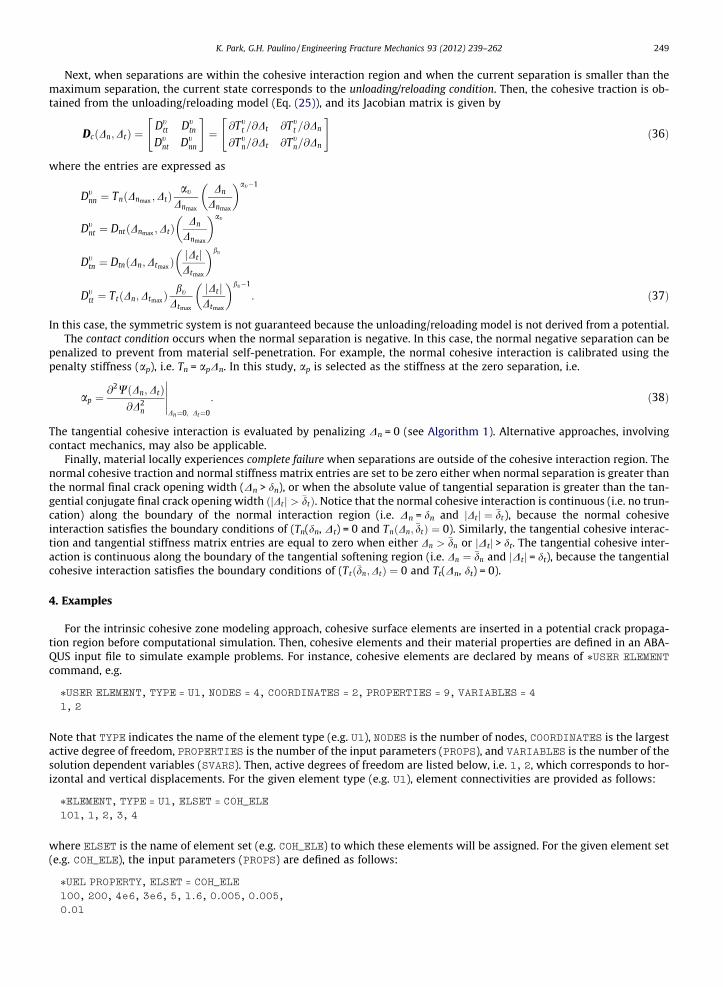
Next, when separations are within the cohesive interaction region and when the current separation is smaller than themaximum separation, the current state corresponds to the unloading/reloading condition. Then, the cohesive traction is ob-tained from the unloading/reloading model (Eq. (25)), and its Jacobian matrix is given by
DcðDn;DtÞ ¼Dt
tt Dttn
Dtnt Dt
nn
" #¼
@Ttt =@Dt @Tt
t =@Dn
@Ttn=@Dt @Tt
n=@Dn
" #ð36Þ
where the entries are expressed as
Dtnn ¼ TnðDnmax ;DtÞ
at
Dnmax
Dn
Dnmax
� �at�1
Dtnt ¼ DntðDnmax ;DtÞ
Dn
Dnmax
� �at
Dttn ¼ DtnðDn;DtmaxÞ
jDtjDtmax
� �bt
Dttt ¼ TtðDn;DtmaxÞ
bt
Dtmax
jDt jDtmax
� �bt�1
: ð37Þ
In this case, the symmetric system is not guaranteed because the unloading/reloading model is not derived from a potential.The contact condition occurs when the normal separation is negative. In this case, the normal negative separation can be
penalized to prevent from material self-penetration. For example, the normal cohesive interaction is calibrated using thepenalty stiffness (ap), i.e. Tn = apDn. In this study, ap is selected as the stiffness at the zero separation, i.e.
ap ¼@2WðDn;DtÞ
@D2n
�����Dn¼0; Dt¼0
: ð38Þ
The tangential cohesive interaction is evaluated by penalizing Dn = 0 (see Algorithm 1). Alternative approaches, involvingcontact mechanics, may also be applicable.
Finally, material locally experiences complete failure when separations are outside of the cohesive interaction region. Thenormal cohesive traction and normal stiffness matrix entries are set to be zero either when normal separation is greater thanthe normal final crack opening width (Dn > dn), or when the absolute value of tangential separation is greater than the tan-gential conjugate final crack opening width ðjDt j > �dtÞ. Notice that the normal cohesive interaction is continuous (i.e. no trun-cation) along the boundary of the normal interaction region (i.e. Dn = dn and jDtj ¼ �dt), because the normal cohesiveinteraction satisfies the boundary conditions of (Tn(dn, Dt) = 0 and TnðDn; �dtÞ ¼ 0). Similarly, the tangential cohesive interac-tion and tangential stiffness matrix entries are equal to zero when either Dn > �dn or jDtj > dt. The tangential cohesive inter-action is continuous along the boundary of the tangential softening region (i.e. Dn ¼ �dn and jDtj = dt), because the tangentialcohesive interaction satisfies the boundary conditions of (Ttð�dn;DtÞ ¼ 0 and Tt(Dn, dt) = 0).
4. Examples
For the intrinsic cohesive zone modeling approach, cohesive surface elements are inserted in a potential crack propaga-tion region before computational simulation. Then, cohesive elements and their material properties are defined in an ABA-QUS input file to simulate example problems. For instance, cohesive elements are declared by means of ⁄USER ELEMENT
command, e.g.
⁄USER ELEMENT, TYPE = U1, NODES = 4, COORDINATES = 2, PROPERTIES = 9, VARIABLES = 4
1, 2
Note that TYPE indicates the name of the element type (e.g. U1), NODES is the number of nodes, COORDINATES is the largestactive degree of freedom, PROPERTIES is the number of the input parameters (PROPS), and VARIABLES is the number of thesolution dependent variables (SVARS). Then, active degrees of freedom are listed below, i.e. 1, 2, which corresponds to hor-izontal and vertical displacements. For the given element type (e.g. U1), element connectivities are provided as follows:
⁄ELEMENT, TYPE = U1, ELSET = COH_ELE101, 1, 2, 3, 4
where ELSET is the name of element set (e.g. COH_ELE) to which these elements will be assigned. For the given element set(e.g. COH_ELE), the input parameters (PROPS) are defined as follows:
⁄UEL PROPERTY, ELSET = COH_ELE100, 200, 4e6, 3e6, 5, 1.6, 0.005, 0.005,
0.01
where input parameters are provided as an example. Nine parameters are required, and listed as the following orders: /n, /t,r , s , a, b, k , k , and thickness along the out-of-plane direction. After generating an input file, one can execute an anal-
max max n tysis in conjunction with the UEL subroutine through the following command, i.e.
abaqus job = input_file_name user = UEL_file_name
250 K. Park, G.H. Paulino / Engineering Fracture Mechanics 93 (2012) 239–262
More detailed information associated with an ABAQUS input file and its execution can be found in the ABAQUS/standarduser’s manual [16].
In order to verify the UEL subroutine, three computational examples are provided: patch test, mixed-mode bending test,and matrix/particle debonding. For patch tests, simple mode-I and mode-II tests are simulated, which display constant stressstate within continuum (or bulk) elements. In addition, mixed-mode bending and matrix/particle debonding examples areinvestigated by comparing computational results to analytical solutions.
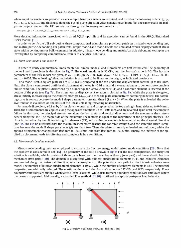
4.1. Patch test: mode-I and mode-II
In order to verify computational implementation, simple modes I and II problems are first introduced. The geometry ofmodes I and II problems is described in Fig. 7. The elastic modulus is 32 GPa, and the Poisson’s ratio is 0.2. The fractureparameters of the PPR model are given as /n = 100 N/m, /t = 200 N/m, rmax = 4 MPa, smax = 3 MPa, a = 5, b = 1.6,kn = 0.005,and kt = 0.005. The unloading/reloading relation is assumed to be linear to the origin, as indicated previously.
For a mode I test, a square plate (0.1 m � 0.1 m) is elongated at the top under the displacement control up to 0.03 mm.Next, the plate is compressed until the displacement at the top is �0.01 mm, and is elongated again to demonstrate completefailure condition. The plate is discretized by a bilinear quadrilateral element (Q4), and a cohesive element is inserted at thebottom of the plate (see Fig. 7a). The stress versus displacement relation is plotted in Fig. 8a. While the plate is elongated,stress initially increases up to the cohesive strength (rmax), and then the plate demonstrates softening behavior. The soften-ing curve is convex because the mode I shape parameter is greater than 2 (i.e. a = 5). When the plate is unloaded, the cohe-sive traction is evaluated on the basis of the linear unloading/reloading relationship.
For a mode II problem, a 0.1 m by 0.1 m plate is elongated and compressed at the top and right hand sides up to 0.04 mm.Then, the displacements are applied along the opposite directions up to�0.05 mm, and are reversed again until the completefailure. In this case, the principal stresses are along the horizontal and vertical directions, and the maximum shear stressoccurs along the 45�. The magnitude of the maximum shear stress is equal to the magnitude of the principal stresses. Theplate is discretized by two linear triangular elements (T3), and a cohesive element is inserted along the diagonal direction(see Fig. 7b). Fig. 8b illustrates that the maximum shear stress reaches the cohesive strength, and the softening curve is con-cave because the mode II shape parameter (b) less than two. Then, the plate is linearly unloaded and reloaded, while theapplied displacement changes from 0.04 mm to �0.04 mm, and from 0.05 mm to �0.05 mm. Finally, the increase of the ap-plied displacement leads to softening and complete failure conditions.
4.2. Mixed-mode bending analysis
Mixed-mode bending tests are employed to estimate the fracture energy under mixed mode conditions [29]. Note thatthe problem is considered in Ref [15]. The geometry of the test is shown in Fig. 9. For the test configuration, the analyticalsolution is available, which consists of three parts based on the linear beam theory (one part) and linear elastic fracturemechanics (two parts) [30]. The domain is discretized with bilinear quadrilateral elements (Q4), and cohesive elementsare inserted along the horizontal direction, which corresponds to the potential crack path, i.e. the intrinsic cohesive zonemodel. The number of bilinear quadrilateral elements is 19,570 while the number of cohesive elements is 683. The materialproperties are arbitrarily selected. The elastic modulus and the Poisson’s ratio are 122 GPa and 0.25, respectively. Forceboundary conditions are applied where a rigid lever is located, while displacement boundary conditions are employed wherethe beam is supported. Additionally, a modified Riks method [31,16] is utilized to capture post-peak load behavior.
(a) (b)Fig. 7. Geometry of (a) mode I test, and (b) mode II test.

Fig. 9. Geometry of the mixed-mode bending test.
(a)
(b)Fig. 8. Computational results: (a) mode I test, and (b) mode II test.
K. Park, G.H. Paulino / Engineering Fracture Mechanics 93 (2012) 239–262 251
In this study, two cases are tested. One is that the mode I fracture energy is the same as the mode II fracture energy (e.g./n = /t = 500 N/m). The other is that the mode I fracture energy is different from the mode II fracture energy (e.g. /n = 500 N/m,/t = 1000 N/m). The shape parameter (a,b) is 3, and the initial slope indicator (kn,kt) is 0.02 for both cases. For the same fractureenergy, the computational results obtained with various cohesive strengths (rmax, smax) are illustrated in Fig. 10a. The increase

(a)
(b)Fig. 10. Comparison between the analytical solutions and the computational results: (a) /n = /t = 500 N/m, and (b) /n = 500 N/m, /t = 1000 N/m.
Fig. 11. Unit cell with a cylindrical particle under equi-biaxial tension stress state.
252 K. Park, G.H. Paulino / Engineering Fracture Mechanics 93 (2012) 239–262

K. Park, G.H. Paulino / Engineering Fracture Mechanics 93 (2012) 239–262 253
of the cohesive strength leads to more brittle failure behavior, and thus demonstrates the convergence to the analytical solutions.For the case of different fracture energies, the normal cohesive strength is fixed as 20 MPa while the tangential cohesive strengthchanges from 100 MPa to 500 MPa. Similarly, the computational results converges to the analytical solutions while the tangentialcohesive strength (smax) increases, as shown in Fig. 10b.
4.3. Multiscale analysis through matrix/particle debonding
Matrix/particle debonding process is analyzed, and computational results are compared with the results obtained from amicro-mechanics approach. In this study, one assumes that all particles are isotropic, and have the same elastic modulus andparticle size. The shape of a unit cell are a regular hexahedron with a cylindrical particle, as illustrated in Fig. 11. Boundaryconditions of a unit cell are idealized as the equibiaxial tension under plane strain condition. The particle volume fraction (f)is associated with the unit cell size and the radius of particle (ap). Based on the extended Mori–Tanaka method [32,13], themacroscopic strain ð��Þ and the macroscopic stress ð�rÞ are given as:
�� ¼ ð1þ mmÞð1� 2mmÞEm �rþ f
ð1þ mpÞð1� 2mpÞEp � ð1þ mmÞð1� 2mmÞ
Em
� ��rp þ Dn
ap
� �ð39Þ
Number of nodes: 7128Number of volumetric elements (Q4): 6826Number of cohesive elements: 200
(a)
(b)Fig. 12. (a) Finite element mesh of the unit cell, and (b) Mises stress distribution for the case of rmax = 10 MPa.

Fig. 13. Macroscopic stress versus strain relations with respect to the change of the cohesive strength.
254 K. Park, G.H. Paulino / Engineering Fracture Mechanics 93 (2012) 239–262
and
�r ¼ ð1� f ÞEm
2ð1� mmÞð1þ mmÞð1þ mpÞð1� 2mpÞ
Ep þ 1þ mm
Em
� ��rp þ Dn
ap
� �þ f �rp; ð40Þ
where Em and Ep are elastic modulus of matrix and particle, and mm and mp are Poisson’s ratio of matrix and particle, respec-tively. In addition, the average stress in the particle ð�rpÞ is uniform, and thus equals to the normal cohesive traction at theparticle/matrix interface (Tn), which is related to the normal separation (Dn) in the PPR model.
The particle size (ap) is 2 cm, and the volume fraction (f) of the particle is 0.6. A quarter of the unit cell is analyzed becauseof symmetry along the horizontal and vertical directions. The corresponding finite element mesh is illustrated in Fig. 12a,and cohesive elements are inserted along the matrix/particle interface. The elastic modulus of particle (Ep) is 40 GPa whilethe modulus of matrix (Em) is 20 GPa. Both particle and matrix have the same Poisson’s ratio, i.e. mp = mm = 0.25. The mode Ifracture parameters are assumed to be the same as the mode II fracture parameters. The fracture energy is 100 N/m, theshape parameter is 3, and the initial slope indicator is 0.001. Three cases are tested by changing the cohesive strength,i.e. rmax = 10 MPa, 8 MPa and 6 MPa. Fig. 12b illustrates the stress distribution after the peak load for the case of rmax = 10 M-Pa. In addition, the macroscopic stress versus strain relations obtained from the finite element computation are comparedwith the results from the extended Mori–Tanaka method, as shown in Fig. 13. The increase of the cohesive strength leadsto more brittle failure behavior, and increases the peak stress of the averaged macroscopic stress.
5. Concluding remarks
This paper presents the implementation of the PPR potential-based model in ABAQUS using a UEL subroutine. The imple-mentation is based on the intrinsic cohesive zone modeling approach, which includes the initial elastic range in the traction–separation relation. The input file format is provided for educational purposes. The UEL subroutine is provided in Appendix.In the PPR potential-based model, the cohesive traction and its tangent matrix are evaluated by considering four conditions:softening, unloading/reloading, contact and complete failure. The cohesive traction is obtained from the PPR potential for thesoftening condition, while it is computed from the unloading/reloading model for the unloading/reloading condition. For thecontact condition, a penalty stiffness is introduced along the normal direction to prevent material interpenetration. The com-plete failure condition is associated with the cohesive interaction region. The interaction region is defined within the finalcrack opening width (dn, dt) and the conjugate final crack opening width (�dn, �dt) space. Note that dn and dt are explicitly com-puted, while �dn and �dt can be computed by solving a nonlinear equation. Alternatively, rather than solving a nonlinear equa-tion, the interaction region can be determined by checking the sign of the cohesive traction. Finally, three computationalexamples are investigated to verify the present formulation: patch test, mixed-mode bending test, and matrix/particle deb-onding. We have shown how to implement the PPR model in ABAQUS/Standard, which includes an implicit solution tech-nique. We close this paper with a challenge for students interested in this line of research. We suggest that thosestudents implement the PPR model in ABAQUS/Explicit and explore simulations of cohesive elasto-dynamic fracture suchas those presented in reference [33].
Acknowledgements
Dr. Park acknowledges support from the National Research Foundation (NRF) of Korea through Grant Young Researchers#2011-0013393. The information presented in this paper is the sole opinion of the authors and does not necessarily reflectthe views of the sponsoring agency.

K. Park, G.H. Paulino / Engineering Fracture Mechanics 93 (2012) 239–262 255
Appendix A2
2 The source code provided in this appendix can be downloaded from the urlhttp://paulino.cee.illinois.edu or http://k-park.yonsei.ac.kr

256 K. Park, G.H. Paulino / Engineering Fracture Mechanics 93 (2012) 239–262

K. Park, G.H. Paulino / Engineering Fracture Mechanics 93 (2012) 239–262 257

258 K. Park, G.H. Paulino / Engineering Fracture Mechanics 93 (2012) 239–262
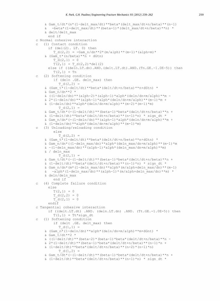
K. Park, G.H. Paulino / Engineering Fracture Mechanics 93 (2012) 239–262 259

260 K. Park, G.H. Paulino / Engineering Fracture Mechanics 93 (2012) 239–262

K. Park, G.H. Paulino / Engineering Fracture Mechanics 93 (2012) 239–262 261

262 K. Park, G.H. Paulino / Engineering Fracture Mechanics 93 (2012) 239–262
References
[1] Park K. Potential-based fracture mechanics using cohesive zone and virtual internal bond modeling. PhD Thesis, University of Illinois at Urbana-Champaign; 2009.
[2] Anderson TL. Fracture mechanics: fundamentals and applications. Boca Raton: CRC Press; 1995.[3] Barenblatt GI. The formation of equilibrium cracks during brittle fracture: general ideas and hypotheses, axially symmetric cracks. Appl Math Mech
1959;23(3):622–36.[4] Dugdale DS. Yielding of steel sheets containing slits. J Mech Phys Solids 1960;8(2):100–4.[5] Hillerborg A, Modeer M, Petersson PE. Analysis of crack formation and crack growth in concrete by means of fracture mechanics and finite elements.
Cement Concr Res 1976;6(6):773–81.[6] Boone TJ, Wawrzynek PA, Ingraffea AR. Simulation of the fracture process in rock with application to hydrofracturing. Int J Rock Mech Min Sci
1986;23(3):255–65.[7] Bazant ZP, Planas J. Fracture and size effect in concrete and other quasibrittle materials. Boca Raton: CRC Press; 1998.[8] Park K, Paulino GH, Roesler JR. Determination of the kink point in the bilinear softening model for concrete. Engng Fract Mech 2008;75(13):3806–18.[9] Ingraffea AR, Gerstle WH, Gergely P, Saouma V. Fracture mechanics of bond in reinforced concrete. J Struct Engng 1984;110(4):871–90.
[10] Xu C, Siegmund T, Ramani K. Rate-dependent crack growth in adhesives: I. Modeling approach. Int J Adhes Adhes 2003;23(1):9–13.[11] Matous K, Kulkarni MG, Geubelle PH. Multiscale cohesive failure modeling of heterogeneous adhesives. J Mech Phys Solids 2008;56(4):1511–33.[12] Xu XP, Needleman A. Void nucleation by inclusion debonding in a crystal matrix. Modell Simul Mater Sci Engng 1993;1(2):111–32.[13] Ngo D, Park K, Paulino GH, Huang Y. On the constitutive relation of materials with microstructure using a potential-based cohesive model for interface
interaction. Engng Fract Mech 2010;77(7):1153–74.[14] Needleman A, Borders TL, Brinson L, Flores VM, Schadler LS. Effect of an interphase region on debonding of a CNT reinforced polymer composite.
Compos Sci Technol 2010;70(15):2207–15.[15] Park K, Paulino GH, Roesler JR. A unified potential-based cohesive model of mixed-mode fracture. J Mech Phys Solids 2009;57(6):891–908.[16] ABAQUS. Version 6.2. H.K.S. Pawtucket: Hibbitt, Karlsson & Sorensen; 2002.[17] Sigmund O. A 99 line topology optimization code written in Matlab. Struct Multidisc Optimiz 2001;21(2):120–7.[18] Giner E, Sukumar N, Tarancon JE, Fuenmayor FJ. An ABAQUS implementation of the extended finite element method. Engng Fract Mech
2009;76(3):347–68.[19] Ortiz M, Pandolfi A. Finite-deformation irreversible cohesive elements for three-dimensional crack-propagation analysis. Int J Numer Meth Engng
1999;44(9):1267–82.[20] Zhang Z, Paulino GH, Celes W. Extrinsic cohesive modelling of dynamic fracture and microbranching instability in brittle materials. Int J Numer Meth
Engng 2007;72(8):893–923.[21] Wells GN, Sluys LJ. A new method for modelling cohesive cracks using finite elements. Int J Numer Meth Engng 2001;50(12):2667–82.[22] Moes N, Belytschko T. Extended finite element method for cohesive crack growth. Engng Fract Mech 2002;69(7):813–33.[23] Simo JC, Oliver J, Armero F. An analysis of strong discontinuities induced by strain-softening in rate-independent inelastic solids. Comput Mech
1993;12(5):277–96.[24] Oliver J, Huespe AE, Pulido MDG, Chaves E. From continuum mechanics to fracture mechanics: the strong discontinuity approach. Engng Fract Mech
2002;69(2):113–36.[25] Linder C, Armero F. Finite elements with embedded strong discontinuities for the modeling of failure in solids. Int J Numer Meth Engng
2007;72(12):1391–433.[26] Klein PA, Foulk JW, Chen EP, Wimmer SA, Gao HJ. Physics-based modeling of brittle fracture: cohesive formulations and the application of meshfree
methods. Theor Appl Fract Mech 2001;37(1–3):99–166.[27] Roesler J, Paulino GH, Park K, Gaedicke C. Concrete fracture prediction using bilinear softening. Cem Concr Compos 2007;29(4):300–12.[28] Roe KL, Siegmund T. An irreversible cohesive zone model for interface fatigue crack growth simulation. Engng Fract Mech 2003;70(2):209–32.[29] Reeder JR, Crews Jr JH. Mixed-mode bending method for delamination testing. AIAA J 1990;28(7):1270–6.[30] Mi Y, Crisfield MA, Davies GAO, Hellweg HB. Progressive delamination using interface elements. J Compos Mater 1998;32(14):1246–72.[31] Crisfield MA. A fast incremental/iterative solution procedure that handles snap-through. Comput Struct 1981;13(1-3):55–62.[32] Tan H, Liu C, Huang Y, Geubelle PH. The cohesive law for the particle/matrix interfaces in high explosives. J Mech Phys Solids 2005;53(8):1892–917.[33] Zhang Z, Paulino GH. Cohesive zone modeling of dynamic failure in homogeneous and functionally graded materials. Int J Plast 2005;21(6):1195–254.