Engineering, Economic, and EnvironmentalElectricity Simulation Tool

E4ST 1.0b2User’s Manual

primary developersBiao Mao

Carlos E. Murillo-SanchezDaniel L. ShawhanRay D. Zimmerman

other contributorsCharles M. MarquetDoug Mitarotonda

Yingying QiWilliam D. SchulzeRichard E. Schuler

Di ShiJohn Tabor

Daniel J. TylavskyJubo YanYujia Zhu

February 18, 2016

© 2010, 2011, 2012, 2013, 2014, 2015, 2016 Power Systems Engineering Research Center (PSerc)

All Rights Reserved

Contents

1 Introduction 31.1 Background . . . . . . . . . . . . . . . . . . . . . . . . . . . . . . . . 31.2 License and Terms of Use . . . . . . . . . . . . . . . . . . . . . . . . 41.3 Citing E4ST . . . . . . . . . . . . . . . . . . . . . . . . . . . . . . . . 5

2 Getting Started 62.1 System Requirements . . . . . . . . . . . . . . . . . . . . . . . . . . . 62.2 Installation . . . . . . . . . . . . . . . . . . . . . . . . . . . . . . . . 62.3 Running a Simulation . . . . . . . . . . . . . . . . . . . . . . . . . . . 7

2.3.1 Preparing Input Data . . . . . . . . . . . . . . . . . . . . . . . 72.3.2 Solving the Case . . . . . . . . . . . . . . . . . . . . . . . . . 72.3.3 Accessing the Results . . . . . . . . . . . . . . . . . . . . . . . 82.3.4 Setting Options . . . . . . . . . . . . . . . . . . . . . . . . . . 9

2.4 Documentation . . . . . . . . . . . . . . . . . . . . . . . . . . . . . . 9

3 Problem Formulation 103.1 Nomenclature . . . . . . . . . . . . . . . . . . . . . . . . . . . . . . . 103.2 Objective function . . . . . . . . . . . . . . . . . . . . . . . . . . . . 123.3 Constraints . . . . . . . . . . . . . . . . . . . . . . . . . . . . . . . . 13

4 Acknowledgments 15

Appendix A E4ST Files and Functions 16

Appendix B Data Structures and Definitions 17B.1 Data Structure of CaseInfo . . . . . . . . . . . . . . . . . . . . . . . 17B.2 Data Structure of PolicyInfo . . . . . . . . . . . . . . . . . . . . . . . 19B.3 Data Structure of E4STResult . . . . . . . . . . . . . . . . . . . . . . 19

References 21

List of Tables

A-1 E4ST Files, Classes and Functions . . . . . . . . . . . . . . . . . . . . 16B-1 Data Structure of E4STResult . . . . . . . . . . . . . . . . . . . . . . 20

2

1 Introduction

1.1 Background

The Engineering, Economic, and Environmental Electricity Simulation Tool [1, 2],or E4ST (pronounced “east”), was developed by faculty and research staff at Cornell,Rensselaer Polytechnic Institute, Arizona State Universities and at Resources for theFuture, with support from the U. S. Department of Energy’s Certs program as wellas the Power Systems Engineering Research Center (PSerc). The code itself wasdeveloped primarily by Biao Mao, Carlos Murillo-Sanchez and Ray Zimmerman withcontributions by others, but the E4ST project as a whole was a much larger enterprisewith major contributions and efforts by a larger group.

E4ST is built on top of Matpower1, a package of Matlab® M-files for solvingpower flow and optimal power flow problems [3, 4] and is available openly, withoutcharge from the E4ST home page:

http://www.e4st.com/

It consists of a set of software toolboxes that can be used to estimate presentand future operating and investment states of an electric power system, includinggenerator dispatches, generator entry and retirement, locational prices, fixed and fuelcosts, air emissions, and environmental damages. The E4ST software toolboxes canbe used with suitable data from any part of the world.

E4ST can be applied to detailed system models. Algorithms are included thatsimulate the economic operation of the power grid, in response to the model-user’sprojections of economic factors (e.g. fuel prices), government incentives or envi-ronmental regulations. Simultaneously, the algorithms project and implement theeconomical investment and retirement of generation over time, by location. Thealgorithms are designed to maintain the redundancy necessary for service reliability.

E4ST is useful for both energy and environmental-policy planning purposes. Itaccounts for short and long-term feedbacks between energy and environmental poli-cies. It can be used to project the operation and evolution of the power system underany combination of prices, demand patterns, and policies specified by the user. Itcan calculate the net benefits of any policy simulated, and disaggregate them intothe benefits or costs for customers, generation owners, the system operator, the gov-ernment, public health, and the environment.

In addition, E4ST can be used as a transmission planning tool to explore theconsequences of network changes. The existing electric transmission system is fixed

1See http://www.pserc.cornell.edu/matpower/ for more information on Matpower.

3

throughout these simulations, and only the generator dispatches and customer loadsrespond endogenously, but the user can change the transmission network and re-run the simulation to calculate the effects of the change, potentially repeating thisthousands of times to test many different transmission system investment scenarios.

1.2 License and Terms of Use

The code in E4ST is distributed under the 3-clause BSD license [5]. The full text ofthe license can be found in the LICENSE file at the top level of the distribution andreads as follows:

Copyright (c) 2000-2016, Power System Engineering Research Center

(PSERC) and individual contributors (see AUTHORS file for details).

All rights reserved.

Redistribution and use in source and binary forms, with or without

modification, are permitted provided that the following conditions

are met:

1. Redistributions of source code must retain the above copyright

notice, this list of conditions and the following disclaimer.

2. Redistributions in binary form must reproduce the above copyright

notice, this list of conditions and the following disclaimer in the

documentation and/or other materials provided with the distribution.

3. Neither the name of the copyright holder nor the names of its

contributors may be used to endorse or promote products derived from

this software without specific prior written permission.

THIS SOFTWARE IS PROVIDED BY THE COPYRIGHT HOLDERS AND CONTRIBUTORS

"AS IS" AND ANY EXPRESS OR IMPLIED WARRANTIES, INCLUDING, BUT NOT

LIMITED TO, THE IMPLIED WARRANTIES OF MERCHANTABILITY AND FITNESS

FOR A PARTICULAR PURPOSE ARE DISCLAIMED. IN NO EVENT SHALL THE

COPYRIGHT HOLDER OR CONTRIBUTORS BE LIABLE FOR ANY DIRECT, INDIRECT,

INCIDENTAL, SPECIAL, EXEMPLARY, OR CONSEQUENTIAL DAMAGES (INCLUDING,

BUT NOT LIMITED TO, PROCUREMENT OF SUBSTITUTE GOODS OR SERVICES;

LOSS OF USE, DATA, OR PROFITS; OR BUSINESS INTERRUPTION) HOWEVER

CAUSED AND ON ANY THEORY OF LIABILITY, WHETHER IN CONTRACT, STRICT

LIABILITY, OR TORT (INCLUDING NEGLIGENCE OR OTHERWISE) ARISING IN

ANY WAY OUT OF THE USE OF THIS SOFTWARE, EVEN IF ADVISED OF THE

POSSIBILITY OF SUCH DAMAGE.

4

1.3 Citing E4ST

While not required by the terms of the license, we do request that publications derivedfrom the use of E4ST explicitly acknowledge that fact by citing references [1, 2]:

Daniel L. Shawhan, John T. Taber, Di Shi, Ray D. Zimmerman, Jubo Yan, Charles M.Marquet, Yingying Qi, Biao Mao, Richard E. Schuler, William D. Schulze, and DanielJ. Tylavsky, “Does a Detailed Model of the Electricity Grid Matter? Estimating theImpacts of the Regional Greenhouse Gas Initiative,” Resource and Energy Economics,Volume 36, Issue 1, January 2014, pp. 191–207.http://dx.doi.org/10.1016/j.reseneeco.2013.11.015.

Biao Mao, Daniel Shawhan, Ray Zimmerman, Jubo Yan, Yujia Zhu, William Schulze,Richard Schuler, Daniel Tylavsky.“The Engineering, Economic and EnvironmentalElectricity Simulation Tool (E4ST): Description and an Illustration of its Capabilityand Use as a Planning/Policy Analysis Tool” Proceedings of the 49th Annual HawaiiInternational Conference on System Sciences, Computer Society Press, forthcomingJanuary 2016. DOI: (forthcoming)

5

2 Getting Started

The first step in beginning to use E4ST is to get familiar with Matpower, inparticular with the details of using Matpower to run optimal power flows. Thisstep is essential and this manual will assume familiarity with Matpower.

2.1 System Requirements

To use E4ST you will need:

• Matlab® version R2013b or later2

• Matpower 5.1 or later3

• the E4ST code, distributed as a ZIP file such as e4stNNN.zip

It is also highly recommended that you install a high-performance LP/QP solversuch as Gurobi, CPLEX, MOSEK, Matlab’s Optimization Toolbox or GLPK, de-scribed in the Appendix of the Matpower User’s Manual.

2.2 Installation

Step 1: Install Matpower and any high performance solvers as described in theMatpower User’s Manual.

Step 2: Unzip the file containing the E4ST distribution. It should be named e4stNNN.zip,where NNN depends on the version of E4ST.

Step 3: Move the resulting e4stNNN directory to the location of your choice. Thesefiles should not need to be modified, so it is recommended that they be keptseparate from your own code. We will use $E4ST to denote the path to thisdirectory.

Step 4: Add the following directories to your Matlab path:

• $E4ST – core E4ST functions

• $E4ST/t – E4ST tests

2Matlab is available from The MathWorks, Inc. (http://www.mathworks.com/). Matlab isa registered trademark of The MathWorks, Inc.

3See the Matpower User’s Manual for more information on the system requirements.

6

• (optional) $E4ST/extras – only for Matpower versions prior to v6

Step 5: At the Matlab prompt, type test e4st to run the test suite and verifythat E4ST is properly installed and functioning. The result should resemblethe following.

>> test_e4st

t_apply_changes....ok

t_e4st_solve.......ok

All tests successful (914 of 914)

Elapsed time 1.95 seconds.

2.3 Running a Simulation

Running a E4ST simulation involves (1) preparing the input data which defines allof the relevant power system parameters and policy data (2) invoking the functionto run the simulation and (3) viewing and accessing the results saved in output datastructures. Since E4ST is built upon Matpower, it is assumed that the user isalready familiar with running OPF simulations in Matpower (see Section 2.3 inthe Matpower User’s Manual).

2.3.1 Preparing Input Data

The input data consists of (1) a standard Matpower case file, (2) a CaseInfo file,and (3) a set of E4ST options. Please refer to the Matpower User’s Manual formore information about the Matpower case file data. The CaseInfo file definesadditional data and parameters for the simulations that are not part of a standardMatpower case data file. Some of the contents of this file differ across networks.The detailed description of the CaseInfo file can be found in Appendix B.1.

2.3.2 Solving the Case

The unified command is RunE4ST and it can be used to make various simulationsusing the following format:

Results = RunE4ST(InterconnectionName, Option)

InterconnectionName - the name of the interconnection. There are four optionsnow: 'ercot', 'wecc', 'ei', 'test3'. Note that the interconnection data for ER-COT, WECC and EI are from various data sources, including Energy Visuals, and

7

are not publicly available. The only available option with the E4ST distribution is'test3', which represents a 3-bus example network.

Option - (optional) specify optional comma-separated pairs of Name, Value ar-guments. Name is the argument name and Value is the corresponding value. Namemust appear inside single quotes (' '). You can specify several name and value pairarguments in any order as Name1, Value1, . . . , NameN, ValueN :

(1) 'policy': determine which polices are included in the simulation

1 (default) – base case2 – environmental damages case

For 'test3' case, only 'base case' and 'environmental damages case' are avail-able. Users can customize policy parameters by modifying corresponding files.

(2) 'year': determine the periods of simulation

1 (default)

For example, to run a simple Year 0 case with default options on the 3-bus systemdefined in test3.m, at the Matlab prompt, type:

et = RunE4ST('test3')

2.3.3 Accessing the Results

The solution is stored in a results object array available as a member of the returnvalue from the simulation functions. Each row of the results array represents theresult of one year while each column represents the result from one policy. You canaccess the results by following commands. The detailed members of the output datacan be found in Appendix B.3.

result = et.resultArr

For example, quantities like the averaged price by load in the whole network, thetotal CO2 emissions, the total generation can be extracted as follows.

averaged_price_byload = result(1, 1).averageLoadPrice;

total_CO2 = result(1, 1).totalCO2;

total_load = result(1, 1).totalLoad;

8

2.3.4 Setting Options

The standard Matpower options struct is used to set options such as the amount ofprogress output to display and algorithm to use to solve the problem. For example,you can set the options struct using the mpoption function.

mpopt = mpoption('verbose', 2, 'opf.dc.solver', 'GUROBI');

2.4 Documentation

The primary sources of documentation for E4ST is this manual, which gives anoverview of the capabilities and structure and describes the problem formulation. Itcan be found in your E4ST distribution at $E4ST/docs/E4ST-manual.pdf.

9

3 Problem Formulation

3.1 Nomenclature

Sets

L Set of all lines

N Set of all nodes

G Set of all generators

D Set of all demands

H Set of all representative hours

T Set of all generator types

Indices

i ∈ G Generator index

j ∈ N Node index

d ∈ D Demand index

k ∈ H Representative hour index

t ∈ T Generator type index

Variables

pik Power output from generator i during representative hour k

pdk Price-responsive demand d during representative hour k

ri Used or invested capacity of generator i

10

Parameters

p0i Capacity of generator i already existing at the beginning of theyear

Ri Capacity of generator i retired during the year

Ii Capacity of generator i newly built during the year

cFi Variable cost per megawatt-hour of generator i, including cost offuel and variable operations and maintenance costs

cTi Annual fixed costs per megawatt, including taxes, insurance, andfixed operating and maintenance costs

cIi Levelized per-year cost per megawatt of new investment in gen-erator i if its total investment cost is amortized over ten years

Hk Hours per year represented by representative hour k

ei Carbon dioxide emission rate for generator i, tons/megawatt-hour

aik Carbon dioxide emission price for generator i in hour k, $/ton

αmini Minimum generation fraction of capacity for generator i

γik Availability factor (maximum capacity factor) for generator i inhour k

Ki Maximum megawatts of generation capacity that can be built orused for generator i

Bdk Piecewise linear consumer surplus function associated with de-mand d in hour k.

Fjj′ Flow limit on line from node j to node j′

Sjj′ A constant parameter known as the susceptance of the line fromnode j to node j′

Θjk Phase angle of node j in hour k

GrossCSk Gross consumer surplus in hour k

11

FuelVOMCostk Fuel cost plus variable operation and maintenance cost ($) in hourk

InvFOMCost Annualized investment cost (for new generators only) plus fixedoperation and maintenance cost, taxes and insurance payments($)

EnvEmissCostk Environmental emission cost ($) in hour k imposed by a govern-ment

ET Emission limits; for CO2 the unit is tons; for NOx or SO2 the unitis lbs

Eik Indicator to show whether generator i at hour k is included in theemission constraint. If it equals 1, generator i is included in theemission constraint at hour k. Otherwise, it equals zero

3.2 Objective function

The model maximizes annual gross consumer benefits minus the sum of variableoperating cost, environmental emission cost, fixed operating cost, and annualizedinvestment cost, as shown in the following forms:

maxpik,pdk,ri

∑k

GrossCSk −∑k

FuelVOMCostk

−∑k

EnvEmissCostk − InvFOMCost (3.1)

We use a piecewise linear function to represent the consumer surplus. It is theintegral of the demand function mentioned above. Then the gross consumer sur-plus could be calculated as follows. Bdk is the consumer surplus function of price-responsive demand pdk:

GrossCSk =∑d

HkBdk(pdk) (3.2)

We combine the fuel cost and variable operation and maintenance cost per megawatt-hour (MWh) together into the parameter cFi , then use it to calculate FuelVOMCost:

FuelVOMCostk =∑

HkcFi pik (3.3)

Based on the heat rates and fuel types of the generators, we calculate the CO2

emission rates for each generator. We have the emission rates of nitrogen oxides and

12

sulfur dioxide largely from data reported to the Environmental Protection Agency.In the case of certain environmental policies, a tax will be imposed on emissions,and the associated tax payments of generators will be deducted from the objectivefunction:

EnvEmissCostk =∑

Hkaikeipik (3.4)

For existing generators, the fixed cost contains fixed operation and maintenancecost and taxes and insurance payments, which together we denote cIi . For newly builtgenerators, we need to add the construction cost cTi , which can be converted fromthe overnight capital costs reported by EIA, to the total fixed cost. The investmentI and retirement R for each generator can be calculated from used capacity ri andinitial capacity p0i . Then the total fixed costs can be calculated as follows:

Ii =

{0, if generator i is existing generator

ri, if generator i is newly built generator(3.5)

Ri =

{p0i − ri, if generator i is existing generator

0, if generator i is newly built generator(3.6)

InvFOMCost =∑

cTi (p0i + Ii −Ri) + cIi Ii (3.7)

3.3 Constraints

Constraints of the optimization problem are listed as follows:

pik ≥ αmini (p0i + Ii −Ri) (3.8)

pik ≤ γik(p0i + Ii −Ri) (3.9)

Ii < Ki (3.10)∑i

pik −∑d

pdk −∑j′

Sjj′ (Θjk −Θj′k) = 0 (3.11)

where i is the index of generators at node j, d is the index of demands at node j

|Sjj′ (Θjk −Θj′k)| ≤ Fjj′ (3.12)∑k

∑i

HkEikeipik ≤ ET (3.13)

13

Constraints (3.8), (3.9) and (3.10) are capacity limits. Constraints (3.9) are up-per bounds of energy outputs of generator i in hour k, which equal the total installedcapacity multiplied by the availability factor of the generator i in hour k. For sometypes of generators such as coal and hydro, there are lower bounds (3.8) to ensurethat minimum energy outputs of the generator i during hour k are more than afraction of the installed capacity. For newly built generators, the invested capaci-ties cannot exceed the maximum buildable capacities, as shown in constraint (3.10).Each line of these constraints represents a set of capacity limits which are applied toeach generator and each hour. Constraints (3.11) and (3.12) are energy security andtransmission line constraints. At any node of the electricity system, the generationminus the consumption should equal the power flowing out of the node, which isshown in the equality constraints (3.11). Moreover, the electricity flow on each linecannot exceed the flow limits of the line, as shown in constraints (3.12). Constraints(3.13) are emission constraints, which are set by the environmental policy. Eik isan indicator vector to indicate of the generators are included in the emission con-straints during representative hour k. Therefore, these constraints can be regionalor seasonal emission constraints. We can include multiple emission constraints fordifferent regions or emission types into the model.

14

4 Acknowledgments

This work was supported in part by the Consortium for Electric Reliability Tech-nology Solutions (Certs) and the Office of Electricity Delivery and Energy Reli-ability, Transmission Reliability Program of the U.S. Department of Energy underthe National Energy Technology Laboratory Cooperative Agreement No. DE-FC26-09NT43321.

15

Appendix A E4ST Files and Functions

Table A-1: E4ST Files, Classes and Functions

name description

RunE4ST interface to run the simulations, which takes users’ inputs and calllow-level functions

InputFiles interface to define the format of input dataLtInputFiles implements InputFiles interface and defines input data for long term

casesSigInputFile inherits from LtInputFiles class but only for one policyE4STResults processes the results and converts E4ST data to output formatE4STOutput output and save results data to filesCaseInfo defines simulation parameters and system-specified input dataPolicyInfo defines policy-specified input dataE4STOption defines E4ST option for the solver such as solver type, enable/disable

crossover, etcE4STFactory interface for one complete set of runs with different policesLtE4STFactory implements E4STFactory interface for long term runsE4STDirector interface for one simulation with several decades for one policyLtE4STDirector implements E4STDirector for long terms runsE4STBuilder interface for one E4ST run with one decade for one policyInitE4STBuilder implements E4STBuilder interface for default yearFirstE4STBuilder implements E4STBuilder interface for year 0NextE4STBuilder implements E4STBuilder interface for decade 1, decade 2, etcE4STPlan interface to define a basic E4ST object which includes mpc, offer,

contab and optionDRBuilder processes demand responseGenOperation processes generator retirement and investmentHelpWrap extra functions to finish some operations such as modifying gencost

for different fuel pricesLoadScaler scale loads for different purposes: total scaler, load growth, load avail-

abilityMPCBuilder create mpc data from input dataOfferBuilder create offer data from input dataPolicyBuilder apply polices to the E4ST object

docs/

CHANGES E4ST change historyE4ST-manual.pdf E4ST 1.0b2 Users’ Manual

16

Appendix B Data Structures and Definitions

B.1 Data Structure of CaseInfo

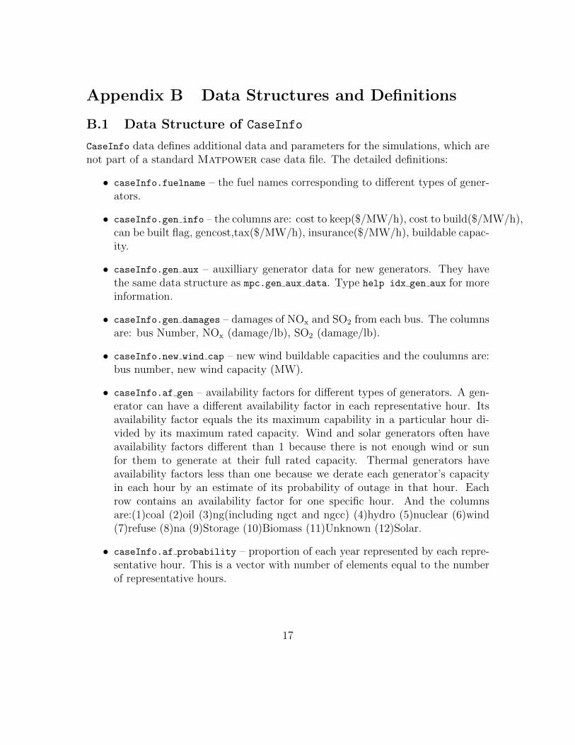
CaseInfo data defines additional data and parameters for the simulations, which arenot part of a standard Matpower case data file. The detailed definitions:

• caseInfo.fuelname – the fuel names corresponding to different types of gener-ators.

• caseInfo.gen info – the columns are: cost to keep($/MW/h), cost to build($/MW/h),can be built flag, gencost,tax($/MW/h), insurance($/MW/h), buildable capac-ity.

• caseInfo.gen aux – auxilliary generator data for new generators. They havethe same data structure as mpc.gen aux data. Type help idx gen aux for moreinformation.

• caseInfo.gen damages – damages of NOx and SO2 from each bus. The columnsare: bus Number, NOx (damage/lb), SO2 (damage/lb).

• caseInfo.new wind cap – new wind buildable capacities and the coulumns are:bus number, new wind capacity (MW).

• caseInfo.af gen – availability factors for different types of generators. A gen-erator can have a different availability factor in each representative hour. Itsavailability factor equals the its maximum capability in a particular hour di-vided by its maximum rated capacity. Wind and solar generators often haveavailability factors different than 1 because there is not enough wind or sunfor them to generate at their full rated capacity. Thermal generators haveavailability factors less than one because we derate each generator’s capacityin each hour by an estimate of its probability of outage in that hour. Eachrow contains an availability factor for one specific hour. And the columnsare:(1)coal (2)oil (3)ng(including ngct and ngcc) (4)hydro (5)nuclear (6)wind(7)refuse (8)na (9)Storage (10)Biomass (11)Unknown (12)Solar.

• caseInfo.af probability – proportion of each year represented by each repre-sentative hour. This is a vector with number of elements equal to the numberof representative hours.

17

• caseInfo.af ex wind – availability factors for existing windfarms. The code iswritten to accommodate a maximum of one wind farm at each bus, and we haveaggregated wind farms in the input data accordingly. Each row is correspondingto one wind farm and each column is corresponding to one representative hour.There are similar definitions for AF of new wind, existing solar and new solar.

• caseInfo.af new wind – availability factors for newly built windfarms.

• caseInfo.af ex solar – availability factors for existing solar.

• caseInfo.af new solar – availability factors for newly built solar.

• caseInfo.af scalemode – “scale mode” means whether availability factors varyby multi-bus area (0) or by individual bus (1) for exWind, exSolar, newWind,newSolar. It’s a 4-element vector.

• caseInfo.af hours – actual representative hours for each contingency

• caseInfo.totalscale – total scale factor for whole network. For example, if theloads we have are from 2013 but we are simulating 2015 and there is expectedto be a 2% load increase from 2013 to 2015 in the region covered by the networkin question, then this scale factor is 1.02.

• caseInfo.loadscale – each row is the load scale factor for each representativehour, since different representative hours have different loads. If there are multiareas each column is the corresponding scale for each area.

• caseInfo.loadgrowth – assumed load growth rate per year. Differs from net-work to network or from area to area.

• caseInfo.dr elasticity – elasticity value.

• caseInfo.dr distcost – assumed average retail cost per MWh on top of thewholesale generation price, in dollars per MWh.

• caseInfo.dr pricevector – vector of multiples of the base-case price at whichload changes.

18

B.2 Data Structure of PolicyInfo

Policy data defines different policies’ input data as follows:

• policy.damage – damage values for CO2 ($/ton), NOx (scaling) and SO2(scaling)emissions.

• policy.damage new – damage values for emissions from newly built generators.

• policy.emission price – include or exclude emission prices in the objectivefunction.

• policy.adj ex genfuel, policy.adj ex – set the fuel price adjustments (permillion Btu) relative to the fuel prices reflected in the basecost column of theMatpower case data file.

• policy.adj new genfuel, policy.adj new – specify the fuel prices of newlybuilt generators.

• policy.wind sub – wind subsidy($).

• policy.elasticity – price elasticity of demand.

• policy.is nuclear – enable or disable the indian point nuclear power plant.

• policy.is newline – enable or disable the new line between New York andQuebec.

• policy.newline data – parameters of the new line.

• policy.year delta – number of years between each stage of simulations.

• policy.retirement – establish whether capacity that was not used in the priortime period will be removed from the generator dataset prior to the beginningof this time period.

• policy.pv costtb – set the hourly cost-to-build per MW of solar.

B.3 Data Structure of E4STResult

19

Table B-1: Data Structure of E4STResult

name description

busID bus number in mpc.bus

genBus bus number in mpc.gen

fuelTypes unique fuel type in mpc.genfuel

genSum generation summed by fuel typegenFuels fuel types for each generatorgenTable installed capacity, used capacity and generation for each generatorbuildableCapSum buildable capacity summed by fuel typeusedCapTabSum used capacity summed by fuel typeInvestCapSum invested capacity summed by fuel typeRetireCapSum retired capacity summed by fuel typeactGenTabSum generation summed by fuel typeloadTable loads at each buslmpTable LMP at each busaverageLoadPrice system average price weighted by loadaverageGenPrice system average price weighted by generationtotalEmissions total emissions for CO2, NOx and SO2 respectivelytotalCO2 total CO2 emissiontotalNOX total NOx emissiontotalSO2 total SO2 emissiondamageCO2 total CO2 emission damagesdamageSONO total NOx and SO2 emission damagestotalTax total tax, which is part of cost to keeptotalInsurance total insurance, which is part of cost to keeptotalFixedcost total fixed costtotalVariablecost total variable costtotalLoad total loadsobjValue objective function valuesgenRawTable complete raw data for each generator

20

References

[1] Daniel L. Shawhan, John T. Taber, Di Shi, Ray D. Zimmerman, Jubo Yan,Charles M. Marquet, Yingying Qi, Biao Mao, Richard E. Schuler, William D.Schulze, and Daniel J. Tylavsky, “Does a Detailed Model of the Electricity GridMatter? Estimating the Impacts of the Regional Greenhouse Gas Initiative,”Resource and Energy Economics, Volume 36, Issue 1, January 2014, pp. 191–207.http://dx.doi.org/10.1016/j.reseneeco.2013.11.015. 1.1, 1.3

[2] Biao Mao, Daniel Shawhan, Ray Zimmerman, Jubo Yan, Yujia Zhu, WilliamSchulze, Richard Schuler, Daniel Tylavsky.“The Engineering, Economic and En-vironmental Electricity Simulation Tool (E4ST): Description and an Illustrationof its Capability and Use as a Planning/Policy Analysis Tool” Proceedings ofthe 49th Annual Hawaii International Conference on System Sciences, Com-puter Society Press, forthcoming January 2016. DOI: (forthcoming) 1.1, 1.3

[3] R. D. Zimmerman, C. E. Murillo-Sanchez, and R. J. Thomas, “Matpower:Steady-State Operations, Planning and Analysis Tools for Power Systems Re-search and Education,” Power Systems, IEEE Transactions on, vol. 26, no. 1,pp. 12–19, Feb. 2011. 1.1

[4] R. D. Zimmerman, C. E. Murillo-Sanchez, and R. J. Thomas, “Matpower’sExtensible Optimal Power Flow Architecture,” Power and Energy Society Gen-eral Meeting, 2009 IEEE, pp. 1–7, July 26–30 2009. 1.1

[5] The BSD 3-Clause License. [Online]. Available: http://opensource.org/

licenses/BSD-3-Clause. 1.2

21